Three-manifolds, Foliations and Circles, I
Preliminary version

Abstract.

A manifold $M$ slithers around a manifold $N$ when the universal cover of $M$ fibers over $N$ so that deck transformations are bundle automorphisms. Three-manifolds that slither around $S^{1}$ are like a hybrid between three-manifolds that fiber over $S^{1}$ and certain kinds of Seifert-fibered three-manifolds. There are examples of non-Haken hyperbolic manifolds that slither around $S^{1}$. It seems conceivable that every hyperbolic 3-manifold slithers around $S^{1}$, and it seems reasonable that every hyperbolic three-manifold has a finite sheeted cover that slithers around $S^{1}$.

If $M$ is a closed $3$-manifold, then I. $M$ slithers around the circle if and only if it has a uniform foliation $\mathcal{F}$, defined to be a foliation without Reeb components such that in the universal cover any two leaves are a uniformly bounded distance apart.

II. Every uniform foliation $\mathcal{F}$ has a transverse flow $\phi_{t}$ that is either pseudo-Anosov, periodic, or reducible (admits a non-empty collection of invariant incompressible tori and Klein bottles).

III. If $M$ is hyperbolic and $\mathcal{F}$ is a uniform foliation of $M$, the stable and unstable laminations for $\phi_{t}$ are quasi-geodesic. The leaves of $\mathcal{F}$ extend continuously to give $\pi_{1}(M)$-equivariant sphere-filling curves in the sphere at infinity of $\tilde{M}$.

IV. The skew ${\mathbb{R}}$-covered Anosov foliations analyzed by Sérgio Fenley [Fen94] slither around the circle. They correspond 1–1 to cocompact extended convergence groups, which are subgroups $\Gamma\subset\widetilde{\operatorname{Homeo}(S^{1})}$ such that $\tilde{T}/\Gamma$ is Hausdorff, where $T$ is the set of counter-clockwise ordered triples of distinct points on the circle. (Convergence groups are the special case that $\Gamma$ contains the kernel ${\mathbb{Z}}\to\widetilde{\operatorname{Homeo}(S^{1})}\to\operatorname{Homeo}(S^{1})$.)

Preview. Two or more further parts are projected in this series. Part II will analyze the asymptotic geometry of leaves of taut foliations of 3-manifolds and construct a universal circle-at-infinity that collates the circles-at-infinity for all the leaves. Provided that $M$ is atoroidal, the action of $\pi_{1}(M)$ on this circle will be used to construct a genuine essential lamination transverse to any taut foliation.

In a subsequent part, we plan to prove the geometric decomposition conjecture for three-manifolds that slither around $S^{1}$ by analyzing the deformation theory of uniform ‘quasi-Fuchsian’ foliations of $M\times{\mathbb{R}}$ whose leaves have three-dimensional hyperbolic structures.

1. Fiberings and Slitherings

Definition 1.1.

One manifold $M$ slithers around a second manifold $N$ when there is a fibration $s:\tilde{M}\to N$ of some regular covering space $p:\tilde{M}\to M$ whose deck transformations are bundle automorphisms for $s$. In other words, deck transformation take each fiber of $s$ to a (possibly different) fiber of $s$. This structure, determined by $s$, is a slithering.

The manifold $M$ is the total space, and $N$ is the base. The fibers of a slithering are the fibers of $s$. The components of the images $p(F)$ in $M$ of the fibers are the leaves of the slithering, and they form a foliation $\mathcal{F}(s)$.

We could always use the universal cover of $M$ for the covering space $\tilde{M}$, but it is sometimes convenient to construct examples in terms of other regular covering spaces. A fibration $M^{m}\to N^{n}$ qualifies as a slithering, but there are many examples that are not of this form. To start,

Example 1.2.

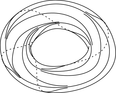
Figure 1. This foliation of $T^{2}$ has two closed leaves; all other leaves are homeomorphic to ${\mathbb{R}}$, spiraling to the two closed leaves at their two ends. Its universal cover can be represented as the foliation of ${\mathbb{R}}^{2}$ by horizontal lines, where the deck transformations are generated (for example) by $(x,y)\longmapsto(x,y+2\pi)$ and $(x,y)\longmapsto(x+1,y+.5\sin(y))$. These transformations act as automorphisms of the fibration ${\mathbb{R}}^{2}\to S^{1}={\mathbb{R}}^{2}/({\mathbb{R}}\oplus 2\pi{\mathbb{Z}})$.

The only closed 2-manifolds that can slither are the torus and Klein bottle, which fiber over $S^{1}$. However, these manifolds also have slitherings that are not fiberings. For instance, figure 1 shows a foliation with two closed leaves, where all other leaves are lines spiraling to the two closed leaves in the two directions. The universal cover of $T^{2}$ can be represented as ${\mathbb{R}}^{2}$ with the foliation by horizontal lines, where deck transformations can be taken as the group generated by

$$\phi(x,y)=(x+1,y+.5\sin(y))\quad\psi(x,y)=(x,y+2\pi).$$

This group acts as automorphisms of the fibering over $S^{1}$

$${\mathbb{R}}^{2}\to{\mathbb{R}}^{2}/({\mathbb{R}}\times 2\pi{\mathbb{Z}})=S^{1}.$$

The particular fibering over $S^{1}$ is part of the data, and is not determined by the foliation (although in many examples, there is a unique simplest choice.) One could, for example, use the fibering over the $2\pi k$ circle ${\mathbb{R}}^{2}/({\mathbb{R}}\times 2\pi k{\mathbb{Z}})$.

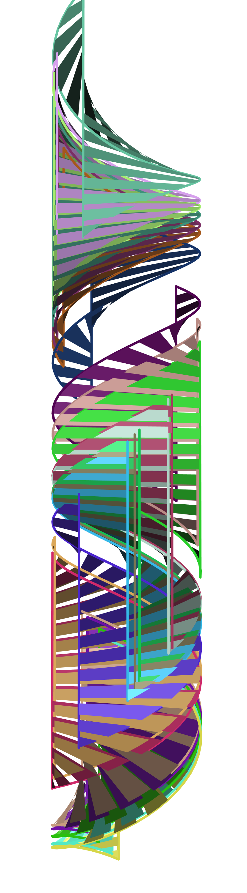
Figure 2. This is the universal cover of the tangent circle bundle of ${\mathbb{H}}^{2}$ (or any hyperbolic surface), with a few randomly selected leaves of its circle-at-infinity foliation. Each leaf is rendered as an assemblage of slats, so we can glimpse what’s behind. This foliation is also called the stable foliation for the geodesic flow. The horizontal direction is the projective disk model for ${\mathbb{H}}^{2}$, while the vertical direction is the angle of a vector in the plane (using ordinary ${\mathbb{E}}^{2}$ measurement.) In these coordinates, one point at infinity on each leaf blows up to a vertical interval. The leaves are portions of helicoids that the foliation has cleverly stacked. Any projective automorphism of the disk has a derivative that when lifted to $\tilde{T}S({\mathbb{H}}^{2})$ preserves this foliation. The unstable foliation for the geodesic flow is obtained by rotating this picture $180^{\circ}$ about its vertical axis.

Example 1.3.

Let $Q^{n}$ be a hyperbolic manifold or orbifold, and let $\operatorname{TS}(Q^{n})$ be its tangent sphere bundle. Then $\operatorname{TS}({\mathbb{H}}^{n})\to\operatorname{TS}(Q^{n})$ is a regular covering, and the map $s:\operatorname{TS}({\mathbb{H}}^{n})\to S_{\infty}^{n-1}$ that sends each tangent ray to its endpoint at infinity is a fibration. The deck transformations act as bundle automorphisms, so $\operatorname{TS}(Q^{n})$ slithers around $S_{\infty}^{n-1}$.

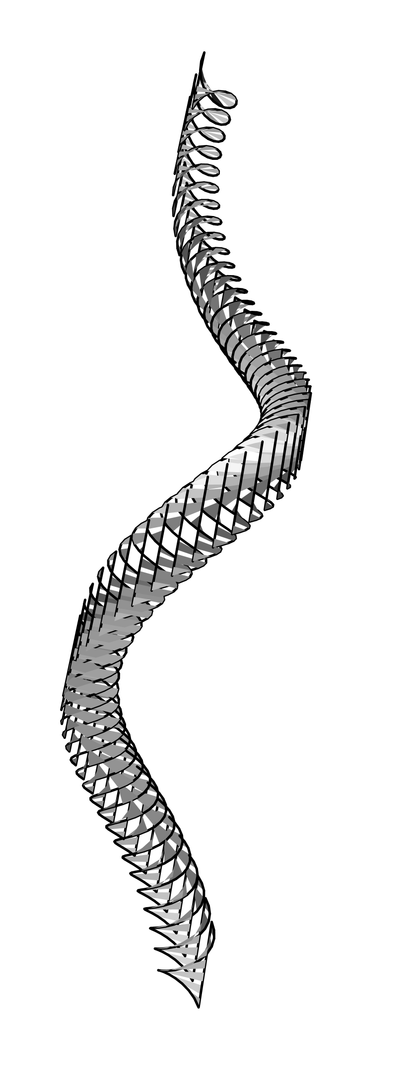
Figure 3. This is the same foliation of $\tilde{\operatorname{TS}}({\mathbb{H}}^{2})$ shown in figure 2, but drawn with every leaf scaled $\times.25$ toward the point where its geodesics are converging, in order to bring out the helical relationship of leaves to points on a circle at infinity.

When $n=2$, the restriction of the bundle $\operatorname{TS}(Q^{2})\to Q^{2}$ to any geodesic in $Q^{2}$ is a torus, and the slithering of $\operatorname{TS}(Q^{2})$ around $S^{1}$ induces a slithering of this torus around $S^{1}$ that is topologically equivalent to the first slithering of the preceding example.

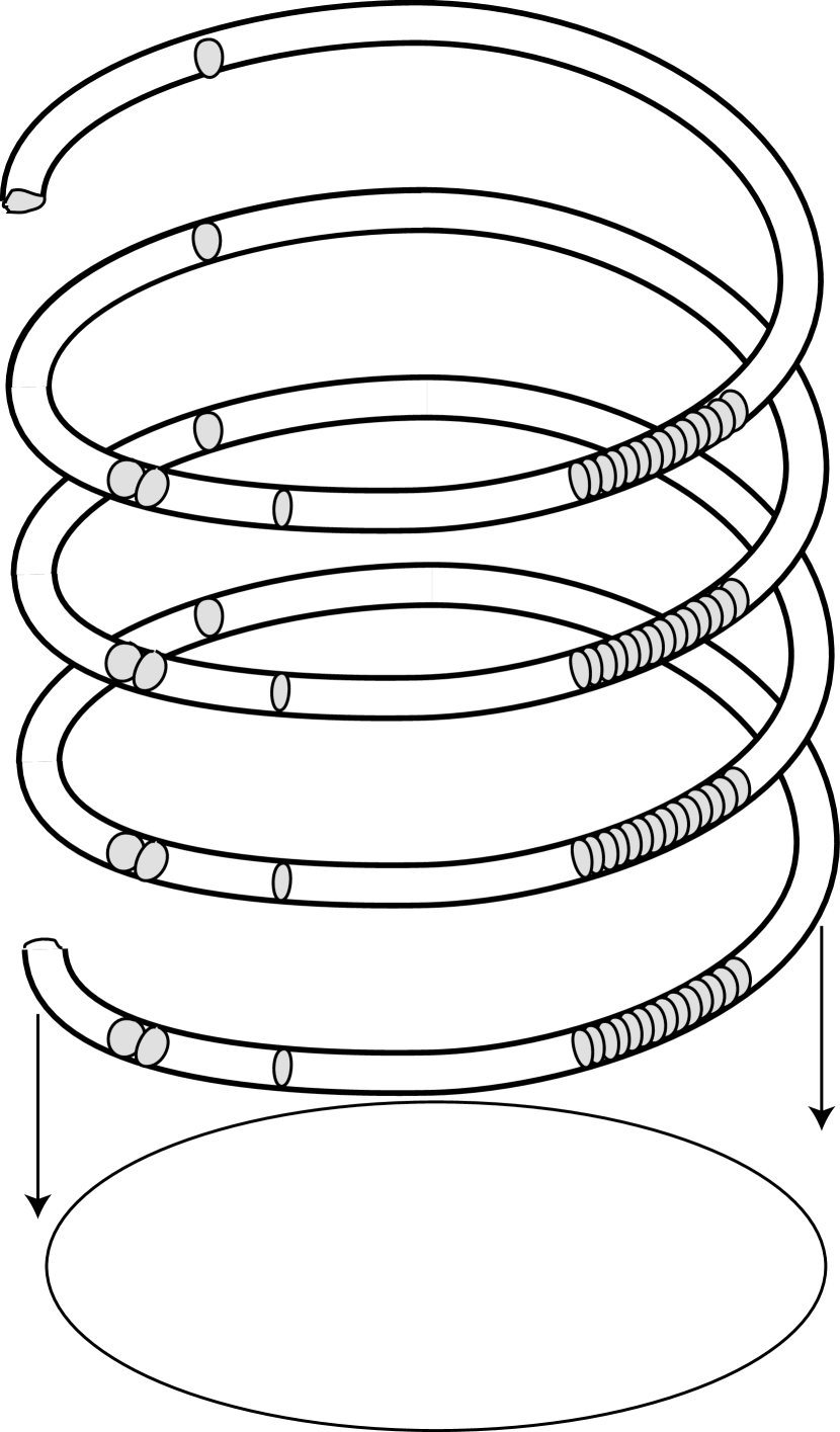
Figure 4. A slithering around $S^{1}$ can be pictured as giving a long, coiled shape to the universal cover $\tilde{M}$. The fundamental domains for the action of deck transformations have projections to $S^{1}$ that are isomorphic, but for a ‘typical’ slithering no two fundamental domains are in phase. The leaves of the foliation of $\tilde{M}$ group into families (a few of them shown) that are the fibers of the slithering. Deck transformations of $\tilde{M}$ move each family as a unit but alter the spacing between fibers. Nonetheless, the distance between any two leaves is bounded by a constant times the number of turns of the coil (2.5.)

When $M^{m}$ slithers around $N^{n}$, then the slithering lifts to a slithering around $\tilde{N}^{n}$. In particular, if the base is $S^{1}$, then the universal cover of $M^{m}$ fibers over ${\mathbb{R}}$. One can picture a long stretched-out image of $\tilde{M}^{m}$, coiled around and around the circle (figure 4.) The fibers of the fibration to $S^{1}$ have infinitely many components. Deck transformations of $\tilde{M}^{m}\to M^{m}$ are periodic, but they probably do not move in a uniform way: in some places the fibers squeeze closer together, while elsewhere they spread apart, reminiscent of the slithering, undulating motion of a snake. A slithering of a manifold around $S^{1}$ has a strong dynamic element, stemming from the hidden action of the fundamental group of $S^{1}$. Slitherings are sneaky structures that you wouldn’t be likely to see if you weren’t on watch for them.

A foliated bundle is a fibration $F^{m-p}\to M^{m}\to P^{p}$ with a reduction to a discrete structure group $\operatorname{Homeo}_{\delta}(F^{m-p})$, that is, a foliation of dimension $p$ transverse to the fibers whose leaves project as covering spaces to $P^{p}$. Any such foliation, when pulled back to the universal cover $\tilde{P}^{p}$ of the base, is a product $\tilde{P}^{p}\times F^{m-p}$. In other words, the leaves define a fibration over $F^{m-p}$, so $M^{m}$ slithers around $F^{m-p}$.

The base can also be an orbifold, and the same reasoning applies. There is a well-developed theory started by Milnor ([Mil58]) and Wood ([Woo69] concerning which circle bundles admit foliations transverse to the fibers when the base is a 2-dimensional orbifold (see section 3.)

Here is another way to represent the data for a slithering, in a compact form that does not mention $\tilde{M}^{m}$. When $M^{m}$ slithers around $N^{n}$, then $\pi_{1}(M^{m})$ acts as a group of homeomorphisms of $N^{n}$. There is a foliated bundle $N^{n}\to E^{n+m}\to M^{m}$ associated with this action, obtained by taking $\tilde{M}^{m}\times N^{n}$ modulo the diagonal action. The graph of the fibration $\tilde{M}^{m}\to N^{n}$ is invariant by the action of $\pi_{1}(M^{m})$, so it descends to give a section $M^{m}\to E^{n+m}$, transverse to the foliation of $E^{n+m}$, and inducing the foliation of $M^{m}$.

For example, assuming $M^{3}$ is compact, a fibration $M^{3}\to S^{1}$ is the same thing as a section of the bundle $M^{3}\times S^{1}\to M^{3}$ that is transverse to the horizontal foliation by $M^{3}\times\theta$ associated with the trivial action. As a second example, when $M^{3}$ is a foliated circle bundle, the fibration can be pulled back to the total space, giving a foliated circle bundle together with a canonical section.

Every slithering gives data of this form, and the data is sufficient to reconstruct the slithering. What’s often not obvious from this type of data is whether or not the map $\tilde{M}^{m}\to N^{n}$ is actually a fibration; this depends on the global structure of $\mathcal{F}(s)$.

For example, a slithering over ${\mathbb{R}}$ gives a codimension one foliation such that the space of leaves of the universal cover is homeomorphic to ${\mathbb{R}}$. However, not every such foliation is a slithering over ${\mathbb{R}}$. For example, consider ${\mathbb{R}}^{3}\setminus\left\{0\right\}$, modulo the action of ${\mathbb{Z}}$ generated by $X\longmapsto 2X$. The quotient is $S^{2}\times S^{1}$. The foliation of ${\mathbb{R}}^{3}$ by horizontal planes restricted to a foliation of the universal cover of $S^{2}\times S^{1}$ such that the space of leaves is ${\mathbb{R}}$; however, this map does not give a fibration over ${\mathbb{R}}$. Furthermore, this foliation can be described as the foliation induced from a section of a foliated circle bundle over $S^{2}\times S^{1}$, the bundle whose fiber is the one-point compactification of the space ${\mathbb{R}}$ of leaves in the universal cover.

Among three-manifolds, the example of $S^{2}\times S^{1}$ is exceptional. Here is a fact from foliation theory:

Proposition 1.4.

Let $\mathcal{F}$ be a codimension one foliation of an irreducible three-manifold $M$. If the space of leaves of the foliation $\tilde{\mathcal{F}}$ in the universal cover $\tilde{M}$ is homeomorphic to ${\mathbb{R}}$, then $\tilde{M}$ is homeomorphic to ${\mathbb{R}}^{3}$, in a way that takes the foliation $\tilde{\mathcal{F}}$ to the foliation of ${\mathbb{R}}^{3}$ by horizontal planes. In other words, $M$ slithers around ${\mathbb{R}}$.

Much more is actually known: Palmeira [Pal78] showed that any foliation of an open $3$-manifold by planes is homeomorphic to the product of ${\mathbb{R}}$ with a foliation of the plane (and similar results in higher dimensions). Poincaré studied foliations (and vector fields) in the plane, and showed that every leaf of a foliation is a properly embedded line. It is easy to deduce that if the space of leaves of a foliation of the plane is homeomorphic to ${\mathbb{R}}$, then the leaves are fibers of a fibration. Haefliger classified all possible foliations of ${\mathbb{R}}^{2}$ in terms of the space of leaves, which is a simply-connected but non-Hausdorff $1$-manifold, together with with certain additional order information at branch points. For present purposes we do not need all this theory.

Proposition 2.9 gives a sufficient condition that can often be used to check whether a section of a foliated circle bundle induces a slithering.

2. Uniform foliations

We will now specialize to the case of main interest: a slithering $s:\tilde{M}^{m}\to S^{1}$ of a compact manifold $M^{m}$ around $S^{1}$. Note that when when $\mathop{\partial}M^{m}\neq\emptyset$, there is an induced slithering of $\mathop{\partial}M^{m}$. The foliation $\mathcal{F}(s)$ is a codimension one foliation transverse to $\mathop{\partial}M^{m}$. In particular if $m=3$ and $M^{3}$ is oriented, its boundary consists of tori.

Any codimension one foliation $\mathcal{F}$ admits a transverse one-dimensional foliation $\tau$ defined by any line field transverse to $\mathcal{F}$. The pair of foliations gives a local ${\mathbb{R}}^{m-1}\times{\mathbb{R}}$ product structure for $M^{m}$. For any parametrized arc $\alpha:[0,t]\to M^{m}$ on a leaf of $\tau$ and any parametrized path $p:[0,u]\to M^{m}$ on a leaf of $\mathcal{F}$, you can ‘comb’ $\alpha$ along $p$ for some distance through the leaves of $\mathcal{F}$. In other words, there is a unique extension $\alpha\times p$ to a maximal monotone subset $H$ of a rectangle, satisfying

$$\alpha\times p:H\subset[0,t]\times[0,u] \to M$$

$$\alpha\times p\,\big{|}\,[0,t]\times 0 =\;\alpha$$

$$\alpha\times p\,\big{|}\,0\times[0,u] =\;p$$

$$\bigl{(}r_{1}\leq r_{2}\;\&\;s_{1}\leq s_{2}\bigr{)} \implies\bigl{(}(r_{2},s_{2})\in H\implies(r_{1},s_{1})\in H\bigr{)}$$

where $\alpha\times p$ maps the two coordinate directions to leaves of the two foliations. In general, $H$ is an open set containing a neighborhood of the two original sides, but not the full rectangle, because the length of $\alpha$ might get longer and longer, whipping out of control and failing to converge in the limit. When the combing is interpreted as partially defining an action of the groupoid of paths along leaves of $\mathcal{F}$ on arcs transverse to $\mathcal{F}$, it is called the holonomy of $\mathcal{F}$.

Definition 2.1.

The foliation $\mathcal{F}$ is regulated by $\tau$ if the holonomy of every arc $\alpha$ exists for all time along any path. It is uniformly regulated by $\tau$ if the lengths of the images of any arc $\alpha$ under the holonomy of $\mathcal{F}$ are bounded, with a bound that depends only on $\alpha$.

A foliation $\mathcal{F}$ is uniform if every closed transverse curve is non-trivial in homotopy, and if for every pair of leaves $L_{1}$ and $L_{2}$ in the universal cover, each is contained in a bounded neighborhood of the other.

Two uniform foliations $\mathcal{F}$ and $\mathcal{G}$ of a manifold $M$ are uniformly equivalent if for every pair of leaves $L$ of $\tilde{\mathcal{F}}$ and $L^{\prime}$ of $\tilde{\mathcal{G}}$, each is contained in a bounded neighborhood of the other.

The prohibition on null-homotopic closed transversals in uniform foliations eliminates examples that have a very different flavor, such as the Reeb foliation (or any foliation) of $S^{3}$. The condition implies that every leaf is properly embedded in the universal cover, since a leaf in the universal cover can never intersect a transverse arc more than once. In dimension $3$, by the celebrated work of Novikov [Nov65], a transversely oriented foliation on any orientable manifold other than $S^{2}\times S^{1}$ satisfies this condition if and only if it does not contain a Reeb component.

It follows from the definition that when $\mathcal{F}$ is regulated by $\tau$, the lifts of $\mathcal{F}$ and $\tau$ to the universal cover of $M^{m}$ define a product structure. Conversely, if the leaves of $\mathcal{F}$ and $\tau$, lifted to the universal cover, are the factors in a product structure, then $\tau$ regulates $\mathcal{F}$. The product structure gives two slitherings for $M^{m}$—a slithering of $M^{m}$ around the universal cover of any leaf of $\mathcal{F}$, and another slithering around ${\mathbb{R}}$ (which is the universal covering of a leaf of $\tau$.) The two foliations complement each other, serving as flat connections for the two slitherings.

When $\mathcal{F}$ is regulated by $\tau$, then it has no null-homotopic closed transversals; if the regulation is uniform, then $\mathcal{F}$ is uniform. If $M^{m}$ is compact and $\mathcal{F}$ is uniform, it easily follows that any $\tau$ that regulates $\mathcal{F}$ regulates it uniformly. This is not true for noncompact $M^{m}$ (e.g. an easy counter-example can be constructed on ${\mathbb{R}}\times S^{1}$.)

In [Ghy87], Étienne Ghys gave an elegant description of a certain equivalence relation on foliated circle bundles in terms of bounded cohomology, and characterized equivalence classes in terms of blowing-up of leaves. This equivalence relation is a special case of uniform equivalence of uniform foliations. Ghys’ characterization of equivalence classes, upon translation to the present context, generalizes to the following:

Proposition 2.2.

Let $\tau$ be a 1-dimensional foliation of a compact $n$-manifold $M$, and let $\mathcal{F}$ and $\mathcal{G}$ be uniformly equivalent uniform foliations of $M$ that are regulated by $\tau$.

If every leaf of $\mathcal{F}$ and of $\mathcal{G}$ is dense, then $\mathcal{F}$ is topologically equivalent to $\mathcal{G}$.

In any case, there is a third uniform foliation $\mathcal{H}$ that can be obtained from each of $\mathcal{F}$ and $\mathcal{G}$ by blowing up at most a countable set of leaves, where each blown-up leaf is replaced by a foliated $I$-bundle.

Proof.

Let $X$ and $Y$ be the spaces of leaves of $\tilde{\mathcal{F}}$ and $\tilde{\mathcal{G}}$; each is homeomorphic to ${\mathbb{R}}$. Let $I\subset X\times Y$ be the closure of the set of pairs of leaves from the two foliations that intersect each other. Each leaf of one foliation intersects an interval’s worth of leaves in the other, since all leaves separate $\tilde{M}$ into two components, so the intersection of $I$ with any line $x\times Y$ or $X\times y$ is a compact interval (possibly a single point.) Therefore, $\mathop{\partial}I$ is the union of two embedded lines (but the lines might intersect each other.) Choose one of the lines, call it $l$. Define a submanifold $M_{l}\subset\tilde{M}\times\tilde{M}$ as a union of copies of $l$, one copy for each leaf of $\tilde{\tau}$—this makes sense because any leaf of $\tilde{\tau}$ is canonically homeomorphic to $X$ and to $Y$.

Observe that $M_{l}$ has the product structure of a leaf of $\tilde{\mathcal{F}}\times l$; it is invariant by the action of $\pi_{1}(M)$, so the quotient $M_{l}/\pi_{1}(M)$ is homeomorphic to $M$, and has a codimension one foliation $\mathcal{H}$. Projection to the two factors shows that $\mathcal{H}$ is a blow-up of $\mathcal{F}$ and $\mathcal{G}$

If leaves of $\mathcal{F}$ and of $\mathcal{G}$ are dense, then the blowing up is trivial, since one of the two projected images of any blown-up region in $\mathcal{H}$ is a proper open invariant subset for one of $\mathcal{F}$ or $\mathcal{G}$. ∎

Given a codimension one foliation, if the induced foliation of its universal cover has a product structure, the foliation is called ${\mathbb{R}}$-covered. The following example shows that not all ${\mathbb{R}}$-covered foliations have uniform spacing of leaves:

Example 2.3.

Let $\phi:T^{2}\to T^{2}$ be an Anosov diffeomorphism of the torus, let $T_{\phi}$ be its mapping torus, let $\mathcal{F}_{s}$ be the stable foliation of $T_{\phi}$, and $\mathcal{F}_{uu}$ be the strong unstable manifold. The universal cover of $T_{\phi}$ is ${\mathbb{R}}\;\times$ the universal cover of $T^{2}$. The foliations $\mathcal{F}_{uu}$ and $\mathcal{F}_{s}$ can be represented in ${\mathbb{R}}^{3}$ by a family of parallel lines and an orthogonal family of parallel planes, so $\mathcal{F}_{uu}$ regulates $\mathcal{F}_{s}$. However, $\mathcal{F}_{s}$ is not a uniform foliation.

However, this example seems to be fairly exceptional. It is hard to construct ${\mathbb{R}}$-covered foliations on ‘generic’ $3$-manifolds. This is partly because it is hard to know the space of leaves in the universal cover, but it seems likely that there is also a fundamental obstruction.

Conjecture 2.4.

A foliation of a closed hyperbolic 3-manifold is ${\mathbb{R}}$-covered if and only if it is a uniform foliation.

Actually, it is remarkable that hyperbolic manifolds can have any kind of ${\mathbb{R}}$-covered foliations at all, since surfaces in hyperbolic space ‘want’ to separate from each other and go off in different directions; most constructions of foliations on hyperbolic manifolds yield foliations which are not ${\mathbb{R}}$-covered. Perhaps it shouldn’t be surprising if ${\mathbb{R}}$-covered foliations on hyperbolic manifolds turn out, as conjectured, to be quite special.

A rough rationale for this conjecture is that when a foliation of a hyperbolic manifold is not uniform, there tends to be recursively nested spreading of the leaves that forces nearby leaves to limit to the sphere at infinity in topologically separated ways. This is related to section 5, which constructs a transverse pseudo-Anosov flow that controls the geometry of leaves of a uniform foliation, and also to section 6, which analyzes how leaves of uniform foliations limit to the sphere at infinity, in continuous, sphere-filling curves. These structures seem likely to occur for any ${\mathbb{R}}$-covered foliation, and they give a fairly explicit conjectural picture of what ${\mathbb{R}}$-covered foliations should look like. See section 7 for a discussion of one class of ${\mathbb{R}}$-covered foliations that do turn out to be uniform.

Proposition 2.5.

If $s$ is a slithering of $M^{m}$ around $S^{1}$, then $\mathcal{F}(s)$ is a uniform foliation.

Proof.

We can define a rough measure of separation between two leaves for a slithering $s$, as follows. Let $\tilde{s}:\tilde{M}^{m}\to{\mathbb{R}}$ be a lift of $s$ to a fibering over ${\mathbb{R}}$, where $S^{1}={\mathbb{R}}/{\mathbb{Z}}$. The fibers of $\tilde{s}$ are connected. Let $L_{r}$ and $L_{t}$ be any two fibers of $\tilde{s}$, that is, leaves in $\tilde{M}$, where $r,t\in{\mathbb{R}}$. The interval $[r,t]$ wraps some whole number of times around $S^{1}$, with some bit left over. Define a function $z(L_{r},L_{t})$ to be the even number $2(t-r)$ when $t-r$ is an integer, and the odd number $2\left\lfloor t-r\right\rfloor+1$ otherwise. With this definition, covering transformation of $\tilde{M}\to M$ preserve the function $z$ on pairs of leaves. Similarly, we define $z(\alpha)$ for any path $\alpha$ in $M$ by taking any lift of $\alpha$ to $\tilde{M}$, and evaluating $z$ on the leaves of its endpoints.

The $z$-diameter of $M$ is the maximum, over all pairs of points $x,y\in M$, of the minimum value of $z(\alpha)$, where $z(\alpha)>0$, $\alpha(0)=x$ and $\alpha(1)=y$. Since $M$ is compact, its $z$-diameter is some finite number $k$. Any arc $\alpha$ in $M$ such that $z(\alpha)>k$ must intersect every leaf of $M$. In fact, if every leaf of $\mathcal{F}(s)$ is dense, then given $x$ and $y$, the leaf through $y$ intersects any transverse arc starting at $x$, so the $z$-diameter of $M$ is $1$.

Let $L$ and $L^{\prime}$ be any two leaves in $\tilde{M}$; assume that $z(L,L^{\prime})>0$. Let $\beta$ be any arc transverse to $\mathcal{F}(s)$ with $z(\beta)=z(L,L^{\prime})+k+2$. We can subdivide $\beta=\beta_{1}*\beta_{2}$, where $z(\beta_{1})>k$ and $z(\beta_{2})>z(L,L^{\prime})$.

For any point $\tilde{x}\in L\subset\tilde{M}$, we can project to $M$, connect the image point $x$ to the $\beta_{1}$ by a path $p$ on its leaf, then lift $p$ and $\beta$ back to an arc $\tilde{\beta}$ in $\tilde{M}$ that intersects $L$ in $\tilde{\beta}_{1}$. Since $z(\beta_{2})>z(L,L^{\prime})$, it follows that $\tilde{\beta}$ intersects both $L$ and $L^{\prime}$. The corresponding lift of $\beta$ intersects $L^{\prime}$, giving an upper bound to the distance from $L$ to $L^{\prime}$.

By symmetry, there is also a bound when $z(L^{\prime},L)<0$—we can, for instance, just reverse the orientation of ${\mathbb{R}}$. ∎

Corollary 2.6.

The distance between any pair of leaves $L$ and $L^{\prime}$ in $\tilde{M}^{m}$ is bounded above by some constant times $|z(L,L^{\prime})|$, and bounded below by some constant times $|z(L,L^{\prime})|-1$.

There is a construction going in the reverse direction, from uniform foliations to slitherings, but it is not an exact converse. We will give a statement expressed in terms of a foliation that is uniformly regulated by a line field. The same proof can be applied to uniform foliations in general, but in this setting the conclusion would be weaker. This is a variation of proposition 2.2, where one is constructing a uniform equivalence from a foliation to itself:

Theorem 2.7.

Let $\mathcal{F}$ be a codimension-one foliation of $M^{m}$ that is uniformly regulated by a 1-dimensional foliation $\tau$.

If every leaf of $\mathcal{F}$ is dense then $M^{m}$ is the foliation of a slithering of $M^{m}$ around $S^{1}$.

In any case, there is a slithering $s:\tilde{M}^{m}\to S^{1}$ of $M^{m}$, regulated by $\tau$ such that $\mathcal{F}(s)$ is uniformly equivalent to $\mathcal{F}$.

Proof.

This could be proven using the same technique as for proposition 2.2, but we’ll express the proof in somewhat different language instead.

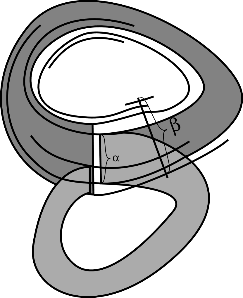
Figure 5. In a uniform foliation, we can start with any transverse arc $\alpha$, and look at all its images under the holonomy of the foliation. The limiting arc $\beta$ cannot expand any wider than it already is. It acts like a pair of calipers that can roughly but consistently measure the transverse distances between leaves, since holonomy images of $\beta$ can never nest with each other.

First we analyze the case that every leaf of $\mathcal{F}$ is dense. Let $\alpha$ be any arc of $\tau$ (see figure 5.) Choose a Riemannian metric on $M^{m}$ (or just a path-metric with reasonable properties, if the data isn’t very smooth). Let $A$ be the supremum of the length of holonomy images of $\alpha$, and let $\beta$ be any arc of length $A$ that is a limit of images of $\alpha$.

Then no holomy image of $\beta$ can have length greater than $A$, since every holonomy image of $\beta$ is a limit of images of $\alpha$. In particular, no holonomy image of $\beta$ can properly contain $\beta$.

Let $l$ be any flow line of $\tau$ in the universal cover, and consider all the lifts of images of $\beta$ to $l$. Since leaves are dense in $M^{n}$, images of both endpoints of $\beta$ are dense. The map that takes each lower endpoint of an image of $\beta$ to its upper endpoint is a well-defined, monotone function from one dense subset of $l$ to another dense subset of $l$, with monotone inverse. Therefore, it extends continuously to a homeomorphism $f:l\to l$. This homeomorphism commutes with the action of $\pi_{1}(M^{n})$.

In other words, the projection of $\tilde{M}^{n}$ to $l$ modulo $f$ is a slithering around $S^{1}$.

If not every leaf of $\mathcal{F}$ is dense, we can still carry out most of the argument. Begin with an arc $\alpha$ of $\tau$ with both endpoints on a minimal set $K$ of $\mathcal{F}$. We obtain a limiting arc $\beta$ that has endpoints on $K$ and whose holonomy images cannot nest with itself. If $l$ is a flow line in the universal cover, then we obtain a monotone function $f$ with a monotone inverse from $K\cap l$ to itself. Therefore $f$ is a homeomorphism of $K\cap l$.

The only possibilities for a proper minimal set such as $K$ in a codimension one foliation is that $K$ is either a closed leaf, or an exceptional minimal set (one where $K\cap l$ is a Cantor set.)

If $K$ is a closed leaf $L$, then $M$ actually fibers over $S^{1}$ with fiber $L$ and structure group $f$; the foliation by fibers of the fibration is uniformly equivalent to $\mathcal{F}$.

If $K$ is an exceptional minimal set, then we can collapse each arc of $\tau\cap M\setminus K$ to obtain a uniform foliation where every leaf is dense, which therefore comes from a slithering. ∎

In high dimensions, one can modify a slithering by taking the connected sum with a simply-connected manifold on each leaf. Sometimes the result is a foliation whose leaves are not homeomorphic: for instance, we could start with a 5-manifold with a slithering similar to example 1.2, with a transverse curve that does not intersect every leaf, then perform the leafwise connected sum with $\operatorname{\mathbb{CP}}^{2}$ along the curve. This indicates the importance of the condition that the foliation of the universal cover is a fibering. It would appear that a variation of this procedure could yield a manifold having a uniform foliation, but no slithering at all.

Example 2.8.

Consider a foliated trivial $I$-bundle over a closed manifold with the top glued to the bottom by a diffeomorphism $\phi$. If there is a homeomorphism $h:I\to I$ that conjugates the holonomy of the bundle to the holonomy composed with $\pi_{1}^{*}(\phi)$, then the resulting foliation is the foliation of a slithering over $S^{1}$, where the structure map $f$ for the slithering is constructed by stringing together copies of $h$. Otherwise, if the holonomy is not invariant at least by some power of $\pi_{1}^{*}(\phi)$, the foliation is not the foliation of a slithering.

This and other similar examples show that foliations constructed by blowing up leaves of $\mathcal{F}(s)$ are not typically foliations of slitherings around $S^{1}$, although they still slither around ${\mathbb{R}}$. The structure map $Z$, which comes from a generator of the group of deck transformation of ${\mathbb{R}}\to S^{1}$, is a leaf-preserving homeomorphism isotopic to the identity in $M$ but usually not isotopic to the identity on a leaf.

Blowing-up operations for slitherings can be naturally performed in terms of the foliated circle bundle over $M$, rather than directly in terms of the foliation.

2.1. Uniform regulation by Lorentz structures

Let $\mathcal{F}$ be a foliation of a compact Riemannian manifold $M^{m}$ that is uniformly regulated by a line field $\tau$. From theorem 2.7 we see that there is some constant $A$ such that given any two leaves $L$ and $L^{\prime}$ in $\tilde{M}$, there is a sequence of intermediate leaves $L=L_{0},L_{1},\dots,L_{n}=L^{\prime}$ such that the distance between $L_{i}$ and $L_{i+1}$ is uniformly bounded by $A$. If $\tau^{\prime}$ is another line field that makes a sufficiently small angle with $\tau$, the flow lines of $\tau$ and $\tau^{\prime}$ stay reasonably close to each other by the time they go a distance of $A$. In particular, we can guarantee that in the universal cover, the flow lines of $\tau^{\prime}$ hit $L_{i+1}$ in a distance only modestly greater than $A$ after they hit $L_{i}$, or in other words, $\mathcal{F}$ is also uniformly regulated by $\tau^{\prime}$.

Estimates for this kind of information can often be conveniently encoded by a Lorentz structure. This can be done with a Lorentz metric, that is, a quadratic form $q$ of signature $(n,1)$, where $\tau$ is contained in the double cone where $q$ is negative. More generally, we could encode the information with an open convex cone in the tangent space of each point (not necessarily a quadratic cone). We’ll call this a Lorentz cone structure. A Lorentz cone structure is transverse to $\mathcal{F}$ if every line contained within the cone is transverse to $\mathcal{F}$. We say that a foliation $\mathcal{F}$ is uniformly regulated by a transverse Lorentz cone structure $C$ if any two leaves $L$ and $L^{\prime}$ in $\tilde{M}$ can be connected by a transverse arc within $C$, and there is a finite upper bound $K(L,L^{\prime})$ for the length of any arc within $C$ connecting $L$ to $L^{\prime}$.

As a limiting case, we will say that a Lorentz cone structure $C$ almost uniformly regulates $\mathcal{F}$ if it is the increasing union of Lorentz cone structures that uniformly regulate $\mathcal{F}$. As an example, consider the foliation by fibers of any actual fibration $M^{n}\to S^{1}$, with the Lorentz cone structure $C$ which is the union of the two open half-spaces that exclude the tangent spaces to the fibers. Then $C$ almost uniformly regulates the foliation. In other examples just as in this one, it is often easiest to describe and think about a limiting case that almost uniformly regulates $\mathcal{F}$.

If $M$ is a manifold with a Lorentz cone structure $C$ and $g:N\to M$ is a differentiable map, we’ll say that $g$ is transverse to $C$ if for each $x\in N$ there is a tangent vector $V\in T_{x}(N)$ taken into $C$, $dg(V)\in C$. In that case, for each open convex half $H$ of the double-cone $C$, the set of vectors that map to $H$ form a convex cone in $T_{x}(N)$, describing a Lorentz cone structure $g^{*}(C)$. We can think of a foliation as a special case of Lorentz cone structure, where each open convex half-cone is a half-space; this definition is a generalization of the definition of a map transverse to a foliation, and of the pullback foliation $g^{*}(\mathcal{F})$.

Proposition 2.9.

If $\mathcal{F}$ is a codimension one foliation of $M$ almost uniformly regulated by a Lorentz cone structure $C$, and if $g:N\to M$ is a differentiable map transverse to $C$, then $g^{*}\mathcal{F}$ is a codimension one foliation almost uniformly regulated by $g^{*}C$.

Proof.

This follows from compactness considerations: if $C^{\prime}\subset g^{*}C$ is a Lorentz cone structure whose half-cones have closure contained in $g^{*}C$, then the images $g(C^{\prime})$ have closure contained in $C$. ∎

It is worth observing that this proposition can be used to give a compact geometric criterion for slitherings in terms of their associated foliated circle bundles. Any foliated circle bundle can be almost uniformly regulated by a Lorentz cone structure $C$, and in particular cases there are explicit constructions using for example curvature estimates. Given a foliated circle bundle $E\to M$, a section $S\to E$ induces a slithering if it is transverse to some $C$.

Figure 6. The tangent to this curve is a time-like curve for the Lorentz structure of $T_{1}(M^{2})$ for certain hyperbolic structures on $M^{2}$. The curve is homotopic to a fiber, since it is the boundary of an immersed disk. An annulus realizing the homotopy in $T_{1}(M^{2})$ intersects itself in short double arcs contained in the regions of self-intersection on the surface. The image of the disk generates $\pi_{1}(M^{2})$, from which one can deduce that the complement of the curve is atoroidal. There are hyperbolic metrics that make the disk round, so in the universal cover view of figure 2 the curve is covered by a countable set of helices, each interlinked with four neighbors. The complement of this curve (or any other time-like curve) slithers around $S^{1}$, as does every cover of $T_{1}(M^{2})$ branched over timelike curves.

Example 2.10.

Let $M^{2}$ be a hyperbolic surface, and $\mathcal{F}$ the circle at infinity foliation of $\operatorname{TS}(M^{2})$ (example 1.3.) The tangent to a horocycle in ${\mathbb{H}}^{2}$ almost traverses the circle at infinity, omitting only one point, where the horocycle is tangent to $S_{\infty}^{1}$. Similarly, a curve in $\operatorname{TS}(M^{2})$ whose base point follows a horocycle in ${\mathbb{H}}^{2}$, lifted to a vector that makes a constant angle to the tangent to the horocycle, but doesn’t point to the point of tangency on $S_{\infty}^{1}$, traverses the entire circle except for that one point. All such curves together sweep out the boundary of a Lorentz cone structure for $\operatorname{TS}(M^{2})$, where a curves in $\operatorname{TS}(M^{2})$ are inside the cone if their vectors turn faster than their base points move. One can think of time-like trajectories as dancers moving in ${\mathbb{H}}^{2}$ in a way that all the scenery, near and far, in front and behind, appears to rotate consistently in one direction. This Lorentz cone structure comes from a Lorentz metric given by the Killing form on $\operatorname{\text{PSL}}(2,{\mathbb{R}})$. This Lie group has the same complexification ($\operatorname{\text{PSL}}(2,{\mathbb{C}})$) as $SO(3)$, and its Lorentz metric lifted to $\operatorname{\text{SL}}(2,{\mathbb{R}})$ has analytic continuation that agrees with the round metric on $S^{3}$.

• If $Q^{2}$ is any closed hyperbolic orbifold and we remove any closed time-like trajectory from $\operatorname{TS}(Q^{2})$, the resulting manifold still slithers around $S^{1}$. There are many possible closed time-like trajectories. For example, the tangent to any curve with curvature greater than 1 is a time-like trajectory; it gives an embedded curve in $\operatorname{TS}(Q^{2})$ as long as it is never tangent to itself.

  Every homotopy class of curves in $Q^{2}$ has infinitely many regular homotopy classes of immersions that can be arranged to satisfy this condition. In fact, all but one of the ${\mathbb{Z}}$’s worth of regular homotopy classes can be made time-like. This can be done by transporting a large-diameter circle immersed in $Q^{2}$ so that its center traverses a geodesic in the base. A pencil speeds around the circle drawing an immersed curve as the circle moves. The pencil travels at constant velocity in parallel-translated coordinates for the circle.

  Furthermore, each time-like regular homotopy class is represented by many distinct time-like knots. In the case of tangents of immersed curves of curvature $>\;1$, the knot type usually changes whenever a tangency between the curve and itself occurs. For the moving circle construction, infinitely many events of this type occur as the circle’s radius tends to infinity.

• If $M^{3}$ slithers around $S^{1}$ and $\mathcal{F}(s)$ is almost uniformly regulated by a Lorentz cone structure $C$, then any branched cover of $M^{3}$ over any time-like link also slithers around $S^{1}$.

• We can remove any time-like curve from $M^{3}$ as above, and replace it by any 3-manifold with torus boundary that fibers over $S^{1}$, to obtain a new manifold that slithers around $S^{1}$.

• Let $\tau\subset M^{3}$ be a $1$-dimensional train-track embedded transversely to $C$. Suppose that we have assigned integral weights to the branches of $\tau$ in a way that satisfies the switch additivity condition. Then we can remove a neighborhood of $\tau$, and for any branch labeled $g$, insert a surface of genus $g$ $\times[0,1]$. We have various choices of gluing maps to glue the ends of the units together at each switch. These can be arranged, if desired, so that the entire inserted assemblage has the same homology as the neighborhood of $\tau$ that was removed. The resulting manifold slithers around $S^{1}$, since it has a map to $M^{3}$ that is transverse to $C$.

In light of the fact that some Seifert fiber spaces are homology spheres, and the fact that there are pseudo-Anosov maps of surfaces that induce every possible symplectic automorphism of first homology, these constructions are powerful enough to produce an atoroidal 3-manifold that slithers around $S^{1}$ with any desired homology type. However, these constructions only scratch the surface, since in these examples the action of $\pi_{1}(M^{3})$ on $S^{1}$ still factors through a Seifert fiber space. The moduli of representations $\pi_{1}(M^{3})\to\widetilde{\operatorname{Homeo}(S^{1})}$ seems to be quite interesting—even when limited to representations in restricted subgroups, such as $\widetilde{\operatorname{\text{PSL}}(2,{\mathbb{R}})}$ or or PL-homeomorphisms—and deserves investigation beyond the present scope.

3. Groups, inequalities and topology

The Milnor-Wood inequality for foliated circle bundles and Stalling’s characterization of fundamental groups of 3-manifolds that fiber over $S^{1}$ demonstrate an interplay of group theory, geometry and topology that is involved in group actions on ${\mathbb{R}}$ and on $S^{1}$, and in manifolds that slither around ${\mathbb{R}}$ or $S^{1}$. This section will recount some of the rudimentary theory of this interaction.

One theme is that groups of periodic homeomorphisms have approximate homomorphisms to ${\mathbb{R}}$, despite the fact that they might not have any actual homomorphisms. This theme can be expressed in several ways.

Proposition 3.1.

Let $a,b,c\in\operatorname{Homeo}_{+}({\mathbb{R}})$ satisfy $[a,c]=[b,c]=1$. Suppose that for all $x\in{\mathbb{R}}$, $c(x)>x$. Then, for all $x\in{\mathbb{R}}$, $c^{-2}(x)<[a,b](x)<c^{2}(x)$.

See figure 7 for a picture of what this is all about.

Figure 7. This diagram shows the commutator of two periodic diffeomorphisms $\alpha$ and $\beta$ of ${\mathbb{R}}$, where $\alpha$ and $\beta$ both have fixed points, but their commutator translates every point downward, sometimes further than one period. By adjusting $\alpha$ and $\beta$, in the limit some points go downward nearly two periods, showing that proposition 3.1 is sharp.

Proof.

For any $x\in{\mathbb{R}}$ there are integers $k$ and $l$ such that

$$c^{k}(x)\leq a(x) <c^{k+1}(x)$$

$$c^{l}(x)\leq b(x) <c^{l+1}(x)$$

Therefore

$$c^{k+l}(x)\leq a(c^{l}(x))\leq a(b(x))<a(c^{l+1}(x))<c^{k+l+2}(x)$$

$$c^{k+l}(x)\leq b(c^{k}(x))\leq b(a(x))<b(c^{k+1}(x))<c^{k+l+2}(x)$$

Let $x^{\prime}=b(a(x))$, so $x=a^{-1}b^{-1}x^{\prime}$. Express the second line of inequalities in terms of $x^{\prime}$, then apply the first, to obtain:

$$c^{-k-l-2}(x^{\prime})<a^{-1}b^{-1}(x^{\prime})\leq c^{-k-l}(x^{\prime})$$

$$c^{-2}(x^{\prime})<aba^{-1}b^{-1}(x^{\prime})<c^{2}(x^{\prime})$$

Since $x^{\prime}$ is arbitrary, this proves the proposition. ∎

Proposition 3.2.

If $G\subset\operatorname{Homeo}({\mathbb{R}})$ acts without fixed points (that is, no element of $G$ except the identity fixes any point in ${\mathbb{R}}$), then $G$ is isomorphic as a group to a subgroup $R(G)$ of the additive group of ${\mathbb{R}}$, with action obtained from $R(G)$ by blowing up at most a countable set of orbits.

(See also 3.5.)

Proof.

If $G$ acts without fixed points, then $G$ has a linear ordering where for $a,b\in G$, $a<b$ if for all $x\in{\mathbb{R}}$, $a(x)<b(x)$. This linear ordering is bi-invariant, that is, if $a<b$ then for all $g\in G$, $ga<gb$ and $ag<bg$.

If there is a least element of $G$ that is greater than $1$, then $G$ is cyclic, and we are done.

Otherwise, given any element $c\in G$ (we imagine $c$ to be small), we can compare the commutator of $a$ and $b$ with powers of $c$; the same inequalities as in proposition 3.1 and its proof hold, but justified now by the bi-invariance of order rather than commutativity. In other words, the commutator of any two elements cannot be greater than the square of any positive element. But there is no lower bound to such squares, because for any $1<c\in G$, if $1<c_{1}<c<c_{1}^{2}$, then $(cc_{1}^{-1})^{2}<(cc_{1}^{-1})(c_{1})=c$. Therefore $[a,b]=1$.

The rest of the statement follows by straightforward reasoning. One method is to construct a measure on ${\mathbb{R}}$ invariant by $G$. The integral of the measure gives a semi-conjugacy of the action to an additive subgroup of ${\mathbb{R}}$—in other words, the action of $G$ is obtained by blowing up at most countably many orbits. ∎

We can apply this information to describe the centralizer of a group of periodic homeomorphisms of ${\mathbb{R}}$. We’ll use coordinates $S^{1}={\mathbb{R}}/{\mathbb{Z}}$, so for all $x\in{\mathbb{R}}$, $g(Z(x))=Z(g(x)$ where $Z(x)=x+1$.

The multiplicative semigroup of ${\mathbb{Z}}$ acts by conjugation on such representations. That is, if $n\neq 0$, we can define a new action $n\times\rho(x)=(1/n)\rho(nx)$. This gives a new action centralized by the supergroup of finite index $(1/n){\mathbb{Z}}$.

Proposition 3.3.

Let $G$ be any group and $\rho:G\to\widetilde{\operatorname{Homeo}_{+}(S^{1})}$ a homomorphism such that all orbits for the action of $\rho(G)$ on ${\mathbb{R}}$ are dense. Then $\rho$ is ${\mathbb{Z}}$-equivariantly conjugate to an action whose centralizer is a closed subgroup of the additive group of ${\mathbb{R}}$. Either $\rho(G)$ is abelian and isomorphic to an additive subgroup of ${\mathbb{R}}$, or $\rho$ is is conjugate to $n\times\rho^{\prime}$ where $n\geq 1$ and the centralizer of $\rho^{\prime}(G)$ is ${\mathbb{Z}}$.

Proof.

Let $Z(\rho(G))\subset\operatorname{Homeo}({\mathbb{R}})$ denote the centralizer of $\rho(G)$. For any element $h\in Z(\rho(G)$, the fixed point set of $h$ is invariant by $G$; since all orbits of $G$ are dense, this implies that either $h$ is the identity, or it has no fixed points. Therefore, $Z(\rho(G))$ is a subgroup of ${\mathbb{R}}$ containing ${\mathbb{Z}}$. If it is cyclic, then $\rho$ is conjugate to a group of the form $n\times\rho^{\prime}$. (We find this conjugacy by looking at the quotient circle ${\mathbb{R}}/Z(\rho(G))$.) Otherwise, $Z(\rho(G))$ is isomorphic to a dense subgroup of ${\mathbb{R}}$. This group cannot have an exceptional minimal set, since $G$ has dense orbits, so the action of $Z(\rho(G))$ on ${\mathbb{R}}$ is standard. ∎

Similarly, if $s:\tilde{M}\to S^{1}$ is a slithering, we can define $n\times s$ by composing with the covering map $S^{1}\to S^{1}$ of degree $n$. We’ll say that a slithering is primitive if it is not isomorphic to $n\times s^{\prime}$ for any $n>1$.

Corollary 3.4.

Let $s:\tilde{M}^{3}\to S^{1}$ be a primitive slithering of a compact $3$-manifold such that every leaf of $\mathcal{F}(s)$ is dense. For simplicity, assume also that $M^{3}$ is orientable and $\mathcal{F}(s)$ transversely orientable. Let $\rho:\pi_{1}(M^{3})\to\widetilde{\operatorname{Homeo}(S^{1})}$ be the action of its fundamental group.

If $\pi_{1}(M)$ contains a non-trivial central element $a$, then either

1. $M^{3}$ fibers over a torus, and $s$ is induced from a slithering of the base, or

2. $s$ admits an invariant measure and is a perturbation of a fibering of $M^{3}$ over $S^{1}$, or

3. the action of $a$ satisfies $\rho(a)(x)=x+l$ for some integer $l$.

Proof.

If $a$ is an element of the center of $\pi_{1}(M^{3})$, then proposition 3.3 says that $a$ acts either as the identity or without fixed points.

If $a$ acts as the identity and if $\mathcal{F}(s)$ has no holonomy, then $\rho(\pi_{1}(M^{3})$ is abelian and admits an invariant measure, by proposition 3.2, so it fits in alternative (ii).

If $a$ acts as the identity and if $b$ is a loop on any leaf $L$ that has non-trivial holonomy, then $a$ and $b$ generate a rank two abelian subgroup of $\pi_{1}(L)$; $L$ is finitely covered by a torus, therefore it is a torus, and $M^{3}$ fibers over $S^{1}$ with fiber $L$. The element $a$ is invariant under the gluing map for this bundle, and so $M^{3}$ can also be described as fibering over $T^{2}$ with $a$ as fiber, where the slithering respects this structure.

If $a$ does not act as the identity, then 3.3 gives us alternatives (ii) or (iii). ∎

3.1. Rotation numbers and commutator length

There are a number of variations and extensions of the inequality 3.1. There is a rich literature on this subject, which started with Milnor’s ([Mil58]) analysis of flat $\operatorname{\text{SL}}(2,{\mathbb{R}})$-bundles. Wood’s paper ([Woo69]) analyzed circle bundles over surfaces by studying $\widetilde{\operatorname{Homeo}_{+}(S^{1})}$ and is close to the present point of view. Other noteworthy references include Eisenbud, Hirsch and Neumann ([EHN81], analyzing Seifert fiber spaces), Sullivan ([Sul76], extending the theory to a more general context and more general bundles) and Ghys ([Ghy87]). We will discuss this topic further in [Thu98] so for now we will make just a quick foray, leaving most details, discussion and development to other sources.

When we have a homomorphism $\rho:G\to\widetilde{\operatorname{Homeo}(S^{1})}$, then for each $a\in G$ there is a rotation number $r(a)\in{\mathbb{R}}$, where $r(a)$ generates the subgroup of ${\mathbb{R}}$ that best approximates the cyclic subgroup generated by $a$. More precisely, $r(a)$ can be characterized as the unique real number such that for all $x\in{\mathbb{R}}$, the difference $|a^{k}(0)-kr(a)|$ has a bound independent of $k$. The value $r(a)\mod{\mathbb{Z}}$ is the same as usual rotation number of the action of $a$ as a homeomorphism of $S^{1}$; the lifting to ${\mathbb{R}}$ is in virtue of the fact that a section is defined for the associated torus bundle over $S^{1}$. One way to define and compute the rotation number is with an invariant measure. There is always at least one measure $\mu$ on ${\mathbb{R}}$ invariant by $a$ such that $[0,1)$ has measure $1$. Then we can define $r(a)=\mu([0,a(0)))=\mu([x,a(x)))$; the characterization of $r(a)$ by boundedness of $|a^{k}(0)-kr(a)|$ is immediate.

An element $a\in G$ is space-like if $a$ has a fixed point, or equivalently, if $r(a)=0$. It is a positive time-like element or simply positive if $r(a)>0$, or equivalently, $\forall x\;a(x)>0$. Negativity is defined similarly.

Using rotation numbers, we can amplify proposition 3.2, for groups of periodic homeomorphisms of ${\mathbb{R}}$:

Proposition 3.5.

Let $G\subset\widetilde{\operatorname{Homeo}_{+}(S^{1})}$ be any subgroup. Then either

1. $G$ is generated by its space-like elements, or

2. the subgroup $G_{0}$ generated by space-like elements has a common fixed point, and consists entirely of space-like elements. This is equivalent to the existence of an invariant measure on ${\mathbb{R}}$ for the action of $G$, and also equivalent to the condition that $r$ (rotation number) is a homomorphism.

Proof.

The graph of a periodic homeomorphism of ${\mathbb{R}}$ can be mapped to the cylinder $\left({\mathbb{R}}\times{\mathbb{R}}\right)/{\mathbb{Z}}$, where ${\mathbb{Z}}$ acts diagonally. The graph becomes a closed curve that represents the generator of the fundamental group of the cylinder. Thus, periodic homeomorphisms are in 1–1 correspondence with closed curves on the cylinder that are transverse to the images of lines parallel to the axes. In rotated coordinates $S^{1}\times{\mathbb{R}}$, they become graphs of functions $S^{1}\to{\mathbb{R}}$ that strictly decrease the metric.

The set $S$ of space-like elements is represented by graphs that intersect the diagonal $\Delta$, which is the graph of the identity. The set $S*S$ of products of two space-like elements is represented by graphs that intersect these; $G_{0}$ is represented by graphs that can be connected to $\Delta$ by a finite sequence of these curves, such that each curve intersects the next in the sequence.

If you can go an unbounded distance in the cylinder by stepping from one curve to intersecting curve, then then the union of the graphs of elements of $G_{0}$ intersects every possible curve in the homotopy class of the generator, so $G=G_{0}$,

Otherwise, let $A$ be the subset of the cylinder consisting of the union of the graphs of elements of $G_{0}$, along with all bounded components of the complement. Note that $A$ is the graph of a symmetric, transitive periodic relation on ${\mathbb{R}}$ (i.e., an equivalence relation) modulo ${\mathbb{Z}}$. From the defining properties, $A$ is invariant by $G_{0}$ and disjoint from its images by non-trivial elements of $G/G_{0}$. These images are linearly ordered. If the linear order is discrete, then $G/G_{0}$ is infinite cyclic. Otherwise, the order-completion is homeomorphic to ${\mathbb{R}}$—this ${\mathbb{R}}$ is the set of equivalence classes of $\tilde{\bar{A}}$. Since $G/G_{0}$ acts on ${\mathbb{R}}$ without fixed points, we can apply 3.2.

For any $x_{0}\in{\mathbb{R}}$, the intersection of line $y=x_{0}$ with $A$ is the minimal interval containing its $G_{0}$-orbit; its upper and lower endpoints are necessarily fixed points for the action of $G_{0}$.

∎

Proposition 3.6.

Let $s_{1},s_{2}:\tilde{M}\to S^{1}$ be two slitherings of a compact manifold $M$ around $S^{1}$. Then $\mathcal{F}(s_{1})$ and $\mathcal{F}(s_{2})$ are uniformly equivalent if and only if the rotation number functions for $s_{1}$ and $s_{2}$ agree up to a constant multiple.

If $\mathcal{F}(s_{1})$ does not admit a transverse invariant measure, then it is uniformly equivalent to $\mathcal{F}(s_{2})$ if and only if $s_{1}$ and $s_{2}$ determine the same sets of space-like elements of $\pi_{1}(M)$.

Proof.

One direction of the proposition is easy: if the foliations are uniformly equivalent, then the rotation number functions agree up to a constant multiple, since the rotation number of $\alpha\in\pi_{1}(M)$ is defined by the asymptotic translation distance of $\alpha^{k}$. The rotation number function up to a constant of course determines the set of space-like elements, which is the set of elements whose rotation number is 0.

In the other direction, suppose that the two rotation number functions $r_{1}$ and $r_{2}$ agree up to a constant multiple, $r_{1}=Cr_{2}$ Consider the map $s_{1}\times s_{2}:\tilde{M}\to{\mathbb{R}}\times{\mathbb{R}}$. We claim that the image of $s_{1}\times s_{2}$ is contained in a bounded neighborhood of a line in the plane. To establish this, choose a compact fundamental domain $K$ for the action of $\pi_{1}(M)$ by deck transformations on $\tilde{M}$. Let $z_{i}$ be the function on pairs of leaves of $\tilde{\mathcal{F}}(s_{i})$ that roughly measures twice the integer part of their separation. Then for any $\alpha\in\pi_{1}(M)$ and any leaf $L_{i}$ of $\tilde{\mathcal{F}}(s_{i})$ we have

$$2r_{i}(\alpha)-1\leq z(L_{i},\alpha(L_{i}))\leq 2r_{i}(\alpha)+1.$$

Applying this to pairs of leaves that intersect $K$, we see that the images $s_{1}\times s_{2}(\alpha(K))$ are at a bounded distance from the line $y=Cx$. By applying corollary 2.6, we see that any such pair of leaves has a uniformly bounded distance, hence all pairs of leaves from the two foliations are contained in bounded neighborhoods of each other.

If $\mathcal{F}(s_{1})$ does not admit a transverse invariant measure, then $\pi_{1}(M)$ is generated by space-like elements. For any $\alpha\in\pi_{1}(M)$, define $g_{i}(\alpha)$ to be the minimum length of its expression as a product of space-like generators, and define

$$h_{i}(\alpha)=\lim_{n}\to\infty\left(g_{i}(alpha^{n})\right)^{1/n}.$$

By considering the cylinder discussed in the proof of proposition 3.5, it is clear that $g_{i}(\alpha)$ can be approximated by a constant multiple of $r_{i}$, up to a bounded additive error term, so $h_{i}$ is a constant times rotation number. Therefore, the set of space-like elements determines the uniform equivalence class of $\mathcal{F}(s_{i})$. ∎

Inequalities such as in proposition 3.1 and its proof can be reworked and extended in terms of rotation numbers. The rotation number of elements of a group $G$ of periodic homeomorphisms can be thought of as a $1$-cochain on the group. Proposition 3.5 describes the circumstances that $r$ is a cocycle, which is equivalent to being a homomorphism. Rotation number is usually not a cocycle, but its coboundary $(\delta r)(a,b)=r(a)-r(ab)+r(b)$ is bounded:

Proposition 3.7.

Milnor–Wood inequality for surfaces with boundary For all $a,b\in G$,

(1) $$\left|(\delta r)(a,b)\right|=\left|r(a)-r(ab)+r(b)\right|\leq 1$$

(2) $$|r([a,b])|\leq 1.$$

Furthermore, if $a_{1},b_{1},a_{2},b_{2},\dots,a_{n},b_{n}$ is any sequence of $2n$ elements of $G$,

(3) $$|r([a_{1},b_{1}][a_{2},b_{2}]\dots[a_{n},b_{n}])|<n+1,$$

In general, for any homomomorphism of the fundamental group of an oriented surface $M^{2}$ with boundary into $\widetilde{\operatorname{Homeo}_{+}(S^{1})}$, the sum of the rotation numbers of its boundary curves does not exceed $\max(0,-\chi(M^{2}))$.

Proof.

The various inequalities all follow from the statement about an oriented surface with boundary: (1) is the case of pair of pants, (2) is a punctured torus, and (3) is a punctured surface of genus $n$.

Here is a sketch of a proof. Given the representation of $\pi_{1}(M^{2})$, let $\xi\to M^{2}$ be the associated foliated circle bundle, with section $S:M^{2}\to\xi$ that is defined up to homotopy by the structure group $\widetilde{\operatorname{Homeo}_{+}(S^{1})}$. Choose a complete hyperbolic metric of finite area on $M^{2}$, and lift this to give a hyperbolic metric for the leaves of the foliation. By [Gar83], there is a harmonic measure for this foliation, which can be normalized so it gives measure $2\pi$ to each fiber, which assigns an $\operatorname{\text{SO}}(2)$ structure to each fiber, and makes the bundle into a principle $\operatorname{\text{SO}}(2)$-bundle. The foliation gives a plane field transverse to the fibers; average the slopes of the images of this plane field under the action of the circle $\operatorname{\text{SO}}(2)$. The resulting connection has curvature that never exceeds $1$. Near the cusps, it converges to a flat connection whose slope is $2\pi$ times the rotation number for the corresponding boundary component.

This implies that the integral of the curvature does not exceed $-2\pi\chi(M^{2})$, which translates into the inequality that the sum of rotation numbers of the boundary components is not greater than the Euler characteristic of $M^{2}$. ∎

Remark 3.8.

There are better inequalities in the cases when the the rotation numbers are not all integers. For instance, if $0<r(a)<1$, then for all $x$, $a^{-1}(x)>x$, and the same holds for the conjugate: $ba^{-1}b(x)<x$. It follows that

$$r([a,b])=r(a*(ba^{-1}b^{-1}))<r(a),$$

and similarly $r([a,b])>r(a^{-1})$. If $1-r(a)<r(a)$, we can get a better inequality by using the fact that $aba^{-1}b^{-1}=(aZ^{-1})b(Za^{-1})b^{-1}$ and applying the same reasoning. Continuing along the same path, as long as at least one of $r(a)$ or $r(b)$ is not an integer, we can approximate it by the nearest power of $Z$, and deduce that $r([a,b])\leq 1/2$. It is curious that when $r(a)$ and $r(b)$ are both $0$ (or other integers), then $r([a,b])$ can attain $\pm 1$, as shown by the the tangent bundle of a once-punctured surface, or by the example of figure 7.

This is related to the fact that most periodic homeomorphisms with a rational rotation number have neighborhoods in the group of homeomorphisms where the rotation number is constant. In particular, the cases of integral rotation numbers are big baskets. In $\widetilde{\operatorname{\text{PSL}}(2,{\mathbb{R}})}$, these baskets contain one lift for every hyperbolic element.

For an element $g$ of the commutator subgroup $G^{\prime}=[G,G]$, the commutator length $\operatorname{cl}(g)$ is the minimum number of commutators $[a_{i},b_{i}]$ whose product equals $g$. This is a sub-additive function: $\operatorname{cl}(gh)\leq\operatorname{cl}(g)+\operatorname{cl}(h)$. When $g$ is not in $G^{\prime}$, then we can define $\operatorname{cl}(g)=\infty$. Define $\operatorname{acl}(g)=\liminf_{n\to\infty}1/n\operatorname{cl}(g^{n})$; we’ll call this the asymptotic commutator length of $g$; it is finite if and only if $\alpha$ maps to an element of finite order in $H_{1}(M)$

Corollary 3.9.

If $M$ slithers around $S^{1}$, then for any $\alpha\in\pi_{1}(M)$,

$$r(\alpha)\leq\operatorname{acl}(\alpha).$$

A 3-manifold whose fundamental group contains a central element $\alpha$ cannot slither around $S^{1}$ unless $M$ is a nilmanifold or $\operatorname{acl}(\alpha)\geq 1$.

A 3-manifold whose fundamental group contains a normal ${\mathbb{Z}}^{2}$ subgroup cannot slither around $S^{1}$ unless $M$ has a Euclidean or nilgeometry structure.

This contains a version of the Milnor-Wood inequality expressed in terms of slitherings: for a circle bundle of Euler class $n$ over $M^{2}$, the fiber has order $n$ in homology. The asymptotic commutator length of the fiber is $\chi(M^{2})/n$, which must be at least $1$ to admit a foliation transverse to the fibers.

Proof.

The inequality on rotation numbers follows from equation 3. The application to 3-manifolds whose fundamental group has a center follows from 3.4.

Rotation number is a linear function on any abelian subgroup of $\pi_{1}(M)$: this follows directly from the definition, and also is a consequence of inequality 1 of proposition 3.7. If there is a normal $Z^{2}$ subgroup $A\subset\pi_{1}(M^{3})$, then the linear function $\rho\,\big{|}\,A$ must be invariant by conjugacy, if $\mathcal{F}(s)$ is transversely orientable, otherwise it is invariant up to sign. If $M^{3}$ is orientable, this implies there is a common eigenvector with eigenvalue identically $1$ for the conjugacy action of $\pi_{1}(M^{3})$ on $A$, i.e., there is a central ${\mathbb{Z}}\subset\pi_{1}(M^{3})$.

In the non orientable or non-transversely-orientable cases, there still is a normal ${\mathbb{Z}}$ whose centralizer necessarily has index at most two. It still follows that $M^{3}$ fibers with fiber a circle with Euclidean base, but besides the torus, the base might be a Klein bottle ($(\mathsf{XX})$ in Conway’s orbifold notation), or any of the Euclidean 2-orbifolds whose non-trivial local groups have order $2$: an annulus ($**$), a Moebius band ($*\mathsf{X}$), a pillow ($2222$), a sack ($22*$) or a cross-sack ($22\mathsf{X}$). ∎

4. Geodesic currents

The uniformization theorem says that every Riemannian metric on a surface is conformally equivalent to a metric of constant curvature. Alberto Candel ([Can93]) analyzed how the uniformization varies from leaf to leaf in a lamination with 2-dimensional leaves. In particular, he showed that if $\mathcal{F}$ is a codimension one foliation of an irreducible 3-manifold that either the foliation is a perturbation of a foliation with torus leaves, or there is a Riemannian metric that has constant negative curvature on each leaf. This Riemannian metric varies continuously, but may not be very differentiable in the manifold as a whole. We will not concern ourselves here with questions of regularity of the metric, since we will really only use the quasi-isometric properties, which are not delicate at all. If preferred, the metric of constant curvature $-1$ on each leaf can be approximated by a $C^{\infty}$ or even $C^{\omega}$ Riemannian metric on $M$ that induces a metric on each leaf whose curvature is pinched between $-1-\epsilon$ and $-1+\epsilon$; such a metric would be more than adequate for what we will do.

Given any Riemannian metric for the leaves of a codimension one foliation $\mathcal{F}$ of a closed $3$-manifold $M^{3}$, let $T_{1}(\mathcal{F})$ denote the unit tangent bundle of the leaves of $\mathcal{F}$, and let $\operatorname{Gfl}:{\mathbb{R}}\times T_{1}(\mathcal{F})\to T_{1}(\mathcal{F})$ denote the geodesic flow on the leaves.

Every flow on a compact space admits at least one invariant measure; usually, there are many different invariant measures. Here is a more explicit method to find invariant measures, in the case of $\operatorname{Gfl}$ for the foliation $\mathcal{F}(s)$ of a slithering $s$ of a compact $3$-manifold $M$. Proposition 3.5 says that the normal closure of the fundamental groups of the leaves of $\mathcal{F}(s)$ is the kernel of a homomorphism (typically the trivial homomorphism) of $\pi_{1}(M)$ to a subgroup of ${\mathbb{R}}$. The image group consists of periods (integrals around closed curves) for a transverse invariant measure equipped with a transverse orientation, turning it into a closed current (which is a generalization of a closed $1$-form.) If $\pi_{1}(M)$ is not abelian, the kernel is automatically non-trivial, therefore there are non-simply-connected leaves. The only case of an $M$ that slithers around $S^{1}$ (or more generally, has a codimension one foliation) such that all leaves are simply-connected is when $M=T^{3}$. Note that in this case, the leaves of the foliation are not hyperbolic.

For any non simply-connected leaf, there must be a closed geodesic on the leaf—this follows from the fact that the leaves have complete Riemannian metrics with injectivity radius bounded from below. In a negatively curved metric, any curve that is nearly geodesic is near a geodesic, so it is easy to find a closed geodesic in each homotopy class, by curve-shortening. Even in metrics for the leaves where there are no stipulations on the curvature, we could apply a curve-shortening process to get curves on leaves that are more and more nearly geodesic; such a curve might not converge on its own leaf, but we could take a limit in $M^{3}$ to get a closed geodesic on some leaf. This gives an invariant measure.

For a non-singular flow such as $\operatorname{Gfl}$, we can factor any invariant measure as a transverse invariant measure $\times\;dt$, where $dt$ denotes the measure of time along flow-lines and coincides with arc length of a geodesic, in the case of the geodesic flow; a transverse invariant measure is a measure locally defined on the local space of orbits that is invariant under holomy. The advantage of converting to a transverse invariant measure is that it is a better topological invariant—intuitively, a transverse invariant measure is something very similar to a closed orbit; it can be thought of like a limit of ${\mathbb{R}}$-linear combinations of $1$-manifolds, and is a special case of a closed $1$-current, which is a version of a ${\mathbb{R}}$-1-cycle. That is, a transverse invariant measure gives a linear function on $1$-forms on $T_{1}(\mathcal{F})$, obtained by an iterated integral, first integrating the $1$-form over flow-lines, then integrating with respect to a transverse invariant measure. Transverse invariance of the measure is equivalent to the condition that this linear function vanishes on $df$, for any function $f$.

Given a foliation with a Riemannian metric for its leaves, let $\operatorname{MG}(\mathcal{F})$ denote the space of transverse invariant measures for the geodesic flow. If the manifold is compact, this is the cone on a compact convex set (using the weak topology on transverse invariant measures).

Suppose now that we have a $3$-manifold $M^{3}$ that slithers around $S^{1}$, with a Riemannian metric that is negatively curved on the leaves. Let $Z:\tilde{M}\to\tilde{M}$ be a homeomorphism that is a lift of a generating deck transformation of ${\mathbb{R}}\to S^{1}$. For any leaf $L$ of $\tilde{\mathcal{F}}(s)$, $Z(L)$ is a bounded distance from $L$. Furthermore, every leaf is sandwiched between two iterates $Z^{k}(L)$ and $Z^{k+1}(L)$.

Lemma 4.1.

For each pair of leaves $L$ and $L^{\prime}$ in $\tilde{M}$ and every infinite geodesic $g$ on $L$, there is a unique geodesic $g^{\prime}$ on $L^{\prime}$ at a a bounded distance from $g$.

Proof.

Although the leaves are not quasi-isometrically embedded in $\tilde{M}$, they are properly embedded, since any fiber intersects any transverse curve at most once. In fact, the leaves are uniformly properly embedded, in the sense that for any constant $A$ there is a constant $B$ such that any two points on $L$ who have distance less than $A$ in $\tilde{M}$ have distance less than $B$ along $L$. To see this fact, consider any sequence of shortest geodesic arcs along leaves in $\tilde{M}$ whose endpoints have distance in $\tilde{M}$ not exceeding $A$. Adjusting by covering transformations and passing to a subsequence, we may assume that the two endpoints converge. Since the space of leaves in $\tilde{M}$ is Hausdorff, the pair of endpoints is on a single leaf. The limit points are at a bounded distance on their leaves, therefore, the length of the approximating arcs are bounded, and their lengths converge to the distance between the limit points.

Let $C$ be the maximum separation between $L$ and $L^{\prime}$ (so every point on either leaf has a point within distance $C$ on the other). Given any geodesic $g$ on $L$, we can choose a sequence of points $\left\{p_{i}\right\}$ on $g$ at uniform intervals, say $1$, and find points $q_{i}$ within distance $C$ of $p_{i}$ on $L^{\prime}$, giving a path on $L^{\prime}$ whose length is increased at most by some constant factor. We can also go from geodesics on $L^{\prime}$ to paths on $L$ that increase at most by a constant factor. This means that quasi-geodesics on either leaf correspond to quasi-geodesics on the other. In ${\mathbb{H}}^{2}$, or any other complete metric of pinched negative curvature on ${\mathbb{R}}^{2}$, every quasi-geodesic is a bounded distance from a unique geodesic. This establishes the lemma. ∎

Corollary 4.2.

If $s$ is a slithering of a 3-manifold $M^{3}$ around $S^{1}$ with hyperbolic leaves, then there is a canonical identification of the circles at infinity for all the leaves of $\tilde{\mathcal{F}}(s)$, giving a single $\pi_{1}(M)$-equivariant circle. In other words, the circles at infinity for the leaves of $\mathcal{F}(s)$ forms a foliated circle bundle over $M$.

Proof.

A geodesic on a leaf $L$ of $\tilde{M}$ is determined by a pair of distinct points on its circle at infinity. The bounded-distance correspondence between geodesics on $L$ and geodesics on another leaf $L^{\prime}$ has to preserve this product structure, since two geodesics converge to the same point at infinity if and only if their distance in that direction stays bounded. ∎

Note that this circle bundle is not in general isomorphic to the associated circle bundle of the slithering: for example, in the case of a 3-manifold that fibers over $S^{1}$ with fibers of negative Euler characteristic, the slithering bundle is trivial, and the tangent circle bundle of the fibers is not. However, section 7 discusses a situation when these two bundles coincide.

5. Canonical transverse flows

A 3-manifold $M$ that has a slithering $s$ around $S^{1}$ has a foliation $\mathcal{F}(s)$, but it also has a somewhat mysterious extra piece of dynamics, the map $Z$ defined on the space of leaves of the foliation in $\tilde{M}$ which comes from the deck transformations of the universal cover of the circle. In this section, we will analyze the action of $Z$ on geodesic currents on the leaves, enabling us to enhance $Z$ by constructing a connection for the slithering, canonical up to conjugacy by a homeomorphism isotopic to the identity. In other words, we will find a 1-dimensional foliation transverse to $\mathcal{F}(s)$ and uniformly regulating it. Assuming transverse orientability, if we isotope $M$ along flow lines until each point goes once around the circle, the result is a leaf-preserving homeomorphism of $M$ that lifts to induce the automorphism $Z$ of the space of leaves of the universal cover.

First, we can enhance $Z$ to define a map from $T_{1}(\mathcal{F})$ to itself that gives an automorphism of the foliation by geodesics (flow-lines of $\operatorname{Gfl}$), using a standard trick. In the unit tangent space of the foliation of $\tilde{M}$, first construct a $\pi_{1}(M)$-equivariant continuous map $f_{1}$ that takes each point on a geodesic on a leaf $L$ to some point at distance at most $A$ on the corresponding geodesic on $Z(L)$. This is readily constructed by making local choices and using a partition of unity to average them. Now, define $f(x)$ to be the average of $f_{1}(\operatorname{Gfl}_{t}(x))$ where $t$ ranges over a long interval $[-T,T]$. Since each flow-line has an affine structure, averaging makes sense. It is easy to verify that $f_{1}$ is quasi-monotone, that is, it eventually progresses in a single direction. The quasi-monotonicity of $f_{1}$ implies monotonicity of $f$. (An alternative way to do this is to use triples of points on the circle at infinity for the leaves.)

The automorphism $Z$ of $T_{1}(\mathcal{F})$ induces an automorphism of the space of transverse invariant measures, which we also denote $Z:\operatorname{MG}(\mathcal{F})\to\operatorname{MG}(\mathcal{(}F)$. If we denote $\operatorname{PG}(\mathcal{F})$ the set of non-zero transverse invariant measures up to scaling, then $Z$ acts as a projective endomorphism on $\operatorname{PG}(\mathcal{F})$.

Every projective endomorphism of a compact convex set has at least one fixed point, by Perron-Frobenius theory. In other words, it follows from general principles that there is some transverse invariant measure $\mu$ for $\operatorname{Gfl}$ that is taken to a multiple of itself by $Z$. We’ll describe below a method to find such a $\mu$. (A projective endomorphism of a compact convex set is a generalization of a positive matrix, and a fixed point for the transformation is a generalization of a positive eigenvector).

Here’s one fairly explicit way to obtain such a measure $\nu$. Let $\mu$ be any invariant measure for $\operatorname{Gfl}$. The mass $|\mu|$ of a transverse invariant measure $\mu$ is the mass of $\mu$ converted back to an actual measure $\mu\times ds$. We consider all the images $Z^{k}(\mu)$ for $k>0$, and look at the maximal growth rate (or decay) of its mass,

$$g(\mu)=\limsup_{k\to\infty}\left(\frac{|Z^{k}(\mu)|}{|\mu|}\right)^{1/k}.$$

We will define a sequence of weighted averages of $Z^{l}(\mu)$ that is more and more nearly a $1/g(\mu)$ eigenmeasure for $Z$. We can do this by choosing weights for the first $2N$ iterates such that for the first $N$ terms the weight of each term is slightly more than $1/g(\mu)$ times the weight of the preceding, for the last $N$ terms, slightly less than $1/g(\mu)$ times the preceding. We can choose weights of this sort so that most of the total comes from the middle $N$ terms of the sequence, provided $N$ is a number so that for $l>N$ the estimates for $g(\mu)$ are not very much too high, and for some of the middle terms they are near the limit. The weighted sum, normalized to have mass $1$, is nearly a $1/g(\mu)$-eigenmeasure. Any limit point of this sequence gives an eigenmeasure.

There is a kind of linking number between invariant measures for $\operatorname{Gfl}$ that will help give us a better geometric understanding of the action of $Z$. This notion is a generalization of the intersection number of two measured geodesic laminations or geodesic currents on a surface. In the case of a compact surface $S$, the geometric intersection number $i(\mu,\nu)$ is a symmetric bilinear function of transverse invariant measures. This geometric intersection number is the integral of the product measure $\mu\times\nu$ over all intersection points of geodesics on $S$. If the injectivity radius of $S$ is $\geq a$, then we can associate to any intersection point of two geodesics $g,h$ the subset of $T_{1}(S)\times T_{1}(S)$ consisting of the pair of segments of radius $a$ on $g$ and $h$; different intersections map to disjoint sets. Therefore, $a^{2}i(\mu,\nu)<|\mu||\nu|$. The length of a geodesic is a special case of the intersection number with the natural Riemannian volume element for the geodesic flow, that is, the intersection number with a ‘random’ geodesic. This fits into a picture for Teichm”uller space analogous to the Lorentz space model of ${\mathbb{H}}^{n}$, see [Thu85].

To generalize intersection numbers to the geodesic flow $\operatorname{Gfl}$ for $\mathcal{F}$, we will say that two geodesics on leaves in $\tilde{M}$ cross if their projections to any single leaf intersect. (See figure 8.) We want to think about crossings modulo the action of $\pi_{1}(M)$. The way to record this information (a pair of geodesics modulo deck transformations) is with a homotopy class of paths $\alpha$ between flow-lines of $\operatorname{Gfl}$, where each endpoint of $\alpha$ can slide along but not leave its flow line. A path of this sort determines a crossing if for a lift to the universal cover, the geodesic of its first endpoint crosses the geodesic of its second.

For any crossing $\alpha$, we can give a measure of the height difference of its endpoints, by setting $z(\alpha)=2k$ if $Z^{k}$ takes $\alpha(0)$, lifted to the universal cover, to the leaf of $\alpha(1)$, and $z(\alpha)=2k+1$ if, lifted to $\tilde{M}$, the leaf of $\alpha(1)$ is between the leaf of $Z^{k}(\alpha(0))$ and $Z^{k+1}(\alpha(0))$. This definition makes $z$ anti-symmetric in $\alpha$, that is, $z(\alpha)=-z(\alpha^{-1})$ where $\alpha^{-1}$ is the same path in the reverse direction. Since the bounds for quasi-isometric comparisons between geodesics on different leaves depend only on the value of $z$, every crossing is represented by a path $\alpha$ whose length is bounded as a function only of $z(\alpha)$.

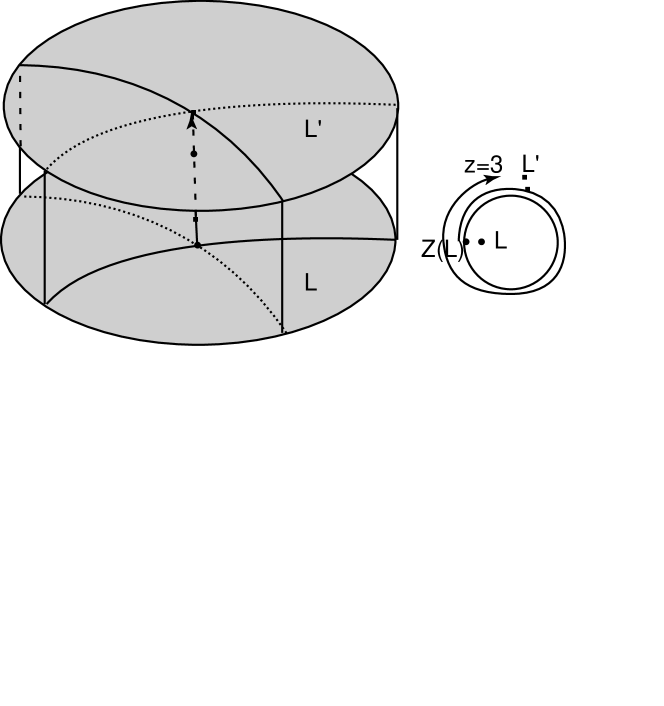
Figure 8. This is a sketch of two leaves in the universal cover of a slithering, with two geodesics. The circles at infinity of the leaves are identified, so we can tell whether or not the geodesics cross. Crossings modulo deck transformations are identified by the homotopy class of a path that joins them. Given two geodesics currents $\mu$ and $\nu$ (measures on geodesics on the leaves), we aggregate all the crossings into the linking series $\Lambda(\mu,\nu)$ according to the $z$-value of a path that joins them.

Given two geodesics on leaves of $\tilde{M}$, we can quantify crossing data by grouping pairs of geodesics according to the value of $z$. We encode this information in a formal Laurent series, integrating over all crossings $\alpha$:

(4) $$\Lambda(\mu,\nu)=\int_{\alpha}t^{z(\alpha)}\mu\times\nu$$

Convergence of the integral can be checked similarly to convergence in the definition of intersection number of laminations on surfaces. If the injectivity radius of $M$ is $a$, then given an arc $\alpha$, any other arc joining points on segments of radius $a$ on the geodesics of its endpoints and staying within $a$ of $\alpha$ represents the same crossing. The space of arcs of length less than $B$ is compact; each coefficient is dominated by an integral of a locally bounded measure over a compact space, therefore is bounded. This reasoning shows that for each $k$ there is some constant $C_{k}$ such that the coefficient of $t^{k}$ in $\Lambda(\mu,\nu)$ is not greater than $C_{k}\left|\mu\right|\left|\nu\right|$.

The constant term of $\Lambda(\mu,\nu)$ measures the actual intersections.

$$\Lambda(\mu,\nu)(t)=\Lambda(\mu,\nu(1/t).$$

The coefficient of $t$ measures how much $\mu$ intersects $\nu$ when each geodesic is swept through $M$ to its image under $Z$. Other coefficients are similar. This linking series is not continuous as a function of $\mu$ and $\nu$: when even terms are non-zero, it’s sometimes possible for $\mu$ and $\nu$ to have arbitrarily small perturbations where some or all of the weights on even terms jump to neighboring odd terms.

If $\mu$ and $\nu$ are invariant measures, note that

$$\Lambda(\mu,\nu)=t^{2}\Lambda(Z(\mu),\nu)=t^{-2}\Lambda(\mu,Z(\nu)).$$

This implies that the coefficients of $\Lambda(\mu,\nu)$ grows at most exponentially fast. In other words, the portion with positive exponent converges in some neighborhood of $t=0$, and the portion with negative exponent converges in a neighborhood of $t=\infty$. Of more immediate significance is the consequence that the linking series is invariant when both arguments are transformed by $Z$. This implies that if $\mu$ is any eigenmeasure for $Z$ with eigenvalue not 1, then $\Lambda(\mu,\mu)$ is identically $0$. It also implies that if $\mu$ and $\nu$ are any two eigenmeasures for $Z$ such that $\Lambda(\mu,\nu)\neq 0$, then their eigenvalues are reciprocal.

Proposition 5.1.

Either

• The action of $Z$ on geodesic currents is globally bounded, that is, there is some constant $K$ such that for every transverse invariant measure $\mu$ for $\operatorname{Gfl}$ and for every integer $k$,

  $$\left|Z^{k}(\mu)\right|<K\left|\mu\right|,$$

  or

• there is a transverse invariant measure $\nu$ for $\operatorname{Gfl}$ that is an eigenmeasure of $Z$ and such that $\Lambda(\nu,\nu)=0$

Proof.

Suppose that the action of $Z$ on geodesic currents is not globally bounded, so there is a sequence $\left\{\mu_{i}\right\}$ of transverse invariant measures for $\operatorname{Gfl}$ of mass $1$, and integers $\left\{k_{i}\right\}$ such that $\left\{\left|Z^{k_{i}}(\mu_{i})\right|\right\}$ tends to $\infty$. Then the sequence of normalized transforms $\left\{\mu^{\prime}_{i}=Z^{k_{i}}(\mu_{i})/\left|Z^{k_{i}}(\mu_{i})\right|\right\}$ has the property that all the coefficients of $\Lambda(\mu^{\prime}_{i},\mu^{\prime}_{i})$ tend to $0$ as $i$ tends to $\infty$, in light of equation 5. We can pass to the limit, and obtain an invariant measure $\mu$ for $\operatorname{Gfl}$. Even though $\Lambda$ is not in general continuous, it follows in this case that $\Lambda(\mu,\mu)=0$, since the terms of the limit only have contributions from the limits of neighboring terms. In other words, there are no crossings at all between geodesics in the support of $\mu$, in no matter what homotopy class $\alpha$. The set $\sigma$ consisting of all geodesics on leaves of $\mathcal{F}$ that do not cross geodesics in the support of $\mu$ forms a closed set, invariant under $\operatorname{Gfl}$ and under $Z$. Therefore, there is a transverse invariant measure $\nu$ for $\sigma$ that is projectively invariant by $Z$. ∎

Remark 5.2.

It can happen that the masses of images of invariant measures are unbounded, yet the only positive eigenmeasures for $Z$ have eigenvalue $1$. This happens, for example, with the mapping torus of a Dehn twist $T_{\gamma}$ around a non-trivial curve $\gamma$ on a negatively curved surface. In this case, $Z$ acts on fibers as $T_{\gamma}$; it represents isotoping of the mapping torus once around the circle. For any curve $\beta$ that crosses $\gamma$, the images $Z^{k}(\beta)$ grow to infinity in length, while the normalized transverse invariant measure supported on $Z^{k}\beta$ converges to $\gamma$, which is an eigenmeasure of eigenvalue $1$.

A slithering $s$ of $M^{3}$ is reducible when there is an embedded incompressible torus or Klein bottle where $s$ induces a slithering. A torus of this form is a reducing torus (or Klein bottle if it’s a Klein bottle.) It is known from foliation theory that in a foliation of a 3-manifold without Reeb components, any incompressible torus is isotopic to a transverse torus, or a leaf in the special case of a foliation whose leaves are all tori. Consideration of the various cases shows that a torus transverse to $\mathcal{F}(s)$ is a reducing torus, unless $M$ fibers over $S^{1}$ or $I$ with fiber a torus (which does not imply that $s$ is itself a fibration.)

Before proceeding further with the generic case B of proposition 5.1, the non-generic case A has an interesting story:

Theorem 5.3.

(Convergence group theorem, Gabai [Gab92] and Casson and Jungreis, [CJ94]) In case A of proposition 5.1, $M$ is a Seifert fiber space and the slithering is a foliated circle bundle.

Proof.

Note: this is not a new proof, but simply a reduction of the current statement to a standard established form.

The analysis of this case is a consequence of a long, winding series of developments starting with Nielsen, who settled the case mapping torus case, which is equivalent to—Nielsen showed that if some power a diffeomorphism $\phi$ of a surface is homotopic to the identity, then $\phi$ is isotopic to a diffeomorphism of finite order, which implies that the mapping torus of $\phi$ can also be described as a Seifert fiber space. We will not attempt to recount the history, nor to fit the present application naturally into context. However, it’s worth remarking that the hypothesis (A) is close to the condition that $\pi_{1}(M)$ acts as a group of uniform quasi-isometries of the hyperbolic plane, which is close to the condition that it acts on the circle as a convergence group, meaning its action on triples of points on the circle is properly discontinuous. It’s also worth remarking that the set of triples of points on a circle, modulo a convergence group, comes naturally equipped with a slithering around $S^{1}$.

We will content ourselves here with deriving the theorem logically from established knowledge. For this, it will be sufficient to find an immersed incompressible torus. Assuming $M$ is not $T^{3}$ (where the theorem is more trivially true), not all the leaves of $\mathcal{F}(s)$ are simply connected. Let $\gamma$ be a non-trivial curve on any leaf. Choose a base-point $*\in M$, and for each image $Z(\gamma)$ connect $\gamma$ by a shortest path to $*$. This gives a sequence of homotopy classes of bounded length, so they repeat infinitely often. We can form a long immersed cylinder connecting all the images $Z^{k}(\gamma)$ and intersecting each leaf in a geodesic, not necessarily closed, but converging to the same end points on $S_{\infty}^{1}$. The homotopy information tells us that this this cylinder eventually joins up, forming a torus or Klein bottle.

If $\mathcal{F}(s)$ is reducible, then it decomposes into geometric pieces by the geometrization theorem for Haken manifolds. Hyperbolic pieces are incompatible with immersed incompressible non-boundary-parallel tori. Taut foliations of Seifert fiber spaces have been understood for some time—the Haken cases were analyzed in [Thu72], and the non-Haken cases followed from later developments. In general, a taut foliation of a Seifert fiber is isotopic to be transverse to the fibers provided the fiber is not homotopic to a leaf. If the base is a negatively-curved orbifold, the only possibility for $\mathcal{F}(s)$ to be isotopic so that it is transverse to the fibers. It can happen that the leaves of $s$ are ‘vertical’ when the base is Euclidean, but then (given condition A) there is some other Seifert fibration transverse to the leaves.

If $s$ arises by sewing together Seifert fiber pieces along tori in a way that fibers cannot be chosen to align, then a geodesic current that crosses an offending torus violates hypothesis A (just as in remark 5.2.)

If $M$ is torus-irreducible but has an immersed incompressible torus, the culmination of the long development mentioned above implies that $M$ must be a Seifert-fiber space. ∎

We need to think about the topology as well as the measure theory of the action of $\pi_{1}(M)$ on $\operatorname{Gfl}$. To develop the topological picture a little further, consider any $L$ in $\tilde{M}$. The fundamental group of $M$ acts on the set of geodesics in $L$. Consider any closed invariant subset $I$ for this action. Form an $\epsilon$-neighborhood $I_{\epsilon}$ (on $L$) of the union of geodesics in $I$. We claim that if $I_{\epsilon}$, or any connected component of $I_{\epsilon}$, does not limit to all of $S_{\infty}^{1}$, then $s$ is reducible. To see this, let $X\subset S_{\infty}^{1}$ be any proper subset that is the limit set for some component of $I_{\epsilon}$, and form the convex hull $H$ of $X$ in the hyperbolic metric on $L$. Each element of $\pi_{1}(M)$ takes $H$ to itself or to a set that is disjoint except possibly on one boundary line. More specifically, it is possible to have two distinct boundary lines in a single $\epsilon$ disk on $L$, but not three. Now consider all the images of boundary lines of $H$ back in $M$, transported to all leaves of $\mathcal{F}(s)$. The union is compact, since $M$ is compact and each sheet of the surface swept out by the boundary lines has a uniform neighborhood intersecting at most one other sheet. Therefore, the union is a compact surface. The surface has an induced slithering, which means its Euler characteristic is $0$, so it is a torus or Klein bottle.

Note in particular that if there is some $\epsilon$ such that $I_{\epsilon}$ is not connected, then any component of $I_{\epsilon}$ has a limit set $X$ that is a proper subset of $S_{\infty}^{1}$, so $s$ is reducible.

We will say that a $\pi_{1}(M)$-invariant set $I$ of geodesics fills $M^{3}$ if for every $\epsilon$, $I_{\epsilon}$ is connected, and its limit set is the entire circle at infinity. As we have seen, if $s$ is irreducible, then every $I$ fills $M$.

If there are crossings in $M$ among the geodesics in $I$, then there may not be a clear choice of a canonical form for the immersed surfaces swept out by $I$ in $M$—this is the usual problem, that whenever three or more lines cross each other, there are multiple patterns in which they can cross, and it is hard to choose among them. However, when there are no crossings, $I$ sweeps out a topologically well-defined 2-dimensional lamination $S(I)$ in $M$, intersecting each leaf in the geodesic lamination covered by $I$.

Lemma 5.4.

If $I$ is a closed $\pi_{1}(M)$-invariant subset of geodesics with no crossings, then the gaps of $I$ are dense, that is, no neighborhood in ${\mathbb{H}}^{2}$ is foliated by geodesics in $I$.

Proof.

If any open set is swept out by geodesics, one or the other endpoint of the geodesics actually moves. If we go toward a non-constant endpoint in ${\mathbb{H}}^{2}$, the geometric limit is a foliation of ${\mathbb{H}}^{2}$ by geodesics having one endpoint constant and the other endpoint completely traversing the remainder of the circle. Since $M$ is compact, this behavior would actually occur in the intersection of $S(I)$ with some leaf, and hence in every leaf. It follows that $\pi_{1}(M)$ would have a fixed point on $S_{\infty}^{1}$, so the action of $\pi_{1}(M)$ on a leaf is solvable. There is enough information in this picture to determine that $M$ would have to be commensurable with the mapping torus of an Anosov diffeomorphism of the $T^{2}$, as developed in the analysis of Dehn surgeries on the figure eight knot in Thurston, [Thu79]. However, the foliations compatible with this foliation are not of the form $\mathcal{F}(s)$. ∎

It is easy to see that $S(I)$ is an essential lamination. Each gap in the lamination $I$ sweeps out a submanifold of $M$, which is a gap in $S(I)$ . If we truncate the 3-dimensional gaps where the geodesic sides approach within $\epsilon$, we obtain a finite number of compact 3-manifold with walls that alternate being geodesics on their leaves and $\epsilon$-hops from one geodesic wall to another. If $s$ is irreducible, then the gaps are solid tori, in the form of ideal polygons that wrap around through $M$ and return with some rotation.

Proposition 5.5.

If $s$ is an irreducible slithering that has an invariant set $I$ of non-crossing geodesics, then $s$ is regulated by a flow $\phi_{t}$ that preserves the 2-dimensional lamination $S(I)$.

Proof.

We can first construct the flow $\phi$ on $S(I)$ by first making a rough but bounded guess, then averaging along the geodesics. If the flow is chosen continuously on $S(I)$, we can easily extend continuously to the solid torus gaps. ∎

Proposition 5.6.

Let $s$ be an irreducible slithering of a closed three-manifold $M^{3}$ around $S^{1}$ which is not in case A of 5.1 (i.e., is not a Seifert fiber space, by 5.3). Let $\lambda$ be the largest sustained growth factor for any lamination under positive or negative iterates of $Z$, that is,

$$\lambda=\limsup_{|k|\to\infty}\left(\frac{|Z^{k}(\mu)|}{|\mu|}\right)^{1/k}$$

Then there are two transverse invariant measures $\mu_{s}$ and $\mu_{u}$ for $\operatorname{Gfl}$ that are $\lambda$ and $1/\lambda$ eigenmeasures for $Z$.

Proof.

We can use the procedure described above to find an eigenmeasure whose transverse invariant measure shrinks in a direction that the growth factor is attained. Say this is $\mu_{u}$, whose transverse invariant measure grows for negative $k$.

Now let $\nu$ be any measure such that $\Lambda(\mu_{s},\nu)\neq 0$, from a construction of section 4. Because $\mu_{s}$ is a $\lambda^{-1}$ eigenmeasure of $Z$, this series has the form $(a_{0}+a_{1}t)\sum_{k}\lambda^{-k}t^{2k}$. In other words, $\nu$ crosses $\mu_{s}$ more and more for negative time, with the measure of crossings growing by a factor of $\lambda$ at each stage. This can only happen if the mass of $\nu$ grows geometrically, comparable to $\lambda^{-k}$ for $k<0$. We can construct a $\lambda$-eigenmeasure by taking any limit point $\mu_{s}$ of weighted combinations of these images under $Z^{-k}$. ∎

So far, we have not logically deduced the geometric relationship between $\mu_{u}$ and $\mu_{s}$. It is logically consistent with proposition 5.6 and its proof (even if this may seem bizarre geometrically) that $\mu_{u}$ and $\mu_{s}$ are mutually singular measures that are physically supported on the same invariant subset of $\operatorname{Gfl}$. Our next task is to analyze this geometry, so that, in particular, we will be able to use eigenmeasures for $Z$ to construct a pseudo-Anosov flow transverse to $\mathcal{F}(s)$.

We suppose that $s$ is an irreducible slithering of a closed 3-manifold $M$ with transversely oriented foliation $\mathcal{F}(s)$, and that $\nu$ is a transverse invariant measure for $\operatorname{Gfl}$ and eigenmeasure for $Z$ with eigenvalue $\lambda<1$. Let $I_{\nu}\subset L$ be the support of $\nu$. Define $M_{L+}$ to be closed halfspace of $\tilde{M}$, on the positive side of $L$, and $M_{L-}$ similarly. If we project geodesics in $M_{L+}$ to $L$, this induces a map on transverse invariant measures; since $\lambda<1$, the contributions of $\nu$ to the projection decrease exponentially as a function of the height function $z$, so this gives a well-defined transverse invariant measure for $I_{\nu}$. Let’s call this image $L_{+}(\nu)$. (We could also have projected just the contribution from a fundamental domain $0\leq z<2$, which would give a transverse invariant measure for $I_{\nu}$ no matter what the value of $\lambda$.)

Note that the corresponding measure on $Z(L)$ is the measure on $L$ multiplied by $\lambda$:

$$Z^{k}(L)_{+}(\nu)=\lambda^{k}L_{+}(\nu).$$

Lemma 5.7.

$L_{+}(\nu)$ has no atoms, that is, there is no single geodesic of $I_{\nu}$ with positive transverse measure.

Proof.

If there were any atoms for $L_{+}(\nu)$, its images under negative powers of $Z$ would have arbitrarily large mass; this is incompatible with compactness of $M$ and the finite mass of $\nu$. ∎

Let’s focus on one gap $G$ on $L$, and look at what happens along one of its sides $g$ (where $g$ is a geodesic). Choose a short arc $J$ transverse to $I_{\nu}$ and connecting $G$ to another gap. Then $J\cap I_{\nu}$ is a Cantor set, since gaps are dense and there are no atoms to $L_{+}(\nu)$. Define $\mathcal{G}\subset{\mathbb{R}}$ to be the collection of values of the $\nu$-measures along $J$ from $G$ to other gaps; then $\mathcal{G}$ is a dense subset of the interval $[0,\nu_{J}]$.

There are infinitely many gaps in $I_{\nu}$, but each of them is an ideal polygon that is a lift of the intersection of one of the finitely many solid tori gaps in $S(I_{\nu})$. This implies that there is bounded variability of the geometry and of the transverse invariant measure among all the gaps of $I_{\nu}$ wherever they appear, among all the leaves of $\tilde{M}$.

Let $S(G)$ be the solid torus gap in $M$ swept out by $G$. We can follow the solid torus once around, giving a return map of $G$ to itself. The return map $R_{G}$ of $G$ might take $g$ to a different side of $G$, but some iterate $R_{g}=R_{G}^{p}$ takes $g$ back to itself. The return map is not in general a power of $Z$, and will not in general take $L_{+}(\nu)$ projectively to itself, but nonetheless the return map is sandwiched between two powers of $Z$: if $\alpha$ is an arc in the homotopy class of $R_{g}$, which can be identified with a deck transformation of $\tilde{M}\to M$ that does the right thing to $g$, then it is sandwiched between $\left\lfloor z(\alpha)/2\right\rfloor$ and $\left\lceil z(\alpha)/2\right\rceil$ power of $Z$, translating to the inequalities

$$\lambda^{\left\lceil z(\alpha)\right\rceil}L_{+}(\nu)\leq R_{g}^{*}L_{+}(\nu)\leq\lambda^{\left\lfloor z(\alpha)\right\rfloor}L_{+}(\nu).$$

Since the transverse measure for $I_{\nu}$ shrinks when pushed forward by the return map, this says that the leaves of $I_{\nu}$ have to spread further from each other. We are aiming to construct particular return maps that balance the separation of geodesics by quasi-uniformly shortening them.

We may assume that $J$ is short enough so that it cuts each gap it intersects other than $G$ into a single tip of the ideal polygon on one side, and the thick part of the ideal polygon on the other. $R_{g}$ sends $J$ to some arc $R_{g}(J)$ transverse to $I_{\nu}$; no matter how $J$ was chosen, at least some initial segment of this image arc crosses the same leaves as an initial segment of $J$. We may replace $J$ by a segment that has an $I_{\nu}$-preserving isotopy to an initial segment of $R_{g}(J)$.

Now construct an annulus $S(J)$ transverse to $S(I_{\nu})$ by sweeping $J$ around $S(G)$, always intersecting the same set of leaves until it returns via $R_{g}$; at that point, glue an initial segment to $J$. The figure formed is like a one-tooth saw-blade slicing through layers of $S(I_{\nu})$ (figure 9.)

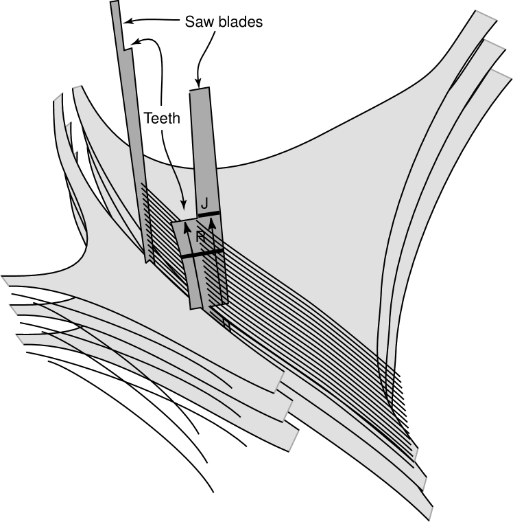
Figure 9. Saws cutting through laminations

We can continue in the same vein, to construct a family $S(J_{i})$ of disjoint saw-blade annuli, one for each annular face of each solid torus gap of $S(I_{\nu})$. Only the tooth of a saw-blade cuts through $S(I_{\nu})$; except for the tooth, the rim is in a gap.

Every leaf of $S(I_{\nu})$ is dense in $S(I_{\nu})$—otherwise, its closure would either contain all of $S(I_{\nu})$ except for isolated leaves, which we have ruled out by lemma 5.7, or it would be small enough to give us a reducing torus. It follows that the saw blades $S(J_{i})$ have sliced each geodesic of $I_{\nu}$ on each leaf of $\mathcal{F}(s)$ into bounded intervals.

We can group these intervals of geodesics according to their homotopy class rel saw blades. On any one leaf of $\mathcal{F}(s)$, they group into a locally finite collection of parallel bundles. Topologically, if the parallel arcs in one bundle are squeezed together to one arc, the collection of arcs plus intersections of saw-blades divides the surface into compact simply-connected regions, which become polygons if the saw-blade intersections are collapsed to points. The polygons come from gaps of $I_{\nu}$ and from ends of the saw-blade intersections (or both).

In three dimensions, a set of parallel arcs sweeps out sheets (like a layer pastry). In the downward direction, sheets can run into saw teeth, where they are cut into two pieces. If there were any family of arcs that could be isotoped downward forever, then the arcs would have to stay bounded in length forever. The arc defines a homotopy class of paths between the cores of the two solid tori; there are only finitely many homotopy classes of bounded length, so eventually this homotopy class repeats, joining to form an annulus that gives a homotopy of some power of the core of one solid torus to some power of the core of some solid torus (possibly the same). The intersection of the annulus with leaves of $\mathcal{F}(s)$ gives homotopy classes of arcs between two gaps; however, because $\lambda\neq 1$, these arcs would have zero intersection number with $L_{+}(\nu)$, which is impossible. Therefore, every sheet of arcs is split by a saw-tooth in the downward direction. In the upward direction, every sheet that is not an original gap boundary eventually runs off the edge of a saw tooth, where it merges with other sheets. In the three-dimensional picture in $M$, only finitely many homotopy classes of arcs occur, where each homotopy class $\beta$ serves as an index pointing to a family $P_{\beta}$ of parallel rectangular sheets. Let $t_{\beta}\in[0,1]$ be a parameter for the vertical direction of $P_{\beta}$, so that $t_{\beta}$ locally parameterizes the leaves of $\mathcal{F}(s)$ within a rectangular solid that encloses $P_{\beta}$.

At this stage, we can apply the automorphism $Z$, that is, turn on the saws, after first adjusting the blades into proper alignment. For each solid torus gap, attach the hubs of all its saw blades to the core circle. The image of a saw-blade under $Z^{-1}$ intersects fewer leaves; it is isotopic to a subset of itself. If we modify $Z$ using such an isotopy, then the image of the each saw blade under $Z$ contains the saw blade. We can also arrange the flow $\phi$ to be tangent to the saw blades and to their edges, so that $Z$ takes each saw blade to the same flow line. Under iteration of $Z$, the blades expand indefinitely, by consideration of the measure $L_{+}(\nu)$. Their edges remain bounded in length, since they traverse a bounded $z$-length. As the saw blades expand, they remain transverse to the intervals of $I_{\nu}$, chopping them successively into more and more pieces. In other words, the blades appear to converge to a lamination that has a finite number of leaves with a singularity at the core of each solid torus gap of $S(I_{\nu})$. To make a precise definition of a limiting lamination, we can consider the order type of intersections of the saw blades with the arcs $\beta$. The union of all intersections gives a countable linearly-ordered set on each homotopy class of arcs. The order completion of any countable linearly-ordered set (completion with Dedekind cuts, adjoining an upper and lower endpoint if needed) is a compact linearly-ordered set $X_{\beta}$ that has an order-preserving embedding in the unit interval unique up to homeomorphism (and might well be an interval.) For each $\beta$, form the product of $X_{\beta}$ with a rectangle; we’ll assemble these pieces to form a singular foliation transverse to $\mathcal{F}(s)$ and to $S(I_{\nu})$. For each $\beta$, we have a rectangular solid, with a foliation or lamination already in two coordinate directions. The new leaves have automatic gluing maps at their top and bottom faces, since these come from the cutting edges of the saw blades, where each intersection continues through. The horizontal faces work similarly.

For the sake of symmetry, we can blow up the resulting lamination along its singular leaf, replacing the singular leaf with a solid torus gap, having new leaves in the form of annuli for each ‘side’ of the singular leaf. We’ll call this new lamination $S^{*}(I_{\nu})$. The intersections of leaves of $S^{*}(I_{\nu})$ with leaves of $\mathcal{F}(s)$ form a 1-dimensional foliation $I_{\nu}^{*}$, that is, $S^{*}(I_{\nu})=S(I_{\nu}^{*})$. Each leaf of $I_{\nu}^{*}$, lifted to $\tilde{M}$, converges to distinct points at its two endpoints, on account of its transversality to the geodesic lamination $I_{\nu}$. (The leaves of $I_{\nu}$ describe neighborhood bases for all points at infinity except the vertices of its gaps; the leaves of $I_{\nu}^{*}$ do not stay in any gap of $I_{\nu}$, and cross $I_{\nu}$ at angles bounded from below.) Therefore, each leaf of $I_{\nu}^{*}$ is homotopic to a unique geodesic. The homotopies can be made uniformly bounded, using the compactness of $M$. We straighten out all the leaves of $I_{\nu}^{*}$ to geodesics; it doesn’t matter if conceivably this collapses multiple leaves to a single leaf, since the process is invariant from leaf to leaf. The resulting lamination is still transverse to $I_{\nu}$, so we can simply make this adjustment, keeping the same names $I_{\nu}^{*}$ and $S^{*}(I_{\nu})$ for the 1-dimensional and 2-dimensional laminations.

Now we apply previous constructions, to obtain an invariant measure $\nu^{*}$ on $I^{*}_{\nu}$ which is a $1/\lambda$ eigenmeasure for $Z$. We obtain a measure $L_{-}(I_{\nu}^{*})$ on each leaf. By examining the possible gaps, which necessarily are ideal polygons, it’s clear that its support must be all of $I^{*}_{\nu}$.

To summarize and slightly extend:

Theorem 5.8.

Let $s:\tilde{M}\to S^{1}$ be a slithering of a compact $3$-manifold $M$. Then $M$ splits along some (possibly empty) family of reducing tori into a finite number of pieces. On each of the pieces, the induced slithering is either a foliation transverse to the fibers of a Seifert fiber space, or it admits a transverse pseudo-Anosov flow $\phi_{t}$ (or possibly a pseudo-Anosov line field, if $\mathcal{F}(s)$ is not transversely orientable) whose stable and unstable foliations are uniquely determined by $s$.

Proof.

In the case of a closed manifold with an irreducible slithering, we are nearly done. We have already addressed the case that lengths of invariant measures for the geodesic flow transform boundedly.

We should recall here that if the leaves of $\mathcal{F}(s)$ do not have hyperbolic type, then $\mathcal{F}(s)$ admits a transverse invariant measure (for instance, by Candel, [Can93]), and $s$ is a perturbation of a mapping torus of a diffeomorphism of $T^{2}$ (or possibly a bundle over $S^{1}$ with fiber a Klein bottle, or a bundle over the $I$ orbifold, if we do not make assumptions of orientability and transverse orientability). In this situation, the theorem is easily verified.

If lengths of invariant measures transform unboundedly but have eigenvalue $1$, we still get an eigenmeasure $\nu$ for $Z$ whose support has no crossings (proposition 5.1.) The eigenvalue $1$ implies there is a transverse invariant measure for $S(I_{\nu})$. Such a measure is expressible as a cohomology class with coefficients twisted by the transverse orientation of $S(I_{\nu})$. It can be perturbed to a rational class, which gives a perturbed 2-dimensional lamination having nearby support, all of whose leaves are closed. These leaves have foliations induced from $\mathcal{F}(s)$, so they are toruses, and $s$ is reducible.

If there is an eigenmeasure $\nu$ for $Z$ of eigenvalue $\neq 1$, we have the two laminations $S(I_{\nu})$ and $S^{*}(I_{\nu})$ constructed in the preceding discussion. By a familiar technique (see e.g. [Thu79]), given $\mathcal{F}(s)$, $S(I_{\nu})$ and $S^{*}(I_{\nu})$, we obtain a decomposition of $M$ consisting of intersections of leaves and/or gaps from the three. If we collapse the elements of this decomposition, we obtain a homeomorphic manifold where the laminations are singular foliations, intersecting in $1$-dimensional foliation. Every arc of the flow of $z=1$ multiplies $L_{+}(\nu)$ by $\lambda$ and $L_{-}(\nu*)$ by $1/\lambda$. We can adjust the transverse metric so that the transverse flow steadily compress in one normal direction while expanding in the other, making it a pseudo-Anosov flow. Given uniqueness of the pseudo-Anosov foliations, the non-transversely-orientable case can be obtained from the transversely oriented double cover.

Any other invariant measure $\mu$ for the geodesic flow has to have crossings either with $\nu$ or with $\nu^{*}$, so its eigenvalue is determined, and it can have no crossings with the other of the two. This implies uniqueness of the geodesic laminations $I_{\nu}$ and $I_{\nu}^{*}$, which implies uniqueness of the pseudo-Anosov foliations.

When $s$ has torus boundary, for each boundary component, we can take a horoball in ${\mathbb{H}}^{3}$ modulo ${\mathbb{Z}}^{2}$, glue it onto the given boundary component, and extend the foliation by coning to the cusp. The point is that when we uniformize the resulting leaves, we will obtain well-behaved metrics that behave like coverings of complete hyperbolic surfaces of finite area. We obtain an identification of the circles at infinity of leaves in the universal cover—we actually have the best control of the quasi-constants inside cusps. This allows us to make all the constructions, projecting geodesics from one leaf to another, and in particular defining the action of $Z$ on the geodesic flow $\operatorname{Gfl}$ of the leaves.

As before, if there is an eigenmeasure for $Z$ with eigenvalue $1$, the slithering is either reducible, or $M$ is a Seifert fiber space.

When there is an eigenmeasure $\nu$ of eigenvalue $\neq 1$, then $\nu$ can have no crossings with itself. This forces each end of each geodesic in the support of $\nu$ either to avoid a neighborhood of the cusps, or to head straight for the cusp: any geodesic that goes very far toward the cusp without going all the way wraps around and crosses itself. By Poincaré recurrence, almost all measure leaving a cusp ends up going back into a cusp. Since there are countably many cusps, this means almost all measure near cusps is supported on atoms. But there can be no atoms since $\lambda\neq 1$, therefore $\nu$ has compact, bounded support.

When we now look at the two-dimensional lamination $S(I_{\nu})$, there is an additional kind of gap, enclosing a cusp. These have a strong resemblance to the other, solid torus, gaps: they have the form of the suspension of a map of a punctured ideal polygon to itself, where the punctured ideal polygon has one or more sides. We can use these to build a flow $\phi_{t}$ that regulates $s$ and is tangent to $S(I_{\nu})$.

We can construct saw blades for the cusp gaps, just as for the solid torus gaps. We cone the hub of each cusp saw blades to the cusp (attaching a pseudosphere) before turning the saws on. The construction of $S^{*}(I_{\nu})$ goes through just as before. ∎

6. Peano curves

Suppose $\mathcal{F}$ is a taut foliation of a hyperbolic 3-manifold $M^{3}$. It is known (Fenley, [Fen92b]) that not all of the leaves can be quasi-isometrically embedded: there exist geodesic paths in any Riemannian metrics for the leaves that can be shortened in $M^{3}$ by arbitrarily large factors using homotopy in $M^{3}$ rel endpoints. In other words, the geometry of the leaves is very far from the geometry of a hyperbolic plane in hyperbolic 3-space—so, what do they look like? In particular, in $\tilde{M}$, do the leaves extend continuously to give a map of ${\mathbb{H}}^{2}\cup S_{\infty}^{1}$ to ${\mathbb{H}}^{3}\cup S_{\infty}^{2}$, and if so, what is the topology and geometry of this map?

The geometry is already interesting in the simplest taut foliations of hyperbolic 3-manifolds, the foliations by the fibers for three-manifolds that fiber over $S^{1}$. This case was resolved by Cannon and Thurston ([CT85]), where it was shown that the universal coverings of fibers extend to define sphere-filling ‘Peano’ curves. Fenley ([Fen92a]) generalized this result to the case of depth one foliations, that is, foliations such that every leaf is either closed, or accumulates only on closed leaves. Fenley showed in the depth one case that all leaves converge at infinity, but the limits are not sphere-filling curves except when the closed leaves are fibers of a fibration over $S^{1}$. The ‘typical’ behavior at infinity is for the depth zero (closed) leaves to limit as circles, and the depth one leaves to limit to curves whose image is a swiss cheese, but there are also other possibilities, depending on the nature of the characteristic $I$-bundles for $M^{3}$ split along various leaves.

We will show here that the behavior of slitherings at $S_{\infty}^{2}$ is like the case of manifolds that fiber over $S^{1}$.

Theorem 6.1.

Let $s:\tilde{M}\to S^{1}$ be a slithering of a compact 3-manifold $M$, whose interior has a complete hyperbolic metric of finite volume.

1. The universal covers of the leaves of $\mathcal{F}(s)$, lifted to ${\mathbb{H}}^{3}$, extend to give continuous maps

   $${\mathbb{H}}^{2}\cup S_{\infty}^{1}\to{\mathbb{H}}^{3}\cup S_{\infty}^{2}.$$

   These maps respect the identification (corollary 4.2) of their circles at infinity.

2. The universal covers of leaves of the stable and unstable laminations associated with the transverse pseudo-Anosov flow (theorem 5.8), lifted to ${\mathbb{H}}^{3}$, extend to give another set of continuous maps

   $${\mathbb{H}}^{2}\cup S_{\infty}^{1}\to{\mathbb{H}}^{3}\cup S_{\infty}^{2}.$$

3. If $M$ is closed, then the universal coverings of leaves of the stable and unstable pseudo-Anosov laminations are quasi-isometrically embedded in ${\mathbb{H}}^{3}$.

4. If $\mathop{\partial}M$ is non-empty (necessarily it consists of tori and Klein bottles) then the universal coverings of leaves of the stable and unstable laminations are not quasi-isometrically embedded in ${\mathbb{H}}^{3}$. For any stable or unstable leaf $l\subset M$ having a non-trivial closed loop homotopic to the boundary, the two endpoints of the universal cover of the loop are identified at $S_{\infty}^{2}$. Otherwise, the circles at infinity for universal coverings of leaves of the stable and unstable laminations embed in $S_{\infty}^{2}$.

5. The same results apply to the leaves of any uniform foliation $\mathcal{F}$ obtained from $\mathcal{F}(s)$ by blowing up leaves.

Remark 6.2.

This theorem and its proof work equally well if $M$ is a negatively curved manifold, or simply an irreducible manifold whose fundamental group is word-hyperbolic in the sense of Gromov (see for instance [Gro87].) However, since a follow-up paper is planned that will prove $M$ is a hyperbolic manifold, the statement and its proof are expressed in terms of hyperbolic 3-manifolds, for clarity and simplicity.

Proof.

The proof closely parallels the proof in [CT85]. The basic geometric ingredients are the same as for a hyperbolic 3-manifold that fibers over $S^{1}$: uniform spacing between the leaves and a transverse pseudo-Anosov flow.

Let $l_{u}$ and $l_{s}$ denote the 2-dimensional unstable and stable pseudo-Anosov laminations ($S(I_{\nu})$ and $S^{*}(I_{\nu})$ in the notation of section 5), and let $l_{uu}$ and $l_{ss}$ denote the one-dimensional strong unstable and stable laminations, whose leaves are geodesics on the leaves of $\mathcal{F}(s)$. The strategy is first to show that the leaves of $l_{u}$ and $l_{s}$ are quasi-isometrically embedded in $\tilde{M}$, and that their circles at infinity converge on $S_{\infty}^{2}$. The leaves of these two laminations will give us enough footholds on $S_{\infty}^{2}$ to pin down the asymptotic behavior of the leaves of $\mathcal{F}(s)$, which bend and wander far more.

We’ll use the notation $\tilde{l}_{u},\tilde{l}_{uu}$ etc. to refer to the universal covering laminations in $\tilde{M}$. If $M$ has boundary, then we can think of $M$ as embedded in the associated complete hyperbolic manifold as a submanifold with horospherical boundary. We’ll denote as $M_{+}$ the complete hyperbolic manifold, obtained by gluing horoballs modulo discrete groups to $M$. Of course, $M_{+}$ is diffeomorphic with the interior of $M$. The pseudo-Anosov laminations are contained in $M$ itself; the slithering extends to a slithering $s_{+}$ of $M_{+}$, with associated foliation $\mathcal{F}(s_{+})$. The leaves of $\mathcal{F}(s_{+})$ are complete hyperbolic surfaces; the leaves of of $\mathcal{F}(s)$ are obtained by deleting horodisks or their quotients by ${\mathbb{Z}}$ (pseudo-spheres).

There is a canonical technique for showing geodesity and quasi-geodesity. Suppose, for instance, that $\gamma$ is a loop in a Riemannian manifold; how do you know whether it is the shortest geodesic in its homology class? The duality between the $L^{1}$-norm on curves (length) and the $L^{\infty}$ norm on $1$-forms gives a necessary and sufficient criterion: $\gamma$ is minimal in its homology class if and only if there is a closed $1$-form $\omega$ whose $L^{\infty}$ norm is $1$ and such that $|\omega\,\big{|}\,T_{1}\gamma|=1$.

Similarly, to show that an embedding of path-metric spaces $X\subset Y$ is a quasi-isometric embedding, a good method is to look for a retraction $r:Y\to X$ such that the pull-back by $r$ of the path-metric of $X$ is a pseudo-path-metric on $y$ that is quasi-less than the path-metric of $Y$. This translates into a formula that tries to express the principle:

$$\exists a>0\;\forall x,x^{\prime}\in X\;\forall y,y^{\prime}\in Y\\ \left(r(y)=x\;\&\;r(y^{\prime})=x^{\prime}\right)\implies d(y,y^{\prime})>a(d(x,x^{\prime})-a).$$

However, the real idea is to keep track of rough distances in $X$ along paths in $Y$, rather than to analyze all distances at once. We can imagine a toll-collector on $X$ who watches the progress of $r$. Every time $r$ moves further than some threshold $a$ on $X$, the toll-collector collects a toll, asserting that the path in $Y$ has gone at least some minimum distance $b$ in $Y$. If this assertion were false, the people traveling in $Y$ would put in a massive wave of protest; however, nobody objects when they can travel a long distance in $Y$ without paying a toll. The condition on legitimacy of the toll-collection is logically equivalent to the formula; a retraction that satisfies this condition is a quasi-isometric retraction.

We’ll first analyze the case that $M$ is a closed hyperbolic manifold. Besides the hyperbolic metric, we have a second metric that gives a hyperbolic structure to each of the leaves of $\mathcal{F}(s)$. In the leaf-hyperbolic metric, the projection of a leaf $L$ of $\tilde{\mathcal{F}}(s)$ to any leaf of $\tilde{l}_{ss}$ is a quasi-isometric retraction for the intrinsic geometry of the leaf $L$. However, it is not obvious what happens with this retraction as one varies from leaf to leaf, so we will construct an alternative.

Instead, we can retract $L$ in $\tilde{M}$ to a leaf $g$ of $\tilde{l}_{ss}$ by a retraction $r$ that maps each leaf of $\tilde{l}_{uu}$ that intersects $g$ to its intersection point and is monotone in between, in the sense that $r$ maps the region between two leaves of $l_{uu}$ to the interval between their images.

There is an upper bound to the length of an intersection of $g$ with a gap of $\tilde{l}_{u}$; clearly, any minimum threshold for assessing the progress of $r$ has to be longer than this minimum length, since within these intersections, $r$ expands distances by arbitrarily large factors. Let $a$ be a real number greater than the length of any intersection of any leaf of $l_{ss}$ with any gap of $l_{u}$. Such a number exists, by compactness. It follows that there is a lower bound $b$ to the transverse measure of a segment on $l_{ss}$ of length $a$, as measured by a pseudo-Anosov (exponentially shrinking) transverse measure for $l_{u}$.

The recipe for $r$ on particular leaf of $\tilde{\mathcal{F}}(s)$ can be assembled to give a retraction (still called $r$) of $\tilde{M}$ to any leaf $H$ of $\tilde{l}_{s}$, so that each leaf of $\tilde{\mathcal{F}}(s)$ or of $\tilde{l}_{u}$ goes to its intersection with $H$. Let $p:[0,K]\to\tilde{M}$ be any path parametrized by arc length in $\tilde{M}$. The toll-collector on $H$ makes no charge if $|z(p[0,t])|\leq 1$ for $t<K$ and if the transverse measure of its projection to the $\tilde{l}_{ss}$ leaf of $r(p(0))$ never exceeds $b$. Otherwise, as soon as one of these bounds is exceeded, a charge of $.25 is imposed, and the accounting is reset. In other words, if $t$ is the least such time, then

$$\mathop{\text{charge}}(p\,\big{|}\,[0,K])=\$.25+\mathop{\text{charge}}(p\,\big{|}\,[t,K]).$$

The net toll charged is clearly less than some constant times the arc length of $p$. Also, the total distance traversed on $H$ by $r(p)$ is clearly less than some constant times the net toll. Therefore, $r$ is a quasi-isometric retraction.

Using the standard principle that in ${\mathbb{H}}^{3}$ every quasi-geodesic is a bounded distance from a unique geodesic, it follows that any quasi-isometric parameterization of $H$ by ${\mathbb{H}}^{2}$ extends to give an embedding of a closed disk in ${\mathbb{H}}^{3}\cup S_{\infty}^{1}$. A quasi-isometric embedding of ${\mathbb{H}}^{2}$ in ${\mathbb{H}}^{3}$ is not usually within a bounded neighborhood of a hyperbolic plane. Rather, it can be characterized using quasi-convexity: it is equivalent to a uniformly proper image of a topological plane whose convex hull has bounded thickness—that is, its convex hull separates ${\mathbb{H}}^{3}$ into two components whose boundary components are each contained in a bounded neighborhood of the other.

It is now fairly easy to establish continuity at infinity for a leaf $L$ of $\tilde{\mathcal{F}(s)}$. Choose a base point $*\in L$. Any geodesic ray $h$ from $*$ on $L$ must have infinite pseudo-Anosov transverse measure for at least one of the two laminations $\tilde{l}_{u}$ or $\tilde{l}_{s}$. This means that $h$ crosses an unbounded family of leaves, that have eventually empty intersection with any compact set of $\tilde{M}$. This implies that the distance of their convex hulls from $\*$ tends to infinity, which is the same as saying that their visual diameter tends to $0$, as seen from $\*$ in the optics of ${\mathbb{H}}^{3}$. In other words, $h$ satisfies the Cauchy condition for convergence in ${\mathbb{H}}^{3}\cup S_{\infty}^{2}$. Furthermore, the regions of $L$ that are cut off by the leaves of $\tilde{l}_{uu}$ and $\tilde{l}_{ss}$ that $h$ intersects give a neighborhood basis for points at infinity of $L$, which shows continuity of the map of ${\mathbb{H}}^{2}\cup S_{\infty}^{1}\to{\mathbb{H}}^{3}\cup S_{\infty}^{2}$.

Now consider the case of a compact 3-manifold $M$ which is a compact core for a non-compact hyperbolic $3$-manifold $M+$ of finite volume. We’ll first show that the leaves of $\tilde{l}_{u}$ and $\tilde{l}_{s}$ are quasi-isometrically embedded in $\tilde{M}$, and then analyze what this implies.

If $H$ is any leaf of $\tilde{l}_{s}$, we can define a retraction $r:\tilde{M}\to H$ just as in the closed case, mapping each leaf of $\tilde{\mathcal{F}}(s)$ to its intersection with $H$, mapping each leaf of $\tilde{l}_{uu}$ to its intersection with $H$, and extending monotonely in between. Notice that this recipe maps each (horosphere) component of the boundary of the universal cover to a strip on $H$ between two leaves of $\tilde{l}_{u}$. Since every leaf of $\tilde{\mathcal{F}}(s)$ intersects every boundary component, the image is not bounded above or below.

The laminations $l_{s},l_{u},l_{ss},l_{uu}$ are compact, there is an upper bound to the maximum length of an intersection of a leaf of $\tilde{l}_{ss}$ with a gap of $\tilde{l}_{u}$. For any real number $a$ greater than this maximum length, there is a lower bound $b$ to the transverse measure of a segment on a leaf of $l_{ss}$ measured by a pseudo-Anosov transverse measure for $l_{u}$. We can use the same system of toll-collection as for the compact case. Since $M$ is compact, this system works, for the same reasons, to show that $r$ is a quasi-isometric retraction of $\tilde{M}$ to $H$, hence that $H$ is quasi-isometrically embedded in $\tilde{M}$.

The cusps of $\tilde{M}_{+}$ create logarithmic shortcuts for certain paths in $M$, and we would hear howls of protest if tried to extend our system of tolls to $\tilde{M}_{+}$: there is no quasi-isometric retraction of $\tilde{M}_{+}$ to $H$ that extends $r$. However, we can use the quasi-geometry of $\tilde{M}$ itself, which is well understood through the work of several people.

There are several methods that construct a ‘sphere at infinity’ for a group $G$, with varying hypotheses; they all tend to agree in the simplest situation of a word-hyperbolic group. For the present circumstance, we can use a process for compactifying path-metric spaces of locally bounded geometry, the Floyd compactification, analyzed by Bill Floyd in [Flo80]. If $d$ is the metric on a space $X$, then we can choose a base point $*$, define a function $R(x)=d(*,x)$. For any positive non-increasing $L^{1}$ function $f$ on ${\mathbb{R}}_{+}$, there is a metric $d^{f}$ obtained by measuring path lengths using the metric $d$ conformally scaled by $f$. If balls of bounded radius in $d$ are compact, then the metric completion $\hat{X}^{f}$ of the metric $d^{f}$ is compact. Let $S^{f}(X)$ denote the sphere at infinity, $S^{f}(X)=\hat{X}^{f}\setminus X$.

For some choices of $f$, for instance $f(R)=R^{-2}$, the Lipschitz class of $d^{f}$ only depends on the Lipschitz class of $d$. For any such an $f$, it follows easily that whenever $Q:X\to Y$ is a quasi-isometric embedding, then $Q$ has a continuous extension $\hat{Q}^{f}:\hat{X}^{f}\to\hat{Y}^{f}$.

It follows that if $X$ is the universal covering of a compact space with fundamental group $G$, then $S^{f}(X)$, up to Lipschitz equivalence, depends only on $G$. Define $S^{f}(G)$ to be this sphere. Floyd showed that when $G$ is the fundamental group of a hyperbolic $n$-manifold of finite volume, then $S^{f}(G)=S_{\infty}^{n-1}$, and when $G$ is a geometrically finite Kleinian group, then the limit set of $G$ is the continuous image of $S^{f}(G)$ under a map which is usually 1–1, except 2–1 at any rank one cusps of $G$.

Remark 6.3.

Note that the price of Lipschitz functoriality of $\hat{X}^{f}$ is infinite Hausdorff dimension, in a case such as for $X$ the universal cover of a negatively curved surface. The usual metric for the circle at infinity is obtained as the completion of ${\mathbb{H}}^{2}$ using conformal scaling by $f=e^{-R}$, but the mapping class groups do not act as Lipschitz maps in the usual metric.

This picture is very relevant to our present situation. As a corollary to the fact that $H\subset\tilde{M}$ is quasi-isometrically embedded, we obtain a continuous extension

$$D^{2}=\hat{H}^{f}\to\hat{M}^{f}=D^{3},$$

where $f(R)=R^{-2}$. This leaves us with the issue of analyzing any non-injectivity of $H$ at infinity.

Quasigeodesics between points in $\tilde{M}$ do not stay within a bounded distance of each other; this reflects the fact that the fundamental group of $M$ is not word-hyperbolic. However, it is relatively hyperbolic, relative to its cusp groups. This situation has been well analyzed, see for example Rich Schwartz’s surprisingly strong classification of the quasi-isometry types of fundamental groups of cusped hyperbolic manifolds ([Sch95] and Benson Farb’s theory of relatively automatic groups ([Far94]. If we form the quotient $\bar{M}$ obtained by collapsing each component of $\mathop{\partial}\tilde{M}$ to a point, then $\bar{M}$ is path-hyperbolic, in the sense that any two quasi-geodesics connecting two points are within a bounded distance of each other (or the equivalent property, that a bounded neighborhood of any two sides of a quasi-geodesic triangle contains the third). Even though metric balls of bounded radius are non-compact in this metric, it still has the usual sphere at infinity $S^{f}(\bar{M})$ that is identical with the usual hyperbolic sphere at infinity In terms of the geometry of $\tilde{M}$, any two quasi-geodesics $g$ and $h$ having the same endpoints, $g$ is contained in a bounded neighborhood of $h$, union any horospherical boundary components that this bounded neighborhood meets. One can represent a quasi-geodesics in $M$ from $x$ to $y$ by a sequence of geodesic arcs such that any endpoint other than $x$ and $y$ is perpendicular to a horosphere; then the next arc takes off from some other point on the horosphere. In other words, one can think of $\bar{M}$ as a space that turns a quasi-isometrically embedded subset of $\tilde{M}$ into a quasi-convex set.

It follows that any infinite quasi-geodesic whose endpoints at infinity are identical stays within a bounded distance of some horospherical boundary component.

Now we can simply look at quasi-geodesics on $H$ joining its various points at infinity. In the downward, spreading direction, we can join two points using two flow-lines of the pseudo-Anosov flow, connecting them when the distance between them along leaves of $\tilde{\mathcal{F}}(s)$ decreases $1$. The pseudo-Anosov transverse measure for $\tilde{l}_{u}$ between these flow-lines grows to infinity, which implies that these ends are not contained in a bounded neighborhood of any single cusp.

There is a unique point at infinity in the upward, contracting direction. If $H$ is the face of a cusp gap of $\tilde{l}_{s}$, then a closed loop on $H$ is homotopic to a cusp; its two endpoints are identified, and all other endpoints necessarily are distinct. In other words, $H$ makes a figure 8 on $S_{\infty}^{2}$. We can surger this cylindrical ‘accidental parabolic’ leaf $H/{\mathbb{Z}}$ into two ‘deliberately parabolic’ pseudospheres $H_{1}$ and $H_{2}$, using a saw-blade from of section 5) for the surgery. The universal covers of the resulting pseudospherical leaves have completions that are disks.

In the generic case when $H$ is not the face of some cusp gap of $\tilde{l}_{s}$, then in the upward direction, its $\tilde{l}_{s}$ transverse measure to any cusp is non-zero on any leaf $\tilde{\mathcal{F}}(s)$, so it tends to infinity as $z\to\infty$. Thus it does not remain in any bounded neighborhood of any cusp, so it is not identified with any point at infinity in the downward direction. In this case, $\hat{H}^{f}\to S_{\infty}^{2}$ is injective.

Now consider a leaf $L$ for $\tilde{\mathcal{F}}(s)$. Let $*$ be a base point on $L$, and consider any geodesic ray $h$ emanating from $*$ in the hyperbolic metric of $L$.

If $h$ does not tend to a cusp of $L$, then it crosses infinite transverse pseudo-Anosov measure for at least one of the two laminations $\tilde{l}_{uu}$ or $\tilde{l}_{ss}$. This implies that the ray enters (and stays in) half-spaces cut off by leaves of $\tilde{l}_{u}$ or $\tilde{l}_{s}$ that are infinitely far from $*$ in $\bar{M}$. Since these neighborhoods are quasi-convex in $\bar{M}$ and arbitrarily distance, they are arbitrarily small in the completion; it follows that $L$ converges at infinity and is continuous at the endpoint of such an $h$.

If $h$ tends to a cusp, it only traverses a finite total transverse measure for either $\tilde{l}_{u}$ or $\tilde{l}_{s}$. We need a slightly different construction: we can use the doubly-infinite sequence of leaves of $\tilde{l}_{u}$ and $\tilde{l}_{s}$. Small neighborhoods for the endpoint of $h$ in the domain $D^{2}=\hat{\tilde{L}}^{f}$ can be cut out by using one half-leaf on each side of $h$ of either $\tilde{l}_{uu}$ or $\tilde{l}_{ss}$, together with a portion of a horocycle. In ${\mathbb{H}}^{3}=\tilde{M}_{+}$, these map into neighborhoods cut off by two of the deliberately parabolic half-leaves from $\tilde{l}_{u}$ or $\tilde{l}_{s}$ that were formed by surgeries, together with a strip that joins them on a horosphere. To see that sets of this form shrink in size to the parabolic point, we can use the fact that the system of all the deliberately-parabolic half-leaves is invariant by the ${\mathbb{Z}}+{\mathbb{Z}}$ that stabilizes the cusp. In other words, they come from a finite set of parallel pseudospheres in ${\mathbb{H}}^{3}/{\mathbb{Z}}+{\mathbb{Z}}$. It follows that all but a finite set of their limit circles in $S_{\infty}^{2}$ have size less than a given constant $\epsilon$. The assemblage of two surger ed half-leaves plus a strip on the horosphere limits at infinity to a figure 8 formed by combining small wings from two limit figure 8’s (a non-topologist would be more likely to call them sausages with ends joined) of leaves of $\tilde{l}_{u}$ or $\tilde{l}_{s}$. These wings becoming arbitrarily small. This shows convergence of $D^{2}=\hat{L}^{f}$ near a parabolic point on its boundary. ∎

7. Anosov flows and extended convergence groups

Much inspiration for the present study came from Sèrgio Fenley’s interesting analysis of Anosov flows on $3$-manifolds ([Fen94].) Fenley developed a surprisingly strong theory for certain Anosov flows and their associated foliations. From Fenley’s results, interpreted in terms of slitherings, a beautiful and suggestive picture emerges, a picture that suggests there is much more that is yet to be understood.

An ${\mathbb{R}}$-covered foliation is a foliation such that the space of leaves in the universal cover is homeomorphic to ${\mathbb{R}}$. An Anosov flow $\psi_{t}$ on a $3$-manifold $M$ is called ${\mathbb{R}}$-covered if its stable foliation $\mathcal{F}_{s}$ is ${\mathbb{R}}$-covered. Fenley proved that an Anosov flow of a $3$-manifold is ${\mathbb{R}}$-covered, then it has one of two types. The first type is the product type, when every leaf of $\tilde{mathcalF}_{u}$ intersects every leaf of $\tilde{\mathcal{F}}_{s}$; this happens if and only if $\psi$ is the suspension of an Anosov diffeomorphism of $T^{2}$.

The second type is that of a skew ${\mathbb{R}}$-covered Anosov flow. In this case, $\tilde{M}$ can be mapped surjectively to the diagonal strip $|x-y|<1$ in the plane so that the preimage of any point is a flow-line of $\tilde{\psi}$, the preimage of any horizontal lines is a leaf of $\tilde{\mathcal{F}}_{u}$, and the preimage of any vertical line is a leaf of $\tilde{\mathcal{F}}_{s}$.

The geodesic flow for a hyperbolic surface, illustrated in figure 2, is the primordial example. In that figure, the surface of the cylinder is divided, like a mailing tube, into two bands that wrap diagonally around it. The flow-lines of $\tilde{\psi}$ are the horizontal lines inside the cylinder; if stable leaves are projected in one direction, they map to the foliation of one of the bands by vertical lines, while projecting in the other direction maps each stable leaf to the diagonal foliation of the other band, where the leaves wrap with slope $1/2$. (This is the same $1/2$ as in ‘an angle inscribed in a circle is $1/2$ the central angle’). The unstable foliation is obtained by rotating the picture $180^{\circ}$ about its vertical axis; this gives two foliations of each strip. Either strip gives a good initial model of a skew ${\mathbb{R}}$-covered Anosov flow.

Many further examples of skew ${\mathbb{R}}$-covered Anosov flows that can be constructed by Dehn surgery along closed trajectories of Anosov flows. On the boundary of a regular neighborhood of a closed trajectory, there are distinguished closed curves, coming from the intersection with the stable and unstable leaves of the trajectory. It has been known for some time that any surgery obtained by re-attaching the regular neighborhood by a diffeomorphism that preserves these curves (that is, by a power of the Dehn twist about one of these curves) yields another 3-manifold with an Anosov flow. Fenley showed that if the original flow is the suspension of an Anosov diffeomorphism of $T^{2}$, then any surgery that uses consistently-oriented Dehn twists along any collection of closed orbits yields a skew ${\mathbb{R}}$-covered example. This fits with a construction of Hedlund and Morse (?) in which they constructed sections for the geodesic flow for any hyperbolic surface in the complement of certain systems of closed geodesics (in $T_{1}(M^{2})$ homeomorphic to a multi-punctured torus—in other words, the geodesic flows are obtained by Dehn surgery from suspensions of Anosov diffeomorphisms. This construction also shows that the geodesic flow for any oriented hyperbolic orbifold is obtained by surgery from an Anosov suspension.

The simplest case where everything is orientable is the figure eight knot complement, which fibers over the circle with fiber a punctured torus glued by $\bigl{[}\begin{smallmatrix}2&1\\ 1&1\end{smallmatrix}\bigr{]}$. In [Thu79] it was shown that several of the Dehn fillings give Seifert fiber spaces. Every manifold obtained in this entire row of Dehn fillings of the figure knot has a skew ${\mathbb{R}}$-covered Anosov flow, according to Fenley’s analysis; the cases that are Seifert fibered cases are examples of Hedlund’s construction.

Furthermore, Fenley showed that for any skew ${\mathbb{R}}$-covered Anosov flow, there is an orientation defined by the structure so that any positive foliation-consistent surgery along orbits yields another skew ${\mathbb{R}}$-covered example.

A key theme of [Fen94] is that every automorphism of the double foliation of the diagonal strip is periodic. For any stable leaf, there is a lowest unstable leaf that doesn’t intersect it; for every unstable leaf, there is a lowest stable leaf that doesn’t intersect it. This gives a canonically-defined equivalence relation on the set of stable leaves that is necessarily preserved by any automorphism. The quotient of the equivalence relation is a circle. In other words, $\mathcal{F}_{s}$ is the foliation of a slithering of $M$ around $S^{1}$—we can use the fact that $\tilde{\mathcal{F}}_{s}$ is equivalent to a product foliation ${\mathbb{R}}^{2}\times{\mathbb{R}}$ (1.4) to check that the map $\tilde{M}\to S^{1}$ is a fibration.

One can picture this as in 2: glue together two copies of the skew strip, with stable and unstable directions interchanged, to form a cylinder. The equivalence classes correspond to the circle’s worth of vertical lines—the intersection of one vertical line with one of the strips describes a set of equivalent stable leaves. The gluing map, which interchanges the two sides of the strip by going either straight up or straight to the right, we may as well call $\sqrt{Z}$, since $\sqrt{Z}\circ\sqrt{Z}$ represents $Z$. Here’s what the picture says so far when translated further into the logic medium:

Proposition 7.1.

Let $\psi$ be a skew ${\mathbb{R}}$-covered Anosov flow on a 3-manifold $M$. Then there are two slitherings $S_{s}$ and $S_{u}$ of $M$ around $S^{1}$, where $\mathcal{F}(S_{s})=\mathcal{F}_{s}$, and $\mathcal{F}(S_{u})=\mathcal{F}_{u}$.

The circle at infinity bundle for the leaves of $\mathcal{F}_{s}$ is isomorphic to the slithering circle bundle for $\mathcal{F}_{u}$. and vice-versa. The isomorphism is obtained by gluing two copies of the closure of the skew strip using $\sqrt{Z}$, and attaching it equivariantly to $\tilde{M}$ to form a solid cylinder. When the ‘short’ leaves of one of the strips are collapsed, the ‘long’ leaves of the second strip join to become the circles at infinity for one of the foliations, while the ‘short’ leaves of the second strip join to become lines representing the quasi-isometric identification of the leaves at infinity.

Proof.

Since the strip parameterizes flow lines of $\tilde{\psi}$, and each of these flow lines is ${\mathbb{R}}$, we can sew two copies of the open strip to $\tilde{M}$, each point attached to one of the two ends of its flow line, and we can adjoin lines to serve as common edges for the two strips. A leaf of an Anosov flow automatically looks like the hyperbolic plane foliated by geodesics emanating from one point, and the collapsing maps of the strips just describe this geometry.

The only actual issue is the comparison between the identification of circles at infinity according to bounded distances between two geodesic rays and the identification defined using the skew-Anosov structure. Given two nearby leaves $L_{1}$ and $L_{2}$ of $\tilde{\mathcal{F}}_{s}$, the matching is forced along most of their circles at infinity, wherever a leaf of $\tilde{\mathcal{F}}_{u}$ meets both $L_{1}$ and $L_{2}$. Consider the cylinder formed by collapsing the short leaves of one of the strips, which is like the core of a roll of paper towels. We know that the horizontal circles are circles at infinity for the leaves, and we know that the vertical foliation gives the correct identification of the circles everywhere except possibly on the boundary of the strip $/Z$. But it is clear (and easy to prove) that the only extension of the vertical-line foliation across the missing line is the foliation by vertical lines. ∎

The four actions (slitherings and leaves at infinity of the two foliations), which the proposition says are actually only two different actions, are in fact isomorphic to each other, since $\sqrt{Z}$ conjugates one action to the other. Another way to rephrase the picture so far is in terms of the space $P$ of ordered pairs of distinct points on a circle. $P$ is homeomorphic to an annulus, and $\tilde{P}$ is the diagonal strip, with two foliations coming from the two coordinates. An element of $P$ represents a geodesic in the hyperbolic plane, and we can think of $\pi_{1}(M)$ as acting on the space of geodesics.

7.1. Extended convergence groups

Now it’s time for a third foliation $\mathcal{F}_{p}$ to enter the picture. The points on a geodesic $\overline{us}$ in ${\mathbb{H}}^{2}$ can be parametrized in terms of a third element $p\in S_{\infty}^{1}$ that counterclockwise from $s$: the foot of the perpendicular from $p$ to $\overline{us}$ gives a $1-1$ correspondence.

Let $T$ be the space of counterclockwise ordered triples of distinct points on $S^{1}$. We can complete $T$ by admitting degenerate cases when some or all the elements of the triple coincide; however, we remember their limiting order, so that when all three clumping in the order $usp$ we distinguish it from clumping in the order $spu$, even when the points clump at the same place. When we do this, we obtain a solid torus $\bar{T}$ whose boundary is divided by the three $(1,1)$ curves into three annuli.

Definition 7.2.

A convergence group is a subgroup of $\operatorname{Homeo}_{+}S^{1}$ that acts properly discontinuously on $T$, where $\operatorname{Homeo}_{+}$ denotes the orientation-preserving subgroup.

An extended convergence group is a subgroup of the universal covering group $\widetilde{\operatorname{Homeo}_{+}S^{1}}$ (consisting of periodic homeomorphisms of ${\mathbb{R}}$) that acts properly discontinuously on $\tilde{\bar{T}}$.

We can coordinatize $\tilde{T}$, when convenient, as the set of ordered triples of real numbers $(u,s,p)$ where $u<s<p<u+2\pi$.

Definition 7.3.

A total foliation for an $n$-manifold is a collection of $n$ codimension one foliations, locally equivalent to the $n$ foliations of ${\mathbb{R}}^{n}$ parallel to the coordinate axes.

Detlef Hardorp ([Har80]) proved that every 3-manifold admits a total foliation. His construction makes free use of Reeb components; as far as I know, there has been little investigation of taut total foliations, that is, total foliations such that the three codimension one foliations are taut.

The annulus $D$ and the solid torus $T$ come equipped with total foliations. The group of automorphisms of the total foliation of $D$ or of $T$ is isomorphic to the group of homeomorphisms of $S^{1}$. Similarly, the groups of automorphisms of the total foliations of $\tilde{D}$ and of $\tilde{T}$ are isomorphic to $\widetilde{\operatorname{Homeo}}(S^{1})$. For any extended convergence group $\Gamma$, the three-manifold $\tilde{T}/\Gamma$ comes with a built-in taut total foliation.

Here is a collection of basic properties of extended convergence groups:

Proposition 7.4.

Let $\Gamma$ be an extended convergence group, and let $M=\tilde{T}/\Gamma$ be its quotient three-manifold.

1. $M$ has three slitherings $S_{u}$, $S_{s}$ and $S_{p}$ around $S^{1}$ whose foliations form the taut total foliation of $M$. The cartesian product $S_{u}\times S_{s}\times S_{p}:\tilde{M}\to S^{1}\times S^{1}\times S^{1}$ is the covering map $\tilde{M}\to T\subset T^{3}$.

2. There is a homeomorphism $Z^{1/3}:\tilde{M}\to\tilde{M}$ that commutes with deck transformations of $\tilde{M}\to M$, cyclically permutes the slitherings and whose cube acts as $Z$ on the space of leaves of all three slitherings.

3. The leaves of the three total foliations are of hyperbolic type, that is, there is a Riemannian metric on $M$ that restricts to a hyperbolic metric on the leaves of one of the slitherings.

4. An element of $\pi_{1}(M)$ that is space-like for one of the slitherings is space-like for all three. The action of any space-like element of $\pi_{1}(M)$ on $S^{1}$ (the circle where the three points lie) either has one fixed point (parabolic case), or has two fixed points where one is attracting and one repelling (hyperbolic case). If $M$ is compact, then the parabolic case does not occur.

5. If $M$ is compact, or if it is the interior of a compact manifold to which the slitherings extend, then the circle at infinity for the leaves of any of the three foliations can be identified with the original $S^{1}$ (of the triples) so that matches the actions of $\pi_{1}(M)$.

6. The completion of $\tilde{M}$ by the circles at infinity for the leaves of $\tilde{\mathcal{F}}(S_{s})$ is homeomorphic to the solid cylinder obtained from the triangular prism $\tilde{\bar{T}}$ by collapsing its two faces $u=s$ and $s=p$ along the lines where $s$ is constant.

Proof.

Part (i.) is really a rephrasing of the definition of an extended convergence group.

Part (ii.) comes from the symmetry of the three elements of the triple on $S^{1}$. In terms of the coordinates $(u,s,p)\in{\mathbb{R}}^{3}$ where $u<s<p<u+2\pi$, the map is $(u,s,p)\to(s,p,u+2\pi)$.

Part (iii.) is almost vacuous when $M$ is non-compact unless further conditions were put on the metric: for a foliated 3-manifold where no leaf is contained in a compact subset, it’s easy to modify the metric near infinity to make all leaves of hyperbolic type. When $M$ is compact, the cocompactness of the action of $\Gamma$ on $\tilde{T}$ implies that any pair of points $u<s<u+2\pi$ in ${\mathbb{R}}$ can be that squeezed arbitrarily close together by $\pi_{1}(M)$. No measure on ${\mathbb{R}}$ can possibly be invariant under this action. From Candel’s theory of uniformization of surface laminations ([Can93]), it follows that the leaves of the foliations are conformally hyperbolic, for otherwise there would be an invariant measure.

For part (iv.), the homeomorphism $Z^{1/3}$ that commutes with the action of $\pi_{1}(M)$ shows that space-likeness is equivalent for the three foliations.

The action of a space-like element of $\widetilde{\operatorname{Homeo}S^{1}}$ on ${\mathbb{R}}$ is to fix all points that cover its fixed points on $S^{1}$; a space-like element that fixes a three or more points on $S^{1}$ therefore fixes some element of $\tilde{T}$, and cannot be part of a properly discontinuous group. (Note that all elements of $\widetilde{\operatorname{Homeo}S^{1}}$ have infinite order. In particular, the elements of $\widetilde{\operatorname{Homeo}S^{1}}$ that cover torsion elements of $\operatorname{Homeo}S^{1}$ are time-like and of infinite order).

A little further thought shows that if $\gamma\in\Gamma$ is a space-like element with two fixed points $a$ and $b$, then iterates of $\gamma$ take all points on the circle except for one of the points, say $b$, toward the other fixed point ($a$) (and $\gamma^{-1}$ does the reverse). Otherwise, $\gamma$ would map the two intervals between $a$ and $b$ in the same sense, say counterclockwise, and the action of $\gamma$ on ${\mathbb{R}}$ would be similar, with $\gamma(x)\geq x$. In this situation, one can find a compact arc in $\tilde{T}$ whose images under iterates of $\gamma$ get hung up in a compact set, and never escape to the boundary: if you think of $\tilde{T}$ as triples of real numbers contained in an interval of size less than $2\pi$, then keep the two outside points above and below one of the fixed points of $\gamma$, while letting the third point cross the fixed point. This shows that every space-like element is either of hyperbolic or of parabolic type.

When $\Gamma$ is cocompact, we can rule out parabolic elements more reasoning of a similar nature. Indeed, suppose there were a parabolic element $\gamma$ of a cocompact extended convergence group $\Gamma$. Let $a\in{\mathbb{R}}$ be a fixed point, let $a<b<a+2\pi$ be another point, and let $c=\gamma(b)$. Cocompactness would imply that some element of $\Gamma$ would take $b$ and $c$ close together in $(a,a+2\pi)$ while keeping them keeping them far from $a$. Let $\gamma_{i}$ be a sequence of conjugates of $\gamma$ by such transformations. The sequence $\gamma_{i}$ is necessarily unbounded in $\Gamma$; proper discontinuity therefore requires that for any two compact sets $K$ and $L$ in $\tilde{T}$, $\gamma_{i}(K)$ is eventually disjoint from $L$. But the sequence $\gamma_{i}$ has qualitative behavior very similar to a homeomorphism with two fixed points but the wrong dynamics—an arc of triples can be constructed that gets hung up in a compact subset of $\tilde{T}$.

To establish part (v.), assume first that $M$ is closed, and let $L$ be a leaf of $\tilde{\mathcal{F}}(S_{s})$. By proposition 3.5) $\Gamma$ contains non-trivial space-like elements. Thus, we can compare the two circles $S^{1}$ (containing the original triples) and $S_{\infty}^{1}(L)$ by looking at fixed points of space-like elements of $\Gamma$, using the fact that all leaves are $\tilde{\mathcal{F}}(S_{s})$ are quasi-isometrically equivalent. If $\gamma$ is a space-like element, then it fixes some leaf $L^{\prime}$ in the slab between $L$ and $Z(L)$, and it necessarily acts as a hyperbolic element on this leaf (using the fact there is a lower bound to injectivity radius of leaves.) Any quasi-geodesic invariant by $\gamma$ converges in one direction to the attracting fixed point of $\gamma$, in the other direction to the repelling. We can conjugate any space-like $\gamma$ by any element of $\pi_{1}(M)$; it is an easy exercise to see that the fixed points of conjugates must be dense in $S_{\infty}^{1}(L)$.

The attracting fixed points of space-like elements on $S^{1}$ and $S_{\infty}^{1}(L)$ inherit circular orderings which can be reconstructed from the topology of $M$ by looking at orientation information coming from intersections of closed geodesics with annuli in $M$ illustrated in figure 8 and used (without orientations) for the construction of the linking series $\Lambda$. This gives a 1-1 circular-order-preserving identification of a dense set of points on the two circles, which therefore extends to a homeomorphic identification.

When $M$ is the interior of a compact manifold to which the slitherings extend, as usual we define the quasi-isometry type of leaves by gluing horoball quotients to the torus boundaries. The easiest argument in this case is to use the cusps on leaves to define the identification of the two circles. Cusps are indelibly printed on each leaf as components of its intersection with a neighborhood of infinity, so the circular ordering has an immediate topological (not just quasi-isometric) definition.

Part (vi.) is a reworking of part (v.) to picture it in terms of $\bar{T}$ and $\widetilde{BarT}$. Given a space-like element $\gamma\in\Gamma$, the effect of applying iterates of $\gamma$ to an element of $T$ is to take at least two of the three elements of the triple to the attracting fixed point of $\gamma$ on $S^{1}$. Therefore, for any quasi-geodesic in $\tilde{T}$ that is contained between two leaves $L$ and $Z(L)$ and is invariant by $\gamma$ has limit set contained in the subset of $\bar{T}$ where at least two of the three coordinates have value equal to one of the points in ${\mathbb{R}}$ that covers the convergent fixed point of $\gamma$ on $S^{1}$. Limit sets for space-like elements are dense; possible limits of other quasi-geodesics are similar, and can be deduced either from how they are sandwiched between group-invariant quasi-geodesics. (There is another approach for (v.) and (vi.) that perhaps helps clarify the picture. One can look directly at space-like quasi-geodesics in a $z$-bounded slab of $\tilde{M}$, and use the sequence of fundamental domains that they intersect. This sequence is labeled by a sequence of elements of $\Gamma$, which a space-like quasi-geodesic for the group. It is not hard to see that the behavior of this sequence is similar to the special case of iterates of a single space-like element: for any particular large $i$, all of $S^{1}$ goes near a particular ‘attracting’ point, all of $S^{1}$ except a short interval $J_{i}$; however, the intervals $J_{i}$ are not located in any consistent place.)

When we restrict to a leaf where $s$ is constant, the two faces $u=s$ and $s=p$ therefore represent a single point at infinity for $L$, while the remaining face of the prism sweeps transversely across the possible limit sets of closed space-like quasi-geodesics, filling out the rest of the circle. ∎

Corollary 7.5.

The quotient of $\tilde{T}$ by any orientation-preserving cocompact extended convergence group is a $3$-manifold with a total foliation such that a vector field tangent to the intersection of any two of the three codimension one foliations is a skew ${\mathbb{R}}$-covered Anosov flow.

Conversely, every skew ${\mathbb{R}}$-covered Anosov flow has this form. If $s$ is a slithering of a closed orientable $3$-manifold $M$ around $S^{1}$, then $\mathcal{F}(s)$ is the stable foliation of an Anosov flow if and only if the associated representation of $\pi_{1}(M)$ in $\widetilde{\operatorname{Homeo}}(S^{1})$ is a cocompact extended convergence group. In that case, $M=\tilde{T}/\pi_{1}(M)$.

Proof.

The logic is easy, based on what we know. Given a skew ${\mathbb{R}}$-covered Anosov flow $\psi$ on a $3$-manifold $M$, map $\tilde{M}$ to $\tilde{T}$, the map to $\tilde{D}$ to to give two of the three coordinates $u(x)$ and $s(x)$ for $x\in\tilde{M}$. For the third coordinate, we choose hyperbolic structures for the leaves of $\tilde{\mathcal{F}}_{s}$, and let $p(x)$ be the leftward endpoint on $S_{\infty}^{1}$ of the perpendicular to the $\tilde{\psi}$-flow line through $x$, in the geometry of the $\tilde{\mathcal{F}}_{s}$-leaf of $x$. The orientation information comes because of the direction of skewing: in other words, the strip $\tilde{D}$ has an orientation, and the orientation of the flow gives an orientation for $M$. On any particular flow line of $\tilde{\psi}$, there is an interval’s worth of choices for $p$, which is the right information to determine a point on the fiber of the map $\tilde{T}\to\tilde{D}$ that forgets $p$. Note that this coordinatization is not smooth; however, smoothness is not a critical issue when we have the strong structure provided by a total foliation. The action of $\pi_{1}(M)$ on $\tilde{T}$ is properly discontinuous and cocompact, because we have produced an isomorphism to the action of $\pi_{1}(M)$ by deck transformations, so $\pi_{1}(M)$ is an extended convergence group.

If $s$ is a slithering of $M$ around $S^{1}$ and if $\mathcal{F}(s)$ is an Anosov foliation, it is an ${\mathbb{R}}$-covered Anosov foliation, so it follows from [Fen94] that it is skew ${\mathbb{R}}$-covered, and therefore it acts on its space of leaves as an extended convergence group.

What remains is to establish that the quotient of a cocompact extended convergence group $\Gamma$ has Anosov flows as stated. Given our understanding of the circles at infinity of leaves, we can see this just by looking. If we look at two of the foliations of $\tilde{T}$, say the foliations where $s$ is constant and where $u$ is constant, then the leaves of the 1-dimensional foliation $s=u=\text{constant}$ restricted to a leaf $s=\text{constant}$ converge to a single point in one direction (because of collapsing of two faces of the prism), and they converge in the opposite direction on a leaf $u=\text{constant}$. It is easy to see that convergence has to be exponentially fast by looking at a hyperbolic metric for the leaves of one of the foliation, and applying general considerations of compactness: therefore, a vector field tangent to this foliation is an Anosov flow. ∎

Remark 7.6.

Notice that if we were to collapse all three faces of the prism $\widetilde{\bar{T}}$ along their ‘short’ directions, the boundary would collapse to a circle and $\bar{T}$ would collapse to an uncoated lens. However, if $\Gamma$ is not a convergence group, then the quasi-isometric distance between leaves at different levels of $\tilde{T}$ goes to infinity with height, so just like the original prism, this lens must be interpreted used cautiously for understanding the quasi-geometry of $\tilde{T}$. If the foliations are transversely pseudo-Anosov, a transverse pseudo-Anosov flow $\phi$ gives a connection that can be used to define a compactification of $\bar{T}$, by re-mapping the interior of the prism to a compact triangular prism, fixing one leaf $s=\text{constant}$, then mapping flow lines of $\phi$ to parallel lines that terminate at parallel end faces. Now when we collapse the three short directions of the rectangular sides of the prism, we get a coated lens (with its faces). As quasi-geodesics, the stable leaves of the transverse pseudo-Anosov flow all collapse at the top of the lens, and the unstable leaves all converge at the bottom. Collapsing the leaves of these foliations on the top and bottom of the lens yields a ball; the rim of the lens becomes the sphere-filling curve of section 6.

Here is another representation for these same manifolds, adding a twist of contact geometry, whose primordial example is a cotangent sphere bundle (or unit cotangent bundle, if one prefers to use a metric). The steady rotation of flow-lines of the Anosov flow, as one goes transversely to the leaves of $\mathcal{F}_{s}$, suggest a contact structure. This can be used to compile several structures all into one picture:

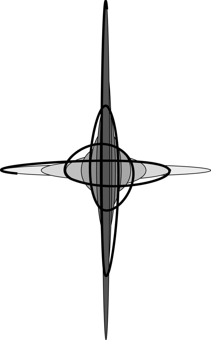
Figure 10. The universal cover of a manifold with a skew ${\mathbb{R}}$-covered Anosov foliation has an immersion in $\widetilde{T^{*}({\mathbb{H}}^{2})}$ that is invariant by the derivative action of a cocompact properly discontinuous subgroup of diffeomorphisms of the hyperbolic plane. In any fiber, the immersion would look something like this. There is a 1-parameter family of coaxial ellipses that describe the conformal structure of each leaf. The immersion is tangent to the unit ellipse for its hyperbolic metric.

Theorem 7.7.

The action of an extended convergence group on $\tilde{T}$ is conjugate to the action of a subgroup of $\widetilde{\mathop{\text{Diff}}}_{+}({\mathbb{H}}^{2})$ of uniformly Lipschitz diffeomorphisms on $\widetilde{\operatorname{TS}}^{*}({\mathbb{H}}^{2})$, where the action is the universal cover of the derivative. Conversely, any subgroup of the universal covering of the group of uniformly Lipschitz diffeomorphisms of ${\mathbb{H}}^{2}$ which acts properly discontinuously on $\widetilde{TS}^{*}({\mathbb{H}}^{2})$ is conjugate to an extended convergence group acting on $\tilde{T}$.

Furthermore, if $M$ is a closed $3$-manifold with a skew ${\mathbb{R}}$-covered Anosov foliation, then $\tilde{M}$ can be immersed in $T^{*}({\mathbb{H}}^{2})$ (probably not very smoothly), in a way that is invariant by the derivative of a representation of $\pi_{1}(M)$ in $\widetilde{\operatorname{Homeo}}({\mathbb{H}}^{2})$.

Proof.

Theorems 5.3 and 5.8 can be interpreted in the context of extended convergence groups, in the following form: Given an extended convergence group, we choose one of the three (isomorphic) slitherings, and apply theorem 5.8 or 5.3, to obtain a flow $\phi$ transverse to the foliation of the slithering. For present purposes, we just need a flow that serves as a connection for the slithering, so if necessary, we perturb $\phi$ to a flow $\phi^{\prime}$ that is a smooth and remains a connection.

We can now represent $Z$ by the homeomorphism having the required action on leaves of $\tilde{M}$, and isotopic to the identity along flow lines of $\phi^{\prime}$. This homeomorphism is likely not to be smooth, but it acts smoothly on the space of flow-lines. This gives a representation of $\pi_{1}(M)$ as a group of homeomorphisms of the universal cover of any leaf. We can lift this representation to the universal covering group of the group of homeomorphisms of the leaf, using the homotopy information that comes from the slithering, since the action on cotangent circles is the same up to homotopy with the action on the circle at infinity, which action is equipped with a lifting to an action on ${\mathbb{R}}$. ∎

8. Preview and questions

The circle at infinity for the leaves of a slithering is a particularly well-behaved instance of a general construction for a universal circle-at-infinity for the leaves of any taut foliation of a 3-manifold. In general, the universal circle can be thought of as defined by a foliation transverse to the fibers of $TS(\mathcal{F})$. It is not homeomorphic to the circles at infinity defined by the geometry of individual leaves. Instead, it is a collation of the circles for all leaves into one master circle: the circle at infinity for any particular leaf is obtained as a monotone (but not strictly monotone) image of the master circle. These universal circles will be constructed and analyzed in [Thu98] and they will be used to construct genuine essential laminations transverse to the leaves of any taut foliation of an atoroidal 3-manifold.

Harmonic measures for foliations constructed by Garnett ([Gar83]) are very helpful in understanding the geometry of leaves of taut foliations. They can be used to show that on any leaf $L$, in ‘most’ directions at infinity (in some sense, where the exact meaning of ‘most’ depends on $L$) the holonomy keeps a definite packet of nearby leaves within a bounded distance, and under many circumstances, makes them converge toward $L$. Anosov foliations are a particularly clear instance of this, where on any leaf, in all directions at infinity except one, the flow-lines diverge, but nearby leaves converge. The general picture is similar to this, except that there is often a dense set of exceptional directions where nearby leaves diverge. The exceptional set of directions has measure $0$ in any foliation such that every leaf is dense.

There has been a long history of a need for a widely-applicable geometric theory of universal Teichmüller space, that is, the space of hyperbolic structures on $D^{2}$ rel boundary, subject to some constraint on the geometry. This has been a key issue in studying iterated rational maps of the Riemann sphere, and it is also a key issue in the topology of three-manifolds. Of course, there are also many interesting unresolved issues concerning the geometry of ordinary finite-dimensional Teichmüller spaces.

I believe that three-manifolds that slither around $S^{1}$ provide a nice attainable testing ground, for refining some of our understanding about hyperbolic geometry and Teichmüller geometry. In general, given a compact space with a 2-dimensional lamination that has a hyperbolic leaves, one can study the Teichmüller space for the leaves—what are the possible hyperbolic metrics, up to isometry?

Associated with any lamination with 2-dimensional hyperbolic leaves, there is an associated 3-dimensional lamination with 3-dimensional hyperbolic leaves, modeled on ${\mathbb{H}}^{3}\supset{\mathbb{H}}^{2}$. The 3-dimensional laminations have interesting deformation spaces of their own; these are generalization of quasi-Fuchsian groups.

In the case of a lamination $\lambda$ embedded in a 3-manifold $M^{3}$, one can go further, and incorporate hyperbolic structures on the gaps into a foliation of 4-manifold $N^{4}$ with 3-dimensional hyperbolic leaves; $M^{3}$ is embedded in $N^{4}$ as a spine, in a way that leaves of the foliation of $N^{4}$ intersect $M^{3}$ as the leaves and gaps. (One should first blow up any isolated leaf of $\lambda$ to a band of parallel leaves, to make sure that $N^{4}$ will be Hausdorff.)

There are fairly natural ways to define a relaxation process on the deformation space of the 3-dimensional hyperbolic foliation, to try to bring nearby leaves isometrically closer. Actually, similar processes can be defined on the leaves of a foliated 3-manifold; some of these processes conjecturally should tend to a limit that is analogous to a geodesic in one of the metrics for Teichmüller space, yielding a transverse pseudo-Anosov flow under fairly general circumstances. (This would generalize ‘curve shortening’ as carried out by Bers in the special case of a surface fibration over $S^{1}$, [Ber78].)

I think it is likely that a relaxation process can be defined for the three-dimensional hyperbolic foliations that converges to give a geometric decomposition for $M$, usually by converging to a foliation where all leaves are actually isometric. What appears to happen is that as that an appropriate relaxation process makes the leaves ‘rotate’ in ${\mathbb{H}}^{3}\times$ Teichmüller space, so that the up and down ${\mathbb{H}}^{3}$-directions turn toward neighboring leaves above and below, ultimately converging to be isometric if the lamination is irreducible in the sense of not admitting transverse essential tori.

The case of a lamination consisting of a finite number of incompressible surfaces is simply a translation of a Haken manifold into this language, and the proofs for Haken manifolds show that the relaxation process converges in this case.

The next case will be 3-manifolds that slither around $S^{1}$. I am planning a paper to prove geometric convergence of a relaxation process defined in the pseudo-Anosov case by $(Z,Z^{-1})$. A key ingredient is that as one iterates, the quasi-isometric distance between leaves never increases, just as the ‘skinning maps’ decrease the Teichmüller metric in the Haken situation. In fact, because of the uniformness of the quasi-geometry of leaves in this situation, Curt McMullen’s proof of the Theta conjecture shows that distances between leaves actually contracts. Geometric estimates similar to previous cases will imply geometric convergence, yielding a hyperbolic structure for $M^{3}$. This scheme is a generalization of the construction for hyperbolic structures on mapping tori of pseudo-Anosov homeomorphisms.

I think it likely that further study will eventually show convergence (of some version of this process) in generality, for 3-manifolds with taut foliations or essential laminations.

Even more speculatively, the foliation pictures suggest a similar scheme that possibly could eventually yield a good natural proof for the general geometrization conjecture. The idea is to start with the unit tangent bundle, in some Riemannian metric, and turn the fibers into $3$-dimensional hyperbolic spaces. The aim is to look for a complete flat connection transverse to the fibers; the affine connection for the Riemannian metric gives a first approximation, but it is not a complete connection. In any case, the ${\mathbb{H}}^{3}$ foliation has a deformation theory parametrized by quasiconformal structures on its spheres. A relaxation process for this foliation can be defined, by making the conformal structure on the sphere at infinity evolve toward the shape of the spheres for its neighbors in the appropriate direction. The idea is something like ripples in a pond when a few equal-sized pebbles are dropped. The waves spread, perhaps becoming distorted from their initial conditions if the pond is shallow and irregular, but the wavefronts stay close to each other.

Three-manifolds with essential laminations are a special case of this general pebble-in-the-pond picture: 2-dimensional surfaces in a 3-manifold allow one to find a connection for the tangent ${\mathbb{H}}^{3}$-bundle that is integrable in two out of three directions, using Candel’s uniformization; in this case, relaxation needs to happen in is only one more direction.

There have been many powerful applications of foliations and laminations to analyzing 3-manifolds Dehn surgeries on knots. The phenomena in this paper suggest that there ought to be a theory which would connect surgeries along closed orbits of transverse pseudo-Anosov flows to rotation numbers and to the Milnor-Wood inequalities. One way to frame it is this: most surgeries along closed orbits of a pseudo-Anosov flow yield manifolds with pseudo-Anosov flows. For which surgeries is there a transverse foliation? For which surgeries does the flow uniformly regulate some transverse foliation? It seems a reasonable conjecture that every pseudo-Anosov flow is at least finitely covered by one that admits a transverse foliation. David Fried ([Fri83]) showed that any Anosov or pseudo-Anosov flow can be obtained by some Dehn surgery along flow lines of the suspension of a pseudo-Anosov homeomorphism of a surface. To do it, what is required is a section in the complement of some closed orbits, generalizing the Hedlund-Morse construction. A question related to generalizing the Milnor-Wood inequality is to describe the minimal collections of orbits that need to be removed for the flow to admit a section.

There are further related questions about tight contact structures: when is there a contact structure transverse to a flow, or tangential to a flow? These questions all seem closely linked. It would be nice to have a general theory of $\operatorname{Homeo}({\mathbb{R}})$-connections transverse to flows, or at least, for flows coming from slitherings of a 3-manifold over a surface; the ‘nicest’ cases are when the connection has positive or negative curvature, which gives a contact structure, or zero curvature, which gives a foliation. One can similarly look for analogues of the canonical 1-form in the cotangent bundle, that is, flows with plane fields (possibly with singularities) that twist positively, negatively, or not at all. See [ET97] for a discussion of related topics.

Similarly, what happens for surgeries along the leaves of a foliation (or of an essential lamination?) Is there a generalization of Fenley’s condition to some class of surgeries along the leaves of a 3-manifold that slithers around $S^{1}$?

Given a foliation transverse to the fibers of $M^{3}\times S^{1}$, is there some finite sheeted covering such that the pull-back bundle admits a transverse section (preferably defining a slithering)? The special case of the trivial question is the question of whether the three-manifold virtually fibers over $S^{1}$. It might be easier to do this when the foliated bundle is not trivial.

Is every hyperbolic three-manifold group isomorphic to a subgroup of $\operatorname{Homeo}{\mathbb{R}}$? This is beginning to seem likely.

In certain mysterious ways, foliations and essential laminations are quite similar to hyperbolic structures. Either kind of structure gives a positive and widely applicable criterion to show a manifold has many ‘nice’ properties including infinite fundamental group. On a surface, measured laminations can be thought of as the rank one limit of a conformal structure. A conformal class of indefinite metrics is a Lorentz cone structure. The canonical form for a diffeomorphism of a surface in essence produces one of the three types of conformal structures invariant by the diffeomorphism. Another way to think of the relationship is that hyperbolic structures are the same thing as grous acting on the complex $1$-manifold $\operatorname{\mathbb{CP}}^{1}$ that are ‘taut’ in a certain sense. This is the complex version of groups that act on $\operatorname{\mathbb{RP}}^{1}$. Foliations give groups acting on the circle, with many nice geometric properties.

One can only hope that some day, all these different structures and constructions will fit together into a single coherent picture.

References

- [Ber78] Lipman Bers. An extremal problem for quasiconformal mappings and a theorem by Thurston. Acta Math., 141(1-2):73–98, 1978.
- [Can93] Alberto Candel. Uniformization of surface laminations. Ann. Sci. École Norm. Sup. (4), 26(4):489–516, 1993.
- [CJ94] Andrew Casson and Douglas Jungreis. Convergence groups and Seifert fibered -manifolds. Invent. Math., 118(3):441–456, 1994.
- [CT85] James W. Cannon and William P. Thurston. Group invariant peano curves. Preprint, 1985.
- [EHN81] David Eisenbud, Ulrich Hirsch, and Walter Neumann. Transverse foliations of Seifert bundles and self homeomorphisms of the circle. Comment. Math. Helv., 56:638–660, 1981.
- [ET97] Yakov M. Eliashberg and William P. Thurston. Confoliations, volume 13 of University Lecture Notes in Mathematics. American Mathematical Society, Providence, 1997.
- [Far94] Benson Farb. Relative hyperbolic structures with applications to negatively curved manifolds. Princeton University Thesis, 1994.
- [Fen92a] Sérgio R. Fenley. Asymptotic properties of depth one foliations in hyperbolic -manifolds. J. Differential Geom., 36(2):269–313, 1992.
- [Fen92b] Sérgio R. Fenley. Quasi-isometric foliations. Topology, 31(3):667–676, 1992.
- [Fen94] Sérgio R. Fenley. Anosov flows in -manifolds. Ann. of Math. (2), 139(1):79–115, 1994.
- [Flo80] William J. Floyd. Group completions and limit sets of kleinian groups. Inventiones Mathematicae, 57(3):205–218, 1980.
- [Fri83] David Fried. Transitive Anosov flows and pseudo-Anosov maps. Topology, 22(3):299–303, 1983.
- [Gab92] David Gabai. Convergence groups are Fuchsian groups. Ann. of Math. (2), 136(3):447–510, 1992.
- [Gar83] Lucy Garnett. Foliations, the ergodic theorem and brownian motion. J. Funct. Anal., 51(3):285–311, 1983.
- [Ghy87] Étienne Ghys. Groupes d’homéomorphismes du cercle et cohomologie bornée. In The Lefschetz centennial conference, Part III (Mexico City, 1984), volume 58 of Contemp. Math., pages 81–106. Amer. Math. Soc., Providence, RI, 1987.
- [Gro87] M. Gromov. Hyperbolic groups. In Essays in group theory, volume 8 of Math. Sci. Res. Inst. Publ., pages 75–263. Springer, New York, 1987.
- [Har80] Detlef Hardorp. All Compact Orientable Three Dimensional Manifolds Admit Total Foliations. American Mathematical Society, Providence, 1980.
- [Mil58] John Milnor. On the existence of a connection with curvature zero. Comment. Math. Helv., 32:215–223, 1958.
- [Nov65] S.P. Novikov. Topology of foliations. Transactions of the Moscow Mathematical Society, 14:268–305, 1965.
- [Pal78] C. Palmeira. Open manifolds foliated by planes. Annals of Mathematics, 107:109–131, 1978.
- [Sch95] Richard Evan Schwartz. The quasi-isometry classification of rank one lattices. Inst. Hautes Études Sci. Publ. Math., 82:133–168 (1996), 1995.
- [Sul76] Dennis Sullivan. A generalization of Milnor’s inequality concerning affine foliations and affine manifolds. Comment. Math. Helv., 51(2):183–189, 1976.
- [Thu72] William P. Thurston. Foliations of 3-manifolds that are circle bundles. UCB Thesis, 1972.
- [Thu79] William P. Thurston. Geometry and Topology of Three-Manifolds. Princeton lecture notes, http://www.msri.org/gt3m, 1979.
- [Thu85] William P. Thurston. Minimal stretch maps between hyperbolic surfaces. Preprint, 1985.
- [Thu98] William P. Thurston. Three-manifolds, foliations and circles, II. Preprint in preparation, 1998.
- [Woo69] John W. Wood. Foliations on -manifolds. Ann. of Math. (2), 89:336–358, 1969.