Filling-Invariants at Infinity for Manifolds of Nonpositive Curvature

0. Introduction

Homological invariants “at infinity” and (coarse) isoperimetric inequalities are basic tools in the study of large-scale geometry (see e.g., [Gr]). The purpose of this paper is to combine these two ideas to construct a family $\mbox{div}_{k}(X^{n}),\ 0\leq k\leq n-2$, of geometric invariants for Hadamard manifolds $X^{n}$ . The $\mbox{div}_{k}(X^{n})$ are meant to give a finer measure of the spread of geodesics in $X^{n}$; in fact the 0-th invariant $\mbox{div}_{0}(X^{n})$ is the well-known “rate of divergence of geodesics” in the Riemannian manifold $X^{n}$.

The definition of $\mbox{div}_{k}(X^{n})$ goes roughly as follows (see Section 1 for the precise definitions): Find the minimum volume of a ball $B^{k+1}$ needed to fill a sphere $S^{k}$, where $S^{k}$ sits on the sphere $S(r)$ of radius $r$ in $X^{n}$, and the filling ball $B^{k+1}$ is required to lie outside the open ball $B(r)^{\circ}$ in $X^{n}$. Then $\mbox{div}_{k}(X^{n})$ measures the growth of this volume as $r\rightarrow\infty$; hence $\mbox{div}_{k}(X^{n})$ is in some sense a $k$-dimensional isoperimetric function at infinity.

We view the invariants $div_{k}(X^{n})$ in the same way as we view the standard isoperimetric inequalities (for manifolds or for groups): as basic geometric quantities to be computed.

The $\mbox{div}_{k}({X^{n}})$ are quasi-isometry invariants of $X^{n}$. The fundamental group $\pi_{1}(M^{n})$ (endowed with the word metric) of a compact Riemannian manifold is quasi-isometric to the universal cover $\widetilde{M^{n}}$; hence the $div_{k}(\widetilde{M^{n}})$ give quasi-isometry invariants for fundamental groups of closed, nonpositively curved manifolds $M^{n}$.

The contents of this paper are as follows: In Section 1, $div_{k}(X^{n})$ is defined and shown to be a quasi-isometry invariant. The core of this paper (Sections 2,3,4) describes three geometric techniques for computing $div_{k}(X^{n})$ for some basic examples. Section 4 also explores some surprising quasi-isometric embeddings hyperbolic spaces and solvable Lie groups into products of hyperbolic spaces.

We would like to express our gratitude to K. Fujiwara, C. Pugh, and A. Wilkinson for useful discussions, and to G. Kuperberg for doing the first two figures.

1. Definitions and Quasi-isometry Invariance

Let $X^{n}$ be a Hadamard manifold; that is, a complete, simply connected manifold all of whose sectional curvatures are nonpositive. Let $S(r)$, $B(r)$ and $B(r)^{\circ}$ denote respectively the sphere, ball and open ball of radius $r$ about a fixed basepoint $x_{0}$ of $X^{n}$, and let $C(r)\,=\,X^{n}\setminus B(r)^{\circ}$. Note that $C(r)$ deformation retracts onto the sphere $S(r)$; hence any continuous map $f:S^{k}\to S(r)$ admits a continuous extension, or filling $\widehat{f}:B^{k+1}\to C(r)$, for any integer $0\leq k\leq n-2$.

We shall be considering lipschitz maps to the manifold $X^{n}$. By the Whitney Extension Theorem, we know that if $f$ as above is lipschitz, then the extension $\widehat{f}$ of $f$ can be chosen to be lipschitz (with the same lipschitz constant). By Rademacher’s Theorem, lipschitz maps are differentiable almost everywhere, enabling one to define the $k$-volume of $f:S^{k}\to X^{n}$ and the $(k+1)$-volume of $\widehat{f}:B^{k+1}\to X^{n}$, where $S^{k}$ and $B^{k+1}$ denote the unit sphere and ball in euclidean space $\mbox{\bf R}^{n}$. More precisely, if the derivative $D_{x}f$ exists at a point $x\in S^{k}$, it sends an orthonormal basis at $x$ to a $k$-tuple of vectors in $T_{f(x)}(X^{n})$. We can comupte the $k$-volume of the parallelopiped spanned by this $k$-tuple using the metric on $X^{n}$. This defines a function $V(x)$ almost everywhere on $S^{k}$, and we can then define the $k$-volume of $f$, denoted $\mbox{\rm vol}_{k}(f)$, to be the integral of $V$ over $S^{k}$. This integral exists because $V(x)$ is a bounded measurable function defined almost everywhere on $S^{k}$, as $\|D_{x}f\|$ is bounded by the lipschitz constant of $f$.

We are now ready to define the invariant $\mbox{div}_{k}(X^{n})$ for a fixed integer $0\leq k\leq n-2$. Although the concept of $\mbox{div}_{k}$ is quite simple, the precise definition of $\mbox{div}_{k}$ needs to be somewhat technical in order to make it manifestly a quasi-isometry invariant. This is accomplished using a variation of a trick introduced in [Ge].

Let $A>0$ and $0<\rho\leq 1$ be given. For $r>0$, we define a map $f:S^{k}\to S(r)$ to be $A$-admissible if:

• $f$ is lipschitz, and

• $\mbox{\rm vol}_{k}(f)\leq Ar^{k}$

and say that the extension $\widehat{f}$ of $f$ is $\rho$-admissible if:

• $\widehat{f}$ is lipschitz, and

• $\widehat{f}(B^{k+1})\subset C(\rho r)$.

In other words, the only admissible fillings are those which lie outside the open ball $B^{\circ}(\rho r)$ in $X^{n}$. Now define

$$\delta^{k}_{\rho,A}(r)\;=\;\sup_{f}\inf_{\widehat{f}}\mbox{\rm vol}_{k+1}(\widehat{f})$$

where the supremun and infimum are taken over $A$-admissible maps $f$ and $\rho$-admissible fillings $\widehat{f}$ of $f$. We call the resulting two-parameter family of functions

$$\mbox{div}_{k}(X^{n})\;=\;\{\delta^{k}_{\rho,A}\;:\;0<\rho\leq 1,\;A>0\}$$

the $k$-th divergence of $X^{n}$ with respect to the point $x_{0}$. The parameters $\rho$ and $A$ are necessary in order to make $\mbox{\rm div}_{k}$ into a quasi-isometry invariant (see Theorem 1.1).

Remark: We note that the function $\delta^{k}_{\rho,A}(r)$, as a $\sup$ of an $\inf$, may not be realized by an actual filling, though of course there are (admissible) fillings arbitrarily close to realizing this function. We will ignore this distinction in what follows, as we are only interested in the growth of $\delta^{k}_{\rho,A}(r)$.

In this paper we shall only be concerned with distinguishing between polynomial and exponential functions. Hence the following equivalence relation: given functions $f,g:\mbox{\bf R}^{+}\rightarrow\mbox{\bf R}^{+}$, we write $f\preceq g$ if there exist constants $a,b,c>0$ and an integer $s\geq 0$ such that $f(x)\leq ag(bx)+cx^{s}$ for all sufficiently large $x$. Now write $f\sim g$ if both $f\preceq g$ and $g\preceq f$. This defines an equivalence relation on the class of functions from $\mbox{\bf R}^{+}\to\mbox{\bf R}^{+}$, and it makes sense to call the equivalence classes polynomial, exponential, super-exponential, etc.

Similarly, one defines an equivalence relation among $k$-th divergences as follows: say that $\mbox{\rm div}_{k}\preceq\mbox{\rm div}^{\prime}_{k}$ if there exist $0<\rho_{0},\rho^{\prime}_{0}\leq 1$ and $A_{0},A^{\prime}_{0}>0$ such that for every pair $(\rho,A)$ with $\rho<\rho_{0}$ and $A>A_{0}$ there exist $\rho^{\prime}<\rho^{\prime}_{0}$ and $A^{\prime}>A^{\prime}_{0}$ with $\delta^{k}_{\rho,A}\preceq{\delta^{\prime}}^{k}_{\rho^{\prime},A^{\prime}}$. Now define $\mbox{\rm div}_{k}\sim\mbox{\rm div}^{\prime}_{k}$ if we have both $\mbox{\rm div}_{k}\preceq\mbox{\rm div}^{\prime}_{k}$ and $\mbox{\rm div}^{\prime}_{k}\preceq\mbox{\rm div}_{k}$. In particular, we say that $\mbox{div}_{k}$ is polynomial or exponential, written $\mbox{div}_{k}=poly$ or $\mbox{div}_{k}=exp$, if there exists $0<\rho_{0}\leq 1$ and $0<A_{0}$ such that $\delta_{\rho,A}(r)\sim r^{d}$ (for some integer $d>0$) or $\delta_{\rho,A}(r)\sim e^{r}$ for all $\rho<\rho_{0}$ and $A>A_{0}$. Thus one can speak of polynomial or exponential $k$-th divergences.

We are now ready to prove that the invariants $div_{k}(X^{n})$ are actually quasi-isometry invariants of $X^{n}$, sometimes called geometric invariants. Recall that a quasi-isometry is basically a coarse bi-lipshitz map; these are the appropriate maps to study when one is interested in large-scale geometric properties of a space, or in geometric properties of the fundamental group of a compact Riemannian manifold (see, e.g., [Gr]). More precisely, we recall the following:

Definition: Let $X$ and $Y$ be metric spaces. A quasi-isometry is a pair of maps $f:X\longrightarrow Y,g:Y\longrightarrow X$ such that, for some constants $K,\epsilon,C>0$ :

$$\begin{array}[]{ll}d_{Y}(f(x_{1}),f(x_{2}))\leq Kd_{X}(x_{1},x_{2})+\epsilon,&d_{X}(g\circ f(x_{1}),x_{1})\leq C\\ d_{X}(g(y_{1}),g(y_{2}))\leq Kd_{Y}(y_{1},y_{2})+\epsilon,&d_{Y}(f\circ g(y_{1}),y_{1})\leq C\end{array}$$

for all $x_{1},x_{2}\in X,y_{1},y_{2}\in Y$. Note that neither $f$ nor $g$ need be continuous. If such maps exist, $X$ and $Y$ are said to be quasi-isometric; the map $f$ is called a $K$-quasi-isometry. A quasi-isometric embedding is defined similarly. A basic example to keep in mind is that the fundamental group $\pi_{1}(M)$ (endowed with the word metric) of a compact Riemannian manifold $M$ is quasi-isometric to the universal cover $\widetilde{M}$ of $M$.

Theorem 1.1 ($div_{k}$ is a quasi-isometry invariant).

The $k$-th divergence, $\mbox{\rm div}_{k}$, is a quasi-isometry invariant of Hadamard manifolds. In particular, $\mbox{\rm div}_{k}$ gives a quasi-isometry invariant for fundamental groups of closed, nonpositively curved manifolds.

Theorem 1.1 allows us to simply speak of the $k$-th divergence $div_{k}(X^{n})$ as “polynomial” or “exponential”, denoted by $\mbox{div}_{k}(X^{n})\sim exp$ and $\mbox{div}_{k}(X^{n})\sim poly$, respectively, without having to speak of the actual 2-parameter family of functions by which $div_{k}(X^{n})$ is defined. Whether $div_{k}(X^{n})$ is polynomial or exponential is then a quasi-isometry invariant notion.

Proof of Theorem 1.1: Let $F:(X,x_{0})\to(Y,y_{0})$ and $G:(Y,y_{0})\to(X,x_{0})$ be $L$-lipschitz maps between two based Hadamard manifolds which are determined by a quasi-isometry between $X$ and $Y$ (see Appendix A for existence of lipschitz quasi-isometries). We shall use these maps to compare the $k$-th divergences $\mbox{div}_{k}$ for $X$ and $\mbox{div}^{\prime}_{k}$ for $Y$.

Given an $A$-admissible map $f:S^{k}\to S_{X}(r)$, we can compose with $F$ to get a lipschitz map $F\circ f:S^{k}\to Y$ with $(F\circ f)(S^{k})\subset B_{Y}(Lr)\cap C_{Y}(r/L)$. Note that $\mbox{\rm vol}_{k}(F\circ f)\leq A(Lr)^{k}$. Radial projection onto $S_{Y}(r/L)$ defines a volume non-increasing lipschitz map (lipschitz constant 1) $\pi:C_{Y}(r/L)\to S_{Y}(r/L)$, and so the composition $(\pi\circ F\circ f):S^{k}\to S_{Y}(r/L)$ is $AL^{2k}$-admissible (see Figure 1). There is an admissible filling of this map with $(k+1)$-volume bounded by $\delta^{\prime k}_{\rho,A/L^{2k}}(r/L)$.

We obtain a lipschitz extension of $F\circ f$ as follows: on the radius one-half ball in $B^{k+1}$ take the map $(\widehat{\pi\circ F\circ f})\circ d_{2}$ where $d_{2}$ denotes the dilation taking the radius one-half ball $\frac{1}{2}B^{k+1}$ onto $B^{k+1}$, and on the remaining annular region just interpolate between the maps $F\circ f$ and $(\widehat{\pi\circ F\circ f})\circ d_{2}$ (sending radial geodesics in $B^{k+1}$ to geodesic segments between image points in $Y$). Note that the $(k+1)$-volume of this map is bounded by $\delta^{\prime}_{\rho,AL^{2k}}(r/L)$ plus a polynomial of degree $k+1$ in $r$. This polynomial bounds the $(k+1)$-volume of the annular region, and is the reason we use the equivalence relation among functions defined above.

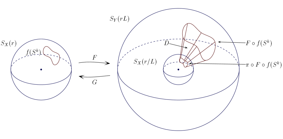
Figure 1. This figure illustrates part of the proof of Theorem 1.1.

Now postcomposition with $G$ yields a lipschitz map from $B^{k+1}$ to $X$ which lies outside the $\rho r/l^{2}$-ball about $x_{0}$, and the restriction of this map to $S^{k}$ is a constant distance (pointwise) away from the original map $f:S^{k}\to X$, as $G\circ F$ is a constant distance away from the identity map $1_{X}$. It is easy to see that one can interpolate between these maps to obtain a lipschitz map $\widehat{f}:B^{k+1}\to X$ which is a $\rho/L^{2}$-admissible filling of $f$. Note that

$$\mbox{vol}_{k+1}(\widehat{f})\,\leq\,L^{k+1}\delta^{\prime}_{\rho,AL^{2k}}(r/L)\,+\,p(r)$$

where $p(r)$ is a polynomial of degree $k+1$ in $r$, and so

$$\delta_{\rho/L^{2},A}(r)\preceq\delta^{\prime}_{\rho,AL^{2k}}(r)\,.$$

Thus, $\mbox{div}_{k}\preceq\mbox{div}^{\prime}_{k}$. Similarly, $\mbox{div}^{\prime}_{k}\preceq\mbox{div}_{k}$ and so $\mbox{div}_{k}$ is a true quasi-isometry invariant.

$\Box$

The proof of Theorem 1.1 shows that $\mbox{div}_{k}$ can be made more precise than $poly$ or $exp$; in fact, $\mbox{div}_{k}$ is a well-defined quasi-isometry invariant up to an additive factor of $x^{k+1}$.

2. Suspending Hard-to-Fill Spheres

In this section we show how to suspend hard-to-fill spheres in $X$ to hard-to-fill spheres in $X\times\mbox{\bf R}$. This provides a lower bound for the $(k+1)$st-divergence of $X\times\mbox{\bf R}$ in terms of the $k$th-divergence for $X$.

Theorem 2.1 (suspending hard-to-fill spheres).

Let $(X^{n},x_{0})$ be a based Hadamard manifold. Then

$$\mbox{div}_{k+1}(X^{n}\times\mbox{\bf R})\geq\mbox{div}_{k}(X^{n})\mbox{\ \ \ for any\ \ }0\leq k\leq n-3.$$

Theorem 2.1 shows, for example, that

$$\mbox{div}_{2}(\mbox{\bf H}^{2}\times\mbox{\bf R}^{2})\geq\mbox{div}_{1}(\mbox{\bf H}^{2}\times\mbox{\bf R})\geq\mbox{div}_{0}(\mbox{\bf H}^{2})\sim exp.$$

Proof of Theorem 2.1: Denote $X^{n}$ simply by $X$, and let $S(r)$ be the sphere of radius $r$ in $X\times\mbox{\bf R}$. Since $X=X\times\{0\}$ is totally geodesic in $X\times\mbox{\bf R}$, the intersection $S^{\prime}(r)=S(r)\cap X$ is the sphere of radius $r$ in $X$. Choose an admissible map $f:S^{k}\rightarrow S^{\prime}(r)$ which realizes $div_{k}(X)$. We now define a map

$$\Sigma(f):\Sigma(S^{k})=S^{k+1}\longrightarrow S(r)$$

where $\Sigma(S^{k})$ denotes the suspension $S^{k}\times[0,1]/((S^{k}\times\{0\})\cup(S^{k}\times\{1\}))$ of $S^{k}$. Geometrically, define the map $\Sigma(f)$ as follows: for $p\in S^{k}$, let $F_{p}$ be the 2-flat which is the product of the infinite geodesic in $X$ passing through $x_{0}$ and $f(p)$ and the infinite geodesic $\{x_{0}\}\times\mbox{\bf R}$. We think of each $F_{p}$ based at the “origin” $(x_{0},0)\in X\times\mbox{\bf R}$, and note that the points $x=(x_{0},r)$ and $y=(x_{0},-r)$ of $S(r)$ are contained in each $F_{p}$. Let $\gamma_{p}$ denote the arc of the circle of radius $r$ in $F_{p}$ from $x$ to $y$; this arc has length $\pi r$ (see Figure 2).

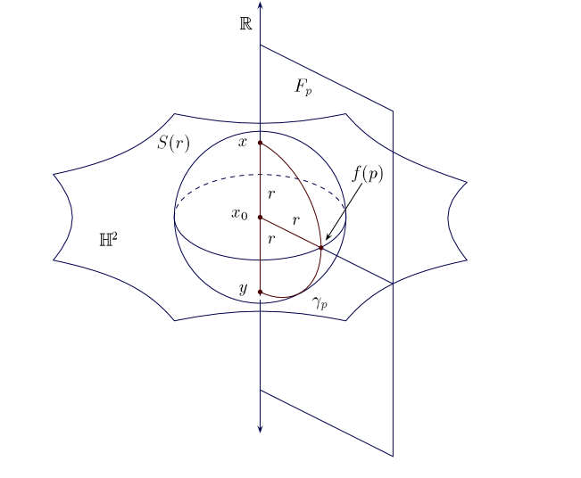
Figure 2. The arc $\gamma_{p}$ is used to define $\Sigma(f)$ at the point $\{p\}\times[0,1]$ of the suspension $\Sigma(S^{k})=S^{k+1}$.

Define the map $\Sigma(f)$ via:

$$\Sigma(f)(\{p\}\times[0,1])=\gamma_{p}.$$

So, for example, $\Sigma(f)$ stretches each $\{p\}\times[0,1]$ by a factor of $\pi r$. It is not difficult to check that $\Sigma(f):S^{k+1}\rightarrow S(r)$ is an admissible map. Note also that $\Sigma(f)(S^{k+1})\cap(X\times\{0\})=f(S^{k})$.

Suppose that $\widehat{\Sigma(f)}:B^{k+1}\rightarrow C(r)$ is an admissible filling of $\Sigma(f)$. Then $\widehat{\Sigma(f)}\cap(X\times\{0\})$ gives an admissible filling of $f(S^{k})$ in $X$, and this filling has volume at least $\delta^{k}(r)$, where $\delta^{k}(r)$ is the appropriate divergence function as in the definition of $div_{k}(X^{n})$.

Let a constant $\tau<<1$ be fixed. The reasoning above shows that for any $0\leq\epsilon\leq\tau$, the map given by $\widehat{\Sigma(f)}\cap(X\times\{\epsilon\})$ gives an admissible filling of $f(S^{k})$ in $X\times\{\epsilon\}$, and this filling has volume at least $\delta^{k}(r-\epsilon)$. Since the leaves $\{X\times\{\epsilon\}\}_{0\leq\epsilon\leq\tau}$ are parallel, we have

$$\begin{array}[]{ll}vol(\widehat{\Sigma(f)})&\geq\int_{0}^{\tau}\delta^{k}(r-\epsilon)d\epsilon\\ &\\ &\geq\int_{0}^{\tau}\delta^{k}(r-\tau)d\epsilon\\ &\\ &\geq\tau\cdot\delta^{k}(r-\tau)\\ &\\ &\sim\delta^{k}(r)\end{array}$$

as desired.

$\Box$

3. Pulling-Off Spheres Along Flats

In this section we give a polynomial upper bound for $div_{1}(X\times\mbox{\bf R}^{2})$ for any Hadamard manifold $X$ (Theorem 3.2). In order to do this we need the following, easily believable technical lemma. The main idea in the proof of Theorem 3.2 may be digested indpendently of the proof of this lemma.

Lemma 3.1 (homotoping off a neighborhood of the origin).

Let $\beta:S^{1}\rightarrow\mbox{\bf R}^{2}$ be a lipschitz map such that the length of $\beta(S^{1})$ is at most $Ar$. Then it is possible to homotope $\beta$ to $\beta^{\prime}:S^{1}\rightarrow\mbox{\bf R}^{2}$ of length at most $\pi Ar$, so that $\beta^{\prime}(S^{1})$ lies outside the open unit ball in $\mbox{\bf R}^{2}$. The paths $\beta$ and $\beta^{\prime}$ are homotopic by a lipschitz homotopy of area at most $2\pi Ar$.

Proof: Let $B^{\circ}$ and $\partial B$ denote respectively the open unit ball and unit circle in $\mbox{\bf R}^{2}$. The map $\beta$ is lipschitz and therefore continuous, and so $\beta^{-1}(B^{\circ})$ is an open subset of $S^{1}$. There are three cases to consider.

In the first case $\beta^{-1}(B^{\circ})=\emptyset$, and we take $\beta^{\prime}=\beta$ and the result is trivial.

In the second case $\beta^{-1}(B^{\circ})=S^{1}$. Here we take $\beta^{\prime}=\tau_{\vec{v}}\circ\beta$ where $\tau_{\vec{v}}:\mbox{\bf R}^{2}\to\mbox{\bf R}^{2}$ is just translation by a vector $\vec{v}$ of length 2. The homotopy is given by maps $\tau_{t\vec{v}}\circ\beta$ where $t\in[0,1]$. Since the $\tau_{t\vec{v}}$ are isometries of $\mbox{\bf R}^{2}$ in the Euclidean metric, $\beta^{\prime}$ is lipschitz of length $Ar$, and the homotopy is clearly lipschitz, of area at most $2Ar$.

Finally, $\beta^{-1}(S^{1})$ may be a non-empty proper open subset of $S^{1}$, and so is the disjoint union of a collection of open intervals in $S^{1}$. Given such an open interval $(a,b)\subset S^{1}$, we may define $\beta^{\prime}|_{[a,b]}$ to agree with $\beta$ on the endpoints $a$ and $b$, and to map $[a,b]$ uniformly over the smaller of the arcs of $\partial B$ determined by $\beta(a)$ and $\beta(b)$ (either arc if $\beta(a)$ and $\beta(b)$ are antipodal). We take the straight line homotopy $t\beta^{\prime}(x)+(1-t)\beta(x)$ in $\mbox{\bf R}^{2}$, between $\beta$ and $\beta^{\prime}$. It is clear from the construction that $\beta^{\prime}$ and the homotopy are lipschitz, and that the length of $\beta^{\prime}$ is bounded by $\pi Ar$, and that the area of the homotopy is at most $2\pi Ar$. $\Box$

Theorem 3.2 (a polynomial filling).

Let $X$ be a Hadamard manifold. Then

$$\mbox{div}_{1}(X\times\mbox{\bf R}^{2})$$

is polynomial of degree three.

Proof: Let an $A$-admissible map $\gamma:S^{1}\rightarrow S(r)$ be given, where $S(r)$ is the sphere of radius $r$ around a chosen basepoint $x_{0}\in X$. Let $\pi:X\times\mbox{\bf R}^{2}\rightarrow\mbox{\bf R}^{2}$ be the natural projection.

From Lemma 3.1 applied to $\beta=\pi\circ\gamma$, it is clear that we may homotope $\gamma$ slightly so that $\pi\circ\gamma(S^{1})$ lies outside the open unit ball in $\mbox{\bf R}^{2}$. An admissible filling of this perturbed $\gamma$ then gives an admissible filling of $\gamma$. Since the area of these two maps differs by at most some constant (not depending on $r$) times $r$, we may assume without loss of generality that $\pi\circ\gamma(S^{1})$ lies outside the open unit ball in $\mbox{\bf R}^{2}$.

We now give an admissible filling $\hat{\gamma}:B^{2}\rightarrow C(r)$ of $\gamma$. The filling is given by the tracks of $\gamma$ under a sequence of 4 homotopies which homotope $\gamma$ (outside $B(r)$) to a point; this filling is illustrated in Figure 3.

Figure 3. This figure gives a sequence of 4 homotopies which homotope $\gamma$ (outside $B(r)$) to a point. The homotopy is illustrated by its projections onto the $X$ and $\mbox{\bf R}^{2}$ factors.

Here is the sequence of homotopies :

1. Radial projection in the $\mbox{\bf R}^{2}$ factor to the $3r$-sphere in $\mbox{\bf R}^{2}$: $(x,\vec{v})\mapsto(x,t\cdot\frac{\vec{v}}{||\vec{v}||}),1\leq t\leq 3r$. Since $\pi\circ\gamma$ lies outside the open unit ball in $\mbox{\bf R}^{2}$, this radial projection is well-defined, and increases the length of $\gamma$ by at most a factor of $3r$ (hence the length of the image of $\gamma$ under this radial projection is at most $3r\cdot|\gamma|\leq 3Ar^{2}$).

2. Coning-off in the $X$ factor: $(x,\vec{v})\mapsto(\sigma_{x}(t),\vec{v}),0\leq t\leq 1$, where $\sigma_{x}$ is the (unique) geodesic in $X$ from $x$ to $x_{0}$.

3. Pulling to the $5r$-sphere in the $X$ factor: $(x_{0},\vec{v})\mapsto(\tau(t),\vec{v}),0\leq t\leq 1$, where $x_{1}$ is any (fixed) point lying on the sphere of radius $5r$ in $X$, and $\tau$ is the unique geodesic from $x_{0}$ to $x_{1}$.

4. Coning-off in the $\mbox{\bf R}^{2}$ factor: $(x_{1},\vec{v})\mapsto(x_{1},(1-t)\cdot\vec{v}),0\leq t\leq 1$.

It is easy to check that the images of these homotopies lies outside $B(r)$, since the metric on $X\times\mbox{\bf R}^{2}$ is just the product metric. Piecing together these homotopies gives a map $\gamma^{\prime}:S^{1}\times[0,1]\rightarrow C(r)$ with the image $\gamma^{\prime}(S^{1}\times\{1\})$ being the point $(x_{1},\vec{0})$; hence this induces a map on the cone on $S^{1}$, that is a map $\hat{\gamma}:B^{2}\rightarrow C(r)$. The map $\hat{\gamma}$ is easily seen to be an admissible filling of area at most

$$(3Ar^{2})\cdot(3r)+(Ar)\cdot r+(3Ar^{2})\cdot(5r)+(3Ar^{2})\cdot(3r)\leq 35Ar^{3}.$$

Hence $div_{k}(X\times\mbox{\bf R}^{2})$ is (equivalent to) a polynomial of degree $3$. $\Box$

Remark: It is probably true, more generally, that $div_{k}(X\times\mbox{\bf R}^{m})$ is polynomial for $k<m$. The proof of Theorem 3.2 works verbatim in this case, except for Lemma 3.1 (which we believe to be true, although we have not been able to find a proof).

4. Transverse Flats and Hyperbolic Spaces in Products

It is a surprising (but not difficult to see) fact that there is, for example, a quasi-isometrically embedded copy of $\mbox{\bf H}^{3}$ inside $\mbox{\bf H}^{2}\times\mbox{\bf H}^{2}$ . In the first part of this section, we show that there are quasi-isometric embeddings of hyperbolic spaces and solvable Lie groups in products of hyperbolic spaces, although these embeddings are not quasi-convex. We then apply the first embeddings to find a lower bound for certain $\mbox{div}_{k}$ of products of hyperbolic spaces.

The idea is to exploit the fact that, in a product of hyperbolic spaces $X$, there is a flat and a nicely embedded hyperbolic space whose dimensions add to $dim(X)+1$. The flat is used to find a polynomial-volume sphere; the hyperbolic space is used to show that any admissible filling of this sphere has exponential volume.

Recall that a subset $Y$ of a metric space $X$ is called quasiconvex in $X$ if there is a constant $D\geq 0$ so that any geodesic in $X$ between points $y_{1},y_{2}\in Y$ lies in the $D$-neighborhood of $Y$.

Proposition 4.1 (q.i. embeddings).

There are quasi-isometric embeddings of

$$\mbox{\bf H}^{(m_{1}\,+\,\cdots\,+\,m_{n})\,-\,k+1}$$

and of an $((m_{1}+\cdots+m_{n})-k+1)$-dimensional solvable Lie group in $X=\mbox{\bf H}^{m_{1}}\times\cdots\times\mbox{\bf H}^{m_{k}}$, where each $m_{i}>1$. These embeddings are not quasiconvex.

Examples: Proposition 4.1 shows that there are quasi-isometrically embedded (but not quasiconvex) copies of $\mbox{\bf H}^{3}$ and of the three-dimensional geometry Sol in $\mbox{\bf H}^{2}\times\mbox{\bf H}^{2}$, and that there are quasi-isometrically embedded copies of $\mbox{\bf H}^{4}$ in $\mbox{\bf H}^{2}\times\mbox{\bf H}^{2}\times\mbox{\bf H}^{2}$ and of $\mbox{\bf H}^{5}$ in $\mbox{\bf H}^{3}\times\mbox{\bf H}^{3}$.

Proof: Let $\gamma(t)=(\gamma_{1}(t),\ldots,\gamma_{k}(t))$ be an infinite diagonal geodesic in $X$, parameterized by arc length; so that $\gamma_{i}$ traces out (at a speed of $1/{\sqrt{k}}$ times unit speed) an infinite geodesic $g_{i}$ in $H^{m_{i}}$. For each $1\leq i\leq k$, let $S_{i}^{+}(t)$ (respectively $S_{i}^{+}(t)$) denote the horosphere in $\mbox{\bf H}^{m_{i}}$ which is centered at $\gamma_{i}(+\infty)$ (respectively $\gamma_{i}(-\infty)$) and which contains the point $\gamma(t)$.

Now we define the quasi-isometrically embedded copy of hyperbolic space

$$Y\;=\;\mbox{\bf H}^{(m_{1}+\cdots+m_{k})-k+1}\;=\;\mbox{\bf R}^{(m_{1}+\cdots+m_{k})-k}\times\nobreak\kern-1.90002pt\rule{0.25pt}{4.73611pt}\,\mbox{\bf R}$$

in $\mbox{\bf H}^{m_{1}}\times\cdots\times\mbox{\bf H}^{m_{k}}$ to be the set of points

$$\{(x_{1},\ldots,x_{k})\;:\;x_{i}\in S_{i}^{+}(t)\;,\;t\in\mbox{\bf R}\}$$

Note that this set contains the geodesic $\gamma$ which is the vertical R in
$\mbox{\bf R}^{(m_{1}+\cdots+m_{k})-k}\times\nobreak\kern-1.90002pt\rule{0.25pt}{4.73611pt}\,\mbox{\bf R}$. Each horosphere $S_{i}$ contributes a copy of $\mbox{\bf R}^{m_{i}-1}$ which is scaled by a factor of $e^{-t/{\sqrt{k}}}$. Hence the metric induced on
$\mbox{\bf R}^{(m_{1}+\cdots+m_{k})-k}\times\nobreak\kern-1.90002pt\rule{0.25pt}{4.73611pt}\,\mbox{\bf R}$ is given by

$$dt^{2}\,\,+e^{-t/{\sqrt{k}}}ds^{2}$$

where $ds^{2}$ denotes the Euclidean metric on $\mbox{\bf R}^{(m_{1}+\cdots+m_{k})-k}$.

Figure 4. The hyperbolic space is quasi-isometrically embedded.

First we show that $Y\subset X$ is a quasi-isometric embedding. For any two points $p,q\in Y$ we have $d_{X}(p,q)\leq d_{Y}(p,q)$. For the rest of the proof we refer to Figure 4. Let $p_{i}$ and $q_{i}$ denote the projections of $p$ and $q$ onto the factors $\mbox{\bf H}^{m_{i}}$, and let $\gamma_{i}$ denote the geodesic in $\mbox{\bf H}^{m_{i}}$ between $p_{i}$ and $q_{i}$. Since $p,q\in Y$, the $p_{i}$ all have the same vertical coordinate $t$ and the $q_{i}$ all have the same vertical coordinate $t^{\prime}$.

For each $1\leq i\leq k$ let

$$\pi_{i}:\mbox{\bf H}^{m_{i}}\to g_{i}:(x_{1},\ldots,x_{m_{i}},t)\mapsto t$$

denote the horospherical projection onto the vertical geodesic $g_{i}$, and let

$$\tau\,=\,\sup_{i}\mbox{length}(\pi_{i}(\gamma_{i}))\,.$$

Denote by $a_{i}$ and $b_{i}$ respectively, the points in $\mbox{\bf H}^{m_{i}}$ which lie vertically above $p_{i}$ and $q_{i}$ on the horospherical level $\min\{t,t^{\prime}\}\,+\,\tau$.

Now consider the path in $Y$ from $p$ to $q$ which consists of the diagonal geodesic segments from $p=(p_{i},\ldots,p_{k})$ to $(a_{i},\ldots,a_{k})$ and from $(b_{1},\ldots,b_{k})$ to $q=(q_{1},\ldots,q_{k})$, and a geodesic (in the intinsic metric on the product of horospheres $S_{1}^{+}\times\cdots\times S_{k}^{+}$) from $(a_{1},\ldots,a_{k})$ to $(b_{1},\ldots,b_{k})$. Each of the diagonal geodesics have length bounded by $\sqrt{k}\tau$ and the other geodesic segment has length with bound $2\sqrt{k}$.

Thus the length of this path is less than $2\sqrt{k}\tau+2\sqrt{k}$ and so we have

$$d_{Y}(p,q) \leq 2\sqrt{k}\tau+2\sqrt{k}$$

$$\leq 2\sqrt{k}d_{\mbox{\bf H}^{m_{j}}}(p_{j},q_{j})+2\sqrt{k}$$

$$\leq 2\sqrt{k}d_{X}(p,q)+2\sqrt{k}$$

where $\mbox{\bf H}^{m_{j}}$ is the factor realizing the maximum of the lengths of $\pi_{i}(\gamma_{i})$.

Now we show that $Y$ is not quasi convex in $X$. Consider the two points $(p_{1},p_{2},\ldots,p_{k})$ and $(q_{1},p_{2},\ldots,p_{k})$ in $Y$ where $p_{1}$ and $q_{1}$ lie on the same horosphere in $\mbox{\bf H}^{m_{1}}$. The $X$ geodesic between these points is just the geodesic in $\mbox{\bf H}^{m_{1}}$ from $p_{1}$ to $q_{1}$ (with the other coordinates just constant at the point $(p_{2},\ldots,p_{k})$). Clearly this does not lie in $Y$; in fact, the distance from its midpoint $(r_{1},p_{2},\ldots,p_{k})$ to $Y$ is given by

$$\min_{l_{1}+l_{2}=l}\sqrt{(k-1)l_{1}^{2}+l_{2}^{2}}$$

where $l$ is the vertical height of the geodesic between $p_{1}$ and $q_{1}$ in $\mbox{\bf H}^{m_{1}}$. This can be made arbitrarily large by choosing $p_{1}$ and $q_{1}$ far apart.

Finally, note that there are quasi isometrically embedded copies of solvable Lie groups in $X$; these are just the horospheres in $X$. More explicitly, for example, define $Z$ in $X$ to be the set of points

$$Z\;=\;\{(x_{1},\ldots,x_{k})\;:\;x_{1}\in S^{+}_{1}(t)\,,\;x_{i}\in S^{-}_{i}(t)\;\;(i=2,\ldots,k)\,,\;t\in\mbox{\bf R}\}$$

We leave it to the reader to verify that the induced metric on $Z\;=\;\mbox{\bf R}^{(m_{1}\,+\,\cdots\,+\,m_{k})\,-\,k}\times\nobreak\kern-1.90002pt\rule{0.25pt}{4.73611pt}\,\mbox{\bf R}$ is given by

$$dt^{2}+\,e^{-t/\sqrt{k}}ds_{1}^{2}+e^{t/\sqrt{k}}ds_{2}^{2}$$

where $ds_{1}^{2}$ denotes the Euclidean metric on $\mbox{\bf R}^{m_{1}-1}$ and $ds_{2}^{2}$ denotes the Euclidean metric on $\mbox{\bf R}^{(m_{2}+\cdots+m_{k})-k+1}$, and that $Z$ is quasi isometrically embedded in $X$. $\Box$

The geodesic $\gamma$ of Proposition 4.1 is contained in the $k$-flat $F=\gamma_{1}\times\cdots\times\gamma_{k}$. This $k$-flat is foliated by parallel geodesics of the form

$$\gamma_{(s_{1},\ldots,s_{k})}(t)\;=\;(\gamma_{1}(t+s_{1}),\ldots,\gamma_{k}(t+s_{k}))$$

where $s_{1}+\cdots+s_{k}=0$. The corresponding family of hyperbolic spaces

$$Y_{(s_{1},\ldots,s_{k})}\;=\;\{(x_{1},\ldots,x_{k})\;:\;x_{i}\in S^{+}_{i}(t+s_{i})\,,\;\;t\in\mbox{\bf R}\}$$

gives a codimension $(k-1)$ foliation of $X$, where each $Y_{(s_{i},\ldots,s_{k})}$ intersects the $k$-flat $\gamma_{1}\times\cdots\times\gamma_{k}$ in the geodesic $\gamma_{(s_{1},\ldots,s_{k})}$.

Lemma 4.2.

For any points $p\in Y_{(s_{1},\ldots,s_{k})}$ and $q\in Y_{(s^{\prime}_{1},\ldots,s^{\prime}_{k})}$ we have

$$d_{X}(p,q)\;\geq\;\sqrt{(s_{1}-s^{\prime}_{1})^{2}\,+\,\cdots\,+\,(s_{k}-s^{\prime}_{k})^{2}}$$

Proof: Perpendicular projection of $X$ onto the $k$-flat $\gamma_{1}\times\,\cdots\,\times\gamma_{k}$ is a distance nonincreasing map which takes $p$ and $q$ to points on the geodesic lines $\gamma_{(s_{1},\ldots,s_{k})}$ and $\gamma_{(s^{\prime}_{1},\ldots,s^{\prime}_{k})}$ respectively. The $X$-distance between the image points is the same as the distance in the $k$-flat, which is bounded below by $\sqrt{(s_{1}-s^{\prime}_{1})^{2}\,+\,\cdots\,+\,(s_{k}-s^{\prime}_{k})^{2}}$. $\Box$

Theorem 4.3 (some hard-to-fill spheres).

Let $X=\mbox{\bf H}^{m_{1}}\times\cdots\times\mbox{\bf H}^{m_{k}}$, each $m_{i}>1$, be a product of $k$ hyperbolic spaces. Then $\mbox{div}_{k-1}(X)=exp$.

Proof: Consider the family of hyperbolic spaces $\{Y_{s}\}$ as above, where $s\in B(1)$, the ball of radius 1 in $F$. Recall that $F=\gamma_{1}\times\cdots\times\gamma_{k}$ is a totally geodesic, isometrically embedded copy of $\mbox{\bf R}^{k}$ in $X$. Also recall that the volume of a sphere of radius $r$ in $\mbox{\bf R}^{k}$ is $ar^{k}$ for some constant $a$ depending only on $k$.

Now let $A>a$ and $r>0$ be given, and let $T=F\cap S(r)$. Then $T$ is a $(k-1)$-dimensional sphere lying on the sphere $S(r)$ of radius $r$ about the origin in $X$. Since $T\subset F$ and $F$ is a flat in $X$, we have $vol_{k-1}(T)\leq ar^{k}\leq Ar^{k}$. We claim that any filling of $T$ outside of $S(r)$ has $(k+1)$-volume on the order of $e^{r}$.

To prove this claim, suppose that $\widehat{T}$ is an admissible filling of $T$. First note that the intersection $T\cap Y_{s}$ in $X$ has dimension 0; in fact, $T\cap Y_{s}$ consists precisely of the two points $T\cap\gamma_{s}=\{x_{s},y_{s}\}$. Since $x_{s}$ and $y_{s}$ are each within a distance of 1 from antipodal points of $S(R)$ lying on the geodesic $\gamma_{0}$, it follows that $x_{s}$ and $y_{s}$ are each within a distance of 1 from antipodal points on the sphere $S^{\prime}(r)$ of radius $r$ in $Y$. Now $\widehat{T}\cap Y_{s}$ is a one-dimensional arc in $Y_{s}$ which connects $x_{s}$ to $y_{s}$ outside of $S^{\prime}(r)$. Since $Y_{s}$ is a hyperbolic space, $\mbox{div}_{0}(Y_{s})$=exp, so that the arc $\widehat{T}\cap Y_{s}$ has length at least $Ce^{r}$ for some constant $C$ which is independent of $r$. We note that since $s\in B(1)$, the constant $C$ may be chosen to work for all $Y_{s}$.

Now

$$\begin{array}[]{lll}vol_{k+1}(\widehat{T})&=\int_{B(1)}vol_{k+1}(\widehat{T}\cap Y_{s})d\mu(s)&\\ &&\\ &\geq\int_{B(1)}Ce^{r}d\mu(s)&\mbox{since $|\widehat{T}\cap Y_{s}|\geq Ce^{r}$}\\ &&\\ &\geq Ce^{r}\mu(B(1))&\mbox{by Lemma \ref{stackofh}}\end{array}$$

and we are done.

$\Box$

Remark: The reason it is necessary to use Lemma 4.2 is that it is possible to have, for example, a disc foliated by an interval’s worth of lines of length $e^{r}$, but with the area of the disc being constant. For example consider a long, thing quadrilateral in the hyperbolic plane: it is foliated by lines of length $e^{r}$ for $r$ large, but it’s area is bounded by a universal constant; the reason is that the leaves of the foliation are bent so that they come very close together, on the order of $e^{-r}$, in fact.

5. Questions

As stated above, we view the invariants $div_{k}(X)$ as basic geometric quantities to be computed. We believe that the invariants $\mbox{div}_{k}(X^{n})$ are computable for many more examples than are covered in this paper.

Question: Compute $\mbox{div}_{k}(X)$ for symmetric spaces $X$ of noncompact type. The simplest case not covered in this paper is $\mbox{div}_{2}(\mbox{\bf H}^{2}\times\mbox{\bf H}^{2})$. We believe that $div_{1}(X)\sim e^{r}$ for the symmetric space $X=SL_{n}(\mbox{\bf R})/SO_{n}(\mbox{\bf R})$.

Question: Can the invariants $div_{k}(X)$ be used to detect the rank of a (globally) symmetric space $X$ of noncompact type?

Appendix A

In this appendix we give a technical proposition which was needed to show that the $div_{k}(X^{n})$ are quasi-isometry invariants.

Proposition A.1: Suppose $f:X\rightarrow Y$ is a quasi-isometry between Hadamard manifolds, and suppose that $X$ admits a cocompact lattice. Then $f$ is a bounded distance from a (continuous) lipshitz map $f^{\prime}:X\rightarrow Y$; that is, $sup_{x\in X}d_{Y}(f(x),f^{\prime}(x))\leq C$ for some constant $C>0$.

Proof: Since $X$ admits some compact quotient $M=X/{\Gamma}$, it is possible to lift a triangulation of $M$ to to a $\Gamma$-equivariant triangulation of $X$. Note that there are finitely isometry types of simplices in this triangulation of $X$.

The map $f^{\prime}$ is defined inductively on the skeleta of the triangulation. On vertices we simply define $f^{\prime}$ to equal $f$. Suppose $f^{\prime}$ is defined on the $k$-skeleton of the triangulation; then for each $(k+1)$-simplex $\sigma$, we have a Lipshitz map defined on $\partial(\sigma)$, which is a sphere. This map extends to a lipshitz map on $\sigma$ by Whitney’s Extension Theorem. Do this for each different $(k+1)$-simplex $\sigma$; the point is that there are only finitely many different lipshitz constants since there are only finitely many isometry types of simplices; hence the map $f^{\prime}$ is lipshitz with constant the maximum of the Whitney lipshitz constants on the finitely many isometry types of simplices. $\Box$

References

- [Ge] S.M. Gersten, Quadratic divergence of geodesics in spaces, Geometric and Functional Analysis, Vol.3, No.6 (1993).
- [Gr] M. Gromov, Asymptotic Invariants of Infinite Groups, in Geometric Group Theory, G. Niblo and M. Roller, eds., LMS Lecture Notes 182, Cambridge Univ. Press, 1993.