Dynamics of quadratic polynomials:
Complex bounds for real maps

Abstract.

We extend Sullivan’s complex a priori bounds to real quadratic polynomials with essentially bounded combinatorics. Combined with the previous results of the first author, this yields complex bounds for all real quadratics. Local connectivity of the corresponding Julia sets follows.

1. Introduction

Complex a priori bounds proved to be a key issue of the Renormalization Theory. They lead to rigidity results, local connectivity of Julia sets and the Mandelbrot set, and convergence of the renormalized maps (see [HJ, L3, McM1, MvS, R, S]).

By definition, this property means that the renormalized maps $R^{n}f$ have fundamental annuli with a definite modulus. For real infinitely renormalizable maps with bounded combinatorics this property was proven by Sullivan ( see [S] and [MvS] ). In [L3] complex bounds were proven for real quadratics of “essentially big type”. The gap in between [S] and [L3] consists of maps with “essentially bounded type”. Loosely speaking this means that a big period of renormalized maps is created only by saddle-node behavior of the return maps. The goal of this paper is to analyze this specific phenomenon.

Theorem 1.1.

Real infinitely renormalizable quadratics with essentially bounded combinatorics have complex a priori bounds.

This fills the above mentioned gap:

Corollary 1.2.

All infinitely renormalizable real quadratics have complex a priori bounds.

Let us mention here only one consequence of this result. By the result of Hu and Jiang [HJ, J], complex a priori bounds and one extra combinatorial assumption (see [McM2]) imply local connectivity of the Julia set $J(f)$. On the other hand, the Yoccoz Theorem gives local connectivity of $J(f)$ for at most finitely renormalizable quadratic maps (see [H], [L1] or [M1]). Thus we have

Corollary 1.3.

The Julia set of any real quadratic map is locally connected.

Theorem 1.2 is closer to [S] rather than [L3]. It turns out, however, that Sullivan’s Sector Lemma (see [MvS]) is not valid for essentially bounded (but unbounded) combinatorics: The pullback of the plane with two slits is not necessarily contained in a definite sector. What turns out to be true instead is that the little Julia sets $J(R^{n}f)$ are contained in a definite sector.

We derive this version of the Sector Lemma from the following quadratic estimate for the renormalized maps:

(1.1) $$|R^{n}f(z)|\geq c|z|^{2},$$

with an absolute $c>0$. The proof of (1.1) is the main technical concern of this work. (By the way, this estimate immediately implies that the little Julia sets $J(R^{n}f)$ are commensurable with the corresponding periodic intervals, which already yields local connectivity of $J(f)$ at the critical point.)

Let $\mod(f)$ denote the supremum of the moduli of the fundamental annuli of $f$. The work [L3] gives a criterion when $\mod(Rf)$ is big. Let us call the combinatorial parameter responsible for this the essential period $p_{e}(f)$. Loosely speaking this is the period of the corresponding periodic interval of $f$ modulo the saddle-node cascades (see §5 for the precise definition).

Corollary 1.4.

There is an absolute constant $\gamma>0$ and two functions $\mu(p)>\nu(p)>\gamma>0$ going to $\infty$ as $p\to\infty$ with the following property. Let $f$ be an infinitely renormalizable quadratic polynomial and $p_{n}=p_{e}(R^{n}f)$. Then

$$\nu(p_{n})\leq\mod(R^{n}f)\leq\mu(p_{n}).$$

Let us briefly outline the structure of the paper. §2 contains some background and technical preliminaries. In §3 we state the main technical lemmas, and derive from them our results. In §4 we give a quite simple proof of complex bounds in the case of bounded combinatorics, which will model the following argument. In §5 essentially bounded combinatorics is described. In the next section, §6, saddle-node cascades are analyzed. The final section, §7, contains the proof of the main technical lemmas.

Remark 1. Theorem 1.1 allows a straightforward extension onto higher degree unimodal polynomials.

2. This paper is a part of series of notes on dynamics of quadratic polynomials, see [L4].

Acknowledgment. The authors thank MSRI where part of this work was done for its hospitality.

2. Preliminaries

2.1. General notations and terminology

We use $|J|$ for the length of an interval $J$, $\operatorname{dist}$ and $\operatorname{diam}$ for the Euclidean distance and diameter in $\mathbb{C}$. Notation $[a,b]$ stands for the (closed) interval with endpoints $a$ and $b$ without specifying their order.

Two sets $X$ in $Y$ in $\mathbb{C}$ are called $K$-commensurable or simply commensurable if

$$K^{-1}\leq\operatorname{diam}X/\operatorname{diam}Y\leq K$$

with a constant $K>0$ which may depend only on the specified combinatorial bounds.

We say that an annulus $A$ has a definite modulus if $\mod A\geq\delta>0$, where $\delta$ may also depend only on the specified combinatorial bounds.

For a pair of intervals $I\subset J$ we say that $I$ is contained well inside of $J$ if for any of the components $L\subset J\setminus I$, $|L|\geq K|I|$ where the constant $K>0$ may depend only on the specified quantifiers.

A smooth interval map $f:I\rightarrow I$ is called unimodal if it has a single critical point, and this point is an extremum. A $C^{3}$ unimodal map is called quasi-quadratic if it has negative Schwarzian derivative, and its critical point is non-degenerate.

Given a unimodal map $f$ and a point $x\in I$, $x^{\prime}$ will denote the dynamically symmetric point, that is, such that $fx^{\prime}=fx$. Notation $\omega(z)$ means as usual the limit set of the forward orbit $\{f^{n}z\}_{n=0}^{\infty}$.

2.2. Hyperbolic disks

Given an interval $J\subset\mathbb{R}$, let $\mathbb{C}_{J}\equiv\mathbb{C}\backslash(\mathbb{R}\backslash J)$ denote the plane slit along two rays. Let ${\bar{\mathbb{C}}}_{J}$ denote the completion of this domain in the path metric in $\mathbb{C}_{J}$ (which means that we add to $\mathbb{C}_{J}$ the banks of the slits).

By symmetry, $J$ is a hyperbolic geodesic in $\mathbb{C}_{J}$. The geodesic neighborhood of $J$ of radius $r$ is the set of all points in $\mathbb{C}_{J}$ whose hyperbolic distance to $J$ is less than $r$. It is easy to see that such a neighborhood is the union of two $\mathbb{R}$-symmetric segments of Euclidean disks based on $J$ and having angle $\theta=\theta(r)$ with $\mathbb{R}$. Such a hyperbolic disk will be denoted by $D_{\theta}(J)$ (see Figure 1). Note, in particular, that the Euclidean disk $D(J)\equiv D_{\pi/2}(J)$ can also be interpreted as a hyperbolic disk.

These hyperbolic neighborhoods were introduced into the subject by Sullivan [S]. They are a key tool for getting complex bounds due to the following version of the Schwarz Lemma:

Schwarz Lemma .

Let us consider two intervals $J^{\prime}\subset J\subset{\mathbb{R}}$. Let $\phi:\mathbb{C}_{J}\rightarrow\mathbb{C}_{J^{\prime}}$ be an analytic map such that $\phi(J)\subset J^{\prime}$. Then for any $\theta\in(0,\pi),$ $\phi(D_{\theta}(J))\subset D_{\theta}(J^{\prime})$.

Let $J=[a,b]$. For a point $z\in{\bar{\mathbb{C}}}_{J}$, the angle between $z$ and $J$, $\widehat{(z,J)}$ is the least of the angles between the intervals $[a,z]$, $[b,z]$ and the corresponding rays $(a,-\infty]$, $[b,+\infty)$ of the real line, measured in the range $0\leq\theta\leq\pi$.

We will use the following observation to control the expansion of the inverse branches.

Lemma 2.1.

Under the circumstances of the Schwarz Lemma, let us consider a point $z\in\mathbb{C}_{J}$ such that $\operatorname{dist}(z,J)\geq|J|$ and $\widehat{(z,J)}\geq\epsilon$. Then

$${\operatorname{dist}(\phi z,J^{\prime})\over|J^{\prime}|}\leq C{\operatorname{dist}(z,J)\over|J|}$$

for some constant $C=C(\epsilon)$

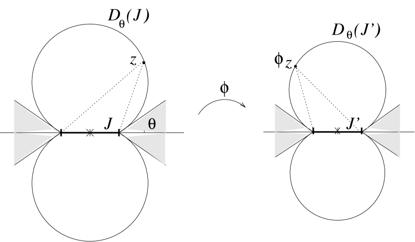
Figure 1.

Proof.

Let us normalize the situation in this way: $J=J^{\prime}=[0,1]$. Notice that the smallest (closed) geodesic neighborhood $\operatorname{cl}D_{\theta}(J)$ enclosing $z$ satisfies:
$\operatorname{diam}D_{\theta}(J)\leq C(\epsilon)\operatorname{dist}(z,J)$ (cf Fig. 1 ).

Indeed, if $\theta\geq\epsilon/2$ then $\operatorname{diam}D_{\theta}(J)\leq C(\epsilon)$, which is fine since $\operatorname{dist}(z,J)\geq 1$.
Otherwise the intervals $[0,z]$ and $[1,z]$ cut out sectors of angle size at least $\epsilon/2$ on the circle $\partial D_{\theta}(J)$. Hence the lengths of these intervals are commensurable with $\operatorname{diam}D_{\theta}(J)$ (with a constant depending on $\epsilon$). Also, by elementary trigonometry these lengths are at least $\sqrt{2}\operatorname{dist}(z,J)$, provided that $\operatorname{dist}(z,J)\geq|J|$.

By Schwarz Lemma, $\operatorname{dist}(\phi z,J^{\prime})\leq\operatorname{diam}(D_{\theta}(J^{\prime})),$ and the claim follows. ∎

2.3. Square root

In the next lemma we collect for future reference some elementary properties of the square root map. Let $\phi(z)=\sqrt{z}$ be the branch of the square root mapping the slit plane ${\mathbb{C}}\setminus{\mathbb{R}}_{-}$ into itself.

Lemma 2.2.

Let $K>1$, $\delta>0$, $K^{-1}\leq a\leq K$, $T=[-a,1]$, $T^{\prime}=[0,1]$. Then:

• $\phi D_{\theta}(T)\subset D_{\theta^{\prime}}(T^{\prime})$, with $\theta^{\prime}$ depending on $\theta$ and $K$ only.

• If $z^{\prime}\in\phi D(T)\setminus D([-\delta,1+\delta])$, then

  $$\widehat{(z^{\prime},T^{\prime})}>\epsilon(K,\delta)>0\quad and\quad C(K,\delta)^{-1}<\operatorname{dist}({z^{\prime}},{T^{\prime}})<C(K,\delta).$$

Lemma 2.3.

Let $\zeta\in\mathbb{C}$, $J=[a,b]\subset[0,+\infty)$. $\zeta^{\prime}=\phi(\zeta)$, $J^{\prime}=[a^{\prime},b^{\prime}]=\phi J$. Then:

• If $\operatorname{dist}(\zeta,J)>\delta|J|$ then

  $$\frac{\operatorname{dist}(J^{\prime},\zeta^{\prime})}{|J^{\prime}|}<C(\delta)\frac{\operatorname{dist}(J,\zeta)}{|J|}.$$

• Let $\theta$ denote the angle between $[\zeta,a]$ and the ray of the real line which does not contain $J$; $\eta^{\prime}$ denote the angle between $[\zeta^{\prime},b^{\prime}]$ and the corresponding ray of the real line. If $\theta\leq\pi/2$ then $\eta^{\prime}\geq\pi/4$.

(According to our convention, in the last statement we don’t assume that $a<b$.)

2.4. Branched coverings

Let $0\in U^{\prime}\subset U\subset{\mathbb{C}}$ be two topological disks different from the whole plane, and $f:U^{\prime}\rightarrow U$ be an analytic branched double covering map with critical point at 0. Thinking of it as a dynamical system, one can naturally define the filled Julia set $K(f)$ and the Julia set $J(f)$. Namely, the filled Julia set is the set of non-escaping points,

$$K(f)=\{z:f^{n}z\in U^{\prime},n=0,1,\ldots\},$$

and $J(f)=\partial K(f)$. These sets are not necessarily compact.

If additionally $\operatorname{cl}U^{\prime}\subset U$ then the map $f$ is called quadratic-like. The Julia set of a quadratic-like map is compact, and this is actually the criterion for being quadratic-like (for appropriate choice of domains):

Lemma 2.4 (compare [McM2], Proposition 4.10).

Let $U^{\prime}\subset U$ be two topological disks. and $f:U^{\prime}\rightarrow U$ be a double branched covering with non-escaping critical point and compact Julia set. Then there are topological discs $J(f)\subset V^{\prime}\subset V\subset U$ such that the restriction $g:V^{\prime}\rightarrow V$ is quadratic-like. Moreover, if $\mod(U\setminus K(f)\geq\epsilon>0$ then $\mod(V\setminus V^{\prime})\geq\delta(\epsilon)>0$.

Proof.

Let us consider the topological annulus $A=U\setminus K(g)$. Let $\phi:A\rightarrow R=\{z:1<|z|<r\}$ be its uniformization by a round annulus. It conjugates $g$ to a map $G:R^{\prime}\rightarrow R$ where $R^{\prime}$ is a subannulus of $R$ with the same inner boundary, unit circle $S^{1}$. As $G$ is proper near the unit circle, it is continuously extended to it, and then can be reflected to the symmetric annulus. We obtain the double covering map $\hat{G}:\hat{R}^{\prime}\rightarrow\hat{R}$ of the symmetric annuli preserving the circle. Moreover $\hat{R}$ is a round annulus of modulus at least $2\epsilon$.

Let $l$ denote the hyperbolic length on $\hat{R}$, $\hat{V}$ denote the hyperbolic 1-neighborhood of $S^{1}$, and $\hat{V}^{\prime}=\hat{G}^{-1}\hat{V}\subset\hat{V}$. As $\hat{G}:S^{1}\rightarrow S^{1}$ is a double covering, we have:

$$2l(S^{1})=\int_{S^{1}}\|Df(z)\|dl\leq\max_{S^{1}}\|Df(z)\|l(S^{1}),$$

so that $\max_{S^{1}}\|Df(z)\|\geq 2$. As $\mod\hat{R}\geq 2\epsilon$, $l(S^{1})\leq L(\epsilon)$. Hence $\|Df(z)\|\geq\rho(\epsilon)>1$ for all $z\in\hat{V}$. It follows that $\hat{V}^{\prime}$ is contained in $(1/\rho(\epsilon))$-neighborhood of $S^{1}$. But then each component of $V\setminus V^{\prime}$ is an annulus of modulus at least $\delta(\epsilon)>0$.

We obtain now the desired domains by going back to $U$: $V=\phi^{-1}\hat{V}$, $V^{\prime}=\phi^{-1}\hat{V}^{\prime}.$ ∎

Let us supply the space ${\cal B}$ of double branched maps considered above with the Caratheodory topology (see [McM1]). Convergence of a sequence $f_{n}:U_{n}^{\prime}\rightarrow U_{n}$ in this topology means Caratheodory convergence of $(U_{n},0)$ and $U_{n}^{\prime},0)$, and compact-open convergence of $f_{n}$.

2.5. Epstein class

A double branched map $f:U^{\prime}\rightarrow U$ of class ${\cal B}$ belongs to Epstein class if $U=\mathbb{C}_{T}$, $U^{\prime}$ is an $\mathbb{R}$-symmetric domain meeting the real line along an interval $T\supset T^{\prime}$, and the map $f$ is $\mathbb{R}$-symmetric. In this case its restriction $f:T^{\prime}\rightarrow T$ is a unimodal map. We always normalize $f$ in such a way that 0 is its critical point.

Given a $\lambda\in(0,1)$, let $\cal E_{\lambda}$ denote the space of maps of Epstein class with

$$\lambda|T^{\prime}|\leq|T|\leq\lambda^{-1}|T^{\prime}|,$$

modulo affine conjugacy (that is, rescaling of $T$).

Lemma 2.5.

For each $\lambda\in(0,1)$, the space $\cal E_{\lambda}$ is compact.

Proof.

Normality argument. ∎

All maps in this paper will be assumed to belong to some Epstein class.

2.6. Renormalization.

We assume that the reader is familiar with the notion of renormalization in one-dimensional dynamics (see e.g., [MS]).

Let $f$ be infinitely renormalizable. Let $P^{k}\ni 0$ be the central periodic interval corresponding to the $k$-fold renormalization $R^{k}f$ of $f$, $n_{k}$ be its period: $f_{k}\equiv R^{k}f\equiv f^{n_{k}}:P^{k}\rightarrow P^{k}$. Set $P_{m}^{k}=f^{m}P^{k}$. We say that the intervals $P^{k}_{i},\;i=0,1,\ldots,n_{k}-1,$ form the cycle of level $k$ .

Note that the periodic interval $P^{k}$ is not canonically defined. The maximal choice is $P^{k}=B^{k}=[\beta_{k},\beta_{k}^{\prime}]$ where $\beta_{k}$ is the fixed point of $f_{k}$ with positive multiplier. The minimal choice is $P^{k}=[f_{k}0,f_{k}^{2}0]$.

Let $p_{k}=n_{k}/n_{k-1}$ be relative periods. Combinatorics of $f$ is said to be bounded if the sequence of relative periods is bounded. Let $G^{k}_{l}$ be the gaps of level $k$, that is the components of $P^{k-1_{j}}\setminus\cup P^{k}_{i}$. Geometry of $f$ is said to be bounded if there is a $\Delta>0$ and a choice of periodic intervals $P^{k}_{i}$, such that for any $P_{i}^{k},G^{k}_{l}\subset P_{j}^{k-1},\;\;$ $|P_{i}^{k}|/|P^{k-1}_{j}|>\Delta$ and $|G^{k}_{l}|/|P^{k-1}_{j}\geq\Delta$. In other words, all intervals and gaps of level $k$ contained in some interval of level $k-1$ are commensurable with the latter.

Theorem A

Infinitely renormalizable maps with bounded combinatorics have bounded geometry.

For a proof the reader is referred to [G, BL1, BL2, S, MvS].

Let $S^{k}\supset P_{1}^{k}$ be the maximal symmetric interval around $0$ such that the restriction of $f_{k}$ to it is unimodal, and $T^{k}=f_{k}S^{k}$. Then $P^{k}\subset\ S^{k}\subset T^{k}$, and there is a definite space in between any two of these intervals. In the case of bounded (and essentially bounded) combinatorics all three intervals are commensurable. Moreover, if $f$ belongs to Epstein class, then the renormalizations $f_{k}$ are also maps of Epstein class, with range $\mathbb{C}_{T^{k}}$.

Corollary B

If $f$ is an infinitely renormalizable map of Epstein class with bounded combinatorics, then all renormalizations $R^{n}f$ belong to some Epstein class ${\cal E}_{\lambda}$. Hence the sequence $R^{n}f$ is pre-compact.

3. Outline of the proof

3.1. Main lemmas

Let $P^{k}$, $f_{k}\equiv R^{k}f\equiv f^{n_{k}}$ be as above.

Let us consider the decomposition:

(3.1) $$f_{k}=\psi_{k}\circ f,$$

where $\psi_{k}$ is a univalent map from a neighborhood of $P^{k}_{1}$ onto $\mathbb{C}_{T^{k}}$.

At §5 we will define the essential period $p_{e}(f)$. For the time being the reader can just replace this by the period $p(f)=n_{1}$.

Lemma 3.1.

Let $f$ be a $k$ times renormalizable quadratic map. Assume that $p_{e}(R^{l}f)\leq\bar{p}$ for $l=0,1,\ldots,k-1$. Then there exist constants $C,D$, depending on $\bar{p}$ only, such that $\forall z\in\mathbb{C}_{T^{k}}$ with $\operatorname{dist}(z,P^{k})\geq|P^{k}|$ the following estimate holds:

(3.2) $$\frac{\operatorname{dist}(\psi_{k}^{-1}z,P^{k}_{1})}{|P^{k}_{1}|}\leq C\left(\frac{\operatorname{dist}(z,P^{k})}{|P^{k}|}\right)+D,$$

where $\psi_{k}$ is the univalent map from 3.1

Thus the maps $\psi_{k}^{-1}$ have at most linear growth depending only on the combinatorial bound $\bar{p}$.

Note that if $\widehat{(z,P^{k})}>\epsilon>0$, the inequality 3.2 follows directly from Lemma 2.1, with the constants depending on $\epsilon$. Our strategy of proving Lemma 3.1 is to monitor the inverse orbit of a point $z$ together with the interval $P^{k}$ until they satisfy this ”good angle” condition.

Lemma 3.1 immediately yields the key quadratic estimate 1.1, which in turn implies:

Corollary 3.2.

The little Julia set $J(R^{k}f)$ is commensurable with the interval $P^{k}$.

Carrying the argument for Lemma 3.1 further, we will prove the following result:

Lemma 3.3.

Under the circumstances of the previous lemma, the little Julia set $J(R^{k}f)$ is contained in the hyperbolic disk $D_{\epsilon}(B^{k}),$ where $\epsilon>0$ depends only on $\bar{p}$.

3.2. Proof of the main results.

Proof of Theorem 1.1. It follows immediately from Lemma 3.3 and Lemma 2.4. $\sqcup$$\sqcap$

Proof of Corollary 1.2. By [L3], there is a $\bar{p}$ such that $\mod(Rf)\geq\mu>0$ for all renormalizable maps $f$ of Epstein class with $p_{e}(f)\geq\bar{p}$.

So given a quadratic polynomial, we have complex bounds for all renormalizations $R^{n+1}f$ such that $p_{e}(R^{n}f)\geq\bar{p}$. For all intermediate levels we have bounds by Theorem 1.1. $\sqcup$$\sqcap$

By a puzzle piece we mean a topological disk bounded by rational external rays and equipotentials (compare [H, L4, M1])

Proof of Corollary 1.3. By Corollary 3.2 the little Julia sets $J(f_{k})$ shrink to the critical point. By the Douady and Hubbard renormalization construction (see [D, L4, M2]), each little Julia set is the intersection of a nest of puzzle pieces. As each of these pieces contains a connected part of the Julia set, $J(f)$ is locally connected at the critical point.

Let us now prove local connectivity at any other point $z\in J(f)$ (by a standard ”spreading around” argument). Take a puzzle piece $V\ni 0$. The set of points which never visit $V$, $Y_{V}=\{\zeta:f^{n}\zeta\not\in V,\;n=0,1,\dots\}$, is expanding. (Cover this set by finitely many non-critical puzzle pieces, thicken them a bit, and use the fact the branches of the inverse map are contracting with respect to the Poincaré metric in these pieces). It follows that if $z\in Y_{V}$ then there is a nest of puzzle pieces shrinking to $z$, and we are done.

By Lemma 3.3, there is a nest of puzzle pieces $V^{k}\supset J(f_{k})$ contained in the Poincaré disk $D_{\theta}(B^{k})$, with $\theta>0$ depending only on $\bar{p}$. But because of bounded geometry (or, more generally, ”essentially bounded geometry”, see §5), there is a definite gap between the interval $B^{k}$ and the rest of the postcritical set $\omega(0)$. (That is, there is an $\epsilon=\epsilon(\bar{p})>0$ such that the interval $(1+\epsilon)B^{k}\setminus B^{k}$ does not intersect $\omega(0)$.) Thus the annuli $R^{k}=\mathbb{C}_{(1+\epsilon)B^{k}}\setminus D_{\theta}(B^{k})$ don’t meet the postcritical set. Moreover, all these annuli are similar and hence have the same moduli.

Assume now that $f^{l_{k}}z\in V^{k}$. Then there exist single-valued inverse branches $f^{-l_{k}}:\mathbb{C}_{(1+\epsilon)B^{k}}\rightarrow\mathbb{C}$ whose images contain $z$. By the Koebe theorem, they have a bounded distortion on puzzle pieces $V^{k}$. As $U^{k}=f^{-l_{k}}V^{k}$ cannot contain a disk of a definite radius, we conclude that $\operatorname{diam}U^{k}\to 0$. This is the desired nest of puzzle pieces about $z$. $\sqcup$$\sqcap$

Proof of Corollary 1.4. This result follows from Theorem D of [L3] and Theorem 1.1.$\sqcup$$\sqcap$

4. Bounded Combinatorics

We first show the existence of the complex bounds in the case when the map $f$ has bounded combinatorics. The result is well-known in this case [MvS, S], but we give a quite simple proof which will be then generalized for the case of essentially bounded combinatorics.

4.1. The $\epsilon$-jumping points

Given an interval $T\in\mathbb{R}$ let $f:U^{\prime}\rightarrow\mathbb{C}_{T}$ be a map of Epstein class.

For a point $x\in{\mathbb{R}}\cap U^{\prime}$ which is not critical for $f^{n}$, let $V_{n}(x)\equiv V_{n}(x,f)$ denote the maximal domain containing $x$ which is univalently mapped by $f^{n}$ onto $\mathbb{C}_{T}$. Its intersection with the real line is the monotonicity interval $H_{n}(x)\equiv H_{n}(x,f)$ of $f^{n}$ containing $x$. Let $f^{-n}_{x}:\mathbb{C}_{T}\rightarrow V_{n}(x)$ denote the corresponding inverse branch of $f^{-n}$ (continuous up to the boundary of the slits, with different values on the different banks). If $J$ is an interval on which $f^{n}$ is monotone, then the notations $V_{n}(J)$ and $H_{n}(J)$ and $f^{-n}_{J}$ make an obvious sense.

Take an $x\in\mathbb{R}$ and a $z\in\mathbb{C}_{T}$. If we have a backward orbit of $x\equiv x_{0},x_{-1},\dots,x_{-l}$ of $x$ which does not contain 0, the corresponding backward orbit $z\equiv z_{0},z_{-1},\dots,z_{-l}$ is obtained by applying the appropriate branches of the inverse functions: $z_{-n}=f_{x_{-n}}z$. The same terminology is applied when we have a monotone pullback $J\equiv J_{0},\dots,J_{-l}$ of an interval $J$.

Let $H\supset J$ be two intervals. Let $S_{\theta,\epsilon}(H,J)$ denote the union of two $2\epsilon$-wedges with vertices at $\partial J$ (symmetric with respect to the real line) cut off by the neighborhood $D_{\theta}(H)$ (cf. Fig. 2).

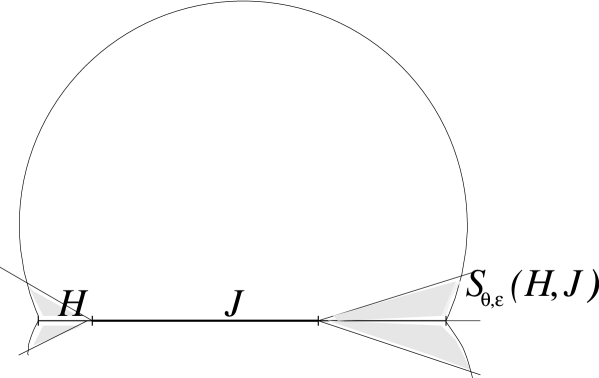
Figure 2.

Let $Q_{\epsilon}(J)$ denote the complement of the above two wedges (that is, the set of points looking at $J$ at an angle at least $\epsilon$).

Lemma 4.1.

Let $f$ be a quadratic map. Let $J\equiv J_{0},J_{-1},\dots,J_{-l}\equiv J^{\prime}$ be a monotone pullback of an interval $J$, $z\equiv z_{0},z_{-1},\ldots,z_{-l}\equiv z^{\prime}$ be the corresponding backward orbit of a point $z\in\mathbb{C}_{T}$. Then for all sufficiently small $\epsilon>0$ (independent of $f$), either $z_{-k}\in Q_{\epsilon}(J_{-k})$ at some moment $k\leq l$, or $z^{\prime}\in S_{\theta,\epsilon}(H_{l}(J^{\prime}),J^{\prime})$ with $\theta=\pi/2-0(\epsilon)$.

If the first possibility of the lemma occurs we say that the backward orbit of $z$ ”$\epsilon$-jumps”.

Proof.

Assume that the backward orbit of $z$ does not “$\epsilon$-jump”, that is, $z_{-k}$ belongs to an $\mathbb{R}$-symmetric $2\epsilon$-wedge centered at $a_{-k}\in\partial J_{-k}$, $k=0,1\ldots,l$. By the second statement of Lemma 2.3, $fa_{-(k+1)}=a_{-k}$. Let $M_{-k}=f^{l-k}H_{n}(J^{\prime})$, and $b_{-k}$ be the boundary point of $M_{k}$ on the same side of $J_{-k}$ as $a_{-k}$. Let us take the moment $k$ when $b_{-k}=0$. At this moment the point $z_{-k}$ belongs to a right triangle based upon $[a_{-k},b_{-k}]$ with the $\epsilon$-angle at $a_{-k}$ and the right angle at $b_{-k}$. Hence $z_{-k}\in D_{\theta}(M_{-k})$ with $\theta=\pi/2-0(\epsilon)$. It follows by Schwarz Lemma that $z^{\prime}\in D_{\theta}(H_{l}(J^{\prime}),J^{\prime})$, and we are done. ∎

Let us state for the further reference in §7 a straightforward extension of the above lemma onto maps of Epstein class:

Lemma 4.2.

The conclusion of Lemma 4.1 still holds for all $\epsilon<\epsilon(\lambda)$, provided $f:U^{\prime}\rightarrow\mathbb{C}_{T}$ is a map of Epstein class $\cal E_{\lambda}$, $U^{\prime}\subset\mathbb{C}_{\lambda T}$, and $z\in D(\lambda T)$.

4.2. Proof of Lemma 3.1 (for bounded combinatorics).

For technical reasons we consider a new family of intervals $\tilde{S}^{k}$ and $\tilde{T}^{k}$, for which $P^{k}\subset\tilde{S}^{k}\subset S^{k}\subset\tilde{T}^{k}\subset T^{k}$, each of the intervals is commensurable with the others and contained well inside the next one, and $f_{k}(\tilde{S}^{k})=\tilde{T}^{k}$.

Let us fix a level $k$, and set $n\equiv n_{k}$,

(4.1) $$J_{0}\equiv P^{k}_{0},J_{-1}\equiv P^{k}_{n-1},\ldots,J_{-(n-1)}\equiv P^{k}_{1}.$$

Take now any point $z_{0}\in\mathbb{C}_{T^{k}}$ with $\operatorname{dist}(z_{0},J_{0})\geq|J_{0}|$, and let $z_{-1},\ldots,z_{-(n-1)}$ be its backward orbit corresponding to the above backward orbit of $J_{0}$. Our goal is to prove that

(4.2) $${\operatorname{dist}(z_{-(n-1)},J_{-(n-1)})\over|J_{-(n-1)}|}\leq C(\bar{p}){\operatorname{dist}(z_{0},J_{0})\over|J_{0}|}.$$

Take a big quantifier $\bar{K}>0.$ Let is say that $s$ is a ”good” moment of time if $J_{-s}$ is $\bar{K}$-commensurable with $J_{0}$. For example, let $J_{-s}\subset P^{l}$ and $s\leq n_{l+1}$. In other words, $s$ is a moment of backward return to $P^{l}$ preceding the first return to $P^{l+1}$. By bounded geometry, this moment is good, provided $\bar{K}$ is selected sufficiently big.

Let us first consider the initial piece of the orbit, $z_{0},\ldots,z_{-n_{1}},$ corresponding to the renormalization cycle of level $1$. By the first statement of Lemma 2.3, for all $s\in[0,n_{1}-1]$,

(4.3) $${\operatorname{dist}(z_{-s},J_{-s})\over|J_{-s}|}\leq C_{0}(\bar{p}){\operatorname{dist}(z_{0},J_{0})\over|J_{0}|}.$$

By Lemma 4.1, either

(4.4) $$z_{-n_{1}}\in D(S^{1})\subset D(\tilde{T}^{1}),$$

or there is a moment $-s\in[-n_{1},0]$ when the backward orbit $\epsilon$-jumps: $\widehat{(z_{-s},J_{-s})}>\epsilon$. In the latter case the desired estimate (4.2) follows from (4.3) and Lemma 2.1. In the former case we will proceed inductively:

Lemma 4.3.

Let $J=J_{-s}$ and $J^{\prime}=J_{-(s+n_{l})}$ be two consecutive returns of the backward orbit (4.1) to a periodic interval $P^{l}$, $l<k$. Let $z$ and $z^{\prime}$ be the corresponding points of the backward orbit of $z_{0}$. If $z\in D(\tilde{T}^{l})$ then $\operatorname{dist}(z^{\prime},J^{\prime})\leq C(\bar{p})|\tilde{T}^{l}|$. Moreover, either $z^{\prime}\in D(\tilde{T}^{l})$, or $\widehat{(z^{\prime},J^{\prime})}>\epsilon(\bar{p})>0$.

Proof.

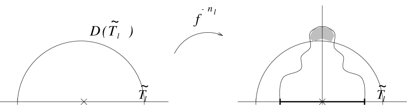
Figure 3.

Let us consider decomposition (3.1). The diffeomorphism $\psi_{l}$ maps some interval $Z^{l}\supset fS^{l}$ onto $T^{l}$. Hence $\psi_{l}^{-1}$ has a bounded distortion on $\tilde{T}^{l}$. Let $\tilde{Z}^{l}=\psi_{l}^{-1}\tilde{T}^{l}\subset Z^{l}$.

By bounded geometry, the point $f_{l}0$ divides $\tilde{T}^{l}$ into commensurable parts. Hence the critical value $f0=\psi_{l}^{-1}(f_{l}0)$ divides $\tilde{Z}^{l}$ into commensurable parts: Let $A=A(\bar{p})$ stand for a bound of the ration of these parts.

By the Schwarz lemma, domain $V=\psi_{l}^{-1}(D(\tilde{T}^{l}))$ is contained in $D(\tilde{Z}^{l})$. Hence its pullback $f^{-1}V$ by the quadratic map is contained in a domain $W=f^{-1}D(\tilde{Z}^{l})$ intersecting the real line by $\tilde{S}^{l}$, and having a bounded distortion about 0. Hence $\operatorname{diam}W\leq C(\bar{p})\tilde{S}^{l}$, which proves the first statement.

Finally, it follows from Lemma 2.2, that $W\setminus D(\tilde{T}^{l})$ is contained in a sector $Q_{\epsilon}(\tilde{S}^{l})$ with an $\epsilon$ depending only on $A=A(\bar{p})$ (see Figure 3).

∎

Let us now give a more precise statement:

Lemma 4.4.

Let $J=J_{-s}$ and $J^{\prime}=J_{-s^{\prime}}$ be two returns of the backward orbit (4.1) to $P^{l}$, where $s^{\prime}=s+tn_{l}$. Let $z$ and $z^{\prime}$ be the corresponding points of the backward orbit of $z_{0}$. Assume $z\in D(\tilde{T}^{l})$. Then either for some $0\leq i\leq t$, a point $z_{-(s+in_{l})}$ $\epsilon$-jumps and $|z_{-(s+in_{l})}|\leq C|T^{l}|$, or $z_{-s^{\prime}}\in D_{\theta^{\prime}}(H^{\prime})$, where $H^{\prime}$ is the monotonicity interval of $f^{tn_{l}}$ containing $J^{\prime}$, and $\theta^{\prime}=\pi/2-O(\epsilon)$.

Proof.

Assume that the above points do not $\epsilon$-jump. Then by Lemma 4.3 they belong to the disk $D(\tilde{T}^{l})$. As the map $\psi_{l}^{-1}$ from 3.1 has a bounded distortion, non of the points $z_{-m}$ $\delta$-jumps for $s\leq m\leq s^{\prime}$, where $\delta=O(\epsilon)$ as $\epsilon\to 0$. Now the claim follows from Lemma 4.1. ∎

The following lemma will allow us to make an inductive step:

Corollary 4.5.

Let $J=J_{-(n_{l})}$, $J^{\prime}=J_{-n_{l+1}}$, and $z,z^{\prime}$ be the corresponding points of the backward orbit of $z_{0}$. Assume $z\in D(\tilde{T}^{l-1})$. Then either there is a good moment $-m\in(-n_{l},-n_{l+1})$ when the point $z_{-m}$ $\epsilon$-jumps and $|z_{-m}|\leq C|T^{l}|$, or $z^{\prime}\in D(\tilde{T}^{l})$.

Proof.

Note that by bounded geometry all the moments

$$-n_{l},-(n_{l}+n_{l-1}),-(n_{l}+2n_{l-1}),\ldots,-n_{l+1},$$

when the intervals of (4.1) return to $P^{l-1}$ before the first return to $P^{l+1}$, are good (provided the quantifier $\bar{K}$ is selected sufficiently big). Hence by Lemma 4.4 either the first possibility of the claim occurs, or $z^{\prime}\in D_{\theta^{\prime}}(L^{\prime})$, where $L^{\prime}$ is the monotonicity interval of $f^{n_{l+1}-n_{l}}$ containing $J^{\prime}$, and $\theta^{\prime}=\pi/2-O(\epsilon)$. As $n_{l+1}-n_{l}\geq n_{l}$, $L^{\prime}$ is contained in $S^{l}$, which is well inside $\tilde{T}^{l}$. Thus $D_{\theta^{\prime}}(L^{\prime})\subset D(\tilde{T}^{l}),$ provided $\epsilon$ is sufficiently small. ∎

We are ready to carry out the inductive proof of (4.2). Set $j=0$ if $z_{0}\not\in D(\tilde{T}^{0})$. Otherwise let $j$ be the smallest level for which

(4.5) $$z_{0}\in D(\tilde{T}^{j}).$$

By the considerations in the beginning of the proof (if $j=0$) or by Lemma 4.3 (for $j>0$), either $z_{-n_{j}}\in D(\tilde{T}^{j})$, or $z_{-n_{j}}$ $\epsilon$-jumps. Moreover, in the latter case $|z_{-n_{j}}|\leq C|z_{0}|$, so that (4.2) follows.

In the former case we will proceed inductively. Assume that either $z_{-n_{l}}\in D(\tilde{T}^{l-1})$, or $z_{-t}$ $\epsilon$-jumps at some good moment $-t\geq s$. If the latter happens, we are done. If the former happens, we pass to $l+1$ by Corollary 4.5. Lemma 3.1 is proven.

4.3. Proof of Lemma 3.3 (for bounded combinatorics)

By Corollary 3.2, $\operatorname{diam}J(f_{k})\leq C|T^{k}|,$ with a $C=C(\bar{p})$. Hence $J(f_{k})\subset D(\tilde{T}^{l})$, where $l\geq k-N(\bar{p})$. Let $\zeta^{\prime}\in J(f_{k})$, $\zeta=f_{k}\zeta^{\prime}$, and $\zeta=\zeta_{0},\zeta_{-1},\ldots,\zeta_{-n}=\zeta^{\prime}$ be the corresponding backward orbit under iterates of $f_{l}$.

By Lemma 4.3, either $\zeta_{-j}$ $\epsilon$-jumps at some moment, or $\zeta^{\prime}\in D(\tilde{T}^{k})$. If the former happens then $\zeta_{-j}\in D_{\theta}(J_{-jn_{l}})$, where $\theta=\theta(\epsilon)>0,$ and $J_{-m}$ are the intervals from 4.1. But then by the Schwarz Lemma $\zeta^{\prime}\in D_{\theta^{\prime}}(P^{k})$ with some $\theta^{\prime}$ depending on $\bar{p}$ only. Thus $J(f_{k})\subset D_{\theta^{\prime}}(P^{k})\cup D(\tilde{T}^{k}),$ and we are done.

Remark 4.1.

The above proof of the main lemmas for the case of bounded combinatorics illustrates the ideas involved in treating the general essentially bounded case. A complication arises however because of the possibility that a jump in the orbit occurs at a ”bad” moment when the corresponding iterate of the periodic interval is not commensurable with its original size.

5. Essentially Bounded Combinatorics and Geometry

Let $f$ be a renormalizable quasi-quadratic map.

We use the standard notations $\beta$ and $\alpha$ for the fixed points of $f$ with positive and negative multipliers correspondingly. Let $B\equiv B(f)=[\beta,\beta^{\prime}]$, $A\equiv A(f)=[\alpha,\alpha^{\prime}]\subset B$.

The map $f$ is called immediately renormalizable if the interval $A$ is periodic with period $2$. If $f$ is not immediately renormalizable, let us consider the principal nest $A\equiv I^{0}\equiv I^{0}(f)\supset I^{1}\equiv I^{1}(f)\supset\dots$ of intervals of $f$ (see [L2]). It is defined in the following way. Let $t(m)$ be the first return time of the orbit of 0 back to $I^{m-1}$. Then $I^{m}$ is defined as the component of $f^{-t(m)}I^{m-1}$ containing 0. Moreover $\cap_{m}I^{m}=B(Rf)$.

For $m>1$, let

$$g_{m}:\bigcup_{i}I^{m}_{i}\rightarrow I^{m-1}$$

be the generalized renormalization of $f$ on the interval $I^{m-1}$, that is, the first return map restricted onto the intervals intersecting the postcritical set (here $I^{m}\equiv I^{m}_{0}$). Note that $g_{m}\equiv f^{t(m)}:I^{m}\rightarrow I^{m-1}$ is unimodal with $g_{m}(\partial I^{m})\subset\partial I^{m-1}$, while $g_{m}:I^{m}_{i}\rightarrow I^{m-1}$ is a diffeomorphism for all $i\not=0$.

Let us consider the following set of levels:

$$X\equiv X(f)=\{m:t(m)>t(m-1)\}\cup\{0\}=\{m(0)<m(1)<m(2)<\dots<m(\chi)\}.$$

A level $m=m(k)$ belongs to $X$ iff the return to level $m-1$ is non-central, that is $g_{m}0\in I^{m-1}\backslash I^{m}$. For such a moment the map $g_{m+1}$ is essentially different from $g_{m}$ (that is not just the restriction of $g_{m}$ to a smaller domain). Let us use the notation $h_{k}\equiv g_{m(k)+1}$, $k=1,\ldots\chi$. The number $\chi=\chi(f)$ is called the height of $f$ ( In the immediately renormalizable case set $\chi=-1$).

The nest of intervals

(5.1) $$I^{m(k)+1}\supset I^{m(k)+2}\supset\ldots\supset I^{m(k+1)}$$

is called a central cascade. The length $l_{k}$ of the cascade is defined as $m(k+1)-m(k)$. Note that a cascade of length 1 corresponds to a non-central return to level $m(k)$.

A cascade 5.1 is called saddle-node if $h_{k}I^{m(k)+1}\not\ni 0$ (see Fig. 4). Otherwise it is called Ulam-Neumann. For a long saddle-node cascade the map $h_{k}$ is combinatorially close to $z\mapsto z^{2}+1/4$. For a long Ulam-Neumann cascade it is close to $z\mapsto z^{2}-2$.

Figure 4. A long saddle-node cascade

Given a cascade (5.1), let

(5.2) $$K_{j}^{m(k)+i}\subset I^{m(k)+i-1}\setminus I^{m(k)+i},\;i=1,\dots,m(k+1)-m(k)-1$$

denote the pull-back of $I_{j}^{m(k)+1}$ under $h_{k}^{i-1}=g^{i-1}_{m(k)+1}$. Clearly, $K_{j}^{m(k)+i+1}$ are mapped by $h_{k}$ onto $K_{j}^{m(k)+i}$, $i=1,\dots,m(k+1)-m(k)-1$, while $K_{j}^{m(k)+1}\equiv I_{j}^{m(k)+1}$ are mapped onto the whole $I^{m(k)}$. This family of intervals is called the Markov family associated with the central cascade.

Let $x\in\omega(0)\cap(I^{m(k)}\setminus I^{m(k)+1})$, $h_{k}x\in I^{j}\setminus I^{j+1}$. Set

$$d(x)=\min\{j-m(k),m(k+1)-j\}.$$

This parameter shows how deep the orbit of $x$ lands inside the cascade. Let us now define $d_{k}$ as the maximum of $d(x)$ over all $x\in\omega(0)\cap(I^{m(k)}\setminus I^{m(k)+1})$.

Given a saddle-node cascade (5.1), let us call all levels $m(k)+d_{k}<l<m(k+1)-d_{k}$ neglectable.

Let us now define the essential period $p_{e}=p_{e}(f)$. Let $p$ be the period of the periodic interval $J=B(Rf)$. Let us remove from the orbit $\{f^{k}J\}_{k=0}^{p-1}$ all intervals whose first return to some $I^{m(k)}$ belongs to a neglectable level. The essential period is the number of the intervals which are left.

We say that an infinitely renormalizable map $f$ has essentially bounded combinatorics if $\sup_{n}p_{e}(R^{n}f)<\infty$.

Let $\sigma(f)=|B(Rf)|/|B(f)|$. Let us say that $f$ has essentially bounded geometry if $\inf_{n}\sigma(R^{n})>0$.

Theorem 5.1.

[L3, Theorem D] Let $f$ be a quasi-quadratic map of Epstein class. There are functions $\delta(p)\geq\epsilon(p)>0$, such that $\delta(p)\to 0$ as $p\to\infty$, with the following properties. If $p_{e}(f)\leq p$ then $\sigma(f)\geq\epsilon(p)$. Vice versa, if $p_{e}(f)\geq p$ then $\sigma(f)\leq\delta(p)$. Thus geometry of $f$ is essentially bounded if and only if its combinatorics is.

From now on we will work only with maps having essentially bounded combinatorics, and $\bar{p}$ will stand for a bound of the essential period. By the gaps $G^{m}_{j}$ of level $m$ we mean the components of $I^{m-1}\setminus\cup I^{m}_{j}$. We say that a level $m$ is deep inside the cascade if $m(k)+\bar{p}\leq m\leq m(k+1)-\bar{p}$. Let us finish this section with a lemma on geometry of maps with essentially bounded combinatorics.

Lemma 5.2.

[L3, Lemma 17] Let $f$ be a quasi-quadratic map with essentially bounded combinatorics. Then for any $m$, the non-central intervals $I^{m}_{i},\;i\not=0,$ and the gaps $G^{m}_{j}$ of level $m$ are $C(\bar{p})$-commensurable with $I^{m-1}\setminus I^{m}$. Moreover, this is also true for the central interval $I^{m}_{0}$, provided $m$ is not deep inside the cascade.

Note that the last statement of the lemma is definitely false when $m$ is deep inside the cascade: then $I^{m}$ occupies almost the whole of $I^{m-1}$. So we observe commensurable intervals in the beginning and in the end of the cascade, but not in the middle. This is the saddle-node phenomenon which is in the focus of this work.

6. Saddle-Node Cascades

Let $f\in\cal E_{\lambda}$ be a map of Epstein class.

Let us note first for a long saddle-node cascade 5.1, the map $h_{k}:I^{m(k)+1}\rightarrow I^{m(k)}$ is a small perturbation of a map with a parabolic fixed point.

Lemma 6.1.

[L3] Let $h_{k}$ be a sequence of maps of Epstein class $\cal E_{\lambda}$ having saddle-node cascades of length $l_{k}\to\infty$. Then any limit point $f:I^{\prime}\rightarrow I$ of this sequense (in the Caratheodory topology) has on the real line topological type of $z\mapsto z^{2}+1/4$, and thus has a parabolic fixed point.

Proof.

It takes $l_{k}$ iterates for the critical point to escape $I^{m(k)+1}$ under iterates of $h_{k}$. Hence the critical point does not escape $I^{\prime}$ under iterates of $f$. By the kneeding theory [MT] $f$ has on the real line topological type of $z^{2}+c$ with $-2\leq c\leq 1/4$. Since small perturbations of $f$ have escaping critical point, the choice for $c$ boils down to only two boundary parameter values, $1/4$ and $-2$. Since the cascades of $h_{k}$ are of saddle-node type, $fI^{\prime}\not\ni 0$, which rules out $c=-2$.

∎

Remark 6.1.

Thus the plane dynamics of $h_{k}$ with a long saddle node cascade resembles the dynamics of a map with a parabolic fixed point: the orbits follow horocycles (cf. Fig. 5).

Figure 5. The backward trajectory of a point corresponding to a saddle-node cascade

Lemma 6.2.

Let us consider a saddle-node cascade 5.1 generated by a return map $h_{k}$. Let us aslo consider a backward orbit of an interval $E\subset I^{m(k)}\setminus I^{m(k)+1}$ under iterates of $h_{k}$:

$$E\equiv E_{0},\;E_{-1}\subset I^{m(k)+1}\setminus I^{m(k)+2},\dots,E_{-j}\equiv E^{\prime}\subset I^{m(k)+j}\setminus I^{m(k)+j+1},$$

where $m(k)+j+i\leq m(k+1)$. Let $z=z_{0},z_{-1},z_{-2},\dots,z_{-j}=z^{\prime}$ be the corresponding backward orbit of a point $z\in D(I^{m(k)})$. If the length of the cascade is sufficiently big, then either $z^{\prime}\in D(I^{m(k)})$, or $\widehat{(z^{\prime},J^{\prime})}>\epsilon$ and $\operatorname{dist}(z^{\prime},J^{\prime})\leq C(\bar{p})|I^{m(k)}|$.

Proof.

To be definite, let us assume that the intervals $E_{-i}$ lie on the left of 0 (see Figure 4). Without loss of generality, we can assume that $z\in\mathbb{H}$. Let $\phi=h_{k}^{-1}$ be the inverse branch of $h_{k}$ for which $\phi E_{-i}=E_{-(i+1)}$. As $\phi$ is orientation preserving on $(-\infty,h_{k}0]$, it maps the upper half-plane $\mathbb{H}$ into itself: $\phi(\mathbb{H})\subset\{z=r^{ei\theta}|\;r>0,\;\pi>\theta>\pi/2\}$.

By Lemma 6.1, if the cascade 5.1 is sufficiently long, the map $\phi$ has an attracting fixed point $\eta_{\phi}\in\mathbb{H}\cap D(I^{m(k)+2})$ (which is a perturbation of the parabolic point for some map of type $z^{2}+1/4$). By the Denjoy-Wolf Theorem, $\phi^{n}(\zeta)\underset{n\rightarrow\infty}{\longrightarrow}\eta_{\phi}$ for any $\zeta\in\mathbb{H}$, uniformly on compact subsets of $\mathbb{H}$. Thus for a given compact set $K\Subset\mathbb{H}$, there exists $N=N(K,\phi)$ such that $\phi^{N}(K)\subset D(I^{m(k)+1})$. By a normality argument, the choice of $N$ is actually independent of a particular $\phi$ under consideration.

Suppose $z_{-r}\notin D(I^{m(k)})$. By Lemma 2.2 the set $K=D(I^{m(k)})\setminus\phi(D(I^{m(k)}))\cap\mathbb{H}$ is compactly contained in $\mathbb{H}$, and $\operatorname{diam}K\leq C|I^{m(k)}|$. For $N$ as above we have $z^{\prime}\in\cup_{i=0}^{N-1}\phi^{i}(K)\cup D(I^{m(k)})$ and the lemma is proved.

∎

7. Proofs of the Main Lemmas

7.1. Proof of Lemma 3.1

Let us start with a little lemma:

Lemma 7.1.

Let $f\in\cal E_{\lambda}$ be a map of Epstein class without attracting fixed points. Then both components of $B\setminus A$ contain an $f$-preimage of $0$ which divides them into $C(\lambda)$-commensurable parts.

Proof.

The interval $[\alpha,\beta^{\prime}]$ is mapped by $f$ onto $[\beta,\alpha]\ni 0$. Denote by $\eta=f^{-1}(0)\cap[\alpha,\beta^{\prime}]$. Under our assumption this point is clearly different from $\alpha$ and $\beta^{\prime}$. As the space of maps of Epstein class $\cal E_{\lambda}$ with no attracting fixed points is compact, $\eta$ divides $[\alpha,\beta^{\prime}]$ into $C(\lambda)$-commensurable parts. The analogous statement is certainly true for the symmetric point $\eta^{\prime}\in[\beta,\alpha^{\prime}]$. ∎

As in §4, let us fix a level $\tau$, let $n=n_{\tau}$, and set

(7.1) $$J_{0}\equiv P^{\tau},J_{1}\equiv P^{\tau}_{n-1},\dots,J_{-(n-1)}\equiv P^{\tau}_{1}.$$

For any point $z\in\mathbb{C}_{T^{\tau}}$ with $\operatorname{dist}(z,J_{0})>|J_{0}|$, we denote by

(7.2) $$z\equiv z_{0},z_{-1},z_{-2},\dots,z_{-(n-1)}$$

the backward orbit of $z$ corresponding to the orbit (7.1). We should prove that

(7.3) $${\operatorname{dist}(z_{-(n-1)},J_{-(n-1)})\over|J_{-(n-1)}|}\leq C(\bar{p}){\operatorname{dist}(z_{0},J_{0})\over|J_{0}|}.$$

Let $A=A(f)$ and $B=B(f)$ be the intervals defined in §5, $H_{s}(x)$ be the monotonicity intervals as defined in §4.1.

Lemma 7.2 (First return to $A$).

Let $J_{-s}$ be the first return of the orbit (7.1) to the interval $A$. There is an $\epsilon=\epsilon(\bar{p})>0$ such that either $z_{-s}\in D(B),$ or there is a moment $-i\in[-s,0]$ when the backward orbit (7.2) $\epsilon$-jumps: $\widehat{(z_{-i},J_{-i})}>\epsilon$ and moreover

(7.4) $${\operatorname{dist}(z_{-i},J_{-i})\over|J_{-i}|}\leq C_{0}(\bar{p}){\operatorname{dist}(z_{0},J_{0})\over|J_{0}|}.$$

Proof.

By definition of the essential period, $s\leq p_{e}(f)\leq\bar{p}$. Hence (7.4) holds for all $i=0,1,\ldots,s$ by the first statement of Lemma 2.3.

Further, by Lemma 7.1 each component of $B\setminus A$ contains a preimage of $0$, and it divides $B$ into $K(\bar{p})$-commensurable intervals. Hence, the monotonicity interval $H=H_{s}(J_{-s})$ is well inside of $B$, and the conclusion follows from Lemma 4.1. ∎

If the second possibility of Lemma 7.2 occurs then (7.3) follows from Lemma 2.1. If the first one happens, we proceed inductively along the principal nest. Namely, in the following series of lemmas we will show that the backward $z$-orbit (7.2) either $\epsilon$-jumps at some good moment, or follows the backward $J$-orbit (7.1) with at most one level delay.

In the following lemmas we work with a fixed renormalization level $l$ and skip index $l$ in the notations: $f\equiv f_{l}\equiv R^{l}(f_{0})$, $A\equiv A^{l},B\equiv B^{l}$. We will use notations of §5 for different combinatorial objects.

Lemma 7.3 (Further returns to $A$).

Let $E=E_{0},E_{-1},\dots,E_{-s}=E^{\prime}$ be the consecutive returns of the backward orbit (7.1) to $B$, between two consecutive returns to $A$. Let $\zeta=\zeta_{0},\zeta_{-1},\dots\zeta_{-s}=\zeta^{\prime}$ be the corresponding points of the backward orbit (7.2). Assume $\zeta\in D(B)$. Then either $\zeta^{\prime}\in D(B)$, or $\widehat{(\zeta_{-i},E_{-i})}>\epsilon(\bar{p})>0$ and $\operatorname{dist}(\zeta_{-i},E_{-i})\leq C(\bar{p})|B|$ for some $0\leq i\leq s$.

Proof.

Take an $\epsilon>0$. By definition of the essential period, $s\leq\bar{p}$. By the Schwarz lemma and Lemma 2.2, $\zeta_{-i}\in D_{\sigma}(B)$ for $i=0,1\dots s$, with $\sigma=\sigma(\bar{p})$. Hence $\operatorname{dist}(\zeta_{-i},E_{-i})\leq C(\bar{p})|B|.$ If for some $i\in[0,s]$, $\widehat{(\zeta_{-i},E_{-i})}>\epsilon,$ we are done.

By Lemma 7.1 each component of $B\setminus A$ contains an $f$-preimage of 0 which divides $B$ into $K$-commensurable intervals, with $K=K(\bar{p})$. Hence the monotonicity interval of $f$, $H=H_{s}(E_{-s})$, is well inside of $B$. As $f:B\rightarrow B$ has an extension of Epstein class $\cal E_{\lambda}$ (see §2.6), we can apply Lemma 4.2. It follows that if none of the points $\zeta_{-i}$ $\epsilon$-jumps, then $\zeta_{-i}\in D_{\theta}(H)$, $0\geq-i\geq-s$, with $\theta=\pi/2-O(\epsilon)$. Thus $\zeta_{-s}\in D(B)$ for sufficiently small $\epsilon<\epsilon(\bar{p})$, and the proof is completed. ∎

We say that a point/interval is deep inside of the cascade (5.1) if it belongs to $I^{m(k)+\bar{p}}\backslash I^{m(k+1)-\bar{p}}$. (In the case of essentially bounded combinatorics such a cascade must be of saddle node type). Recall that a moment $-i$ is called “good” if the interval $J_{-i}$ is commensurable with $J_{0}$. Because of the essentially bounded geometry, this happens, e.g., when for some $k$, the interval $J_{-i}$ lies in $I^{m(k)}\setminus I^{m(k+1)}$ but is not deep inside the corresponding cascade.

Lemma 7.4 (First return to $I^{m(1)}$).

Assume that $f$ is not immediately renormalizable. Let $E\equiv E_{0},E_{-1},\dots,$ $E_{-s}\equiv E^{\prime}$ be the consecutive returns of the backward orbit (7.1) to $A$ until the first return to $I^{m(1)}$. Let $\zeta\in\mathbb{C}_{A}\cap D(B)$, and let $\zeta\equiv\zeta_{0},\zeta_{-1}\dots\zeta_{-s}\equiv\zeta^{\prime}$ be the corresponding points in the backward orbit of $\zeta_{0}$. Then either $\zeta^{\prime}\in D(A)$, or $\widehat{(\zeta_{-i},E_{-i})}>\epsilon(\bar{p})>0$ and $\operatorname{dist}(\zeta_{-i},E_{-i})\leq C(\bar{p})|B|$ at some good moment $0\geq-i\geq-s$.

Proof.

Let $H=H_{s}(E_{-s})$.

As $f$ is not immediately renormalizable, we have the interval $I^{1}=[p,p^{\prime}]$. Let $p$ be chosen on the same side of $0$ as $\alpha$. Then $f^{2}[\alpha,p]\supset[\alpha,\alpha^{\prime}]$. Denote by $\eta$ the $f^{2}$-preimage of $0$ in $[\alpha,p]$. Since $f$ is quadratic up to bounded distortion, the map $f^{2}|_{[\alpha,p]}$ is quasi-symmetric (that is, maps commensurable adjacent intervals onto commensurable ones). It follows that $\eta$ divides $[\alpha,p]$, and hence $A$, into $K=K(\bar{p})$-commensurable parts. Hence $H\subset[\eta,\eta^{\prime}]$ is well inside $A$.

By Lemma 4.2 and Lemma 7.3, either $\zeta^{\prime}\in D_{\theta}(H)$ with $\theta=\pi/2-O(\epsilon)$, or there is a moment $i\leq s$ such that

(7.5) $$\widehat{(\zeta_{-i},E_{-i})}>\epsilon\quad{\rm and}\quad\operatorname{dist}(\zeta_{-i},E_{-i})\leq C(\bar{p})|B|.$$

In the former case we are done as $D_{\theta}(H)\subset D(A)$ for sufficiently small $\epsilon$.

Let the latter case occur. Then we are done if the moment $-i$ is good. Otherwise $E_{-i}$ is deep inside the cascade $A=I^{0}\supset I^{1}\supset\dots\supset I^{m(1)}$. Consider the largest $r$ such that $E_{-(i+q)}\subset I^{t+q-1}\setminus I^{t+q}$ for all $0\leq q\leq r$. Note that by essentially bounded combinatorics, the moment $-j=-(i+r)$ has to be good. By Lemma 6.2, either (7.5) occurs for $\zeta_{-j}$, and we are done, or $\zeta_{-j}\in D(A)$.

In the latter case let $\tilde{K}\subset I^{m(1)-1}\setminus I^{m(1)}$ be the interval containing $E_{-(s-1)}$ which is homeomorphically mapped under $h_{1}^{s-1-j}$ onto $A$ (to see that such an interval exists, consider the Markov scheme described in §5). By the Schwarz lemma $\zeta_{-(s-1)}\in D(\tilde{K})\subset D(A)$. Now the claim follows from Lemma 2.2. ∎

Now we are in a position to proceed inductively along the principal nest: Note that the assumption of the following lemma is checked for $k=1$ in Lemma 7.4.

Lemma 7.5 (Further returns to $I^{m(k)}$).

Let $E$ and $E^{\prime}$ be two consecutive returns of the backward orbit (7.1) to the interval $I^{m(k)}$. Let $\zeta$ and $\zeta^{\prime}$ be the corresponding points of the backward orbit of $z_{0}$. Assume that $\zeta\in D(I^{m(k-1)})$. Then, either $\zeta^{\prime}\in D(I^{m(k)})$, or $\widehat{(\zeta^{\prime},E^{\prime})}>\epsilon(\bar{p})>0$, and $\operatorname{dist}(\zeta^{\prime},E^{\prime})<C(\bar{p})|I^{m(k-1)}|.$

Proof.

Denote by $\tilde{E}$ the last interval in the backward orbit (7.1) between $E$ and $E^{\prime}$, which visits $I^{m(k-1)}$ before returning to $I^{m(k)}$. Then $h_{k}E^{\prime}=\tilde{E}$ and $h_{k}^{\circ j}\tilde{E}=E$ for an appropriate $j$.

The Markov scheme (5.2) provides us with an interval $\tilde{K}\subset I^{m(k-1)}\setminus I^{m(k)}$ containing $\tilde{E}$ which is homeomorphically mapped under $h_{k}^{\circ j}$ onto $I^{m(k-1)}$. By essentially bounded geometry and distortion control along the cascade, $\tilde{K}$ is well inside $I^{m(k)-1}\setminus I^{m(k)}$, and the critical value of $h_{k}$ divides $\tilde{K}$ into commensurable parts.

Let $K^{\prime}\supset E^{\prime}$ be the pull-back of $\tilde{K}$ by $h_{k}|I^{m(k)}$. It follows that $K^{\prime}$ is contained well inside $I^{m(k)}$.

Let $\tilde{\zeta}=h_{k}\zeta^{\prime}$ be the point of the orbit (7.2) corresponding to $\tilde{E}$. By the Schwarz lemma, $\tilde{\zeta}\in D(\tilde{K})$. By the previous remarks and Lemma 2.2, $\zeta^{\prime}\in D(I^{m(k)})$, or $\widehat{(\zeta^{\prime},E^{\prime})}>\epsilon(\bar{p})$ and $\operatorname{dist}(\zeta^{\prime},E^{\prime})<C(\bar{p})|I^{m(k-1)}|.$ ∎

Lemma 7.5 is not enough for making inductive step since the jump can occur at a bad moment. The following lemma takes care of this possibility in the way similar to Lemma 7.4.

Lemma 7.6 (First return to $I^{m(k+1)},\;k\geq 1$).

Let $E\equiv E_{0},E_{-1},\dots,E_{-s}\equiv E^{\prime}$ be the consecutive returns of the orbit (7.1) to $I^{m(k)}$ until the first return to $I^{m(k+1)}$. Let $\zeta\equiv\zeta_{0},\zeta_{-1}\dots,\zeta_{-s}\equiv\zeta^{\prime}$ be the corresponding points in the backward orbit of $\zeta$. Assume that $\zeta_{-1}\in\mathbb{C}_{I^{m(k+1)}}\cap D(I^{m(k)})$. Then either $\zeta^{\prime}\in D(I^{m(k)})$, or $\widehat{(\zeta_{-i},E_{-i})}>\epsilon(\bar{p})>0$ and $\operatorname{dist}(\zeta_{-i},E_{-i})<C(\bar{p})|I^{m(k)}|$ at some good moment $-1\geq-i\geq-s$.

Proof.

Let $H\supset E^{\prime}$ be the maximal interval on which $f_{k}^{\circ s}$ is monotone. Note, that both components of $I^{m(k)}\setminus I^{m(k)+1}$ contain pre-critical values of $h_{k}$, which divide $I^{m(k)}$ into $K(\bar{p})$-commensurable parts. Hence, $H$ is well inside of $I^{m(k)}$.

By Lemma 4.2, either $\zeta^{\prime}\in D_{\theta}(H)$ with $\theta=\pi/2-O(\epsilon)$, or there is a moment $1\leq i\leq s$ such that

(7.6) $$\widehat{(\zeta_{-i},E_{-i})}>\epsilon\quad{\rm and}\quad\operatorname{dist}(\zeta_{-i},E_{-i})\leq C(\bar{p})|I^{m(k)}|.$$

In the former case we are done as $D_{\theta}(H)\subset D(I^{m(k)})$ if $\epsilon$ is sufficiently small.

Let the latter case occur. Then we are done if the moment $-i$ is good. Otherwise $E_{-i}$ is deep inside the cascade $I^{m(k)}\supset I^{m(k)+1}\supset\dots\supset I^{m(k+1)}$. Consider the largest $r$ such that $E_{-(i+q)}\subset I^{m(k)+t+q-1}\setminus I^{m(k)+t+q}$ for all $q\leq r$. Note that by essentially bounded combinatorics, the moment $-j=-(i+r)$ has to be good. By Lemma 6.2, either (7.6) occurs for $\zeta_{-j}$, and we are done, or $\zeta_{-j}\in D(I^{m(k)})$.

In the latter case, the Markov scheme (5.2) provides us with an interval $\tilde{K}\subset I^{m(k+1)-1}\setminus I^{m(k+1)}$ containing $E_{-(s-1)}$ which is mapped homeomorphically onto $I^{m(k)}$ by $h_{k}^{s-1-j}$. By the Schwarz Lemma $\zeta_{-(s-1)}\in D(\tilde{K})\subset D(I^{m(k)})$. The claim now follows from Lemma 2.2. ∎

The following lemma will allow us to pass to the nest renormalization level. It is similar to Lemma 7.3 except that we deal with a map of Epstein class rather than a quadratic map. Let us restore now label $l$ for the renormalization level.

Lemma 7.7 (To the next renormalization level: period $>2$ case).

Assume  that $f_{l}$ is not immediately renormalizable. Let $E=E_{-1},\dots,E_{-r}=E^{\prime},\dots,E_{-(r+s)}=E^{\prime\prime}$ be the returns of the backward orbit (7.1) to $B^{l+1}$, and let $E^{\prime}$, $E^{\prime\prime}$ be two consecutive returns to $A^{l+1}$. Let $\zeta=\zeta_{-1},\dots,\zeta^{\prime},\dots,\zeta_{-(r+s)}=\zeta^{\prime\prime}$ be the corresponding points of the backward orbit (7.2), and suppose $\zeta\in D(I^{m(\chi-1)})$, where $\chi=\chi(f_{l})$ is the height of $f_{l}$. Then either $\zeta^{\prime\prime}\in D(B^{l+1})$, or $\widehat{(\zeta_{-i},E_{-i})}>\epsilon(\bar{p})>0$ and $\operatorname{dist}(\zeta_{-i},E_{-i})\leq C(\bar{p})|B^{l+1}|$ for some $1\leq i\leq r+s$. Moreover, all these moments are good.

Proof.

First, $r+s\leq 2\bar{p}$ by definition of the essential period $\bar{p}$, and the last statement follows.

By Lemma 7.5, either $\widehat{(\zeta_{-2},E_{-2})}>\epsilon$, $\operatorname{dist}(\zeta_{-2},E_{-2})\leq C(\bar{p})|B^{l+1}|$, or $\zeta_{-2}\in D(I^{m(\chi)})$.

By the Schwarz lemma and Lemma 2.2, if $\zeta_{-i}\in D(I^{m(\chi)})$, then either $\zeta_{-(i+1)}\in D(I^{m(\chi)})$, or $\operatorname{dist}(\zeta_{-(i+1)},E_{-(i+1)})\leq C(\bar{p})|B^{l+1}|$ and $\widehat{(\zeta_{-(i+1)},E_{-(i+1)})}>\epsilon(\bar{p})>0$. In the latter case we are done.

If the former case occurs for all $i<r+s$ then by Lemma 4.2, $\zeta^{\prime\prime}\in D_{\theta}(H)$, where $H=H_{r+s-1}(E^{\prime\prime},f_{l+1})$ and $\theta=\pi/2-O(\epsilon)$. By Lemma 7.1, $H$ is well inside $B^{l+1}$, and hence $D_{\theta}(H)\subset D(B^{l+1})$ for sufficiently small $\epsilon>0$. ∎

Our last lemma takes care of the case when the map $f_{l}$ is immediately renormalizable.

Lemma 7.8 (To the next renormalization level: period 2 case).

Assume that $f_{l}$ is immediately renormalizable, so that $A^{l}=B^{l+1}$. Let $E\subset B^{l+1}$, $E\equiv E_{0},E_{-1},\dots,$$E_{-s}$$\equiv E^{\prime}$ be the consecutive returns of the backward orbit (7.1) to $B^{l}$, until the first return to $A^{l+1}$. Let $\zeta\equiv\zeta_{0},\dots,\zeta_{-s}\equiv\zeta^{\prime}$ be the corresponding points of the backward orbit (7.2). Assume also that $\zeta\in\mathbb{C}_{A^{l}}\cap D(B^{l})$. Then either $\zeta^{\prime}\in D(B^{l+1})$, or

$$\widehat{(\zeta_{-i},E_{-i})}>\epsilon\quad and\quad\operatorname{dist}(\zeta_{-i},E_{-i})<C(\bar{p})|B^{\prime}|$$

for some $0\geq-i\geq-s$. Moreover, all these moments are good.

Proof.

By essentially bounded combinatorics, $s\leq 2\bar{p}$ which yields the last statement.

Further, by Lemma 7.1, the monotonicity interval $H_{s}(E_{-s},f_{l})$ is contained well inside of $B^{l+1}$, and the claim follows from Lemma 4.2. ∎

Let us now summarize the above information. When $f_{\tau-1}$ is immediately renormalizable, set $V_{\tau}=B^{\tau-1}$. Otherwise let $V_{\tau}=I^{m(\chi-1)-1}(f_{\tau-1})$ where $\chi=\chi(f_{\tau-1})$ is the height of $f_{\tau-1}$.

Lemma 7.9.

Let $f_{\tau}=R^{\tau}f$. Let us consider the backward orbit (7.1) of an interval $J$ and the corresponding orbit (7.2) of a point $z$. Then there exist $\epsilon=\epsilon(\bar{p})>0$ such that either one of the points $z_{-s}$ $\epsilon$-jumps at some good moment, or $z_{-(n-1)}\in D(V_{\tau})$.

Proof of Lemma 3.1. If the former possibility of Lemma 7.9 occurs than Lemma 2.1 yields (7.3). In the latter possibility happens then

$${\operatorname{dist}(z_{-(n-1)},J_{-(n-1)})\over|J_{-(n-1)}|}\leq C(\bar{p})$$

by essentially bounded geometry, and we are done again.

Lemma 3.1 is proved. $\sqcup$$\sqcap$

Proof of Lemma 3.3 Let us first show that $J(f_{k})\subset D_{\theta}(S^{k})$ with a $\theta=\theta(\bar{p})$ (recall that $S^{k}\ni 0$ is the maximal interval on which $f_{k}$ is unimodal).

By Corollary 3.2, $\operatorname{diam}J(f_{\tau})\leq C(\bar{p})|B^{\tau}|$. Take $\zeta^{\prime\prime}\in J(f_{\tau})$. Let $\zeta^{\prime}=f_{\tau}(\zeta^{\prime\prime})$, $\zeta=f_{\tau}(\zeta^{\prime})$, and $\zeta=\zeta_{0},\zeta_{-1},\dots,\zeta_{-n}=\zeta^{\prime},\dots,\zeta_{-2n}=\zeta^{\prime\prime}$ be the corresponding backward orbit.

Let the first possibility of Lemma 7.9 occur and $\zeta_{-s}$ $\epsilon$-jumps at a good moment for $s\leq n-1$. Then $\zeta_{-s}\in D_{\delta}(J_{-s})$ with $\delta=\delta(\bar{p})>0$, since $\operatorname{dist}(\zeta_{-s},J_{-s})$ is commensurable. But then by the Schwarz lemma and Lemma 2.2, and $\zeta^{\prime\prime}\in Q_{\theta}(S_{\tau})$ with a $\theta=\theta(\bar{p})>0$,.

Let the second possibility of Lemma 7.9 occur.

Let us first consider the case when $f_{\tau-1}$ is not immediately renormalizable. Then $\zeta^{\prime}\in D(I^{\tau-1,m(\chi-1)})$. By Lemma 7.6, $\zeta^{\prime\prime}\in D(I^{\tau-1,m(\chi)})\subset D(S^{\tau})$. Thus $J(f_{\tau})\subset Q_{\epsilon}(S_{\tau})$, and we are done.

In the case when $f_{\tau-1}$ is immediately renormalizable $\zeta^{\prime}\in D(B^{\tau-1})$. Consider the interval of monotonicity of $f_{\tau-1}$, $H=H_{2}(\zeta^{\prime\prime})\subset S_{\tau}$. By Lemma 4.2, $\zeta^{\prime\prime}\in D_{\theta}(H)$ with $\theta=\pi/2-O(\epsilon)$, and the claim follows.

Let us now show how to replace $S^{\tau}$ by $B^{\tau}$. By essentially bounded geometry, the space $S^{\tau}\setminus B^{\tau}$ is commensurable with $|B^{\tau}|$. Also, $S^{\tau}$ is well inside $T^{\tau}=f_{\tau}S^{\tau}$. It follows that for any $\delta>0$, there is an $N=N(\bar{p},\delta)$ such that the $N$-fold pull-back of $S^{\tau}$ by $f_{\tau}$ is contained in $(1+\delta)B^{\tau}$. By the Schwarz lemma and Lemma 2.2, $J(f_{\tau})\subset D_{\rho}((1+\delta)B^{\tau}),$ with a $\rho=\rho(\delta,\bar{p})$.

But for some $\delta>0$ (independent of $\tau$) the map $f_{\tau}$ is linearizable in the $\delta|B^{\tau}|$-neighborhood of the fixed point $\beta_{\tau}$. In the corresponding local chart the Julia set $J(f_{\tau})$ is invariant with respect to $f^{\prime}_{\tau}(\beta_{\tau})$-dilation. Hence further pull-backs will keep it within a definite sector. $\sqcup$$\sqcap$

References

- [BL1] A. Blokh and M. Lyubich. Measure of solenoidal attractors of unimodal maps of the segment. Math. Notes., v. 48 (1990), 1085-1990.
- [BL2] A. Blokh and M. Lyubich. Measure and dimension of solenoidal attractors of one dimensional dynamical systems. Commun. of Math. Phys., v.1 (1990), 573-583.
- [D] A. Douady. Chirurgie sur les applications holomorphes. In: ”Proc. ICM, Berkeley, 1986, p. 724-738.
- [G] J. Guckenheimer. Limit sets of -unimodal maps with zero entropy. Comm. Math. Phys., v. 110 (1987), 655-659.
- [H] J.H. Hubbard. Local connectivity of Julia sets and bifurcation loci: three theorems of J.-C. Yoccoz. In: “Topological Methods in Modern Mathematics, A Symposium in Honor of John Milnor’s 60th Birthday”, Publish or Perish, 1993.
- [HJ] J. Hu & Y. Jiang. The Julia set of the Feigenbaum quadratic polynomial is locally connected. Preprint 1993.
- [J] Y. Jiang. Infinitely renormalizable quadratic Julia sets. Preprint, 1993.
- [LS] G.Levin, S. van Strien. Local connectivity of Julia sets of real polynomials, Preprint 1995.
- [L1] M. Lyubich. Milnor’s attractors, persistent recurrence and renormalization. In: ”Topological Methods in Modern Math., A Symposium in Honor of John Milnor’s 60th Birthday”, Publish or Perish, 1993, 513-541.
- [L2] M. Lyubich. Combinatorics, geometry and attractors of quasi-quadratic maps. Ann. Math, v.140 (1994), 347-404.
- [L3] M. Lyubich. Geometry of quadratic polynomials: moduli, rigidity and local connectivity. Preprint IMS at Stony Brook #1993/9.
- [L4] M. Lyubich. Dynamics of quadratic polynomials. I. Combinatorics and geometry of the Yoccoz puzzle. Preprint 1995.
- [M1] J. Milnor. Local connectivity of Julia sets: expository lectures. Preprint IMS at Stony Brook #1992/11.
- [M2] J. Milnor. Periodic orbits, external rays and the Mandelbrot set: An expository account. Manuscript 1995.
- [MT] J. Milnor & W. Thurston. On iterated maps of the interval. Lecture Notes in Mathematics 1342. Springer Verlag (1988), 465-563.
- [McM1] C. McMullen. Complex dynamics and renormalization. Annals of Math. Studies, v. 135, Princeton University Press, 1994.
- [McM2] C. McMullen. Renormalization and 3-manifolds which fiber over the circle. Preprint 1994.
- [MvS] W. de Melo & S. van Strien. One dimensional dynamics. Springer-Verlag, 1993.
- [R] M.Rees. A possible approach to a complex renormalization problem. In: ”Linear and Complex Analysis Problem Book 3, part II”, pp. 437-440. Lecture Notes in Math., v.1574.
- [S] D.Sullivan. Bounds, quadratic differentials, and renormalization conjectures. AMS Centennial Publications. 2: Mathematics into Twenty-first Century (1992).