A trace on fractal graphs
and the Ihara zeta function

Abstract.

Starting with Ihara’s work in 1968, there has been a growing interest in the study of zeta functions of finite graphs, by Sunada, Hashimoto, Bass, Stark and Terras, Mizuno and Sato, to name just a few authors. Then, Clair and Mokhtari-Sharghi have studied zeta functions for infinite graphs acted upon by a discrete group of automorphisms. The main formula in all these treatments establishes a connection between the zeta function, originally defined as an infinite product, and the Laplacian of the graph. In this article, we consider a different class of infinite graphs. They are fractal graphs, i.e. they enjoy a self-similarity property. We define a zeta function for these graphs and, using the machinery of operator algebras, we prove a determinant formula, which relates the zeta function with the Laplacian of the graph. We also prove functional equations, and a formula which allows approximation of the zeta function by the zeta functions of finite subgraphs.

0. Introduction

The Ihara zeta function, originally associated to certain groups and then combinatorially reinterpreted as associated with finite graphs or with their infinite coverings, is defined here for a new class of infinite graphs, called self-similar graphs. The corresponding determinant formula and functional equations are established.

The combinatorial nature of the Ihara zeta function was first observed by Serre (see [37], Introduction), but it was only through the works of Sunada [42], Hashimoto [19, 20] and Bass [4] that it became a graph-theoretical object, at the same time keeping some number-theoretically flavoured properties, like the Euler product formula or the functional equation.

The Ihara zeta function [24] was written as an infinite product (Euler product) over $G$-conjugacy classes of primitive elements in a group $G$, namely elements whose centralizer (in $G$) is generated by the element itself. As explained in detail in the introductions of [4, 39], Ihara’s construction can be rephrased in terms of a regular (i.e. constant number of edges spreading from each vertex) finite graph $X$, its universal covering $Y$ and the corresponding structure group $G=\pi_{1}(X)$. By the homotopic nature of $G$, one may equivalently represent $G$-conjugacy classes in terms of suitably reduced primitive cycles on the graph $X$. Here, a reduced cycle on $X$ (of length $m$) is a set $\{e_{j},j\in{\mathbb{Z}}_{m}\}$ where the starting vertex of $e_{j+1}$ coincides with the ending vertex of $e_{j}$, and $e_{j+1}$ is not the opposite of $e_{j}$, for $j\in{\mathbb{Z}}_{m}$. Besides, a cycle is not primitive if it is obtained by repeating the same cycle more than once. Finally, denoting by ${\mathcal{P}}$ the set of (reduced) primitive cycles and by $|C|$ the length of a cycle $C$, the Ihara zeta function of a finite graph can be written, for $|u|$ small enough, as

(0.1) $$Z(u):=\prod_{C\in{\mathcal{P}}}(1-u^{|C|})^{-1}.$$

The Ihara zeta function may be considered as a modification of the Selberg zeta function, cf. e.g. [4], and was originally written in terms of the variable $s$, the relation with $u$ being, for $(q+1)$-regular graphs, $u=q^{-s}$: $Z(s)=\prod_{C\in{\mathcal{P}}}(1-(q^{|C|})^{-s})^{-1}$. In this form, the relation with the Riemann zeta function is apparent. The latter, one of the primary examples of number-theoretic zeta functions, may indeed be expanded as an Euler product $\zeta(s)=\prod_{p}(1-p^{-s})^{-1}$ for $Re\,s>1$, where $p$ ranges over all rational primes. Further, $\zeta(s)$ may be meromorphically extended to the whole complex plane, where its completion $\xi(s)=\pi^{-s/2}\Gamma(s/2)\zeta(s)$ verifies the functional equation $\xi(s)=\xi(1-s)$.

Concerning the Ihara zeta function, many efforts have been exerted to clarify one of its main properties, namely the fact that its inverse is a polynomial, more precisely the determinant of a matrix-valued polynomial. Such equality, known as the determinant formula, has been proved by Bass [4] for non-regular graphs, and reproved by several authors [39, 11, 3, 35, 25], different proofs corresponding to some generalizations of the original setting and also to a shift in the techniques, from purely algebraic to more combinatorial and functional analytic. As a consequence of the determinant formula, the zeta function of Ihara meromorphically extends to the whole complex plane, and its completions satisfy a functional equation. Let us mention that other number-theoretic properties, like a version of the Riemann hypothesis, have been studied for the Ihara zeta function, the graphs satisfying it being completely characterized, see [39] for a simple proof. More applications of the Ihara zeta function are contained in [4, 21, 22, 38, 34, 40, 41, 23]. Different generalizations of the Ihara zeta function are considered in the literature, see [3, 31] and the references therein.

As for index theorems and geometric invariants, where the theory was extended from compact manifolds to covering manifolds by Atiyah [1], it was observed by Clair and Mokhtari-Sharghi [7] that Ihara’s construction can be extended to infinite graphs on which a group $\Gamma$ acts isomorphically and with finite quotient.

Such a group $\Gamma$ gives rise to an equivalence relation between (primitive) cycles: to obtain the Ihara zeta function for coverings, formula (0.1) should be modified in the sense that the Euler product is taken over $\Gamma$-equivalence classes of primitive cycles, and each factor should be normalized by an exponent related with the cardinality of the stabilizer of the cycle. This subject has been implicitely considered by Bass [4] and then extensively studied by Clair and Mokhtari-Sharghi in [7, 8]. In particular, a determinant formula has been established, this result being deduced as a specialization of the treatment of group actions on trees (the so-called theory of tree lattices, as developed by Bass, Lubotzky and others, see [5]).

Moreover, as for the index theorem for coverings, the von Neumann $\Gamma$-trace on periodic operators acting on the graph plays an important role. A self-contained proof of the main results for the Ihara zeta function of covering graphs, together with the proof of a conjecture of Grigorchuk and $\dot{\text{Z}}$uk [13], is contained in [17]; cf. also [16] for an introduction to the subject.

Continuing the parallel with index theorems and geometric invariants, a step beyond the periodic case was taken by Roe [36], who proved an index theorem for open manifolds, and by Farber [10], who proposed a general approximation scheme for $L^{2}$-invariants. In the same spirit, Grigorchuk and $\dot{\text{Z}}$uk [13] proposed an approximation scheme for Ihara zeta functions of infinite graphs.

In this paper we intend to realize this proposal for a suitable family of infinite graphs, the self-similar graphs. This family contains many examples of what are known as fractal graphs in the literature, see [2, 18]. These include the Gasket, Vicsek, Lindstrom and Carpet graphs, see figures 1, 2.

On the one hand, these graphs can be appoximated by finite graphs as in the case of amenable coverings, namely the ratio between the size of the boundary and the total size of the approximating finite graphs becomes smaller and smaller. On the other hand, they possess many local isomorphisms, whose domains correspond to arbitrarily large portions of the graph. These local isomorphisms guarantee that the approximation works, as we explain below. We define the Ihara zeta function of a self-similar graph as an Euler product over equivalence classes of primitive cycles, the equivalence being given by local isomorphisms, and each factor having a normalization exponent related with the average multiplicity of the given equivalence class, cf. Definition 6.6. The existence of such an average multiplicity is the first consequence of self-similarity.

In order to prove a determinant formula, we first define a C^∗-algebra of operators acting on $\ell^{2}$ of the vertices of the graph, containing in particular the adjacency operator and the degree operator, and then define a normalized trace on its elements, given by the limit of the normalized traces of the restriction of an operator to the approximating finite graphs. The existence of such a trace is another important consequence of self-similarity.

Let us notice that the existence of a trace for finite propagation operators on spaces with an amenable exhaustion was first established in [36]; see also [14]. However, these traces depended on a generalized limit procedure. The independence of the choice of such a generalized limit was proved in [6] for self-similar CW-complexes and in [9] for abstract quasicrystal graphs.

We then define an analytic determinant for C^∗-algebras with a finite trace. In contrast with the Fuglede–Kadison determinant [12] for finite von Neumann algebras, our determinant depends analytically on its argument, but, as a drawback, is defined on a smaller domain and obeys weaker properties. Such an analytic determinant, based on the trace described above, is used in the determinant formula. As for the finite graph case, the determinant formula allows the extension of the zeta function to a larger domain, and finally implies, in the case of regular graphs, the validity of the functional equation for suitable “completions” of the zeta function. As a final check for the approximation structure, we show that the zeta functions of the approximating finite graphs, with a suitable renormalizing exponent, converge to the zeta function of the self-similar graph.

The structure of the paper is the following. After having introduced some preliminary notions, we define in Section 2 the class of graphs we are interested in, and, in the following two sections, we construct a trace on the C^∗-algebra of geometric operators on the graph, and a determinant, on a suitable subclass of operators, extending previous work of the authors [16].

Then, after some technical preliminaries in Section 5, we define, in Section 6, our zeta function, and show that it is a holomorphic function. In Section 7, we prove a corresponding determinant formula. In Section 8, we establish several functional equations, for different completions of the zeta function.

Finally, in Section 9, we prove that the zeta function is the limit of a sequence of (appropriately normalized) zeta functions of finite subgraphs, which shows that our definition of the zeta function is a natural one.

In closing this introduction, we note that, in [29, 30], a variety of zeta functions are associated to certain classes of (continuous rather than discrete) fractals. They are, however, of a very different nature than the Ihara-type zeta functions of fractal graphs considered in this paper.

The contents of this paper have been presented at the 2006 Spring Western Section Meeting of the American Mathematical Society in San Francisco in April 2006, and at the $21^{st}$ conference on Operator Theory in Timisoara (Romania) in July 2006.

1. Preliminaries

In this section, we recall some terminology from graph theory, and introduce the class of geometric operators on an infinite graph.

A simple graph $X=(VX,EX)$ is a collection $VX$ of objects, called vertices, and a collection $EX$ of unordered pairs of distinct vertices, called edges. The edge $e=\left\{u,v\right\}$ is said to join the vertices $u,v$, while $u$ and $v$ are said to be adjacent, which is denoted $u\sim v$. A path (of length $m$) in $X$ from $v_{0}\in VX$ to $v_{m}\in VX$, is $(v_{0},\ldots,v_{m})$, where $v_{i}\in VX$, $v_{i+1}\sim v_{i}$, for $i=0,...,m-1$ (note that $m$ is the number of edges in the path). A path is closed if $v_{m}=v_{0}$.

We assume that $X$ is countable and connected, $i.e.$ there is a path between any pair of distinct vertices. Denote by $deg(v)$ the degree of $v\in VX$, $i.e.$ the number of vertices adjacent to $v$. We assume that $X$ has bounded degree, $i.e.$ $d:=\sup_{v\in VX}deg(v)<\infty$. Denote by $\rho$ the combinatorial distance on $VX$, that is, for $v,w\in VX$, $\rho(v,w)$ is the length of the shortest path between $v$ and $w$. If $\Omega\subset VX$, $r\in{\mathbb{N}}$, we write $B_{r}(\Omega):=\cup_{v\in\Omega}B_{r}(v)$, where $B_{r}(v):=\left\{v^{\prime}\in VX:\rho(v^{\prime},v)\leq r\right\}$.

Definition 1.1 (Finite propagation operators).

A bounded linear operator $A$ on $\ell^{2}(VX)$ has finite propagation $r=r(A)\geq 0$ if, for all $v\in VX$, we have $\text{supp}(Av)\subset B_{r}(v)$ and $\text{supp}(A^{*}v)\subset B_{r}(v)$, where $A^{*}$ is the Hilbert space adjoint of $A$.

Remark 1.2.

$(i)$ Finite propagation operators have been called “bounded range” by other authors.

$(ii)$ Let us note that, if $\lambda\in{\mathbb{C}}$ and $A,B$ are finite propagation operators,

$$r(\lambda A+B)=r(A)\vee r(B)\,,\qquad r(AB)=r(A)+r(B),$$

showing that finite propagation operators form a ^∗-algebra.

Definition 1.3 (Local Isomorphisms and Geometric Operators).

A local isomorphism of the graph $X$ is a triple

(1.1) $$\Bigl{(}S(\gamma)\,,R(\gamma)\,,\gamma\Bigr{)},$$

where $S(\gamma)\,,R(\gamma)$ are subgraphs of $X$ and $\gamma:S(\gamma)\to R(\gamma)$ is a graph isomorphism.

The local isomorphism $\gamma$ defines a partial isometry $U(\gamma):\ell^{2}(VX)\to\ell^{2}(VX)$, by setting

$$U(\gamma)(v):=\begin{cases}\gamma(v)&v\in V(S(\gamma))\\ 0&v\not\in V(S(\gamma)),\end{cases}$$

and extending by linearity. A bounded operator $T$ acting on $\ell^{2}(VX)$ is called geometric if there exists $r\in{\mathbb{N}}$ such that $T$ has finite propagation $r$ and, for any local isomorphism $\gamma$, any $v\in VX$ such that $B_{r}(v)\subset S(\gamma)$ and $B_{r}(\gamma v)\subset R(\gamma)$, one has

(1.2) $$TU(\gamma)v=U(\gamma)Tv,\quad T^{*}U(\gamma)v=U(\gamma)T^{*}v\,.$$

Remark 1.4.

A local isomorphism $\gamma$ does not necessarily preserve the degree of a vertex. It does, however, preserve the degree of any vertex $v\in S(\gamma)$ such that $B_{1}(v)\subset S(\gamma)$ and $B_{1}(\gamma v)\subset R(\gamma)$.

Recall that the adjacency matrix of $X$, $A=\big{(}A(v,w)\big{)}_{v,w\in VX}$, and the degree matrix of $X$, $D=\big{(}D(v,w)\big{)}_{v,w\in VX}$ are defined by

(1.3) $$A(v,w)=\begin{cases}1&v\sim w\\ 0&\text{otherwise}\end{cases}$$

and

(1.4) $$D(v,w)=\begin{cases}\deg(v)&v=w\\ 0&\text{otherwise.}\end{cases}$$

Proposition 1.5.

Geometric operators form a ^∗-algebra containing the adjacency operator $A$ and the degree operator $D$.

Proof.

The set of geometric operators is clearly a vector space which is ^∗-closed. Let us now prove that it is also closed with respect to the product. Let $T_{1}$ and $T_{2}$ be geometric operators, let $\gamma$ be a local isomorphism and let $r_{1}>0$ (resp. $r_{2}>0$) be such that (1.2) holds for $T_{1}$ (resp. $T_{2}$). Let $r:=r_{1}+r_{2}$. Then, for any $v\in VX$ for which $B_{r}(v)\subset S(\gamma)$ and $B_{r}(\gamma v)\subset R(\gamma)$, one has

$$[T_{1}T_{2},U(\gamma)]v=T_{1}[T_{2},U(\gamma)]v+[T_{1},U(\gamma)]T_{2}v=0,$$

where $[\ \cdot\ ,\ \cdot\ ]$ deonotes the commutator, because $[T_{2},U(\gamma)]v=0$ and $T_{2}v=\sum_{j=1}^{k}c_{j}w_{j}$ is a linear combination of vertices $w_{j}$ belonging to $B_{r_{2}}(v)$, so that $B_{r_{1}}(w_{j})\subset B_{r}(v)\subset S(\gamma)$ and $B_{r_{1}}(\gamma w_{j})\subset B_{r}(\gamma v)\subset R(\gamma)$ for all $j=1,...,k$. Hence $[T_{1},U(\gamma)]T_{2}v=0$ by linearity. An analogous argument shows that $[(T_{1}T_{2})^{*},U(\gamma)]v=0$.

We now prove that $A$ is geometric. First recall that $\|A\|\leq d<\infty$ (see [32], and e.g. [33]). Let $\gamma$ be a local isomorphism and let $v\,,v^{\prime}\in VX$ be such that $B_{1}(v)\subset S(\gamma)$ and $B_{1}(\gamma v)\subset R(\gamma)$. Then, if $v^{\prime}\not\in R(\gamma)$, because $\text{supp}(Av)\subset B_{1}(v)\subset S(\gamma)$ and $\text{supp}(A(\gamma v))\subset B_{1}(\gamma v)\subset R(\gamma)$, we obtain

$$(AU(\gamma)v,v^{\prime})=0=(U(\gamma)Av,v^{\prime}).$$

Thus, let us suppose that $v^{\prime}\in R(\gamma)$, so that $v^{\prime}=\gamma v^{\prime\prime}$, for $v^{\prime\prime}\in S(\gamma)$. Then $v^{\prime}=\gamma v^{\prime\prime}\sim\gamma v\iff v^{\prime\prime}\sim v$, because $\gamma$ is a local isomorphism, so that

$$(AU(\gamma)v,v^{\prime}) =(A(\gamma v),\gamma v^{\prime\prime})=(Av,v^{\prime\prime})$$

$$=(Av,U(\gamma)^{*}v^{\prime})=(U(\gamma)Av,v^{\prime}).$$

By linearity, we deduce that $A$ is geometric.

Finally, the degree operator $D$ is a multiplication operator, hence it has zero propagation. However, by Remark 1.4, it is geometric with constant $r=1$. ∎

2. Self-similar graphs

In this section, we introduce the class of self-similar graphs. This class contains many examples of what are usually called fractal graphs, see $e.g.$ [2, 18].

If $K$ is a subgraph of $X$, we call frontier of $K$, and denote by ${\mathcal{F}}(K)$, the family of vertices in $VK$ having distance 1 from the complement of $VK$ in $VX$.

Definition 2.1 (Amenable graphs).

A countably infinite graph with bounded degree $X$ is amenable if it has an amenable exhaustion, namely, an increasing family of finite subgraphs $\{K_{n}:n\in\mathbb{N}\}$ such that $\cup_{n\in{\mathbb{N}}}K_{n}=X$ and

$$\frac{|{\mathcal{F}}(K_{n})|}{|K_{n}|}\to 0\qquad{\rm as}\,\,\,n\to\infty\,,$$

where $|K_{n}|$ stands for $|VK_{n}|$ and $|\cdot|$ denotes the cardinality.

Definition 2.2 (Self-similar graphs).

A countably infinite graph with bounded degree $X$ is self-similar if it has an amenable exhaustion $\{K_{n}\}$ such that the following conditions $(i)$ and $(ii)$ hold:

$(i)$ For every $n\in{\mathbb{N}}$, there is a finite set of local isomorphisms ${\mathcal{G}}(n,n+1)$ such that, for all $\gamma\in{\mathcal{G}}(n,n+1)$, one has $S(\gamma)=K_{n}$,

(2.1) $$\bigcup_{\gamma\in{\mathcal{G}}(n,n+1)}\gamma(K_{n})=K_{n+1},$$

and moreover, if $\gamma,\gamma^{\prime}\in{\mathcal{G}}(n,n+1)$ with $\gamma\neq\gamma^{\prime}$,

(2.2) $$V(\gamma K_{n})\cap V(\gamma^{\prime}K_{n})={\mathcal{F}}(\gamma K_{n})\cap{\mathcal{F}}(\gamma^{\prime}K_{n}).$$

$(ii)$ We then define ${\mathcal{G}}(n,m)$, for $n<m$, as the set of all admissible products $\gamma_{m-1}\cdot\dots\cdot\gamma_{n}$, $\gamma_{i}\in{\mathcal{G}}(i,i+1)$, where “admissible” means that, for each term of the product, the range of $\gamma_{j}$ is contained in the source of $\gamma_{j+1}$. We also let ${\mathcal{G}}(n,n)$ consist of the identity isomorphism on $K_{n}$, and ${\mathcal{G}}(n):=\cup_{m\geq n}{\mathcal{G}}(n,m)$. We can now define the ${\mathcal{G}}$-invariant frontier of $K_{n}$:

$${\mathcal{F}}_{{\mathcal{G}}}(K_{n})=\bigcup_{\gamma\in{\mathcal{G}}(n)}\gamma^{-1}{\mathcal{F}}(\gamma K_{n}),$$

and we require that

(2.3) $$\frac{|{\mathcal{F}}_{{\mathcal{G}}}(K_{n})|}{|K_{n}|}\to 0\qquad{\rm as}\;n\to\infty\,.$$

In the rest of the paper, we denote by ${\mathcal{G}}$ the family of all local isomorphisms which can be written as (admissible) products $\gamma_{1}^{\varepsilon_{1}}\gamma_{2}^{\varepsilon_{2}}...\gamma_{k}^{\varepsilon_{k}}$, where $\gamma_{i}\in\cup_{n\in{\mathbb{N}}}{\mathcal{G}}(n)$, $\varepsilon_{i}\in\left\{-1,1\right\}$, for $i=1,...,k$ and $k\in{\mathbb{N}}$.

Remark 2.3.

$(i)$ Condition $(i)$ of the Definition above means that each $K_{n+1}$ is given by a finite union of copies of $K_{n}$, and these copies can only have the frontier in common. In particular the number of such copies may vary with $n$, as well as the intersections of the frontiers. One may also read this as a constructive recipe: choose a finite graph $K_{1}$, then arrange finitely many copies of it by assigning possible intersections and call this new graph $K_{2}$. Now repeat the operation with $K_{2}$, and so on. No finite requirement is needed; one should only guarantee that the degree remains bounded and that condition (2.3) is satisfied.

$(ii)$ In the examples described below the map from $K_{n}$ to $K_{n+1}$ is essentially the same for all $n$, and is related to the construction of a self-similar fractal. One may generalize this construction to translation fractals, cf. [15].

$(iii)$ Another axiomatic construction of a family of self-similar graphs was considered by Krön and Teufl [26, 27, 28]. Their idea is based on the existence of a sort of dilation map on the vertices of the graph, and a procedure associating to the “dilated vertices” a graph structure which reproduces exactly the original graph. Their family is smaller than ours, but allowed them to make effective computations concerning the random walk and the asymptotic dimension of the graph.

Example 2.4.

Several examples of self-similar graphs are shown in figures 1a, 1b, 2a, 2b. They are called the Gasket graph, the Vicsek graph, the Lindstrom graph and the Carpet graph, respectively.

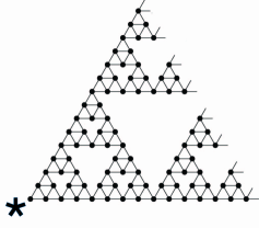
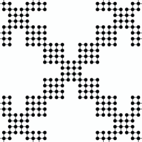
Figure 1. (a) Gasket graph.     (b) Vicsek graph.

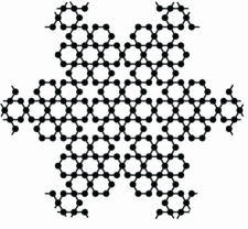
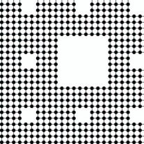
Figure 2. (a) Lindstrom graph.     (b) Carpet graph.

These examples can all be obtained from the following general procedure (for more details, see [6], where the more general case of self-similar CW-complexes has been studied). Assume that we are given a self-similar fractal in ${\mathbb{R}}^{p}$ determined by similarities $w_{1},\ldots,w_{q}$, with the same similarity parameter, and satisfying the Open Set Condition for a bounded open set whose closure is a convex $p$-dimensional polyhedron ${\mathcal{P}}$, and let $K_{1}$ be the graph consisting of the vertices and edges of ${\mathcal{P}}$. If $\sigma=(\sigma_{1},...,\sigma_{n})$ is a multi-index of length $n$, we set $w_{\sigma}:=w_{\sigma_{n}}\circ\cdots\circ w_{\sigma_{1}}$, and assume that $w_{\sigma}{\mathcal{P}}\cap w_{\sigma^{\prime}}{\mathcal{P}}$ is a (facial) subpolyhedron of both $w_{\sigma}{\mathcal{P}}$ and $w_{\sigma^{\prime}}{\mathcal{P}}$, with $|\sigma|=|\sigma^{\prime}|$. Finally, we choose an infinite multi-index $\tau$ and set $K_{n+1}:=\cup_{|\sigma^{\prime}|=n}w_{\tau|_{n}}^{-1}w_{\sigma^{\prime}}K_{1}$, where $\tau|_{n}$ is the multi-index of length $n$ obtained by truncation of $\tau$ to its first $n$ letters. Then $X:=\cup_{n=1}^{\infty}K_{n}$ is a self-similar graph, with amenable exhaustion $\left\{K_{n}\right\}$ and family of local isomorphisms given by ${\mathcal{G}}(n,n+1):=\left\{\gamma_{i}:=w_{\tau|_{n+1}}^{-1}w_{i}w_{\tau|_{n}}:i=1,...,q\right\}$, $n\in{\mathbb{N}}$. Observe that, in the above example 2.4, the generating polyhedron is an equilateral triangle, in the case of the Gasket graph, a square, in the case of the Vicsek or the Carpet graphs, and a regular hexagon, in the case of the Lindstrom graph.

3. A trace on geometric operators

In this section, we construct a trace on the algebra of geometric operators on a self-similar graph. In the following section, this trace will be used to define a determinant on some class of operators on the graph.

Theorem 3.1.

Let $X$ be a self-similar graph, and let ${\mathcal{A}}(X)$ be the C^∗-algebra defined as the norm closure of the ^∗-algebra of geometric operators. Then, on ${\mathcal{A}}(X)$, there is a well-defined trace state $Tr_{{\mathcal{G}}}$ given by

(3.1) $$Tr_{{\mathcal{G}}}(T)=\lim_{n}\frac{Tr\bigl{(}P(K_{n})T\bigr{)}}{Tr\bigl{(}P(K_{n})\bigr{)}},$$

where $P(K_{n})$ is the orthogonal projection of $\ell^{2}(VX)$ onto its closed subspace $\ell^{2}(VK_{n})$.

Proof.

For a finite subset $N\subset VX$, denote by $P(N)$ the orthogonal projection of $\ell^{2}(VX)$ onto $\text{span}(N)$. Let us observe that, since $N$ is an orthonormal basis for $\ell^{2}(N)$, we have $Tr\bigl{(}P(N)\bigr{)}=|N|$. For brevity’s sake, we also use the notation $|K_{n}|:=|VK_{n}|$.

First step: some combinatorial results.

a) Recall that $\displaystyle d=\sup_{v\in VX}|\left\{v^{\prime}\in VX:v^{\prime}\sim v\right\}|$, so that $\displaystyle\sup_{v\in VX}|B_{1}(v)|=d+1$.

Then, since

$$B_{r+1}(v)=\bigcup_{v^{\prime}\in B_{r}(v)}B_{1}(v),$$

we get $|B_{r+1}(v)|\leq(d+1)|B_{r}(v)|$, giving $|B_{r}(v)|\leq(d+1)^{r}$, $\forall v\in VX$, $r\geq 0$. As a consequence, for any finite set $\Omega\subset VX$, we have $B_{r}(\Omega)=\displaystyle\bigcup_{v^{\prime}\in\Omega}B_{r}(v^{\prime})$, giving

(3.2) $$|B_{r}(\Omega)|\leq|\Omega|(d+1)^{r},\quad\forall r\geq 0.$$

b) Let us set $\Omega_{n,r}=VK_{n}\setminus B_{r}({\mathcal{F}}_{{\mathcal{G}}}(K_{n}))$. Then, for any $\gamma\in{\mathcal{G}}(n)$, we have

(3.3) $$\gamma\Omega_{n,r}\subset\gamma VK_{n}=V(\gamma K_{n})\subset\gamma\Omega_{n,r}\cup B_{r}({\mathcal{F}}_{{\mathcal{G}}}(\gamma K_{n})).$$

Now assume $r\geq 1$. Then the $\gamma\Omega_{n,r}$’s are disjoint for different $\gamma$’s in ${\mathcal{G}}(n,m)$. Therefore

(3.4) $$|K_{n}| \leq|\Omega_{n,r}|+|{\mathcal{F}}_{{\mathcal{G}}}(K_{n})|(d+1)^{r},$$

(3.5) $$\left|VK_{m}\setminus\bigcup_{\gamma\in{\mathcal{G}}(n,m)}\gamma\Omega_{n,r}\right| \leq|{\mathcal{G}}(n,m)|\,|{\mathcal{F}}_{{\mathcal{G}}}(K_{n})|(d+1)^{r},$$

(3.6) $$|{\mathcal{G}}(n,m)|\,|\Omega_{n,r}| \leq|K_{m}|\leq|{\mathcal{G}}(n,m)|\,|K_{n}|.$$

Indeed, (3.4) and (3.6) are easily verified, while

$$\left|VK_{m}\setminus\bigcup_{\gamma\in{\mathcal{G}}(n,m)}\gamma\Omega_{n,r}\right| =\left|\bigcup_{\gamma\in{\mathcal{G}}(n,m)}\gamma VK_{n}\setminus\bigcup_{\gamma\in{\mathcal{G}}(n,m)}\gamma\Omega_{n,r}\right|$$

$$\leq\sum_{\gamma\in{\mathcal{G}}(n,m)}\left|\gamma[VK_{n}\setminus\Omega_{n,r}]\right|$$

$$\leq|{\mathcal{G}}(n,m)|\left|B_{r}({\mathcal{F}}_{{\mathcal{G}}}(K_{n}))\right|$$

$$\leq|{\mathcal{G}}(n,m)|\left|{\mathcal{F}}_{{\mathcal{G}}}(K_{n})\right|(d+1)^{r}.$$

c) Set $\varepsilon_{n}=\displaystyle{\frac{|{\mathcal{F}}_{{\mathcal{G}}}(K_{n})|}{|K_{n}|}}$ and recall that, by assumption, $\varepsilon_{n}\to 0$. Putting together (3.4) and (3.6), we get

$$|{\mathcal{G}}(n,m)|\,|K_{n}|-|{\mathcal{G}}(n,m)|\,|{\mathcal{F}}_{{\mathcal{G}}}(K_{n})|(d+1)^{r}\leq|K_{m}|\leq|{\mathcal{G}}(n,m)|\,|K_{n}|,$$

which implies

(3.7) $$1-\varepsilon_{n}(d+1)^{r}\leq\frac{|K_{m}|}{|{\mathcal{G}}(n,m)|\,|K_{n}|}\leq 1.$$

Choosing $n_{0}$ such that for all $n>n_{0}$, $\varepsilon_{n}(d+1)^{r}\leq 1/2$, we obtain

(3.8) $$0\leq\frac{|{\mathcal{G}}(n,m)|\,|K_{n}|}{|K_{m}|}-1\leq 2\varepsilon_{n}(d+1)^{r}\leq 1.$$

Therefore, we deduce from (3.5) that

(3.9) $$\left|VK_{m}\setminus\bigcup_{\gamma\in{\mathcal{G}}(n,m)}\gamma\Omega_{n,r}\right| \leq|{\mathcal{G}}(n,m)|\left|{\mathcal{F}}_{{\mathcal{G}}}(K_{n})\right|(d+1)^{r}$$

$$=|{\mathcal{G}}(n,m)|\left|K_{n}\right|\varepsilon_{n}(d+1)^{r}\leq 2\left|K_{m}\right|\varepsilon_{n}(d+1)^{r}.$$

Second step: the existence of the limit for geometric operators.

a) By definition of $U(\gamma)$, we have, for $\gamma\in{\mathcal{G}}(n,m)$, with $n<m$,

(3.10) $$U^{*}(\gamma)U(\gamma)=P(VK_{n}),\qquad U(\gamma)U^{*}(\gamma)=P(\gamma VK_{n}).$$

Assume now that $T$ is a geometric operator on $\ell^{2}(VX)$with finite propagation $r$. Then $TU(\gamma)P(\Omega_{n,r})=U(\gamma)TP(\Omega_{n,r})$ and $P(\gamma\Omega_{n,r})=U(\gamma)P(\Omega_{n,r})U(\gamma)^{*}$. Hence,

(3.11) $$Tr\bigl{(}TP(\gamma\Omega_{n,r})\bigr{)} =Tr\bigl{(}TU(\gamma)P(\Omega_{n,r})U(\gamma)^{*}\bigr{)}$$

$$=Tr\bigl{(}U(\gamma)TP(\Omega_{n,r})U(\gamma)^{*}\bigr{)}$$

$$=Tr\bigl{(}TP(\Omega_{n,r})U(\gamma)^{*}U(\gamma)\bigr{)}$$

$$=Tr\bigl{(}TP(\Omega_{n,r})P(VK_{n})\bigr{)}=Tr\bigl{(}TP(\Omega_{n,r})\bigr{)}.$$

b) Let us show that the sequence is Cauchy:

$$\left|\frac{TrTP(VK_{n})}{TrP(VK_{n})}-\frac{TrTP(VK_{m})}{TrP(VK_{m})}\right|\leq$$

$$\leq\frac{|TrT(P(VK_{n})-P(\Omega_{n,r}))|}{|K_{n}|}+\frac{|TrT(P(VK_{m})-P(\cup_{\gamma\in{\mathcal{G}}(n,m)}\gamma\Omega_{n,r}))|}{|K_{m}|}$$

$$\qquad+\left|\frac{TrTP(\Omega_{n,r})}{|K_{n}|}-\frac{|{\mathcal{G}}(n,m)|\,|K_{n}|}{|K_{m}|}\frac{TrTP(\Omega_{n,r})}{|K_{n}|}\right|$$

$$\leq\|T\|\left(\frac{|VK_{n}\setminus\Omega_{n,r}|}{|K_{n}|}+\frac{|VK_{m}\setminus\cup_{\gamma\in{\mathcal{G}}(n,m)}\gamma\Omega_{n,r}|}{|K_{m}|}+\left|1-\frac{|{\mathcal{G}}(n,m)|\,|K_{n}|}{|K_{m}|}\right|\right)$$

$$\leq 5\|T\|\varepsilon_{n}(d+1)^{r},$$

where we used (3.11), in the first inequality, and (3.2), (3.9), (3.8), in the third inequality.

Third step: $Tr_{{\mathcal{G}}}$ is a state on ${\mathcal{A}}(X)$.

a) Let $T\in{\mathcal{A}}(X)$, $\varepsilon>0$. Since ${\mathcal{A}}(X)$ is the norm closure of the ^∗-algebra of geometric operators, we can find a geometric operator $T^{\prime}\in{\mathcal{A}}_{g}(X)$ such that $\|T-T^{\prime}\|\leq\varepsilon/3$. Further, set $\phi_{n}(A):=\frac{TrAP(VK_{n})}{TrP(VK_{n})}$. Then choose $n$ such that, for every $m>n$, $|\phi_{m}(T^{\prime})-\phi_{n}(T^{\prime})|\leq\varepsilon/3$. We get

$$|\phi_{m}(T)-\phi_{n}(T)|\leq|\phi_{m}(T-T^{\prime})|+|\phi_{m}(T^{\prime})-\phi_{n}(T^{\prime})|+|\phi_{n}(T-T^{\prime})|\leq\varepsilon.$$

Hence, we have proved that $\lim\phi_{n}(T)$ exists.

b) The functional $Tr_{{\mathcal{G}}}$ is clearly linear, positive and takes value $1$ on the identity, hence it is a state on ${\mathcal{A}}(X)$.

Fourth step: $Tr_{{\mathcal{G}}}$ is a trace on ${\mathcal{A}}(X)$.

Let $A$ be a geometric operator with propagation $r$. Then

$$AP(VK_{n}) =P(B_{r}(VK_{n}))AP(VK_{n}),$$

$$P(\Omega_{n,r})A =P(\Omega_{n,r})AP(VK_{n}).$$

Indeed, the first equality is easily verified. As for the second, we have

$$\Omega_{n,r}\subset VK_{n}\setminus B_{r}({\mathcal{F}}(K_{n}))=\left\{v\in VK_{n}:\rho(v,VX\setminus VK_{n})\geq r+2\right\},$$

so that

$$B_{r}(\Omega_{n,r})\subset\left\{v\in VK_{n}:\rho(v,VX\setminus VK_{n})\geq 2\right\}\subset VK_{n}.$$

Since $A^{*}$ has propagation $r$, we get

$$A^{*}P(\Omega_{n,r})=P(B_{r}(\Omega_{n,r}))A^{*}P(\Omega_{n,r})=P(VK_{n})A^{*}P(\Omega_{n,r}),$$

which proves the claim. Hence,

$$AP(VK_{n})=P(B_{r}(VK_{n})\setminus\Omega_{n,r})AP(VK_{n})+P(\Omega_{n,r})A$$

$$=P(B_{r}(VK_{n})\setminus\Omega_{n,r})AP(VK_{n})-P(VK_{n}\setminus\Omega_{n,r})A+P(VK_{n})A.$$

Therefore, if $B\in{\mathcal{A}}(X)$,

$$\phi_{n}([B,A]) \leq\|A\|\,\|B\|\frac{|B_{r}(VK_{n})\setminus\Omega_{n,r}|+|VK_{n}\setminus\Omega_{n,r}|}{|K_{n}|}$$

$$\leq 2\|A\|\,\|B\|\varepsilon_{n}(d+1)^{r},$$

since $B_{r}(VK_{n})\setminus\Omega_{n,r}\subset B_{r}({\mathcal{F}}_{{\mathcal{G}}}(K_{n}))$. Taking the limit as $n\to\infty$, we deduce that $Tr_{{\mathcal{G}}}([B,A])=0$. By continuity, it follows that the result holds for any $A,B\in{\mathcal{A}}(X)$. ∎

Remark 3.2.

Let us note that the trace described in the previous theorem is not faithful in general. For example, for the Gasket graph in figure 1a the trace of $4I-D$ vanishes.

4. An analytic determinant for C^∗-algebras with a trace state

In this section, we define a determinant for a suitable class of not necessarily normal operators in a C^∗-algebra with a trace state, cf. [43] for related results. The results obtained are used in Section 7 to prove a determinant formula for the zeta function.

In a celebrated paper [12], Fuglede and Kadison defined a positive-valued determinant for finite factors ($i.e.$ von Neumann algebras with trivial center and finite trace). Such a determinant is defined on all invertible elements and enjoys the main properties of a determinant function, but it is positive-valued. Indeed, for an invertible operator $A$ with polar decomposition $A=UH$, where $U$ is a unitary operator and $H:=\sqrt{A^{*}A}$ is a positive self-adjoint operator, the Fuglede–Kadison determinant is defined by

$$Det(A)=\exp\,\circ\ \tau\circ\log H,$$

where $\log H$ may be defined via the functional calculus.

For the purposes of the present paper, we need a determinant which is an analytic function. As we shall see, this can be achieved but corresponds to a restriction of the domain of the determinant function and implies the loss of some important properties. Let $({\mathcal{A}},\tau)$ be a C^∗-algebra endowed with a trace state. Then, a natural way to obtain an analytic function is to define, for $A\in{\mathcal{A}}$, $\text{det}_{\tau}(A)=\exp\,\circ\ \tau\circ\log A$, where

$$\log(A):=\frac{1}{2\pi i}\int_{\Gamma}\log\lambda(\lambda-A)^{-1}d\lambda$$

and $\Gamma$ is the boundary of a connected, simply connected region $\Omega$ containing the spectrum of $A$. Clearly, once the branch of the logarithm is chosen, the integral above does not depend on $\Gamma$, provided $\Gamma$ is given as above.

Then a naïve way of defining $det$ is to allow all elements $A$ for which there exists an $\Omega$ as above and a branch of the logarithm whose domain contains $\Omega$. Indeed, the following holds.

Lemma 4.1.

Let $A$, $\Omega$, $\Gamma$ be as above, and $\varphi$, $\psi$ two branches of the logarithm such that both associated domains contain $\Omega$. Then

$$\exp\,\circ\ \tau\circ\varphi(A)=\exp\,\circ\ \tau\circ\psi(A).$$

Proof.

The function $\varphi(\lambda)-\psi(\lambda)$ is continuous and everywhere defined on $\Gamma$. Since it takes its values in $2\pi i\mathbb{Z}$, it should be constant on $\Gamma$. Therefore,

$$\exp\,\circ\ \tau\circ\varphi(A) =\exp\,\circ\ \tau\left(\frac{1}{2\pi i}\int_{\Gamma}2\pi in_{0}(\lambda-A)^{-1}d\lambda\right)\exp\,\circ\ \tau\circ\psi(A)$$

$$=\exp\,\circ\ \tau\circ\psi(A).$$

∎

The problem with the previous definition is its dependence on the choice of $\Omega$. Indeed, it is easy to see that when $A=\begin{pmatrix}1&0\\ 0&i\end{pmatrix}$, and if we choose $\Omega$ containing $\{e^{i\vartheta},\vartheta\in[0,\pi/2]\}$ and any suitable branch of the logarithm, the determinant defined in terms of the normalized trace gives $det(A)=e^{i\pi/4}$. On the other hand, if we choose $\Omega$ containing $\{e^{i\vartheta},\vartheta\in[\pi/2,2\pi]\}$ and a corresponding branch of the logarithm, we have $det(A)=e^{5i\pi/4}$. Hence, we make the following choice.

Definition 4.2.

Let $({\mathcal{A}},\tau)$ be a C^∗-algebra endowed with a trace state, and consider the subset ${\mathcal{A}}_{0}:=\{A\in{\mathcal{A}}:0\not\in\text{conv}\,\sigma(A)\}$, where $\sigma(A)$ denotes the spectrum of $A$ and $\text{conv}\,\sigma(A)$ its convex hull. For any $A\in{\mathcal{A}}_{0}$ we set

$$\text{det}_{\tau}(A)=\exp\,\circ\ \tau\circ\left(\frac{1}{2\pi i}\int_{\Gamma}\log\lambda(\lambda-A)^{-1}d\lambda\right),$$

where $\Gamma$ is the boundary of a connected, simply connected region $\Omega$ containing $\text{conv}\,\sigma(A)$, and $\log$ is a branch of the logarithm whose domain contains $\Omega$.

Since two $\Gamma$’s as above are homotopic in ${\mathbb{C}}\setminus\text{conv}\,\sigma(A)$, we have

Corollary 4.3.

The determinant function defined above is well-defined and analytic on ${\mathcal{A}}_{0}$.

We collect several properties of our determinant in the following result.

Proposition 4.4.

Let $({\mathcal{A}},\tau)$ be a C^∗-algebra endowed with a trace state, and let $A\in{\mathcal{A}}_{0}$. Then

$\text{det}_{\tau}(zA)=z\text{det}_{\tau}(A)$, for any $z\in\mathbb{C}\setminus\{0\}$,

if $A$ is normal, and $A=UH$ is its polar decomposition,

$$\text{det}_{\tau}(A)=\text{det}_{\tau}(U)\text{det}_{\tau}(H),$$

if $A$ is positive, then we have $\text{det}_{\tau}(A)=Det(A)$, where the latter is the Fuglede–Kadison determinant.

Proof.

$(i)$ If, for a given $\vartheta_{0}\in[0,2\pi)$, the half-line $\{\rho e^{i\vartheta_{0}}\in\mathbb{C}:\rho>0\}$ does not intersect $\text{conv}\,\sigma(A)$, then the half-line $\{\rho e^{i(\vartheta_{0}+t)}\in\mathbb{C}:\rho>0\}$ does not intersect $\text{conv}\,\sigma(zA)$, where $z=re^{it}$. If $\log$ is the branch of the logarithm defined on the complement of the real negative half-line, then $\varphi(x)=i(\vartheta_{0}-\pi)+\log(e^{-i(\vartheta_{0}-\pi)}x)$ is suitable for defining $\text{det}_{\tau}(A)$, while $\psi(x)=i(\vartheta_{0}+t-\pi)+\log(e^{-i(\vartheta_{0}+t-\pi)}x)$ is suitable for defining $\text{det}_{\tau}(zA)$. Moreover, if $\Gamma$ is the boundary of a connected, simply connected region $\Omega$ containing $\text{conv}\,\sigma(A)$, then $z\Gamma$ is the boundary of a connected, simply connected region $z\Omega$ containing $\text{conv}\,\sigma(zA)$. Therefore,

$$\text{det}_{\tau}(zA) =\exp\,\circ\ \tau\left(\frac{1}{2\pi i}\int_{z\Gamma}\psi(\lambda)(\lambda-zA)^{-1}d\lambda\right)$$

$$=\exp\,\circ\ \tau\left(\frac{1}{2\pi i}\int_{\Gamma}(i(\vartheta_{0}+t-\pi)+\log(e^{-i(\vartheta_{0}+t-\pi)}re^{it}\mu))(\mu-A)^{-1}d\mu\right)$$

$$=\exp\,\circ\ \tau\left((\log r+it)I+\frac{1}{2\pi i}\int_{\Gamma}\varphi(\mu)(\mu-A)^{-1}d\mu\right)$$

$$=z\text{det}_{\tau}(A).$$

$(ii)$ When $A=UH$ is normal, $U=\int_{[0,2\pi]}e^{i\vartheta}\ du(\vartheta)$, $H=\int_{[0,\infty)}r\ dh(r)$, then $A=\int_{[0,\infty)\times[0,2\pi]}re^{i\vartheta}\ d(h(r)\otimes u(\vartheta))$. The property $0\not\in\text{conv}\,\sigma(A)$ is equivalent to the fact that the support of the measure $d(h(r)\otimes u(\vartheta))$ is compactly contained in some open half-plane

$$\{\rho e^{i\vartheta}:\rho>0,\vartheta\in(\vartheta_{0}-\pi/2,\vartheta_{0}+\pi/2)\},$$

or, equivalently, that the support of the measure $dh(r)$ is compactly contained in $(0,\infty)$ and the support of the measure $du(\vartheta)$ is compactly contained in $(\vartheta_{0}-\pi/2,\vartheta_{0}+\pi/2)$. Thus, $A\in{\mathcal{A}}_{0}$ is equivalent to $U,H\in{\mathcal{A}}_{0}$. Then

$$\log A=\int_{[0,\infty)\times(\vartheta_{0}-\pi/2,\vartheta_{0}+\pi/2)}(\log r+i\vartheta)\ d(h(r)\otimes u(\vartheta)),$$

which implies that

$$\text{det}_{\tau}(A) =\exp\,\circ\ \tau\left(\int_{0}^{\infty}\log r\ dh(r)+\int_{\vartheta_{0}-\pi/2}^{\vartheta_{0}+\pi/2}i\vartheta\ du(\vartheta)\right)$$

$$=\text{det}_{\tau}(U)\cdot\text{det}_{\tau}(H).$$

$(iii)$ This follows by the argument given in $(ii)$. ∎

Remark 4.5.

We note that the above defined determinant function strongly violates the product property $\text{det}_{\tau}(AB)=\text{det}_{\tau}(A)\text{det}_{\tau}(B)$. Firstly, $A,B\in{\mathcal{A}}_{0}$ does not imply $AB\in{\mathcal{A}}_{0}$, as is seen e.g. by taking $A=B=\begin{pmatrix}1&0\\ 0&i\end{pmatrix}$. Moreover, even if $A,B,AB\in{\mathcal{A}}_{0}$ and $A$ and $B$ commute, the product property may be violated, as is shown by choosing $A=B=\begin{pmatrix}1&0\\ 0&e^{3i\pi/4}\end{pmatrix}$ and using the normalized trace on $2\times 2$ matrices.

5. Reduced closed paths

The Ihara zeta function is defined by means of equivalence classes of prime cycles. Therefore, we need to introduce some terminology from graph theory, following [39], with some suitable modifications. Moreover, we provide several technical results that will be used in the following sections. We note that our approach to the determinant formula, here and in the following two sections, is inspired by the simplification brought to the subject by Stark and Terras in [39].

Recall that a path (of length $m$) in $X$ from $v_{0}\in VX$ to $v_{m}\in VX$ is given by $(v_{0},\ldots,v_{m})$, where $v_{i}\in VX$, $v_{i+1}\sim v_{i}$, for $i=0,...,m-1$. A path is closed if $v_{m}=v_{0}$. Let us notice that an initial point $v_{0}$ is assigned also if the path is closed.

Definition 5.1 (Proper closed Paths).

$(i)$ A path in $X$ has backtracking if $v_{i-1}=v_{i+1}$, for some $i\in\{1,\ldots,m-1\}$. A path with no backtracking is also called proper. Denote by ${\mathcal{C}}$ the set of proper closed paths, and by ${\mathcal{C}}_{m}$ the subset given by paths of length $m$.

$(ii)$ A proper closed path $C=(v_{0},\ldots,v_{m}=v_{0})$ has a tail if there is $k\in\{1,\ldots,[\frac{m}{2}]-1\}$ such that $v_{j}=v_{m-j}$, for $j=1,\ldots,k$. Denote by ${\mathcal{C}}^{\mathrm{tail}}$ the set of proper closed paths with tail, and by ${\mathcal{C}}^{\mathrm{notail}}$ the set of proper tail-less closed paths, also called reduced closed paths. The symbols ${\mathcal{C}}^{\mathrm{tail}}_{m}$ and ${\mathcal{C}}^{\mathrm{notail}}_{m}$ will denote the corresponding subsets of paths of length $m$. Observe that ${\mathcal{C}}={\mathcal{C}}^{\mathrm{tail}}\cup{\mathcal{C}}^{\mathrm{notail}}$, ${\mathcal{C}}^{\mathrm{tail}}\cap{\mathcal{C}}^{\mathrm{notail}}=\emptyset$.

$(iii)$ A reduced closed path is primitive if it is not obtained by going $n\geq 2$ times around some other closed path.

Let us denote by $A$ the adjacency matrix of $X$, as defined in (1.3). For any $m\in{\mathbb{N}}$, let us denote by $A_{m}(x,y)$ the number of proper paths in $X$, of length $m$, with initial vertex $x$ and terminal vertex $y$, for $x,y\in VX$. Then $A_{1}=A$. Let $A_{0}:=I$, and set $Q=D-I$, where $D$ is given by (1.4). Then, we obtain

Lemma 5.2.

$(i)$ $A_{2}=A^{2}-Q-I\in{\mathcal{A}}(X)$,

$(ii)$ for $m\geq 3$, $A_{m}=A_{m-1}A-A_{m-2}Q\in{\mathcal{A}}(X)$,

$(iii)$ if we let $d:=\sup_{v\in VX}\deg(v)$ and $\alpha:=\frac{d+\sqrt{d^{2}+4d}}{2}$, we have $\|A_{m}\|\leq\alpha^{m}$, for $m\geq 0$.

Proof.

$(i)$ If $x=y$ then $A_{2}(x,y)=0$ and $A^{2}(x,x)=deg(x)=(Q+I)(x,x)$. If $x\neq y$, $A_{2}(x,y)=A(x,y)$ and $(Q+I)(x,y)=0$.

$(ii)$ For $x,y\in VX$, the sum $\sum_{z\in VX}A_{m-1}(x,z)A(z,y)$ counts the proper paths of length $m$ from $x$ to $y$, which are $A_{m}(x,y)$, plus the paths of length $m$ from $x$ to $y$ with backtracking at the end. The paths in the latter family consist of a proper path of length $m-2$ from $x$ to $y$ followed by a path of length $2$ from $y$ to $z$ and back; to avoid further backtracking, there are only $Q(y,y)$ choices for $z$, namely there are $A_{m-2}(x,y)Q(y,y)$ such paths.

$(iii)$ We have $\|A_{1}\|=\|A\|\leq d$, $\|A_{2}\|\leq d^{2}+d$, and $\|A_{m}\|\leq d(\|A_{m-1}\|+\|A_{m-2}\|)$, from which the claim follows by induction. ∎

Lemma 5.3.

For $m\in{\mathbb{N}}$, let

$$t_{m}:=\lim_{n\to\infty}\frac{1}{|K_{n}|}\sum_{x\in K_{n}}\left|\left\{C\in{\mathcal{C}}^{\mathrm{tail}}_{m}:C\text{ starts at }x\right\}\right|.$$

Then

$(i)$ the above limit exists and is finite,

$(ii)$ $t_{1}=t_{2}=0$, and, for $m\geq 3$, $t_{m}=t_{m-2}+Tr_{{\mathcal{G}}}((Q-I)A_{m-2})$,

$(iii)$ $t_{m}=Tr_{{\mathcal{G}}}\left((Q-I)\sum_{j=1}^{[\frac{m-1}{2}]}A_{m-2j}\right)$, where $Tr_{{\mathcal{G}}}$ is defined in Theorem 3.1.

Proof.

Denote by $(C,v)$ the proper closed path $C$ with the origin in $v\in VX$.

$(i)$ For $n\in{\mathbb{N}}$, let

$$\Omega_{n}:=V(K_{n})\setminus B_{1}({\mathcal{F}}_{\mathcal{G}}(K_{n})),\qquad\Omega_{n}^{\prime}:=B_{1}({\mathcal{F}}_{{\mathcal{G}}}(K_{n}))\cap V(K_{n}).$$

Then, for all $p\in{\mathbb{N}}$,

$$V(K_{n+p})=\left(\bigcup_{\gamma\in{\mathcal{G}}(n,n+p)}\gamma\Omega_{n}\right)\cup\left(\bigcup_{\gamma\in{\mathcal{G}}(n,n+p)}\gamma\Omega_{n}^{\prime}\right).$$

Let $t_{m}(x):=|\left\{(C,x)\in{\mathcal{C}}^{\mathrm{tail}}_{m}\right\}|\leq d(d-1)^{m-2}$. Then

$$\left|\frac{1}{|K_{n+p}|}\sum_{x\in K_{n+p}}t_{m}(x)-\frac{1}{|K_{n}|}\sum_{x\in K_{n}}t_{m}(x)\right|$$

$$\leq\left|\frac{|{\mathcal{G}}(n,n+p)|}{|K_{n+p}|}\sum_{x\in\Omega_{n}}t_{m}(x)-\frac{1}{|K_{n}|}\sum_{x\in K_{n}}t_{m}(x)\right|+\frac{|{\mathcal{G}}(n,n+p)|}{|K_{n+p}|}\sum_{x\in\Omega_{n}^{\prime}}t_{m}(x)$$

$$\leq\left|\frac{|{\mathcal{G}}(n,n+p)|}{|K_{n+p}|}-\frac{1}{|K_{n}|}\right|\sum_{x\in K_{n}}t_{m}(x)+2\frac{|{\mathcal{G}}(n,n+p)|}{|K_{n+p}|}\sum_{x\in B_{1}({\mathcal{F}}_{\mathcal{G}}(K_{n}))}t_{m}(x)$$

$$\leq\left|1-\frac{|K_{n}||{\mathcal{G}}(n,n+p)|}{|K_{n+p}|}\right|d(d-1)^{m-2}+2\frac{|K_{n}||{\mathcal{G}}(n,n+p)|}{|K_{n+p}|}\frac{|B_{1}({\mathcal{F}}_{\mathcal{G}}(K_{n}))|}{|K_{n}|}d(d-1)^{m-2}$$

$$\leq 6(d-1)^{m-2}d(d+1)\varepsilon_{n}\to 0,\quad\text{ as }n\to\infty,$$

where, in the last inequality, we used equations (3.2), (3.8) [with $r=1$], and the fact that $\varepsilon_{n}=\displaystyle\frac{|{\mathcal{F}}_{\mathcal{G}}(K_{n})|}{|K_{n}|}\to 0$.

$(ii)$ Let us define $\Omega:=\left\{v\in VX:v\not\in K_{n},\rho(v,K_{n})=1\right\}\subset B_{1}({\mathcal{F}}_{\mathcal{G}}(K_{n}))$. We have

$$\frac{1}{|K_{n}|}\sum_{x\in K_{n}}\sum_{y\sim x} |\left\{C=(x,y,...)\in{\mathcal{C}}^{\mathrm{tail}}_{m}\right\}|=$$

$$=\frac{1}{|K_{n}|}\sum_{y\in K_{n}}\sum_{x\sim y}|\left\{C=(x,y,...)\in{\mathcal{C}}^{\mathrm{tail}}_{m}\right\}|$$

$$\quad+\frac{1}{|K_{n}|}\sum_{y\in\Omega}\sum_{x\in K_{n},x\sim y}|\left\{C=(x,y,...)\in{\mathcal{C}}^{\mathrm{tail}}_{m}\right\}|$$

$$\quad-\frac{1}{|K_{n}|}\sum_{y\in K_{n}}\sum_{x\in\Omega,x\sim y}|\left\{C=(x,y,...)\in{\mathcal{C}}^{\mathrm{tail}}_{m}\right\}|.$$

Since

$$\frac{1}{|K_{n}|}\sum_{y\in\Omega}\sum_{x\in K_{n},x\sim y}|\left\{C=(x,y,...)\in{\mathcal{C}}^{\mathrm{tail}}_{m}\right\}|\leq\frac{1}{|K_{n}|}|{\mathcal{F}}_{\mathcal{G}}(K_{n})|d(d+1)(d-1)^{m-2}\to 0$$

and

$$\frac{1}{|K_{n}|}\sum_{y\in K_{n}}\sum_{x\in\Omega,x\sim y} |\left\{C=(x,y,...)\in{\mathcal{C}}^{\mathrm{tail}}_{m}\right\}|=$$

$$=\frac{1}{|K_{n}|}\sum_{y\in{\mathcal{F}}_{\mathcal{G}}(K_{n})}\sum_{x\in\Omega,x\sim y}|\left\{C=(x,y,...)\in{\mathcal{C}}^{\mathrm{tail}}_{m}\right\}|$$

$$\leq\frac{1}{|K_{n}|}|{\mathcal{F}}_{\mathcal{G}}(K_{n})|d(d-1)^{m-2}\to 0,$$

we obtain

$$t_{m} =\lim_{n\to\infty}\frac{1}{|K_{n}|}\sum_{x\in K_{n}}|\left\{(C,x)\in{\mathcal{C}}^{\mathrm{tail}}_{m}\right\}|$$

$$=\lim_{n\to\infty}\frac{1}{|K_{n}|}\sum_{x\in K_{n}}\sum_{y\sim x}|\left\{C=(x,y,...)\in{\mathcal{C}}^{\mathrm{tail}}_{m}\right\}|$$

$$=\lim_{n\to\infty}\frac{1}{|K_{n}|}\sum_{y\in K_{n}}\sum_{x\sim y}|\left\{C=(x,y,...)\in{\mathcal{C}}^{\mathrm{tail}}_{m}\right\}|.$$

For a given $y$, we now want to count the paths in ${\mathcal{C}}^{\mathrm{tail}}_{m}$ whose second vertex is $y$. Any such path can be identified by the choice of a first vertex $x\sim y$ and a proper closed path $D$ of length $(m-2)$. Of course we may first choose the closed path $D$ and then the first vertex $x$. There are two kinds of proper closed paths $D$ starting at $y$, namely, those with tails and those without. If $D$ has no tail, then there are $Q(y,y)-1$ possibilities for $x$ to be adjacent to $y$ in such a way that the resulting path $C$ has no backtracking. If $D$ has a tail, then there are $Q(y,y)$ possibilities for $x$ to be adjacent to $y$ in such a way that the resulting path $C$ has no backtracking. Therefore, we have

$$\sum_{x\sim y} |\left\{C=(x,y,...)\in{\mathcal{C}}^{\mathrm{tail}}_{m}\right\}|=$$

$$=(Q(y,y)-1)\cdot|\left\{(D,y)\in{\mathcal{C}}^{\mathrm{notail}}_{m-2}\right\}|+Q(y,y)\cdot|\left\{(D,y)\in{\mathcal{C}}^{\mathrm{tail}}_{m-2}\right\}|$$

$$=(Q(y,y)-1)\cdot|\left\{(D,y)\in{\mathcal{C}}_{m-2}\right\}|+|\left\{(D,y)\in{\mathcal{C}}^{\mathrm{tail}}_{m-2}\right\}|\,,$$

so that

$$t_{m} =\lim_{n\to\infty}\frac{1}{|K_{n}|}\sum_{y\in K_{n}}(Q(y,y)-1)\cdot|\left\{(D,y)\in{\mathcal{C}}_{m-2}\right\}|$$

$$\qquad+\lim_{n\to\infty}\frac{1}{|K_{n}|}\sum_{y\in K_{n}}|\left\{(D,y)\in{\mathcal{C}}^{\mathrm{tail}}_{m-2}\right\}|$$

$$=\lim_{n\to\infty}\frac{1}{|K_{n}|}\sum_{y\in K_{n}}(Q(y,y)-1)A_{m-2}(y,y)+t_{m-2}$$

$$=Tr_{{\mathcal{G}}}((Q-I)A_{m-2})+t_{m-2}.$$

$(iii)$ This follows from $(ii)$. ∎

Lemma 5.4.

Let

$$N_{m}:=\lim_{n\to\infty}\frac{1}{|K_{n}|}|\left\{C\in{\mathcal{C}}^{\mathrm{notail}}_{m}:C\subset K_{n}\right\}|,$$

which exists and is finite. Then, for all $m\in{\mathbb{N}}$,

$(i)$ $N_{m}=Tr_{{\mathcal{G}}}(A_{m})-t_{m}$,

$(ii)$ $N_{m}\leq d(d-1)^{m-1}$.

Proof.

$(i)$ Observe that

(5.1) $$N_{m}=\lim_{n\to\infty}\frac{1}{|K_{n}|}|\left\{(C,v)\in{\mathcal{C}}^{\mathrm{notail}}_{m}:v\in K_{n}\right\}|.$$

Indeed,

$$0 \leq\frac{1}{|K_{n}|}\Big{|}|\left\{(C,v)\in{\mathcal{C}}^{\mathrm{notail}}_{m}:v\in K_{n}\right\}|-|\left\{C\in{\mathcal{C}}^{\mathrm{notail}}_{m}:C\subset K_{n}\right\}|\Big{|}$$

$$=\frac{1}{|K_{n}|}\,\left|\left\{(C,v)\in{\mathcal{C}}^{\mathrm{notail}}_{m}:v\in K_{n},C\not\subset K_{n}\right\}\right|$$

$$\leq\frac{1}{|K_{n}|}\,\left|\left\{(C,v)\in{\mathcal{C}}_{m}:v\in B_{m}({\mathcal{F}}_{\mathcal{G}}(K_{n}))\right\}\right|$$

$$=\frac{1}{|K_{n}|}\,\sum_{v\in B_{m}({\mathcal{F}}_{\mathcal{G}}(K_{n}))}A_{m}(v,v)=\frac{1}{|K_{n}|}\,Tr(P(B_{m}({\mathcal{F}}_{\mathcal{G}}(K_{n})))A_{m})$$

$$\leq\|A_{m}\|\,\frac{|B_{m}({\mathcal{F}}_{\mathcal{G}}(K_{n}))|}{|K_{n}|}\leq\|A_{m}\|\,(d+1)^{m}\frac{|{\mathcal{F}}_{\mathcal{G}}(K_{n})|}{|K_{n}|}\to 0,\,\text{as }n\to\infty.$$

Moreover, the existence of $\lim_{n\to\infty}\frac{1}{|K_{n}|}|\left\{(C,v)\in{\mathcal{C}}^{\mathrm{notail}}_{m}:v\in K_{n}\right\}|$ can be proved as in Lemma 5.3 $(i)$. Therefore,

$$N_{m} =\lim_{n\to\infty}\frac{1}{|K_{n}|}\left|\left\{(C,v)\in{\mathcal{C}}^{\mathrm{notail}}_{m}:v\in K_{n}\right\}\right|$$

$$=\lim_{n\to\infty}\frac{1}{|K_{n}|}\,\biggl{(}\sum_{v\in K_{n}}A_{m}(v,v)-\sum_{v\in K_{n}}\left|\left\{(C,v)\in{\mathcal{C}}^{\mathrm{tail}}_{m}:v\in K_{n}\right\}\right|\biggr{)}$$

$$=Tr_{{\mathcal{G}}}(A_{m})-t_{m}.$$

$(ii)$ This follows from (5.1). ∎

6. The Zeta function

In this section, we define the Ihara zeta function for a self-similar graph and prove that it is a holomorphic function in a suitable disc. We first need to introduce some equivalence relations between closed paths.

Definition 6.1 (Cycles).

We say that two closed paths $C=(v_{0},\ldots,v_{m}=v_{0})$ and $D=(w_{0},\ldots,w_{m}=w_{0})$ are equivalent, and write $C\sim_{o}D$, if there is an integer $k$ such that $w_{j}=v_{j+k}$, for all $j$, where the addition is taken modulo $m$, that is, the origin of $D$ is shifted $k$ steps with respect to the origin of $C$. The equivalence class of $C$ is denoted $[C]_{o}$. An equivalence class is also called a cycle. Therefore, a closed path is just a cycle with a specified origin.

Denote by ${\mathcal{R}}$ the set of reduced cycles, and by ${\mathcal{P}}\subset{\mathcal{R}}$ the subset of primitive reduced cycles, also called prime cycles.

Definition 6.2 (Equivalence relation between reduced cycles).

Given $C$, $D\in{\mathcal{R}}$, we say that $C$ and $D$ are ${\mathcal{G}}$-equivalent, and write $C\sim_{{\mathcal{G}}}D$, if there is a local isomorphism $\gamma\in{\mathcal{G}}$ such that $D=\gamma(C)$. We denote by $[{\mathcal{R}}]_{{\mathcal{G}}}$ the set of ${\mathcal{G}}$-equivalence classes of reduced cycles, and analogously for the subset ${\mathcal{P}}$.

We need to introduce several quantities associated to a reduced cycle.

Definition 6.3 (Average multiplicity of a reduced cycle).

Let $C\in{\mathcal{R}}$, and call

$(i)$ size of $C$, denoted $s(C)\in{\mathbb{N}}$, the least $m\in{\mathbb{N}}$ such that $C\subset\gamma(K_{m})$, for some local isomorphism $\gamma\in{\mathcal{G}}(m)$,

$(ii)$ effective length of $C$, denoted $\ell(C)\in{\mathbb{N}}$, the length of the prime cycle $D$ underlying $C$, $i.e.$ such that $C=D^{p}$, for some $p\in{\mathbb{N}}$,

$(iii)$ average multiplicity of $C$, denoted $\mu(C)$, the number in $[0,\infty)$ given by

$$\lim_{n\to\infty}\frac{|{\mathcal{G}}(s(C),n)|}{|K_{n}|}.$$

That the limit actually exists is the content of the following

Proposition 6.4.

$(i)$ Let $C\in{\mathcal{R}}$, then the following limit exists and is finite:

$$\lim_{n}\frac{|{\mathcal{G}}(s(C),n)|}{|K_{n}|},$$

$(ii)$ $s(C)$, $\ell(C)$, and $\mu(C)$ only depend on $[C]_{{\mathcal{G}}}\in[{\mathcal{R}}]_{{\mathcal{G}}}$; moreover, if $C=D^{k}$ for some $D\in{\mathcal{P}}$, $k\in{\mathbb{N}}$, then $s(C)=s(D)$, $\ell(C)=\ell(D)$, $\mu(C)=\mu(D)$,

$(iii)$ for $m\in{\mathbb{N}}$, $\displaystyle{N_{m}=\sum_{[C]_{\mathcal{G}}\in[{\mathcal{R}}_{m}]_{\mathcal{G}}}\mu(C)\ell(C)}$,
where, as above, the subscript $m$ corresponds to reduced cycles of length $m$.

Proof.

$(i)$ Let us observe that $|{\mathcal{G}}(s(C),n+1)|=|{\mathcal{G}}(s(C),n)||{\mathcal{G}}(n,n+1)|$, for any integer $n\geq s(C)$. Therefore, using (3.8) and (3.6), we obtain

$$\left|\frac{|{\mathcal{G}}(s(C),n)|}{|K_{n}|}-\frac{|{\mathcal{G}}(s(C),n+p)|}{|K_{n+p}|}\right| =\frac{|{\mathcal{G}}(s(C),n)|}{|K_{n}|}\left|1-\frac{|K_{n}||{\mathcal{G}}(n,n+p)|}{|K_{n+p}|}\right|$$

(6.1) $$\leq\frac{1}{|\Omega_{s(C),1}|}2\varepsilon_{n}(d+1).$$

The regular exhaustion property implies the claim. Let us finally observe that the limit is monotone. Indeed, for $n\geq s(C)$,

$$\frac{|{\mathcal{G}}(s(C),n+1)|}{|K_{n+1}|}=\frac{|{\mathcal{G}}(s(C),n)|}{|K_{n}|}\frac{|K_{n}||{\mathcal{G}}(n,n+1)|}{|K_{n+1}|}\geq\frac{|{\mathcal{G}}(s(C),n)|}{|K_{n}|}.$$

$(ii)$ This follows from the definition.

$(iii)$ We have successively:

$$N_{m} =\lim_{n\to\infty}\frac{1}{|K_{n}|}|\left\{C\in{\mathcal{C}}^{\mathrm{notail}}_{m}:C\subset K_{n}\right\}|$$

$$=\lim_{n\to\infty}\sum_{[C]_{\mathcal{G}}\in[{\mathcal{R}}_{m}]_{\mathcal{G}}}\frac{1}{|K_{n}|}|\left\{D\in{\mathcal{C}}^{\mathrm{notail}}_{m}:D\sim_{\mathcal{G}}C,D\subset K_{n}\right\}|$$

$$=\lim_{n\to\infty}\sum_{[C]_{\mathcal{G}}\in[{\mathcal{R}}_{m}]_{\mathcal{G}}}\frac{1}{|K_{n}|}\,\ell(C)\,|{\mathcal{G}}(s(C),n)|$$

$$=\sum_{[C]_{\mathcal{G}}\in[{\mathcal{R}}_{m}]_{\mathcal{G}}}\mu(C)\ell(C),$$

where, in the last equality, we used monotone convergence. ∎

Example 6.5.

$(i)$ For the Gasket graph of figure 1a we get, for a prime cycle $C$ of size $s(C)=p$, that $\displaystyle{\mu(C)=\lim_{n\to\infty}\frac{3^{n-p}}{\frac{3}{2}(3^{n}+1)}=\frac{2}{3^{p+1}}}$.
$(ii)$ For the Vicsek graph of figure 1b we get, for a prime cycle $C$ of size $s(C)=p$, that $\displaystyle{\mu(C)=\lim_{n\to\infty}\frac{5^{n-p}}{3\cdot 5^{n}+1}=\frac{1}{3\cdot 5^{p}}}$.
$(iii)$ For the Lindstrom graph of figure 2a we get, for a prime cycle $C$ of size $s(C)=p$, that $\displaystyle{\mu(C)=\lim_{n\to\infty}\frac{7^{n-p}}{5\cdot 7^{n}+1}=\frac{1}{5\cdot 7^{p}}}$.

We can now introduce the counterpart of the Ihara zeta function for a self-similar graph.

Definition 6.6 (Zeta function).

Let $Z(u)=Z_{X,{\mathcal{G}}}(u)$ be given by

$$Z_{X,{\mathcal{G}}}(u):=\prod_{[C]_{{\mathcal{G}}}\in[{\mathcal{P}}]_{{\mathcal{G}}}}(1-u^{|C|})^{-\mu(C)},$$

for $u\in{\mathbb{C}}$ sufficiently small so that the infinite product converges.

Theorem 6.7.

Let $X$ be a self-similar graph, with $d:=\sup_{v\in VX}\deg(v)$. Then,

$(i)$ $Z(u):=\prod_{[C]_{{\mathcal{G}}}\in[{\mathcal{P}}]_{{\mathcal{G}}}}(1-u^{|C|})^{-\mu(C)}$ defines a holomorphic function in the open disc $\{u\in{\mathbb{C}}:|u|<\frac{1}{d-1}\}$,

$(ii)$ $u\frac{Z^{\prime}(u)}{Z(u)}=\sum_{m=1}^{\infty}N_{m}u^{m}$, for $|u|<\frac{1}{d-1}$,

$(iii)$ $Z(u)=\exp\left(\sum_{m=1}^{\infty}\frac{N_{m}}{m}u^{m}\right)$, for $|u|<\frac{1}{d-1}$.

Proof.

Let us observe that, for $|u|<\frac{1}{d-1}$,

$$\sum_{m=1}^{\infty}N_{m}u^{m} =\sum_{m=1}^{\infty}\sum_{[C]_{{\mathcal{G}}}\in[{\mathcal{R}}_{m}]_{{\mathcal{G}}}}\ell(C)\mu(C)\,u^{m}$$

$$=\sum_{[C]_{{\mathcal{G}}}\in[{\mathcal{R}}]_{{\mathcal{G}}}}\ell(C)\mu(C)\,u^{|C|}$$

$$=\sum_{m=1}^{\infty}\sum_{[C]_{{\mathcal{G}}}\in[{\mathcal{P}}]_{{\mathcal{G}}}}|C|\mu(C)\,u^{|C^{m}|}$$

$$=\sum_{[C]_{{\mathcal{G}}}\in[{\mathcal{P}}]_{{\mathcal{G}}}}\mu(C)\,\sum_{m=1}^{\infty}|C|u^{|C|m}$$

$$=\sum_{[C]_{{\mathcal{G}}}\in[{\mathcal{P}}]_{{\mathcal{G}}}}\mu(C)\,u\frac{d}{du}\sum_{m=1}^{\infty}\frac{u^{|C|m}}{m}$$

$$=-\sum_{[C]_{{\mathcal{G}}}\in[{\mathcal{P}}]_{{\mathcal{G}}}}\mu(C)\,u\frac{d}{du}\log(1-u^{|C|})$$

$$=u\frac{d}{du}\log Z(u),$$

where we have used the Fubini–Tonelli theorem in the fourth equality, while, in the last equality, we have used uniform convergence on compact subsets of $\left\{u\in{\mathbb{C}}:|u|<\frac{1}{d-1}\right\}$. The rest of the proof is clear. ∎

7. The determinant formula

In this section, we establish the main result in the theory of Ihara zeta functions, which states that $Z$ is the reciprocal of a holomorphic function which, up to a multiplicative factor, is the determinant of a deformed Laplacian on the graph. We first need to state several technical results. Let us recall that $d:=\sup_{v\in VX}\deg(v)$ and $\alpha:=\frac{d+\sqrt{d^{2}+4d}}{2}$.

Lemma 7.1.

$(i)$ $\left(\sum_{m\geq 0}A_{m}u^{m}\right)(I-Au+Qu^{2})=(1-u^{2})I$, $|u|<\frac{1}{\alpha}$,

$(ii)$ $\left(\sum_{m\geq 0}\left(\sum_{k=0}^{[m/2]}A_{m-2k}\right)u^{m}\right)(I-Au+Qu^{2})=I$, $|u|<\frac{1}{\alpha}$.

Proof.

$(i)$ From Lemma 5.2 we obtain

$$\biggl{(}\sum_{m\geq 0}A_{m}u^{m}\biggr{)} (I-Au+Qu^{2})=\sum_{m\geq 0}A_{m}u^{m}-\sum_{m\geq 0}\left(A_{m}Au^{m+1}-A_{m}Qu^{m+2}\right)$$

$$=\sum_{m\geq 0}A_{m}u^{m}-A_{0}Au-A_{1}Au^{2}+A_{0}Qu^{2}$$

$$\qquad-\sum_{m\geq 3}\left(A_{m-1}A-A_{m-2}Q\right)u^{m}$$

$$=\sum_{m\geq 0}A_{m}u^{m}-Au-A^{2}u^{2}+Qu^{2}-\sum_{m\geq 3}A_{m}u^{m}$$

$$=I+Au+A_{2}u^{2}-Au-A^{2}u^{2}+Qu^{2}$$

$$=(1-u^{2})I.$$

$(ii)$ We have successively:

$$I =(1-u^{2})^{-1}\biggl{(}\sum_{m\geq 0}A_{m}u^{m}\biggr{)}(I-Au+Qu^{2})$$

$$=\biggl{(}\sum_{m\geq 0}A_{m}u^{m}\biggr{)}\biggl{(}\sum_{j=0}^{\infty}u^{2j}\biggr{)}(I-Au+Qu^{2})$$

$$=\biggl{(}\sum_{k\geq 0}\sum_{j=0}^{\infty}A_{k}u^{k+2j}\biggr{)}(I-Au+Qu^{2})$$

$$=\biggl{(}\sum_{m\geq 0}\biggl{(}\sum_{j=0}^{[m/2]}A_{m-2j}\biggr{)}u^{m}\biggr{)}(I-Au+Qu^{2}).$$

∎

Lemma 7.2.

Let $B_{m}:=A_{m}-(Q-I)\sum_{k=1}^{[m/2]}A_{m-2k}\in{\mathcal{A}}(X)$, for $m\geq 0$. Then

$(i)$ $B_{0}=I$, $B_{1}=A$,

$(ii)$ $B_{m}=QA_{m}-(Q-I)\sum_{k=0}^{[m/2]}A_{m-2k}$,

$(iii)$

$$Tr_{{\mathcal{G}}}B_{m}=\begin{cases}N_{m}-Tr_{{\mathcal{G}}}(Q-I)&m\text{ even}\\ N_{m}&m\text{ odd,}\end{cases}$$

$(iv)$

$$\sum_{m\geq 1}B_{m}u^{m}=\left(Au-2Qu^{2}\right)\left(I-Au+Qu^{2}\right)^{-1},\ |u|<\frac{1}{\alpha}.$$

Proof.

$(i)$ and $(ii)$ follow from straightforward computations involving bounded operators.

$(iii)$ It follows from Lemma 5.3 that, if $m$ is odd,

$$Tr_{{\mathcal{G}}}B_{m}=Tr_{{\mathcal{G}}}(A_{m})-t_{m}=N_{m},$$

whereas, if $m$ is even,

$$Tr_{{\mathcal{G}}}B_{m}=Tr_{{\mathcal{G}}}(A_{m})-t_{m}-Tr_{{\mathcal{G}}}((Q-I)A_{0})=N_{m}-Tr_{{\mathcal{G}}}(Q-I).$$

$(iv)$

$$\biggl{(}\sum_{m\geq 0}B_{m}u^{m}\biggr{)} (I-Au+Qu^{2})$$

$$=\biggl{(}Q\sum_{m\geq 0}A_{m}u^{m}-(Q-I)\sum_{m\geq 0}\sum_{j=0}^{[m/2]}A_{m-2j}u^{m}\biggr{)}(I-Au+Qu^{2})$$

$$=Q(1-u^{2})I-(Q-I)\biggl{(}\sum_{m\geq 0}\sum_{j=0}^{[m/2]}A_{m-2j}u^{m}\biggr{)}(I-Au+Qu^{2})$$

$$=(1-u^{2})Q-(Q-I)=I-u^{2}Q,$$

where we used Lemma 7.1 $(i)$, in the second equality, and Lemma 7.1 $(ii)$, in the third equality. Since $B_{0}=I$, we deduce that

$$\biggl{(}\sum_{m\geq 1}B_{m}u^{m}\biggr{)}(I-Au+Qu^{2}) =I-u^{2}Q-B_{0}(I-Au+Qu^{2})$$

$$=Au-2Qu^{2}.$$

∎

Lemma 7.3.

Let $f:u\in B_{\varepsilon}:=\{u\in{\mathbb{C}}:|u|<\varepsilon\}\mapsto f(u)\in{\mathcal{A}}(X)$, be a $C^{1}$- function such that $f(0)=0$ and $\|f(u)\|<1$, for all $u\in B_{\varepsilon}$. Then

$$Tr_{{\mathcal{G}}}\left(-\frac{d}{du}\log(I-f(u))\right)=Tr_{{\mathcal{G}}}\left(f^{\prime}(u)(I-f(u))^{-1}\right).$$

Proof.

To begin with, $-\log(I-f(u))=\sum_{n\geq 1}\frac{1}{n}f(u)^{n}$ converges in operator norm, uniformly on compact subsets of $B_{\varepsilon}$. Moreover,

$$\frac{d}{du}f(u)^{n}=\sum_{j=0}^{n-1}f(u)^{j}f^{\prime}(u)f(u)^{n-j-1}.$$

Therefore, $-\frac{d}{du}\log(I-f(u))=\sum_{n\geq 1}\frac{1}{n}\sum_{j=0}^{n-1}f(u)^{j}f^{\prime}(u)f(u)^{n-j-1}$, so that

$$Tr_{{\mathcal{G}}}\biggl{(}-\frac{d}{du}\log(I-f(u))\biggr{)} =\sum_{n\geq 1}\frac{1}{n}\sum_{j=0}^{n-1}Tr_{{\mathcal{G}}}\left(f(u)^{j}f^{\prime}(u)f(u)^{n-j-1}\right)$$

$$=\sum_{n\geq 1}Tr_{{\mathcal{G}}}(f(u)^{n-1}f^{\prime}(u))$$

$$=Tr_{{\mathcal{G}}}\biggl{(}\sum_{n\geq 0}f(u)^{n}f^{\prime}(u)\biggr{)}$$

$$=Tr_{{\mathcal{G}}}(f^{\prime}(u)(I-f(u))^{-1}),$$

where we have used the fact that $Tr_{{\mathcal{G}}}$ is norm continuous. ∎

Corollary 7.4.

$$Tr_{{\mathcal{G}}}\left(\sum_{m\geq 1}B_{m}u^{m}\right)=Tr_{{\mathcal{G}}}\left(-u\frac{d}{du}\log(I-Au+Qu^{2})\right),\ |u|<\frac{1}{\alpha}.$$

Proof.

It follows from Lemma 7.2 $(iv)$ that

$$Tr_{{\mathcal{G}}}\biggl{(}\sum_{m\geq 1}B_{m}u^{m}\biggr{)} =Tr_{{\mathcal{G}}}((Au-2Qu^{2})(I-Au+Qu^{2})^{-1})$$

$$=Tr_{{\mathcal{G}}}\Bigl{(}-u\frac{d}{du}\log(I-Au+Qu^{2})\Bigr{)},$$

where the last equality follows from the previous lemma applied with $f(u):=Au-Qu^{2}$. ∎

We now introduce the average Euler–Poincaré characteristic of a self-similar graph.

Lemma 7.5.

The following limit exists and is finite:

$$\chi_{av}(X):=\lim_{n\to\infty}\frac{\chi(K_{n})}{|K_{n}|}=-\frac{1}{2}Tr_{\mathcal{G}}(Q-I),$$

where $\chi(K_{n})=|VK_{n}|-|EK_{n}|$ is the Euler–Poincaré characteristic of the subgraph $K_{n}$. The number $\chi_{av}(X)$ is called the average Euler–Poincaré characteristic of the self-similar graph $X$.

Proof.

Let, for $v,\ w\in VK_{n}$,

$$Q_{n}(v,w):=\begin{cases}\deg(v)-1&v=w\\ 0&v\neq w,\end{cases}$$

and let $\delta_{n}:=(Q-Q_{n})P({\mathcal{F}}_{\mathcal{G}}K_{n})$. Hence, $QP(K_{n}\setminus{\mathcal{F}}_{\mathcal{G}}K_{n})=Q_{n}P(K_{n}\setminus{\mathcal{F}}_{\mathcal{G}}K_{n})$, and $QP(K_{n})=Q_{n}+\delta_{n}$. Since

$$Tr(Q_{n})=\sum_{v\in K_{n}}\deg(v)-|VK_{n}|=2|EK_{n}|-|VK_{n}|,$$

and

$$|Tr(\delta_{n})|\leq\|Q-Q_{n}\|Tr(P({\mathcal{F}}_{\mathcal{G}}K_{n}))\leq(d-1)|{\mathcal{F}}_{\mathcal{G}}K_{n}|,$$

so that $\lim_{n\to\infty}\frac{Tr(\delta_{n})}{|VK_{n}|}=0$, we obtain

$$\lim_{n\to\infty}\frac{\chi(K_{n})}{|VK_{n}|} =\lim_{n\to\infty}\frac{|VK_{n}|-|EK_{n}|}{|VK_{n}|}=\frac{1}{2}-\frac{1}{2}\lim_{n\to\infty}\frac{Tr(Q_{n})}{|VK_{n}|}$$

$$=\frac{1}{2}-\frac{1}{2}\lim_{n\to\infty}\frac{Tr(Q_{n}+\delta_{n})}{|VK_{n}|}=\frac{1}{2}-\frac{1}{2}\lim_{n\to\infty}\frac{Tr(QP(K_{n}))}{|VK_{n}|}$$

$$=-\frac{1}{2}Tr_{\mathcal{G}}(Q-I).$$

∎

Example 7.6.

We compute the average Euler–Poincaré characteristic of some self-similar graphs.

$(i)$ For the Gasket graph of figure 1a, we get $|VK_{n}|=\frac{1}{2}3^{n}+\frac{3}{2}$ and $|EK_{n}|=3^{n}$, so that $\chi_{av}(X)=-1$, see also Proposition 8.2 $(i)$ and Example 8.5.

$(ii)$ For the Vicsek graph of figure 1b, we get $|VK_{n}|=3\cdot 5^{n}+1$ and $|EK_{n}|=4\cdot 5^{n}$, so that $\chi_{av}(X)=-\frac{1}{3}$.

$(iii)$ For the Lindstrom graph of figure 2a, we get $|VK_{n}|=4\cdot 7^{n}+2$ and $|EK_{n}|=6\cdot 7^{n}$, so that $\chi_{av}(X)=-\frac{1}{2}$.

$(iv)$ For the Carpet graph of figure 2b, we get $|VK_{n}|=\frac{44}{35}8^{n}(1+o(1))$ and $|EK_{n}|=\frac{12}{5}8^{n}(1+o(1))$, so that $\chi_{av}(X)=-\frac{10}{11}$. Here, as usual, $o(1)$ denotes a sequence tending to zero as $n\to\infty$.

Remark 7.7.

We note that the average Euler–Poincaré characteristic introduced in the previous Lemma 7.5 coincides with the L²-Euler–Poincaré characteristic defined as the alternating sum of the L²-Betti numbers, as shown in [6], though with a different normalization factor.

Recall that $d:=\sup_{v\in VX}\deg(v)$ and $\alpha:=\frac{d+\sqrt{d^{2}+4d}}{2}$.

Theorem 7.8 (Determinant formula).

Let $X$ be a self-similar graph and $Z_{X,{\mathcal{G}}}$ its zeta function. Then,

$$\frac{1}{Z_{X,{\mathcal{G}}}(u)}=(1-u^{2})^{-\chi_{av}(X)}\text{det}_{{\mathcal{G}}}(I-Au+Qu^{2}),\ \text{ for }|u|<\frac{1}{\alpha}.$$

Proof.

We have

$$Tr_{{\mathcal{G}}}\biggl{(}\sum_{m\geq 1}B_{m}u^{m}\biggr{)} =\sum_{m\geq 1}Tr_{{\mathcal{G}}}(B_{m})u^{m}=\sum_{m\geq 1}N_{m}u^{m}-\sum_{k\geq 1}Tr_{{\mathcal{G}}}(Q-I)u^{2k}$$

$$=\sum_{m\geq 1}N_{m}u^{m}-Tr_{{\mathcal{G}}}(Q-I)\frac{u^{2}}{1-u^{2}},$$

where the second equality follows from Lemma 7.2 $(iii)$. Therefore,

$$u\frac{d}{du} \log Z_{X,{\mathcal{G}}}(u)=\sum_{m\geq 1}N_{m}u^{m}$$

$$=Tr_{{\mathcal{G}}}\left(-u\frac{d}{du}\log(I-Au+Qu^{2})\right)-\frac{u}{2}\frac{d}{du}\log(1-u^{2})Tr_{{\mathcal{G}}}(Q-I)$$

so that, dividing by $u$ and integrating from $u=0$ to $u$, we obtain

$$\log Z_{X,{\mathcal{G}}}(u)=-Tr_{{\mathcal{G}}}\left(\log(I-Au+Qu^{2})\right)-\frac{1}{2}Tr_{{\mathcal{G}}}(Q-I)\log(1-u^{2})$$

which implies that

$$\frac{1}{Z_{X,{\mathcal{G}}}(u)}=(1-u^{2})^{\frac{1}{2}Tr_{{\mathcal{G}}}(Q-I)}\cdot\exp Tr_{{\mathcal{G}}}\log(I-Au+Qu^{2}).$$

∎

Remark 7.9.

Observe that the domain of validity of the determinant formula above is smaller than the domain of holomorphicity of $Z_{X,{\mathcal{G}}}$, which is the open disc $\{u\in{\mathbb{C}}:|u|<\frac{1}{d-1}\}$, as was proved in Theorem 6.7.

8. Essentially regular graphs

In this section, we obtain several functional equations for the Ihara zeta functions of essentially $(q+1)$-regular graphs, $i.e.$ self-similar graphs $X$ such that $deg(v)=q+1$ for all but a finite number of vertices $v\in VX$. The various functional equations correspond to different ways of completing the zeta functions.

Lemma 8.1.

Let $X$ be essentially $(q+1)$-regular. Then

$$u\in\Omega\mapsto\text{det}_{{\mathcal{G}}}((1+qu^{2})I-Au)\in{\mathbb{C}}$$

is a holomorphic function at least in the open set

$$\Omega:={\mathbb{R}}^{2}\setminus\left(\left\{(x,y)\in{\mathbb{R}}^{2}:x^{2}+y^{2}=\frac{1}{q}\right\}\cup\left\{(x,0)\in{\mathbb{R}}^{2}:\frac{1}{q}\leq|x|\leq 1\right\}\right).$$

See figure 3.

Figure 3. The open set $\Omega$ in Lemma 8.1

Proof.

Let $\Delta(u):=(1+qu^{2})I-Au$, and observe that

$$\sigma(\Delta(u))=\left\{1+qu^{2}-u\lambda:\lambda\in\sigma(A)\right\}\subset\left\{1+qu^{2}-u\lambda:\lambda\in[-d,d]\right\},$$

so that $0\not\in\text{conv}\,\sigma(\Delta(u))$ at least for $u\in{\mathbb{C}}$ such that $1+qu^{2}-u\lambda\neq 0$ for $\lambda\in[-d,d]$, that is for $u=0$ or $\frac{1+qu^{2}}{u}\not\in[-d,d]$, and hence at least for $u\in\Omega$. The rest of the proof follows from Corollary 4.3. ∎

Let us denote by $P$ the transition probability operator of the simple random walk on $X$, that is

$$P(x,y):=\begin{cases}\frac{1}{\deg(x)}&y\text{ adjacent to }x\\ 0&\text{otherwise.}\end{cases}$$

Proposition 8.2.

Let $X$ be essentially $(q+1)$-regular, $i.e.$ $deg(v)=q+1$, for all but a finite number of vertices $v\in VX$. Then

$(i)$ $\chi_{av}(X)=\frac{1}{2}(1-q)$ and

$$Z_{X,{\mathcal{G}}}(u) =(1-u^{2})^{(1-q)/2}\text{det}_{{\mathcal{G}}}((1+qu^{2})I-uA)^{-1}$$

$$=(1-u^{2})^{(1-q)/2}\text{det}_{{\mathcal{G}}}((1+qu^{2})I-(q+1)uP)^{-1},\ \text{ for }|u|<\frac{1}{q},$$

$(ii)$ by means of the determinant formula in $(i)$, $Z_{X,{\mathcal{G}}}$ can be extended to a function holomorphic (and without zeros) at least in the open set $\Omega$ defined in Lemma 8.1,

$(iii)$ for $|u|<\frac{1}{q}$,

$$\log Z_{X,{\mathcal{G}}}(u)=\frac{1-q}{2}\log(1-u^{2})+\sum_{n=1}^{\infty}\frac{1}{n}\sum_{k=0}^{n}\begin{pmatrix}n\\ k\end{pmatrix}(q+1)^{k}(-q)^{n-k}u^{2n-k}Tr_{\mathcal{G}}(P^{k}).$$

Proof.

Let us observe that, in the case of essentially $(q+1)$-regular graphs, we have $Tr_{{\mathcal{G}}}(Q-I)=q-1$ so that, by Lemma 7.5, the first part of $(i)$ follows and

$$\frac{1}{Z_{X,{\mathcal{G}}}(u)}=(1-u^{2})^{(q-1)/2}\text{det}_{{\mathcal{G}}}((1+qu^{2})I-Au),\text{ for }|u|<\frac{1}{q}.$$

$(i)$ Let $k\geq 0$ be the number of exceptional vertices, and assume that the vertices of $X$ have been ordered so that the first $k$ of them are the exceptional ones, then follow the vertices adjacent to the exceptional ones, and then all the others. Then $A-(q+1)P=\delta$, where only the first $k$ rows and the columns from $k+1$ to $k(q+1)$ of the matrix $\delta$ can be nonzero. Moreover, $Q=qI+\delta^{\prime}$, where $\delta^{\prime}$ is a diagonal matrix whose only possible nonzero entries are the first $k$ elements on the diagonal. Therefore, $A-uQ=((q+1)P-qu)+(\delta-u\delta^{\prime})$ and

$$Tr_{\mathcal{G}}((A-uQ)^{n}) =\sum_{k=0}^{n}\begin{pmatrix}n\\ k\end{pmatrix}Tr_{\mathcal{G}}(((q+1)P-qu)^{k}(\delta-u\delta^{\prime})^{n-k})$$

$$=Tr_{\mathcal{G}}(((q+1)P-qu)^{n})$$

$$\qquad+\sum_{k=0}^{n-1}\begin{pmatrix}n\\ k\end{pmatrix}Tr_{\mathcal{G}}(((q+1)P-qu)^{k}(\delta-u\delta^{\prime})^{n-k})$$

$$=Tr_{\mathcal{G}}(((q+1)P-qu)^{n}),$$

because

$$|Tr_{\mathcal{G}}(((q+1)P-qu)^{k}(\delta-u\delta^{\prime})^{n-k})|\leq\|(q+1)P-qu\|^{k}\|\delta-u\delta^{\prime}\|^{n-k-1}Tr_{\mathcal{G}}(|\delta-u\delta^{\prime}|)$$

and $Tr_{\mathcal{G}}(|\delta-u\delta^{\prime}|)=0$; indeed, only the first $k(q+1)\times k(q+1)$ block of the matrix $|\delta-u\delta^{\prime}|$ can be nonzero. The result follows.

$(ii)$ From Lemma 8.1, it follows that the factor $\text{det}_{{\mathcal{G}}}((1+qu^{2})I-uA)^{-1}$ is holomorphic in $\Omega$. Then we define $(1-u^{2})^{(1-q)/2}$ by means of its power series in the open disc $|u|<\frac{1}{q}$ and by holomorphic extension in

$$\Omega^{\prime}:={\mathbb{R}}^{2}\setminus\left(\left\{(x,y)\in{\mathbb{R}}^{2}:x^{2}+y^{2}=\frac{1}{q},\ y\leq 0\right\}\cup\left\{(x,0)\in{\mathbb{R}}^{2}:\frac{1}{q}\leq|x|\leq 1\right\}\right).$$

$(iii)$ This follows from $(ii)$. ∎

Remark 8.3.

Observe that Proposition 8.2 $(ii)$ shows that, in the essentially regular case, the domain of holomorphicity $\Omega$ of $Z_{X,{\mathcal{G}}}$ is larger than the open disc $\{u\in{\mathbb{C}}:|u|<\frac{1}{d-1}\}$, which is the region where the Euler product is known to converge, as was proved in Theorem 6.7.

Theorem 8.4 (Functional equations).

Let $X$ be essentially $(q+1)$-regular. Then, for $u\in\Omega$, where $\Omega$ is the open set in Lemma 8.1, we have

$(i)$ $\Lambda_{X}(u):=(1-u^{2})^{q/2}(1-q^{2}u^{2})^{1/2}Z_{X,{\mathcal{G}}}(u)=-\Lambda_{X}\Bigl{(}\frac{1}{qu}\Bigr{)}$,

$(ii)$ $\xi_{X}(u):=(1+u)^{(q-1)/2}(1-u)^{(q+1)/2}(1-qu)Z_{X,{\mathcal{G}}}(u)=\xi_{X}\Bigl{(}\frac{1}{qu}\Bigr{)}$,

$(iii)$ $\Xi_{X}(u):=(1-u^{2})^{(q-1)/2}(1+qu^{2})Z_{X,{\mathcal{G}}}(u)=\Xi_{X}\Bigl{(}\frac{1}{qu}\Bigr{)}$.

Proof.

$(i)$

$$\Lambda_{X}(u) =(1-u^{2})^{1/2}(1-q^{2}u^{2})^{1/2}\text{det}_{{\mathcal{G}}}((1+qu^{2})I-Au)^{-1}$$

$$=u\Bigl{(}\frac{q^{2}}{q^{2}u^{2}}-1\Bigr{)}^{1/2}qu\Bigl{(}\frac{1}{q^{2}u^{2}}-1\Bigr{)}^{1/2}\frac{1}{qu^{2}}\text{det}_{{\mathcal{G}}}\Bigl{(}(1+\frac{q}{q^{2}u^{2}})I-A\frac{1}{qu}\Bigr{)}^{-1}$$

$$=-\Lambda_{X}\Bigl{(}\frac{1}{qu}\Bigr{)}.$$

$(ii)$

$$\xi_{X}(u) =(1-u)(1-qu)\text{det}_{{\mathcal{G}}}((1+qu^{2})I-Au)^{-1}$$

$$=u\Bigl{(}\frac{q}{qu}-1\Bigr{)}qu\Bigl{(}\frac{1}{qu}-1\Bigr{)}\frac{1}{qu^{2}}\text{det}_{{\mathcal{G}}}\Bigl{(}(1+\frac{q}{q^{2}u^{2}})I-A\frac{1}{qu}\Bigr{)}^{-1}=\xi_{X}\Bigl{(}\frac{1}{qu}\Bigr{)}.$$

$(iii)$

$$\Xi_{X}(u) =(1+qu^{2})\text{det}_{{\mathcal{G}}}((1+qu^{2})I-Au)^{-1}$$

$$=qu^{2}\Bigl{(}\frac{q}{q^{2}u^{2}}+1\Bigr{)}\frac{1}{qu^{2}}\text{det}_{{\mathcal{G}}}\Bigl{(}(1+\frac{q}{q^{2}u^{2}})I-A\frac{1}{qu}\Bigr{)}^{-1}=\Xi_{X}\Bigl{(}\frac{1}{qu}\Bigr{)}.$$

∎

Example 8.5.

Let $X$ be the Gasket graph given in figure 1a. Then it is clear that, except for the marked point in figure 1a, all the vertices have degree $4$. Hence, $X$ is essentially $4$-regular, and Proposition 8.2 and Theorem 8.4 apply, with $q=3$. Entirely analogous examples are provided by the higher-dimensional “gaskets” based on the higher-dimensional simplexes. On the other hand, it can be easily checked that the other examples of self-similar graphs given in figures 1b, 2a and 2b are not essentially regular.

9. Approximation by finite graphs

In this final section, we obtain an approximation result which shows that our definition of the zeta function is a natural one.

Lemma 9.1.

Let $X$ be a self-similar graph, as in Section 2. Let $A$ be the adjacency operator as in (1.3) and $Q=D-I$ where $D$ is as in (1.4). Let $f(u):=Au-Qu^{2}$, for $u\in{\mathbb{C}}$. Then $\|f(u)\|<\frac{1}{2}$, for $|u|<\frac{1}{d+\sqrt{d^{2}+2(d-1)}}$.

Proof.

Since $\displaystyle\|f(u)\|\leq|u|\|A\|+|u|^{2}\|Q\|\leq d|u|+(d-1)|u|^{2}$ for any $u\in{\mathbb{C}}$, the thesis follows. ∎

Theorem 9.2 (Approximation by finite graphs).

Let $X$ be a self-similar graph, as in Section 2. Then

$$Z_{X,{\mathcal{G}}}(u)=\lim_{n\to\infty}Z_{K_{n}}(u)^{\frac{1}{|K_{n}|}},$$

uniformly on compact subsets of $\left\{u\in{\mathbb{C}}:|u|<\frac{1}{d+\sqrt{d^{2}+2(d-1)}}\right\}$.

Proof.

Let $f(u):=Au-Qu^{2}$ and $E_{n}:=P(K_{n})$. Since the $Q$-matrix $Q_{n}$ for the sub-graph $K_{n}$ is different form $E_{n}QE_{n}$, we set $\delta_{n}=E_{n}QE_{n}-Q_{n}$, which is a positive diagonal matrix. Then, with $Tr$ denoting the usual trace on bounded operators, we have

$$\log Z_{K_{n}}(u)=-\frac{1}{2}Tr(E_{n}(Q-I)E_{n})\log(1-u^{2})-Tr\log(E_{n}(I-f(u))E_{n})+o(|K_{n}|),\ n\to\infty.$$

In fact,

$$\log Z_{K_{n}}(u)= -\frac{1}{2}Tr(E_{n}(Q-I)E_{n})\log(1-u^{2})+\frac{1}{2}Tr(\delta_{n})\log(1-u^{2})$$

$$-Tr\log(E_{n}(I-f(u)-\delta_{n}u^{2})E_{n}).$$

Now $Tr\log(E_{n}(I-f(u)-\delta_{n}u^{2})E_{n})=-\sum_{k=1}^{\infty}\frac{1}{k}Tr((E_{n}f(u)E_{n}+\delta_{n}u^{2})^{k})$, and $Tr((E_{n}f(u)E_{n}+\delta_{n}u^{2})^{k})=Tr((E_{n}f(u)E_{n})^{k})+a_{kn}$, where $a_{kn}$ is the sum of $2^{k}-1$ terms, each being the trace of a product of $k$ operators, at least one of them being $\delta_{n}$, so that $|a_{kn}|\leq\sum_{j=0}^{k-1}\binom{k}{j}\|f(u)\|^{j}(d-1)^{k-j}|u|^{2(k-j)}\varepsilon_{n}|K_{n}|\leq(\|f(u)\|+(d-1)|u|^{2})^{k}\varepsilon_{n}|K_{n}|\leq(d|u|+2(d-1)|u|^{2})^{k}\varepsilon_{n}|K_{n}|$. Therefore, if $|u|<\frac{1}{d+\sqrt{d^{2}+2(d-1)}}$,

$$\frac{1}{|K_{n}|}\bigl{|}Tr\log(E_{n}(I-f(u)-\delta_{n}u^{2})E_{n})-Tr\log(E_{n}(I-f(u))E_{n})\bigr{|}\leq\varepsilon_{n}\log\frac{1}{d|u|+2(d-1)|u|^{2}}\to 0.$$

Since $\frac{1}{|K_{n}|}Tr(\delta_{n})\to 0$, we proved our statement.

Moreover,

$$Tr\log(E_{n}(I-f(u))E_{n})=-\sum_{k=1}^{\infty}\frac{1}{k}Tr\bigl{(}(E_{n}f(u)E_{n})^{k}\bigr{)}.$$

Observe that, for $k\geq 2$,

$$Tr\bigl{(}E_{n}f(u)^{k}E_{n}\bigr{)} =Tr\bigl{(}E_{n}(f(u)(E_{n}+E_{n}^{\perp}))^{k}E_{n}\bigr{)}$$

$$=Tr\bigl{(}(E_{n}f(u)E_{n})^{k}\bigr{)}+\sum_{\begin{subarray}{c}\sigma\in\{-1,1\}^{k-1}\\ \sigma\neq\{1,1,\ldots,1\}\end{subarray}}Tr\bigl{(}E_{n}\prod_{j=1}^{k-1}[f(u)E_{n}^{\sigma_{j}}]f(u)E_{n}\bigr{)},$$

where $E_{n}^{-1}$ stands for $E_{n}^{\perp}$, and

$$|Tr\bigl{(}E_{n}\prod_{j=1}^{k-1}[f(u)E_{n}^{\sigma_{j}}]f(u)E_{n}\bigr{)}| =|Tr\bigl{(}...E_{n}f(u)E_{n}^{\perp}...\bigr{)}|$$

$$\leq\|f(u)\|^{k-1}Tr(|E_{n}f(u)E_{n}^{\perp}|).$$

Moreover, with $\Omega_{n}:=B_{1}(VK_{n})\setminus VK_{n}\subset B_{1}({\mathcal{F}}_{{\mathcal{G}}}K_{n})$, we have

$$Tr(|E_{n}f(u)E_{n}^{\perp}|) =Tr(|P(K_{n})f(u)P(\Omega_{n})|)$$

$$\leq\|f(u)\|Tr(P(\Omega_{n}))$$

$$=\|f(u)\||\Omega_{n}|$$

$$\leq\|f(u)\|(d+1)\varepsilon_{n}|K_{n}|.$$

Hence, we obtain

$$|Tr\bigl{(}E_{n}f(u)^{k}E_{n}\bigr{)}-Tr\bigl{(}(E_{n}f(u)E_{n})^{k}\bigr{)}|\leq(2^{k-1}-1)\|f(u)\|^{k}(d+1)\varepsilon_{n}|K_{n}|,$$

so that

$$\biggl{|}Tr \log(E_{n}(I-f(u))E_{n})-Tr(E_{n}\log(I-f(u))E_{n})\biggr{|}$$

$$=\biggl{|}\sum_{k=1}^{\infty}\frac{1}{k}Tr\bigl{(}(E_{n}f(u)E_{n})^{k}\bigr{)}-\sum_{k=1}^{\infty}\frac{1}{k}Tr\bigl{(}E_{n}f(u)^{k}E_{n}\bigr{)}\biggr{|}$$

$$\leq\biggl{(}\sum_{k=1}^{\infty}\frac{2^{k-1}\|f(u)\|^{k}}{k}\biggr{)}(d+1)\varepsilon_{n}|K_{n}|$$

$$\leq C(d+1)\varepsilon_{n}|K_{n}|,$$

where the series converges for $|u|<\frac{1}{d+\sqrt{d^{2}+2(d-1)}}$, by Lemma 9.1. Therefore,

$$\biggl{|}\frac{Tr\log(E_{n}(I-f(u))E_{n})}{|K_{n}|}-\frac{Tr(E_{n}\log(I-f(u))E_{n})}{|K_{n}|}\biggr{|}\to 0,\ \text{ as }n\to\infty,$$

and

$$\begin{split}\lim_{n\to\infty}&\frac{\log Z_{K_{n}}(u)}{|K_{n}|}=\\ &=-\frac{1}{2}\lim_{n\to\infty}\frac{Tr(E_{n}(Q-I)E_{n})}{|K_{n}|}\log(1-u^{2})-\lim_{n\to\infty}\frac{Tr(E_{n}\log(I-f(u))E_{n})}{|K_{n}|}\\ &=-\frac{1}{2}Tr_{{\mathcal{G}}}(Q-I)\log(1-u^{2})-Tr_{{\mathcal{G}}}(\log(I-f(u)))=\log Z_{X,{\mathcal{G}}}(u),\end{split}$$

from which the claim follows. ∎

Remark 9.3.

Observe that $\frac{1}{2\alpha}<\frac{1}{d+\sqrt{d^{2}+2(d-1)}}<\frac{1}{\alpha}$.

Acknowledgements. The second and third named authors would like to thank respectively the University of California, Riverside, and the University of Roma “Tor Vergata” for their hospitality at various stages of the preparation of this paper.

References

- [1] M. F. Atiyah. Elliptic operators, discrete groups and von Neumann algebras, Soc. Math. de France, Astérisque 32–33 (1976), 43–72.
- [2] M. T. Barlow. Heat kernels and sets with fractal structure, in: “Heat Kernels and Analysis on Manifolds, Graphs, and Metric Spaces” (Paris, 2002), Contemp. Math. 338, Amer. Math. Soc., Providence, RI, 2003, pp. 11–40.
- [3] L. Bartholdi. Counting paths in graphs, Enseign. Math. 45 (1999), 83–131.
- [4] H. Bass. The Ihara–Selberg zeta function of a tree lattice, Internat. J. Math. 3 (1992), 717–797.
- [5] H. Bass, A. Lubotzky. Tree Lattices, Progress in Math. 176, Birkhäuser, Boston, 2001.
- [6] F. Cipriani, D. Guido, T. Isola. A C∗-algebra of geometric operators on self-similar CW-complexes. Novikov–Shubin and L2-Betti numbers, accepted for publication in the Journal of Functional Analysis. Preprint, 2006, arXiv:math.OA/0607603.
- [7] B. Clair, S. Mokhtari-Sharghi. Zeta functions of discrete groups acting on trees, J. Algebra 237 (2001), 591–620.
- [8] B. Clair, S. Mokhtari-Sharghi. Convergence of zeta functions of graphs, Proc. Amer. Math. Soc. 130 (2002), 1881–1886.
- [9] G. Elek. Aperiodic order, integrated density of states and the continuous algebras of John von Neumann, preprint 2006, arXiv:math-ph/0606061.
- [10] M. Farber. Geometry of growth: approximation theorems for invariants, Math. Ann. 311 (1998), 335–375.
- [11] D. Foata, D. Zeilberger. A combinatorial proof of Bass’s evaluations of the Ihara–Selberg zeta function for graphs, Trans. Amer. Math. Soc. 351 (1999), 2257–2274.
- [12] B. Fuglede, R. V. Kadison. Determinant theory in finite factors, Ann. Math. 55 (1952), 520-530.
- [13] R. I. Grigorchuk, A. uk. The Ihara zeta function of infinite graphs, the KNS spectral measure and integrable maps, in: “Random Walks and Geometry”, Proc. Workshop (Vienna, 2001), V. A. Kaimanovich et al., eds., de Gruyter, Berlin, 2004, pp. 141–180.
- [14] D. Guido, T. Isola, A semicontinuous trace for almost local operators on an open manifold, International Journal of Mathematics 12 (2001), 1087-1102.
- [15] D. Guido, T. Isola, Dimensions and spectral triples for fractals in , in “Advances in Operator Algebras and Mathematical Physics”, 89–108, Theta Ser. Adv. Math., 5, Theta, Bucharest, 2005.
- [16] D. Guido, T. Isola, M. L. Lapidus. Ihara zeta functions for periodic simple graphs, in C*-algebras and elliptic theory II - papers from the International Conference held in Bedlewo, January 2006, 103 - 121. Edited by Burghelea, D.; Melrose, R.; Mishchenko, A.; Troitsky, E. Trends in Mathematics, Birkh user Verlag, Basel, 2008.
- [17] D. Guido, T. Isola, M. L. Lapidus. Ihara’s zeta function for periodic graphs and its approximation in the amenable case, Journal of Functional Analysis 255 (2008), 1339-1361.
- [18] B. M. Hambly, T. Kumagai. Heat kernel estimates for symmetric random walks on a class of fractal graphs and stability under rough isometries, in: “Fractal Geometry and Applications: A jubilee of Benoit Mandelbrot”, Proc. Sympos. Pure Math., 72, Part 2, Amer. Math. Soc., Providence, RI, 2004, pp. 233–259.
- [19] K. Hashimoto, A. Hori. Selberg–Ihara’s zeta function for -adic discrete groups, in: “Automorphic Forms and Geometry of Arithmetic Varieties”, Adv. Stud. Pure Math. 15, Academic Press, Boston, MA, 1989, pp. 171–210.
- [20] K. Hashimoto. Zeta functions of finite graphs and representations of -adic groups, in: “Automorphic Forms and Geometry of Arithmetic Varieties”, Adv. Stud. Pure Math. 15, Academic Press, Boston, MA, 1989, pp. 211–280.
- [21] K. Hashimoto. On zeta and L-functions of finite graphs, Internat. J. Math. 1 (1990), 381–396.
- [22] K. Hashimoto. Artin type L-functions and the density theorem for prime cycles on finite graphs, Internat. J. Math. 3 (1992), 809–826.
- [23] M. D. Horton, H. M. Stark, A. A. Terras. What are zeta functions of graphs and what are they good for?, Quantum graphs and their applications, 173–189, Contemp. Math., 415, Amer. Math. Soc., Providence, RI, 2006.
- [24] Y. Ihara. On discrete subgroups of the two by two projective linear group over -adic fields, J. Math. Soc. Japan 18 (1966), 219–235.
- [25] M. Kotani, T. Sunada. Zeta functions of finite graphs, J. Math. Sci. Univ. Tokyo 7 (2000), 7–25.
- [26] B. Krön. Green functions on self-similar graphs and bounds for the spectrum of the Laplacian. Ann. Inst. Fourier (Grenoble) 52 (2002), 1875–1900.
- [27] B. Krön. Growth of self-similar graphs. J. Graph Theory 45 (2004), 224–239.
- [28] B. Krön, E. Teufl. Asymptotics of the transition probabilities of the simple random walk on self-similar graphs, Trans. Amer. Math. Soc. 356 (2004), 393–414.
- [29] M. L. Lapidus, M. van Frankenhuysen. Fractal Geometry and Number Theory: Complex dimensions of fractal strings and zeros of zeta functions, Birkhäuser, Boston, 2000.
- [30] M. L. Lapidus, M. van Frankenhuijsen. Fractal Geometry, Complex Dimensions and Zeta Functions: Geometry and spectra of fractal strings, Springer Monographs in Mathematics, Springer-Verlag, New York, 2006.
- [31] H. Mizuno, I. Sato. Bartholdi zeta functions of some graphs, Discrete Math. 206 (2006), 220-230.
- [32] B. Mohar. The spectrum of an infinite graph, Linear Algebra Appl. 48 (1982), 245-256.
- [33] B. Mohar, W. Woess. A survey on spectra of infinite graphs, Bull. London Math. Soc. 21 (1989), 209-234.
- [34] S. Northshield. A note on the zeta function of a graph. J. Combin. Theory Ser. B 74 (1998), 408–410.
- [35] S. Northshield. Two proofs of Ihara’s theorem. Emerging applications of number theory (Minneapolis, MN, 1996), 469–478, IMA Vol. Math. Appl., 109, Springer, New York, 1999.
- [36] J. Roe. An index theorem on open manifolds I & II, J. Diff. Geom. 27 (1988), 87–113 & 115–136.
- [37] J.-P. Serre. Trees, Springer-Verlag, New York, 1980.
- [38] J.-P. Serre. Répartition asymptotique des valeurs propres de l’opérateur de Hecke , J. Amer. Math. Soc. 10 (1997), 75–102.
- [39] H. M. Stark, A. A. Terras. Zeta functions of finite graphs and coverings, Adv. Math. 121 (1996), 126-165.
- [40] H. M. Stark, A. A. Terras. Zeta functions of finite graphs and coverings. II, Adv. Math. 154 (2000), 132–195.
- [41] H. M. Stark, A. A. Terras. Zeta functions of finite graphs and coverings. III, Adv. Math. 208 (2007), 467–489.
- [42] T. Sunada. -functions in geometry and some applications, in: “Curvature and Topology of Riemannian Manifolds” (Kutata, 1985), Springer Lecture Notes in Math. 1201, Springer-Verlag, Berlin, 1986, pp. 266-284.
- [43] R. Exel. Rotation numbers for automorphisms of algebras, Pacific J. Math. 127 (1987), 31–89.