1 Introduction

The author has undertaken, in Chapter 1 of [Bre05], a generalization of the classical theory of Ford fundamental domains (see §2.2 of [Iwa95]) for Fuchsian groups to a wide class of group actions including, in particular, $\Gamma_{n}=\mathrm{SL}_{n}(\mathbb{Z}[\mathbf{i}])$ acting on $G_{n}=\mathrm{SL}_{n}(\mathbb{C})/\mathrm{SU}(n)$ and $\mathrm{GL}(n,\mathbb{Z})$ acting on $\mathrm{GL}(n,\mathbb{R})/\mathrm{SO}(n)$. In the latter case, the fundamental domains obtained coincide with the $F_{n}$ studied by D. Grenier in [Gre88] and [Gre93] (allowing for the isomorphism of the symmetric space $G/K$ with the quadratic model $P$). For this reason, we adopt the terminology Grenier domains for the generalized Ford domains. A major theme of Grenier’s work in these articles is that the $F_{n}$ for different $n$ are best considered as part of an inductive scheme, since $F_{m}$ for $m<n$ appear both in the definition of $F_{n}$ and in his construction of the Satake compactifications of the locally symmetric space $\mathrm{GL}(n,\mathbb{Z})\backslash\mathrm{GL}(n,\mathbb{R})/\mathrm{SO}(n)$. The base case of Grenier’s inductive scheme is (ignoring the center of $\mathrm{GL}(n,\mathbb{R})$) provided by Dirichlet’s classical fundamental domain for $\mathrm{SL}_{2}(\mathbb{Z})$ acting on the upper half plane. The results of this paper may be viewed as providing the base case for an inductive scheme of the same type corresponding to the sequence of locally symmetric spaces in (7.5), below. Note that the base case for this “orthogonal” sequence is considerably more complicated than the base case for Grenier’s “general linear” sequence.

We take advantage of the well-known isomorphism

$$\mathrm{SL}_{2}(\mathbb{C})/\{\pm I\}\stackrel{{\scriptstyle\cong}}{{\longrightarrow}}\mathrm{SO}_{3}(\mathbb{C}),\vspace{0.3cm}$$

specified at the beginning of §2, to identify the lattice $\mathrm{SO}_{3}(\mathbb{Z}[\mathbf{i}])$ with a group of fractional linear transformations acting on $\mathbb{H}^{3}$. The purpose of the present paper is to state explicitly what this arithmetic subgroup is in explicit matrix terms (Proposition 2.8) and give an appropriate fundamental domain for the natural action on hyperbolic 3-space (Proposition 4.4).

Proposition 2.8, below, has immediate application in the author’s ongoing study (joint with F. Spinu) of a particular generalization of Selberg’s zeta function. The three-dimensional, vector Selberg zeta function associated to a Kleinian group $\Gamma$ and a unitary representation $\chi$ of $\Gamma$  was recently defined by J.S. Friedman (following Selberg, A.B. Venkov, and others) by

(1.1) $$Z_{\Gamma,\chi}(s)=\prod_{\{\gamma\}}\prod_{k=0}^{\infty}\det(1-\chi(\gamma)N_{0}(\gamma)^{-s-k}),\;\text{for}\;\mathrm{Re}s\gg 0.\vspace{0.3cm}$$

In the “Euler product” expression of (1.1), $\{\gamma\}$ ranges over $\Gamma$-conjugacy classes of primitive hyperbolic elements in $\Gamma$ and $N_{0}(\gamma)$ denotes the length of the closed geodesic on $\Gamma\backslash G/K$ corresponding to $\gamma$. The meromorphic continuation of $Z_{\Gamma,\chi}$ (or, more precisely, of its logarithmic derivative $Z^{\prime}/Z$) to the entire complex domain is closely related to an explicit form of the Selberg trace formula, worked out, for example, in [Fri05] in parallel to [EGM98]. It is of obvious interest to obtain relations between the $Z_{\Gamma,\chi}$ of the members of a pair of lattices $(\Gamma,\Gamma^{\prime})$, where $\Gamma$ and $\Gamma^{\prime}$ are related in various ways. For example, in the case of $(\Gamma,\Gamma^{\prime})$ a pair of Fuchsian groups, with $\Gamma^{\prime}\subseteq\Gamma$ and $[\Gamma:\Gamma^{\prime}]<\infty$ (with $Z_{\Gamma,\chi}$ defined similarly for Fuchsian groups), [VZ82] gave a formula which is loosely called a “factorization formula”, because in the case $\Gamma^{\prime}$ normal in $\Gamma$, it specializes to a bona fide factorization of $Z_{\Gamma^{\prime},\chi}$ as the product of of the $Z_{\Gamma,\chi_{i}}$, where $\chi_{i}$ ranges over the irreducible direct summands of $\mathrm{Ind}_{\Gamma^{\prime}}^{\Gamma}\chi$. In [BS], we will consider such relations for pairs $(\Gamma,\Gamma^{\prime})$ of commensurable Kleinian groups in general and in particular, for the pair $\left(\mathbf{c}^{-1}(\mathrm{SO}_{3}(\mathbb{Z}[\mathbf{i}])),\mathrm{PSL}_{2}(\mathbb{Z}[\mathbf{i}])\right)$. It is clear from the definition (1.1) that one needs to develop concrete understanding of the relations between the hyperbolic conjugacy classes of the groups in question, and Proposition 2.8, below, lays the foundations for that study.

In §7, we discuss the application of fundamental domains to the study of a more general class of spectral zeta functions.

Based on the $\mathrm{SL}_{n}/\mathrm{GL}_{n}$ examples in the literature, one can speculate on future applications of exact fundamental domains to traditional problems in number theory. Some diverse examples of applications of Grenier’s domain for $\mathrm{GL}_{n}(\mathbb{Z})$, acting on the space of positive-definite real matrices $P_{n}$, include the proof in [CHJT98] of a bound on the first nontrivial eigenvalue of the Laplacian for the case $n=3$, the application in [Vul04] to the problem of finding a fundamental system of units in a number field, and most recently the investigations of [SS] into the minima of Epstein’s zeta function. It seems likely that, as the detailed study of automorphic functions on quotients of $\mathrm{SO}_{n}(\mathbb{C})$ and its real forms becomes more developed, the exact fundamental domains, which the present paper specifies in the “base case” $n=2$, will play a large role in investigating certain zeta functions associated to these arithmetic quotients.

We mention the relation of Propositions 2.8, 4.4, and 6.2, below, to some results already in the literature. First, M. Babillot, at Lemma 3.2 of [BFZ02], constructs a fundamental domain for $\mathrm{SO}(2,1)_{\mathbb{Z}}$ acting naturally on the hyperboloid of one sheet. The method there bypasses results like Propositions 2.8 and 4.4 by embedding $\mathrm{SO}(2,1)_{\mathbb{Z}}$ as a subgroup of a triangle group of index two. The fundamental domain so obtained is used to give a constructive proof that $\mathrm{SO}(2,1)_{\mathbb{Z}}$ acts with finite covolume, in order that a general theorem can be applied to solve a lattice-point counting problem. Also, there is a well-developed theory of splines, which are models for the arithmetic quotients of $\mathbb{Q}$-rank-one groups, in a way different from, but related to, (Grenier) fundamental domains. For a recent treatment with a general existence theorem and references, see [Yasb]. It would be interesting (and possibly useful for cohomology calculations of the sort undertaken in [Yasa]) to determine precisely the relation of “duality” that seems to exist between the splines and Grenier fundamental domains. However, this is more relevant to higher rank, and therefore, belongs more to the continuation of the study undertaken in [Bre05] than to the study at hand. Finally, Chapters 7–9 of [EGM98] contain a treasure-trove of arithmetic-geometric information on the Kleinian groups $\mathrm{SL}_{2}(\mathfrak{o}_{K})$, where $\mathfrak{o}_{K}$ denotes the ring of integers in the imaginary quadratic number field $K$. This paper’s treatment of $\mathbf{c}^{-1}(\mathrm{SO}_{3}(\mathbb{Z}[\mathbf{i}]))$ runs in parallel to these chapters of [EGM98] and provides a foundation for the future study of automorphic forms on the complex orthogonal groups in the explicit style of the subsequent chapters of [EGM98].

The verifications of all the principal propositions of the present paper are elementary, though lengthy, and they are not needed for the envisioned applications of the results. Accordingly, many details of proofs are omitted and the interested reader is referred to the electronically archived preprint [Bre] for them.

2 Representation of $\mathrm{SO}_{3}(\mathbb{Z}[\mathbf{i}])$ as a lattice in $\mathrm{SL}_{2}(\mathbb{C})$

We begin by establishing some basic notational conventions.

Let $n$ be a positive integer and $\mathfrak{o}$ a ring. We will use $\mathrm{Mat}_{n}(\mathfrak{o})$ to denote the set of all$n$-by-$n$ square matrices with coefficients in $\mathfrak{o}$. We reserve use the Greek letters $\alpha$, and so on, for the elements of $\mathrm{Mat}_{n}(\mathfrak{o})$, and the roman letters $a,b,c,d$ and so on, for the entries of the matrices. We will denote scalar mutliplication on $\mathrm{Mat}_{n}(\mathfrak{o})$ by simple juxtaposition. Thus, if $\mathfrak{o}=\mathbb{Z}[\mathbf{i}]$, $\ell\in\mathbb{Z}[\mathbf{i}]$ and $\alpha\in\mathrm{Mat}_{2}(\mathbb{Z}[\mathbf{i}])$, then

$$\alpha=\begin{pmatrix}a&b\\ c&d\end{pmatrix}\;\text{implies}\;\ell\alpha=\begin{pmatrix}\ell a&\ell b\\ \ell c&\ell d\end{pmatrix}.\vspace{0.3cm}$$

The letters $p,q,r,s$ will be reserved to denote a quadruple of elements of $\mathfrak{o}$ such that $ps-rq=1$. In what follows, we normally have $\mathfrak{o}=\mathbb{Z}[\mathbf{i}]$, whenever $\alpha$ is written with entries $p$ through $s$. Therefore,

$$\alpha=\begin{pmatrix}p&q\\ r&s\end{pmatrix}\in\mathrm{SL}_{2}(\mathbb{Z}[\mathbf{i}]),\vspace{0.3cm}$$

unless stated otherwise.

We will denote a conjugation action of a group on a space $V$ by $\mathbf{c}_{V}$, when the context makes clear what this action is. For example, if $H$ is a linear Lie group and $\mathfrak{h}$ the Lie algebra of $H$, then we have

$$\mathbf{c}_{\mathfrak{h}}(h)X=hXh^{-1},\quad\text{for all}\;h\in H,\;X\in\mathfrak{h}.\vspace{0.3cm}$$

Note that the morphism $\mathbf{c}_{\mathfrak{h}}(h)$ is the image under the Lie functor of the usual conjugation $\mathbf{c}_{H}(h)$ on the group level. Using $\mathrm{SL}(V)$ to denote the group of unimodular transformations of a vector space $V$, it is easy to see that

(2.1) $$\mathbf{c}_{\mathfrak{h}}:H\rightarrow SL(\mathfrak{h})\;\text{is a Lie group morphism}.\vspace{0.3cm}$$

Henceforth, whenever $H$ is a group acting on a Lie algebra $\mathfrak{h}$ by conjugation, we will omit the subscript $\mathfrak{h}$. Thus, we define

$$\mathbf{c}:=\mathbf{c}_{\mathfrak{h}},\vspace{0.3cm}$$

when we are in the situation of (2.1).

Except in §3, we will use the notation $G=\mathrm{SO}_{3}(\mathbb{C})$, $\Gamma=\mathrm{SO}_{3}(\mathbb{Z}[\mathbf{i}])$. We use $B$ to denote the half-trace form on $\mathfrak{sl}_{2}(\mathbb{C})$, the Lie algebra of traceless $2$-by-$2$ matrices. That is,

$$B(X,Y)=\frac{1}{2}\mathrm{Tr}(XY).\vspace{0.3cm}$$

We use the notation $\beta^{\prime}=\{X^{\prime}_{1},X^{\prime}_{2},Y^{\prime}\}$ for the “standard” basis of $\mathfrak{sl}_{2}(\mathbb{C})$, where

(2.2) $$\begin{gathered}X_{1}^{\prime}=\begin{pmatrix}0&1\\ 0&0\end{pmatrix},\qquad X_{2}^{\prime}=\begin{pmatrix}0&0\\ 1&0\end{pmatrix},\\ \text{and}\quad Y^{\prime}=\begin{pmatrix}1&0\\ 0&-1\end{pmatrix}\end{gathered}\vspace{0.3cm}$$

The following properties of $B$ are verified either immediately from the definition or by straightforward calculations.

• $B$ is nondegenerate.

• Setting

  (2.3) $$\begin{gathered}X_{1}=X_{1}^{\prime}+X_{2}^{\prime},\qquad X_{2}=\mathbf{i}(X_{1}^{\prime}-X_{2}^{\prime}),\\ \text{and}\quad Y=Y^{\prime},\end{gathered}\vspace{0.3cm}$$

  we obtain an orthonormal basis $\beta=\{X_{1},X_{2},Y\}$, with respect to the bilinear form $B$.

• $B$ is invariant under the conjugation action of $\mathrm{SL}_{2}(\mathbb{C})$, meaning that

  $$B(X,Y)=B(\mathbf{c}(g)Z,\mathbf{c}(g)W),\quad\text{for all}\;Z,W\in\mathfrak{sl}_{2}(\mathbb{C}),\,g\in\mathrm{SL}_{2}(\mathbb{C}).\vspace{0.3cm}$$

By B3, $\mathbf{c}$ is a morphism of $\mathrm{SL}_{2}(\mathbb{C})$ into $G$. The content of part (a) of Proposition 2.1 below is that the morphism $\mathbf{c}$ just described is an epimorphism.

As a consequence of B1 and B2, we have that

(2.4) $$B(x^{1}_{1}X_{1}+x^{1}_{2}X_{2}+y^{1}Y,x^{2}_{1}X_{1}+x^{2}_{2}X_{2}+y^{2}Y)=x^{1}_{1}x^{2}_{1}+x^{1}_{2}x^{2}_{2}+y^{1}y^{2},\;x^{i}_{j},y\in\mathbb{C}.\vspace{0.3cm}$$

For any bilinear form $B$ on a vector space $V$, we use $\mathrm{O}(B)$ to denote the group of linear transformations of $V$ preserving $B$, and we use $\mathrm{SO}(B)$ to denote the unimodular subgroup of $\mathrm{O}(B)$. If $B$ is as in (2.4), then the isomorphism,

(2.5) $$\mathrm{SO}(B)\cong G,\vspace{0.3cm}$$

induced by the identification of the vector space $\mathfrak{sl}_{2}(\mathbb{C})$ with $\mathbb{C}\langle X_{1},X_{2},Y\rangle$, puts a system of coordinates on $G$. Part (b) of Proposition 2.1, below, will describe the epimorphism $\mathbf{c}:\mathrm{SL}_{2}(\mathbb{C})\rightarrow G$ in terms of these coordinates.

         Proposition 2.1.

With $G$, $\mathbf{c}$ as above, we have

• The map $\mathbf{c}$ induces an isomorphism

  $$\mathrm{SL}_{2}(\mathbb{C})/\{\pm I\}\stackrel{{\scriptstyle\cong}}{{\longrightarrow}}G\vspace{0.3cm}$$

  of Lie groups.

• Relative to the standard coordinates on $\mathrm{SL}_{2}(\mathbb{C})$ and the coordinates on $G$ induced from the orthonormal basis $\beta$ of $\mathfrak{sl}_{2}(\mathbb{C})$, as defined in (2.3), the epimorphism $\mathbf{c}:\mathrm{SL}_{2}(\mathbb{C})\rightarrow G$ has the following coordinate expression.

  (2.6) $$\mathbf{c}\left(\begin{pmatrix}a&b\\ c&d\end{pmatrix}\right)=\begin{pmatrix}\frac{a^{2}-c^{2}+d^{2}-b^{2}}{2}&\frac{\mathbf{i}(a^{2}-c^{2}+b^{2}-d^{2})}{2}&cd-ab\vspace*{0,2cm}\\ \frac{\mathbf{i}(b^{2}+d^{2}-a^{2}-c^{2})}{2}&\frac{a^{2}+c^{2}+b^{2}+d^{2}}{2}&\mathbf{i}(ab+cd)\vspace*{0.2cm}\\ -ac+bd&\mathbf{i}(ac+bd)&ad+bc\end{pmatrix}.\vspace{0.3cm}$$

We establish some further notational conventions regarding conjugation mappings. Whenever a matrix group $H$ has a conjugation action $\mathbf{c}_{V}$ on a finite dimensional vector space $V$ over a field $F$, each basis $\beta$ of $V$ naturally induces a morphism

(2.7) $$\mathbf{c}_{V,\beta}:H\rightarrow\mathrm{GL}_{N}(F),\;\text{where}\;N=\dim V.\vspace{0.3cm}$$

Let $\beta$, $\beta^{\prime}$ be two bases of $V$. Write $\alpha^{\beta\mapsto\beta^{\prime}}$ for the change-of-basis matrix from $\beta$ to $\beta^{\prime}$. That is, if $\beta$, $\beta^{\prime}$ are written as $N$-entry row-vectors, then

(2.8) $$\beta\alpha^{\beta\mapsto\beta^{\prime}}=\beta^{\prime}.\vspace{0.3cm}$$

Then elementary linear algebra tells us that

(2.9) $$\mathbf{c}_{V,\beta} = \mathbf{c}_{\mathrm{GL}_{N}(F)}\left(\left(\alpha^{\beta\mapsto\beta^{\prime}}\right)^{-1}\right)\mathbf{c}_{V,\beta^{\prime}}$$

$$= \mathbf{c}_{\mathrm{GL}_{N}(F)}\left(\alpha^{\beta^{\prime}\mapsto\beta}\right)\mathbf{c}_{V,\beta^{\prime}}.$$

Assuming that $c_{V}$ is injective, and writing $c_{V}^{-1}$ for the left-inverse of $c_{V}$, we calculate from (2.9) that

(2.10) $$\mathbf{c}_{V,\beta}\mathbf{c}_{V,\beta^{\prime}}^{-1}\in\mathrm{Aut}(\mathrm{GL}_{N}(F))\;\text{is given by}\;\mathbf{c}_{\mathrm{GL}_{N}(F)}\left(\alpha^{\beta\mapsto\beta^{\prime}}\right).\vspace{0.3cm}$$

In keeping with the practice established after (2.1), we will omit the subscript $\mathfrak{h}$ when $H$ is a Lie group acting on its Lie algebra by conjugation. Thus, for any basis $\beta$ of $\mathfrak{h}$,

$$\mathbf{c}_{\beta}:=\mathbf{c}_{\mathfrak{h},\beta}.\vspace{0.3cm}$$

Generally speaking, whenever we fix a single basis $\beta$ for $\mathfrak{h}$ we will blur the distinction between $\mathbf{c}$ and $\mathbf{c}_{\beta}$. For example, in this paper, whenever $H=\mathrm{SL}_{2}(\mathbb{C})$ and $V=\mathrm{Lie}(H)$, we will write $\mathbf{c}$ to denote both the “abstract” morphism $\mathbf{c}$ of $H$ into $\mathrm{Aut}(V)$ and the linear morphism $\mathbf{c}_{\beta}$ of $H$ into $\mathrm{GL}_{3}(\mathbb{C})$, where $\beta$ is the orthonormal basis for $\mathrm{Lie}(H)$ defined in (2.3). Whenever the linear morphism into $\mathrm{GL}_{3}(\mathbb{C})$ is induced by a basis $\beta^{\prime}\neq\beta$, the notation $\mathbf{c}_{\beta^{\prime}}$ will be used.

We now turn our attention to the description of the inverse image $\mathbf{c}^{-1}(\Gamma)$ as a subset of $\mathrm{SL}_{2}(\mathbb{C})/\{\pm I\}$ with respect to the standard coordinates of $\mathrm{SL}_{2}(\mathbb{C})$. According to Proposition 2.1, this amounts to describing the quadruples

(2.11) $$(a,b,c,d)\in\mathbb{C}^{4},\;\text{with $ad-bc=1$, and the entries of the right-side of \eqref{eqn:imagematrixconj} integers.}\vspace{0.3cm}$$

Describing the quadruples meeting conditions (2.11) will be the subject of the remainder of this section, culminating in Proposition 2.8.

Conventions regarding multiplicative structure of $\mathbb{Z}[\mathbf{i}]$. Before stating the proposition, we establish certain conventions we will use when dealing with the multiplicative properties of the Euclidean ring $\mathbb{Z}[\mathbf{i}]$. First, it is well-known that $\mathbb{Z}[\mathbf{i}]$ is a Euclidean, hence principal, ring. That $\mathbb{Z}[\mathbf{i}]$ is principal means that all ideals $\mathscr{I}$ of $\mathbb{Z}[\mathbf{i}]$ are generated by a single element $m\in\mathbb{Z}[\mathbf{i}]$, so that every $\mathscr{I}$ is of the form $(m)$. However, there is an unavoidable ambiguity in the choice of generators caused by the presence in $\mathbb{Z}[\mathbf{i}]$ of four units, $\mathbf{i}^{j}$, for $j\in\{0,\ldots,3\}$, in $\mathbb{Z}[\mathbf{i}]$. We will adopt the following convention to sidestep the ambiguity caused by the group of units.

         Definition 2.2.

We refer to the following subset of $\mathbb{C}^{\times}$ as the standard subset

(2.12) $$\{z\in\mathbb{C}^{\times}\;|\;\mathrm{Re}(z)>0,\,\mathrm{Im}(z)\geq 0\}.\vspace{0.3cm}$$

That is, the standard subset of $\mathbb{C}^{\times}$ is the union of the interior of the first quadrant and the positive real axis. An element of $\mathbb{Z}[\mathbf{i}]$ in the standard subset will be referred to as a standard Gaussian integer, or more simply as a standard integer when the context is clear.

Because of the units in $\mathbb{Z}[\mathbf{i}]$, each nonzero ideal $\mathscr{I}$ of $\mathbb{Z}[\mathbf{i}]$ has precisely one generator which is a standard integer. Henceforth, we refer to generator of $\mathscr{I}$ which is a standard integer as the standard generator of $\mathscr{I}$. Unless otherwise stated, whenever we write $\mathscr{I}=(m)$, to indicate the ideal $\mathscr{I}$ generated by an $m\in\mathbb{Z}[\mathbf{i}]$, it will be understood that $m$ is standard. Conversely, whenever we write an ideal $\mathscr{I}$ in the form $(m)$, it will be understood that $m$ is the standard generator of $\mathscr{I}$. Thus, for example, since $(1-\mathbf{i})=\mathbf{i}^{3}(1+\mathbf{i})$ with $1+\mathbf{i}$ standard, we write $\mathscr{I}=:(1-\mathbf{i})\mathbb{Z}[\mathbf{i}]$, defined as the ideal of Gaussian integers divisible by $1-\mathbf{i}$, in the form $\mathscr{I}=(1+\mathbf{i})$.

Similar comments apply to Gaussian primes, factorization, and greatest common divisor in $\mathbb{Z}[\mathbf{i}]$. By a “prime in $\mathbb{Z}[\mathbf{i}]$”, we will always mean a standard prime. By “prime factorization” in $\mathbb{Z}[\mathbf{i}]$ we will always mean factorization into a product of standard primes, multiplied by the appropriate unit factor. Note that the convention regarding standard primes uniquely determines the unit factor in a prime factorization. For example, since

$$2=\mathbf{i}^{3}(1+\mathbf{i})^{2}\vspace{0.3cm}$$

and $(1+\mathbf{i})^{3}$ is standard, the above expression is the standard factorization of the Gaussian integer $2$, and $\mathbf{i}^{3}$ is uniquely determined as the standard unit factor in the prime factorization of $2\in\mathbb{Z}[\mathbf{i}]$.

By convention, unless stated otherwise, the “trivial ideal” $\mathbb{Z}[\mathbf{i}]$ will be understood to belong to the set of ideals of $\mathbb{Z}[\mathbf{i}]$. The standard generator of the trivial ideal $\mathbb{Z}[\mathbf{i}]$ is, of course, $1$.

To facilitate the statement of Proposition 2.8, we estblish the following conventions. First, we use $\omega_{8}$ to denote the unique primitive eighth root of unity in the standard set of $\mathbb{C}^{\times}$. Observe that

(2.13) $$\omega_{8}=\frac{\sqrt{2}}{2}(1+\mathbf{i}),\quad\text{and}\quad\omega_{8}^{2}=\mathbf{i}.\vspace{0.3cm}$$

The $\mathrm{SL}_{2}(\mathbb{Z}[\mathbf{i}])$-space $\mathrm{M}_{2}^{\mathrm{N}}$.

         Definition 2.3.

For $N\in\mathbb{Z}[\mathbf{i}]$, $\mathrm{M}_{2}^{\mathrm{N}}\;$will denote the subset of $\mathrm{Mat}_{2}(\mathbb{Z}[\mathbf{i}])$ consisting of the elements with determinant $N$. Since the group $\mathrm{SL}_{2}(\mathbb{Z}[\mathbf{i}])$ acts on $\mathrm{M}_{2}^{\mathrm{N}}$ by multiplication on the left, $\mathrm{M}_{2}^{\mathrm{N}}$ is a $\mathrm{SL}_{2}(\mathbb{Z}[\mathbf{i}])$-space.

It is not difficult to see that the action of $\mathrm{SL}_{2}(\mathbb{Z}[\mathbf{i}])$ on $\mathrm{M}_{2}^{\mathrm{N}}$ fails to be transitive, so $\mathrm{M}_{2}^{\mathrm{N}}$ is not a $\mathrm{SL}_{2}(\mathbb{Z}[\mathbf{i}])$-homogeneous space. The purpose of the subsequent definitions and results is to give a description of the orbit structure of the $\mathrm{SL}_{2}(\mathbb{Z}[\mathbf{i}])$-space $\mathrm{M}_{2}^{\mathrm{N}}$.

Let

(2.14) $$\Omega_{y}:=\text{a fixed set of representatives of $\mathbb{Z}[\mathbf{i}]/(y)$},\;\text{for all}\;y\in\mathbb{Z}[\mathbf{i}].\vspace{0.3cm}$$

It is clear that, for each $y\in\mathbb{Z}[\mathbf{i}]$, there exist a number of possible choices for $\Omega_{y}$. For the general result, Proposition 2.6, below, the choice of $\Omega_{y}$ does not matter, and we leave it unspecified. However, in the specific applications of Proposition 2.6, where $y$ is always of the form $y=(1+\mathbf{i})^{n}$ for $n$ a positive integer, it will be essential to give an $\Omega_{y}$ explicitly, which we now do.

So let $n\in\mathbb{N}$, $n\geq 1$. In the definition of $\Omega_{(1+\mathbf{i})^{n}}$, we use the “ceiling” notation, defined by

$$\lceil q\rceil\;=\text{smallest integer $\geq q$, for $q\in\mathbb{Q}$.}\vspace{0.3cm}$$

Now set

(2.15) $$\Omega_{(1+\mathbf{i})^{n}}=\left\{r+s\mathbf{i}\;\text{with $r,\,s\in\mathbb{Z}$, $0\leq r<2^{\lceil\frac{n}{2}\rceil}$, $0\leq s<2^{n-\lceil\frac{n}{2}\rceil}$}\right\}.\vspace{0.3cm}$$

The definition is justified by Lemma 2.4, below.

         Lemma 2.4.

For $n\geq 1$ an integer, let $\Omega_{(1+\mathbf{i})^{n}}$ be defined as (2.15). Then

$$\Omega_{(1+\mathbf{i})^{n}}\;\text{is a complete set of representatives of $\mathbb{Z}[\mathbf{i}]/\left((1+\mathbf{i})^{n})\right)$}\;\text{for all}\;n.\vspace{0.3cm}$$

         Definition 2.5.

Let $N\in\mathbb{Z}[\mathbf{i}]$ be fixed, and for each $y\in\mathbb{Z}[\mathbf{i}]$ let $\Omega_{y}$ be as in (2.14). Define the matrix $\alpha^{\mathrm{N}}(m,x)\in\mathrm{M}_{2}^{\mathrm{N}}$ as follows,

(2.16) $$\alpha^{\mathrm{N}}(m,x)=\begin{pmatrix}m&x\\ 0&\frac{N}{m}\end{pmatrix},\;\text{for}\;m\in\mathbb{Z}[\mathbf{i}],\,m|N,\,x\in\Omega_{\frac{N}{m}}.\vspace{0.3cm}$$

It is trivial to verify that $\alpha^{\mathrm{N}}(m,x)$ as given by (2.16) indeed has determinant $N$, i.e. $\alpha^{\mathrm{N}}(m,x)\in\mathrm{M}_{2}^{\mathrm{N}}$. The point of Definition 2.5 is given by the following proposition.

         Proposition 2.6.

For $N\in\mathbb{Z}[\mathbf{i}]-\{0\}$, let $\mathrm{M}_{2}^{\mathrm{N}}$ be the $\mathrm{SL}_{2}(\mathbb{Z}[\mathbf{i}])$-space of matrices with entries in $\mathbb{Z}[\mathbf{i}]$ and determinant $N$. Define the matrices $\alpha^{\mathrm{N}}(m,x)$ as in (2.16). Then

(2.17) $$\mathrm{\mathrm{M}_{2}^{\mathrm{N}}}=\bigcup_{\left\{\stackrel{{\scriptstyle m\in\mathbb{Z}[\mathbf{i}]|\;m|N,}}{{\frac{N}{m}\;\text{standard}}}\right\}}\cdot\hskip 28.45274pt\bigcup_{x\in\Omega_{\frac{N}{m}}}\cdot\hskip 15.6491pt\mathrm{SL}_{2}(\mathbb{Z}[\mathbf{i}])\alpha^{\mathrm{N}}(m,x),\vspace{0.3cm}$$

and (2.17) gives the decomposition of the $\mathrm{SL}_{2}(\mathbb{Z}[\mathbf{i}])$-space $\mathrm{M}_{2}^{\mathrm{N}}$ into distinct $\mathrm{SL}_{2}(\mathbb{Z}[\mathbf{i}])$-orbits.

We now make some comments concerning the significance of Proposition 2.6. First, a statement equivalent to Proposition 2.6 is that an arbitrary $\alpha\in M_{2}^{\rm N}$ has a uniquely determined product decomposition of the form

(2.18) $$\alpha=\begin{pmatrix}a&b\\ c&d\end{pmatrix}=\begin{pmatrix}p&q\\ r&s\end{pmatrix}\begin{pmatrix}m&x\\ 0&\frac{N}{m}\end{pmatrix},\;\text{with}\,m\in\mathfrak{o},\;m|N,\;\frac{N}{m}\;\text{standard},\;x\in\Omega_{\frac{N}{m}},\,pr-qs=1.\vspace{0.3cm}$$

The uniqueness is derived from Proposition 2.6 as follows. The second matrix in the product of (2.18) is uniquely determined by the matrix de because of the disjointness of the union in (2.17). The first matrix in the product appearing in (2.18) is therefore also uniquely determined.

The second remark is that Proposition 2.6 may be thought of as the Gaussian-integer version of the decomposition of elements of $\mathrm{Mat}_{2}(\mathbb{Z})$ of fixed determinant $N$, sometimes known as the Hecke decomposition. Occasionally we refer to (2.18) as the Gaussian Hecke decomposition, to distinguish it from this classical Hecke decomposition in the context of the rational integers. The proof is the same as that of the classical decomposition except for some care that has to be taken because of the presence of additional units in $\mathbb{Z}[\mathbf{i}]$. For the classical Hecke decomposition, see page 110, §VII.4, of [Lan76], which is the source of our notation for the Gaussian version.

Statement of the Main Result of §2. Let $\Xi$ be an arbitrary subset of $\mathrm{SL}_{2}(\mathbb{Z}[\mathbf{i}])$. Suppose, at first, that $\Xi$ is actually a subgroup of $\mathrm{SL}_{2}(\mathbb{Z}[\mathbf{i}])$. Since $\mathrm{SL}_{2}(\mathbb{Z}[\mathbf{i}])\alpha^{\mathrm{N}}(m,x)$ is an $\mathrm{SL}_{2}(\mathbb{Z}[\mathbf{i}])$-space, it is also a $\Xi$-space. For general subgroups $\Xi$, however, the action of $\Xi$ on $\mathrm{SL}_{2}(\mathbb{Z}[\mathbf{i}])\alpha^{\rm N}(m,x)$ fails to be transitive, i.e., $\mathrm{SL}_{2}(\mathbb{Z}[\mathbf{i}])\alpha^{\mathrm{N}}(m,x)$ is not a $\Xi$-homogeneous space. We will now describe the orbit structure of $\mathrm{SL}_{2}(\mathbb{Z}[\mathbf{i}])\alpha^{\mathrm{N}}(m,x)$ for a specific subgroup $\Xi$. In order to make the description of the subgroup and some related subsets of $\mathrm{SL}_{2}(\mathbb{Z}[\mathbf{i}])$ easier, we introduce the epimorphism

$$\mathrm{red}_{1+\mathbf{i}}:\mathrm{SL}_{2}(\mathbb{Z}[\mathbf{i}])\rightarrow\mathrm{SL}_{2}(\mathbb{Z}[\mathbf{i}]/(1+\mathbf{i}))\vspace{0.3cm}$$

by inducing from the reduction map

$$\mathrm{red}_{1+\mathbf{i}}:\mathbb{Z}[\mathbf{i}]\rightarrow\mathbb{Z}[\mathbf{i}]/(1+\mathbf{i}).\vspace{0.3cm}$$

That is, we “extend” $\mathrm{red}_{1+\mathbf{i}}$ from elements to matrices by setting

(2.19) $$\mathrm{red}_{1+\mathbf{i}}\left(\begin{pmatrix}p&q\\ r&s\end{pmatrix}\right)=\begin{pmatrix}\mathrm{red}_{1+\mathbf{i}}p&\mathrm{red}_{1+\mathbf{i}}q\\ \mathrm{red}_{1+\mathbf{i}}r&\mathrm{red}_{1+\mathbf{i}}s\end{pmatrix}.\vspace{0.3cm}$$

Since $\Omega_{1+\mathbf{i}}=\{0,1\}$, we may identify $\mathbb{Z}[\mathbf{i}]/(1+\mathbf{i})$ with $\{0,1\}$. Similarly to the convention with $p,q,r,s\in\mathbb{Z}[\mathbf{i}]$, we use $(\overline{p},\overline{q},\overline{r},\overline{s})$ to denote a quadruple of elements of $\mathbb{Z}[\mathbf{i}]/(1+\mathbf{i})$ such that

$$\overline{p}\hskip 1.42262pt\overline{s}-\overline{r}\hskip 1.42262pt\overline{q}=1.\vspace{0.3cm}$$

Here are two elements of $\mathrm{SL}_{2}(\mathbb{Z}[\mathbf{i}]/(1+\mathbf{i}))$ of particular interest.

(2.20) $$\overline{I}:=\begin{pmatrix}1&0\\ 0&1\end{pmatrix},\;\overline{S}:=\begin{pmatrix}0&1\\ 1&0\end{pmatrix}\in\mathrm{SL}_{2}(\mathbb{Z}[\mathbf{i}]/(1+\mathbf{i})).\vspace{0.3cm}$$

The notation in (2.20) is chosen to remind the reader that $\overline{I}=\mathrm{red}_{1+\mathbf{i}}(I)$ and $\overline{S}=\mathrm{red}_{1+\mathbf{i}}(S)$, where $I,\,S$ are the standard generators of $\mathrm{SL}_{2}(\mathbb{Z})$, as in §VI.1 of [JL06]. Since $\overline{S}^{2}=\overline{I}$, it is easy to see that $\{\overline{I},\overline{S}\}$ is a subgroup of $\mathrm{SL}_{2}(\mathbb{Z}[\mathbf{i}]/(1+\mathbf{i}))$. Now define

(2.21) $$\Xi_{12}=\mathrm{red}_{1+\mathbf{i}}^{-1}(\{\overline{I},\,\overline{S}\}).\vspace{0.3cm}$$

Since $\mathrm{red}_{1+\mathbf{i}}$ is a morphism, $\Xi_{12}$ is a subgroup of $\mathrm{SL}_{2}(\mathbb{Z}[\mathbf{i}])$.

Also, using the epimorphism $\mathrm{red}_{1+\mathbf{i}}$ we define the following subsets of $\mathrm{SL}_{2}(\mathbb{Z}[\mathbf{i}])$:

(2.22) $$\Xi_{1} = \mathrm{red}_{1+\mathbf{i}}^{-1}\left(\left\{\begin{pmatrix}0&1\\ 1&1\end{pmatrix},\,\begin{pmatrix}1&1\\ 0&1\end{pmatrix}\right\}\right),$$

$$\Xi_{2} = \mathrm{red}_{1+\mathbf{i}}^{-1}\left(\left\{\begin{pmatrix}1&1\\ 1&0\end{pmatrix},\,\begin{pmatrix}1&0\\ 1&1\end{pmatrix}\right\}\right).$$

(The subscripts on the $\Xi$ of (2.21) and (2.22) are chosen in order to remind the reader of the column in which zeros appear in the matrices of $\mathrm{red}_{1+\mathbf{i}}(\Xi)$.) Since $\mathrm{SL}_{2}(\mathbb{Z}[\mathbf{i}]/(1+\mathbf{i}))$ consists of the elements $\overline{I},\overline{S}$ and the four elements appearing on the right-hand side of (2.22), and $\mathrm{red}_{1+\mathbf{i}}$ is an epimorphism, we have

(2.23) $$\mathrm{SL}_{2}(\mathbb{Z}[\mathbf{i}])=\Xi_{1}\bigcup\cdot\hskip 9.24706pt\Xi_{2}\bigcup\cdot\hskip 9.24706pt\Xi_{12}.\vspace{0.3cm}$$

Unlike $\Xi_{12}$, the subsets $\Xi_{1}$ and $\Xi_{2}$ of $\mathrm{SL}_{2}(\mathbb{Z}[\mathbf{i}])$ are not subgroups.

All three subsets $\Xi$ in (2.21) and (2.22) though have a description of the following sort, which gives some insight into the reason for Sublemma 2.7, below.

(2.24) $$\begin{gathered}\text{For fixed}\;\begin{pmatrix}\overline{p}&\overline{q}\end{pmatrix},\begin{pmatrix}\overline{r}&\overline{s}\end{pmatrix}\in\left\{\begin{array}[]{l}\begin{pmatrix}1&1\end{pmatrix},\vspace*{0.15cm}\\ \begin{pmatrix}1&0\end{pmatrix},\vspace*{0.15cm}\\ \begin{pmatrix}0&1\end{pmatrix}\end{array}\right\}\subset(\mathrm{SL}_{2}(\mathbb{Z}[\mathbf{i}]/(1+\mathbf{i})))^{2},\\ \Xi=\mathrm{red}_{1+\mathbf{i}}^{-1}\left(\left\{\begin{pmatrix}\overline{p}&\overline{q}\\ \overline{r}&\overline{s}\end{pmatrix},\,\begin{pmatrix}\overline{r}&\overline{s}\\ \overline{p}&\overline{q}\end{pmatrix}\right\}\right).\end{gathered}\vspace{0.3cm}$$

For example, we obtain $\Xi_{12}$ by taking

$$\begin{pmatrix}\overline{p}&\overline{q}\end{pmatrix}=\begin{pmatrix}1&0\end{pmatrix}\;\text{and}\begin{pmatrix}\overline{r}&\overline{s}\end{pmatrix}=\begin{pmatrix}0&1\end{pmatrix}\vspace{0.3cm}$$

in (2.24).

The reason for introducing the subsets $\Xi$ of (2.22) is that they allow us, in Sublemma 2.7 below to describe precisely the orbit structure of the $\Xi_{12}$-space $\mathrm{SL}_{2}(\mathbb{Z}[\mathbf{i}])\alpha^{\mathrm{N}}(m,x)$.

         Sublemma 2.7.

Using the notation of (2.16) and (2.22), we have

(2.25) $$\mathrm{SL}_{2}(\mathbb{Z}[\mathbf{i}])\alpha^{\mathrm{N}}(m,x)=\bigcup_{\Xi\,=\,\Xi_{1},\,\Xi_{2},\Xi_{12}}\cdot\hskip 19.91684pt\Xi\alpha^{\mathrm{N}}(m,x).\vspace{0.3cm}$$

Each of the three sets in the union (2.25) is closed under the action, by left-multiplication, of $\Xi_{12}$ on $\mathrm{SL}_{2}(\mathbb{Z}[\mathbf{i}])\alpha^{\mathrm{N}}(m,x)$ and equals precisely one $\Xi_{12}$-orbit in the space $\mathrm{SL}_{2}(\mathbb{Z}[\mathbf{i}])\alpha^{\mathrm{N}}(m,x)$.

         Proposition 2.8.

Let $\mathbf{c}$ be the morphism from $\mathrm{SL}_{2}(\mathbb{C})$ onto $G$ as in (2.6). Let $\Gamma=\mathrm{SO}_{3}(\mathbb{Z}[\mathbf{i}])$ be the group of integral points of $G$ in the coordinatization of $G$ induced by the isomorphism (2.5). Let the subsets $\Xi_{1},\,\Xi_{2},\,\Xi_{12}$ of $\mathrm{SL}_{2}(\mathbb{Z}[\mathbf{i}])$ be as defined in (2.21) and (2.22). Let the matrices $\alpha^{\mathrm{N}}(m,x)$ be as in (2.16). Let $\omega_{8}\in\mathbb{C}$ be as in (2.13). Then we have

(2.26) $$\mathbf{c}^{-1}(\Gamma)=\bigcup_{\delta,=0,1}\cdot\hskip 14.22636pt\left(\frac{1}{\omega_{8}^{\delta}}\Xi_{12}\alpha^{\mathbf{i}^{\delta}}(\mathbf{i}^{\delta},0)\bigcup\cdot\hskip 9.10509pt\left(\bigcup_{\epsilon=0,1}\cdot\hskip 12.80365pt\frac{1}{\omega_{8}^{\delta}(1+\mathbf{i})}\Xi_{2}\alpha^{2\mathbf{i}^{1+\delta}}(\mathbf{i}^{1+\delta},\mathbf{i}^{\epsilon})\right)\right).\vspace{0.3cm}$$

Remarks

• We use $\mathbb{Z}[\omega_{8}]$ to denote the ring generated over $\mathbb{Z}$ by $\omega_{8}$. By (2.13) we have $\mathbb{Z}[\mathbf{i}]\subset\mathbb{Z}[\omega_{8}]$ and $\mathbb{Z}[\omega_{8}]=\mathbb{Z}[\omega_{8},\mathbf{i}]$. It follows from Proposition 2.8 that $\mathbf{c}^{-1}(\Gamma)\subseteq\mathrm{SL}_{2}(\mathbb{C})$ is in fact a subset of $\mathrm{SL}_{2}(\mathbb{Q}(\omega))$. More precisely, of the two parts of the right-hand side of (2.26), we have

  (2.27) $$\frac{1}{\omega_{8}^{\delta}}\Xi_{12}\alpha^{\mathbf{i}^{\delta}}(\mathbf{i}^{\delta},0)\subseteq\mathrm{SL}_{2}(\mathbb{Z}[\mathbf{i},\omega_{8}])\quad\text{for}\;\delta\in\{0,\,1\},\vspace{0.3cm}$$

  while

  (2.28) $$\left(\bigcup_{\epsilon=0,1}\cdot\hskip 12.80365pt\frac{1}{\omega_{8}^{\delta}(1+\mathbf{i})}\Xi_{2}\alpha^{2\mathbf{i}^{1+\delta}}(\mathbf{i}^{1+\delta},\mathbf{i}^{\epsilon})\right)\subseteq\mathrm{SL}_{2}\left(\mathbb{Z}\left[\mathbf{i},\omega_{8},\frac{1}{1+\mathbf{i}}\right]\right)\quad\text{for}\;\delta\in\{0,\,1\}\vspace{0.3cm}$$

• One can easily verify that the set on the left-hand side of (2.27) is closed under multiplication, while the set on the left-hand side of (2.28) is not. More precisely, through a rather lengthy calculation, not included here, one verifies that

  (2.29) $$\text{for $(x,y)$ a pair of elements of the form of \eqref{eqn:secondsubsetofinvim}, xy is}\begin{cases}\text{of form \eqref{eqn:secondsubsetofinvim}}\\ \quad\quad\text{or}\\ \text{of form \eqref{eqn:firstsubsetofinvim}.}\end{cases}\vspace{0.3cm}$$

  with each possibility in (2.29) being realized for an appropriate pair $(x,y)$. These calculations amount to a brute-force verification of the fact that the right-hand side of (2.26) is closed under multiplication. But, because $\Gamma$ is a group and $\mathbf{c}$ a morphism, this fact also follows from Proposition 2.8.

The explicit representation of $\mathbf{c}^{-1}(\Gamma)$ in 2.8 allows us to read off certain group-theoretic facts relating $\mathbf{c}^{-1}(\Gamma)$ to $\mathrm{SL}_{2}(\mathbb{Z}[\mathbf{i}])$. In Lemma 2.9 below we use the notation

$$[G:H]\;\text{is the index of $H$ in $G$, for any group $G$ with subgroup $H$}.\vspace{0.3cm}$$

         Lemma 2.9.

Let $\mathbf{c}^{-1}(\Gamma)$ be the subgroup of $\mathrm{SL}_{2}(\mathbb{C})$ described above, given explicitly in matrix form in (2.26). All the other notation is also as in Proposition 2.8.

• We have

  $$\mathbf{c}^{-1}(\Gamma)\cap\mathrm{SL}_{2}(\mathbb{Z}[\mathbf{i}])=\Xi_{12}.\vspace{0.3cm}$$

• We have

  (2.30) $$[\mathbf{c}^{-1}(\Gamma):\Xi_{12}]=6,\quad[\mathrm{SL}_{2}(\mathbb{Z}[\mathbf{i}]):\Xi_{12}]=3.\vspace{0.3cm}$$

  Explicitly, the six right cosets of $\Xi_{12}$ in $\mathbf{c}^{-1}(\Gamma)$ are the two cosets obtained by letting $\delta$ range over $\{0,1\}$ in

  $$\frac{1}{\omega_{8}^{\delta}}\Xi_{12}\alpha^{\mathbf{i}^{\delta}}(\mathbf{i}^{\delta},0)=\frac{1}{\omega_{8}^{\delta}}\Xi_{12}\begin{pmatrix}\mathbf{i}^{\delta}&0\\ 0&1\end{pmatrix}\vspace{0.3cm}$$

  and the four cosets obtained by letting $\delta,\epsilon$ range over $\{0,1\}$ independently in

  $$\frac{1}{\omega_{8}^{\delta}(1+\mathbf{i})}\Xi_{12}\begin{pmatrix}1&0\\ 1&1\end{pmatrix}\alpha^{2\mathbf{i}^{1+\delta}}(\mathbf{i}^{1+\delta},\mathbf{i}^{\epsilon})=\frac{1}{\omega_{8}^{\delta}(1+\mathbf{i})}\Xi_{12}\begin{pmatrix}\mathbf{i}^{1+\delta}&\mathbf{i}^{\epsilon}\\ \mathbf{i}^{1+\delta}&2+\mathbf{i}^{\epsilon}\end{pmatrix}.\vspace{0.3cm}$$

3 Good Grenier fundamental domains for arithmetic groups $\Gamma\in\mathrm{Aut}^{+}(\mathbb{H}^{3})$

We begin with the following definition, which is fundamental to everything that follows.

Definition.   Let $X$ be a topological space. Suppose that $\Gamma$ is a group acting topologically on $X$, i.e., $\Gamma\subseteq\mathrm{Iso}(X)$. A subset $\mathscr{F}$ of $X$ is called an exact fundamental domain for the action of $\Gamma$ on $X$ if the following conditions are satisfied

• The $\Gamma$-translates of $\mathscr{F}$ cover $X$, i.e.,

  $$X=\Gamma\mathscr{F}.\vspace{0.3cm}$$

• Distinct $\Gamma$-translates of $\mathscr{F}$ intersect only on their boundaries, i.e.,

  $$\gamma_{1},\gamma_{2}\in\Gamma,\,\gamma_{1}\neq\gamma_{2}\;\text{implies}\;\gamma_{1}\mathscr{F}\cap\gamma_{2}\mathscr{F}\subseteq\gamma_{1}\partial\mathscr{F},\,\gamma_{2}\partial\mathscr{F}.\vspace{0.3cm}$$

Henceforth, we will drop the word exact and refer to such an $\mathscr{F}$ simply as a fundamental domain.

For the current section, §3, only, $G$, instead of denoting $\mathrm{SO}_{3}(\mathbb{C})$, will denote $\mathrm{SL}_{2}(\mathbb{C})$. Likewise, instead of denoting $\mathrm{SO}_{3}(\mathbb{Z}[\mathbf{i}])$ or $\mathbf{c}^{-1}(\mathrm{SO}_{3}(\mathbb{Z}[\mathbf{i}]))$, $\Gamma$ will denote an arbitrary subgroup of $\mathrm{SL}_{2}(\mathbb{C})$, satisfying certain conditions to be given below. The main examples to keep in mind are, first, $\Gamma=\mathrm{SL}_{2}(\mathbb{Z})$, the integer subgroup of $\mathrm{SL}_{2}(\mathbb{C})$, and, second, $\Gamma=\mathbf{c}^{-1}(\mathrm{SO}_{3}(\mathbb{Z}[\mathbf{i}]))$, the inverse image of the integer subgroup of $\mathrm{SO}_{3}(\mathbb{C})$, described explicitly as a group of fractional linear transformations in Proposition 2.8.

Iwasawa decomposition of $\mathrm{SL}_{2}(\mathbb{C})$.   For the reader’s convenience, we recall only those results in the context of $\mathrm{SL}_{2}(\mathbb{C})$ which we need to proceed. For proofs and the statements for $\mathrm{SL}_{n}(\mathbb{C})$, see the “Notation and Terminology” section of [JL]. Let

$$U = \text{upper triangular unipotent matrices in $\mathrm{SL}_{2}(\mathbb{C})$, so $U=\left\{\left.\begin{pmatrix}1&x\\ 0&1\end{pmatrix}\;\right|\;x\in\mathbb{C}\right\}$},$$

$$A = \text{diagonal elements of $\mathrm{SL}_{2}(\mathbb{C})$ with positive diagonal entries, so $A=\left\{\left.\begin{pmatrix}y&0\\ 0&y^{-1}\end{pmatrix}\;\right|\;y\in\mathbb{R}_{+}\right\}$},$$

$$K = \text{$\mathrm{SU}(2)$, so $K=\{k\in\mathrm{SL}_{2}(\mathbb{C})\;|\;kk^{*}=1\}$}.$$

Here $x^{*}$ denotes the conjugate-transpose $\overline{x}^{t}$ of $x$.

We have the Iwasawa decomposition

$$\mathrm{SL}_{2}(\mathbb{C})=UAK,\vspace{0.3cm}$$

and the product map $U\times A\times K\rightarrow UAK$ is a differential isomorphism.

The Iwasawa decomposition induces a system of coordinates $\phi$ on the symmetric space $\mathrm{SL}_{2}(\mathbb{C})/K$. The mapping $\phi$ is a diffeomorphism between $\mathrm{SL}_{2}(\mathbb{C})/K$ and $\mathbb{R}^{3}$. The details are as follows. The Iwasawa decomposition gives a uniquely determined product decomposition of $gK\in\mathrm{SL}_{2}(\mathbb{C})/K$ as

$$gK=u(g)a(g)K,\;\text{where}\,u(g)\in U,\,a(g)\in A\;\text{are uniquely determined by $gK$}\vspace{0.3cm}$$

Define the Iwasawa coordinates $x_{1}(g)$, $x_{2}(g)\in\mathbb{R}$, $y(g)\in\mathbb{R}^{+}$ by the relations

$$u(g)=\begin{pmatrix}1&x_{1}(g)+\mathbf{i}x_{2}(g)\\ 0&1\end{pmatrix}\,\quad a(g)=\begin{pmatrix}y(g)^{\frac{1}{2}}&0\\ 0&y(g)^{-\frac{1}{2}}\end{pmatrix}.\vspace{0.3cm}$$

By the Iwasawa decomposition, the Iwasawa coordinates of $g$ are uniquely determined. We emphasize that while $x_{1}(g)$ and $x_{2}(g)$ range over all the real numbers, $y(g)$ ranges over the positive numbers. As functions on $G$, $x_{1}$ $x_{2}$, and $y$ are invariant under right-multiplication by $K$. Thus $x_{1}$, $x_{2}$, and $y$ induce coordinates on $G/K$. Now define the coordinate mappings $\phi_{i}:\mathrm{SL}_{2}(\mathbb{C})/K\rightarrow\mathbb{R}$, for $i=1,2,3$, by

(3.1) $$\phi_{1}=-\log y,\;\phi_{2}=x_{1},\;\phi_{3}=x_{2},\vspace{0.3cm}$$

and set

$$\phi=(\phi_{1},\phi_{2},\phi_{3}):G/K\rightarrow\mathbb{R}^{3}.\vspace{0.3cm}$$

The mapping $\phi$ is a diffeomorphism of $G/K$ onto $\mathbb{R}^{3}$, because the Iwasawa coordinate system is a diffeomorphism, as is $\log$. Thus, there exists the inverse diffeomorphism

$$\phi^{-1}:\mathbb{R}^{3}\rightarrow G/K.\vspace{0.3cm}$$

By (3.1), we can write, explicitly,

(3.2) $$\phi^{-1}(t_{1},t_{2},t_{3})=t_{2}+t_{3}\mathbf{i}+e^{-t_{1}}\mathbf{j},\quad\text{for all}\;\;t=(t_{1},t_{2},t_{3})\in\mathbb{R}^{3}.\vspace{0.3cm}$$

The quaternion model and the coordinate system on $\mathrm{SL}_{2}(\mathbb{C})/K$.    We will use the model $G/K$ as the upper half-space $\mathbb{H}^{3}$, defined as the following subset of the quaternions.

(3.3) $$\mathbb{H}^{3}=\{x_{1}+x_{2}\mathbf{i}+y\mathbf{j},\;\text{where}\;x_{1},\,x_{2}\in\mathbb{R},\;y\in\mathbb{R}^{+}\}.\vspace{0.3cm}$$

Recall that $\mathrm{SL}_{2}(\mathbb{C})$ acts transitively on $\mathbb{H}^{3}$ by fractional linear transformations. See §VI.0 of [JL06] for the details of the action. We note the relation

(3.4) $$g\mathbf{j}=x_{1}(g)+x_{2}(g)\mathbf{i}+y(g)\mathbf{j}.\vspace{0.3cm}$$

As a result of (3.4) and the Iwasawa decomposition, we may identify $\mathrm{SL}_{2}(\mathbb{C})/K$ with $\mathbb{H}^{3}$. So $\phi:G/K\rightarrow\mathbb{R}^{3}$ induces a diffeomorphism

$$\phi:\mathbb{H}^{3}\stackrel{{\scriptstyle\cong}}{{\longrightarrow}}\mathbb{R}^{3}.\vspace{0.3cm}$$

Because of (3.4), if $g$ is any element of $G$ such that $g\mathbf{j}=z$, then $\phi(g)=\phi(z)$. Further, beause of the way we set up the coordinates on $\mathbb{H}^{3}$, $\phi:\mathbb{H}^{3}\rightarrow\mathbb{R}^{3}$ is given explicitly by the same formulas as (3.1).

As explained in, for example, §VI.0 of [JL06], the kernel of the action of $\mathrm{SL}_{2}(\mathbb{C})$ on $\mathbb{H}^{3}$ is precisely the set $\{\pm I\}$, consisting of the identity matrix and its negative.

For any oriented manifold $X$ equipped with a metric, use the notation

$$\mathrm{Aut}^{+}(X)=\;\text{group of orientation-preserving isometric automorphisms of $X$.}\vspace{0.3cm}$$

It is a fact that every element of $\mathrm{Aut}^{+}(\mathbb{H}^{3})$ is realized by a fractional linear transformation in $\mathrm{SL}_{2}(\mathbb{C})$, unique up to multiplication by $\pm 1$. Therefore, the action of $\mathrm{SL}_{2}(\mathbb{C})$ on $\mathbb{H}^{3}$ by fractional linear transformations induces an isomorphism

(3.5) $$\mathrm{SL}_{2}(\mathbb{C})/\{\pm I\}\cong\mathrm{Aut}^{+}(\mathbb{H}^{3}).\vspace{0.3cm}$$

The stabilizer in $\Gamma$ of the first $j$ $\phi$-coordinates.     In all that follows, if $i,j\in\mathbb{N}$, the notation $[i,j]$ is used to denote the interval of integers from $i$ to $j$, inclusive. The interval $[i,j]$ is defined to be the empty set if $i>j$.

         Definition 3.1.

For $i,j\in\{1,2,3\}$, with $i\leq j$, let $\phi_{[i,j]}$ be the projection of $\mathbb{H}^{3}$ onto the $[i,j]$ factors of $\mathbb{R}^{3}$. In other words, we let

$$\phi_{[i,j]}=(\phi_{i},\phi_{i+1},\ldots,\phi_{j}).\vspace{0.3cm}$$

Since $\phi$ is a diffeomorphism of $\mathbb{H}^{3}$, $\phi_{[i,j]}$ is an smooth epimorphism of $\mathbb{H}^{3}$ onto $\mathbb{R}^{i-j+1}$.

If $\mathscr{K}$ is any subset of $\{1,2,3\}$, of size $|\mathscr{K}|$, then we can generalize in the obvious way to define the smooth epimorphism

$$\phi_{\mathscr{K}}:\mathbb{H}^{3}\rightarrow\mathbb{R}^{|\mathscr{K}|}.\vspace{0.3cm}$$

Let $\Gamma$ be a group acting by diffeomorphisms of $\mathbb{H}^{3}$. For $\gamma\in\Gamma$ we also use $\gamma$ to denote the diffeomorphism of $\mathbb{H}^{3}$ defined by the left action of $\gamma$ on $\mathbb{H}^{3}$. Therefore, for $l\in\{1,\ldots 3\}$ the composition $\phi_{l}\circ\gamma$ is the $\mathbb{R}$-valued function on $\mathbb{H}^{3}$ defined by

$$\phi_{l}\circ\gamma(z)=\phi_{l}(\gamma z)\quad\text{for all}\;z\in\mathbb{H}^{3}.\vspace{0.3cm}$$

We use $\Gamma^{\phi_{[1,j]}}$ to denote the subgroup of $\Gamma$ whose action stabilizes the first $i$ coordinates. In other words, we set

$$\Gamma^{\phi_{[1,j]}}=\{\gamma\in\Gamma\;|\;\phi_{[1,j]}=\phi_{[1,j]}\circ\gamma\}.\vspace{0.3cm}$$

We extend the definition of $\Gamma^{\phi_{[1,j]}}$ to $j=0,4$, by adopting the conventions

$$\Gamma^{\phi_{[1,0]}}=\Gamma,\quad\text{and}\quad\Gamma^{\phi_{[1,4]}}=1.\vspace{0.3cm}$$

Note that, by definition, we have the descending sequence of groups

$$\Gamma=\Gamma^{\phi_{[1,0]}}\geq\Gamma^{\phi_{1}}\geq\Gamma^{\phi_{[1,2]}}\geq\Gamma^{\phi_{[1,3]}}\geq\Gamma^{\phi_{[1,4]}}=1.\vspace{0.3cm}$$

Note that the penultimate group in this sequence, namely $\Gamma^{\phi_{[1,3]}}$, equals, by definition, the kernel of the action of $\Gamma$ on $\mathbb{H}^{3}$. Assuming that $\Gamma\subset\mathrm{SL}_{2}(\mathbb{C})$, i.e. that $\Gamma$ consists of fractional linear transformations, we always have

(3.6) $$\Gamma^{\phi_{[1,3]}}=\Gamma\cap\{\pm 1\}.\vspace{0.3cm}$$

Because the $\Gamma^{\phi_{[1,j]}}$ form a descending sequence, for $k,j\in\{1,2,3\}$ with $k<j$, we can consider the left cosets of $\Gamma^{\phi_{[1,k]}}$ in $\Gamma^{\phi_{[1,j]}}$. The left cosets are the sets of the form $\Gamma^{\phi_{[1,j]}}\gamma_{k}$ for $\gamma_{k}\in\Gamma^{\phi_{[1,k]}}$. Now let $i,j,k\in\{1,2,3\}$, $l\leq j$, $k<j$. By the definition of $\Gamma^{\phi_{[1,j]}}$, the function $\phi_{l}\circ\gamma_{k}$ depends only only on the left $\Gamma^{\phi_{[1,j]}}$-coset to which $\gamma_{k}$ belongs. Therefore, for fixed $z$ we may consider $\phi_{l}\circ\gamma_{k}(z)$ to be a well-defined function on the set of left cosets $\Gamma^{\phi_{[1,j]}}\gamma_{k}$ of $\Gamma^{\phi_{[1,k]}}$ in $\Gamma^{\phi_{[1,j]}}$. We may therefore, speak of the $\mathbb{R}$-valued function $\phi_{l}\circ\Gamma^{\phi_{[1,j]}}\gamma_{k}$.

In what follows we will most often apply the immediately preceding paragraph when $l=j$, and $k=j-1$. For $\gamma\in\Gamma^{\phi_{[1,j-1]}}$ and $\Delta$ an arbitrary subset of $\Gamma^{\phi_{[1,j]}}$, we have

(3.7) $$\phi_{j}(\Delta\gamma z)=\{\phi_{j}(\gamma z)\}.\vspace{0.3cm}$$

therefore, by setting

$$\phi_{j}\circ\Gamma^{[1,j]}\gamma(z)=\phi_{j}(\gamma z),\vspace{0.3cm}$$

we obtain a well-defined function

$$\phi_{j}\circ\Gamma^{\phi_{[1,j]}}\gamma:\mathbb{H}^{3}\rightarrow\mathbb{R}.\vspace{0.3cm}$$

The function $\phi_{j}\circ\Gamma^{\phi_{[1,j]}}\gamma$ depends only on the $\Gamma^{\phi_{[1,j]}}$-coset to which $\gamma$ belongs.

For $\gamma\in\Gamma^{\phi_{[1,j-1]}}$, the $\mathbb{R}$-valued function $\phi_{j}\circ\Gamma^{\phi_{[1,j]}}\gamma$ gives the effect of the action of $\gamma\in\Gamma^{\phi_{[1,j-1]}}$ on the $j^{\rm th}$ coordinate of a point. It is clear from the definition that

(3.8) $$\text{ $\phi_{j}=\phi_{j}\circ\gamma$ if and only if $\Gamma^{\phi_{[1,j]}}\gamma$ is the identity left coset of $\Gamma^{\phi_{[1,j]}}$ in $\Gamma^{\phi_{[1,j-1]}}$}.\vspace{0.3cm}$$

Sections of Projections and induced actions of $\Gamma$.     As before, suppose that $\Gamma$ is a group acting by diffeomorphisms on $\mathbb{H}^{3}$, and let $\Gamma^{\phi_{[1,j]}}$ for $j\in\{1,2,3\}$ be defined as above.

For any subset $\mathscr{K}$ of the interval of integers $[1,3]$, we let $\mathscr{K}^{c}=[1,3]-\mathscr{K}$ be the complement of $\mathscr{K}$ in $[1,3]$.

         Definition 3.2.

Let $f$ be a real-valued function

$$f:\mathbb{H}^{3}\rightarrow\mathbb{R}.\vspace{0.3cm}$$

Let $\mathscr{K}$ a subset of $[1,3]$. We say that $f$ is independent of the $\mathscr{K}$ coordinates  if for every $x,y\in\mathbb{H}^{3}$,

$$\phi_{\mathscr{K}^{c}}(x)=\phi_{\mathscr{K}^{c}}(y)\;\text{implies}\;f(x)=f(y).\vspace{0.3cm}$$

In other words, $f$ is independent of the coordinates in $\mathscr{K}$ if and only if $f$ is constant on the fibers of the projection $\phi_{\mathscr{K}^{c}}$ onto the $\mathbb{R}$-factors indexed by $\mathscr{K}^{c}$.

For the next observation, we need to introduce the notion of a section of a projection $\phi_{\mathscr{K}}$. It will not really matter which section we use, so for simplicity, we choose the zero section. For a subinterval $[i,j]$ of $\{1,2,3\}$ of size $j-i+1$, define

$$\sigma_{[i,j]}^{0}:\mathbb{R}^{j-1+1}\rightarrow\mathbb{H}^{3}\vspace{0.3cm}$$

by

$$\sigma_{[i,j]}^{0}(x_{1},\ldots,x_{j-i+1})=(\underbrace{0,\ldots,0}_{i-1},x_{1},\ldots,x_{j-i+1},\underbrace{0,\ldots,0}_{3-j}).\vspace{0.3cm}$$

The map $\sigma_{[i,j]}^{0}$ is called the zero section of the projection $\phi_{[i,j]}$. The terminology comes from the relation

(3.9) $$\phi_{[i,j]}\sigma_{[i,j]}^{0}=\mathrm{Id}_{\mathbb{R}^{i-j+1}},\vspace{0.3cm}$$

which is immediately verified. The concept of the zero section of the projection can be generalized from the case of a projection associated with an interval $[i,j]$ to that of an arbitrary subset $\mathscr{K}$ of $\{1,2,3\}$, in the obvious way, although we will not have any use for this generalization in the present context.

By use of the zero section, we are able to make a useful reformulation of the condition that $f:\mathbb{H}^{3}\rightarrow\mathbb{R}$ is independent of the first $j-1$ coordinates. Let $j\in\{2,3\}$ and $f$ a real values function on $\mathbb{H}^{3}$. Then

(3.10) $$f j-1 f\,\sigma^{0}_{[j,3]}\phi_{[j,3]}=\sigma^{0}_{[j,3]}\phi_{[j,3]}\,f$$ is independent of the first coordinates if and only if .

The reformulation (3.10) allows us to prove the following result.

         Lemma 3.3.

Let $\Delta$ be a group acting on $\mathbb{H}^{3}$, and for $j\in\{1,2,3\}$, let $\phi_{[j,3]}$ be the projection of $\mathbb{H}^{3}$ onto the last $3-j+1$-coordinates and let $\sigma^{0}_{[j,3]}$ be the zero section of $\phi_{[j,3]}$. Suppose that for all $l\in[j,3]$ and $\delta\in\Delta$ the functions $\phi_{l}\circ\delta$ are independent of the first $j-1$ coordinates. Then $\Delta$ has an induced action on $\mathbb{R}^{3-j+1}$ defined by

(3.11) $$\delta_{[j,3]}(\mathbf{t})=\phi_{[j,3]}(\delta\sigma^{0}_{[j,3]}(\mathbf{t})),\;\quad\text{for all}\;\;\mathbf{t}=(t_{1},\ldots,t_{3-j+1})\in\mathbb{R}^{3-j+1}.\vspace{0.3cm}$$

It is an immediate consequence of the definitions that for any group $\tilde{\Gamma}$ acting on $\mathbb{H}^{3}$ by diffeomorphisms, and any subgroup $\Gamma$ of $\tilde{\Gamma}$, we have, for $1\leq i\leq j\leq 3$,

(3.12) $$\Gamma^{\phi_{[i,j]}}=(\tilde{\Gamma})^{\phi_{[i,j]}}\cap\Gamma.\vspace{0.3cm}$$

Applying (3.12) to the case of $\tilde{\Gamma}=\mathrm{SL}_{2}(\mathbb{C})$ and $i=1$, we deduce that

(3.13) $$\Gamma^{\phi_{[1,j]}}=\Gamma\cap\mathrm{SL}_{2}(\mathbb{C})^{\phi_{[1,j]}},\vspace{0.3cm}$$

for any subgroup $\Gamma\subseteq\mathrm{SL}_{2}(\mathbb{C})$. Because of (3.13) it is very useful to have an explicit expression for $\mathrm{SL}_{2}(\mathbb{C})^{\phi_{1}}$. We carry out the calculation using the relations of (3.1).

Let $z\in\mathbb{H}^{3}$ with

$$z=x_{1}+x_{2}+y\mathbf{j},\vspace{0.3cm}$$

as in (3.3). Let

$$g\in\mathrm{SL}_{2}(\mathbb{C})\;\text{with}\;g=\begin{pmatrix}a&b\\ c&d\end{pmatrix}.\vspace{0.3cm}$$

Define

(3.14) $$y(c,d;z)=\frac{y(z)}{||cz+d||^{2}},\vspace{0.3cm}$$

where in (3.14) and from now on, for a quaternion $z$, $||z||^{2}$ denotes the squared norm of a $z$, so that $||z||^{2}=z\overline{z}$. Then we have

(3.15) $$y(gz)=y(c,d;z).\vspace{0.3cm}$$

For the details of such calculations, see §VI.0 of [JL06]. Since

$$\phi_{1}:\mathbb{H}^{3}\rightarrow\mathbb{R}\;\text{is defined as}\;-\log y(\cdot),\vspace{0.3cm}$$

and $\log$ is injective, (3.15) implies that

(3.16) $$g\in\mathrm{SL}_{2}(\mathbb{C})^{\phi_{1}} y(c,d;z)=y(z) z\in\mathbb{H}^{3}$$ if and only if for all .

By (3.16) and (3.14), we have

(3.17) $$g\in\mathrm{SL}_{2}(\mathbb{C})^{\phi_{1}}\;\text{if and only if}\;||cz+d||^{2}=1\quad\text{for all}\;z\in\mathbb{H}^{3}.\vspace{0.3cm}$$

Clearly, the condition $||cz+d||^{2}=1$ is satisfied for all $z\in\mathbb{H}^{3}$ if and only if $c=0$ and $||d||=1$. We therefore deduce from (3.17) that

(3.18) $$\mathrm{SL}_{2}(\mathbb{C})^{\phi_{1}}=\left\{\left.\begin{pmatrix}\omega^{-1}&x\\ 0&\omega\end{pmatrix}\;\right|\;x,\,\omega\in\mathbb{C},\,||\omega||=1\right\}.\vspace{0.3cm}$$

As a result of (3.18), we can easily verify that for $\gamma\in\Gamma^{\phi_{1}}$, $l\in[2,3]$, the functions $\phi_{l}\circ\delta$ are independent of the first coordinate. So we can apply Lemma 3.3, in this case, with $j=2$ and deduce that

         Lemma 3.4.

Let $\Gamma\subseteq\mathrm{Aut}^{+}(\mathbb{H}^{3})$, $\phi_{[2,3]}$ be the projection of $\mathbb{H}^{3}$ onto the last $2$ coordinates and let $\sigma^{0}_{[2,3]}$ be the zero section of $\phi_{[2,3]}$. Then $\Gamma$ has an induced action on $\mathbb{R}^{2}$ defined by

(3.19) $$\gamma_{[2,3]}(\mathbf{t})=\phi_{[2,3]}(\gamma\sigma^{0}_{[2,3]}(\mathbf{t})),\;\quad\text{for all}\;\;\mathbf{t}=(t_{1},t_{2})\in\mathbb{R}^{2}.\vspace{0.3cm}$$

The following Theorem is a special case of the main result of the first chapter of [Bre05].

         Theorem 3.5.

Let $\Gamma$ be a subgroup of $\mathrm{SL}_{2}(\mathbb{C})$, acting on $\mathbb{H}^{3}$ on the left by fractional linear transformations. Suppose that $\Gamma$ is commensurable to $\mathrm{SL}_{2}(\mathbb{Z}[\mathbf{i}])$. Let $\mathscr{G}$ be a fundamental domain for the induced action of $\Gamma^{\phi_{[2,3]}}/\{\pm 1\}$ on $\mathbb{R}^{2}$. Assume further that $\mathscr{G}=\overline{\mathrm{Int}(\mathscr{G})}$. Define

(3.20) $$\mathscr{F}_{1}=\{z\in\mathbb{H}^{3}\;|\;\phi_{1}(z)\leq\phi_{1}(\gamma z),\;\text{for all}\;\gamma\in\Gamma\}.\vspace{0.3cm}$$

Set

(3.21) $$\mathscr{F}(\mathscr{G})=\phi^{-1}_{{[2,3]}}(\mathscr{G})\cap\mathscr{F}_{1}.\vspace{0.3cm}$$

• We have $\mathscr{F}(\mathscr{G})$ a fundamental domain for the action of $\Gamma/\{\pm 1\}$ on $\mathbb{H}^{3}$.

• We have

  (3.22) $$\mathscr{F}(\mathscr{G})=\overline{\mathrm{Int}\big{(}\mathscr{F}(\mathscr{G})\big{)}}.\vspace{0.3cm}$$

• Further, $\mathrm{Int}\big{(}\mathscr{F}_{1}\big{)}$ and $\mathrm{Int}\big{(}\mathscr{F}(\mathscr{G})\big{)}$ have explicit descriptions as follows.

  (3.23) $$\mathrm{Int}\big{(}\mathscr{F}_{1}\big{)}=\{z\in\mathbb{H}^{3}\;|\;\phi_{1}(z)<\phi_{1}(\gamma z),\;\text{for all}\;\gamma\in\Gamma-\Gamma^{\phi_{1}}\},\vspace{0.3cm}$$

  and

  (3.24) $$\mathrm{Int}\big{(}\mathscr{F}(\mathscr{G})\big{)}=\phi_{[2,3]}^{-1}\big{(}\mathrm{Int}(\mathscr{G})\big{)}\cap\mathrm{Int}(\mathscr{F}_{1}),\vspace{0.3cm}$$

Considering the coordinate system $\phi$ on $\mathbb{H}^{3}$ as fixed, we may think of the fundamental domain $\mathscr{F}$ for $\Gamma^{\phi_{[1,3]}}\backslash\Gamma$ to be a function of the fundamental domain $\mathscr{G}$ for the induced action of $\Gamma^{\phi_{1}}$ on $\mathbb{R}^{2}$. When we wish to stress this dependence of $\mathscr{F}$ on $\mathscr{G}$, we will write $\mathscr{F}(\mathscr{G})$ instead of $\mathscr{F}$.

         Definition 3.6.

Suppose that $\Gamma\subseteq\mathrm{Aut}^{+}(\mathbb{H}^{3})$ is commensurable to $\mathrm{SL}_{2}(\mathbb{Z}[\mathbf{i}])$. Let $\mathscr{G}$ be a fundamental domain for the induced action of $\Gamma^{\phi_{[1,3]}}\backslash\Gamma^{\phi_{1}}$ on $\mathbb{R}^{2}$ satisfying $\mathscr{G}=\overline{\mathrm{Int}(\mathscr{G})}$. Then the fundamental domain $\mathscr{F}(\mathscr{G})$ for the action of $\Gamma^{\phi_{[1,3]}}\backslash\Gamma$ defined in (3.21) is called the good Grenier fundamental domain for the action of $\Gamma$ on $\mathbb{H}^{3}$ associated to the fundamental domain $\mathscr{G}$.

The reference to the fundamental domain $\mathscr{G}$ is often omitted in practice.

Henceforth, we drop the explicit reference to $\Gamma^{\phi_{[1,3]}}$ and speak of a fundamental domain of $\Gamma^{\phi_{[1,3]}}\backslash\Gamma$ as a fundamental domain of $\Gamma$. By (3.6), $\Gamma$ is at worst a two-fold cover of $\Gamma^{\phi_{[1,3]}}\backslash\Gamma$, so this involves only a minor abuse of terminology.

We will give an expression for a good Grenier fundamental domain $\mathscr{F}(\mathscr{G})$ for $\mathbf{c}^{-1}(\mathrm{SO}_{3}(\mathbb{Z}[\mathbf{i}]))$ in terms of explicit inequalities, in (4.15), and again as a convex polytope in $\mathbb{H}^{3}$, in Proposition 4.4, below.

Example: The Picard domain $\mathscr{F}$ for $\mathrm{SL}_{2}(\mathbb{Z}[\mathbf{i}])$.     Define the following rectangle in $\mathbb{R}^{2}$:

(3.25) $$\mathscr{G}_{\mathrm{SL}_{2}(\mathbb{Z}[\mathbf{i}])^{\phi_{1}}}=\left\{(t_{1},t_{2})\in\mathbb{R}^{2}\;\left|\;t_{1}\in\left[-\frac{1}{2},\frac{1}{2}\right],\,t_{2}\in\left[0,\frac{1}{2}\right]\right.\right\}.\vspace{0.3cm}$$

It is easy to verify, from an explicit description of $\mathrm{SL}_{2}(\mathbb{Z}[\mathbf{i}])^{\phi_{1}}$, deduced from (3.18) that $\mathscr{G}_{\mathrm{SL}_{2}(\mathbb{Z}[\mathbf{i}])^{\phi_{1}}}$ is a fundamental domain for the action of $\mathrm{SL}_{2}(\mathbb{Z}[\mathbf{i}]^{\phi_{1}})/\{\pm 1\}$.

Further, it is obvious that

$$\mathscr{G}_{\mathrm{SL}_{2}(\mathbb{Z}[\mathbf{i}])^{\phi_{1}}}=\overline{\mathrm{Int}(\mathscr{G}_{\mathrm{SL}_{2}(\mathbb{Z}[\mathbf{i}])^{\phi_{1}}})}.\vspace{0.3cm}$$

Therefore, Theorem 3.5 applies. We deduce that, with $\mathscr{F}_{1}$, $\mathscr{F}(\mathscr{G}_{\mathrm{SL}_{2}(\mathbb{Z}[\mathbf{i}])^{\phi_{1}}})$ defined as in Theorem 3.5, we have

$$\mathscr{F}:=\mathscr{F}(\mathscr{G}_{\mathrm{SL}_{2}(\mathbb{Z}[\mathbf{i}])^{\phi_{1}}}) \mathrm{SL}_{2}(\mathbb{Z}[\mathbf{i}])$$ is a good Grenier fundamental domain for .

The fundamental domain $\mathscr{F}$ is defined in §VI.1 of [JL06], where, in keeping with classical terminology, $\mathscr{F}$ is called the Picard domain.

In order to complete the example, we now give an explicit description of the set $\mathscr{F}_{1}$, which will allow the reader to see that “our” $\mathscr{F}$ is exactly the same as the Picard domain. It can be shown that $\mathscr{F}_{1}$ is the subset of $\mathbb{R}^{3}$ whose image under the diffeomorphism $\phi^{-1}$ is given as follows.

(3.26) $$\phi^{-1}(\mathscr{F}_{1})=\{z\in\mathbb{H}^{3}\;|\;||z-m||\geq 1,\;\text{for all}\,m\in\mathbb{Z}[\mathbf{i}]\}.\vspace{0.3cm}$$

Of the infinite set of inequalities defining $\mathscr{F}_{1}$, all except the one with $d=0$, i.e. $||z||^{2}\geq 1$, are trivially satisfied on $\phi_{[2,3]}^{-1}\left(\mathscr{G}_{\mathrm{SL}_{2}(\mathbb{Z}[\mathbf{i}])^{\phi_{1}}}\right)$. Thus, from (3.26), (3.25), and (3.21), we recover the description of the Picard domain by finitely many inequalities given in §VI.1 of [JL06].

(3.27) $$\mathscr{F}(\mathscr{G}_{\mathrm{SL}_{2}(\mathbb{Z}[\mathbf{i}])^{\phi_{1}}})=\left\{z\in\mathbb{H}^{3}\;\left|\;\,x_{1}\in\left[-\frac{1}{2},\frac{1}{2}\right],\,x_{2}\in\left[0,\frac{1}{2}\right]y,\,||z||^{2}\geq 1\right.\right\}.\vspace{0.3cm}$$

4 Explicit description of the fundamental domain for the action of $\mathrm{SO}_{3}(\mathbb{Z}[\mathbf{i}])$ on $\mathbb{H}^{3}$

We now proceed to consider the special case of $\mathbf{c}^{-1}(\mathrm{SO}_{3}(\mathbb{Z}[\mathbf{i}]))$ in Theorem 3.5 above. In keeping with the general practice of the present paper, we will go back to using $G$ to denote $\mathrm{SO}_{3}(\mathbb{C})$ exclusively, and $\Gamma$ to denote the group $\mathrm{SO}_{3}(\mathbb{Z}[\mathbf{i}])$. Since we are always in this section in the setting of subgroups of $\mathrm{SL}_{2}(\mathbb{C})$, we will abuse notation slightly and use $\Gamma$ to denote the isomorphic inverse image $\mathbf{c}^{-1}(\Gamma)$ of $\Gamma=\mathrm{SO}_{3}(\mathbb{Z}[\mathbf{i}])$ in $\mathrm{SL}_{2}(\mathbb{C})$.

Also, we treat $\mathbb{R}^{2}$, the image of the projection $\phi_{[2,3]}$, as $\mathbb{C}$, by identifying the point $(t_{1},t_{2})\in\mathbb{R}^{2}$ with $t_{1}+\mathbf{i}t_{2}$. Thus, our “new” $\phi_{[2,3]}$ is defined in terms of the “old” $\phi$-coordinates by

(4.1) $$\phi_{[2,3]}(z)=\phi_{2}(z)+\mathbf{i}\phi_{3}(z).\vspace{0.3cm}$$

         Proposition 4.1.

First form of $\mathscr{F}_{1}$.  Let $\mathscr{F}_{1}$ be as defined in (3.20). All other notation has the same meaning as in Theorem 3.5. Then we have

(4.2) $$\mathscr{F}_{1}=\{z=x(z)+y(z)\mathbf{j}\in\mathbb{H}^{3}\;|\;||x(z)-d||^{2}+y(z)^{2}\geq 2,\;\text{for}\;d\in 1+(1+\mathbf{i})\mathbb{Z}[\mathbf{i}]\},\vspace{0.3cm}$$

and $\mathrm{Int}(\mathscr{F}_{1})$ is the same as in (4.2), but with strict inequality instead of nonstrict inequality.

Fundamental domain $\mathscr{G}$ for $\Gamma^{\phi_{1}}$.    In order to complete the explicit determination of a good Grenier fundamental domain $\mathscr{F}$ for $\Gamma$, it remains to give describe a suitable fundamental domain $\mathscr{G}$ for $\Gamma^{\phi_{1}}$. Using (3.13), (3.18), and the description of $\Gamma$ in (2.26) we deduce that

(4.3) $$\Gamma^{\phi_{1}}=\left\{\left.\begin{pmatrix}\omega_{8}^{\delta}&\omega_{8}^{\delta}b\\ 0&\omega_{8}^{-\delta}\end{pmatrix}\;\right|\;b\in(1+\mathbf{i})\mathbb{Z}[\mathbf{i}],\;\delta\in\{0,1\}\right\}.\vspace{0.3cm}$$

It follows from (4.3) that the subgroup of unipotent elements of $\Gamma^{\phi_{1}}$ is

(4.4) $$(\Gamma^{\phi_{1}})_{U}=\begin{pmatrix}1&(1+\mathbf{i})\mathbb{Z}[\mathbf{i}]\\ 0&1\end{pmatrix}.\vspace{0.3cm}$$

We make note of certain group-theoretic properties of $\Gamma^{\phi_{1}}$ and $(\Gamma^{\phi_{1}})_{U}$ that are used in determining the fundamental domains. First, we define the following generating elements:

(4.5) $$R_{\frac{\pi}{2}}=\begin{pmatrix}\omega_{8}&0\\ 0&\omega_{8}^{-1}\end{pmatrix},\;T_{1+\mathbf{i}}=\begin{pmatrix}1&1+\mathbf{i}\\ 0&1\end{pmatrix},\;\text{and}\;T_{1-\mathbf{i}}=\begin{pmatrix}1&1-\mathbf{i}\\ 0&1\end{pmatrix}.\vspace{0.3cm}$$

It is easily verified, using (4.3) and (4.4), that

(4.6) $$(\Gamma^{\phi_{1}})_{U}=\langle T_{1+\mathbf{i}},\,T_{1-\mathbf{i}}\rangle,\quad\Gamma^{\phi_{1}}=\langle R_{\frac{\pi}{2}},\,T_{1+\mathbf{i}},\,T_{1-\mathbf{i}}\rangle.\vspace{0.3cm}$$

We calculate, from the definition of $R_{\frac{\pi}{2}}$ and (4.6), that

$$\mathbf{c}(R_{\frac{\pi}{2}})(\Gamma^{\phi_{1}})_{U}=(\Gamma^{\phi_{1}})_{U}.\vspace{0.3cm}$$

Since $\Gamma^{\phi_{1}}$ is generated by $(\Gamma^{\phi_{1}})_{U}$ and $R_{\frac{\pi}{2}}$, and $R_{\frac{\pi}{2}}$ has order $4$, we deduce that

(4.7) $$(\Gamma^{\phi_{1}})_{U} \Gamma^{\phi_{1}} [\Gamma^{\phi_{1}}:(\Gamma^{\phi_{1}})_{U}]=4$$ is normal in with .

Let $T$ be any element of $(\Gamma^{\phi_{1}})_{U}$. Then we have a more precise version of (4.7),

(4.8) The group $$\langle TR_{\frac{\pi}{2}}\rangle 4 \Gamma^{\phi_{1}}/(\Gamma^{\phi_{1}})_{U}$$ of order is a set of representatives for the coset group .

Applying (4.8) to the case $T=T_{1-\mathbf{i}}$, we have

(4.9) The group $$\langle T_{1-\mathbf{i}}R_{\frac{\pi}{2}}\rangle 4 \Gamma^{\phi_{1}}/(\Gamma^{\phi_{1}})_{U}$$ of order is a set of representatives for the coset group .

It is easily verified that the action of $R_{\frac{\pi}{2}}$ on $\mathbb{C}$ is rotation by an angle $\pi/2$ about the fixed point $\mathrm{𝟎}$. Furthermore, calculate from (4.5) that

$$T_{1-\mathbf{i}}R_{\frac{\pi}{2}}=\mathbf{c}(T_{1})R_{\frac{\pi}{2}}.\vspace{0.3cm}$$

Therefore,

(4.10) The action of $$T_{1-\mathbf{i}}R_{\frac{\pi}{2}} \mathbb{C} \pi/2 1$$ on is rotation by about .

The following statement is a special case of Lemma 2.2.7 of [Bre].

         Lemma 4.2.

Let $\mathscr{G}_{U}$ be a fundamental domain for the action of $(\Gamma^{\phi_{1}})_{U}$ on $\mathbb{H}^{3}$, satisfying

$$T_{1+\mathbf{i}}R_{\frac{\pi}{2}}(\mathscr{G}_{U})=\mathscr{G}_{U}.\vspace{0.3cm}$$

Let $\mathscr{G}$ be a fundamental domain for the action of $\langle T_{1+\mathbf{i}}R_{\frac{\pi}{2}}\rangle$ on $\mathscr{G}$. Then $\mathscr{G}$ a fundamental domain for the action of $\Gamma^{\phi_{1}}$ on $\mathbb{H}^{3}$.

In order to define and work with the sets $\mathscr{G}_{U}$ and $\mathscr{G}$ which will be fundamental domains for the action of $\Gamma^{\phi_{1}}_{U}$ and $\Gamma^{\phi_{1}}$, it is useful to introduce the notion of a convex hull in a totally geodesic metric space.

A metric space $(X,d)$ will be called totally geodesic if for every pair of points $p_{1},p_{2}\in X$, $p_{1}\neq p_{2}$ there is a unique geodesic segment connecting $p_{1},p_{2}$. In this situation, the (closed) geodesic segment connecting $p_{1},p_{2}$ will be denoted $[p_{1},p_{2}]_{d}$. A point $x\in X$ is said to lie between $p_{1}$ and $p_{2}$  when $x$ lies on $[p_{1},p_{2}]_{d}$. We then say that $\mathscr{S}\subset X$ is convex when $p_{1},\,p_{2}\in\mathscr{C}$ and $p_{3}$ between $p_{1}$ and $p_{2}$ implies that $p_{3}\in\mathscr{S}$. Let $p_{1},\ldots,p_{r}$ be $r$ points in $X$. The points determine a set

$$\mathscr{C}_{d}(p_{1},\ldots,p_{r})\vspace{0.3cm}$$

called the convex closure of $p_{1},\ldots,p_{r}$, described as the smallest convex subset of $X$ containing the set $\{p_{1},\ldots,p_{r}\}$.

Obviously, we can apply the notion of convex hull to any set $\mathscr{S}$, rather than a finite set of points. The definition remains the same, namely that $\mathscr{C}_{d}(\mathscr{S})$ is the smallest convex subset of $X$ containing $\mathscr{S}$. In general we will use the notation

$$\mathscr{C}_{d}(\mathscr{S}_{1},\ldots,\mathscr{S}_{r})=\mathscr{C}_{d}\left(\bigcup_{i=1,\ldots r}\mathscr{S}_{i}\right).\vspace{0.3cm}$$

In particular, if we apply these notions to $X=\mathbb{R}^{2}$ with the ordinary Euclidean metric $\mathrm{Euc}$, then the geodesic segment $[p_{1},p_{2}]_{\mathrm{Euc}}$ is just the line-segment joining $p_{1},p_{2}$. Further, provided that not all the $p_{i}$ are collinear, $\mathscr{C}(p_{1},\ldots p_{r})$ is a closed convex polygon whose vertices are located at a subset of $\{p_{1},\ldots,p_{r}\}$.

We first use the notion of convex closure to record an elementary facts concerning the fundamental domains of groups of translations acting on $\mathbb{R}^{2}$, identified with $\mathbb{C}$ in the usual way. Let $\omega_{1},\omega_{2}\in\mathbb{C}$ be linearly independent over $\mathbb{R}$. Then $\mathbb{Z}\omega_{1}+\mathbb{Z}\omega_{2}$ is a lattice in $\mathbb{C}$, and it is well known that all lattices in $\mathbb{C}$ are of this form for suitable $\omega_{1},\omega_{2}$ Let $T$ denote the group of translations by elements of $\mathbb{Z}\omega_{1}+\mathbb{Z}\omega_{2}$ acting on $\mathbb{C}$. Then we have

(4.11) $$\mathscr{C}(0,\omega_{1},\omega_{2},\omega_{1}+\omega_{2})\;\text{is a fundamental domain for the action of $\mathbb{Z}\omega_{1}+\mathbb{Z}\omega_{2}$ on $\mathbb{C}$}.\vspace{0.3cm}$$

Now we define the following polygons in $\mathbb{C}\cong\mathbb{R}^{2}$. Let

$$\mathscr{G}_{U}=\mathscr{C}_{\mathrm{Euc}}(0,2,1+\mathbf{i},1-\mathbf{i}),\vspace{0.3cm}$$

and let

(4.12) $$\mathscr{G}=\mathscr{C}_{\mathrm{Euc}}(1,2,1+\mathbf{i}).\vspace{0.3cm}$$

The relation between the polygons is that $\mathscr{G}_{U}$ is a square centered at $1$, while $\mathscr{G}$ is an isosceles right triangle inside $\mathscr{G}_{U}$, with vertices at the center of $\mathscr{G}_{U}$ and two of the corners of $\mathscr{G}_{U}$. Therefore, it follows from (4.10) that we have

(4.13) $$\mathscr{G}_{U}=\bigcup_{i=0,1,2,3}(T_{1+\mathbf{i}}R_{\frac{\pi}{2}})^{i}\mathscr{G},\;\text{with}\;(T_{1+\mathbf{i}}R_{\frac{\pi}{2}})^{i}\mathscr{G}\cap\mathscr{G}\subseteq\partial\mathscr{G},\;\text{for}\;i\not\equiv 0\mod 4.\vspace{0.3cm}$$

The relations (4.11) and (4.13) lead to the following lemma.

         Lemma 4.3.

Let $\Gamma^{\phi_{1}}$ be as given in (4.3) and $(\Gamma^{\phi_{1}})_{U}$ as given in (4.4).

• The set $\mathscr{G}_{U}$ is a fundamental domain for the induced action of $(\Gamma^{\phi_{1}})_{U}$ on $\mathbb{C}\cong\mathbb{R}^{2}$.

• $\mathscr{G}$ is a fundamental domain for the induced action of $\langle T_{1+\mathbf{i}}R_{\frac{\pi}{2}}\rangle$ on $\mathscr{G}_{U}$.

• The set $\mathscr{G}$ is a fundamental domain for the induced action of $\Gamma^{\phi_{1}}$ on $\mathbb{C}\cong\mathbb{R}^{2}$.

Form of $\mathscr{F}$ in terms of explicit inequalities.     Combining Part (c) of Lemma 4.3, Proposition 4.1, and (3.21), we deduce that

$$\mathscr{F}(\mathscr{G})=\{z\in\mathbb{H}^{3}\;|\;\phi_{[2,3]}(z)\in\mathscr{C}_{\mathrm{Euc}}(1,2,1+\mathbf{i}),\;||x(z)-m||^{2}+y(z)^{2}\geq 2,\text{for}\;m\in 1+(1+\mathbf{i})\mathbb{Z}[\mathbf{i}]\}.\vspace{0.3cm}$$

By (4.1), the first condition in the description of $\mathscr{F}(\mathscr{G})$ above may be replaced by

(4.14) $$x(z)\in\mathscr{C}_{\mathrm{Euc}}(1,2,1+\mathbf{i})\vspace{0.3cm}$$

Let $z\in\mathbb{C}$ satisfying (4.14). The element $m=1$ is the element of $1+(1+\mathbf{i})\mathbb{Z}[\mathbf{i}]$ closest to $x(z)$. Therefore, for $z$ satisfying (4.14), the condition

$$||x(z)-m||^{2}+y(z)^{2}\geq 2,\text{for all}\;m\in 1+(1+\mathbf{i})\mathbb{Z}[\mathbf{i}]\vspace{0.3cm}$$

reduces to $||x(z)-1||^{2}+y(z)^{2}\geq 2$. So we may rewrite the description of $\mathscr{F}(\mathscr{G})$ in the form

(4.15) $$\mathscr{F}(\mathscr{G})=\{z\in\mathbb{H}^{3}\;x(z)\in\mathscr{C}_{\mathrm{Euc}}(1,2,1+\mathbf{i}),\;||x(z)-1||^{2}+y(z)^{2}\geq 2\}.\vspace{0.3cm}$$

Additional facts regarding convex hulls and totally geodesic hypersurfaces in $\overline{\mathbb{H}^{3}}$.     We now extend our “geodesic hull” treatment of $\mathscr{F}$ from the boundary into the interior of $\mathbb{H}^{3}$. We first recall certain additional facts regarding convex hulls and totally geodesic hypersurfaces in $\mathbb{H}^{3}$.

The description of the geodesics in $\mathbb{H}^{2}$ is well known, but the corresponding description of the totally geodesic surfaces in $\mathbb{H}^{3}$ perhaps not as well known, so we recall it here. Henceforth we abbreviate “totally geodesic” by t.g. Although all t.g. surfaces are related by isometries, in our model they have two basic types. The first type is a vertical upper half-plane passing through the origin with angle $\theta$ measured counterclockwise from the real axis, which we denote by $\mathbb{H}^{2}(\theta)$. The second type is an upper hemisphere centered at the origin with radius $r$, which we will denote by $\mathbb{S}^{+}_{r}(0)$. The t.g. surfaces of $\mathbb{H}^{3}$ are the $\mathbb{H}^{2}(\theta)$, the $\mathbb{S}^{+}_{r}(0)$, and their translates by elements of $\mathbb{C}$. For each of the basic t.g. surfaces, we produce an isometry $g\in\text{Aut}(\mathbb{H}^{3})$, necessarily orientation-reversing, such that $\mathrm{Fix}(g)$ is precisely the surface in question. The existence of such a $g$ shows that the surface is a t.g. surface.

We define

$$\overline{\mathbb{H}^{3}}=\mathbb{H}^{3}\cup\mathbb{C}\cup\infty\vspace{0.3cm}$$

to be the usual closure of $\mathbb{H}^{3}$ and extend the action of fractional linear transformations and the notion of the convex hull in the usual way. For any subset $\mathscr{S}$ of $\mathbb{H}^{3}$, $\overline{\mathscr{S}}$ will denote the closure in $\overline{\mathbb{H}^{3}}$. For $g\in\mathrm{Aut}(\mathbb{H}^{3})$, we will likewise use $g$ to denote the extension of $g$ to the closure $\overline{\mathbb{H}^{3}}$. Henceforth, we will work exclusively in the setting of the closure $\overline{\mathbb{H}^{3}}$ of $\mathbb{H}^{3}$. Thus, we will actually identify the closures of the t.g. surfaces.

The basic orientation-reversing isometry of $\overline{\mathbb{H}^{3}}$ may be denoted $R^{*}$. With $x_{1}+x_{2}\mathbf{i}+y\mathbf{j}\in\overline{\mathbb{H}^{3}}$, we have

$$R^{*}(x_{1}+x_{2}\mathbf{i}+y\mathbf{j})=x_{1}-x_{2}\mathbf{i}+y\mathbf{j}.\vspace{0.3cm}$$

Clearly, we have $\mathrm{Fix}(R^{*})=\overline{\mathbb{H}^{2}(0)}$. To obtain isometries corresponding to the other vertical planes, let

$$R_{\theta}=\begin{pmatrix}e^{\mathbf{i}\theta/2}&0\\ 0&e^{-\mathbf{i}\theta/2}\end{pmatrix}.\vspace{0.3cm}$$

Because $R_{\theta}\overline{\mathbb{H}^{2}(0)}=\overline{\mathbb{H}^{2}(\theta)}$, we have

$$\mathrm{Fix}(\mathbf{c}(R_{\theta})R^{*})=\overline{\mathbb{H}^{2}(\theta)}.\vspace{0.3cm}$$

To define the isometry $I$ such that $\mathrm{Fix}(I)$ is the basic hemisphere $\overline{\mathbb{S}_{0}^{+}(1)}$, let $\overline{z}$ denote the conjugate of the quaternion $z$, i.e. if $z=x_{1}+x_{2}\mathbf{i}+y\mathbf{j}$ then $\overline{z}=x_{1}-x_{2}\mathbf{i}-y\mathbf{j}$. For $z\in\overline{\mathbb{H}^{3}}$, set

$$I(z)=1/\overline{z}.\vspace{0.3cm}$$

We have the equality $z/I(z)=||z||^{2}$. Observe that $\overline{\mathbb{S}^{+}_{1}(0)}$ is precisely the set of quaternions in $\overline{\mathbb{H}^{3}}$ of norm one. Thus, $\mathrm{Fix}(I)=\overline{\mathbb{S}^{+}_{1}(0)}$. For the more general hemispheres $\overline{\mathbb{S}^{+}_{r}(0)}$, set

$$A(r)=\begin{pmatrix}\sqrt{r}&0\\ 0&\frac{1}{\sqrt{r}}\end{pmatrix}.\vspace{0.3cm}$$

Then, since $A(r)\overline{\mathbb{S}^{+}_{1}(0)}=\overline{\mathbb{S}^{+}_{r}(0)}$, we have $\mathrm{Fix}(\mathbf{c}(A(r))I)=\overline{\mathbb{S}_{r}^{+}(0)}$.

In order to denote the convex hull in $\overline{\mathbb{H}^{3}}$, we use the notation $\mathscr{C}_{\mathbf{H}}$. Therefore, if $\,\mathrm{d}s^{2}$ is the hyperbolic metric on $\overline{\mathbb{H}^{3}}$, we have

$$\mathscr{C}_{\mathbf{H}}(p_{1},\ldots,p_{r})=\mathscr{C}_{\,\mathrm{d}s^{2}}(p_{1},\ldots,p_{r}),\vspace{0.3cm}$$

in terms of our original notational conventions.

Let $p_{1},\ldots p_{r}\in\overline{\mathbb{H}^{3}}$, for $r>3$ not lying on the same totally geodesic surface, such that, for each $i$, $1\leq i\leq r$,

$$p_{i}\notin\mathscr{C}_{\mathbf{H}}(p_{1},\ldots,p_{i-1},p_{i+1},\ldots,p_{r}).$$

Then the set $\mathscr{C}_{\mathbf{H}}(p_{1},\ldots,p_{r})$ will be called the solid convex polytope with vertices at $p_{1},\ldots,p_{r}$. It is clear that for any $p_{1},\ldots p_{r}\in\overline{\mathbb{H}^{3}}$ not lying in the same totally geodesic surface, $\mathscr{C}_{\mathbf{H}}(p_{1},\ldots,p_{r})$ is a solid convex polytope with vertices consisting of some subset of the $r$ points.

Description of $\mathscr{F}(\mathscr{G})$ as a solid convex polytope.

         Proposition 4.4.

The solid convex polytope with four vertices in $\overline{\mathbb{H}^{3}}$ given by

(4.16) $$\mathscr{F}(\mathscr{G})=\mathscr{C}_{\mathbf{H}}(1+\sqrt{2}\mathbf{j},2+\mathbf{j},1+\mathbf{i}+\mathbf{j},\infty)\vspace{0.3cm}$$

is a good Grenier fundamental domain for the action of $\Gamma=\mathbf{c}^{-1}(\mathrm{SO}_{3}(\mathbb{Z}[\mathbf{i}]))$ on $\overline{\mathbb{H}^{3}}$.

5 $\mathrm{SO}(2,1)_{\mathbb{Z}}$ as a group of fractional linear transformations

We will now use the results of §2 and §3 to deduce a realization of $\Gamma_{\mathbb{Z}}=\mathrm{SO}(2,1)_{\mathbb{Z}}$ as a group of fractional linear transformations, as well as a description of a fundamental domain for $\Gamma_{\mathbb{Z}}$ acting on $\mathbb{H}^{2}$ that is in some sense (to be explained precisely below) compatible with the fundamental domain of $\Gamma$ acting on $\mathbb{H}^{3}$.

We maintain the notational conventions established in §2. In particular, $G=\mathrm{SO}_{3}(\mathbb{C})$ and $\Gamma=\mathrm{SO}_{3}(\mathbb{Z}[\mathbf{i}])$. It is crucial, for the moment, that we observe the distinction between $G,\Gamma$ and their isomorphic images under $\mathbf{c}^{-1}$.

         Definition 5.1.

Set

(5.1) $$\Gamma_{\mathbb{Z}}=\mathbf{c}(\mathrm{SL}_{2}(\mathbb{R})\cap\mathbf{c}^{-1}(\Gamma)).\vspace{0.3cm}$$

         Remark 5.2.

Note that the elements of $\Gamma_{\mathbb{Z}}$ do not have real entries! The naïve approach to the definition of $\Gamma_{\mathbb{Z}}$ would be to take the elements of $\Gamma$ with real entries, as in the case of $\mathrm{SL}_{2}(\mathbb{Z}[\mathbf{i}])$ and $\mathrm{SL}_{2}(\mathbb{Z})$. However, this clearly cannot be the right definition because the resulting discrete group would be contained in $\mathrm{SO}(3)$, hence compact, and hence finite. The justification for Definition 5.1 is contained in Proposition 5.3, below.

Recall the orthonormal basis $\beta$ for $\mathrm{Lie}(\mathrm{SL}_{2}(\mathbb{C}))$ defined at $\eqref{eqn:beta}$. Define a new basis $\eta$ by specifying the change-of-basis matrix

(5.2) $$\alpha^{\beta\mapsto\eta}=\mathrm{diag}(1,-\mathbf{i},1).\vspace{0.3cm}$$

Let $V_{\mathbb{R}}$ be a real vector space of dimension 3. Let $\mathrm{SO}(2,1)$ denote the group of unimodular linear automorphisms of $V_{\mathbb{R}}$ preserving a form $B_{\mathbb{R}}$ on $V_{\mathbb{R}}$ of bilinear signature $(2,1)$. For definiteness, we will take

$$V_{\mathbb{R}}=\mathbb{R}\text{-span}(\eta)\subseteq\mathrm{Lie}(\mathrm{SL}_{2}(\mathbb{C})),\quad B_{\mathbb{R}}=B|_{V_{\mathbb{R}}},\vspace{0.3cm}$$

where $\beta^{\prime}$ is the basis of $\mathrm{Lie}(\mathrm{SL}_{2}(\mathbb{C}))$ defined at (2.2), and $B$ is as usual the Killing form on $\mathrm{Lie}(\mathrm{SL}_{2}(\mathbb{C}))$. From the fact that $\beta$ is an orthonormal set under $B$ and from (5.2), it is immediately verified that $B|_{\mathbb{R}}$ has signature $(2,1)$. Note also that

$$V:=V_{\mathbb{R}}\otimes\mathbb{C}=\mathrm{Lie}(\mathrm{SL}_{2}(\mathbb{C})).\vspace{0.3cm}$$

By considering $\mathrm{SO}(2,1)$ as a subset of $\mathrm{GL}_{3}(\mathbb{R})$ we obtain the standard representation of $\mathrm{SO}(2,1)$. We define $\mathrm{SO}(2,1)_{\mathbb{Z}}$ to be the matrices with integer coefficients in the standard representation of $\mathrm{SO}(2,1)$.

Recall from (2.7) the definition of the morphism

$$\mathbf{c}_{\eta}:=\mathbf{c}_{V,\eta}:\mathrm{SL}_{2}(\mathbb{C})\rightarrow\mathrm{SL}_{3}(\mathbb{R}).\vspace{0.3cm}$$

         Proposition 5.3.

Let $\Gamma_{\mathbb{Z}}$ as defined in (5.1). Then the restriction of $\mathbf{c}_{\eta}$ to $V_{\mathbb{R}}$ provides an isomorphism

(5.3) $$\mathbf{c}_{\eta}:\mathrm{SL}_{2}(\mathbb{R})/\{\pm I\}\rightarrow\mathrm{SO}(2,1)^{0}\vspace{0.3cm}$$

of Lie groups. The isomorphism of (5.3) further restricts to an isomorphism of discrete subgroups

(5.4) $$\mathbf{c}_{\eta}:\mathbf{c}^{-1}(\Gamma_{\mathbb{Z}})\rightarrow\mathrm{SO}(2,1)_{\mathbb{Z}}.\vspace{0.3cm}$$

As a result, $\mathbf{c}_{\eta}\mathbf{c}^{-1}$ exhibits an isomorphism

(5.5) $$\Gamma_{\mathbb{Z}}\cong\mathrm{SO}(2,1)_{\mathbb{Z}}.\vspace{0.3cm}$$

The next Proposition, 5.5, is the analogue of Proposition 2.8 for the real form of the complex group. Proposition 5.5 below is, in contrast, almost a triviality to prove at this point, since it can be deduced rather readily from Proposition 2.8.

For Proposition 5.5, it is necessary to recall the group $\Xi$-subgroups of defined in (2.21) and (2.22). For each of the three $\Xi$-subgroups, we define

(5.6) $$(\Xi)_{\mathbb{Z}}=\Xi\cap\mathrm{SL}_{2}(\mathbb{R}).\vspace{0.3cm}$$

The following result both justifies this notation and clarifies the meaning of Proposition 5.5, below.

         Lemma 5.4.

Each $(\Xi)_{\mathbb{Z}}$-group can be given the following description.

(5.7) $$\begin{gathered}\text{For fixed}\;\begin{pmatrix}\overline{p}&\overline{q}\end{pmatrix},\begin{pmatrix}\overline{r}&\overline{s}\end{pmatrix}\in\left\{\begin{array}[]{l}\begin{pmatrix}1&1\end{pmatrix},\vspace*{0.15cm}\\ \begin{pmatrix}1&0\end{pmatrix},\vspace*{0.15cm}\\ \begin{pmatrix}0&1\end{pmatrix}\end{array}\right\}\subset(\mathrm{SL}_{2}(\mathbb{Z}[\mathbf{i}]/(2)))^{2},\\ \Xi=\mathrm{red}_{2}^{-1}\left(\left\{\begin{pmatrix}\overline{p}&\overline{q}\\ \overline{r}&\overline{s}\end{pmatrix},\,\begin{pmatrix}\overline{r}&\overline{s}\\ \overline{p}&\overline{q}\end{pmatrix}\right\}\right).\end{gathered}\vspace{0.3cm}$$

In order to obtain $\Xi_{12}$ in this manner, we may take, in (5.7),

$$\begin{pmatrix}\overline{p}&\overline{q}\end{pmatrix}=\begin{pmatrix}1&0\end{pmatrix}\;\text{and}\begin{pmatrix}\overline{r}&\overline{s}\end{pmatrix}=\begin{pmatrix}0&1\end{pmatrix}\vspace{0.3cm}$$

Further, we may take

$$\begin{pmatrix}\overline{p}&\overline{q}\end{pmatrix}=\begin{pmatrix}1&1\end{pmatrix},\;\text{in order to obtain $\Xi_{1}$ and $\Xi_{2}$,}\vspace{0.3cm}$$

and

$$\begin{gathered}\begin{pmatrix}\overline{r}&\overline{s}\end{pmatrix}=\begin{pmatrix}0&1\end{pmatrix},\,\text{in order to obtain $\Xi_{1}$},\\ \begin{pmatrix}\overline{r}&\overline{s}\end{pmatrix}=\begin{pmatrix}1&0\end{pmatrix},\,\text{in order to obtain $\Xi_{2}$}.\end{gathered}\vspace{0.3cm}$$

         Proposition 5.5.

With $\Gamma_{\mathbb{Z}}$ defined as in (5.1), we have

(5.8) $$\mathbf{c}^{-1}(\Gamma_{\mathbb{Z}})=(\Xi_{12})_{\mathbb{Z}}\bigcup\frac{1}{\sqrt{2}}({\Xi_{2}})_{\mathbb{Z}}\begin{pmatrix}1&-1\\ 0&2\end{pmatrix}.\vspace{0.3cm}$$

From (5.8), we deduce the analogue of Lemma 2.9

         Lemma 5.6.

Let $\mathbf{c}^{-1}(\Gamma_{\mathbb{Z}})$ be the discrete subgroup of $\mathrm{SL}_{2}(\mathbb{R})$ defined in 5.1, and given explicitly in matrix form in (5.8). All the other notation is also as in Proposition 5.5.

• We have

  $$\mathbf{c}^{-1}(\Gamma_{\mathbb{Z}})\cap\mathrm{SL}_{2}(\mathbb{Z})=(\Xi_{12})_{\mathbb{Z}}.\vspace{0.3cm}$$

• We have

  (5.9) $$[\mathbf{c}^{-1}(\Gamma_{\mathbb{Z}}):(\Xi_{12})_{\mathbb{Z}}]=2,\quad[\mathrm{SL}_{2}(\mathbb{Z}):\Xi_{12}]=3.\vspace{0.3cm}$$

  Explicitly, a representative of the unique non-identity right coset of $(\Xi_{12})_{\mathbb{Z}}$ in $\mathbf{c}^{-1}(\Gamma)$ is

  $$\frac{1}{\sqrt{2}}\begin{pmatrix}1&0\\ 1&1\end{pmatrix}\begin{pmatrix}1&-1\\ 0&2\end{pmatrix}=\frac{1}{\sqrt{2}}\begin{pmatrix}1&-1\\ 1&1\end{pmatrix}.\vspace{0.3cm}$$

6 Fundamental domain for $\mathrm{SO}(2,1)_{\mathbb{Z}}$ acting on $\mathbb{H}^{2}$ and its relation to that of $\mathrm{SO}_{3}(\mathbb{Z}[\mathbf{i}])$

The main point of this section is that, provided the fundamental domain $\mathscr{G}_{\mathbb{R}}$ of the the standard unipotent subgroup of $\mathbf{c}^{-1}(\Gamma_{\mathbb{Z}})$ is chosen in a way that is compatible with the choice of $\mathscr{G}$ in (4.12), then the good Grenier fundamental domain $\mathscr{F}_{\mathbb{R}}(\mathscr{G}_{\mathbb{R}})$ for $\mathbf{c}^{-1}(\Gamma_{\mathbb{Z}})$ corresponding to $\mathscr{G}_{\mathbb{R}}$ will have a close geometric relationship to $\mathscr{F}(\mathscr{G})$. Based on the classical example of Dirichlet’s fundamental domain for $\mathrm{SL}_{2}(\mathbb{Z})$ acting on $\mathbb{H}^{2}$ and the Picard domain, one might guess that we would have the equality

(6.1) $$\mathscr{F}_{\mathbb{R}}(\mathscr{G}_{\mathbb{R}})=\mathscr{F}(\mathscr{G})\cap\mathbb{H}^{2}.\vspace{0.3cm}$$

In fact, this intersection property cannot hold, because of the presence of additional torsion elements (the powers of $\omega_{8}I_{2}$) in $\mathbf{c}^{-1}(\Gamma)$. However, in a sense which will be made precise in Proposition 6.2, below, the next best thing holds. Namely, the intersection of the set consisting of two $\Gamma$-translates of $\mathscr{F}(\mathscr{G})$ with $\mathbb{H}^{2}$ equals $\mathscr{F}_{\mathbb{R}}(\mathscr{G}_{\mathbb{R}})$, for the choice of $\mathscr{G}_{\mathbb{R}}$ in (6.2), below.

In the case of $\Gamma_{\mathbb{Z}}\subset\mathrm{Aut}^{+}(\mathbb{H}^{2})$, commensurable to $\mathrm{SL}_{2}(\mathbb{Z}[\mathbf{i}])$, we have the obvious analogue of Theorem 3.5, defining a good Grenier fundamental domain for the action of $\Gamma_{\mathbb{Z}}$. In order to distinguish the real case $\Gamma_{\mathbb{Z}}\subset\mathrm{Aut}^{+}(\mathbb{H}^{2})$ from the complex case, we add the subscript $\mathbb{R}$ to the sets $\mathscr{G}$ $\mathscr{F}_{1}$, $\mathscr{F}(\mathscr{G})$, and so write $\mathscr{G}_{\mathbb{R}}$ $\mathscr{F}_{1,\mathbb{R}}$, $\mathscr{F}_{\mathbb{R}}(\mathscr{G}_{\mathbb{R}})$. In this case, the good Grenier fundamental domain coincides with the classical notion of the Ford fundamental domain for a discrete subgroup of $\mathrm{Aut}^{+}(\mathbb{H}^{2})$ of finite covolume. See, for example, [Iwa95], p. 44. However, we use the terminology Grenier domain even in this context, in order to stress the eventual connections with the higher-rank case.

Explicit Descriptions of $\mathscr{G}_{\mathbb{R}}$ and $\mathscr{F}_{\mathbb{R}}(\mathscr{G}_{\mathbb{R}})$.

         Lemma 6.1.

• We have

  $$(\Gamma_{\mathbb{Z}})^{\phi_{1}}=\begin{pmatrix}1&2\mathbb{Z}\\ 0&1\end{pmatrix}.\vspace{0.3cm}$$

• The interval

  (6.2) $$\mathscr{G}_{\mathbb{R}}:=[0,2]\vspace{0.3cm}$$

  is a fundamental domain for the action of $\Gamma_{\mathbb{Z}}^{\phi_{1}}$ on $\mathbb{R}$ satisfying

  $$\mathscr{G}_{\mathbb{R}}=\overline{\mathrm{Int}\mathscr{G}_{\mathbb{R}}}.\vspace{0.3cm}$$

• With $\mathscr{G}_{\mathbb{R}}$ as defined in (6.2), part (b) implies that

  (6.3) $$\mathscr{F}_{\mathbb{R}}\left(\mathscr{G}_{\mathbb{R}}\right) = \{z\in\mathbb{H}^{2}\;|\;0\leq x(z)\leq 2,\;y(z)^{2}+(x-1)^{2}\geq 2\}$$

  $$= \mathscr{C}_{\mathbf{H}}(\mathbf{i},2+\mathbf{i},\infty).$$

Geometric relation of $\mathscr{F}_{\mathbb{R}}(\mathscr{G}_{\mathbb{R}})$ to $\mathscr{F}(\mathscr{G})$.  In order to relate the fundamental domain of a subgroup of $\mathrm{SL}_{2}(\mathbb{R})$ acting on $\mathbb{H}^{2}$ to the fundamental domain of a subgroup of $\mathrm{SL}_{2}(\mathbb{C})$ acting on $\mathbb{H}^{3}$, we consider $\mathbb{H}^{2}$ embedded in $\mathbb{H}^{3}$ as the totally geodesic surface $\mathbb{H}^{2}(0)$. Note that

$$\mathbb{H}^{2}(0)=\{x\mathbf{i}+y\mathbf{j}\;|\;y>0\},\vspace{0.3cm}$$

and the actions of $\mathrm{SL}_{2}(\mathbb{R})$ on $\mathbb{H}^{2}$ and $\mathbb{H}^{2}(0)$ are equivariant with the obvious isomorphism

$$\mathbb{H}^{2}\stackrel{{\scriptstyle\cong}}{{\longrightarrow}}\mathbb{H}^{2}(0),\;\text{mapping}\;x+y\mathbf{j}\mapsto x\mathbf{i}+y\mathbf{j}.\vspace{0.3cm}$$

Under this isomorphism of $\mathrm{SL}_{2}(\mathbb{R})$-homogeneous spaces, $\mathscr{F}_{\mathbb{R}}(\mathscr{G}_{\mathbb{R}})$ corresponds to

(6.4) $$\mathscr{C}_{\mathbf{H}}(\mathbf{j},2\mathbf{i}+\mathbf{j},\infty)\;\text{in}\;\mathbb{H}^{2}(0).\vspace{0.3cm}$$

Because of the isomorphism, we can safely ignore the distinction between the forms of $\mathscr{F}_{\mathbb{R}}(\mathscr{G}_{\mathbb{R}})$ in (6.3) and (6.4).

Because, as can be verified readily,

(6.5) $$\mathscr{G}_{\mathbb{R}}=\left(\mathscr{G}\cup\mathbf{c}(T_{1})\left(R_{\frac{\pi}{2}}^{2}\right)\mathscr{G}\right)\cap\mathbb{H}^{2}_{\mathbf{j}},\vspace{0.3cm}$$

we cannot hope that we will have the straightforward relation

$$\mathscr{F}_{\mathbb{R}}\left(\mathscr{G}_{\mathbb{R}}\right)=\mathscr{F}\left(\mathscr{G}\right)\cap\mathbb{H}^{2}_{\mathbf{j}}\vspace{0.3cm}$$

that we find in the classical case of $\mathrm{SL}_{2}(\mathbb{Z}[\mathbf{i}])$ and $\mathrm{SL}_{2}(\mathbb{Z})$. However, we do have the next best possible relation between the fundamental domains.

         Proposition 6.2.

We have the relation

$$\mathscr{F}\left(\mathscr{G}_{\mathbb{R}}\right)=\left(\mathscr{F}(\mathscr{G})\cup\mathbf{c}(T_{1})\left(R_{\frac{\pi}{2}}^{2}\right)\mathscr{F}(\mathscr{G})\right)\cap\mathbb{H}^{2}_{\mathbf{j}}.\vspace{0.3cm}$$

         Remark 6.3.

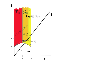
Figure 1: Fundamental domains for $\Gamma$ and $\Gamma_{\mathbb{Z}}$, with illustration of how $\mathbf{c}(T_{1})\left(R_{\frac{\pi}{2}}^{2}\right))$ rotates the subset $\mathscr{F}(\mathscr{G})\cap\mathbb{H}^{2}$ of $\mathscr{F}_{\mathbb{R}}(\mathscr{G}_{\mathbb{R}})$ into the other half of $\mathscr{F}_{\mathbb{R}}(\mathscr{G}_{\mathbb{R}})$.

We note for possible future reference that $\mathscr{F}_{\mathbb{R}}(\mathscr{G}_{\mathbb{R}})$ is the normal geodesic projection of the union of $\mathscr{F}(\mathscr{G})$ and one translate $\mathbf{c}(T_{1})\left(R_{\frac{\pi}{2}}^{2}\right)\mathscr{F}(\mathscr{G})$ of $\mathscr{F}(\mathscr{G})$. This relation between the fundamental domains is connected to the one given in Proposition 6.2, though neither relation implies the other, in general. In Figure 1, we have indicated by means of a “right-angle” symbol at the point $1+\sqrt{2}\mathbf{j}$ that the geodesic $\mathbb{H}^{1}(1+\sqrt{2}\mathbf{j},1+\mathbf{i}+\mathbf{j})$ is a geodesic normal to $\mathbb{H}^{2}_{\mathbf{j}}$. It would take us to far afield of our main purpose to define the concept of normal geodesic projection precisely, so for the moment we restrict ourselves to mentioning that this relation between $\mathscr{F}(\mathscr{G})$ and $\mathscr{F}_{\mathbb{R}}(\mathscr{G}_{\mathbb{R}})$ may be of some use in relating spectral expansions in the complex case to spectral expansions in the real case.

7 Spectral Zeta Functions

This section discusses a potential application of the results of the paper and indicates a future line of investigation building on this work. Jorgenson and Lang, in works such as [JL01], [JL06] (see the introduction to the latter work especially), and [JL], have laid out and begun to pursue an ambitious program of using heat kernel analysis to associate additive spectral zeta functions to quotients of symmetric spaces. When completed, this theory would subsume the basic theory of the Riemann zeta function and Selberg zeta function (among others), and clarify the relationship between the zeta functions arising at different geometric levels. The main component of the program is obtaining a theta inversion formula.

In [JL06], which carries out the derivation of the theta inversion formula for the special case of

$$X=\Gamma\backslash G/K=\mathrm{SL}_{2}(\mathbb{Z}[\mathbf{i}])\backslash\mathrm{SL}_{2}(\mathbb{C})/\mathrm{SU}(2,\mathbb{C}),\vspace{0.3cm}$$

the authors compute the regularized trace of an integral operator on functions on $X$. The kernel of the integral operator is $\mathbf{K}_{t,X}(z,w)$, the heat kernel on $X$. The trace of such an integral operator is defined to be the integral on the diagonal

$$\int_{X}\mathbf{K}_{t,X}(z,z)\,\mathrm{d}z.\vspace{0.3cm}$$

Although this integral is infinite, because of the cusp of $X$, the integrals over sets $X_{Y}$ approximating by covering $X$ only up to some fixed finite “distance” in the cusp are finite and diverge logarithmically in $Y$. That is,

(7.1) $$\lim_{Y\rightarrow\infty}\int_{X_{Y}}\mathbf{K}_{t,X}(z,z)\,\mathrm{d}z-c_{1}(t)\log Y\;\text{exists as a $\mathbb{C}$-valued function of $t$.}\vspace{0.3cm}$$

where $c_{1}(t)$ is a factor, constant in $Y$, and determined in [JL06]. For the purposes of such an integration, we can replace $X$ with a suitable fundamental domain $\mathscr{F}$. The fundamental domain $\mathscr{F}$ is an analytic model of $X$ in its universal covering space $\mathbb{H}^{3}$–see §3, below, for a precise definition of fundamental domain. Similarly, we replace the truncation $X_{Y}$ of $X$ with a matching truncation $\mathscr{F}_{Y}$ of $\mathscr{F}$.

To obtain the theta inversion formula, the limit of (7.1) is computed in two ways. One computation is from the expression of the heat kernel as the periodized heat kernel on the universal covering space $\mathbb{H}^{3}$. This method of computing the limit in (7.1) yields

(7.2) $$e^{-2t}(4t)^{-\frac{1}{2}}\Theta^{\rm NC}(1/t)+\Theta^{\rm Cus}(1/t).\vspace{0.3cm}$$

In (7.2), $\Theta^{\rm NC}(1/t)$, the inverted theta series, is defined in terms of invariants of certain $\Gamma$-conjugacy classes in $\Gamma$, while $\Theta^{\rm Cus}(1/t)$, the inverted theta integral, is a sum of products composed of special values of $\zeta_{\mathbb{Q}(\mathbf{i})}$, constants similar to Euler’s $\gamma$, and single integrals whose Gauss transforms are exact. (We refer to §XIV.7, of [JL06], for exact definitions of $\Theta^{\rm NC}(1/t)$, $\Theta^{\rm Cus}(1/t)$ and the other terms in the theta relation.) The other method of computing the limit in (7.1) is from the expansion of $\mathbf{K}_{t,X}(z,z)\,\mathrm{d}z$ in terms of the spectrum of the Laplacian $\mathbf{\Delta}_{X}$. This second method of computing the limit of (7.1) yields

(7.3) $$\theta_{\rm Cus}(t)+1+\theta_{\rm Eis}(t),\vspace{0.3cm}$$

where $\theta_{\rm Cus}(t)$ is the theta series $\sum_{j=1}^{\infty}e^{-\lambda_{j}t}$ and $\lambda_{j}$ are the eigenvalues of $\mathbf{\Delta}_{X}$, and $\theta_{\rm Eis}(t)$ is what remains as the limit of the integral of the convolution of $\mathbf{K}_{t,X}(z,w)$ with certain Eisenstein series, once the term $c_{1}(t)\log(Y)$ has been subtracted. Setting equal the two expressions, (7.2) and (7.3), for the same limit (7.1), we obtain the theta inversion formula for $X$,

(7.4) $$e^{-2t}(4t)^{-\frac{1}{2}}\Theta^{\rm NC}(1/t)+\Theta^{\rm Cus}(1/t)=\theta_{\rm Cus}(t)+1+\theta_{\rm Eis}(t).\vspace{0.3cm}$$

Next, note that there is an infinite sequence of arithmetic quotients

$$X_{n}=\mathrm{SL}_{n}(\mathbb{Z}[\mathbf{i}])\backslash\mathrm{SL}_{n}(\mathbb{C})/\mathrm{SU}(n),\;n>1,\vspace{0.3cm}$$

having $X=X_{2}$ as its first nontrivial member. Generalizations of (7.4) to $X_{n}$ for $n>2$ are discussed in [JL]. In order to obtain exact formulas analogous to (7.4), we would have to integrate over a fundamental domain, rather than over an appoximating Siegel set, which is a more common analytic model in the literature.

In the present work, we initiate an extension of the Jorgenson-Lang project to the sequence of arithmetic quotients

(7.5) $$\mathrm{SO}_{n}(\mathbb{Z}[\mathbf{i}])\backslash\mathrm{SO}_{n}(\mathbb{C})/\mathrm{SO}(n)\vspace{0.3cm}$$

and related arithmetic quotients of real forms of the symmetric spaces. The main results of the present paper are restricted to the group theory (Propositions 2.8 and 5.5) and fundamental domains (Propositions 4.4 and 6.2) in the first case of $n=2$. Nevertheless, some of the intermediate results are couched in a more general terminology and notation, with a view towards building upwards from the case $n=2$, to the case of a general $n$. Thus, our project includes a natural extension and generalization of Grenier’s work in [Gre88] and [Gre93] to a different sequence of symmetric spaces.

The identification

$$\mathrm{SL}_{2}(\mathbb{C})/\{\pm I\}\stackrel{{\scriptstyle\cong}}{{\longrightarrow}}\mathrm{SO}_{3}(\mathbb{C}),\vspace{0.3cm}$$

allows us to view the theta inversion relation (conjecturally) associated with the case $n=2$ in (7.5) as a theta inversion relation associated with a quotient of $\mathrm{SL}_{2}(\mathbb{C})/K$ by an arithmetic subgroup different from, but still commensurable, the “standard” arithmetic subgroup $\mathrm{SL}_{2}(\mathbb{Z}[\mathbf{i}])$. The results of this paper will, it is hoped, enable future investigations to apply the machinery developed in [JL06] to this “nonstandard” arithmetic subgroup $\mathbf{c}^{-1}(\mathrm{SO}_{3}(\mathbb{Z}[\mathbf{i}]))$ of $\mathrm{SL}_{2}(\mathbb{C})$ to obtain the corresponding theta function.

Bibliography

[BFZ02]
Martine Babillot, Renato Feres, and Abdelghani Zeghib.
Rigidité, groupe fondamental et dynamique, volume 13 of Panoramas et Synthèses [Panoramas and Syntheses].
Société Mathématique de France, Paris, 2002.
[Bre]
Eliot Brenner.
A fundamental domain of ford type for some integer subgroups of
orthogonal groups.
Preprint, arXiv:math.NT/0605012.
[Bre05]
Eliot Brenner.
Grenier domains for arithmetic domains groups and associated
tilings.
PhD thesis, Yale University, 2005.
[BS]
Eliot Brenner and Florin Spinu.
Selberg Zeta function for commensurable Kleinian groups.
To Appear.
[CHJT98]
Sultan Catto, Jonathan Huntley, Jay Jorgenson, and David Tepper.
On an analogue of Selberg’s eigenvalue conjecture for .
Proc. Amer. Math. Soc., 126(12):3455–3459, 1998.
[EGM98]
J. Elstrodt, F. Grunewald, and J. Mennicke.
Groups acting on hyperbolic space.
Springer Monographs in Mathematics. Springer-Verlag, Berlin, 1998.
[Fri05]
Joshua S. Friedman.
The Selberg trace formula and Selberg zeta-function for cofinite
Kleinian groups with finite-dimensional unitary representations.
Math. Z., 250(4):939–965, 2005.
[Gre88]
Douglas Grenier.
Fundamental domains for the general linear group.
Pacific J. Math., 132(2):293–317, 1988.
[Gre93]
Douglas Grenier.
On the shape of fundamental domains in .
Pacific J. Math., 160(1):53–66, 1993.
[Iwa95]
Henryk Iwaniec.
Introduction to the spectral theory of automorphic forms.
Biblioteca de la Revista Matemática Iberoamericana. [Library of the
Revista Matemática Iberoamericana]. Revista Matemática Iberoamericana,
Madrid, 1995.
[JL]
Jay Jorgenson and Serge Lang.
Heat Eisenstein Series on .
Springer Monographs in Mathematics. Springer-Verlag, New York.
To appear.
[JL01]
Jay Jorgenson and Serge Lang.
Spherical inversion on .
Springer Monographs in Mathematics. Springer-Verlag, New York, 2001.
[JL06]
Jay Jorgenson and Serge Lang.
Theta inversion on .
Springer Monographs in Mathematics. Springer-Verlag, New York, 2006.
[Lan76]
Serge Lang.
Introduction to modular forms.
Springer-Verlag, Berlin, 1976.
Grundlehren der mathematischen Wissenschaften, No. 222.
[SS]
Peter Sarnak and Andreas Strömbergsson.
Minima of epstein’s zeta function and heights of flat tori.
preprint.
[Vul04]
L. Ya. Vulakh.
Units in some families of algebraic number fields.
Trans. Amer. Math. Soc., 356(6):2325–2348 (electronic), 2004.
[VZ82]
A. B. Venkov and P. G. Zograf.
Analogues of Artin’s factorization formulas in the spectral theory
of automorphic functions associated with induced representations of
Fuchsian groups.
Izv. Akad. Nauk SSSR Ser. Mat., 46(6):1150–1158, 1343, 1982.
[Yasa]
Dan Yasaki.
Explicit reduction theory for SU(2,1;[]),
arXiv:math.NT/0601071.
[Yasb]
Dan Yasaki.
On the existence of spines for -rank 1 groups,
arXiv:math.NT/0601073.