Abstract

A fundamental domain of Ford type for some subgroups of orthogonal groups

April 2006

We initiate a study of the spectral theory of the locally symmetric space $X=\Gamma\backslash G/K$, where $G=\mathrm{SO}_{3}(\mathbb{C})$, $\Gamma=\mathrm{SO}_{3}(\mathbb{Z}[\mathbf{i}])$, $K=\mathrm{SO}(3)$. We write down explicit equations defining a fundamental domain for the action of $\Gamma$ on $G/K$. The fundamental domain is well-adapted for studying the theory of $\Gamma$-invariant functions on $G/K$. We write down equations defining a fundamental domain for the subgroup $\Gamma_{\mathbb{Z}}=\mathrm{SO}(2,1)_{\mathbb{Z}}$ of $\Gamma$ acting on the symmetric space $G_{\mathbb{R}}/K_{\mathbb{R}}$, where $G_{\mathbb{R}}$ is the split real form $\mathrm{SO}(2,1)$ of $G$ and $K_{\mathbb{R}}$ is its maximal compact subgroup $\mathrm{SO}(2)$. We formulate a simple geometric relation between the fundamental domains of $\Gamma$ and $\Gamma_{\mathbb{Z}}$ so described. We then use the previous results compute the covolumes of of the lattices $\Gamma$ and $\Gamma_{\mathbb{Z}}$ in $G$ and $G_{\mathbb{R}}$.

A fundamental domain of Ford type for some subgroups of orthogonal groups

A Preprint

by

Eliot Brenner

Center for Advanced Studies in Mathematics

at Ben Gurion University

May 2006

ACKNOWLEDGMENTS

The Institute for the Advanced Study of Mathematics at Ben-Gurion University provided support and a pleasant and stimulating working environment during the writing of this memoir. Additionally, the author thanks Mr. Tony Petrello for financial assistance.

Chapter I Fundamental Domain

1 Representation of $\mathrm{SO}_{3}(\mathbb{Z}[\mathbf{i}])$ as a lattice in $\mathrm{SL}_{2}(\mathbb{C})$

We begin by establishing some basic notational conventions.

Let $n$ be a positive integer and $\mathfrak{o}$ a ring. We will use $\mathrm{Mat}_{n}(\mathfrak{o})$ to denote the set of all$n$-by-$n$ square matrices with coefficients in $\mathfrak{o}$. We reserve use the Greek letters $\alpha$, and so on, for the elements of $\mathrm{Mat}_{n}(\mathfrak{o})$, and the roman letters $a,b,c,d$ and so on, for the entries of the matrices. We will denote scalar mutliplication on $\mathrm{Mat}_{n}(\mathfrak{o})$ by simple juxtaposition. Thus, if $\mathfrak{o}=\mathbb{Z}[\mathbf{i}]$, $\ell\in\mathbb{Z}[\mathbf{i}]$ and $\alpha\in\mathrm{Mat}_{2}(\mathbb{Z}[\mathbf{i}])$, then

$$\alpha=\begin{pmatrix}a&b\\ c&d\end{pmatrix}\;\text{implies}\;\ell\alpha=\begin{pmatrix}\ell a&\ell b\\ \ell c&\ell d\end{pmatrix}.\vspace{0.3cm}$$

The letters $p,q,r,s$ will be reserved to denote a quadruple of elements of $\mathfrak{o}$ such that $ps-rq=1$. In what follows, we normally have $\mathfrak{o}=\mathbb{Z}[\mathbf{i}]$, whenever $\alpha$ is written with entries $p$ through $s$. Therefore,

$$\alpha=\begin{pmatrix}p&q\\ r&s\end{pmatrix}\in\mathrm{SL}_{2}(\mathbb{Z}[\mathbf{i}]),\vspace{0.3cm}$$

unless stated otherwise.

1.1 Realization of $\mathrm{SO}_{3}(\mathbb{Z}[\mathbf{i}])$ as a group of fractional linear transformations

We will denote a conjugation action of a group on a space $V$ by $\mathbf{c}_{V}$, when the context makes clear what this action is. For example, if $H$ is a linear Lie group and $\mathfrak{h}$ the Lie algebra of $H$, then we have

$$\mathbf{c}_{\mathfrak{h}}(h)X=hXh^{-1},\quad\text{for all}\;h\in H,\;X\in\mathfrak{h}.\vspace{0.3cm}$$

Note that the morphism $\mathbf{c}_{\mathfrak{h}}(h)$ is the image under the Lie functor of the usual conjugation $\mathbf{c}_{H}(h)$ on the group level. Using $\mathrm{SL}(V)$ to denote the group of unimodular transformations of a vector space $V$, it is easy to see that

(1.1.1) $$\mathbf{c}_{\mathfrak{h}}:H\rightarrow SL(\mathfrak{h})\;\text{is a Lie group morphism}.\vspace{0.3cm}$$

Henceforth, whenever $H$ is a group acting on a Lie algebra $\mathfrak{h}$ by conjugation, we will omit the subscript $\mathfrak{h}$. Thus, we define

$$\mathbf{c}:=\mathbf{c}_{\mathfrak{h}},\vspace{0.3cm}$$

when we are in the situation of (1.1.1).

Throughout (except in a few sections where it is prominently noted otherwise), we will use the notation $G=\mathrm{SO}_{3}(\mathbb{C})$, $\Gamma=\mathrm{SO}_{3}(\mathbb{Z}[\mathbf{i}])$. We use $B$ to denote the half-trace form on $\mathfrak{sl}_{2}(\mathbb{C})$, the Lie algebra of traceless $2$-by-$2$ matrices. That is,

$$B(X,Y)=\frac{1}{2}\mathrm{Tr}(XY).\vspace{0.3cm}$$

We use the notation $\beta^{\prime}=\{X^{\prime}_{1},X^{\prime}_{2},Y^{\prime}\}$ for the “standard” basis of $\mathfrak{sl}_{2}(\mathbb{C})$, where

(1.1.2) $$\begin{gathered}X_{1}^{\prime}=\begin{pmatrix}0&1\\ 0&0\end{pmatrix},\qquad X_{2}^{\prime}=\begin{pmatrix}0&0\\ 1&0\end{pmatrix},\\ \text{and}\quad Y^{\prime}=\begin{pmatrix}1&0\\ 0&-1\end{pmatrix}\end{gathered}\vspace{0.3cm}$$

The following properties of $B$ are verified either immediately from the definition or by straightforward calculations.

• $B$ is nondegenerate.

• Setting

  (1.1.3) $$\begin{gathered}X_{1}=X_{1}^{\prime}+X_{2}^{\prime},\qquad X_{2}=\mathbf{i}(X_{1}^{\prime}-X_{2}^{\prime}),\\ \text{and}\quad Y=Y^{\prime},\end{gathered}\vspace{0.3cm}$$

  we obtain an orthonormal basis $\beta=\{X_{1},X_{2},Y\}$, with respect to the bilinear form $B$.

• $B$ is invariant under the conjugation action of $\mathrm{SL}_{2}(\mathbb{C})$, meaning that

  $$B(X,Y)=B(\mathbf{c}(g)Z,\mathbf{c}(g)W),\quad\text{for all}\;Z,W\in\mathfrak{sl}_{2}(\mathbb{C}),\,g\in\mathrm{SL}_{2}(\mathbb{C}).\vspace{0.3cm}$$

By B3, $\mathbf{c}$ is a morphism of $\mathrm{SL}_{2}(\mathbb{C})$ into $G$. The content of part (a) of Proposition 1.1.1 below is that the morphism $\mathbf{c}$ just described is an epimorphism.

As a consequence of B1 and B2, we have that

(1.1.4) $$B(x^{1}_{1}X_{1}+x^{1}_{2}X_{2}+y^{1}Y,x^{2}_{1}X_{1}+x^{2}_{2}X_{2}+y^{2}Y)=x^{1}_{1}x^{2}_{1}+x^{1}_{2}x^{2}_{2}+y^{1}y^{2},\;x^{i}_{j},y\in\mathbb{C}.\vspace{0.3cm}$$

For any bilinear form $B$ on a vector space $V$, we use $\mathrm{O}(B)$ to denote the group of linear transformations of $V$ preserving $B$, and we use $\mathrm{SO}(B)$ to denote the unimodular subgroup of $\mathrm{O}(B)$. If $B$ is as in (1.1.4), then the isomorphism,

(1.1.5) $$\mathrm{SO}(B)\cong G,\vspace{0.3cm}$$

induced by the identification of the vector space $\mathfrak{sl}_{2}(\mathbb{C})$ with $\mathbb{C}\langle X_{1},X_{2},Y\rangle$, puts a system of coordinates on $G$. Part (b) of Proposition 1.1.1, below, will describe the epimorphism $\mathbf{c}:\mathrm{SL}_{2}(\mathbb{C})\rightarrow G$ in terms of these coordinates.

         Proposition 1.1.1.

With $G$, $\mathbf{c}$ as above, we have

• The map $\mathbf{c}$ induces an isomorphism

  $$\mathrm{SL}_{2}(\mathbb{C})/\{\pm I\}\stackrel{{\scriptstyle\cong}}{{\longrightarrow}}G\vspace{0.3cm}$$

  of Lie groups.

• Relative to the standard coordinates on $\mathrm{SL}_{2}(\mathbb{C})$ and the coordinates on $G$ induced from the orthonormal basis $\beta$ of $\mathfrak{sl}_{2}(\mathbb{C})$, as defined in (1.1.3), the epimorphism $\mathbf{c}:\mathrm{SL}_{2}(\mathbb{C})\rightarrow G$ has the following coordinate expression.

  (1.1.6) $$\mathbf{c}\left(\begin{pmatrix}a&b\\ c&d\end{pmatrix}\right)=\begin{pmatrix}\frac{a^{2}-c^{2}+d^{2}-b^{2}}{2}&\frac{\mathbf{i}(a^{2}-c^{2}+b^{2}-d^{2})}{2}&cd-ab\vspace*{0,2cm}\\ \frac{\mathbf{i}(b^{2}+d^{2}-a^{2}-c^{2})}{2}&\frac{a^{2}+c^{2}+b^{2}+d^{2}}{2}&\mathbf{i}(ab+cd)\vspace*{0.2cm}\\ -ac+bd&\mathbf{i}(ac+bd)&ad+bc\end{pmatrix}.\vspace{0.3cm}$$

Before giving the proof of the Proposition, we establish some further notational conventions regarding conjugation mappings. Whenever a matrix group $H$ has a conjugation action $\mathbf{c}_{V}$ on a finite dimensional vector space $V$ over a field $F$, each basis $\beta$ of $V$ naturally induces a morphism

(1.1.7) $$\mathbf{c}_{V,\beta}:H\rightarrow\mathrm{GL}_{N}(F),\;\text{where}\;N=\dim V.\vspace{0.3cm}$$

Let $\beta,\beta^{\prime}$ be two bases of $V$. Write $\alpha^{\beta\mapsto\beta^{\prime}}$ for the change-of-basis matrix from $\beta$ to $\beta^{\prime}$. That is, if $\beta$, $\beta^{\prime}$ are written as $N$-entry row-vectors, then

(1.1.8) $$\beta\alpha^{\beta\mapsto\beta^{\prime}}=\beta^{\prime}.\vspace{0.3cm}$$

Then elementary linear algebra tells us that

(1.1.9) $$\mathbf{c}_{V,\beta} = \mathbf{c}_{\mathrm{GL}_{N}(F)}\left(\left(\alpha^{\beta\mapsto\beta^{\prime}}\right)^{-1}\right)\mathbf{c}_{V,\beta^{\prime}}$$

$$= \mathbf{c}_{\mathrm{GL}_{N}(F)}\left(\alpha^{\beta^{\prime}\mapsto\beta}\right)\mathbf{c}_{V,\beta^{\prime}}.$$

Assuming that $c_{V}$ is injective, and writing $c_{V}^{-1}$ for the left-inverse of $c_{V}$, we calculate from (1.1.9) that

(1.1.10) $$\mathbf{c}_{V,\beta}\mathbf{c}_{V,\beta^{\prime}}^{-1}\in\mathrm{Aut}(\mathrm{GL}_{N}(F))\;\text{is given by}\;\mathbf{c}_{\mathrm{GL}_{N}(F)}\left(\alpha^{\beta\mapsto\beta^{\prime}}\right).\vspace{0.3cm}$$

In keeping with the practice established after (1.1.1), we will omit the subscript $\mathfrak{h}$ when $H$ is a Lie group acting on its Lie algebra by conjugation. Thus, for any basis $\beta$ of $\mathfrak{h}$,

$$\mathbf{c}_{\beta}:=\mathbf{c}_{\mathfrak{h},\beta}.\vspace{0.3cm}$$

Further, except in situations such as the proofs of Proposition 1.1.1 and 3.1.3 below, where we are dealing with $\mathbf{c}_{\beta}$ for different bases $\beta$ of $\mathfrak{h}$ at the same time, we will fix a single basis $\beta$ for $\mathfrak{h}$ and blur the distinction between $\mathbf{c}$ and $\mathbf{c}_{\beta}$. For example, in this chapter, whenever $H=\mathrm{SL}_{2}(\mathbb{C})$ and $V=\mathrm{Lie}(H)$, we will write $\mathbf{c}$ to denote both the “abstract” morphism $\mathbf{c}$ of $H$ into $\mathrm{Aut}(V)$ and the linear morphism $\mathbf{c}_{\beta}$ of $H$ into $\mathrm{GL}_{3}(\mathbb{C})$, where $\beta$ is the orthonormal basis for $\mathrm{Lie}(H)$ defined in (1.1.3). Whenever the linear morphism into $\mathrm{GL}_{3}(\mathbb{C})$ is induced by a basis $\beta^{\prime}\neq\beta$, the notation $\mathbf{c}_{\beta^{\prime}}$ will be used.

Proof of Proposition 1.1.1. For (a), it is clear that the kernel of $\mathbf{c}$ is the center of $\mathrm{SL}_{2}(\mathbb{C})$, which equals $\{\pm I\}$. The surjectivity of $\mathbf{c}$ follows from a comparison of the dimensions of $\mathrm{SL}_{2}(\mathbb{C})$ and $G$ (both have complex dimension $3$), and from the well-known fact that $G$ is connected.

Let $h\in\mathrm{SL}_{2}(\mathbb{C})$, so that

$$h=\begin{pmatrix}a&b\\ c&d\end{pmatrix},\quad\text{with}\;ad-bc=1.\vspace{0.3cm}$$

Recall the basis $\beta^{\prime}=\{X_{1}^{\prime},X_{2}^{\prime},Y^{\prime}\}$ for $\mathrm{Lie}(\mathrm{SL}_{2}(\mathbb{C}))$. A routine calculation using (1.1.2) shows that we have

(1.1.11) $$\mathbf{c}_{\beta^{\prime}}(h)=\begin{pmatrix}a^{2}&-b^{2}&-2ab\\ -c^{2}&d^{2}&2cd\\ -ac&bd&ad+bc\end{pmatrix}.\vspace{0.3cm}$$

Let $\alpha^{\beta\mapsto\beta^{\prime}}$ be the change-of-basis matrix, satisfying relation (1.1.8). As a consequence of the the relations (1.1.3), we obtain

(1.1.12) $$(\alpha^{\beta\mapsto\beta^{\prime}})^{-1}=\begin{pmatrix}1&\mathbf{i}&0\\ 1&-\mathbf{i}&0\\ 0&0&1\end{pmatrix}.\vspace{0.3cm}$$

Using (1.1.9), (1.1.12), and (1.1.11) we obtain

$$\mathbf{c}(h):=\mathbf{c}_{\beta}(h)=\begin{pmatrix}\frac{a^{2}-c^{2}+d^{2}-b^{2}}{2}&\frac{\mathbf{i}(a^{2}-c^{2}+b^{2}-d^{2})}{2}&cd-ab\vspace*{0.2cm}\\ \frac{\mathbf{i}(b^{2}+d^{2}-a^{2}-c^{2})}{2}&\frac{a^{2}+c^{2}+b^{2}+d^{2}}{2}&\mathbf{i}(ab+cd)\vspace*{0.2cm}\\ -ac+bd&\mathbf{i}(ac+bd)&ad+bc\end{pmatrix}.\vspace{0.3cm}$$

This gives part (b) of the proposition. ∎

Whenever $G_{1}\subseteq\mathrm{GL}_{N_{1}}(F)$ and $G_{2}\subseteq\mathrm{GL}_{N_{2}}(F)$ are linear groups and $\varphi$ is a morphism expressed by a formula involving only polynomial functions of the entries, $\varphi$ may be extended to a rational map

$$\tilde{\varphi}:\mathrm{M}(_{,}N_{1})(F)\rightarrow\mathrm{M}(_{,}N_{2})(F).\vspace{0.3cm}$$

For example, since all the entries in (1.1.6) are polynomials in the entries of the matrix in $\mathrm{SL}_{2}(\mathbb{C})$, we may extend $\mathbf{c}$ to a map

(1.1.13) $$\tilde{\mathbf{c}}:\mathrm{Mat}_{2}(\mathbb{C})\rightarrow\mathrm{Mat}_{3}(\mathbb{C}).\vspace{0.3cm}$$

We note some properties of $\tilde{\mathbf{c}}$ that will be useful later. Let $\ell$ denote a complex number and $\alpha$ an arbitrary 2-by-2 matrix.

(1.1.14) If $$\tilde{\mathbf{c}}(\alpha) \ell^{2}\in\mathbb{Z}[\mathbf{i}] \tilde{\mathbf{c}}(\ell\alpha)$$ has integral entries and then has integral entries.

We deduce (1.1.14) by observing that the entries of $\tilde{\mathbf{c}}(\alpha)$ are homogeneous polynomials of degree $2$ in the entries of $\alpha$. As an immediate corollary of (1.1.14), one has

(1.1.15) If $$\ell^{2}\in\mathbb{Z}[\mathbf{i}]^{*} \tilde{\mathbf{c}}(\alpha) \tilde{\mathbf{c}}(\ell\alpha)$$, then has integral entries if and only if has integral entries.

We now wish to describe the inverse image $\mathbf{c}^{-1}(\Gamma)$ as a subset of $\mathrm{SL}_{2}(\mathbb{C})/\{\pm I\}$ with respect to the standard coordinates of $\mathrm{SL}_{2}(\mathbb{C})$. According to Proposition 1.1.1, this amounts to describing the quadruples

(1.1.16) $$(a,b,c,d)\in\mathbb{C}^{4},\;\text{with $ad-bc=1$, and the entries of the right-side of \eqref{eqn:imagematrixconj} integers.}\vspace{0.3cm}$$

Describing the quadruples meeting conditions (1.1.16) will be the subject of the remainder of this section and the next, culminating in the proof of Proposition 1.1.9.

Conventions regarding multiplicative structure of $\mathbb{Z}[\mathbf{i}]$. Before stating the proposition, we establish certain conventions we will use when dealing with the multiplicative properties of the Euclidean ring $\mathbb{Z}[\mathbf{i}]$. First, it is well-known that $\mathbb{Z}[\mathbf{i}]$ is a Euclidean, hence principal, ring. That $\mathbb{Z}[\mathbf{i}]$ is principal means that all ideals $\mathscr{I}$ of $\mathbb{Z}[\mathbf{i}]$ are generated by a single element $m\in\mathbb{Z}[\mathbf{i}]$, so that every $\mathscr{I}$ is of the form $(m)$. However, there is an unavoidable ambiguity in the choice of generators caused by the presence in $\mathbb{Z}[\mathbf{i}]$ of four units, $\mathbf{i}^{j}$, for $j\in\{0,\ldots,3\}$, in $\mathbb{Z}[\mathbf{i}]$. We will adopt the following convention to sidestep the ambiguity caused by the group of units.

         Definition 1.1.2.

We refer to the following subset of $\mathbb{C}^{\times}$ as the standard subset

(1.1.17) $$\{z\in\mathbb{C}^{\times}\;|\;\mathrm{Re}(z)>0,\,\mathrm{Im}(z)\geq 0\}.\vspace{0.3cm}$$

That is, the standard subset of $\mathbb{C}^{\times}$ is the union of the interior of the first quadrant and the positive real axis. An element of $\mathbb{Z}[\mathbf{i}]$ in the standard subset will be referred to as a standard Gaussian integer, or more simply as a standard integer when the context is clear.

Because of the units in $\mathbb{Z}[\mathbf{i}]$, each nonzero ideal $\mathscr{I}$ of $\mathbb{Z}[\mathbf{i}]$ has precisely one generator which is a standard integer. Henceforth, we refer to generator of $\mathscr{I}$ which is a standard integer as the standard generator of $\mathscr{I}$. Unless otherwise stated, whenever we write $\mathscr{I}=(m)$, to indicate the ideal $\mathscr{I}$ generated by an $m\in\mathbb{Z}[\mathbf{i}]$, it will be understood that $m$ is standard. Conversely, whenever we write an ideal $\mathscr{I}$ in the form $(m)$, it will be understood that $m$ is the standard generator of $\mathscr{I}$. Thus, for example, since $(1-\mathbf{i})=\mathbf{i}^{3}(1+\mathbf{i})$ with $1+\mathbf{i}$ standard, we write $\mathscr{I}=:(1-\mathbf{i})\mathbb{Z}[\mathbf{i}]$, defined as the ideal of Gaussian integers divisible by $1-\mathbf{i}$, in the form $\mathscr{I}=(1+\mathbf{i})$.

Similar comments apply to Gaussian primes, factorization, and greatest common divisor in $\mathbb{Z}[\mathbf{i}]$. By a “prime in $\mathbb{Z}[\mathbf{i}]$”, we will always mean a standard prime. By “prime factorization” in $\mathbb{Z}[\mathbf{i}]$ we will always mean factorization into a product of standard primes, multiplied by the appropriate unit factor. Note that the convention regarding standard primes uniquely determines the unit factor in a prime factorization. For example, since

$$2=\mathbf{i}^{3}(1+\mathbf{i})^{2}\vspace{0.3cm}$$

and $(1+\mathbf{i})^{3}$ is standard, the above expression is the standard factorization of the Gaussian integer $2$, and $\mathbf{i}^{3}$ is uniquely determined as the standard unit factor in the prime factorization of $2\in\mathbb{Z}[\mathbf{i}]$.

         Definition 1.1.3.

For $x,\,y\in\mathbb{Z}[\mathbf{i}]$, consider $(x,y)\mathbb{Z}[\mathbf{i}]$, the ideal generated by $x$ and $y$. Define

$$\text{\boldmath$\mathrm{GCD}(x,y)$\unboldmath to be the unique}\;m\in\mathbb{Z}[\mathbf{i}]\;\text{such that $m$ is standard and}\;(m)=(x,y)\mathbb{Z}[\mathbf{i}].\vspace{0.3cm}$$

We will use the following three basic properties of $\mathrm{GCD}(x,y)$. In each case, the proof is the same as for the corresponding properties of the greatest common divisor for the rational integers. Let $x,\,y,\,z\in\mathbb{Z}[\mathbf{i}]$. Then we have

• $\mathrm{GCD}(x,y)|x$,

• $\mathrm{GCD}\left(\frac{x}{\mathrm{GCD}(x,y)},\frac{y}{\mathrm{GCD}(x,y)}\right)=1$,

• There exist $z,w\in\mathbb{Z}[\mathbf{i}]$ such that $xz-yw=\mathrm{GCD}(x,y)$.

By convention, unless stated otherwise, the “trivial ideal” $\mathbb{Z}[\mathbf{i}]$ will be understood to belong to the set of ideals of $\mathbb{Z}[\mathbf{i}]$. The standard generator of the trivial ideal $\mathbb{Z}[\mathbf{i}]$ is, of course, $1$.

To facilitate the statement of Proposition 1.1.9, we estblish the following conventions. First, we use $\omega_{8}$ to denote the unique primitive eighth root of unity in the standard set of $\mathbb{C}^{\times}$. Observe that

(1.1.18) $$\omega_{8}=\frac{\sqrt{2}}{2}(1+\mathbf{i}),\quad\text{and}\quad\omega_{8}^{2}=\mathbf{i}.\vspace{0.3cm}$$

The $\mathrm{SL}_{2}(\mathbb{Z}[\mathbf{i}])$-space $\mathrm{M}_{2}^{\mathrm{N}}$.

         Definition 1.1.4.

For $N\in\mathbb{Z}[\mathbf{i}]$, $\mathrm{M}_{2}^{\mathrm{N}}\;$will the subset of $\mathrm{Mat}_{2}(\mathbb{Z}[\mathbf{i}])$ consisting of the elements with determinant $N$. Since the group $\mathrm{SL}_{2}(\mathbb{Z}[\mathbf{i}])$ acts on $\mathrm{M}_{2}^{\mathrm{N}}$ by multiplication on the left, $\mathrm{M}_{2}^{\mathrm{N}}$ is a $\mathrm{SL}_{2}(\mathbb{Z}[\mathbf{i}])$-space.

It is not difficult to see that the action of $\mathrm{SL}_{2}(\mathbb{Z}[\mathbf{i}])$ on $\mathrm{M}_{2}^{\mathrm{N}}$ fails to be transitive, so $\mathrm{M}_{2}^{\mathrm{N}}$ is not a $\mathrm{SL}_{2}(\mathbb{Z}[\mathbf{i}])$-homogeneous space. The purpose of the subsequent definitions and results is to give a description of the orbit structure of the $\mathrm{SL}_{2}(\mathbb{Z}[\mathbf{i}])$-space $\mathrm{M}_{2}^{\mathrm{N}}$.

Let

(1.1.19) $$\Omega_{y}:=\text{a fixed set of representatives of $\mathbb{Z}[\mathbf{i}]/(y)$},\;\text{for all}\;y\in\mathbb{Z}[\mathbf{i}]\vspace{0.3cm}$$

It is clear that, for each $y\in\mathbb{Z}[\mathbf{i}]$, a number of possible $\Omega_{y}$ exist. For the general result, Proposition 1.1.7, below, the choice of $\Omega_{y}$ does not matter, and we leave it unspecified. However, in the specific applications of Proposition 1.1.7, where $y$ is always of the form $y=(1+\mathbf{i})^{n}$ for $n$ a positive integer, it will be essential to give an $\Omega_{y}$ explicitly, which we now do.

So let $n\in\mathbb{N}$, $n\geq 1$. In the definition of $\Omega_{(1+\mathbf{i})^{n}}$, we use the “ceiling” notation, defined as follows:

$$\lceil q\rceil\;=\text{smallest integer $\geq\frac{x}{y}$.}\vspace{0.3cm}$$

Now set

(1.1.20) $$\Omega_{(1+\mathbf{i})^{n}}=\left\{r+s\mathbf{i}\;\text{with $r,\,s\in\mathbb{Z}$, $0\leq r<2^{\lceil\frac{n}{2}\rceil}$, $0\leq s<2^{n-\lceil\frac{n}{2}\rceil}$}\right\}.\vspace{0.3cm}$$

The definition is justified by Lemma 1.1.5, below. In order not to interrupt the flow of paper, we delay the proof of Lemma 1.1.5 until the end of §1.1.

         Lemma 1.1.5.

For $n\geq 1$ an integer, let $\Omega_{(1+\mathbf{i})^{n}}$ be defined as (1.1.20). Then

$$\Omega_{(1+\mathbf{i})^{n}}\;\text{is a complete set of representatives of $\mathbb{Z}[\mathbf{i}]/\left((1+\mathbf{i})^{n}\right)$}\;\text{ for all $n$}.\vspace{0.3cm}$$

         Definition 1.1.6.

Let $N\in\mathbb{Z}[\mathbf{i}]$ be fixed, and for each $y\in\mathbb{Z}[\mathbf{i}]$ let $\Omega_{y}$ be as in (1.1.19). Define the matrix $\alpha^{\mathrm{N}}(m,x)\in\mathrm{M}_{2}^{\mathrm{N}}$ as follows,

(1.1.21) $$\alpha^{\mathrm{N}}(m,x)=\begin{pmatrix}m&x\\ 0&\frac{N}{m}\end{pmatrix},\;\text{for}\;m\in\mathbb{Z}[\mathbf{i}],\,m|N,\,x\in\Omega_{\frac{N}{m}}.\vspace{0.3cm}$$

It is trivial to verify that $\alpha^{\mathrm{N}}(m,x)$, as given by (1.1.21), indeed has determinant $N$, i.e. $\alpha^{\mathrm{N}}(m,x)\in\mathrm{M}_{2}^{\mathrm{N}}$. The point of Definition 1.1.6 is given by the following proposition.

         Proposition 1.1.7.

For $N\in\mathbb{Z}[\mathbf{i}]-\{0\}$, let $\mathrm{M}_{2}^{\mathrm{N}}$ be the $\mathrm{SL}_{2}(\mathbb{Z}[\mathbf{i}])$-space of matrices with entries in $\mathbb{Z}[\mathbf{i}]$ and determinant $N$. Define the matrices $\alpha^{\mathrm{N}}(m,x)$ as in (1.1.21). Then

(1.1.22) $$\mathrm{\mathrm{M}_{2}^{\mathrm{N}}}=\bigcup_{\left\{\stackrel{{\scriptstyle m\in\mathbb{Z}[\mathbf{i}]|\;m|N,}}{{\frac{N}{m}\;\text{standard}}}\right\}}\cdot\hskip 28.45274pt\bigcup_{x\in\Omega_{\frac{N}{m}}}\cdot\hskip 15.6491pt\mathrm{SL}_{2}(\mathbb{Z}[\mathbf{i}])\alpha^{\mathrm{N}}(m,x),\vspace{0.3cm}$$

and (1.1.22) gives the decomposition of the $\mathrm{SL}_{2}(\mathbb{Z}[\mathbf{i}])$-space $\mathrm{M}_{2}^{\mathrm{N}}$ into distinct $\mathrm{SL}_{2}(\mathbb{Z}[\mathbf{i}])$-orbits.

We delay the proof of Proposition 1.1.7 until the end of §1.1, and here restrict ourselves to some concerning the significance of Proposition 1.1.7. First, a statement equivalent to Proposition 1.1.7 is that an arbitrary $\alpha\in M_{2}^{\rm N}$ has a uniquely determined product decomposition of the form

(1.1.23) $$\alpha=\begin{pmatrix}a&b\\ c&d\end{pmatrix}=\begin{pmatrix}p&q\\ r&s\end{pmatrix}\begin{pmatrix}m&x\\ 0&\frac{N}{m}\end{pmatrix},\;\text{with}\,m\in\mathfrak{o},\;m|N,\;\frac{N}{m}\;\text{standard},\;x\in\Omega_{\frac{N}{m}},\,pr-qs=1.\vspace{0.3cm}$$

The uniqueness is derived from Proposition 1.1.7 as follows. The second matrix in the product of (1.1.23) is uniquely determined by the matrix decomposition because of the disjointness of the union in (1.1.22). The first matrix in the product appearing in (1.1.23) is therefore also uniquely determined.

The second remark is that Proposition 1.1.7 may be thought of as the Gaussian-integer version of the decomposition of elements of $\mathrm{Mat}_{2}(\mathbb{Z})$ of fixed determinant $N$, sometimes known as the Hecke decomposition. Occasionally we refer to (1.1.23) as the Gaussian Hecke decomposition, to distinguish it from this classical Hecke decomposition in the context of the rational integers. Readers familiar with the the proof of the classical Hecke decomposition may skip the proof of Proposition (1.1.7), since the proof is the same as that of the classical decomposition except for some care that has to be taken because of the presence of additional units in $\mathbb{Z}[\mathbf{i}]$. For the classical Hecke decomposition, see page 110, §VII.4, of [Lan76], which is the source of our notation for the Gaussian version.

Statement of the Main Result of §1. Let $\Xi$ be an arbitrary subset of $\mathrm{SL}_{2}(\mathbb{Z}[\mathbf{i}])$. Suppose, at first, that $\Xi$ is actually a subgroup of $\mathrm{SL}_{2}(\mathbb{Z}[\mathbf{i}])$. Since $\mathrm{SL}_{2}(\mathbb{Z}[\mathbf{i}])\alpha^{\mathrm{N}}(m,x)$ is an $\mathrm{SL}_{2}(\mathbb{Z}[\mathbf{i}])$-space, it is also a $\Xi$-space. For general, $\Xi$, however, the action of $\Xi$ on $\mathrm{SL}_{2}(\mathbb{Z}[\mathbf{i}])\alpha^{\rm N}(m,x)$ fails to be transitive, i.e., $\mathrm{SL}_{2}(\mathbb{Z}[\mathbf{i}])\alpha^{\mathrm{N}}(m,x)$ is not a $\Xi$-homogeneous space. We will now describe the orbit structure of $\mathrm{SL}_{2}(\mathbb{Z}[\mathbf{i}])\alpha^{\mathrm{N}}(m,x)$ for a specific subgroup $\Xi$. In order to make the description of the subgroup and some related subsets of $\mathrm{SL}_{2}(\mathbb{Z}[\mathbf{i}])$ easier, we introduce the epimorphism

$$\mathrm{red}_{1+\mathbf{i}}:\mathrm{SL}_{2}(\mathbb{Z}[\mathbf{i}])\rightarrow\mathrm{SL}_{2}(\mathbb{Z}[\mathbf{i}]/(1+\mathbf{i}))\vspace{0.3cm}$$

by inducing from the reduction map

$$\mathrm{red}_{1+\mathbf{i}}:\mathbb{Z}[\mathbf{i}]\rightarrow\mathbb{Z}[\mathbf{i}]/(1+\mathbf{i})\vspace{0.3cm}$$

That is, we “extend” $\mathrm{red}_{1+\mathbf{i}}$ from elements to matrices by setting

(1.1.24) $$\mathrm{red}_{1+\mathbf{i}}\left(\begin{pmatrix}p&q\\ r&s\end{pmatrix}\right)=\begin{pmatrix}\mathrm{red}_{1+\mathbf{i}}p&\mathrm{red}_{1+\mathbf{i}}q\\ \mathrm{red}_{1+\mathbf{i}}r&\mathrm{red}_{1+\mathbf{i}}s\end{pmatrix}.\vspace{0.3cm}$$

Since $\Omega_{1+\mathbf{i}}=\{0,1\}$, we may identify $\mathbb{Z}[\mathbf{i}]/(1+\mathbf{i})$ with $\{0,1\}$. Similarly to the convention with $p,q,r,s\in\mathbb{Z}[\mathbf{i}]$, we use $(\overline{p},\overline{q},\overline{r},\overline{s})$ to denote a quadruple of elements of $\mathbb{Z}[\mathbf{i}]/(1+\mathbf{i})$ such that

$$\overline{p}\hskip 1.42262pt\overline{s}-\overline{r}\hskip 1.42262pt\overline{q}=1.\vspace{0.3cm}$$

Here are two elements of $\mathrm{SL}_{2}(\mathbb{Z}[\mathbf{i}]/(1+\mathbf{i}))$ of particular interest.

(1.1.25) $$\overline{I}:=\begin{pmatrix}1&0\\ 0&1\end{pmatrix},\;\overline{S}:=\begin{pmatrix}0&1\\ 1&0\end{pmatrix}\in\mathrm{SL}_{2}(\mathbb{Z}[\mathbf{i}]/(1+\mathbf{i})).\vspace{0.3cm}$$

The notation in (1.1.25) is chosen to remind the reader that $\overline{I}=\mathrm{red}_{1+\mathbf{i}}(I)$ and $\overline{S}=\mathrm{red}_{1+\mathbf{i}}(S)$, where $I,\,S$ are the standard generators of $\mathrm{SL}_{2}(\mathbb{Z})$, as in §VI.1 of [JL06]. Since $\overline{S}^{2}=\overline{I}$, it is easy to see that $\{\overline{I},\overline{S}\}$ is a subgroup of $\mathrm{SL}_{2}(\mathbb{Z}[\mathbf{i}]/(1+\mathbf{i}))$. Now define

(1.1.26) $$\Xi_{12}=\mathrm{red}_{1+\mathbf{i}}^{-1}(\{\overline{I},\,\overline{S}\}).\vspace{0.3cm}$$

Since $\mathrm{red}_{1+\mathbf{i}}$ is a morphism, $\Xi_{12}$ is a subgroup of $\mathrm{SL}_{2}(\mathbb{Z}[\mathbf{i}])$.

Also, using the epimorphism $\mathrm{red}_{1+\mathbf{i}}$ we define the following subsets of $\mathrm{SL}_{2}(\mathbb{Z}[\mathbf{i}])$:

(1.1.27) $$\Xi_{1} = \mathrm{red}_{1+\mathbf{i}}^{-1}\left(\left\{\begin{pmatrix}0&1\\ 1&1\end{pmatrix},\,\begin{pmatrix}1&1\\ 0&1\end{pmatrix}\right\}\right),$$

$$\Xi_{2} = \mathrm{red}_{1+\mathbf{i}}^{-1}\left(\left\{\begin{pmatrix}1&1\\ 1&0\end{pmatrix},\,\begin{pmatrix}1&0\\ 1&1\end{pmatrix}\right\}\right).$$

(The subscripts on the $\Xi$ of (1.1.26) and (1.1.27) are chosen in order to remind the reader of the column in which zeros appear in the matrices of $\mathrm{red}_{1+\mathbf{i}}(\Xi)$.) Since $\mathrm{SL}_{2}(\mathbb{Z}[\mathbf{i}]/(1+\mathbf{i}))$ consists of the elements $\overline{I},\overline{S}$ and the four elements appearing on the right-hand side of (1.1.27), and $\mathrm{red}_{1+\mathbf{i}}$ is an epimorphism,

(1.1.28) $$\mathrm{SL}_{2}(\mathbb{Z}[\mathbf{i}])=\Xi_{1}\bigcup\cdot\hskip 9.24706pt\Xi_{2}\bigcup\cdot\hskip 9.24706pt\Xi_{12}.\vspace{0.3cm}$$

Unlike $\Xi_{12}$, the subsets $\Xi_{1}$ and $\Xi_{2}$ of $\mathrm{SL}_{2}(\mathbb{Z}[\mathbf{i}])$ are not subgroups. All three subsets $\Xi$ in (1.1.26) and (1.1.27) though have the following property.

(1.1.29) $$\begin{gathered}\text{For fixed}\;\begin{pmatrix}\overline{p}&\overline{q}\end{pmatrix},\begin{pmatrix}\overline{r}&\overline{s}\end{pmatrix}\in\left\{\begin{array}[]{l}\begin{pmatrix}1&1\end{pmatrix},\vspace*{0.15cm}\\ \begin{pmatrix}1&0\end{pmatrix},\vspace*{0.15cm}\\ \begin{pmatrix}0&1\end{pmatrix}\end{array}\right\}\subset(\mathrm{SL}_{2}(\mathbb{Z}[\mathbf{i}]/(1+\mathbf{i})))^{2},\\ \Xi=\mathrm{red}_{1+\mathbf{i}}^{-1}\left(\left\{\begin{pmatrix}\overline{p}&\overline{q}\\ \overline{r}&\overline{s}\end{pmatrix},\,\begin{pmatrix}\overline{r}&\overline{s}\\ \overline{p}&\overline{q}\end{pmatrix}\right\}\right).\end{gathered}\vspace{0.3cm}$$

For example, we obtain $\Xi_{12}$ by taking

$$\begin{pmatrix}\overline{p}&\overline{q}\end{pmatrix}=\begin{pmatrix}1&0\end{pmatrix}\;\text{and}\begin{pmatrix}\overline{r}&\overline{s}\end{pmatrix}=\begin{pmatrix}0&1\end{pmatrix}\vspace{0.3cm}$$

in (1.1.29).

The reason for introducing the subsets $\Xi$ of (1.1.27) is that they allow us, in Sublemma 1.1.8 below to describe precisely the orbit structure of the $\Xi_{12}$-space $\mathrm{SL}_{2}(\mathbb{Z}[\mathbf{i}])\alpha^{\mathrm{N}}(m,x)$.

         Sublemma 1.1.8.

Using the notation of (1.1.21) and (1.1.27), we have

(1.1.30) $$\mathrm{SL}_{2}(\mathbb{Z}[\mathbf{i}])\alpha^{\mathrm{N}}(m,x)=\bigcup_{\Xi\,=\,\Xi_{1},\,\Xi_{2},\Xi_{12}}\cdot\hskip 19.91684pt\Xi\alpha^{\mathrm{N}}(m,x).\vspace{0.3cm}$$

Each of the three sets in the union (1.1.30) is closed under the action, by left-multiplication, of $\Xi_{12}$ on $\mathrm{SL}_{2}(\mathbb{Z}[\mathbf{i}])\alpha^{\mathrm{N}}(m,x)$ and equals precisely one $\Xi_{12}$-orbit in the space $\mathrm{SL}_{2}(\mathbb{Z}[\mathbf{i}])\alpha^{\mathrm{N}}(m,x)$.

Proof. It is clear from (1.1.28) that $\mathrm{SL}_{2}(\mathbb{Z}[\mathbf{i}])\alpha^{\mathrm{N}}(m,x)$ equals the disjoint union three sets as on the right-hand side of (1.1.30). What remains is to show that each of the three sets in the union is indeed a $\Xi_{12}$-orbit. It clearly suffices to show that each $\Xi$-set is closed under the action of $\Xi_{12}$ and that the action of $\Xi_{12}$ on $\Xi$ is transitive.

Since the action of $\Xi_{12}$ on $\mathrm{SL}_{2}(\mathbb{Z}[\mathbf{i}])\alpha^{\rm N}(m,x)$ is by left-multiplication, it will suffice to prove, under the action by left-multiplication of $\Xi_{12}$ on $\mathrm{SL}_{2}(\mathbb{Z}[\mathbf{i}])$, each $\Xi$-subset is precisely one orbit. Note that by (1.1.26), the reduction map $\mathrm{red}_{1+\mathbf{i}}$ is a group epimorphism of $\Xi_{12}$ onto $\{\overline{I},\overline{S}\}$. The group $\{\overline{I},\overline{S}\}$ has an induced action on $\mathrm{SL}_{2}(\mathbb{Z}[\mathbf{i}]/(1+\mathbf{i}))$. Further, the reduction map

$$\mathrm{red}_{1+\mathbf{i}}:\mathrm{SL}_{2}(\mathbb{Z}[\mathbf{i}])\rightarrow\mathrm{SL}_{2}(\mathbb{Z}[\mathbf{i}]/(1+\mathbf{i}))\vspace{0.3cm}$$

respects the actions of $\Xi_{12}$ and its image $\{\overline{I},\overline{S}\}$. Therefore, it will suffice to prove that

(1.1.31) $$\mathrm{red}_{1+\mathbf{i}}\Xi\;\text{is a $\{\overline{I},\overline{S}\}$ orbit, for each}\;\Xi\in\{\Xi_{1},\,\Xi_{2},\,\Xi_{12}\}.\vspace{0.3cm}$$

In order to prove (1.1.30), we compute the product $\gamma_{2}\gamma_{1}^{-1}$ for $\gamma_{1},\gamma_{2}\in\mathrm{red}_{1+\mathbf{i}}\Xi$. Recall the description of $\Xi$ given in (1.1.29). It follows from (1.1.29) that

$$\gamma_{2}\gamma_{1}^{-1}=\begin{cases}\overline{I}&\text{if}\;\gamma_{1}=\gamma_{2}\\ \overline{S}&\text{if}\gamma_{1}\neq\gamma_{2}.\end{cases}\vspace{0.3cm}$$

Therefore, for each $\Xi$-subset and fixed $\gamma\in\Xi$, we have

(1.1.32) $$\{\gamma_{2}\gamma^{-1}\;|\;\gamma_{2}\in\mathrm{red}_{1+\mathbf{i}}\Xi\}=\{\overline{I},\overline{S}\}=\mathrm{red}_{1+\mathbf{i}}\Xi_{12}\vspace{0.3cm}$$

We have

$$\mathrm{red}_{1+\mathbf{i}}\Xi=\{(\gamma_{2}\gamma^{-1})\gamma\;|\;\gamma_{2}\in\mathrm{red}_{1+\mathbf{i}}\Xi\}=\{\overline{I},\overline{S}\}\gamma,\;\text{for each $\gamma\in\mathrm{red}_{1+\mathbf{i}}\Xi$},\vspace{0.3cm}$$

where the second equality follows from (1.1.32). We have verified (1.1.31). By the comments preceding (1.1.31), this completes the proof of Sublemma 1.1.8. ∎

         Proposition 1.1.9.

Let $\mathbf{c}$ be the morphism from $\mathrm{SL}_{2}(\mathbb{C})$ onto $G$ as in (1.1.6). Let $\Gamma=\mathrm{SO}_{3}(\mathbb{Z}[\mathbf{i}])$ be the group of integral points of $G$ in the coordinatization of $G$ induced by the isomorphism (1.1.5). Let the subsets $\Xi_{1},\,\Xi_{2},\,\Xi_{12}$ of $\mathrm{SL}_{2}(\mathbb{Z}[\mathbf{i}])$ be as defined in (1.1.26) and (1.1.27). Let the matrices $\alpha^{\mathrm{N}}(m,x)$ be as in (1.1.21). Let $\omega_{8}\in\mathbb{C}$ be as in (1.1.18). Then we have

(1.1.33) $$\mathbf{c}^{-1}(\Gamma)=\bigcup_{\delta,=0,1}\cdot\hskip 14.22636pt\left(\frac{1}{\omega_{8}^{\delta}}\Xi_{12}\alpha^{\mathbf{i}^{\delta}}(\mathbf{i}^{\delta},0)\bigcup\cdot\hskip 9.10509pt\left(\bigcup_{\epsilon=0,1}\cdot\hskip 12.80365pt\frac{1}{\omega_{8}^{\delta}(1+\mathbf{i})}\Xi_{2}\alpha^{2\mathbf{i}^{1+\delta}}(\mathbf{i}^{1+\delta},\mathbf{i}^{\epsilon})\right)\right).\vspace{0.3cm}$$

The proof of Proposition (1.1.9) will be completed at the end of §1.2.

Remarks

• We use $\mathbb{Z}[\omega_{8}]$ to denote the ring generated over $\mathbb{Z}$ by $\omega_{8}$. By (1.1.18) we have $\mathbb{Z}[\mathbf{i}]\subset\mathbb{Z}[\omega_{8}]$ and $\mathbb{Z}[\omega_{8}]=\mathbb{Z}[\omega_{8},\mathbf{i}]$. It follows from Proposition 1.1.9 that $\mathbf{c}^{-1}(\Gamma)\subseteq\mathrm{SL}_{2}(\mathbb{C})$ is in fact a subset of $\mathrm{SL}_{2}(\mathbb{Q}(\omega))$. More precisely, of the two parts of the right-hand side of (1.1.33), we have

  (1.1.34) $$\frac{1}{\omega_{8}^{\delta}}\Xi_{12}\alpha^{\mathbf{i}^{\delta}}(\mathbf{i}^{\delta},0)\subseteq\mathrm{SL}_{2}(\mathbb{Z}[\mathbf{i},\omega_{8}])\quad\text{for}\;\delta\in\{0,\,1\},\vspace{0.3cm}$$

  while

  (1.1.35) $$\left(\bigcup_{\epsilon=0,1}\cdot\hskip 12.80365pt\frac{1}{\omega_{8}^{\delta}(1+\mathbf{i})}\Xi_{2}\alpha^{2\mathbf{i}^{1+\delta}}(\mathbf{i}^{1+\delta},\mathbf{i}^{\epsilon})\right)\subseteq\mathrm{SL}_{2}\left(\mathbb{Z}\left[\mathbf{i},\omega_{8},\frac{1}{1+\mathbf{i}}\right]\right)\quad\text{for}\;\delta\in\{0,\,1\}\vspace{0.3cm}$$

• One can easily verify that the set on the left-hand side of (1.1.34) is closed under multiplication, while the set on the left-hand side of (1.1.35) is not. More precisely, through a rather lengthy calculation, not included here, one verifies that

  (1.1.36) $$\text{for $(x,y)$ a pair of elements of the form of \eqref{eqn:secondsubsetofinvim}, $xy$ is}\begin{cases}\text{of form \eqref{eqn:secondsubsetofinvim}}\\ \quad\quad\text{or}\\ \text{of form \eqref{eqn:firstsubsetofinvim}.}\end{cases}\vspace{0.3cm}$$

  with each possibility in (1.1.36) being realized for an suitable pair $(x,y)$. These calculations amount to a brute-force verification of the fact that the right-hand side of (1.1.33) is closed under multiplication. But, because $\Gamma$ is a group and $\mathbf{c}$ a morphism, this fact also follows from Proposition 1.1.9, after §1.2.

The explicit representation of $\mathbf{c}^{-1}(\Gamma)$ in 1.1.9 allows us to read off certain group-theoretic facts relating $\mathbf{c}^{-1}(\Gamma)$ to $\mathrm{SL}_{2}(\mathbb{Z}[\mathbf{i}])$. In Lemma 1.1.10 below we use the notation

$$[G:H]\;\text{is the index of $H$ in $G$, for any group $G$ with subgroup $H$}.\vspace{0.3cm}$$

         Lemma 1.1.10.

Let $\mathbf{c}^{-1}(\Gamma)$ be the subgroup of $\mathrm{SL}_{2}(\mathbb{C})$ described above, given explicitly in matrix form in (1.1.33). All the other notation is also as in Proposition 1.1.9.

• We have

  $$\mathbf{c}^{-1}(\Gamma)\cap\mathrm{SL}_{2}(\mathbb{Z}[\mathbf{i}])=\Xi_{12}.\vspace{0.3cm}$$

• We have

  (1.1.37) $$[\mathbf{c}^{-1}(\Gamma):\Xi_{12}]=6,\quad[\mathrm{SL}_{2}(\mathbb{Z}[\mathbf{i}]):\Xi_{12}]=3.\vspace{0.3cm}$$

  Explicitly, the six right cosets of $\Xi_{12}$ in $\mathbf{c}^{-1}(\Gamma)$ are the two cosets obtained by letting $\delta$ range over $\{0,1\}$ in

  $$\frac{1}{\omega_{8}^{\delta}}\Xi_{12}\alpha^{\mathbf{i}^{\delta}}(\mathbf{i}^{\delta},0)\vspace{0.3cm}$$

  and the four cosets obtained by letting $\delta,\epsilon$ range over $\{0,1\}$ independently in

  $$\frac{1}{\omega_{8}^{\delta}(1+\mathbf{i})}\Xi_{12}\begin{pmatrix}1&1\\ 0&1\end{pmatrix}\alpha^{2\mathbf{i}^{1+\delta}}(\mathbf{i}^{1+\delta},\mathbf{i}^{\epsilon}).\vspace{0.3cm}$$

Proof. Letting $\delta,\,\epsilon$ range over $\{0,1\}$ independently, we see that the expression for $\mathbf{c}^{-1}(\Gamma)$ on the right-hand side (1.1.33) does indeed represent $\mathbf{c}^{-1}(\Gamma)$ as the union of six disjoint sets. Now, Sublemma 1.1.8 says that each of the six subsets in the union is closed under left-multiplication by $\Xi_{12}$. Therefore, Sublemma 1.1.8 implies that that each of the six sets in the union is actually a right $\Xi_{12}$-coset. These observations prove part (b), except for the statement that

$$[\mathrm{SL}_{2}(\mathbb{Z}[\mathbf{i}]):\Xi_{12}]=3,\vspace{0.3cm}$$

which follows immediately from (1.1.26).

$$\frac{1}{\omega_{8}^{\delta}(1+\mathbf{i})}\Xi_{12}\Xi_{2}\alpha^{2\mathbf{i}^{1+\delta}}(\mathbf{i}^{1+\delta},\mathbf{i}^{\epsilon}).\vspace{0.3cm}$$

We now prove part (a). The coset obtained by taking $\delta=0$ in

$$\frac{1}{\omega_{8}^{\delta}}\Xi_{12}\alpha^{\mathbf{i}^{\delta}}(\mathbf{i}^{\delta},0)\vspace{0.3cm}$$

is exactly $\Xi_{12}$. Now, since $\Xi_{12}\subset\mathrm{SL}_{2}(\mathbb{Z}[\mathbf{i}])$ by definition of $\Xi_{12}$, any of the six $\Xi_{12}$ subsets mentioned in Part (b) is either contained within $\mathrm{SL}_{2}(\mathbb{Z}[\mathbf{i}])$, or else is disjoint from $\mathrm{SL}_{2}(\mathbb{Z}[\mathbf{i}])$. Therefore, to complete the proof of Part (a), it suffices to observe that

$$\frac{1}{\omega_{8}}\Xi_{12}\alpha^{\mathbf{i}}(\mathbf{i},0)\vspace{0.3cm}$$

is not contained in $\mathrm{SL}_{2}(\mathbb{Z}[\mathbf{i}])$, nor is

$$\frac{1}{\omega_{8}^{\delta}(1+\mathbf{i})}\Xi_{12}\Xi_{2}\alpha^{2\mathbf{i}^{1+\delta}}(\mathbf{i}^{1+\delta},\mathbf{i}^{\epsilon}).\vspace{0.3cm}$$

when $\epsilon,\delta$ take values in $\{0,1\}$. ∎

Proofs of Lemma 1.1.5 and Proposition 1.1.7. We close §1.1 by giving two proofs that were deferred in the course of the main exposition.

Proof of Lemma 1.1.5. Since

$$2^{\lceil\frac{n}{2}\rceil}\equiv 0\mod(1+\mathbf{i})^{n},\vspace{0.3cm}$$

it is easy to see that every residue class modulo $(1+\mathbf{i})^{n}$ has at least one representative of the form

(1.1.38) $$r+s\mathbf{i}\;\text{with $0\leq r,\,s<2^{\lceil\frac{n}{2}\rceil}$}.\vspace{0.3cm}$$

If $n$ is even, then $\lceil\frac{n}{2}\rceil=\frac{n}{2}$. Therefore, the set of elements of the form (1.1.38) is precisely $\Omega_{(1+\mathbf{i})^{n}}$. If $n$ is odd, then $n-\lceil\frac{n}{2}\rceil=\frac{n}{2}-\frac{1}{2}$, so that

$$2^{n-\lceil\frac{n}{2}\rceil}(1+\mathbf{i})\equiv 0\mod(1+\mathbf{i})^{n}.\vspace{0.3cm}$$

If the representative of the form (1.1.38) isnot in $\Omega_{(1+\mathbf{i})^{n}}$, then subtract $2^{n-\lceil\frac{n}{2}\rceil}(1+\mathbf{i})$ from the initial representative, and add back $2^{\lceil\frac{n}{2}\rceil}$ to the result, if necessary. In this manner, we produce a representative of the given residue class in $\Omega_{(1+\mathbf{i})^{n}}$, and we are done with the case $n$ even. So, we have now shown that every residue class modulo $(1+\mathbf{i})^{n}$ has at least one representative in $\Omega_{(1+\mathbf{i})^{n}}$. It is now routine to very that there is exactly one such representative in $\Omega_{(1+\mathbf{i})^{n}}$. One method is to calculate the number of residue classes modulo $(1+\mathbf{i})^{n}$ (i.e., $2^{n}$) and compare that number with $\#\Omega_{(1+\mathbf{i})^{n}}$, which can be calculated directly from (1.1.20). ∎

Proof of Proposition 1.1.7. In the remarks following the statement of the Proposition, we gave a more explicit, but equivalent, form of Proposition 1.1.22. The more explicit form is the statement that each element $\alpha\in\mathrm{M}_{2}^{\mathrm{N}}$ has a unique expression of the form (1.1.23). It is the explicit form of Proposition 1.1.7 given in (1.1.23) that we will now prove,

(1.1.39) $$\begin{pmatrix}a&b\\ c&d\end{pmatrix}=\begin{pmatrix}p&q\\ r&s\end{pmatrix}\begin{pmatrix}m&x\\ 0&\frac{N}{m}\end{pmatrix},\;\text{with}\,m\in\mathfrak{o},\;m|N,\;\frac{N}{m}\;\text{standard},\;x\in\Omega_{\frac{N}{m}},\,pr-qs=1.\vspace{0.3cm}$$

We now give an explicit procedure for finding $m,x$ in which each step is uniquely determined. Then we fine $q,s$ so that (1.1.39) is verified. The uniqueness in the proposition follows from the fact that the procedure uniquely determines $m,x$, hence the first matrix in the explicit decomposition (1.1.39), hence also the second matrix in the explicit decomposition (1.1.39).

Choose $\epsilon\in\{0,1,2,3\}$ so that

$$\frac{N}{\mathbf{i}^{\epsilon}\mathrm{GCD}(a,c)}\quad\text{is standard}.\vspace{0.3cm}$$

Set

(1.1.40) $$m=\mathbf{i}^{\epsilon}\mathrm{GCD}(a,c).\vspace{0.3cm}$$

With this definition of $m$, we have $\frac{N}{m}$ standard.

Next, choose $p,r\in\mathbb{Z}[\mathbf{i}]$ satisfying

(1.1.41) $$\begin{pmatrix}a\\ c\end{pmatrix}=m\begin{pmatrix}p\\ r\end{pmatrix}.\vspace{0.3cm}$$

By (1.1.40) and (1.1.41), it is clear that $p,r\in\mathbb{Z}[\mathbf{i}]$ satisfying (1.1.41) exist and are uniquely determined. From the determinant condition $ad-bc=N$ and (1.1.41) we have

(1.1.42) $$pd-rb=\frac{N}{m}\vspace{0.3cm}$$

By property GCD 2 and (1.1.41), we have

(1.1.43) $$\mathrm{GCD}(p,r)=1.\vspace{0.3cm}$$

By Property GCD 3 there exist $q_{0},s_{0}\in\mathbb{Z}[\mathbf{i}]$ with

(1.1.44) $$ps_{0}-rq_{0}=1.\vspace{0.3cm}$$

By (1.1.19), we can define an element $x\in\mathbb{Z}[\mathbf{i}]$ by the conditions

(1.1.45) $$x\in\Omega_{\frac{N}{m}}\;\text{such that}\;\mathrm{red}_{\frac{N}{m}}(x)=\mathrm{red}_{\frac{N}{m}}(-qd+sb).\vspace{0.3cm}$$

At this point we have given the procedure for finding $m,\,x$ with each step uniquely determined, so it is clear that $m,\,x$ are uniquely determined. Now it remains to find $q,\,s$ so that (1.1.39) is verified.

By (1.1.45) there is a unique $\ell\in\mathbb{Z}[\mathbf{i}]$ such that

(1.1.46) $$x=q_{0}d+s_{0}b+\ell\frac{N}{m}.\vspace{0.3cm}$$

Now define $q,\,s$ by the condition

(1.1.47) $$\begin{pmatrix}q\\ s\end{pmatrix}=\begin{pmatrix}-p\ell+q_{0}\\ -r\ell+s_{0}\end{pmatrix}.\vspace{0.3cm}$$

Note first that according to the definitions of $m,\,x$ and $p$ through $s$,

(1.1.48) $$\begin{pmatrix}p&q\\ r&s\end{pmatrix}\begin{pmatrix}m&x\\ 0&\frac{N}{m}\end{pmatrix} = \begin{pmatrix}p&q_{0}\\ r&s_{0}\end{pmatrix}\begin{pmatrix}1&-\ell\\ 0&1\\ \end{pmatrix}\begin{pmatrix}1&\ell\\ 0&1\end{pmatrix}\begin{pmatrix}m&-q_{0}d+s_{0}b\\ 0&\frac{N}{m}\end{pmatrix}$$

$$= \begin{pmatrix}p&q_{0}\\ r&s_{0}\end{pmatrix}\begin{pmatrix}m&-q_{0}d+s_{0}b\\ 0&\frac{N}{m}\end{pmatrix}.$$

Multiplying the matrices on the right side of (1.1.48), then applying (1.1.44), (1.1.41), and (1.1.42) we obtain

(1.1.49) $$\begin{pmatrix}pm&-pq_{0}d+ps_{0}b+q_{0}\frac{N}{m}\vspace*{0.2cm}\\ rm&-rq_{0}d+rs_{0}b+s_{0}\frac{N}{m}\end{pmatrix}=\begin{pmatrix}a&q_{0}(-pd+rb+\frac{N}{m})+b\vspace*{0.2cm}\\ c&s_{0}(pd+rb+\frac{N}{m})+d\end{pmatrix}=\begin{pmatrix}a&b\\ c&d\end{pmatrix}.\vspace{0.3cm}$$

Putting (1.1.48) and (1.1.49) together, we have completed the verification of (1.1.23). By the above comments, this completes the proof of Proposition 1.1.7. ∎

1.2 Proof of Proposition 1.1.9.

The present section is devoted to developing the machinery used in proving Proposition 1.1.9 and then completing the proof. Since this machinery will not be used again in this chapter, the reader may wish to skip this section on a first reading. For easier reference in the course of these lemmas, it will be useful to identify and label several properties that may belong to the quadruple

(1.2.1) $$(a,\,b,\,c,\,d)\in\mathbb{C}^{4}.\vspace{0.3cm}$$

In order to state these properties more easily, we make the following definition.

         Definition 1.2.1.

A permutation of the quadruple $(a,\,b,\,c,\,d)$ is a quadruple with the same entries as $(a,\,b,\,c,\,d)$, but possibly in a different order.

It will be our convention to use $(x,\,y,\,z,\,w)$ for a permutation of $(a,\,b,\,c,\,d)$, and for the remainder of the section, it will always be assumed, unless stated otherwise, that the letters $x,y,z,w$ denote the elements of an arbitrary permutation of $(a,\,b,\,c,\,d)$. In order to illustrate the reason for formalizing the notion of the permutation of a quadruple, note the difference between speaking of, on the one hand, the pair of elements $(x,y)$ of the permutation $(x,y,z,w)$ of the quadruple $(a,\,b,\,c,\,d)$, and, on the other hand, a pair of elements $(x,y)$ of the quadruple $(a,\,b,\,c,\,d)$. Assuming that the entries $a,b,c,d$ are distinct complex numbers we may, in the first case, infer that $x,y,z,w$ are also distinct complex numbers, whereas in the second case, we cannot infer this because, for example, it may be that $x=y=a$.

List of commonly used properties of the quadruple $(a,b,c,d)\in\mathbb{C}^{4}$ of (1.2.1). In the list of properties, we will always assume that $(x,\,y,\,z,\,w)$ is an arbitrary permutation of 1.2.1.

• $ad-bc=1$.

• $2xy\in\mathbb{Z}[\mathbf{i}]$.

• $x^{2}+y^{2}+z^{2}+w^{2},\;x^{2}-y^{2}+z^{2}-w^{2}\in\left((1+\mathbf{i})^{2}\right).$

• At least three of the elements of (1.2.1) are nonzero.

• Exactly two of the elements of (1.2.1) are nonzero.

• $x^{2}\in\mathbb{Q}(\mathbf{i}).$

• If $x\neq 0$ then $x=\omega_{8}^{\pm j}\quad\text{for $j\in\{0,1,2,3,4\}$ depending only on \eqref{eqn:quadruple}.}$

In certain situations, it will be convenient to refer to the following weaker version of Property (i):

• $ad-bc\neq 0$.

The reason for introducing Property (i^′) can be glimpsed from the following simple observation.

         Sublemma 1.2.2.

Let $(a,b,c,d)\in\mathbb{C}^{4}$ be a quadruple, and let $z\in\mathbb{C}$ such that $z^{2}\in\mathbb{C}-\{0\}$.

• The quadruple

  $$z(a,b,c,d):=(za,zb,zc,zd)\in\mathbb{C}^{4}\vspace{0.3cm}$$

  has Property (iv), respectively Property (v), if and only if $(a,b,c,d)$ has Property (iv), respectively Property (v).

• Assume in addition that $z\in\mathbb{Z}[\mathbf{i}]-\{0\}$. Then, if $(a,b,c,d)$ has Property (i^′), resp., Property (ii), resp. Property (iii), then the quadruple $z(a,b,c,d)$ has Property (i^′), resp., Property (ii), resp. Property (iii).

Sublemma 1.2.2 is verified immediately from the definitions of Properties (i^′), (ii) and (iii).

         Sublemma 1.2.3.

Let $(a,\,b,\,c,\,d)\in\mathbb{C}^{4}$ be a quadruple as in (1.2.1). Then we have the following implications.

• Properties (ii) and (iv) imply Property (vi).

• Properties (iii) and (v) imply Property (vi).

• Properties (i^′), (iii), (v) together imply Property (vii).

Proof. For (a), by Property (iv) we may assume without loss of generality that $x,z,w\neq 0$. We may express $x^{2}$ in the following form.

(1.2.2) $$x^{2}=\frac{(2xy)(2xz)}{(2zw)}.\vspace{0.3cm}$$

By the choice of $z,w$, the denominator of the right hand side of (1.2.2) is nonzero, so (1.2.2) makes sense. By property (ii), each of the factors in the numerator and denominator of (1.2.2) are in $\mathbb{Z}[\mathbf{i}]$, so (1.2.2) lies in $\mathbb{Q}(\mathbf{i})$.

For (b), if $x=0$, then obviously $x^{2}\in\mathbb{Q}(\mathbf{i})$. By Property (v) we may assume that $x,y\neq 0$, while $z=w=0$. Write

(1.2.3) $$2x^{2}=(x^{2}+y^{2})+(x^{2}-y^{2}).\vspace{0.3cm}$$

Since $z,w=0$, Property (iii) implies that the two terms in parentheses on the right side of (1.2.3) belong to $\left((1+\mathbf{i})^{2}\right)$. So (1.2.3) implies that we have $2x^{2}\in\left((1+\mathbf{i})^{2}\right)$. Therefore,

(1.2.4) $$\text{Properties (iii) and (v) together imply}\;x^{2}\in\mathbb{Z}[\mathbf{i}]\subseteq\mathbb{Q}(\mathbf{i}).\vspace{0.3cm}$$

By (1.2.4), Properties (iii) and (v) together certainly imply Property (vi).

For (c), by Property (v), we may assume that $x,y\neq 0$ and $z=w=0$. By (i^′), we must have that $\{x,y\}=\{a,d\}$ or $\{b,c\}$. In either case, substitution into (i^′) yields

(1.2.5) $$xy=\pm 1,\quad\text{so that}\;(x^{2})(y^{2})=1.\vspace{0.3cm}$$

By Properties (iii), (v), and (1.2.4), we have that $x^{2},\,y^{2}\in\mathbb{Z}[\mathbf{i}]$. Therefore, (1.2.5) implies that $x^{2}$ is a unit in $\mathbb{Z}[\mathbf{i}]$. But the units of $\mathbb{Z}[\mathbf{i}]$ are $\mathbf{i}^{\pm\epsilon}$, $\epsilon\in\{0,1,2\}$, so that by (1.1.18), $x=\omega_{8}^{\pm\delta}$ for $\delta\in\{0,1,2,3,4\}$. This completes the proof of (c). ∎

         Sublemma 1.2.4.

Let $(a,b,c,d)\in\mathbb{C}^{4}$ as in (1.2.1). Then we have the implicaton

Property (i^′) implies either property (iv) or (v).

Proof. It is clear that Property (i) implies that at least 2 of the entries of $(a,\,b,\,c,\,d)$ are nonzero, so (1.2.1) has Property (iv) or Property (v). ∎

         Sublemma 1.2.5.

Let $(a,\,b,\,c,\,d)$ as in (1.2.1) be a quadruple of complex numbers satisfying the conditions of (1.1.16). Then

• We have that (1.2.1) satisfies both properties (ii) and (iii).

• We have that (1.2.1) satisfies either property (iv) or (v).

Proof. The conditions of (1.1.16) consist of Property (i) above and the statement that the entries of (1.1.6) belong to $\mathbb{Z}[\mathbf{i}]$. Property (i) obviously implies Property (i^′). Therefore, we can apply Sublemma 1.2.4 to obtain part (b).

For part (a), we explain why the statement that the entries of (1.1.6) belong to $\mathbb{Z}[\mathbf{i}]$ implies both Properties (ii) and (iii). As a consequence of Property (i), we have

(1.2.6) $$ad-bc\in\mathbb{Z}[\mathbf{i}].\vspace{0.3cm}$$

Assume as above that $(x,y,z,w)$ is an arbitrary permutation of (1.2.1). By examining the entries in the third row and column of (1.1.6) and by using (1.2.6), we see that

(1.2.7) $$(xy+zw),\,(xy-zw)\in\mathbb{Z}[\mathbf{i}].\vspace{0.3cm}$$

A routine calculation shows that

(1.2.8) $$2xy\in\mathbb{Z}\left[\mathbf{i},\,(xy+zw),\,(xy-zw)\right].\vspace{0.3cm}$$

Together (1.2.7) and (1.2.8) imply that $2xy\in\mathbb{Z}[\mathbf{i}]$, which is Property (ii). For Property (iii), we see by direct inspection of the upper left $2$-by-$2$ block of entries of (1.1.6) that

$$\frac{x^{2}+y^{2}+z^{2}+w^{2}}{2},\;\frac{(x^{2}-y^{2}+z^{2}-w^{2})}{2}\,\in\,\mathbb{Z}[\mathbf{i}].\vspace{0.3cm}$$

We have

$$x^{2}+y^{2}+z^{2}+w^{2},x^{2}-y^{2}+z^{2}-w^{2}\in 2\mathbb{Z}[\mathbf{i}]=\left((1+\mathbf{i})^{2}\right).\vspace{0.3cm}$$

So (1.2.1) satisfies Property (iii). ∎

         Lemma 1.2.6.

Let $(a,\,b,\,c,\,d)$ as in (1.2.1) be a quadruple of complex numbers satisfying the conditions of (1.1.16).

• We have (1.2.1) has property (vi).

• In particular if (1.2.1) has property (v), then (1.2.1) has property (vii).

Proof. By Sublemma 1.2.5, part (a), (1.2.1) satisfies both properties (ii) and (iii). By Sublemma 1.2.5, part (b), (1.2.1) satisfies either (iv) or (v). If (1.2.1) satisfies (iv), then we apply part (a) of Sublemma 1.2.3, and if (1.2.1) satisfies (v), then we apply part (b) of Sublemma 1.2.3, to conclude that (1.2.1) satisfies Property (vi). This completes the proof of (a).

Part (b) follows from Sublemma 1.2.5, part (a) and Sublemma 1.2.3, part (c). ∎

The map $\mathrm{ord}_{\nu}$ and its properties. Let $\mathfrak{o}$ be a PID with field of fractions $k$. For any prime $\nu\in\mathfrak{o}$, the $\nu$-adic valuation on $k$, written $\mathrm{ord}_{\nu}$ has its usual meaning. Namely,

$$\mathrm{ord}_{\nu}:k\rightarrow\mathbb{Z}\cup\infty,\vspace{0.3cm}$$

such that for all $x\in k^{*}$,

$$x=(\nu)^{\mathrm{ord}_{\nu}(x)}\frac{p_{x}}{q_{x}},\quad\text{with $p_{x},q_{x}\in\mathfrak{o}$ and $x\not|\ p_{x}q_{x}$},\vspace{0.3cm}$$

and by convention,

$$\mathrm{ord}_{\nu}(0)=\infty.\vspace{0.3cm}$$

Thus, $\mathrm{ord}_{\nu}(x)$ is positive (resp. negative, resp. zero) when $\nu$ divides the numerator (resp. denominator, resp. neither numerator nor denominator) of $x\in k^{*}$ written “in lowest terms”. We recall the following elementary properties of $\mathrm{ord}_{\nu}$. In each property $x,y$ are arbitrary elements of $\mathfrak{o}$. For any two elements $x,y\in\mathfrak{o}$, we use the notation $x\sim y$ to indicate that $x$ and $y$ differ by multiplication by a unit in $\mathfrak{o}$.

• $\mathrm{ord}_{\nu}(xy)=\mathrm{ord}_{\nu}(x)+\mathrm{ord}_{\nu}(y)$.

• $\mathrm{ord}_{\nu}(x+y)\geq\min\left(\mathrm{ord}_{\nu}(x),\mathrm{ord}_{\nu}(y)\right).$

• $\mathrm{ord}_{\nu}(x)>\mathrm{ord}_{\nu}(y)\;\text{implies}\;\mathrm{ord}_{\nu}(x+y)=\mathrm{ord}_{\nu}(y).$

• We have

  $$y\sim\prod_{\nu}\nu^{\mathrm{ord}_{\nu}(y)},\;\textit{i.e.},\;y=\mathbf{i}^{\epsilon(y)}\prod_{\nu}\nu^{\mathrm{ord}_{\nu}(y)},\;\text{for some}\,u\in\mathfrak{o}^{*},\vspace{0.3cm}$$

  where the product is taken over all standard primes $\nu$ and is actually finite, because $\mathrm{ord}_{\nu}(y)=0$ for almost all $\nu$, and $\epsilon(y)\in\{0,1,2\}$.

• Let $n$ be a positive integer, $x\in\mathfrak{o}$, $u\in\mathfrak{o}^{*}$. Then we have

  $$\min\left(\mathrm{ord}_{\nu}(x),\mathrm{ord}_{\nu}(x+u\nu^{n})\right)\leq n.\vspace{0.3cm}$$

Properties ORD 1, ORD 2, and are covered in all standard treatments of the subject, see e.g. [HS00], p. 170, and ORD 4 is easy to verify from the definitions, so we omit the proofs of these three properties.

Proof of ORD 3 and ORD 5. Property ORD 3 is clear whenever either $x$ or $y$ is zero, so we may assume that $x,y\in k^{*}$. By the definition of $\mathrm{ord}_{\nu}$ we have

(1.2.9) $$x=\nu^{\mathrm{ord}_{\nu}(x)}\frac{p_{x}}{q_{x}},\;y=\nu^{\mathrm{ord}_{\nu}(y)}\frac{p_{y}}{q_{y}},\quad\text{with}\;\nu\not|\ p_{x}q_{x}p_{y}q_{y}.\vspace{0.3cm}$$

One sees that

(1.2.10) $$x+y=\nu^{\mathrm{ord}_{\nu}(y)}\frac{p_{y}q_{x}+\nu^{\mathrm{ord}_{\nu}(x)-\mathrm{ord}_{\nu}(y)}p_{x}q_{y}}{q_{x}q_{y}}\vspace{0.3cm}$$

By (1.2.9), $\nu\not|\ q_{x}q_{y}$. We claim that also

(1.2.11) $$\nu\not|\ \left(p_{y}q_{x}+\nu^{\mathrm{ord}_{\nu}(x)-\mathrm{ord}_{\nu}(y)}p_{x}q_{y}\right).\vspace{0.3cm}$$

For suppose that (1.2.11) is false. Then because $\mathrm{ord}_{\nu}(x)>\mathrm{ord}_{\nu}(y)$, we have

$$\nu|\nu^{\mathrm{ord}_{\nu}(n)-\mathrm{ord}_{\nu}(y)}p_{x}q_{y}.\vspace{0.3cm}$$

We obtain $\nu|p_{y}q_{x}$. But $\nu|p_{y}q_{x}$ contradicts (1.2.9). This contradiction proves (1.2.11). By (1.2.11), (1.2.10) can be written as

$$x+y=\nu^{\mathrm{ord}_{\nu}(y)}\frac{p_{x+y}}{q_{x+y}}\quad\text{with $\nu\not|\ p_{x+y}q_{x+y}$}.\vspace{0.3cm}$$

Here,

$$p_{x+y}=p_{y}q_{x}+\nu^{\mathrm{ord}_{\nu}(x)-\mathrm{ord}_{\nu}(y)}p_{x}q_{y},\quad\text{and}\;q_{x+y}=q_{x}q_{y}.\vspace{0.3cm}$$

This completes the proof of Property ORD 3.

Before proving ORD 5, note that ORD 4 trivially implies that

(1.2.12) $$\mathrm{ord}_{\nu}(u)=0\quad\text{for all}\;\;\text{$\nu$ prime, $u\in\mathfrak{o}^{*}$.}\vspace{0.3cm}$$

In proving Property ORD 5, we may assume without loss of generality that

$$\mathrm{ord}_{\nu}(x)>n.\vspace{0.3cm}$$

By ORD 1 and (1.2.12), we have $\mathrm{ord}_{\nu}(u\nu^{n})=n$. We may therefore apply ORD 3 with $y=u\nu^{n}$, and we deduce that

$$\mathrm{ord}_{\nu}(x+u\nu^{n})=\mathrm{ord}_{\nu}(u\nu^{n})=n.\vspace{0.3cm}$$

Thus, we have verified Property ORD 5. ∎

         Remark 1.2.7.

We must assume strict inequality in the hypothesis of ORD 3, as is easily seen from the example of $\mathfrak{o}=\mathbb{Z}[\mathbf{i}]$, $\nu=(1+\mathbf{i})$, $x=y\in\mathbb{Z}[\mathbf{i}]-\{0\}$.

Application of $\mathrm{ord}_{\nu}$ to the quadruple (1.2.1). For Sublemma 1.2.8, it will be more convenient to use the following alternate forms of Properties (ii) and (iii).

• For each pair $(x,y)$ of elements of (1.2.1) we have

  $$4x^{2}y^{2}\in\mathbb{Z}[\mathbf{i}].\vspace{0.3cm}$$

• For each pair $(x,y)$ of elements of (1.2.1) we have

  $$x^{2}+y^{2}\in\mathbb{Z}[\mathbf{i}].\vspace{0.3cm}$$

It is easy to see that each of Properties (ii) and (iii) implies its “primed” form.

We shall use the above notation and the ORD properties primarily in the case when $\mathfrak{o}=\mathbb{Z}[\mathbf{i}]$, so that $k=\mathbb{Q}(\mathbf{i})$.

         Sublemma 1.2.8.

Assume for all that follows that (1.2.1) satisfies Property (vi). Let $(x,y,z,w)$ be an arbitrary permutation of (1.2.1).

• Assume that (1.2.1) has Property (ii^′). Let $\nu\in\mathbb{Z}[\mathbf{i}]$ be a (Gaussian) prime. Then we have

  (1.2.13) $$\mathrm{ord}_{\nu}(x^{2})+\mathrm{ord}_{\nu}(y^{2})\geq-\mathrm{ord}_{\nu}(4).\vspace{0.3cm}$$

• Assume that (1.2.1) has Property (iii^′). Then

  (1.2.14) $$\mathrm{ord}_{\nu}(x^{2})<0\;\text{implies}\;\mathrm{ord}_{\nu}(x^{2})=\mathrm{ord}_{\nu}(y^{2}).\vspace{0.3cm}$$

• Assume that (1.2.1) has both Properties (ii^′) and (iii^′). Then we have

  (1.2.15) $$\mathrm{ord}_{\nu}(x^{2})\geq 0\quad\text{for $\nu\neq 1+\mathbf{i}$},\vspace{0.3cm}$$

  and

  (1.2.16) $$\mathrm{ord}_{1+\mathbf{i}}(x^{2})\geq-2.\vspace{0.3cm}$$

Proof. Property (vi) guarantees that all the quantities mentioned in the lemma belong to $\mathbb{Q}(\mathbf{i})$, that is, these quantities are in the domain of $\mathrm{ord}_{\nu}$.

Part (a) is an application of the fact that $\mathrm{ord}_{\nu}$ is positive on $\mathbb{Z}[\mathbf{i}]$, combined with ORD 1, applied to the statement of Property (ii^′).

For (b), suppose otherwise. Then (1.2.1) satisfies property (iii^′), and we have both $\mathrm{ord}_{\nu}(x^{2})<0$, and $\mathrm{ord}_{\nu}(y^{2})\neq\mathrm{ord}_{\nu}(x^{2})$. Since $\mathrm{ord}_{\nu}(y^{2})<\mathrm{ord}_{\nu}(x^{2})$ we may assume without loss of generality that $\mathrm{ord}_{\nu}(y^{2})>\mathrm{ord}_{\nu}(x^{2})$. By ORD 3, we have

(1.2.17) $$\mathrm{ord}_{\nu}(x^{2}+y^{2})=\mathrm{ord}_{\nu}(x^{2}),\;\text{so that}\;\mathrm{ord}_{\nu}(x^{2}+y^{2})<0\vspace{0.3cm}$$

Property (iii^′) implies that $\mathrm{ord}_{\nu}(x^{2}+y^{2})\geq 0$. But (1.2.17) says that contrary. Therefore, our assumptions imply a contradiction. This proves part (b) of the Sublemma.

We now prove (c). First, since $4\sim(1+\mathbf{i})^{4}$, we compute that

(1.2.18) $$\mathrm{ord}_{\nu}(4)=0,\,\text{for $\nu\neq 1+\mathbf{i}$},\;\text{whereas}\;\mathrm{ord}_{1+\mathbf{i}}(4)=4.\vspace{0.3cm}$$

Clearly, to prove (c), we may assume that $\mathrm{ord}_{\nu}(x^{2})<0$, because if $\mathrm{ord}_{\nu}(x^{2})\geq 0$, (c) is trivial. Therefore, (b), gives $\mathrm{ord}_{\nu}(x^{2})=\mathrm{ord}_{\nu}(y^{2})$. Substituting this equality into (1.2.13), and solving for $\mathrm{ord}_{\nu}(x^{2})$ we obtain

(1.2.19) $$\mathrm{ord}_{\nu}(x^{2})\geq\frac{\mathrm{ord}_{\nu}(4)}{2}.\vspace{0.3cm}$$

Applying (1.2.18) to (1.2.19) gives (1.2.15) and (1.2.16). ∎

         Sublemma 1.2.9.

Suppose that (1.2.1) satisfies Property (ii). Let $(x,y,z,w)$ be an arbitrary permutation of (1.2.1).

• Then

  (1.2.20) $$\mathrm{ord}_{\nu}(4x^{2}y^{2})\in 2\mathbb{Z},\quad\text{for all}\;\nu\;\text{prime.}\vspace{0.3cm}$$

• Assume that (1.2.1) satisfies Property (vi). Then

  (1.2.21) $$\mathrm{ord}_{\nu}(x^{2})\equiv\mathrm{ord}_{\nu}(y^{2})\!\!\!\!\mod 2,\,\,\text{for all}\,\,\nu\;\text{prime.}\vspace{0.3cm}$$

• Assume that (1.2.1) satisfies Property (i). Then we have

  $$\min(\mathrm{ord}_{\nu}(ad),\mathrm{ord}_{\nu}(bc))\leq 0\quad\text{for all}\;\nu\;\text{prime.}\vspace{0.3cm}$$

Proof. For (a), Property (ii) implies that $2xy$ is in the domain of $\mathrm{ord}_{\nu}$. Since $4x^{2}y^{2}=(2xy)^{2}$, we have from ORD 1 that

$$\mathrm{ord}_{\nu}(4x^{2}y^{2})=2\mathrm{ord}_{\nu}(2xy)\in 2\mathbb{Z}.\vspace{0.3cm}$$

For (b), Property (vi) implies that each entry $x^{2}$ lies in the domain of $\mathrm{ord}_{\nu}$. By ORD 1 and (1.2.18), we have

(1.2.22) $$\mathrm{ord}_{\nu}(4x^{2}y^{2})=\mathrm{ord}_{\nu}(4)+\mathrm{ord}_{\nu}(x^{2})+\mathrm{ord}_{\nu}(y^{2})\equiv\mathrm{ord}_{\nu}(x^{2})+\mathrm{ord}_{\nu}(y^{2})\mod 2.\vspace{0.3cm}$$

By (1.2.20), the left side of (1.2.22) is even. Therefore, (1.2.22) implies that

$$\mathrm{ord}_{\nu}(x^{2})+\mathrm{ord}_{\nu}(y^{2})\equiv 0\mod 2,\vspace{0.3cm}$$

which gives (1.2.21).

For (c), Property (ii) implies that $2ad,\,2bc\in\mathbb{Z}[\mathbf{i}]$, from which it certainly follows that

$$ad,\,bc\in\mathbb{Q}(\mathbf{i}).\vspace{0.3cm}$$

Thus, $ad,\,bc$ are in the domain of $\mathrm{ord}_{\nu}$’s. By ORD 2, we have

(1.2.23) $$\min(\mathrm{ord}_{\nu}(ad),\mathrm{ord}_{\nu}(bc))\leq\mathrm{ord}_{\nu}(ad-bc).\vspace{0.3cm}$$

But by Property (i),

(1.2.24) $$\mathrm{ord}_{\nu}(ad-bc)=\mathrm{ord}_{\nu}(1)=0.\vspace{0.3cm}$$

Combining (1.2.23) and (1.2.24), we obtain part (c). ∎

The three possibilities for the order at $1+\mathbf{i}$ of the entries of (1.2.1) satisfying (1.1.16). With $(a,\,b,\,c,\,d)$ a quadruple as in (1.2.1), we define the $\textbf{P}i$, $i\in\{0,1,2\}$, possibilities that (1.2.1) may satisfy. In the definition of the $\textbf{P}i$ Possibilities, it is assumed as usual that $(x,\,y,\,z,\,w)$ is an arbitrary permutation of (1.2.1). Also, each $\textbf{P}i$ Possibility includes the implicit condition that all of the quantities mentioned are rational, i.e. lie in the domain of $\mathrm{ord}_{1+\mathbf{i}}$.

• $\mathrm{ord}_{1+\mathbf{i}}(x^{2})\in 2\mathbb{Z}_{\geq 0}$. Further,

  (1.2.25) $$\mathrm{ord}_{1+\mathbf{i}}(a^{2}d^{2})\mathrm{ord}_{1+\mathbf{i}}(b^{2}c^{2})=0.\vspace{0.3cm}$$

• $\mathrm{ord}_{1+\mathbf{i}}(x^{2})=-1$.

• $\mathrm{ord}_{1+\mathbf{i}}(x^{2})=-2$.

The notation reminds us that for $(a,b,c,d)$ satisfying $\textbf{P}i$ for $i=1,2$ we have $\mathrm{ord}_{1+\mathbf{i}}(x^{2})=i$ and $\mathrm{ord}_{1+\mathbf{i}}(x^{2})\geq i$ when $i=0$, with equality satisfied for at least one permutation $(x,y,z,w)$. It is obvious that (1.2.1) satisfies at most one of the $\textbf{P}i$ possibilities. Thus, the point of Lemma 1.2.10, part (b), is that, under the hypothesis of (1.1.16), (1.2.1) satisfies at least one of the $\textbf{P}i$ possibilities.

         Lemma 1.2.10.

Let $(a,\,b,\,c,\,d)$ as in (1.2.1) be a quadruple of complex numbers satisfying the conditions of (1.1.16). As usual, $(x,y,z,w)$ denotes an arbitrary permutation of $(a,b,c,d)$

• We have

  (1.2.26) $$\mathrm{ord}_{\nu}(x^{2})\in 2\mathbb{Z}_{\geq 0},\quad\text{for all}\;\nu\;\text{prime},\;\nu\neq 1+\mathbf{i}.\vspace{0.3cm}$$

• Exactly one of the possibilities (P0) through (P2) hold.

Proof. By Lemma 1.2.6, part (b), (1.2.1) satisfies Property (iv). By Sublemma 1.2.5, (1.2.1) has Properties (ii) and (iii), so (1.2.1) also has Properties (ii^′) and (iii^′). Further, by (1.1.16), (1.2.1) has property (i). Therefore, all the parts of Sublemmas 1.2.8 1.2.9 apply.

With $x,\,\nu$ as in part (a), we have by Sublemma 1.2.8, part (c),

(1.2.27) $$\mathrm{ord}_{\nu}(x^{2})\in\mathbb{Z}_{\geq 0}.\vspace{0.3cm}$$

To see that actually $\mathrm{ord}_{\nu}(x^{2})\in 2\mathbb{Z}_{\geq 0}$, assume otherwise. By (1.2.27), we may assume that

(1.2.28) $$\mathrm{ord}_{\nu}(x^{2})\in 1+2\mathbb{Z}_{\geq 0}.\vspace{0.3cm}$$

By Sublemma 1.2.9, part (b), we then have,

$$\mathrm{ord}_{\nu}(y^{2}),\mathrm{ord}_{\nu}(z^{2}),\mathrm{ord}_{\nu}(w^{2})\in 1+\mathbb{Z}_{\geq 0}.\vspace{0.3cm}$$

Therefore, it follows from ORD 1 that

$$\mathrm{ord}_{\nu}(x^{2}y^{2})\in 2+\mathbb{Z}_{\geq 0}\;\text{for an arbitrary permutation of \eqref{eqn:quadruple}.}\vspace{0.3cm}$$

In particular, we deduce that

(1.2.29) $$\mathrm{ord}_{\nu}(a^{2}d^{2}),\,\mathrm{ord}_{\nu}(b^{2}c^{2})>0.\vspace{0.3cm}$$

Using Sublemma 1.2.9, part (c), together with ORD 1, we deduce that

$$\min\left(\mathrm{ord}_{\nu}(a^{2}d^{2}),\mathrm{ord}_{\nu}(b^{2}c^{2})\right)\leq 0.\vspace{0.3cm}$$

Together with (1.2.29), we have reached a contradiction. So (1.2.29) is false, as is assumption (1.2.28), since (1.2.28) implies (1.2.29). This concludes the proof of (a).

By (1.2.16) in Sublemma 1.2.8, part (b), we have

$$\mathrm{ord}_{1+\mathbf{i}}(x^{2})\geq-2,\vspace{0.3cm}$$

so that $\mathrm{ord}_{1+\mathbf{i}}(x^{2})=-1$ or $-2$, or $\mathrm{ord}_{1+\mathbf{i}}(x^{2})\geq 0$. If

(1.2.30) $$\mathrm{ord}_{1+\mathbf{i}}(x^{2})=-1\;\text{or}\;-2,\vspace{0.3cm}$$

then by Sublemma 1.2.8, part (b), we have

$$\mathrm{ord}_{1+\mathbf{i}}(y^{2})=\mathrm{ord}_{1+\mathbf{i}}(x^{2})\quad\text{for all}\;\,y\;\text{entry of \eqref{eqn:quadruple}}.\vspace{0.3cm}$$

Since the permutation $(x,\,y,\,z,\,w)$, is arbitrary, the two possibilities in (1.2.30) correspond to Possibilities $\textbf{P}1$ and $\textbf{P}2$. Aside from (1.2.30), the only possibility is that

$$\mathrm{ord}_{1+\mathbf{i}}(x^{2})\geq 0.\vspace{0.3cm}$$

In this case, it follows from Sublemma 1.2.9 that the conditions of $\textbf{P}0$ are satisfied. First, by part (c) of Sublemma 1.2.9, we must have (1.2.25). In order to satisfy (1.2.25), we must have $\mathrm{ord}_{1+\mathbf{i}}(x^{2})=0$ for some permutation $(x,\,y,\,z,\,w)$ of (1.2.1). Then $\mathrm{ord}_{1+\mathbf{i}}(x^{2})\in 2\mathbb{Z}_{\geq 0}$, and Sublemma 1.2.9, part (b) implies that $\mathrm{ord}_{1+\mathbf{i}}(x^{2})\in 2\mathbb{Z}_{\geq 0}$ for all elements $x$ of (1.2.1). ∎

Assessing our progress towards the proof of Proposition 1.1.9, we have up until this point, given necessary, but not sufficient conditions, for a quadruple (1.2.1) to be the entries of a matrix in $\mathbf{c}^{-1}(\Gamma)$, equivalently to satisfy (1.1.16). The necessary but not sufficient conditions are that (1.2.1) satisfies exactly of the $\textbf{P}i$ possibilities, $i\in\{0,1,2\}$, which are given in Lemma 1.2.10, part (b). We now proceed by analyzing what the necessary and sufficient conditions (1.1.16) tell us about a quadruple (1.2.1) satisfying one of the $\textbf{P}i$ possibilities. Once again, we start with some easy and general observations.

The units in the factorization of $x^{2}$ and $xy$. In what follows, we make use of the square map $\mathrm{sq}$ sending $z$ to $z^{2}$, on various domains and on various restricted parts of these domains. For Sublemma 1.2.11 below we only need the fact that

(1.2.31) $$\mathrm{sq}|_{\mathbb{C}^{\times}}:\mathbb{C}^{\times}\rightarrow\mathbb{C}^{\times}\;\text{is an epimorphism with kernel $\{\mathbf{i}^{\epsilon}\;|\;\epsilon\in\{0,2\}\}$}.\vspace{0.3cm}$$

         Sublemma 1.2.11.

Let $x\in\mathbb{C}$ such that $x^{2}\in\mathbb{Q}(\mathbf{i})$. Assume that

(1.2.32) $$\mathrm{ord}_{\nu}(x^{2})\in 2\mathbb{Z},\quad\text{for all}\;\nu\;\text{prime}.\vspace{0.3cm}$$

Let $\omega_{8}$ be as in (1.1.18). Let $\epsilon(x^{2})\in\{0,1,2,3\}$ be as defined in ORD 4. Define $\delta(x)$ by

(1.2.33) $$\delta(x)=\mathrm{red}_{2}(\epsilon(x^{2})).\vspace{0.3cm}$$

so that $\delta(x)=0$ or $1$ depending on whether $\epsilon(x^{2})$ is even or odd. Then,we have

$$\omega_{8}^{\delta(x)}x\in\mathbb{Q}(\mathbf{i}).\vspace{0.3cm}$$

Further,

(1.2.34) $$\omega_{8}^{\delta(x)}x\sim\prod_{\nu}\nu^{\mathrm{ord}_{\nu}(x^{2})/2}\vspace{0.3cm}$$

Proof. Using ORD 4, (1.2.31), and (1.1.18) we verify that

(1.2.35) $$x=\pm\omega_{8}^{\epsilon(x^{2})}\prod_{\nu}\nu^{\mathrm{ord}_{\nu}(x^{2})/2}.\vspace{0.3cm}$$

Here, the hypothesis (1.2.32) guarantees that the numbers $\mathrm{ord}_{\nu}(x^{2})/2$ belong to $\mathbb{Z}$. With $\delta(x)$ defined as in (1.2.33), we clearly have

$$(\epsilon(x^{2})+\delta(x))/2\in\mathbb{Z}.\vspace{0.3cm}$$

Multiplying both sides of (1.2.35) by $\omega_{8}^{\delta(x)}$ and applying (1.1.18), we obtain

$$\omega_{8}^{\delta(x)}x=\pm\mathbf{i}^{(\epsilon(x^{2})+\delta(x))/2}\prod_{\nu}\nu^{\mathrm{ord}_{\nu}(x^{2})/2}.\vspace{0.3cm}$$

The above expression for $\omega_{8}^{\delta(x)}x$ shows that it is in $\mathbb{Q}(\mathbf{i})$ and differs from $\prod_{\nu}\nu^{\mathrm{ord}_{\nu}(x^{2})/2}$ only by multiplication by the unit $\pm\mathbf{i}^{(\epsilon(x^{2})+\delta(x))/2}$. This completes the proof of Sublemma 1.2.3. ∎

         Sublemma 1.2.12.

Suppose (1.2.1) satisfies Properties (ii) and (iv). Let $(x,y,z,w)$ be a permutation of (1.2.1). Set $\delta=\delta(x)$, where $\delta(x)$ is as defined in (1.2.33). Then

(1.2.36) $$\omega_{8}^{\delta}y\in\mathbb{Q}(\mathbf{i}).\vspace{0.3cm}$$

Further,

(1.2.37) $$\omega_{8}^{\delta}y\sim\prod_{\nu}\nu^{\mathrm{ord}_{\nu}(y^{2})/2}.\vspace{0.3cm}$$

Proof. Because (1.2.1) satisfies Property (iv), $x,y$ satisfy the hypotheses of Sublemma 1.2.3. Therefore, $\delta(x),\delta(y)$ exist, as in the conclusion of Sublemma 1.2.3. By the choice of $\delta(x),\delta(y)$

$$\left(\omega_{8}^{\delta(x)}x\right)\left(\omega_{8}^{\delta(y)}y\right)=\omega_{8}^{\delta(x)+\delta(y)}xy\in\mathbb{Q}(\mathbf{i}).\vspace{0.3cm}$$

On the other hand, Property (ii) implies that $xy\in\mathbb{Q}(\mathbf{i})$. We deduce that

(1.2.38) $$\omega_{8}^{\delta(x)+\delta(y)}\in\mathbb{Q}(\mathbf{i}).\vspace{0.3cm}$$

Since $\delta(x),\delta(y)\in\{0,1\}$, $\delta(x)+\delta(y)$ is $\mathrm{𝟎}$, $1$, or $2$. Since $\omega_{8}\notin\mathbb{Q}(\mathbf{i})$, $\delta(x)+\delta(y)=0$ or $2$. We deduce that $\delta(x)=\delta(y)$. Therefore, we may take $\delta=\delta(x)=\delta(y)$. The Lemma follows by substituting $\delta$ for $\delta(y)$ in the conditions defining $\delta(y)$. ∎

Since a quadruple satisfying (1.1.16) has Property (iv), Sublemma 1.2.3 says that there exists for each permutation $(x,\,y,\,z,\,w)$ of (1.2.1) a $\delta(x)\in\{0,1\}$, such that $\mathbf{i}^{\delta(x)}x\in\mathbb{Q}(\mathbf{i})$. Sublemma 1.2.12 is significant addition because it says that $\delta(x)$ is actually independent of the permutation. Sublemma 1.2.12 implies that for every quadruple (1.2.1) satisfying (1.1.16), we may define

(1.2.39) $$\delta=\delta\big{(}(a,\,b,\,c,\,d)\big{)}\in\{0,1\}\;\text{such that}\;\delta(a,\,b,\,c,\,d)\in(\mathbb{Q}(\mathbf{i}))^{4}.\vspace{0.3cm}$$

The square map $\mathrm{sq}$ and the group of invertible residues modulo $(1+\mathbf{i})^{n}$. Before proceeding with the analysis of the set of quadruples satisfying (1.1.16), we must establish certain facts pertaining to the square map applied to the group of invertible residues modulo $(1+\mathbf{i})^{n}$. Note first that for any $\nu$ prime and $\mu$ in $\mathbb{Z}[\mathbf{i}]$ such that $\nu|\mu$, the function $\mathrm{ord}_{\nu}$ is well defined on $\mathbb{Z}[\mathbf{i}]/(\mu)$. In particular, then, we may define

(1.2.40) $$U_{(1+\mathbf{i})^{n}}:=\{x\in\mathbb{Z}[\mathbf{i}]/\left((1+\mathbf{i})^{n}\right)\;|\;\mathrm{ord}_{1+\mathbf{i}}(x)=0\}.\vspace{0.3cm}$$

The set $U_{(1+\mathbf{i})^{n}}$ is closed under multiplication, and $U_{(1+\mathbf{i})^{n}}$ is precisely the group of invertible elements of $\mathbb{Z}[\mathbf{i}]\left/(1+\mathbf{i})^{n}\right.$. The endomorphism $\mathrm{sq}$ of $\mathbb{Z}[\mathbf{i}]\left/((1+\mathbf{i})^{n}\right)$ defined by

$$\mathrm{sq}(x)=x^{2}\vspace{0.3cm}$$

restricts to an endomorphism of $U_{(1+\mathbf{i})^{n}}$. In order to describe the image of the restriction $\mathrm{sq}|_{U_{(1+\mathbf{i})^{n}}}$, we make the following observation. Note that, since by Lemma 1.1.5, the residue classes in $\mathbb{Z}[\mathbf{i}]\left/((1+\mathbf{i})^{n}\right)$ are in bijection with the elements of $\Omega_{(1+\mathbf{i})^{n}}$ we may identify $U_{(1+\mathbf{i})^{n}}$ with its image in $\Omega_{(1+\mathbf{i})^{n}}$. We denote this image by $\tilde{U}_{(1+\mathbf{i})^{n}}$, and identify $\tilde{U}_{(1+\mathbf{i})^{n}}$ with ${U}_{(1+\mathbf{i})^{n}}$. The identification of $\tilde{U}_{(1+\mathbf{i})^{n}}$ with ${U}_{(1+\mathbf{i})^{n}}$ makes $\tilde{U}_{(1+\mathbf{i})^{n}}$ into a group. We note, for future use that, as a simple computation shows,

(1.2.41) $$\#\tilde{U}_{(1+\mathbf{i})^{n}}=\#{U}_{(1+\mathbf{i})^{n}}=2^{n-1}.\vspace{0.3cm}$$

Likewise, the identification induces an endomorphism $\mathrm{sq}|_{\tilde{U}_{(1+\mathbf{i})^{n}}}$ of the group $\tilde{U}_{(1+\mathbf{i})^{n}}$. We usually refer to the induced endomorphism as ‘$\mathrm{sq}$’, and as ‘$\mathrm{sq}|_{\tilde{U}_{(1+\mathbf{i})^{n}}}$’  only when there is any danger of confusion.

         Definition 1.2.13.

We refer to the image $\mathrm{sq}(U_{(1+\mathbf{i})^{n}})$ as the set of quadratic residues in $U_{(1+\mathbf{i})^{n}}$ . Likewise, we refer to the image $\mathrm{sq}(\tilde{U}_{(1+\mathbf{i})^{n}})$ as the set of quadratic residues in $\tilde{U}_{(1+\mathbf{i})^{n}}$ .

         Sublemma 1.2.14.

Let

(1.2.42) $$x=r+s\mathbf{i}\in\tilde{U}_{(1+\mathbf{i})^{n}},\;\text{where}\;r,s\in\mathbb{Z},\vspace{0.3cm}$$

be a quadratic residue. Then $s\in 2\mathbb{Z}$.

Proof. The sublemma results from a straightforward calculation. If $n=1$, the result is trivial, so we may assume that $n>1$. The assumption that $x$ is a quadratic residue in $\tilde{U}_{(1+\mathbf{i})^{n}}$ implies that

(1.2.43) $$x\equiv y^{2}\mod(1+\mathbf{i})^{n},\quad\text{for some $y\in\tilde{U}_{(1+\mathbf{i})^{n}}$}\vspace{0.3cm}$$

Supposing that

$$y=p+q\mathbf{i}\;\text{with}\;p,q\in\mathbb{Z}[\mathbf{i}],\vspace{0.3cm}$$

we have by (1.2.42) and (1.2.43) that

$$r+s\mathbf{i}\equiv p^{2}-q^{2}+2pq\mathbf{i}\mod(1+\mathbf{i})^{n}.\vspace{0.3cm}$$

Thus $s$ differs from $2pq$ by the imaginary part of some multiple $(1+\mathbf{i})^{n}$. Both $2pq$ and the imaginary part of any multiple of $(1+\mathbf{i})^{n}$ belong to $2\mathbb{Z}$, so $s$ belongs to $2\mathbb{Z}$. ∎

For Sublemma 1.2.15 and the subsequent discussion, we note that for $x,\,y\in\mathbb{Z}[\mathbf{i}]$ such that $x|y$, the reduction map $\mathrm{red}_{x}:\mathbb{Z}[\mathbf{i}]\rightarrow\mathbb{Z}[\mathbf{i}]/(x)$ naturally induces a map,

$$\mathrm{red}_{x}:\mathbb{Z}[\mathbf{i}]/(y)\rightarrow\mathbb{Z}[\mathbf{i}]/(x).\vspace{0.3cm}$$

Note that the map $\mathrm{red}_{x}$ maps the set invertible elements of $\mathbb{Z}[\mathbf{i}]/(y)$ onto the set of invertible elements of $\mathbb{Z}[\mathbf{i}]/(x)$, and the restriction of $\mathrm{red}_{x}$ to the invertible elements is an epimorphism. Applying this to the situation at hand, we see that for $n>1$,

$$\mathrm{red}_{(1+\mathbf{i})^{n-1}}(U_{(1+\mathbf{i})^{n}})=U_{(1+\mathbf{i})^{n-1}}.\vspace{0.3cm}$$

Via the identification of $U_{(1+\mathbf{i})^{n}}$ with $\tilde{U}_{(1+\mathbf{i})^{n}}\subset\Omega_{(1+\mathbf{i})^{n}}$, for each $n>1$, we obtain a naturally induced epimorphism

$$\mathrm{red}_{(1+\mathbf{i})^{n-1}}:\tilde{U}_{(1+\mathbf{i})^{n}}\rightarrow\tilde{U}_{(1+\mathbf{i})^{n-1}}\vspace{0.3cm}$$

Since $\mathrm{sq}$ commutes with $\mathrm{red}_{(1+\mathbf{i})^{n-1}}$ the reduction morphism restricts to a morphism of $\ker\left(\mathrm{sq}_{(1+\mathbf{i})^{n}}\right)$ into $\ker\left(\mathrm{sq}_{(1+\mathbf{i})^{(n-1)}}\right)$. For our analysis, we need more precise information on the image of this morphism for certain low values of $n$, which is subject of Sublemmas 1.2.15 and 1.2.16.

         Sublemma 1.2.15.

Let $n$ be an integer greater than $1$. Let $\tilde{U}_{(1+\mathbf{i})^{n}}$, $\mathrm{sq}|_{\tilde{U}_{(1+\mathbf{i})^{n}}}$, and$\mathrm{red}_{(1+\mathbf{i})^{n-1}}$ be as above. Set

$$m=\begin{cases}n-2&\text{if $n>3$}\\ n-1&\text{if $n=1$ or $n=2$}\end{cases}\vspace{0.3cm}$$

• We have

  (1.2.44) $$\ker\left(\mathrm{sq}|_{\tilde{U}_{(1+\mathbf{i})^{n}}}\right)=$$

  $$\hskip 28.45274pt\left\{x\in\Omega_{(1+\mathbf{i})^{n}}\;|\;x\equiv\ell(1+\mathbf{i})^{m}\pm 1\mod(1+\mathbf{i})^{n},\;\ell\in\Omega_{(1+\mathbf{i})^{n-m}}\right\}.$$

• We have

  (1.2.45) $$\mathrm{res}_{(1+\mathbf{i})^{n-1}}\left(\ker\left(\mathrm{sq}|_{\tilde{U}_{(1+\mathbf{i})^{n}}}\right)\right)=$$

  $$\hskip 28.45274pt\left\{x\in\Omega_{(1+\mathbf{i})^{n-1}}\;|\;x\equiv\ell(1+\mathbf{i})^{m}\pm 1\mod(1+\mathbf{i})^{n-1},\;\ell\in\Omega_{(1+\mathbf{i})^{n-m-1}}\right\}.$$

Proof. For (a), note that $z\in\ker\left(\mathrm{sq}|_{\tilde{U}_{(1+\mathbf{i})^{n}}}\right)$ if and only if

$$z^{2}-1=(z+1)(z-1)\equiv 0\mod(1+\mathbf{i})^{n}.\vspace{0.3cm}$$

By taking $\mathrm{ord}_{(1+\mathbf{i})^{n}}$ of both sides and applying ORD 1, we obtain

$$z\in\ker\left(\mathrm{sq}|_{\tilde{U}_{(1+\mathbf{i})^{n}}}\right)\;\text{if and only if}\;\mathrm{ord}_{1+\mathbf{i}}(z-1)+\mathrm{ord}_{1+\mathbf{i}}(z+1)\geq n.\vspace{0.3cm}$$

Trivially, then

(1.2.46) $$z\in\ker\left(\mathrm{sq}|_{\tilde{U}_{(1+\mathbf{i})^{n}}}\right)\;\text{if and only if}\;(\min+\max)(\mathrm{ord}_{1+\mathbf{i}}(z-1),\mathrm{ord}_{1+\mathbf{i}}(z+1))\geq n.\vspace{0.3cm}$$

We now apply Property ORD 5 with $x=z-1$, $\nu=(1+\mathbf{i})$, $n=2$ and $u=-\mathbf{i}$, to deduce that

(1.2.47) $$\min\left(\mathrm{ord}_{1+\mathbf{i}}(z-1),\mathrm{ord}_{1+\mathbf{i}}(z+1)\right)\leq 2.\vspace{0.3cm}$$

Applying (1.2.46) and (1.2.47), we obtain

(1.2.48) $$z\in\ker\left(\mathrm{sq}|_{\tilde{U}_{(1+\mathbf{i})^{n}}}\right)\;\text{ implies}\;\max\left(\mathrm{ord}_{1+\mathbf{i}}(z-1),\mathrm{ord}_{1+\mathbf{i}}(z+1)\right)\geq n-2.\vspace{0.3cm}$$

We next claim that

(1.2.49) Under the assumption that $$n<4$$, we have strict inequality in (1.2.48).

In order to prove (1.2.49), assume that

$$n<4\;\text{and}\;\max\left(\mathrm{ord}_{1+\mathbf{i}}(z-1),\mathrm{ord}_{1+\mathbf{i}}(z+1)\right)=n-2.\vspace{0.3cm}$$

The condition that $n<4$ is equivalent to the condition $n-2<2$. Therefore, we may apply Property ORD 3 with $x=\pm 2$, $y=z\mp 1$, to obtain

$$\min\left(\mathrm{ord}_{1+\mathbf{i}}(z-1),\mathrm{ord}_{1+\mathbf{i}}(z+1)\right)=n-2.\vspace{0.3cm}$$

Therefore,

$$(\max+\min)\left(\mathrm{ord}_{1+\mathbf{i}}(z-1),\mathrm{ord}_{1+\mathbf{i}}(z+1)\right)=2n-4<n,\vspace{0.3cm}$$

where the inequality on the right results from the assumption $n<4$. By (1.2.46), we deduce that $z\notin\ker\left(\mathrm{sq}|_{\tilde{U}_{(1+\mathbf{i})^{n}}}\right)$ This completes the proof of (1.2.49).

Let $m$ be as in the statement of the sublemma. Then, combining (1.2.49) with (1.2.48), we obtain

(1.2.50) $$z\in\ker\left(\mathrm{sq}|_{\tilde{U}_{(1+\mathbf{i})^{n}}}\right)\;\text{ implies}\;\max\left(\mathrm{ord}_{1+\mathbf{i}}(z-1),\mathrm{ord}_{1+\mathbf{i}}(z+1)\right)\geq m.\vspace{0.3cm}$$

In order to prove the converse of (1.2.50), assume that $\max\left(\mathrm{ord}_{1+\mathbf{i}}(z-1),\mathrm{ord}_{1+\mathbf{i}}(z+1)\right)\geq m$. Note that $m\geq 2$, i.e.

$$\min\left(\max\left(\mathrm{ord}_{1+\mathbf{i}}(z-1),\mathrm{ord}_{1+\mathbf{i}}(z+1)\right),2\right)=2.\vspace{0.3cm}$$

Therefore, applying ORD 2 with $x=z\pm 1$ and $y=\mp 2$, we obtain

$$\min\left(\mathrm{ord}_{1+\mathbf{i}}(z-1),\mathrm{ord}_{1+\mathbf{i}}(z+1)\right)\geq 2.\vspace{0.3cm}$$

We calculate that

$$(\min+\max)\left(\mathrm{ord}_{1+\mathbf{i}}(z-1),\mathrm{ord}_{1+\mathbf{i}}(z+1)\right)\geq m+2\geq n.\vspace{0.3cm}$$

By (1.2.46), we have $z\in\ker\left(\mathrm{sq}|_{\tilde{U}_{(1+\mathbf{i})^{n}}}\right)$, and this completes the proof of the converse of (1.2.50). So we have

(1.2.51) $$z\in\ker\left(\mathrm{sq}|_{\tilde{U}_{(1+\mathbf{i})^{n}}}\right)\;\text{ if and only if}\;\max\left(\mathrm{ord}_{1+\mathbf{i}}(z-1),\mathrm{ord}_{1+\mathbf{i}}(z+1)\right)\geq m.\vspace{0.3cm}$$

From (1.2.51) and the definition of $\mathrm{ord}_{(1+\mathbf{i})}$ we deduce that

$$\ker\left(\mathrm{sq}|_{\tilde{U}_{(1+\mathbf{i})^{n}}}\right)=\left\{x\in\Omega_{(1+\mathbf{i})^{n}}\;|\;x\equiv y(1+\mathbf{i})^{m}\pm 1\mod(1+\mathbf{i})^{n},\;y\in\mathbb{Z}[\mathbf{i}]\right\}.\vspace{0.3cm}$$

Using Lemma 1.1.5, it is easy to verify that for $y\in\mathbb{Z}$, there is a unique $\ell\in\Omega_{(1+\mathbf{i})^{n-m}}$ such that

$$y(1+\mathbf{i})^{m}\equiv\ell(1+\mathbf{i})^{m}\mod(1+\mathbf{i})^{n}.\vspace{0.3cm}$$

Therefore, we have deduced the description of $\ker\left(\mathrm{sq}|_{\tilde{U}_{(1+\mathbf{i})^{n}}}\right)$ given in (1.2.44).

Part (b) is obtained by applying the map $\mathrm{red}_{(1+\mathbf{i})^{n-1}}$ to the elements on the right-hand side of (1.2.44). Using Lemma 1.1.5, it is easily verified that for each $y\in\Omega_{(1+\mathbf{i})^{m-n}}$ there is a unique $\ell\in\Omega_{(1+\mathbf{i})^{m-n-1}}$ such that

$$y(1+\mathbf{i})^{m}\equiv\ell(1+\mathbf{i})^{m}\mod(1+\mathbf{i})^{n-1}.\vspace{0.3cm}$$

We thereby obtain the description of $\mathrm{red}_{(1+\mathbf{i})^{n-1}}\ker\left(\mathrm{sq}|_{\tilde{U}_{(1+\mathbf{i})^{n}}}\right)$ given in (1.2.45). ∎

Given the general description of the quadratic residues in Sublemma 1.2.15, we now explicitly list, in Sublemma 1.2.16, the quadratic residues in $\tilde{U}_{(1+\mathbf{i})^{n}}$ for the first few integer values of $n$. This is the information we actually need to carry out our analysis.

         Sublemma 1.2.16.

For small values of $n$ in Sublemma 1.2.15, we calculate that

• $\ker\left(\mathrm{sq}|_{\tilde{U}_{(1+\mathbf{i})^{2}}}\right)=\{1,\mathbf{i}\}$, $\mathrm{res}_{1+\mathbf{i}}\left(\ker\left(\mathrm{sq}|_{\tilde{U}_{(1+\mathbf{i})^{2}}}\right)\right)=\{1\}$.

• $\ker\left(\mathrm{sq}|_{\tilde{U}_{(1+\mathbf{i})^{3}}}\right)=\{1,3\}$, $\mathrm{res}_{(1+\mathbf{i})^{2}}\left(\ker\left(\mathrm{sq}|_{\tilde{U}_{(1+\mathbf{i})^{3}}}\right)\right)=\{1\}$.

• $\ker\left(\mathrm{sq}|_{\tilde{U}_{(1+\mathbf{i})^{4}}}\right)=\{1,3,1+2\mathbf{i},3+2\mathbf{i}\}$, $\mathrm{res}_{(1+\mathbf{i})^{3}}\left(\ker\left(\mathrm{sq}|_{\tilde{U}_{(1+\mathbf{i})^{4}}}\right)\right)=\{1,3\}$.

Proof. Parts (a)–(c) are verified by substituting the values $n=2,3,4$ into (1.2.44) and (1.2.45). To complete the calculations, one uses the definition of $\Omega_{(1+\mathbf{i})^{m}}$ for $m\geq 1$ given in (1.1.19). The details are routine, so we omit them. ∎

Sublemma 1.2.16 gives us the information appearing in the four leftmost columns of Table 1.2.52. In the paragraphs immediately following, we will explain the meaning of the two rightmost columns.

(1.2.52) $$\begin{array}[]{|c|p{1.8cm}|p{1.75cm}|p{1.8cm}|p{1.8cm}|p{1.85cm}|p{1.55cm}|}\hline\cr{\scriptstyle n}&${\scriptstyle\ker\left(\mathrm{sq}|_{\tilde{U}_{(1+\mathbf{i})^{n}}}\right)}$&$\begin{array}[]{c}{\scriptstyle\#}\\ {\scriptstyle\ker\left(\mathrm{sq}|_{\tilde{U}_{(1+\mathbf{i})^{n}}}\right)}\end{array}$&$\begin{array}[]{l}{\scriptstyle\mathrm{red}_{(1+\mathbf{i})^{n-1}}}\\ {\scriptstyle\ker\left(\mathrm{sq}|_{\tilde{U}_{(1+\mathbf{i})^{n}}}\right)}\end{array}$&$\begin{array}[]{l}{\scriptstyle\#\mathrm{red}_{(1+\mathbf{i})^{n-1}}}\\ {\scriptstyle\ker\left(\mathrm{sq}|_{\tilde{U}_{(1+\mathbf{i})^{n}}}\right)}\end{array}$&${\scriptstyle\mathrm{rt}_{n}\left(\mathrm{sq}\left(\tilde{U}_{(1+\mathbf{i})^{n}}\right)\right)}$&$\begin{array}[]{l}{\scriptstyle\mathrm{red}_{(1+\mathbf{i})^{n-1}}\mathrm{rt}_{n}}\\ {\scriptstyle\left(\mathrm{sq}\left(\tilde{U}_{(1+\mathbf{i})^{n}}\right)\right)}\end{array}$\\ \hline\cr\hline\cr 2&$1,\,\mathbf{i}$&$2$&$1$&1&1&1\\ \hline\cr 3&$1,\,3$&$2$&$1$&1&1,\,$\mathbf{i}$&$1,\,\mathbf{i}$\\ \hline\cr 4&$\begin{array}[]{p{1cm}}$1,\,3,$\\ $1+2\mathbf{i},$\\ $3+2\mathbf{i}$\end{array}$&$4$&$1,3$&$2$&1,$\mathbf{i}$&$1,\mathbf{i}$\\ \hline\cr\end{array}\vspace{0.3cm}$$

Sections of the square map. Let $\varphi$ be an epimorphism of a group $G$ onto a group $G^{\prime}$. Let $\psi:G^{\prime}\rightarrow G$ be a right-inverse to $\varphi$, i.e. a injective set map of $G^{\prime}$ to $G$ satisfying

$$\varphi\psi=I_{G^{\prime}}.\vspace{0.3cm}$$

Then $\psi(G^{\prime})$ is a subset of $G$ containing exactly one element of each fiber of $\varphi$. We will refer to $\psi(G^{\prime})$ as a section of $\varphi$ in $G$. Note that since $\psi$ is injective and $\phi$ surjective,

$$\#\psi\varphi(G)=\#\psi(G^{\prime})=\#G^{\prime}.\vspace{0.3cm}$$

Therefore, we have a map of sets

$$\psi\varphi:G\rightarrow G,\quad\text{with image of size}\;\#G^{\prime}.\vspace{0.3cm}$$

By a standard isomorphism of elementary group theory,

$$G^{\prime}=G/\ker(\varphi),\;\text{so that}\;\#G^{\prime}=\frac{\#G}{\#\ker(\varphi)}.\vspace{0.3cm}$$

We conclude that

(1.2.53) $$\psi\varphi(G)\;\text{is a subset of $G$ of size}\;\frac{\#G}{\#\ker(\varphi)},\vspace{0.3cm}$$

and also

(1.2.54) $$g\left(\psi\varphi(g)\right)^{-1}\in\ker(\phi).\vspace{0.3cm}$$

In the applications, we will be taking $G=\tilde{U}_{(1+\mathbf{i})^{n}}$, $\varphi=\mathrm{sq}|_{\tilde{U}_{(1+\mathbf{i})^{n}}}$, $G^{\prime}=\mathrm{sq}\left(\tilde{U}_{(1+\mathbf{i})^{n}}\right)$.

         Definition 1.2.17.

A fixed right-inverse of $\mathrm{sq}|_{\tilde{U}_{(1+\mathbf{i})^{n}}}$ will be denoted $\mathrm{rt}_{n}$. Thus,

$$\mathrm{rt}_{n}:\mathrm{sq}\left(\tilde{U}_{(1+\mathbf{i})^{n}}\right)\rightarrow\tilde{U}_{(1+\mathbf{i})^{n}},\vspace{0.3cm}$$

such that

$$\mathrm{sq}\circ\mathrm{rt}_{n}=\mathrm{Id}_{\tilde{U}_{(1+\mathbf{i})^{n}}},\vspace{0.3cm}$$

and $\mathrm{rt}_{n}\left(\mathrm{sq}\left(\tilde{U}_{(1+\mathbf{i})^{n}}\right)\right)$ is a section of the $\mathrm{sq}$ map in $\tilde{U}_{(1+\mathbf{i})^{n}}$.

By specifying $\mathrm{rt}_{n}$, we are in effect fixing a branch of the square root function on $\mathrm{sq}\left(\tilde{U}_{(1+\mathbf{i})^{n}}\right)$, hence the notation “rt” for root. Because of the identification of $U_{(1+\mathbf{i})^{n}}$ with $\tilde{U}_{(1+\mathbf{i})^{n}}$, $\mathrm{rt}_{n}$ may equally well be thought of as a map from $\mathrm{sq}\left({U}_{(1+\mathbf{i})^{n}}\right)$, namely, a fixed branch of the square-root function on $\mathrm{sq}\left({U}_{(1+\mathbf{i})^{n}}\right)$.

Applying (1.2.53) to the situation at hand, and using (1.2.41), we see that

(1.2.55) $$\mathrm{rt}_{n}\mathrm{sq}(\tilde{U}_{(1+\mathbf{i})^{n}})\;\text{is a subset of $\tilde{U}_{(1+\mathbf{i})^{n}}$ of size $\frac{2^{n-1}}{\#\ker\left(\mathrm{sq}|_{\tilde{U}_{(1+\mathbf{i})^{n}}}\right)}$.}\vspace{0.3cm}$$

Applying (1.2.54), we have

(1.2.56) $$x\left(\mathrm{rt}_{n}\mathrm{sq}(x)\right)^{-1}\in\ker\left(sq|_{\tilde{U}_{(1+\mathbf{i})^{n}}}\right),\quad\text{for all}\;\;x\in\tilde{U}_{(1+\mathbf{i})^{n}}\vspace{0.3cm}$$

         Sublemma 1.2.18.

Let $n$ be a positive integer, and let $\tilde{U}_{(1+\mathbf{i})^{n}}$, $\mathrm{sq}$, and $\mathrm{rt}_{n}$ be as defined above. Then (a)–(c) below give the the sizes of $\mathrm{rt}_{n}\mathrm{sq}(\tilde{U}_{(1+\mathbf{i})^{n}})$, following (1.2.55), as well as the defining equations for one valid choice of section $\mathrm{rt}_{n}$ of $\mathrm{sq}|_{\tilde{U}_{(1+\mathbf{i})^{n}}}$.

• $\#\mathrm{rt}_{2}\mathrm{sq}\left(\tilde{U}_{(1+\mathbf{i})^{2}}\right)=1$; $\mathrm{rt}_{2}(1)=1$.

• $\#\mathrm{rt}_{3}\mathrm{sq}\left(\tilde{U}_{(1+\mathbf{i})^{3}}\right)=2$; $\mathrm{rt}_{3}(1)=1$, $\mathrm{rt}_{3}(3)=\mathbf{i}$

• $\#\mathrm{rt}_{4}\mathrm{sq}\left(\tilde{U}_{(1+\mathbf{i})^{4}}\right)=2$; $\mathrm{rt}_{4}(1)=1$, $\mathrm{rt}_{4}(3)=\mathbf{i}$.

Proof. The sizes of $\mathrm{rt}_{n}\mathrm{sq}\left(\tilde{U}_{(1+\mathbf{i})^{n}}\right)$ given in (a)–(c) are calculated using (1.2.41) and (1.2.55).

We now indicate why the equations in (a)–(c) define a valid choice of section $\mathrm{\mathrm{rt}}_{n}$ for $\mathrm{sq}|_{\tilde{U}_{(1+\mathbf{i})^{n}}}$, $n=2,3,4$. Since $\#\mathrm{rt}_{2}\mathrm{sq}\left(\tilde{U}_{(1+\mathbf{i})^{2}}\right)=1$, any map from $\{1\}$ to $\tilde{U}_{(1+\mathbf{i})^{2}}$ defines a section of $\mathrm{sq}|_{\tilde{U}_{(1+\mathbf{i})^{n}}}$. When $n=3,4$, $\#\mathrm{rt}_{2}\mathrm{sq}\left(\tilde{U}_{(1+\mathbf{i})^{2}}\right)=2$. Therefore, if $(x,y)$ is any pair of elements of $\tilde{U}_{(1+\mathbf{i})^{n}}$ such that

$$x\in\ker\left(\mathrm{sq}|_{\tilde{U}_{(1+\mathbf{i})^{n}}}\right),\;\text{and}\;y\notin\ker\left(\mathrm{sq}|_{\tilde{U}_{(1+\mathbf{i})^{n}}}\right)\vspace{0.3cm}$$

then $\#\{\mathrm{sq}(x^{2}),\mathrm{sq}(y^{2})\}=2$. Therefore, we have

(1.2.57) $$\{\mathrm{sq}(x^{2}),\mathrm{sq}(x^{2})\}=\mathrm{sq}(U_{(1+\mathbf{i})^{n}}).\vspace{0.3cm}$$

From (1.2.57) it is easily verified that the following formulae define a valid section of the square map.

(1.2.58) $$\mathrm{rt}(1)=x;\;\mathrm{rt}(y^{2})=y.\vspace{0.3cm}$$

For $n=3,4$, it is easily verified that $\mathbf{i}\in\tilde{U}_{(1+\mathbf{i})^{n}}-\ker(\mathrm{sq}_{\tilde{U}_{(1+\mathbf{i})^{n}}})$. Substituting $(x,y)=(1,\mathbf{i})$ into (1.2.58), we obtain the formulae defining $rt_{n}$ for $n=3,4$ in Parts (b) and (c). ∎

Henceforth, it will be assumed that $rt_{(1+\mathbf{i})^{n}}$ is defined according to the formulas of Sublemma (1.2.18). Furthermore, Sublemma (1.2.18) provides the information in the rightmost two columns of Table (1.2.52).

Properties concerned with the residues of the entries of an integral quadruple. For the following list of R properties, let

(1.2.59) $$(a^{\prime},b^{\prime},c^{\prime},d^{\prime})\in(\mathbb{Z}[\mathbf{i}])^{4}.\vspace{0.3cm}$$

As a matter of convenience, we introduce the piece of notation, for $x,y,q\in\mathfrak{o}$,

$$x\cong y\mod q\;\text{means}\;q|x-uy,\;\text{for some $u\in\mathfrak{o}^{*}$}.\vspace{0.3cm}$$

The properties R$\mathbf{i}(n)$, $i\in\{0,1,2\}$, applying to (1.2.59), are denoted $R$ for “residue”. Throughout the definition of the properties, $(x^{\prime},\,y^{\prime},\,z^{\prime},\,w^{\prime})$ will be used to denote an arbitrary permutation of the quadruple (1.2.59), in a way parallel to that in which $(x,\,y,\,z,\,w)$ denoted an arbitrary permutation of the quadruple (1.2.1). The R$\mathbf{i}(n)$ properties are indexed by a variable $n$ that takes on integer values greater than or equal to $2$.

• $x^{\prime}\equiv 1\mod(1+\mathbf{i})$

• $a^{\prime}d^{\prime}-b^{\prime}c^{\prime}\cong(1+\mathbf{i})^{n-2}\mod(1+\mathbf{i})^{n}.$

• ${x^{\prime}}^{2}+{y^{\prime}}^{2}\equiv{z^{\prime}}^{2}+{w^{\prime}}^{2}\mod(1+\mathbf{i})^{n}$.

Of the three properties, R$\mathbf{0}(n)$ is exceptional in that it that actually does not depend on the parameter $n$, since it just says that no element of (1.2.59)is divisible by $(1+\mathbf{i})$. We use the parameter $n$ in referring to R$\mathbf{0}(n)$ as a matter of convenience, in order to make it easier to refer to the R$\mathbf{i}(n)$ properties collectively.

We will sometimes have occasion to refer to the following weaker version of R$\mathbf{1}(n)$.

• $a^{\prime}d^{\prime}-b^{\prime}c^{\prime}\cong(1+\mathbf{i})^{n-2}\mod(1+\mathbf{i})^{n-1}.$

It is easy to see that R$\mathbf{1}(n)$ implies R$\mathbf{1^{\prime}}(n)$, by reducing R$\mathbf{1}(n)$ modulo $(1+\mathbf{i})^{n-1}$.

         Sublemma 1.2.19.

Let $(a^{\prime},\,b^{\prime},\,c^{\prime},\,d^{\prime})\in(\mathbb{Z}[\mathbf{i}])^{4}$ be a quadruple as in (1.2.59). Let the properties R$\mathbf{i}(n)$, $i\in\{0,1,2\}$ be defined as above. Then we have

• Suppose that we have

  (1.2.60) $${x^{\prime}}^{2}\equiv{y^{\prime}}^{2}\mod(1+\mathbf{i})^{n},\vspace{0.3cm}$$

  for some permutation $(x^{\prime},\,y^{\prime},\,z^{\prime},\,w^{\prime})$ of (1.2.59). Then (1.2.59) satisfies property R$\mathbf{2}(n)$ if and only if we also have

  $${z^{\prime}}^{2}\equiv{w^{\prime}}^{2}\mod(1+\mathbf{i})^{n}.\vspace{0.3cm}$$

• If

  (1.2.61) $$\#\mathrm{rt}_{n}\left(\mathrm{sq}(U_{(1+\mathbf{i})^{n}})\right)\leq 2,\;\text{{R}$\mathbf{2}(n)$ is satisfied},\vspace{0.3cm}$$

  then for some permutation $(x^{\prime},\,y^{\prime},\,z^{\prime},\,w^{\prime})$ of (1.2.59), we have

  (1.2.62) $$x^{\prime 2}\equiv y^{\prime 2}\mod(1+\mathbf{i})^{n},\quad\text{and}\quad z^{\prime 2}\equiv w^{\prime 2}\mod(1+\mathbf{i})^{n}.\vspace{0.3cm}$$

Proof. For (a), using the condition (1.2.60), we have

$$x^{\prime 2}+z^{\prime 2}\equiv y^{\prime 2}+w^{\prime 2}\mod(1+\mathbf{i})^{n}\;\;\text{if and only if}\;z^{\prime 2}\equiv w^{\prime 2}\mod(1+\mathbf{i})^{n}.\vspace{0.3cm}$$

For (b), note that (1.2.61) implies that, for some permutation of (1.2.59), we have

$$x^{\prime 2}\equiv y^{\prime 2}\mod(1+\mathbf{i})^{n}.\vspace{0.3cm}$$

Therefore, part (a) applies. Since we are assuming R$\mathbf{2}(n)$ is satisfied, part (a) implies that

$$z^{\prime 2}\equiv w^{\prime 2}\mod(1+\mathbf{i})^{n}.\vspace{0.3cm}$$

This completes the proof of (1.2.62). ∎

         Sublemma 1.2.20.

• Let $(a^{\prime},\,b^{\prime},\,c^{\prime},\,d^{\prime})\in(\mathbb{Z}[\mathbf{i}])^{4}$ be a quadruple as in (1.2.59). Let the properties R$\mathbf{i}(n)$, $i\in\{0,1,2\}$ be defined as above.

• Properties R$\mathbf{1}(2)$ and R$\mathbf{2}(2)$ are simultaneously satisfied if and only if

  (1.2.63) $$(a^{\prime},\,b^{\prime},\,c^{\prime},\,d^{\prime})\equiv(1,0,0,1),\;\text{or}\;(0,1,1,0)\mod(1+\mathbf{i}).\vspace{0.3cm}$$

• All three properties R$\mathbf{0}(3)$ and R$\mathbf{1}(3)$ and R$\mathbf{2}(3)$ cannot be satisfied simultaneously.

Proof. For part (a), begin by substituting $n=2$ into the definition of Property R$\mathbf{1}(n)$.

• $a^{\prime}d^{\prime}-b^{\prime}c^{\prime}\cong 1\mod(1+\mathbf{i})^{2}$, or equivalently,

  (1.2.64) $$a^{\prime}d^{\prime}-b^{\prime}c^{\prime}\equiv 1\mod(1+\mathbf{i}).\vspace{0.3cm}$$

• ${x^{\prime}}^{2}+{y^{\prime}}^{2}\equiv{z^{\prime}}^{2}+{w^{\prime}}^{2}\mod(1+\mathbf{i})^{2}$.

As tabulated in (1.2.52), $\mathrm{sq}\left(\tilde{U}_{(1+\mathbf{i})^{2}}\right)$ consists of $1$ element, namely $1$. Note that

$$\mathbb{Z}[\mathbf{i}]/(1+\mathbf{i})^{2}=U_{(1+\mathbf{i})^{2}}\cup\{\mathrm{red}_{(1+\mathbf{i})^{2}}(0),\mathrm{red}_{(1+\mathbf{i})^{2}}(1)\}.\vspace{0.3cm}$$

We therefore have

(1.2.65) $$\mathrm{red}_{(1+\mathbf{i})^{2}}\{x^{\prime 2},y^{\prime 2},z^{\prime 2},w^{\prime 2}\}\subseteq\mathrm{sq}\left(\tilde{U}_{(1+\mathbf{i})^{2}}\cup\{0,1+\mathbf{i}\}\right)=\{1,0\}.\vspace{0.3cm}$$

By (1.2.65), there is a permutation of (1.2.59) such that $x^{\prime 2}=y^{\prime 2}$. Using Sublemma 1.2.19, we have that

(1.2.66) R$$\mathbf{2}(2) z^{\prime 2}\equiv w^{\prime 2}\mod(1+\mathbf{i})^{n}$$ is satisfied if and only if .

Fix a permutation such that such that

(1.2.67) $$x^{\prime 2}=y^{\prime 2}\;\text{and}\;z^{\prime 2}=w^{\prime 2}.\vspace{0.3cm}$$

From Table (1.2.52), we see that for any entry $v^{\prime}$ of (1.2.59), we have

$$\mathrm{red}_{(1+\mathbf{i})^{2}}(v^{\prime})=\begin{cases}1&\text{if and only if}\;q^{\prime}\equiv 1\mod(1+\mathbf{i}).\\ 0&\text{if and only if}\;q^{\prime}\equiv 0\mod(1+\mathbf{i}).\end{cases}\vspace{0.3cm}$$

Therefore, for any pair of entries $(u^{\prime},v^{\prime})$ of (1.2.59),

(1.2.68) $$\mathrm{red}_{(1+\mathbf{i})^{2}}(u^{\prime 2})=\mathrm{red}_{(1+\mathbf{i})^{2}}(v^{\prime 2})\;\text{if and only if}\;\mathrm{red}_{(1+\mathbf{i})^{2}}(u^{\prime})=\mathrm{red}_{(1+\mathbf{i})^{2}}(v^{\prime}).\vspace{0.3cm}$$

Further,

(1.2.69) $$u^{\prime}v^{\prime}\equiv 1\mod(1+\mathbf{i})\;\text{if and only if}\;(u^{\prime},v^{\prime})\equiv(1,1)\mod(1+\mathbf{i}).\vspace{0.3cm}$$

Applying (1.2.68) to the pairs $(u^{\prime},v^{\prime})=(x^{\prime},y^{\prime})$, $(u^{\prime},v^{\prime})=(z^{\prime},w^{\prime})$, we deduce from (1.2.67) that

(1.2.70) $$x^{\prime}\equiv y^{\prime}\mod(1+\mathbf{i})^{2}\;\text{and}\;z^{\prime}\equiv w^{\prime}\mod(1+\mathbf{i})^{2}.\vspace{0.3cm}$$

Applying (1.2.69), we deduce that (1.2.64), and hence property R$\mathbf{1}(2)$ is equivalent to

(1.2.71) $$\text{Exactly one of $(a^{\prime},\,d^{\prime}),\;(b^{\prime},\,c^{\prime})\equiv(1,1)\mod(1+\mathbf{i})$}.\vspace{0.3cm}$$

By (1.2.71), there can be a permutation of $(a^{\prime},\,b^{\prime},\,c^{\prime},\,d^{\prime})$ satisfying (1.2.70) only if $(a^{\prime},\,b^{\prime},\,c^{\prime},\,d^{\prime})$ satisfies the condition of (1.2.63). Therefore, we see that Properties R$\mathbf{1}(2)$ and R$\mathbf{2}(2)$ imply that (1.2.59) satisfies the condition of (1.2.63).

The converse, namely, that if (1.2.59) satisfies the condition of (1.2.63), then it satisfies Properties R$\mathbf{1}(2)$ and R$\mathbf{2}(2)$, is verified by direct calculation, using the specific form of R$\mathbf{1}(2)$ and R$\mathbf{2}(2)$ given at the beginning of the proof. This completes the proof of part (a).

In order to prove (b), we first verify a claim. As usual, we let $\mathrm{rt}_{n}$ be fixed by the equations of Table (1.2.52). Then

(1.2.72) $$\begin{array}[]{l}\text{For}\;x,y\in\mathbb{Z}[\mathbf{i}],\;\text{such that}\;\mathrm{red}_{(1+\mathbf{i})^{3}}(x),\,\mathrm{red}_{(1+\mathbf{i})^{3}}(y)\in\tilde{U}_{(1+\mathbf{i})^{3}},\;\text{we have}\vspace*{0.2cm}\\ \hskip 11.38092pt\mathrm{red}_{(1+\mathbf{i})^{2}}(xy)=\begin{cases}1&\text{if $\mathrm{rt}_{3}\left(\mathrm{red}_{(1+\mathbf{i})^{3}}(x^{2})\right)=\mathrm{rt}_{3}\left(\mathrm{red}_{(1+\mathbf{i})^{3}}(y^{2})\right).$}\\ \mathbf{i}&\text{if $\mathrm{rt}_{3}\left(\mathrm{red}_{(1+\mathbf{i})^{3}}(x^{2})\right)\neq\mathrm{rt}_{3}\left(\mathrm{red}_{(1+\mathbf{i})^{3}}(y^{2})\right).$}\end{cases}\end{array}\vspace{0.3cm}$$

In order to verify (1.2.72), note that by (1.2.56), we have

(1.2.73) $$\mathrm{red}_{(1+\mathbf{i})^{3}}(x)\left(\mathrm{rt}_{3}\left(\mathrm{sq}(\mathrm{red}_{(1+\mathbf{i})^{3}}(x))\right)\right)^{-1}\in\ker\left(\mathrm{sq}|_{U_{(1+\mathbf{i})^{3}}}\right),\quad\text{for all}\;\;x\in\mathbb{Z}[\mathbf{i}].\vspace{0.3cm}$$

By Table (1.2.52), though we have

$$\mathrm{red}_{(1+\mathbf{i})^{2}}\left(\ker\left(\mathrm{sq}|_{U_{(1+\mathbf{i})^{3}}}\right)\right)=\{1\}.\vspace{0.3cm}$$

By (1.2.73), we can therefore replace $x$ and $y$ in (1.2.72) with $\mathrm{rt}_{3}\left(\mathrm{red}_{(1+\mathbf{i})^{3}}(x^{2})\right)$ and $\mathrm{rt}_{3}\left(\mathrm{red}_{(1+\mathbf{i})^{3}}(y^{2})\right)$. Also, from Table (1.2.52), we see that the two possible values for $\mathrm{rt}_{3}\left(\mathrm{red}_{(1+\mathbf{i})^{3}}(x^{2})\right)$ and and $\mathrm{rt}_{3}\left(\mathrm{red}_{(1+\mathbf{i})^{3}}(y^{2})\right)$ are $1$ and $\mathbf{i}$. A trivial calculation now completes the proof of (1.2.72).

We now complete the proof of (b) from (1.2.72). Assume first that all three properties R$\mathbf{0}(3)$ and R$\mathbf{1}(3)$ and R$\mathbf{2}(3)$ are satisfied simultaneously. Since, as we have noted in Table (1.2.52),

$$\#\mathrm{rt}_{3}\left(\mathrm{sq}(U_{(1+\mathbf{i})^{3}})\right)=\#\left(\mathrm{sq}(U_{(1+\mathbf{i})^{3}})\right)=2,\vspace{0.3cm}$$

and since we are assuming that R$\mathbf{2}(3)$ is satisfied, Sublemma 1.2.20, part (b) applies. So, for some permutation of (1.2.59), we have

$$x^{\prime 2}\equiv y^{\prime 2}\mod(1+\mathbf{i})^{n},\quad\text{and}\;z^{\prime 2}\equiv w^{\prime 2}\mod(1+\mathbf{i})^{n}.\vspace{0.3cm}$$

That is,

(1.2.74) $$\mathrm{rt}_{3}\left(\mathrm{red}_{(1+\mathbf{i})^{3}}(x^{\prime 2})\right)=\mathrm{rt}_{3}\left(\mathrm{red}_{(1+\mathbf{i})^{3}}(y^{\prime 2})\right),\;\text{and}\;\mathrm{rt}_{3}\left(\mathrm{red}_{(1+\mathbf{i})^{3}}(z^{\prime 2})\right)=\mathrm{rt}_{3}\left(\mathrm{red}_{(1+\mathbf{i})^{3}}(w^{\prime 2})\right).\vspace{0.3cm}$$

Using (1.2.74) and (1.2.72) we deduce that

$$x^{\prime}y^{\prime}-z^{\prime}w^{\prime}\equiv x^{\prime}z^{\prime}-y^{\prime}w^{\prime}\equiv x^{\prime}w^{\prime}-y^{\prime}z^{\prime}\equiv 0\mod(1+\mathbf{i})^{2}.\vspace{0.3cm}$$

In particular, since $(x^{\prime},\,y^{\prime},\,z^{\prime},\,w^{\prime})$ is a permutation of (1.2.59), we have

(1.2.75) $$a^{\prime}d^{\prime}-b^{\prime}c^{\prime}\equiv 0\mod(1+\mathbf{i})^{2}.\vspace{0.3cm}$$

Since (1.2.75) contradicts property R$\mathbf{2^{\prime}}(3)$. Therefore, our assumption is inconsistent and all three properties R$\mathbf{0}(3)$ and R$\mathbf{1}(3)$ and R$\mathbf{2}(3)$ cannot be satisfied simultaneously. ∎

A quadruple of integers canonically associated with a quadruple (1.2.1) satisfying (1.1.16). Let $(a,b,c,d)$ as in (1.2.1) be a quadruple of complex numbers satisfying the conditions of (1.1.16). Recall that, by Lemma 1.2.10, part (b), there is a unique $i\in\{0,1,2\}$ such that Possibility P$i$ holds.

         Sublemma 1.2.21.

Let $(a,b,c,d)\in\mathbb{C}^{4}$ as in (1.2.1) satisfy conditions (1.1.16). Let $i$ be the unique element of $\{0,1,2\}$ such that Possibility $\textbf{P}i$ holds.

• For any permutation of (a,b,c,d), we have

  (1.2.76) $$\mathrm{ord}_{\nu}\left(\left(\sqrt{1+\mathbf{i}}^{i}x\right)^{2}\right)\in 2\mathbb{Z}_{\geq 0},\quad\text{for all}\;\;\text{Gaussian primes}\;\nu.\vspace{0.3cm}$$

• The quadruple

  (1.2.77) $$\sqrt{1+\mathbf{i}}^{i}(a,b,c,d)\vspace{0.3cm}$$

  satisfies Properties (i^′), (ii), and (iii), and either (iv) or (v). In particular, the quadruple of (1.2.77) satisfies (iv), resp. (v), if and only if $(a,b,c,d)$ satisfies (iv), resp. (v).

Proof. For (a), let $\nu$ be a Gaussian prime and use ORD 1 to calculate

$$\mathrm{ord}_{\nu}\left(\left(\sqrt{1+\mathbf{i}}^{i}x\right)^{2}\right)=\mathrm{ord}_{\nu}\left((1+\mathbf{i})^{i}\right)+\mathrm{ord}_{\nu}(x^{2}).\vspace{0.3cm}$$

Using the definition of Property P$i$, we obtain

(1.2.78) $$\mathrm{ord}_{\nu}=\left(\left(\sqrt{1+\mathbf{i}}^{i}x\right)^{2}\right)=\begin{cases}i+\mathrm{ord}_{1+\mathbf{i}}(x^{2})&\text{if $\nu=1+\mathbf{i}$.}\\ \mathrm{ord}_{\nu}(x^{2})&\text{if $\nu\neq 1+\mathbf{i}$.}\end{cases}\vspace{0.3cm}$$

In order to complete the proof of (a), use Lemma 1.2.10, part (a), to obtain $\mathrm{ord}_{\nu}(x^{2})\in\mathbb{Z}_{\geq 0}$ for $\nu\neq 1+\mathbf{i}$. That leaves only the case of $\nu=1+\mathbf{i}$. By the P$i$ possibilities, we have

$$\mathrm{ord}_{1+\mathbf{i}}(x^{2})=\begin{cases}-i&\text{if}\;\textbf{P}1\;\text{or}\;\textbf{P}2\;\text{is satisfied.}\\ \text{an element of $2\mathbb{Z}$}&\text{if {P}2 is satisfied.}\end{cases}\vspace{0.3cm}$$

Therefore, in the first case of (1.2.78) we obtain

$$\mathrm{ord}_{1+\mathbf{i}}(\sqrt{1+\mathbf{i}}^{i}x)^{2}=\begin{cases}0&\text{if}\;\textbf{P}1\;\text{or}\;\textbf{P}2\;\text{is satisfied.}\\ \mathrm{ord}_{1+\mathbf{i}}(x)\in 2\mathbb{Z}&\text{if {P}2 is satisfied.}\end{cases}\vspace{0.3cm}$$

This completes the proof of (a).

In order to prove the statements of (b), first note that, (1.2.1) satisfies Property (i^′), The reason is we are assuming it satisfies the conditions of (1.1.16), which include Property (i), and Property (i) implies Property (i^′). Also, by Sublemma 1.2.5, (1.2.1) satisfies both Properties (ii) and (iii). Therefore, we can apply Sublemma 1.2.21 with $z=\sqrt{1+\mathbf{i}}^{i}$ to conclude that the multiple $\sqrt{1+\mathbf{i}}^{i}(a,b,c,d)$ has Properties (i^′), (ii) and (iii). Since $\sqrt{1+\mathbf{i}}^{i}(a,b,c,d)$ has Property (i^′), Sublemma 1.2.4 implies that $\sqrt{1+\mathbf{i}}^{i}(a,b,c,d)$ has either Property (iv) or Property (v). ∎

In several of the lemmas that follow, we will make repeated use of the same set of hypotheses. In order to save the trouble of reiterating them, we now define the following hypotheses, HYP$(i,\delta)$, which a quadruple $(a,b,c,d)\in\mathbb{C}^{4}$ may satisfy. In the label HYP$(i,\delta)$ collectively given to these hypotheses, $i$ is a variable taking values in the set $\{0,1,2\}$, and $\delta$ is a variable taking values in the set in the set $\{0,1\}$. As usual, $(x,y,z,w)$ denotes an arbitrary permutation of $(a,b,c,d)$.

• First, $x^{2}\in\mathbb{Q}(\mathbf{i})$. Next, with $\nu$ a Gaussian prime, we have

  (1.2.79) $$\mathrm{ord}_{\nu}(x^{2})=\begin{cases}\text{element of $2\mathbb{Z}_{\geq 0}$}&\text{for $\nu\neq 1+\mathbf{i}$}.\\ \text{-i}&\text{for $\nu=1+\mathbf{i}$ if $i=1$ or $2$}.\\ \text{element of $2\mathbb{Z}_{\geq 0}$}&\text{for $\nu=1+\mathbf{i}$ if $i=0$}.\end{cases}\vspace{0.3cm}$$

  Finally, we have

  (1.2.80) $$(i,\delta)\;\text{minimal in $\mathbb{Z}\times\mathbb{Z}_{\geq 0}$ such that}\;\omega_{8}^{\delta}\sqrt{1+\mathbf{i}}^{i}x\in\mathbb{Z}[\mathbf{i}].\vspace{0.3cm}$$

Before giving Lemma 1.2.23, we give the following definitions to which the definition of HYP$(i,\delta)$ naturally leads.

         Definition 1.2.22.

Let $(a,b,c,d)\in\mathbb{C}^{4}$. Suppose that $(a,b,c,d)$ satisfies HYP$(i,\delta)$ for some $(i,\delta)\in\{0,1,2\}\times\{0,1\}$ and set

(1.2.81) $$\big{(}i,\delta\big{)}\left((a,b,c,d)\right)=$$

$$\text{\hskip 14.22636ptthe uniquely determined pair \unboldmath$(i,\delta)$ such that $(a,b,c,d)$ satisfies {HYP}$(i,\delta)$}.$$

Extend this notation from $\mathbb{C}^{4}$ to $\mathrm{Mat}_{2}(\mathbb{C})$, by setting

(1.2.82) $$\big{(}i,\delta\big{)}(\alpha)=\\ \text{\unboldmath$\big{(}i,\delta\big{)}\big{(}(a,b,c,d)\big{)}$, where the latter exists and $\alpha=\begin{pmatrix}a&b\\ c&d\end{pmatrix}$}.\vspace{0.3cm}$$

Define the quadruple $(a^{\prime},\,b^{\prime},\,c^{\prime},\,d^{\prime})\in(\mathbb{Z}[\mathbf{i}])^{4}$ by

(1.2.83) $$(a^{\prime},\,b^{\prime},\,c^{\prime},\,d^{\prime}):=\omega_{8}^{\delta}\sqrt{1+\mathbf{i}}^{i}(a,b,c,d).\vspace{0.3cm}$$

In the situation of (1.2.82), set

(1.2.84) $$\alpha^{\prime}=\omega_{8}^{\delta}\sqrt{1+\mathbf{i}}^{i}\alpha.\vspace{0.3cm}$$

Note that whenever $(a,b,c,d)$ satisfies HYP$(i,\delta)$, and $(a^{\prime},\,b^{\prime},\,c^{\prime},\,d^{\prime})$ is as defined in (1.2.83), we have

(1.2.85) $$x^{\prime}\sim(1+\mathbf{i})^{(\mathrm{ord}_{1+\mathbf{i}}(x^{2})+i)/2}\prod_{\nu\neq(1+\mathbf{i})}\nu^{\mathrm{ord}_{\nu}(x^{2})/2},\vspace{0.3cm}$$

where the product extends over Gaussian primes $\nu$ other than $1+\mathbf{i}$, and all the exponents appearing on the right-hand side of (1.2.85) are in $\mathbb{Z}_{\geq 0}$.

         Lemma 1.2.23.

Let $(a,b,c,d)\in\mathbb{C}^{4}$ as in (1.2.1) be a quadruple of complex numbers satisfying the conditions of (1.1.16). Thus there exists uniquely determined pair of integers,

$$(i,\delta)=\big{(}i,\delta\big{)}\big{(}(a,b,c,d)\big{)}\in\{0,1,2\}\times\{0,1\}\vspace{0.3cm}$$

such that $(a,b,c,d)$ satisfies HYP$(i,\delta)$.

Proof. Applying Sublemma 1.2.21, part (b), we see that

(1.2.86) The quadruple $$(a,b,c,d)$$ either has Property (iv), or it has Property (v)

Suppose first that $(a,b,c,d)$ has Property (iv). Then Lemma 1.2.10 implies that there is a unique $i\in\{0,1,2\}$ such that $(a,b,c,d)$ satisfies Possitibility P$i$. By Sublemma 1.2.2, with $z=\sqrt{1+\mathbf{i}}^{i}$, $\sqrt{1+\mathbf{i}}^{i}(a,b,c,d)$ has Property (iv). Then Sublemma 1.2.12 implies that, for

(1.2.87) $$\delta=\delta\left(\sqrt{1+\mathbf{i}}^{i}(a,b,c,d)\right)\in\{0,1\}\vspace{0.3cm}$$

defined as in (1.2.33), we have

$$\omega_{8}^{\delta}\sqrt{1+\mathbf{i}}^{i}y\in\mathbb{Q}(\mathbf{i}),\vspace{0.3cm}$$

with

(1.2.88) $$\omega_{8}^{\delta}x\sqrt{1+\mathbf{i}}^{i}\sim\prod_{\nu}\nu^{\mathrm{ord}_{\nu}\left(\left(\sqrt{1+\mathbf{i}}^{i}x\right)^{2}\right)/2}.\vspace{0.3cm}$$

In (1.2.88), the product extends over the Gaussian primes. By (1.2.76), each of the exponents in the product on the right-hand side of (1.2.88) belongs to $\mathbb{Z}_{+}$. So the right-hand side of (1.2.76) belongs to $\mathbb{Z}[\mathbf{i}]$, which establishes (1.2.80). We have therefore shown that with $i$ chosen so that $(a,b,c,d)$ satisfies Possibility P$i$ and $\delta$ chosen as in (1.2.87), $(a,b,c,d)$ satisfies HYP$(i,\delta)$. This completes the proof of the sublemma in the case when Property (iv) is satisfied.

By (1.2.86) we may henceforth assume that $(a,b,c,d)$ has Property (v). By Lemma 1.2.6, Part (b), $(a,b,c,d)$ has Property (vii). Let $j\in\mathbb{Z}$ be as in the statement of Property (vii), and set

(1.2.89) $$\delta=\mathrm{red}_{2}(j),\vspace{0.3cm}$$

so that $\delta=0$ or $1$, depending on whether $j$ is even or odd. Then Property (vii) says that either $x=0$, in which case (1.2.80) and (1.2.85) are reduced to trivialities, or

$$\omega_{8}^{\delta}x=\mathbf{i}^{\frac{\delta+j}{2}}.\vspace{0.3cm}$$

By the choice of $\delta$ in (1.2.89), $\delta+j\in 2\mathbb{Z}$, so that $\omega_{8}^{\delta}x$ is a unit of the Gaussian integers. Therefore, (1.2.80) is verified. So, with $\delta$ chosen as in (1.2.89), $(a,b,c,d)$ satisfies HYP$(0,\delta)$. This completes the proof of Lemma 1.2.23. ∎

The ‘R’ properties applied to $(a^{\prime},\,b^{\prime},\,c^{\prime},\,d^{\prime})$. We note for later use a few simple consequences of the definition of (1.2.83). These consequences all spring from the relation the quadruples (1.2.1) and (1.2.83).

(1.2.90) $$(a^{\prime},\,b^{\prime},\,c^{\prime}\,d^{\prime})\;\text{is a scalar multiple of}\;(a,b,c,d),\;\text{by the complex number};\omega_{8}^{\delta}\sqrt{1+\mathbf{i}}^{i}.\vspace{0.3cm}$$

Throughout the following we will use $m$ to denote a nonegative integer. Further, in the following,

$$f_{m}(x,y,z,w)\;\text{denotes a polynomial in the variables $x,y,z,w$, homogeneous of degree $m$.}\vspace{0.3cm}$$

From (1.2.90), we deduce that for arbitrary $f_{m}$,

(1.2.91) $$f_{m}(a^{\prime},\,b^{\prime},\,c^{\prime},\,d^{\prime})=\left(\omega_{8}^{\delta}\sqrt{1+\mathbf{i}}^{i}\right)^{m}f_{m}(a,b,c,d)\vspace{0.3cm}$$

From (1.2.91), we deduce that for $\ell\in\mathbb{Z}$,

(1.2.92) if $$f_{2\ell}(a,b,c,d)\equiv 0\mod(1+\mathbf{i})^{n} f_{2\ell}(a,b,c,d)\equiv 0\mod(1+\mathbf{i})^{n+\ell i}$$, then

The claim (1.2.92) is an immediate consequence of (1.2.91) and the calculation

$$\left(\omega_{8}^{\delta}\sqrt{1+\mathbf{i}}\right)^{2\ell}=\mathbf{i}^{\delta\ell}(1+\mathbf{i})^{\ell}\in\mathbb{Z}[\mathbf{i}].\vspace{0.3cm}$$

We will apply (1.2.91) in particular to the case when $m=2$ and $f_{2}$ is the “determinant polynomial $f_{2}(x,y,z,w)=xw-yz$, which is homogeneous of degree $2$.

(1.2.93) $$a^{\prime}d^{\prime}-b^{\prime}c^{\prime}=\mathbf{i}^{\delta}(1+\mathbf{i})^{i}ad-bc.\vspace{0.3cm}$$

Applying (1.2.93) to (1.2.84) we find that

$$\det(\alpha^{\prime})=\mathbf{i}^{\delta}(1+\mathbf{i})^{i}\det(\alpha).\vspace{0.3cm}$$

Recalling the set $M^{\rm N}_{2}$ consisting of 2-by-2 integer matrices of determinant $N$, introduced in §1.1, we are led to the following important re-interpretation of the condition $\textbf{HYP}(i,\delta)$ for even $i$. Let $j\in\mathbb{Z}_{\geq 0}$, $\delta=0$ or $1$. Then,

(1.2.94) $$\{\alpha\in\mathrm{SL}_{2}(\mathbb{C})\;|\;\text{$\alpha$ satisfies $\textbf{HYP}(2j,\delta)$}\}=\frac{1}{\omega_{8}^{\delta}(1+\mathbf{i})^{j}}M^{\mathbf{i}^{\delta}(1+\mathbf{i})^{j}}_{2}.\vspace{0.3cm}$$

We will apply (1.2.92) to the case when $\ell=1$ $f_{2}(x,y,z,w)=x^{2}+y^{2}-z^{2}-w^{2}$, a homogeneous polynomial of degree $2\ell=2$. Referring to the definition of Property R$\mathbf{2}(n)$ above, we see that in this case (1.2.92) implies that

(1.2.95) If $$(a,b,c,d) \mathbf{2}(n) (a^{\prime},\,b^{\prime},\,c^{\prime},\,d^{\prime}) \mathbf{2}(n+i)$$ satisfies Property R, then satisfies R.

         Lemma 1.2.24.

Let $(a,b,c,d)\in\mathbb{C}^{4}$, as in (1.2.1). Suppose that $(a,b,c,d)$ satisfies (1.1.16).

• Suppose that $(a,b,c,d)$ satisfies HYP$(n,\delta)$ with

  $$\big{(}n,\delta\big{)}\big{(}(a,b,c,d)\big{)}\in\{1,2\}\times\{0,1\}.\vspace{0.3cm}$$

  Then

  (1.2.96) $$(a^{\prime},\,b^{\prime},\,c^{\prime},\,d^{\prime})\;\text{satisfies}\;\text{{R}$\mathbf{i}(n+2)$}\;\text{for $i\in\{0,1,2\}$}.\vspace{0.3cm}$$

• Suppose that $(a,b,c,d)$ satisfies HYP$(0,\delta)$ for $\delta\in\{0,1\}$. Then

  (1.2.97) $$(a^{\prime},\,b^{\prime},\,c^{\prime},\,d^{\prime})\;\text{satisfies}\;\text{{R}$\mathbf{1}(2)$ and {R}$\mathbf{2}(2)$}.\vspace{0.3cm}$$

Proof. Throughout, we may assume that $(a,b,c,d)$ satisfies HYP$(n,\delta)$. We will first assume that

$$\big{(}n,\delta\big{)}\big{(}(a,b,c,d)\big{)}\in\{1,2\}\times\{0,1\},\vspace{0.3cm}$$

as in Part (a), and establish (1.2.96) in the case $i=0$. By using (1.2.79) and (1.2.85) we deduce that $\mathrm{ord}_{1+\mathbf{i}}(x^{\prime})=0$. This proves that $x^{\prime}\equiv 1\mod(1+\mathbf{i})$, and therefore we have verified (1.2.96) in the case when $i=0$.

We now allow

$$\big{(}n,\delta\big{)}\big{(}(a,b,c,d)\big{)}\;\text{to take any value in}\;\{0,1,2\}\times\{0,1\},\vspace{0.3cm}$$

We will prove that

$$(a^{\prime},\,b^{\prime},\,c^{\prime},\,d^{\prime})\;\text{satisfies}\;\text{{R}$\mathbf{i}(n+2)$}\;\text{for $i\in\{1,2\}$},\vspace{0.3cm}$$

and this will complete the proof of the lemma. Since $(a,b,c,d)$ satisfies the conditions of (1.1.16), it is clear that $(a,b,c,d)$ has Property (i). From Property (i) and (1.2.93), we have

$$a^{\prime}d^{\prime}-b^{\prime}c^{\prime}=\mathbf{i}^{\delta}(1+\mathbf{i})^{n}\vspace{0.3cm}$$

Reducing modulo $(1+\mathbf{i})^{n+2}$, we deduce that

$$a^{\prime}d^{\prime}-b^{\prime}c^{\prime}\cong(1+\mathbf{i})^{n}\mod(1+\mathbf{i})^{n+2}.\vspace{0.3cm}$$

Therefore, $(a^{\prime},\,b^{\prime},\,c^{\prime},\,d^{\prime})$ satisfies R$\mathbf{1}(n+2)$. For Property R$\mathbf{2}(n+2)$, note that by Sublemma 1.2.5 $(a,b,c,d)$ satisfies Property (iii). By applying the map $\mathrm{red}_{(1+\mathbf{i})^{2}}$ we see that Property (iii) implies Property R$\mathbf{2}(2)$. Thus $(a,b,c,d)$ satisfies Property R$\mathbf{2}(2)$. We now use (1.2.95) to deduce that $(a^{\prime},\,b^{\prime},\,c^{\prime},\,d^{\prime})$ satisfies Property R$\mathbf{2}(n+2)$. This completes the proof of the lemma. ∎

Completion of the proof of Proposition 1.1.9. Applying Part (a) of Lemma 1.2.24, we will indicate in (1.2.101) below how the two parts of the union (1.1.33) can be characterized by the datum $i$ in $\big{(}i,\delta\big{)}\big{(}(a,b,c,d)\big{)}$. Let

(1.2.98) $$\alpha=\begin{pmatrix}a&b\\ c&d\end{pmatrix}\in\mathbf{c}^{-1}(\Gamma).\vspace{0.3cm}$$

Recall that by Lemma 1.2.23, each $(a,b,c,d)$ satisfying the conditions of (1.1.16) satisfies $\textbf{HYP}(i,\delta)$ for a uniquely determined pair

$$\big{(}i,\delta\big{)}\big{(}(a,b,c,d)\big{)}\in\{0,1,2\}\times\{0,1\}.\vspace{0.3cm}$$

For convenience, define a function

$$(i,\delta)(\cdot):\mathbf{c}^{-1}(\Gamma)\rightarrow\{0,1,2\}\times\{0,1\},\vspace{0.3cm}$$

by setting

$$\big{(}i,\delta\big{)}(\alpha)=\big{(}i,\delta\big{)}\big{(}(a,b,c,d)\big{)},\vspace{0.3cm}$$

where $\alpha$ as in (1.2.98) belongs to $\mathbf{c}^{-1}(\Gamma)$. By combining previously established results, we deduce that for any $\alpha\in\mathbf{c}^{-1}(\Gamma)$, $(i,\delta)(\alpha)\notin\{1\}\times\{0,1\}$, so that

(1.2.99) $$\alpha\in\mathbf{c}^{-1}(\Gamma)\;\text{implies that}\;\big{(}i,\delta\big{)}(\alpha)\in\{0,2\}\times\{0,1\}.\vspace{0.3cm}$$

The reason for (1.2.99) is that, supposing that $\alpha$ satisfies $\textbf{HYP}(i,\delta)$, Lemma 1.2.24, Part (a) implies that

(1.2.100) $$(a^{\prime},\,b^{\prime},\,c^{\prime},\,d^{\prime})\;\text{satisfies}\;\text{{R}$\mathbf{i}(3)$}\;\text{for $i\in\{0,1,2\}$}.\vspace{0.3cm}$$

Yet, Sublemma 1.2.20 says that (1.2.100) cannot occur. This contradiction proves (1.2.99). On the hand hand, we have the case when $\big{(}i,\delta\big{)}(\alpha)=(0,\delta)$ for $\delta\in\{0,1\}$. According to (1.2.80), we then have

$$\omega_{8}^{\delta}(a,b,c,d)\in(\mathbb{Z}[\mathbf{i}])^{4}.\vspace{0.3cm}$$

Since $\alpha\in\mathrm{SL}_{2}(\mathbb{C})$, by assumption, we therefore have in the case $i=0$, that $\alpha\in\mathrm{SL}_{2}(\mathbb{Z}[\omega_{8}])$. On the other hand, we have the case when $\big{(}i,\delta\big{)}(\alpha)=(2,\delta)$. In that case, (1.2.80) implies that

$$\omega_{8}^{\delta}\sqrt{1+\mathbf{i}}^{2}(a,b,c,d)\in\mathbb{Z}[\mathbf{i}],\;\text{but}\;\omega_{8}^{\delta}(a,b,c,d)\notin(\mathbb{Z}[\mathbf{i}])^{4}.\vspace{0.3cm}$$

Therefore, in the case that $i=2$ we have $\alpha\notin\mathrm{SL}_{2}(\mathbb{Z}[\omega_{8}])$. Summing up the above discussion we have so far demonstrated that

(1.2.101) $$\mathbf{c}^{-1}(\Gamma)\cap\mathrm{SL}_{2}(\mathbb{Z}[\omega_{8}]) = \big{(}i,\delta\big{)}^{-1}(0\times\{0,1\}),$$

$$\mathbf{c}^{-1}(\Gamma)-\mathbf{c}^{-1}(\Gamma)\cap\mathrm{SL}_{2}(\mathbb{Z}[\omega_{8}]) = \big{(}i,\delta\big{)}^{-1}(2\times\{0,1\}).$$

The equalities of (1.2.101) will be used in conjunction with (1.2.94) to prove Part (a) of Lemma 1.2.28, below.

Next, in Lemma 1.2.25 below we prove a partial converse to Part (b) of Lemma 1.2.24. In Lemma 1.2.25 and its proof, we make use of the rational extension $\tilde{\mathbf{c}}$ of $\mathbf{c}$ defined in (1.1.13). The reader should also recall the properties of $\tilde{\mathbf{c}}$ stated in (1.1.14) and (1.1.15).

         Lemma 1.2.25.

Suppose that $(a,b,c,d)\in\mathbb{C}^{4}$, with

$$\alpha=\begin{pmatrix}a&b\\ c&d\end{pmatrix}\in\mathrm{Mat}_{2}(\mathbb{C}).\vspace{0.3cm}$$

Assume that $(a,b,c,d)$ satisfies $\textbf{HYP}(0,\delta)$ with $\delta\in\{0,1\}$.

• Assuming also that $(a^{\prime}\,b^{\prime}\,c^{\prime},\,d^{\prime})$ satisfies R$\mathbf{2}(2)$, we have $\tilde{\mathbf{c}}(\alpha)\in\mathrm{Mat}_{3}(\mathbb{Z}[\mathbf{i}])$.

• We have

  (1.2.102) $$\alpha\in\mathbf{c}^{-1}(\Gamma)\;\text{if and only if}\;(a^{\prime},\,b^{\prime},\,c^{\prime},\,d^{\prime})\;\text{satisfies}\;\textbf{R}\mathbf{2}(2)\;\text{and}\;ad-bc=1.\vspace{0.3cm}$$

Proof. For Part (a). assume that $(a,b,c,d)$ satisfies $\textbf{HYP}(0,\delta)$ with $\delta\in\{0,1\}$, and also that $(a^{\prime}\,b^{\prime}\,c^{\prime},\,d^{\prime})$ satisfies R$\mathbf{2}(2)$. Define

$$\alpha^{\prime}\in\mathrm{Mat}_{2}(\mathbb{Z}[\mathbf{i}])\;\text{by}\;\,\alpha^{\prime}=\begin{pmatrix}a^{\prime}&b^{\prime}\\ c^{\prime}&d^{\prime}\end{pmatrix}.\vspace{0.3cm}$$

By Definition 1.2.22, we have $x^{\prime}=\omega_{8}^{\delta}x$. Therefore, $\alpha^{\prime}=\omega_{8}^{\delta}\alpha$. By (1.1.18), we may apply (1.1.15) with $\ell=\omega_{8}^{\delta}$. We obtain

(1.2.103) $$\tilde{\mathbf{c}}(\alpha)\in\mathrm{Mat}_{3}(\mathbb{Z}[\mathbf{i}])\;\text{if and only if}\;\tilde{\mathbf{c}}(\alpha^{\prime})\in\mathrm{Mat}_{3}(\mathbb{Z}[\mathbf{i}]).\vspace{0.3cm}$$

Therefore, have reduced the proof of Part (a) to showing that the entries of $\tilde{\mathbf{c}}(\alpha^{\prime})$ are Gaussian integers. Since the entries in the third row and column of (1.1.6), the relation defining $\tilde{\mathbf{c}}$, belong to $\mathbb{Z}[a,b,c,d]$, and since $\alpha^{\prime}\in\mathrm{Mat}_{2}(\mathbb{Z}[\mathbf{i}])$, the entries in the third row and colun of $\tilde{\mathbf{c}}(\alpha^{\prime})$ belong to $\mathbb{Z}[\mathbf{i}]$. It remains to prove that the elements in the upper-left 2-by-2 block of $\tilde{\mathbf{c}}(\alpha^{\prime})$ belong to $\mathbb{Z}[\mathbf{i}]$ Examining (1.1.6) again, we see that in order to prove that the remaining entries of $\tilde{\mathbf{c}}(\alpha^{\prime})$ belong to $\mathbb{Z}[\mathbf{i}]$, it suffices to prove that

(1.2.104) $$x^{\prime 2}+y^{\prime 2}\pm(z^{\prime 2}+w^{\prime 2})\in\left((1+\mathbf{i})^{2}\right),\vspace{0.3cm}$$

In (1.2.104), $(x^{\prime},\,y^{\prime},\,z^{\prime},\,w^{\prime})$ denotes an arbitrary permutation of $(a^{\prime},\,b^{\prime},\,c^{\prime},\,d^{\prime})$, as usual. But (1.2.104) follows immediate from the hypothesis that $(a^{\prime},\,b^{\prime},\,c^{\prime},\,d^{\prime})$ has Property R$\mathbf{2}(2)$. So we may conclude that $\tilde{\mathbf{c}}(\alpha^{\prime})\in\mathrm{Mat}_{3}(\mathbb{Z}[\mathbf{i}])$, and by (1.2.103), this completes the proof of Part (a).

For Part (b), assume at first that $(a^{\prime},\,b^{\prime},\,c^{\prime},\,d^{\prime})$ satisfies R$\mathbf{2}(2)$ and $ad-bc=1$. Recall that the conditions of (1.1.16), which are equivalent to $\alpha\in\mathbf{c}^{-1}(\Gamma)$, are that the right side of (1.1.6) has integer entries, together with the determinant condition $ad-bc=1$. By the definition of $\tilde{\mathbf{c}}(\alpha)$, it is clear that the right side of (1.1.6) has integer entries if and only if $\tilde{\mathbf{c}}(\alpha)\in\mathrm{Mat}_{3}(\mathbb{Z}[\mathbf{i}])$. Therefore, by Part (a), the integer condition on the entries is satisfied. The determinant condition is satisfied by the assumption. Thus $\alpha\in\mathbf{c}^{-1}(\Gamma)$. Conversely, if $\alpha\in\mathbf{c}^{-1}(\Gamma)$, then $ad-bc=1$, because $\alpha\in\mathrm{SL}_{2}(\mathbb{C})$. Further, by Lemma (1.2.24), and the assumption that $(a,b,c,d)$ satisfies $\textbf{HYP}(0,\delta)$, we have that $(a^{\prime},\,b^{\prime},\,c^{\prime},\,d^{\prime})$ satisfies R$\mathbf{2}(2)$. This completes the proof of Part (b). ∎

Lemma 1.2.25 is used in two slightly different ways below. In Corollary 1.2.26 the Lemma is used to explain how the parameter $\delta\in\{0,1\}$ of $\big{(}i,\delta\big{)}(\alpha)$ shows up in the structure of (1.1.33), in much the same way that (1.2.101) explains how the parameter $i\in\{0,2\}$ shows up in (1.1.33). In Corollary 1.2.27 Lemma 1.2.25 is used to construct a “sufficiently large” subgroup of $\mathbf{c}^{-1}(\Gamma)$. By “sufficiently large” we mean that the subgroup constructed in Corollary 1.2.27, is large enough that, in conjunction with the tools developed earlier in this section, we can determine all the elements of $\mathbf{c}^{-1}(\Gamma)$.

         Corollary 1.2.26.

We have

(1.2.105) $$\{\alpha\in\mathbf{c}^{-1}(\Gamma)\;|\;\big{(}i,\delta\big{)}(\alpha)=(0,1)\}=\frac{1}{\omega_{8}}\begin{pmatrix}\mathbf{i}&0\\ 0&1\end{pmatrix}\{\alpha\in\mathbf{c}^{-1}(\Gamma)\;|\;\big{(}i,\delta\big{)}(\alpha)=(0,0)\},\vspace{0.3cm}$$

so that

(1.2.106) $$\{\alpha\in\mathbf{c}^{-1}(\Gamma)\;|\;\big{(}i,\delta\big{)}(\alpha)\in\{0\}\times\{0,1\}\}=$$

$$\hskip 14.22636pt\{\alpha\in\mathbf{c}^{-1}(\Gamma)\;|\;\big{(}i,\delta\big{)}(\alpha)=(0,0)\}\bigcup\cdot\hskip 8.5359pt\frac{1}{\omega_{8}}\begin{pmatrix}\mathbf{i}&0\\ 0&1\end{pmatrix}\{\alpha\in\mathbf{c}^{-1}(\Gamma)\;|\;\big{(}i,\delta\big{)}(\alpha)=(0,0)\}.$$

Proof. Because $\big{(}i,\delta\big{)}(\alpha)$ takes values in $\{0,2\}\times\{0,1\}$, it is clear that (1.2.106) follows from (1.2.105). We now prove (1.2.105). Suppose that $\alpha_{0}\in\mathrm{SL}_{2}(\mathbb{C})$, and make the definition

(1.2.107) $$\alpha_{1}:=\frac{1}{\omega_{8}}\begin{pmatrix}\mathbf{i}&0\\ 0&1\end{pmatrix}\alpha_{0}.\vspace{0.3cm}$$

We will adopt the following notational conventions. The subscripts on roman letters representing entries will match the subscript on the Greek letter representing the matrix to which the entries belong. That is, for $j=0,1$ the quadruple of entries of $\alpha_{j}$, $\alpha_{j}$ as above, will be denoted $(a_{j},b_{j},c_{j},d_{j})$. The same practice will be observed with Roman letters permutations, meaning that $(x_{j},y_{j},z_{j},w_{j})$ represents an arbitrary permutation of $(a_{j},b_{j},c_{j},d_{j})$, and so on. Whenever entries of $(x_{j},y_{j},z_{j},w_{j})$ for both $j=0$ and $j=1$ appear in the same equation, it will be assumed that only the case of corresponding permutations are being considered, so that if, for example $x_{0}$ is the image of $a_{0}$ under a permutation of the quadruple indexed by $\mathrm{𝟎}$, then $x_{1}$ is the image of $a_{1}$ under the permutation of the quadruple indexed by $1$. Similar comments apply to the primed forms of the matrices $\alpha^{\prime}_{j}$ and the primed quadruples $(x_{j}^{\prime},\,y_{j}^{\prime},\,z_{j}^{\prime},\,w_{j}^{\prime})$, $j=0,1$ representing their

According to (1.2.107), the relationship between the two quadruples is given by

(1.2.108) $$(a_{1},b_{1},c_{1},d_{1})=(a_{0}\omega_{8},b_{0}\omega_{8},c_{1}\omega_{8}^{-1},d_{1}\omega_{8}^{-1}).\vspace{0.3cm}$$

It is clear that $\alpha_{0}$ satisfies $\textbf{HYP}(0,0)$ if and only if $\alpha_{1}$ satisfies $\textbf{HYP}(0,1)$. Therefore, in order to complete the proof of (1.2.105), it will suffice to show that

$$(a_{0},b_{0},c_{0},d_{0})\;\text{satisfies the hypotheses of Lemma \ref{lem:subsetconstr}(b) if and only if}\;(a_{1},b_{1},c_{1},d_{1})\;\text{does so.}\vspace{0.3cm}$$

With reference to (1.2.102) since

$$\det\left(\frac{1}{\omega_{8}}\begin{pmatrix}\mathbf{i}&0\\ 0&1\end{pmatrix}\right)=1,\vspace{0.3cm}$$

it is easily verified, using (1.2.107), that the determinant of $\alpha_{j}$ ($=a_{j}d_{j}-b_{j}c_{j}$) is the same for $j=0$ and $j=1$. The hypotheses concerning $\textbf{HYP}(0,j)$ concerning has already been dealt with above. Assuming, without loss of generality that $(a_{j},b_{j},c_{j},d_{j})$ satisfies $\textbf{HYP}(0,j)$, we see that our task is reduced to proving the following equivalence.

(1.2.109) $$(a_{0}^{\prime},\,b_{0}^{\prime}\,c_{0}^{\prime}\,d_{0}^{\prime}) \mathbf{2}(2) (a_{1}^{\prime}\,b_{1}^{\prime},\,c_{1}^{\prime},\,d_{1}^{\prime}) \mathbf{2}(2)$$ satisfies R if and only if satisfies R.

We have, by definition,

$$(a_{0}^{\prime},\,b_{0}^{\prime}\,c_{0}^{\prime}\,d_{0}^{\prime})=(a_{0},b_{0},c_{0},d_{0}),\vspace{0.3cm}$$

and

$$(a_{1}^{\prime},\,b_{1}^{\prime}\,c_{1}^{\prime}\,d_{1}^{\prime})=\omega_{8}(a_{1},b_{1},c_{1},d_{1})=(\mathbf{i}a_{0},\mathbf{i}b_{0},c_{0},d_{0}).\vspace{0.3cm}$$

From these equalities, it follows immediately that

(1.2.110) $$(x_{0}^{\prime})^{2}\equiv(x_{1}^{\prime})^{2}\mod 1+\mathbf{i}.\vspace{0.3cm}$$

From the definition of R$\mathbf{2}(2)$, we see that (1.2.109) follows from (1.2.110). By the comments preceding (1.2.109), this completes the proof of (1.2.105). ∎

         Corollary 1.2.27.

We have the containment

(1.2.111) $$\Xi_{12}\subseteq\mathbf{c}^{-1}(\Gamma)\cap\mathrm{SL}_{2}(\mathbb{Z}[\omega_{8}])\vspace{0.3cm}$$

Proof. We show that elements $\Xi_{12}$ satisfies the conditions of Lemma 1.2.25, Part (b), for belonging to $\mathbf{c}^{-1}(\Gamma)$. It is clear that any element of $\mathrm{SL}_{2}(\mathbb{Z}[\mathbf{i}])$, of which $\Xi_{12}$ is a subset, satisfies hypothesis $\textbf{HYP}(0,0)$. Since $\alpha\in\mathrm{SL}_{2}(\mathbb{Z}[\mathbf{i}])$, the determinant condition $ad-bc=1$ is clearly satisfied. That leaves the condition that $(a^{\prime},\,b^{\prime}\,c^{\prime}\,d^{\prime})$ satisfies R$\mathbf{2}(2)$. Since for $\alpha\in\Xi_{12}$, the quadruple of entries $(a,b,c,d)$ satisfies $\textbf{HYP}(0,0)$, we have

$$(a^{\prime},\,b^{\prime}\,c^{\prime}\,d^{\prime})=(a,b,c,d).\vspace{0.3cm}$$

Further, the $\Xi_{12}$ is simply defined as the subgroup of elements of $\mathrm{SL}_{2}(\mathbb{Z}[\mathbf{i}])$ satisfying

$$(a,b,c,d)\equiv(0,1,0,1)\mod(1+\mathbf{i})^{2},\vspace{0.3cm}$$

from which we verify R$\mathbf{2}(2)$ directly. ∎

         Lemma 1.2.28.

Let $N\in\mathbb{Z}[\mathbf{i}]$. Recall the action of   $\Xi_{12}$ on $M_{2}^{\mathrm{N}}$ by left multiplication.

• We have the containments

  (1.2.112) $$\Xi_{12} \subseteq \mathbf{c}^{-1}(\Gamma)\cap\mathrm{SL}_{2}(\mathbb{Z}[\omega_{8}]) \subseteq \bigcup_{\delta=0,1}\cdot\hskip 12.80365pt\frac{1}{\omega_{8}^{\delta}}M_{2}^{\mathbf{i}^{\delta}},$$

  $$\mathbf{c}^{-1}(\Gamma)-\mathbf{c}^{-1}(\Gamma)\cap\mathrm{SL}_{2}(\mathbb{Z}[\omega_{8}]) \subseteq \bigcup_{\delta=0,1}\cdot\hskip 12.80365pt\frac{1}{\omega_{8}^{\delta}(1+\mathbf{i})}M_{2}^{2\mathbf{i}^{1+\delta}}.$$

• As a consequence of (1.2.112) the action of $\Xi_{12}$ on

  $$\bigcup_{\delta=0,1}\cdot\hskip 12.80365pt\frac{1}{\omega_{8}^{\delta}}M_{2}^{\mathbf{i}^{\delta}}\vspace{0.3cm}$$

  preserves $\mathbf{c}^{-1}(\Gamma)\cap\mathrm{SL}_{2}(\mathbb{Z}[\omega_{8}])$, and the action of $\Xi_{12}$ on

  $$\bigcup_{\delta=0,1}\cdot\hskip 12.80365pt\frac{1}{\omega_{8}^{\delta}(1+\mathbf{i})}M_{2}^{2\mathbf{i}^{1+\delta}}\vspace{0.3cm}$$

  preserves $\mathbf{c}^{-1}(\Gamma)-\mathbf{c}^{-1}(\Gamma)\cap\mathrm{SL}_{2}(\mathbb{Z}[\omega_{8}])$.

Proof. The containment of $\Xi_{12}$ in $\mathbf{c}^{-1}(\Gamma)\cap\mathrm{SL}_{2}(\mathbb{Z}[\omega_{8}])$ has already been established in Corollary 1.2.26 above. The remaining containments in (1.2.112) follow immediately from (1.2.101) and (1.2.94). This completes the proof of Part (a).

Part (b) is readily derived from Part (a) using the facts that $\mathbf{c}^{-1}(\Gamma)$ and $\mathbf{c}^{-1}(\Gamma)\cap\mathrm{SL}_{2}(\mathbb{Z}[\omega_{8}])$ are groups. ∎

As will be seen below, the main point of Lemma 1.2.29, Part (a) is that, by the use of certain facts established in §1.1, the first containment in Part (a) of Lemma 1.2.25 can actually be replaced by an equality.

         Lemma 1.2.29.

For $N,m\in\mathbb{Z}[\mathbf{i}]$, such that $N/m$ is a standard integer and $x\in\Omega_{\frac{N}{m}}$, let $\alpha^{\rm N}(m,x)$ be as in (1.1.21). We have

(1.2.113) $$\big{(}i,\delta\big{)}^{-1}(0\times\{0,1\}) = \mathbf{c}^{-1}(\Gamma)\cap\mathrm{SL}_{2}(\mathbb{Z}[\omega_{8}]) = \bigcup_{\delta,=0,1}\cdot\hskip 14.22636pt\frac{1}{\omega_{8}^{\delta}}\Xi_{12}\alpha^{\mathbf{i}^{\delta}}(\mathbf{i}^{\delta},0),$$

$$\big{(}i,\delta\big{)}^{-1}(2\times\{0,1\}) = \mathbf{c}^{-1}(\Gamma)-\mathbf{c}^{-1}(\Gamma)\cap\mathrm{SL}_{2}(\mathbb{Z}[\omega_{8}]) = \bigcup_{\delta,\epsilon=0,1}\cdot\hskip 15.6491pt\frac{1}{\omega_{8}^{\delta}(1+\mathbf{i})}\Xi_{2}\alpha^{2\mathbf{i}^{1+\delta}}(\mathbf{i}^{1+\delta},\mathbf{i}^{\epsilon}).$$

Proof. We first note that the left equality in each line of (1.2.113) is a restatement of the corresponding line in (1.2.101). So it remains to prove the right equality in each line of (1.2.113). The right equality in the first line is derived from the equality

(1.2.114) $$\mathbf{c}^{-1}(\Gamma)\cap\mathrm{SL}_{2}(\mathbb{Z}[\mathbf{i}])=\Xi_{12}\vspace{0.3cm}$$

and previous results. The derivation of the right equality in the first line from (1.2.114) proceeds by substituting the description of (1.2.101) for the left side of Part (a). Specializing (1.2.94) to the case $(j,\delta)=(0,0)$, one has

$$\{\alpha\in\mathbf{c}^{-1}(\Gamma)\;|\;\big{(}i,\delta\big{)}(\alpha)=(0,0)\}=\mathbf{c}^{-1}(\Gamma)\cap\mathrm{SL}_{2}(\mathbb{Z}[\mathbf{i}]).\vspace{0.3cm}$$

Making the substitution given by this equality, one has

(1.2.115) $$\mathbf{c}^{-1}(\Gamma)\cap\mathrm{SL}_{2}(\mathbb{Z}[\omega_{8}])=\bigcup_{\delta,=0,1}\cdot\hskip 14.22636pt\frac{1}{\omega_{8}^{\delta}}\begin{pmatrix}\mathbf{i}^{\delta}&0\\ 0&1\end{pmatrix}\left(\mathbf{c}^{-1}(\Gamma)\cap\mathrm{SL}_{2}(\mathbb{Z}[\mathbf{i}])\right).\vspace{0.3cm}$$

Substituting (1.2.114) into (1.2.115), one deduces that

$$\mathbf{c}^{-1}(\Gamma)\cap\mathrm{SL}_{2}(\mathbb{Z}[\omega_{8}])=\bigcup_{\delta,=0,1}\cdot\hskip 14.22636pt\frac{1}{\omega_{8}^{\delta}}\begin{pmatrix}\mathbf{i}^{\delta}&0\\ 0&1\end{pmatrix}\Xi_{12}.\vspace{0.3cm}$$

But it is easily verified that

$$\begin{pmatrix}\mathbf{i}^{\delta}&0\\ 0&1\end{pmatrix}\Xi_{12}=\Xi_{12}\alpha^{\mathbf{i}^{\delta}}(\mathbf{i}^{\delta},0),\;\text{for $\delta=0,1$,}\vspace{0.3cm}$$

so we have completed the derivation of Part (a) from (1.2.114).

We now verify (1.2.114). Part (b) of Lemma 1.2.25 and Sublemma 1.1.8 imply that

(1.2.116) $$\mathbf{c}^{-1}(\Gamma)\cap\mathrm{SL}_{2}(\mathbb{Z}[\mathbf{i}])=\bigcup\cdot\hskip 8.5359pt\Xi,\quad\text{$\Xi$ ranging over a subset of $\{\Xi_{12},\Xi_{1},\Xi_{2}\}$}.\vspace{0.3cm}$$

By Lemma 1.2.25, we already know that $\Xi_{12}$ is included in the union on the right-hand side of (1.2.116). Therefore, it will suffice to show that for a particular $\alpha\in\Xi_{1}$, resp., $\Xi_{2}$, the $\alpha\notin\mathbf{c}^{-1}(\Gamma)$. We choose

(1.2.117) $$\alpha_{1}=\begin{pmatrix}1&1\\ 0&1\end{pmatrix}\in\Xi_{1},\quad\text{and}\;\alpha_{2}=\begin{pmatrix}1&0\\ 1&1\end{pmatrix}\in\Xi_{2}.\vspace{0.3cm}$$

The elements $\alpha_{1}$, $\alpha_{2}$ satisfy hypothesis HYP$(0,0)$, so that

$$(a^{\prime}_{i},\,b^{\prime}_{i},\,c^{\prime}_{i},\,d^{\prime}_{i})=(a_{i},b_{i},c_{i},d_{i}),\;\text{for}\;i=1,2.\vspace{0.3cm}$$

Thus

$$\mathrm{red}_{(1+\mathbf{i})^{2}}(a^{\prime}_{i},\,b^{\prime}_{i},\,c^{\prime}_{i},\,d^{\prime}_{i})\equiv\mathrm{red}_{(1+\mathbf{i})^{2}}(a_{i},b_{i},c_{i},d_{i})\equiv\begin{cases}(1,1,0,1),\;\text{for $\alpha_{1}$}\\ \text{or}\\ (1,0,1,1),\;\text{for $\alpha_{2}$}\end{cases}\;\mod(1+\mathbf{i})^{2}.\vspace{0.3cm}$$

Therefore,

$$a_{i}^{\prime 2}+d_{i}^{\prime 2}\equiv 0\mod(1+\mathbf{i})^{2},\quad\text{while}\;b_{i}^{\prime 2}+c_{i}^{\prime 2}\equiv 1\mod(1+\mathbf{i})^{2},\;\text{for $i=1,2$}.\vspace{0.3cm}$$

Therefore, $(a^{\prime}_{i},\,b^{\prime}_{i},\,c^{\prime}_{i},\,d^{\prime}_{i})$ fails to satisfy Property R2$(2)$. By Lemma 1.2.24, $\alpha_{i}\notin\mathbf{c}^{-1}(\Gamma)$, for $i=1,2$. By the above comments, the union in (1.2.116) ranges only over $\{\Xi_{12}\}$. This completes the proof of (1.2.114) and therefore of the first line of (1.2.113).

We have by Lemma 1.2.25 that $\mathbf{c}^{-1}(\Gamma)-\mathbf{c}^{-1}(\Gamma)\cap\mathrm{SL}_{2}(\mathbb{Z}[\omega_{8}])$ is an $\Xi_{12}$-space, and the purpose of the second line of (1.2.113) is to give a precise description of this $\Xi_{12}$-space. Using the equality on the left in the second line of (1.2.113) we can restate the result of the second line as follows,

The $$\Xi_{12} \big{(}i,\delta\big{)}^{-1}(2,0) \bigcup\cdot \big{(}i,\delta\big{)}^{-1}(2,1)$$-space (A)

equals $$\bigcup_{\epsilon=0,1}\cdot\hskip 12.80365pt\frac{1}{1+\mathbf{i}}\Xi_{2}\alpha^{2\mathbf{i}}(\mathbf{i},\mathbf{i}^{\epsilon}) \bigcup\cdot \bigcup_{\epsilon=0,1}\cdot\hskip 12.80365pt\frac{1}{\omega_{8}(1+\mathbf{i})}\Xi_{2}\alpha^{-2}(-1,\mathbf{i}^{\epsilon}).$$ (B)

In order to verify the second line of (1.2.113), we must show that line (A) equals line (B). Each of lines (A) and (B) is expressed above as a disjoint union of two sets, making four sets in all. We claim that

(1.2.118) $$\text{ Each of the two sets in the union in line {(A)}, resp. {(B)} is a $\Xi_{12}$-space}.\vspace{0.3cm}$$

In order to verify (1.2.118), for line (A), note that

(1.2.119) $$\text{for $\alpha\in\mathbf{c}^{-1}(\Gamma)$, $\gamma\in\Xi_{12}$, we have}\;\big{(}i,\delta\big{)}(\alpha)=\big{(}i,\delta\big{)}(\gamma\alpha).\vspace{0.3cm}$$

In particular, (1.2.119) implies that

$$\big{(}i,\delta\big{)}^{-1}(2,0)\;\text{and}\;\big{(}i,\delta\big{)}^{-1}(2,1)\;\text{are $\Xi_{12}$-spaces,}\vspace{0.3cm}$$

completing the verification of the part of (1.2.118) referring to line (A). For line (B), it follows immediately from (1.1.8) that each of the two sets appearing the union of line (B) are $\Xi_{12}$-orbits. A fortiori, then

$$\bigcup_{\epsilon=0,1}\cdot\hskip 12.80365pt\frac{1}{1+\mathbf{i}}\Xi_{2}\alpha^{2\mathbf{i}}(\mathbf{i},\mathbf{i}^{\epsilon})\;\text{and}\;\bigcup_{\epsilon=0,1}\cdot\hskip 12.80365pt\frac{1}{\omega_{8}(1+\mathbf{i})}\Xi_{2}\alpha^{-2}(-1,\mathbf{i}^{\epsilon})\;\text{are $\Xi_{12}$-spaces,}\vspace{0.3cm}$$

which completes the verification of the part of (1.2.118) referring to line (B).

According to (1.2.118), there are a total of $\Xi_{12}$-spaces in lines (A) and (B). To complete the proof, it remains to show that the each $\Xi_{12}$-space in line (A) equals the $\Xi_{12}$-space directly below it in line (B).

Since both $\mathbf{c}^{-1}(\Gamma)$ and $\mathbf{c}^{-1}(\Gamma)\cap\mathrm{SL}_{2}(\mathbb{Z}[\omega_{8}])$ are groups, we have

$$\mathbf{c}^{-1}(\Gamma)-\mathbf{c}^{-1}(\Gamma)\cap\mathrm{SL}_{2}(\mathbb{Z}[\omega_{8}]) \mathbf{c}^{-1}(\Gamma)\cap\mathrm{SL}_{2}(\mathbb{Z}[\omega_{8}])$$ is a - space,

under the action of left-multiplication. Therefore, for each $\alpha\in\mathbf{c}^{-1}(\Gamma)\cap\mathrm{SL}_{2}(\mathbb{Z}[\omega_{8}])$, we may define the operator

$$\mbox{\boldmath$\ell$\unboldmath}(\alpha):=\text{left-multiplication by $\alpha$ on $\mathbf{c}^{-1}(\Gamma)-\mathbf{c}^{-1}(\Gamma)\cap\mathrm{SL}_{2}(\mathbb{Z}[\omega_{8}])$}.\vspace{0.3cm}$$

The first line of (1.2.113) implies that $\frac{1}{\omega_{8}}\left(\begin{smallmatrix}\mathbf{i}&0\\ 0&1\end{smallmatrix}\right)\in\mathbf{c}^{-1}(\Gamma)\cap\mathrm{SL}_{2}(\mathbb{Z}[\omega_{8}])$. Our next claim is that,

(1.2.120) for each of lines (A) and (B), the operator $$\mbox{\boldmath$\ell$\unboldmath}\left(\frac{1}{\omega_{8}}\begin{pmatrix}\mathbf{i}&0\\ 0&1\end{pmatrix}\right)$$

          provides an bijection of the first $$\Xi_{12}$$-space in the union to the second.

Since $\mbox{\boldmath$\ell$\unboldmath}\left(\frac{1}{\omega_{8}}\left(\begin{smallmatrix}\mathbf{i}&0\\ 0&1\end{smallmatrix}\right)\right)$ obviously has an inverse, namely $\mbox{\boldmath$\ell$\unboldmath}\left(\left(\frac{1}{\omega_{8}}\left(\begin{smallmatrix}\mathbf{i}&0\\ 0&1\end{smallmatrix}\right)\right)^{-1}\right)$, the only issue in proving (1.2.120) is verifying that the operator $\mbox{\boldmath$\ell$\unboldmath}\left(\frac{1}{\omega_{8}}\left(\begin{smallmatrix}\mathbf{i}&0\\ 0&1\end{smallmatrix}\right)\right)$ does indeed map the set on the left in each line into the set on the right. With regards to line (A), it is readily verified from the definition of $\textbf{HYP}(i,\delta)$ that for any $\alpha\in\mathrm{SL}_{2}(\mathbb{C})$ satisfying, say $\textbf{HYP}(i_{\alpha},\delta_{\alpha})$,

$$\big{(}i,\delta\big{)}\left(\mbox{\boldmath$\ell$\unboldmath}\left(\frac{1}{\omega_{8}}\begin{pmatrix}\mathbf{i}&0\\ 0&1\end{pmatrix}\right)\alpha\right)=(i_{\alpha},\mathrm{red}_{2}(\delta_{\alpha}+1)).\vspace{0.3cm}$$

Applying this observation to the situation in line (A), we have

$$\mbox{\boldmath$\ell$\unboldmath}\left(\frac{1}{\omega_{8}}\begin{pmatrix}\mathbf{i}&0\\ 0&1\end{pmatrix}\right)\Big{(}\big{(}i,\delta\big{)}^{-1}(2,0)\Big{)}=\big{(}i,\delta\big{)}^{-1}(2,1)\vspace{0.3cm}$$

With regards to line (B), the key observation is that, as follows from the description of the three $\Xi$-subsets give in (1.1.29), we have the commutation relation

$$\begin{pmatrix}\mathbf{i}&0\\ 0&1\end{pmatrix}\Xi=\Xi\begin{pmatrix}\mathbf{i}&0\\ 0&1\end{pmatrix},\;\text{for}\;\Xi=\Xi_{1},\,\Xi_{2},\,\Xi_{12}.\vspace{0.3cm}$$

From the commutation relation and the relevant definitions, it is easily calculated that

$$\mbox{\boldmath$\ell$\unboldmath}\left(\frac{1}{\omega_{8}}\begin{pmatrix}\mathbf{i}&0\\ 0&1\end{pmatrix}\right)\bigcup_{\epsilon=0,1}\cdot\hskip 12.80365pt\frac{1}{1+\mathbf{i}}\Xi_{2}\alpha^{2\mathbf{i}}(\mathbf{i},\mathbf{i}^{\epsilon})=\bigcup_{\epsilon=0,1}\cdot\hskip 12.80365pt\frac{1}{\omega_{8}(1+\mathbf{i})}\Xi_{2}\alpha^{-2}(-1,\mathbf{i}^{\epsilon}).\vspace{0.3cm}$$

Thus (1.2.120) is verified. Because of (1.2.120), the verification of the second line of (1.2.113) is reduced to showing that the first set in line (A) equals the first set in line (B), i.e. that

(1.2.121) $$\big{(}i,\delta\big{)}^{-1}(2,0)=\bigcup_{\epsilon=0,1}\cdot\hskip 12.80365pt\frac{1}{1+\mathbf{i}}\Xi_{2}\alpha^{2\mathbf{i}}(\mathbf{i},\mathbf{i}^{\epsilon}).\vspace{0.3cm}$$

Since the left-side is the union of $\Xi_{12}$-orbits of $\frac{1}{1+\mathbf{i}}M_{2}^{2\mathbf{i}}$, we have, by a combination of Proposition 1.1.7 and Sublemma 1.1.8 that

(1.2.122) $$\big{(}i,\delta\big{)}^{-1}(2,0)=\bigcup_{\left\{\stackrel{{\scriptstyle m\in\mathbb{Z}[\mathbf{i}]|\;m|2\mathbf{i},}}{{\frac{2\mathbf{i}}{m}\;\text{standard}}}\right\}}\cdot\hskip 28.45274pt\bigcup_{\Xi}\cdot\hskip 8.5359pt\frac{1}{1+\mathbf{i}}\Xi\alpha{{}^{\mathrm{2\mathbf{i}}}}(m,x).\vspace{0.3cm}$$

On the right side, $\Xi$ in the union ranges over a subset, possibly empty, of $\{\Xi_{12},\,\Xi_{1},\,\Xi_{2}\}$, depending on $m,x$. We only have to determine the subset for each of the finitely many possibilities of $m,x$. In order to facilitate this, let us note first that if an element of the right side of (1.2.122) is written in the form $\frac{1}{1+\mathbf{i}}\xi\alpha^{\mathrm{2\mathbf{i}}}(m,x)$, with $\xi\in\Xi$, then we have

(1.2.123) $$\begin{pmatrix}a&b\\ c&d\end{pmatrix}=\xi\alpha^{\mathrm{2\mathbf{i}}}(m,x).\vspace{0.3cm}$$

Supposing that

$$\xi=\begin{pmatrix}\xi_{11}&\xi_{12}\\ \xi_{21}&\xi_{22}\end{pmatrix},\vspace{0.3cm}$$

we have

$$(a,b,c,d)=\frac{1}{1+\mathbf{i}}\left(m\xi_{11},x\xi_{12}+\frac{N}{m}\xi_{12},m\xi_{12},x\xi_{21}+\frac{N}{m}\xi_{22}\right).\vspace{0.3cm}$$

In the present context, we have

$$\big{(}i,\delta\big{)}\big{(}(a,b,c,d)\big{)}=(2,0).\vspace{0.3cm}$$

Therefore,

(1.2.124) $$(a^{\prime},\,b^{\prime},\,c^{\prime},\,d^{\prime})=(1+\mathbf{i})(a,b,c,d)=\left(m\xi_{11},x\xi_{11}+\frac{N}{m}\xi_{12},m\xi_{21},x\xi_{21}+\frac{N}{m}\xi_{22}\right).\vspace{0.3cm}$$

The key requirement for

$$\alpha=\begin{pmatrix}a&b\\ c&d\end{pmatrix}\vspace{0.3cm}$$

to be an element of $\mathbf{c}^{-1}(\Gamma)$ is that $(a^{\prime},\,b^{\prime},\,c^{\prime},\,d^{\prime})$ satisfies property R0$(4)$. That is we have

(1.2.125) $$\alpha\in\mathbf{c}^{-1}(\Gamma)\;\text{implies}\;x^{\prime}\equiv 1\mod 1+\mathbf{i},\vspace{0.3cm}$$

for any permutation of $(a^{\prime},\,b^{\prime},\,c^{\prime},\,d^{\prime})$. The reason for (1.2.125) is that if $\alpha\in\mathbf{c}^{-1}(\Gamma)$ then Lemma 1.2.24, Part (a), applies with $n=2$. In particular, we obtain $a^{\prime},c^{\prime}\equiv 1\mod 1+\mathbf{i}$. By (1.2.124), therefore, if $\alpha\in\mathbf{c}^{-1}(\Gamma)$, $1+\mathbf{i}$ does not divide $m$. Since $m|2\mathbf{i}$, with $\frac{N}{m}$ standard, there is only one choice for $m$ such that $\alpha$ can be in $\mathbf{c}^{-1}(\Gamma)$, namely $m=\mathbf{i}$. Under the assumption that $m=\mathbf{i}$, (1.2.125) becomes

(1.2.126) $$(a^{\prime},\,b^{\prime},\,c^{\prime},\,d^{\prime})=(\mathbf{i}\xi_{11},x\xi_{11}+2\xi_{12},\mathbf{i}\xi_{21},x\xi_{21}+2\xi_{22})\vspace{0.3cm}$$

From (1.2.125), we deduce that, in particular $(b^{\prime},\,d^{\prime})\equiv(1,1)\mod 1+\mathbf{i}$. From (1.2.126) we therefore deduce that

$$x\xi_{i1}\equiv 1\mod 1+\mathbf{i},\;\text{for}\;i=1,2.\vspace{0.3cm}$$

Thus, $x\equiv 1\mod 1+\mathbf{i}$ and $\xi_{i1}\equiv 1\mod 1+\mathbf{i}$. Since $x\in\Omega_{\frac{N}{m}}$ and

$$\Omega_{2}=\{0,1,\mathbf{i},1+\mathbf{i}\},\vspace{0.3cm}$$

we obtain from $x\equiv 1\mod 1+\mathbf{i}$ that $x=\mathbf{i}^{\epsilon}$ for $\epsilon=0$ or $\epsilon=1$. We obtain from $\xi_{i1}\equiv 1\mod 1+\mathbf{i}$ and the definition of the three $\Xi$ sets given in (1.1.27) and (1.1.26) that $\xi\in\Xi_{2}$. Therefore, we obtain

(1.2.127) $$\big{(}i,\delta\big{)}(\alpha)^{-1}(2,0)=\bigcup_{\epsilon}\cdot\hskip 8.5359pt\frac{1}{1+\mathbf{i}}\Xi_{2}\alpha^{2\mathbf{i}}(\mathbf{i},\mathbf{i}^{\epsilon}),\vspace{0.3cm}$$

where the $\epsilon$ in the union ranges over a subset of $\{0,1\}$. In order to show that the $\epsilon$ actually ranges over the entire subset $\{0,1\}$, it will suffice to choose a single element $\xi\in\Xi_{2}$ and show that

(1.2.128) $$\mathbf{c}\left(\frac{1}{1+\mathbf{i}}\xi\alpha^{2\mathbf{i}}(\mathbf{i},\mathbf{i}^{\epsilon})\right)\in\mathrm{Mat}_{3}(\mathbb{Z}[\mathbf{i}]),\;\text{for each $\epsilon\in\{0,1\}$}.\vspace{0.3cm}$$

We choose the particular element $\xi\in\Xi_{2}$ by setting

$$\xi=\begin{pmatrix}1&0\\ 1&1\end{pmatrix}.\vspace{0.3cm}$$

Calculating $\frac{1}{1+\mathbf{i}}\xi\alpha^{2\mathbf{i}}(\mathbf{i},\mathbf{i}^{\epsilon})$ directly, we obtain

$$\frac{1}{1+\mathbf{i}}\xi\alpha^{2\mathbf{i}}(\mathbf{i},\mathbf{i}^{\epsilon})=\frac{1}{1+\mathbf{i}}\begin{pmatrix}\mathbf{i}&\mathbf{i}^{\epsilon}\\ \mathbf{i}&2+\mathbf{i}^{\epsilon}\end{pmatrix}.\vspace{0.3cm}$$

Using (1.1.6), we calculate

$$\mathbf{c}\left(\frac{1}{1+\mathbf{i}}\xi\alpha^{2\mathbf{i}}(\mathbf{i},\mathbf{i}^{\epsilon})\right)=\begin{pmatrix}2+2\mathbf{i}^{\epsilon}&2\mathbf{i}+2\mathbf{i}^{1+\epsilon}&\mathbf{i}(2+\mathbf{i}^{\epsilon})-\mathbf{i}^{1+\epsilon}\\ 3\mathbf{i}+(-1)^{\epsilon}\mathbf{i}+\mathbf{i}^{1+\epsilon}&1+(-1)^{\epsilon}+2\mathbf{i}^{\epsilon}&\mathbf{i}^{1+\epsilon}+\mathbf{i}(2+\mathbf{i}^{\epsilon})\\ 1+\mathbf{i}^{\epsilon}(2+\mathbf{i}^{\epsilon})&-\mathbf{i}+\mathbf{i}^{1+\epsilon}(2+\mathbf{i}^{\epsilon})&\mathbf{i}(2+\mathbf{i}^{\epsilon})+\mathbf{i}^{1+\epsilon}&\end{pmatrix},\vspace{0.3cm}$$

the right side of which belongs to $\mathrm{Mat}_{3}(\mathbb{Z}[\mathbf{i}])$, for $\epsilon\in\{0,1\}$. Therefore in (1.2.127), $\epsilon$ ranges over the entire set $\{0,1\}$. So,

$$\big{(}i,\delta\big{)}^{-1}(2,0)=\bigcup_{\epsilon=0,1}\cdot\hskip 12.80365pt\frac{1}{1+\mathbf{i}}\Xi_{2}\alpha^{2\mathbf{i}}(\mathbf{i},\mathbf{i}^{\epsilon}),\vspace{0.3cm}$$

which is (1.2.121). By the comments preceding (1.2.121), this completes the proof of the second line of (1.2.113), and therefore of the Lemma. ∎

To complete the proof of 1.1.9, write

$$\mathbf{c}^{-1}(\Gamma) = \mathbf{c}^{-1}(\gamma)\cap\mathrm{SL}_{2}(\mathbb{Z}[\mathbf{i}])\bigcup\cdot\hskip 8.5359pt\mathbf{c}^{-1}(\Gamma)-\mathbf{c}^{-1}(\Gamma)\cap\mathrm{SL}_{2}(\mathbb{Z}[\mathbf{i}])$$

2 Explicit determination of the fundamental domain for the action of $\mathrm{SO}_{3}(\mathbb{Z}[\mathbf{i}])$ on $\mathbb{H}^{3}$

We begin with the following definition, which is fundamental to everything that follows.

Definition.   Let $X$ be a topological space. Suppose that $\Gamma$ is a group acting topologically on $X$, i.e., $\Gamma\subseteq\mathrm{Iso}(X)$. A subset $\mathscr{F}$ of $X$ is called an exact fundamental domain for the action of $\Gamma$ on $X$ if the following conditions are satisfied

• The $\Gamma$-translates of $\mathscr{F}$ cover $X$, i.e.,

  $$X=\Gamma\mathscr{F}.\vspace{0.3cm}$$

• Distinct $\Gamma$-translates of $\mathscr{F}$ intersect only on their boundaries, i.e.,

  $$\gamma_{1},\gamma_{2}\in\Gamma,\,\gamma_{1}\neq\gamma_{2}\;\text{implies}\;\gamma_{1}\mathscr{F}\cap\gamma_{2}\mathscr{F}\subseteq\gamma_{1}\partial\mathscr{F},\,\gamma_{2}\partial\mathscr{F}.\vspace{0.3cm}$$

Henceforth, we will drop the word exact and refer to such an $\mathscr{F}$ simply as a fundamental domain.

2.1 The Grenier fundamental domain of a discrete subgroup $\Gamma$ of $\mathrm{Aut}^{+}(\mathbb{H}^{3})$

For the current section, §2.1, only, $G$, instead of denoting $\mathrm{SL}_{2}(\mathbb{C})$, will denote $\mathrm{SL}_{2}(\mathbb{C})$. Likewise, instead of denoting $\mathrm{SO}_{3}(\mathbb{Z}[\mathbf{i}])$ or $\mathbf{c}^{-1}\mathrm{SO}_{3}(\mathbb{Z}[\mathbf{i}])$, $\Gamma$ will denote an arbitrary subgroup of $\mathrm{SL}_{2}(\mathbb{C})$, satisfying certain conditions to be given below. The main examples to keep in mind are, first, $\Gamma=\mathrm{SL}_{2}(\mathbb{Z})$ the integer subgroup of $\mathrm{SL}_{2}(\mathbb{C})$ and, second, $\Gamma=\mathbf{c}^{-1}(\mathrm{SO}_{3}(\mathbb{Z}[\mathbf{i}]))$, the inverse image of the integer subgroup of $\mathrm{SO}_{3}(\mathbb{C})$, described explicitly as a group of fractional linear transformations in Proposition 1.1.9.

The main results of the present section, numbered Theorem 2.1.5 and Theorem 2.1.6 below, amount to an application of a general result which is valid in a much wider context. This wider context is that of the integer subgroup $\mathbf{G}(\mathbb{Z})$ of a Chevalley group $\mathbf{G}$ acting on the symmetric space $\mathbf{G}(\mathbb{C})/K$. In Chapter I of [Bre05] two general results, namely Theorems I.2.6 and I.2.8 have already been given and these theorems are general enough to imply Theorems 2.1.5 and and 2.1.6, below. In lieu of a proof of Theorem 2.1.5, we will merely indicate how the relevant result of [Bre05] applies to the situation at hand to give Theorem 2.1.5.

Theorems 2.1.5 and 2.1.6 are introduced here in order to be applied to the case $\Gamma=\mathbf{c}^{-1}(\mathrm{SO}_{3}(\mathbb{Z}[\mathbf{i}]))$, and so give Theorem 2.2.2. A more complete exposition of the theory of fundamental domains in the context of Chevalley groups will appear in [Bre], The results given in [Bre] will immediately imply Theorem 2.2.2, which will obviate the need of stating Theorems 2.1.5 and 2.1.6 as an intermediate step in deducing Theorem 2.2.2.

Iwasawa decomposition of $\mathrm{SL}_{2}(\mathbb{C})$.   For the reader’s convenience, we recall only those results in the context of $\mathrm{SL}_{2}(\mathbb{C})$ which we need to proceed. For proofs and the statements for $\mathrm{SL}_{n}(\mathbb{C})$, see the “Notation and Terminology” section of [JL]. Let

$$U = \text{upper triangular unipotent matrices in $\mathrm{SL}_{2}(\mathbb{C})$, so $U=\left\{\left.\begin{pmatrix}1&x\\ 0&1\end{pmatrix}\;\right|\;x\in\mathbb{C}\right\}$},$$

$$A = \text{diagonal elements of $\mathrm{SL}_{2}(\mathbb{C})$ with positive diagonal entries, so $A=\left\{\left.\begin{pmatrix}y&0\\ 0&y^{-1}\end{pmatrix}\;\right|\;y\in\mathbb{R}_{+}\right\}$},$$

$$K = \text{$\mathrm{SU}(2)$, so $K=\{k\in\mathrm{SL}_{2}(\mathbb{C})\;|\;kk^{*}=1\}$}.$$

Here $x^{*}$ denotes the conjugate-transpose $\overline{x}^{t}$ of $x$.

We have the Iwasawa decomposition

$$\mathrm{SL}_{2}(\mathbb{C})=UAK,\vspace{0.3cm}$$

and the product map $U\times A\times K\rightarrow UAK$ is a differential isomorphism.

The Iwasawa decomposition induces a system of coordinates $\phi$ on the symmetric space $\mathrm{SL}_{2}(\mathbb{C})/K$. The mapping $\phi$ is a diffeomorphism between $\mathrm{SL}_{2}(\mathbb{C})/K$ and $\mathbb{R}^{3}$. The details are as follows. The Iwasawa decomposition gives a uniquely determined product decomposition of $gK\in\mathrm{SL}_{2}(\mathbb{C})/K$ as

$$gK=u(g)a(g)K,\;\text{where}\,u(g)\in U,\,a(g)\in A\;\text{are uniquely determined by $gK$}\vspace{0.3cm}$$

Define the Iwasawa coordinates $x_{1}(g)$, $x_{2}(g)\in\mathbb{R}$, $y(g)\in\mathbb{R}^{+}$ by the relations

$$u(g)=\begin{pmatrix}1&x_{1}(g)+\mathbf{i}x_{2}(g)\\ 0&1\end{pmatrix}\,\quad a(g)=\begin{pmatrix}y(g)^{\frac{1}{2}}&0\\ 0&y(g)^{-\frac{1}{2}}\end{pmatrix}.\vspace{0.3cm}$$

By the Iwasawa decomposition, the Iwasawa coordinates of $g$ are uniquely determined. We emphasize that while $x_{1}(g)$ and $x_{2}(g)$ range over all the real numbers, $y(g)$ ranges over the positive numbers. As functions on $G$, $x_{1}$ $x_{2}$, and $y$ are invariant under right-multiplication by $K$. Thus $x_{1}$, $x_{2}$, and $y$ induce coordinates on $G/K$. Now define the coordinate mappings $\phi_{i}:\mathrm{SL}_{2}(\mathbb{C})/K\rightarrow\mathbb{R}$, for $i=1,2,3$, by

(2.1.1) $$\phi_{1}=-\log y,\;\phi_{2}=x_{1},\;\phi_{3}=x_{2},\vspace{0.3cm}$$

and set

$$\phi=(\phi_{1},\phi_{2},\phi_{3}):G/K\rightarrow\mathbb{R}^{3}.\vspace{0.3cm}$$

The mapping $\phi$ is a diffeomorphism of $G/K$ onto $\mathbb{R}^{3}$, because the Iwasawa coordinate system is a diffeomorphism, as is $\log$. Thus, there exists the inverse diffeomorphism

$$\phi^{-1}:\mathbb{R}^{3}\rightarrow G/K.\vspace{0.3cm}$$

By (2.1.1), we can write, explicitly,

(2.1.2) $$\phi^{-1}(t_{1},t_{2},t_{3})=t_{2}+t_{3}\mathbf{i}+e^{-t_{1}}\mathbf{j},\quad\text{for all}\;\;t=(t_{1},t_{2},t_{3})\in\mathbb{R}^{3}.\vspace{0.3cm}$$

The quaternion model and the coordinate system on $\mathrm{SL}_{2}(\mathbb{C})/K$.    We will use the model $G/K$ as the upper half-space $\mathbb{H}^{3}$, defined as the following subset of the quaternions.

(2.1.3) $$\mathbb{H}^{3}=\{x_{1}+x_{2}\mathbf{i}+y\mathbf{j},\;\text{where}\;x_{1},\,x_{2}\in\mathbb{R},\;y\in\mathbb{R}^{+}\}.\vspace{0.3cm}$$

Recall that $\mathrm{SL}_{2}(\mathbb{C})$ acts transitively on $\mathbb{H}^{3}$ by fractional linear transformations. See §VI.0 of [JL06] for the details of the action. We note the relation

(2.1.4) $$g\mathbf{j}=x_{1}(g)+x_{2}(g)\mathbf{i}+y(g)\mathbf{j}.\vspace{0.3cm}$$

As a result of (2.1.4) and the Iwasawa decomposition, we may identify $\mathrm{SL}_{2}(\mathbb{C})/K$ with $\mathbb{H}^{3}$. So $\phi:G/K\rightarrow\mathbb{R}^{3}$ induces a diffeomorphism

$$\phi:\mathbb{H}^{3}\stackrel{{\scriptstyle\cong}}{{\longrightarrow}}\mathbb{R}^{3}.\vspace{0.3cm}$$

Because of (2.1.4), if $g$ is any element of $G$ such that $g\mathbf{j}=z$, then $\phi(g)=\phi(z)$. Further, beause of the way we set up the coordinates on $\mathbb{H}^{3}$, $\phi:\mathbb{H}^{3}\rightarrow\mathbb{R}^{3}$ is given explicitly by the same formulas as (2.1.1).

As explained in, for example, §VI.0 of [JL06], the kernel of the action of $\mathrm{SL}_{2}(\mathbb{C})$ on $\mathbb{H}^{3}$ is precisely the set $\{\pm I\}$, consisting of the identity matrix and its negative.

For any oriented manifold $X$ equipped with a metric, use the notation

$$\mathrm{Aut}^{+}(X)=\;\text{group of orientation-preserving isometric automorphisms of $X$.}\vspace{0.3cm}$$

It is a fact that every element of $\mathrm{Aut}^{+}(X)$ is realized by a fractional linear transformation in $\mathrm{SL}_{2}(\mathbb{C})$, unique up to multiplication by $\pm 1$. Therefore, the action of $\mathrm{SL}_{2}(\mathbb{C})$ on $\mathbb{H}^{3}$ by fractional linear transformations induces an isomorphism

(2.1.5) $$\mathrm{SL}_{2}(\mathbb{C})/\{\pm I\}\cong\mathrm{Aut}^{+}(\mathbb{H}^{3}).\vspace{0.3cm}$$

The stabilizer in $\Gamma$ of the first $j$ $\phi$-coordinates.     In all that follows, if $i,j\in\mathbb{N}$, the notation $[i,j]$ is used to denote the interval of integers from $i$ to $j$, inclusive. The interval $[i,j]$ is defined to be the empty set if $i>j$.

         Definition 2.1.1.

For $i,j\in\{1,2,3\}$, with $i\leq j$, let $\phi_{[i,j]}$ be the projection of $\mathbb{H}^{3}$ onto the $[i,j]$ factors of $\mathbb{R}^{3}$. In other words, we let

$$\phi_{[i,j]}=(\phi_{i},\phi_{i+1},\ldots,\phi_{j}).\vspace{0.3cm}$$

Since $\phi$ is a diffeomorphism of $\mathbb{H}^{3}$, $\phi_{[i,j]}$ is an smooth epimorphism of $\mathbb{H}^{3}$ onto $\mathbb{R}^{i-j+1}$.

If $\mathscr{K}$ is any subset of $\{1,2,3\}$, of size $|\mathscr{K}|$, then we can generalize in the obvious way to define the smooth epimorphism

$$\phi_{\mathscr{K}}:\mathbb{H}^{3}\rightarrow\mathbb{R}^{|\mathscr{K}|}.\vspace{0.3cm}$$

Let $\Gamma$ be a group acting by diffeomorphisms of $\mathbb{H}^{3}$. For $\gamma\in\Gamma$ we also use $\gamma$ to denote the diffeomorphism of $\mathbb{H}^{3}$ defined by the left action of $\gamma$ on $\mathbb{H}^{3}$. Therefore, for $l\in\{1,\ldots 3\}$ the composition $\phi_{l}\circ\gamma$ is the $\mathbb{R}$-valued function on $\mathbb{H}^{3}$ defined by

$$\phi_{l}\circ\gamma(z)=\phi_{l}(\gamma z)\quad\text{for all}\;z\in\mathbb{H}^{3}.\vspace{0.3cm}$$

We use $\Gamma^{\phi_{[1,j]}}$ to denote the subgroup of $\Gamma$ whose action stabilizes the first $i$ coordinates. In other words, we set

$$\Gamma^{\phi_{[1,j]}}=\{\gamma\in\Gamma\;|\;\phi_{[1,j]}=\phi_{[1,j]}\circ\gamma\}.\vspace{0.3cm}$$

We extend the definition of $\Gamma^{\phi_{[1,j]}}$ to $j=0,4$, by adopting the conventions

$$\Gamma^{\phi_{[1,0]}}=\Gamma,\quad\text{and}\quad\Gamma^{\phi_{[1,4]}}=1.\vspace{0.3cm}$$

Note that, by definition, we have the descending sequence of groups

$$\Gamma=\Gamma^{\phi_{[1,0]}}\geq\Gamma^{\phi_{1}}\geq\Gamma^{\phi_{[1,2]}}\geq\Gamma^{\phi_{[1,3]}}\geq\Gamma^{\phi_{[1,4]}}=1.\vspace{0.3cm}$$

Note that the penultimate group in this sequence, namely $\Gamma^{\phi_{[1,3]}}$, equals, by definition, the kernel of the action of $\Gamma$ on $\mathbb{H}^{3}$. Assuming that $\Gamma\subset\mathrm{SL}_{2}(\mathbb{C})$, i.e. that $\Gamma$ consists of fractional linear transformations, we always have

(2.1.6) $$\Gamma^{\phi_{[1,3]}}=\Gamma\cap\{\pm 1\}.\vspace{0.3cm}$$

Because the $\Gamma^{\phi_{[1,j]}}$ form a descending sequence, for $k,j\in\{1,2,3\}$ with $k<j$, we can consider the left cosets of $\Gamma^{\phi_{[1,k]}}$ in $\Gamma^{\phi_{[1,j]}}$. The left cosets are the sets of the form $\Gamma^{\phi_{[1,j]}}\gamma_{k}$ for $\gamma_{k}\in\Gamma^{\phi_{[1,k]}}$. Now let $i,j,k\in\{1,2,3\}$, $l\leq j$, $k<j$. By the definition of $\Gamma^{\phi_{[1,j]}}$, the function $\phi_{l}\circ\gamma_{k}$ depends only only on the left $\Gamma^{\phi_{[1,j]}}$-coset to which $\gamma_{k}$ belongs. Therefore, for fixed $z$ we may consider $\phi_{l}\circ\gamma_{k}(z)$ to be a well-defined function on the set of left cosets $\Gamma^{\phi_{[1,j]}}\gamma_{k}$ of $\Gamma^{\phi_{[1,k]}}$ in $\Gamma^{\phi_{[1,j]}}$. We may therefore, speak of the $\mathbb{R}$-valued function $\phi_{l}\circ\Gamma^{\phi_{[1,j]}}\gamma_{k}$.

In what follows we will most often apply the immediately preceding paragraph when $l=j$, and $k=j-1$. For $\gamma\in\Gamma^{\phi_{[1,j-1]}}$ and $\Delta$ an arbitrary subset of $\Gamma^{\phi_{[1,j]}}$, we have

(2.1.7) $$\phi_{j}(\Delta\gamma z)=\{\phi_{j}(\gamma z)\}.\vspace{0.3cm}$$

therefore, by setting

$$\phi_{j}\circ\Gamma^{[1,j]}\gamma(z)=\phi_{j}(\gamma z),\vspace{0.3cm}$$

we obtain a well-defined function

$$\phi_{j}\circ\Gamma^{\phi_{[1,j]}}\gamma:\mathbb{H}^{3}\rightarrow\mathbb{R}.\vspace{0.3cm}$$

The function $\phi_{j}\circ\Gamma^{\phi_{[1,j]}}\gamma$ depends only on the $\Gamma^{\phi_{[1,j]}}$-coset to which $\gamma$ belongs.

For $\gamma\in\Gamma^{\phi_{[1,j-1]}}$, the $\mathbb{R}$-valued function $\phi_{j}\circ\Gamma^{\phi_{[1,j]}}\gamma$ gives the effect of the action of $\gamma\in\Gamma^{\phi_{[1,j-1]}}$ on the $j^{\rm th}$ coordinate of a point. It is clear from the definition that

(2.1.8) $$\text{ $\phi_{j}=\phi_{j}\circ\gamma$ if and only if $\Gamma^{\phi_{[1,j]}}\gamma$ is the identity left coset of $\Gamma^{\phi_{[1,j]}}$ in $\Gamma^{\phi_{[1,j-1]}}$}.\vspace{0.3cm}$$

We now define the difference function $\Delta_{j,\gamma}$ associated to $\gamma\in\Gamma^{\phi_{[1,j-1]}}$,by setting

(2.1.9) $$\Delta_{j,\gamma}=\phi_{j}\phi^{-1}-\phi_{j}\circ\gamma\phi^{-1}:\mathbb{R}^{3}\rightarrow\mathbb{R}.\vspace{0.3cm}$$

Then from (2.1.8), we deduce that

$$\Delta_{j,\gamma} \gamma\in\Gamma^{j}$$ is the (constant) 0-function if and only if .

Let $\mathbf{t}\in\mathbb{R}^{3}$ with $z=\phi^{-1}(\mathbf{t})$ the corresponding point in $\mathbb{H}^{3}$. Then $\Delta_{j,\gamma}(\mathbf{t})$ measures the displacement in the $j^{th}$ coordinate induced at $z$ by the action of $\gamma$ on $\mathbb{H}^{3}$.

We will in particular apply Definition 2.1.1 to the case when $\Gamma$ is a discrete subgroup of $\mathrm{SL}_{2}(\mathbb{C})$. Then, by the isomorphism (2.1.5), $\Gamma/\{\pm I\}\subseteq\mathrm{Aut}^{+}(\mathbb{H}^{3})$. Thus, $\Gamma/\{I\}$ is a (discrete) subgroup of the group of metric automorphisms of $\mathbb{H}^{3}$. So in particular, $\Gamma$ acts by diffeomorphisms of $\mathbb{H}^{3}$.

It is an immediate consequence of the definitions that for any group $\tilde{\Gamma}$ acting on $\mathbb{H}^{3}$ by diffeomorphisms, and any subgroup $\Gamma$ of $\tilde{\Gamma}$, we have, for $1\leq i\leq j\leq 3$,

(2.1.10) $$\Gamma^{\phi_{[i,j]}}=(\tilde{\Gamma})^{\phi_{[i,j]}}\cap\Gamma.\vspace{0.3cm}$$

Applying (2.1.10) to the case of $\tilde{\Gamma}=\mathrm{SL}_{2}(\mathbb{C})$ and $i=1$, we deduce that

(2.1.11) $$\Gamma^{\phi_{[1,j]}}=\Gamma\cap\mathrm{SL}_{2}(\mathbb{C})^{\phi_{[1,j]}},\vspace{0.3cm}$$

for any subgroup $\Gamma\subseteq\mathrm{SL}_{2}(\mathbb{C})$. Because of (2.1.11) it is very useful to have an explicit expression for $\mathrm{SL}_{2}(\mathbb{C})^{\phi_{1}}$. We carry out the calculation using the relations of (2.1.1).

Let $z\in\mathbb{H}^{3}$ with

$$z=x_{1}+x_{2}+y\mathbf{j},\vspace{0.3cm}$$

as in (2.1.3). Let

$$g\in\mathrm{SL}_{2}(\mathbb{C})\;\text{with}\;g=\begin{pmatrix}a&b\\ c&d\end{pmatrix}.\vspace{0.3cm}$$

Define

(2.1.12) $$y(c,d;z)=\frac{y(z)}{||cz+d||^{2}},\vspace{0.3cm}$$

where in (2.1.12) and from now on, for a quaternion $z$, $||z||^{2}$ denotes the squared norm of a $z$, so that $||z||^{2}=z\overline{z}$. Then we have

(2.1.13) $$y(gz)=y(c,d;z).\vspace{0.3cm}$$

For the details of such calculations, see §VI.0 of [JL06]. Since

$$\phi_{1}:\mathbb{H}^{3}\rightarrow\mathbb{R}\;\text{is defined as}\;-\log y(\cdot),\vspace{0.3cm}$$

and $\log$ is injective, (2.1.13) implies that

(2.1.14) $$g\in\mathrm{SL}_{2}(\mathbb{C})^{\phi_{1}} y(c,d;z)=y(z) z\in\mathbb{H}^{3}$$ if and only if for all .

By (2.1.14) and (2.1.12), we have

(2.1.15) $$g\in\mathrm{SL}_{2}(\mathbb{C})^{\phi_{1}}\;\text{if and only if}\;||cz+d||^{2}=1\quad\text{for all}\;z\in\mathbb{H}^{3}.\vspace{0.3cm}$$

Clearly, the condition $||cz+d||^{2}=1$ is satisfied for all $z\in\mathbb{H}^{3}$ if and only if $c=0$ and $||d||=1$. We therefore deduce from (2.1.15) that

(2.1.16) $$\mathrm{SL}_{2}(\mathbb{C})^{\phi_{1}}=\left\{\left.\begin{pmatrix}\omega^{-1}&x\\ 0&\omega\end{pmatrix}\;\right|\;x,\,\omega\in\mathbb{C},\,||\omega||=1\right\}.\vspace{0.3cm}$$

Axioms for the action of $\Gamma$.     As before, suppose that $\Gamma$ is a group acting by diffeomorphisms on $\mathbb{H}^{3}$, and let $\Gamma^{\phi_{[1,j]}}$ for $j\in\{1,2,3\}$ be defined as above. We will shortly state the four ‘A’ axioms for the action of $\Gamma$ on $\mathbb{H}^{3}$. Before stating the axioms we introduce a few pieces of terminology and make some easy observations based on them. For any subset $\mathscr{K}$ of the interval of integers $[1,3]$, we let $\mathscr{K}^{c}=[1,3]-\mathscr{K}$ be the complement of $\mathscr{K}$ in $[1,3]$.

         Definition 2.1.2.

Let $f$ be a real-valued function

$$f:\mathbb{H}^{3}\rightarrow\mathbb{R}.\vspace{0.3cm}$$

Let $\mathscr{K}$ a subset of $[1,3]$. We say that $f$ is independent of the $\mathscr{K}$ coordinates  if for every $x,y\in\mathbb{H}^{3}$,

$$\phi_{\mathscr{K}^{c}}(x)=\phi_{\mathscr{K}^{c}}(y)\;\text{implies}\;f(x)=f(y).\vspace{0.3cm}$$

In other words, $f$ is independent of the coordinates in $\mathscr{K}$ if and only if $f$ is constant on the fibers of the projection $\phi_{\mathscr{K}^{c}}$ onto the $\mathbb{R}$-factors indexed by $\mathscr{K}^{c}$. We will most often apply Definition 2.1.2 when $\mathscr{K}$ meets one of the following two descriptions.

$$(1)\quad\mathscr{K}=\{1,\ldots,i-1\}\qquad\text{or},\qquad(2)\quad\mathscr{K}=[i,j]^{c}.\vspace{0.3cm}$$

When Definition 2.1.2 applies in case (1), we will say that $f$ is independent of the first $i-1$ coordinates. When Definition 2.1.2 applies in case (2), we will say that $f$ depends only on the $i^{\mathrm{th}}$ through $j^{\mathrm{th}}$ coordinates. These definitions can be extended in the obvious way from $\mathbb{R}$-valued functions on $\mathbb{H}^{3}$ to functions on $\mathbb{H}^{3}$ taking values in any given set (for example $\mathbb{R}^{k}$-valued functions).

For the next observation, we need to introduce the notion of a section of a projection $\phi_{\mathscr{K}}$. It will not really matter which section we use, so for simplicity, we choose the zero section. For a subinterval $[i,j]$ of $\{1,2,3\}$ of size $j-i+1$, define

$$\sigma_{[i,j]}^{0}:\mathbb{R}^{j-1+1}\rightarrow\mathbb{H}^{3}\vspace{0.3cm}$$

by

$$\sigma_{[i,j]}^{0}(x_{1},\ldots,x_{j-i+1})=(\underbrace{0,\ldots,0}_{i-1},x_{1},\ldots,x_{j-i+1},\underbrace{0,\ldots,0}_{3-j}).\vspace{0.3cm}$$

The map $\sigma_{[i,j]}^{0}$ is called the zero section of the projection $\phi_{[i,j]}$. The terminology comes from the relation

(2.1.17) $$\phi_{[i,j]}\sigma_{[i,j]}^{0}=\mathrm{Id}_{\mathbb{R}^{i-j+1}},\vspace{0.3cm}$$

which is immediately verified. The concept of the zero section of the projection can be generalized from the case of a projection associated with an interval $[i,j]$ to that of an arbitrary subset $\mathscr{K}$ of $\{1,2,3\}$, in the obvious way, although we will not have any use for this generalization in the present context.

By use of the zero section, we are able to make a useful reformulation of the condition that $f:\mathbb{H}^{3}\rightarrow\mathbb{R}$ is independent of the first $j-1$ coordinates. Let $j\in\{2,3\}$ and $f$ a real values function on $\mathbb{H}^{3}$. Then

(2.1.18) $$f j-1 f\,\sigma^{0}_{[j,3]}\phi_{[j,3]}=\sigma^{0}_{[j,3]}\phi_{[j,3]}\,f$$ is independent of the first coordinates if and only if .

The reformulation (2.1.18) allows us to prove the following result.

         Lemma 2.1.3.

Let $\Delta$ be a group acting on $\mathbb{H}^{3}$, and for $j\in\{1,2,3\}$, let $\phi_{[j,3]}$ be the projection of $\mathbb{H}^{3}$ onto the last $3-j+1$-coordinates and let $\sigma^{0}_{[j,3]}$ be the zero section of $\phi_{[j,3]}$. Suppose that, for all $l\in[j,3]$ and $\delta\in\Delta$, the functions $\phi_{l}\circ\delta$ are independent of the first $j-1$ coordinates. Then $\Delta$ has an induced action on $\mathbb{R}^{3-j+1}$ defined by

(2.1.19) $$\delta_{[j,3]}(\mathbf{t})=\phi_{[j,3]}(\delta\sigma^{0}_{[j,3]}(\mathbf{t})),\;\quad\text{for all}\;\;\mathbf{t}=(t_{1},\ldots,t_{3-j+1})\in\mathbb{R}^{3-j+1}.\vspace{0.3cm}$$

Proof. With $\delta_{[j,3]}$ defined as in (2.1.19), we verify the relation

(2.1.20) $$(\delta_{1})_{[j,3]}(\delta_{2})_{[j,3]}=(\delta_{1}\delta_{2})_{[j,3]},\quad\text{for all}\;\;\delta_{1},\,\delta_{2}\in\Delta\vspace{0.3cm}$$

In order to minimize the clutter, we drop all subscripts $[j,3]$ from the $\phi$’s and $\sigma$’s and all superscripts $\mathrm{𝟎}$ from the $\sigma$’s in the intermediate steps of the calculation. Applying, successively, (2.1.19), (2.1.18), (2.1.17), and (2.1.19), we have

$$(\delta_{1})_{[j,3]}(\delta_{2})_{[j,3]}=(\phi\delta_{1}\sigma)(\phi\delta_{2}\sigma)=\phi(\delta_{1}\sigma\phi)\delta_{2}\sigma=\phi(\sigma\phi\delta_{1})\delta_{2}\sigma=(\phi\sigma)(\phi(\delta_{1}\delta_{2})\sigma)=(\delta_{1}\delta_{2})_{[j,3]}.\vspace{0.3cm}$$

This completes the proof of the Lemma. ∎

We are now ready to state the A axioms.

In axiom A 4, we denote a direction (unit vector) in $\mathbb{R}^{3}$ by $\mathbf{u}$. We denote the directional derivative of a function $f:\mathbb{R}^{3}\rightarrow\mathbb{R}$ in the direction $\mathbf{u}$ by $\mathrm{D}_{\mathbf{u}}f$.

• For $j\in\{2,3\}$, $\gamma\in\Gamma^{\phi_{[1,j-1]}}$, $\phi_{j}\circ\gamma$ is independent of the first $j-1$ coordinates.

• Let $\gamma\in\Gamma-\Gamma^{\phi_{1}}$. Then the difference function $\Delta_{1,\gamma}$ has no critical zeros, i.e., no zeros which are also critical points.

• Let $z\in\mathbb{H}^{3}$, $B\in\mathbb{R}$ be given. Then there is a neighborhood $U$ of $z$ in $\mathbb{H}^{3}$ with the following property.

  (2.1.21) $$\begin{gathered}\text{ There are only finitely many left cosets $\Gamma^{\phi_{1}}\gamma$ of $\Gamma^{\phi_{1}}$ in $\Gamma$}\\ \text{such that $\phi_{1}(\Gamma^{\phi_{1}}\gamma U)\cap(-\infty,B]$ is nonempty.}\end{gathered}\vspace{0.3cm}$$

• Let $z\in\mathbb{H}^{3}$ be fixed. Then there is a direction $\mathbf{u}$ depending only on $z$ such that we have

  (2.1.22) $$D_{\mathbf{u}}\Delta_{1,\gamma}(z)<0,\;\text{for every}\;\gamma\in\Gamma-\Gamma^{\phi_{1}},\vspace{0.3cm}$$

Note that

(2.1.23) Axiom A 4 implies Axiom A 2.

The reason for (2.1.23) is that A 4 implies that $\Delta_{1,\gamma}$ has no critical points, so a fortiori, no critical zeros. On the face of it, A 4 is considerably stronger than the statement that $\Delta_{1,\gamma}$ has no critical points, because the absence of critical points for each $\Delta_{1,\gamma}$ would simply be a condition concerning the individual elements $\gamma$ of $\Gamma-\Gamma^{\phi_{1}}$. Because in A 4, neither $\mathbf{u}$ nor the sign in (2.1.22) is allowed to depend on $\gamma$, A 4 is essentially a statement about the action of the group $\Gamma$ as a whole. In the end it does turn out that A 4 is satisfied by all the discrete subgroups $\Gamma$ of $\mathrm{SL}_{2}(\mathbb{C})$ that one would reasonably want to consider in this context. The reason for introducing A 2 is that A 2 isolates the part of A 4 necessary for the conclusion of Theorem 2.1.5, below, to hold (under the assumption of A 1 and A 3). Therefore, using A 2 to state the hypotheses of Theorem 2.1.5 helps clarify the reason Theorem 2.1.5 holds true.

Applying Lemma 2.1.3 to our situation, we obtain the following result.

         Lemma 2.1.4.

Assume that the group $\Gamma$ acts by diffeomorphisms on $\mathbb{H}^{3}$. Further, assume that the action of $\Gamma$ on $\mathbb{H}^{3}$ satisfies axiom A 1. Then $\Gamma^{\phi_{1}}$ has an action on $\mathbb{R}^{2}$ induced by (2.1.19),

(2.1.24) $$\gamma_{[2,3]}(\mathbf{t})=\phi_{[2,3]}(\gamma\sigma^{0}_{[2,3]}(\mathbf{t})),\;\quad\text{for all}\;\;\gamma\in\Gamma^{\phi_{1}},\;\;\mathbf{t}=(t_{1},t_{2})\in\mathbb{R}^{2}.\vspace{0.3cm}$$

We note that each A axiom is the version of the A axiom from §1.2 of [Bre05], adapted to the situation at hand. Referring to the notation of [Bre05], we are considering in this work the case of, $X=\mathbb{H}^{3}$, $N=3$, $\mathscr{M}=\{1\}$, and

$$F^{\gamma,N-i+1}=F^{\gamma,3}=\phi_{1}\gamma\circ\phi^{-1}.\vspace{0.3cm}$$

Note that, in our situation, the second sentence of A 1 given in [Bre05] becomes redundant. Because the axioms are the same, we can apply Theorem 1.2.6, respectively Theorem 1.2.8, from [Bre05] to our situation to obtain Theorem 2.1.5, respectively Theorem 2.1.6, below.

         Theorem 2.1.5.

Let $\mathbb{H}^{3}$, $\phi$, $\Gamma$ be as above. Assume that the action of $\Gamma$ on $\mathbb{H}^{3}$ satisfies axioms A 1 through A 3 above. Let $\mathscr{G}\subseteq\mathbb{R}^{2}$ be a fundamental domain for the induced action of $\Gamma^{\phi_{[1,3]}}\backslash\Gamma^{\phi_{1}}$ on $\mathbb{R}^{2}$. Assume that $\mathscr{G}$ is closed. Define

$$\mathscr{F}_{1}=\{z\in\mathbb{H}^{3}\;|\;\phi_{1}(z)\leq\phi_{1}(\gamma z),\quad\text{for all}\;\gamma\in\Gamma^{\phi_{1}}\}.\vspace{0.3cm}$$

Set

(2.1.25) $$\mathscr{F}=\phi_{[2,3]}^{-1}(\mathscr{G})\cap\mathscr{F}_{1}.\vspace{0.3cm}$$

Then we have

• $\mathscr{F}$ is a fundamental domain for the action of $\Gamma^{\phi_{[1,3]}}\backslash\Gamma$ on $\mathbb{H}^{3}$.

• We have $\mathscr{F}_{1}$ closed, so that, by (2.1.25) and the assumption that $\mathscr{G}$ is closed, $\mathscr{F}$ is closed. Also,

  (2.1.26) $$\mathrm{Int}\mathscr{F}_{1}=\{z\in\mathbb{H}^{3}\;|\;\phi_{1}(z)<\phi_{1}(\gamma x),\quad\text{for all}\;\;\gamma\in\Gamma-\Gamma^{\phi_{1}}\},\vspace{0.3cm}$$

  and

  (2.1.27) $$\partial\mathscr{F}_{1}=\{z\in\mathscr{F}_{1}\;|\;\phi_{1}(z)=\phi_{1}(\gamma z),\;\;\text{for some}\;\gamma\in\Gamma-\Gamma^{\phi_{1}}\}.\vspace{0.3cm}$$

         Theorem 2.1.6.

Let $\mathbb{H}^{3}$, $\phi$, $\Gamma$, $\mathscr{G}$ be as in Theorem 2.1.5. Suppose that the action of $\Gamma$ on $\mathbb{H}^{3}$ satisfies A 4 in addition to A 1 through A 3. Suppose that $\mathscr{G}=\overline{\mathrm{Int}(\mathscr{G})}$. Then we have the conclusions of Theorem 2.1.5 and also

(2.1.28) $$\mathscr{F}_{1}=\overline{\mathrm{Int}(\mathscr{F}_{1})}.\vspace{0.3cm}$$

Further,

(2.1.29) $$\mathrm{Int}\mathscr{F}=\phi_{[2,3]}^{-1}(\mathrm{Int}(\mathscr{G}))\cap\mathrm{Int}(\mathscr{F}_{1}),\vspace{0.3cm}$$

and

(2.1.30) $$\mathscr{F}=\overline{\mathrm{Int}(\mathscr{F})}.\vspace{0.3cm}$$

Considering the coordinate system $\phi$ on $\mathbb{H}^{3}$ as fixed, we may think of the fundamental domain $\mathscr{F}$ for $\Gamma^{\phi_{[1,3]}}\backslash\Gamma$ to be a function of the fundamental domain $\mathscr{G}$ for the induced action of $\Gamma^{\phi_{1}}$ on $\mathbb{R}^{2}$. When we wish to stress this dependence of $\mathscr{F}$ on $\mathscr{G}$, we will write $\mathscr{F}(\mathscr{G})$ instead of $\mathscr{F}$.

         Definition 2.1.7.

Suppose that the action of a group $\Gamma$ on $\mathbb{H}^{3}$ on $\mathscr{F}$ satisfies axioms A 1 through A 4, above. Let $\mathscr{G}$ be a fundamental domain for the induced action of $\Gamma^{\phi_{[1,3]}}\backslash\Gamma^{\phi_{1}}$ on $\mathbb{R}^{2}$ satisfying $\mathscr{G}=\overline{\mathrm{Int}(\mathscr{G})}$. Then the fundamental domain $\mathscr{F}(\mathscr{G})$ for the action of $\Gamma^{\phi_{[1,3]}}\backslash\Gamma$ defined in (2.1.25) is called the good Grenier fundamental domain for the action of $\Gamma$ on $\mathbb{H}^{3}$ associated to the fundamental domain $\mathscr{G}$.

The reference to the fundamental domain $\mathscr{G}$ is often omitted in practice.

Henceforth, we drop the explicit reference to $\Gamma^{\phi_{[1,3]}}$ and speak of a fundamental domain of $\Gamma^{\phi_{[1,3]}}\backslash\Gamma$ as a fundamental domain of $\Gamma$. By (2.1.6), $\Gamma$ is at worst a two-fold cover of $\Gamma^{\phi_{[1,3]}}\backslash\Gamma$, so this involves only a minor abuse of terminology.

The A axioms and discrete subgroups $\Gamma$ of $\mathrm{SL}_{2}(\mathbb{C})$.     We now consider the problem of verifying the A axioms for the examples of groups of diffeomorphisms of $\mathbb{H}^{3}$ that arise in practice, namely discrete subgroups of $\mathrm{SL}_{2}(\mathbb{C})$. The following result says that all such subgroups satisfy the first two axioms.

         Lemma 2.1.8.

Let $\Gamma$ be a subgroup of $\mathrm{SL}_{2}(\mathbb{C})$, acting on $\mathbb{H}^{3}$ on the left by fractional linear transformations. Then $\Gamma$ satisfies Axiom A 1.

Proof. For A 1, note that, by (2.1.11) and (2.1.16), we have

(2.1.31) $$\Gamma^{\phi_{1}}=\left\{\gamma\in\Gamma\;\left|\;\gamma=\begin{pmatrix}\omega&b\\ 0&\omega^{-1}\end{pmatrix},\;||\omega||=1,\,b\in\mathbb{C}\right.\right\}.\vspace{0.3cm}$$

It is easy to see that A 1 is equivalent to the following condition.

(2.1.32) For all $$z_{1},z_{2}\in\mathbb{H}^{3} \gamma\in\Gamma^{\phi_{1}} \phi_{[2,3]}(z_{1})=\phi_{[2,3]}(z_{2}) \phi_{[2,3]}(\gamma z_{1})=\phi_{[2,3]}(\gamma z_{1})$$, , implies .

The hypothesis $\phi_{[2,3]}(z_{1})=\phi_{[2,3]}(z_{2})$ means, by the definition of $\phi$ that, if

$$z_{i}=x_{i}+y\mathbf{j},\;x\in\mathbb{C},\,y\in\mathbb{R}^{+},\;\text{then}\;x_{1}=x_{2}.\vspace{0.3cm}$$

It is straightforward to calculate that if $\gamma$ is of the form given in (2.1.31), then

$$\gamma z_{i}=\omega^{2}x(z_{i})+\omega b+y(z_{i})\mathbf{j}\vspace{0.3cm}$$

Thus,

$$x(\gamma z_{1})=\omega^{2}x(z_{1})+\omega b=\omega^{2}x(z_{2})+\omega b=x(\gamma z_{2}),\vspace{0.3cm}$$

i.e., $\phi_{[2,3]}(\gamma z_{1})=\phi_{[2,3]}(\gamma z_{1})$. This proves (2.1.32) and therefore the lemma. ∎

Before proceeding to Axioms A 2 and A 4, we calculate explicitly the difference function in the special case at hand and fix some notation related to paths.

         Lemma 2.1.9.

Let $\gamma\in\mathrm{SL}_{2}(\mathbb{C})$, given explicitly as in (2.1.34). Let $\phi$ be the diffeomorphism of $\mathbb{H}^{3}$ onto $\mathbb{R}^{3}$ defined in (2.1.1), and $\Delta_{1,\gamma}$ the difference function defined in (2.1.9). Use the notation $\mathbf{t}=\phi(z)$. Then we have

(2.1.33) $$\Delta_{1,\gamma}(t)=\Delta_{1,\gamma}(\phi(z))=-\log\left(||cz+d||^{2}\right).\vspace{0.3cm}$$

Proof. We calculate $\Delta_{1,\gamma}$ by applying the definition of $\Delta_{1,\gamma}$ (2.1.9), (2.1.1), (2.1.13), and (2.1.12) in turn.

$$\Delta_{1,\gamma}(\phi(z)) = \phi_{1}(z)-\phi_{1}(\gamma z)$$

$$= -\log y(z)+\log y(\gamma z)$$

$$= -\log y(z)+\log y(c,d;z)$$

$$= -\log y(z)+\log y(z)-\log\left(||cz+d||^{2}\right)$$

$$= -\log\left(||cz+d||^{2}\right).$$

This completes the proof of the lemma. ∎

Let $\Gamma$ be a subgroup of $\mathrm{SL}_{2}(\mathbb{C})$, acting on $\mathbb{H}^{3}$ on the left by fractional linear transformations. Let $\gamma\in\Gamma$ be given by

(2.1.34) $$\gamma=\begin{pmatrix}a&b\\ c&d\end{pmatrix},\;\text{with}\;a,b,c,d\in\mathbb{C},\;ad-bc=1.\vspace{0.3cm}$$

Let

(2.1.35) $$z_{0}=x_{0}+y_{0}\mathbf{j}\in\mathbb{H}^{3},\;\text{with}\;x_{0}\in\mathbb{C},\,y_{0}\in\mathbb{R}^{+}.\vspace{0.3cm}$$

Let $z(s)$ be a smooth curve in $\mathbb{H}^{3}$ defined on an interval $(-\epsilon,\epsilon)$ ($\epsilon>0$) and satisfying

(2.1.36) $$z(0)=z_{0}\;\text{and}\;z(s)=x_{0}+y(s)\mathbf{j},\;\text{for}\;s\in(-\epsilon,\epsilon).\vspace{0.3cm}$$

It follows immediately from (2.1.36), the explicit formulas for $\phi$ in (2.1.1) and the fact that $\phi$ is a diffeomorphism of $\mathbb{H}^{3}$ with $\mathbb{R}^{3}$ that $\phi z(s)=\phi(z(s))$ is a smooth curve in $\mathbb{R}^{3}$ satisfying

(2.1.37) $$\phi z(0)=\phi(z_{0})\;\text{and}\;\phi z(s)=(\mathrm{Re}(x_{0}),\mathrm{Im}(x_{0}),-\log(y(s))),\;\text{for}\;s\in(-\epsilon,\epsilon).\vspace{0.3cm}$$

         Lemma 2.1.10.

Let $\Gamma$ be a subgroup of $\mathrm{SL}_{2}(\mathbb{C})$, acting on $\mathbb{H}^{3}$ on the left by fractional linear transformations. Let $\gamma\in\Gamma$ be as in (2.1.34), $z_{0}\in\mathbb{H}^{3}$ be as in (2.1.35). Let $z(s)$ satisfy the conditions of (2.1.36), so that $\phi z(s):=\phi(z(s))$ satisfies the conditions of (2.1.37).

• We have

  (2.1.38) $$\left.\frac{\,\mathrm{d}}{\,\mathrm{d}s}\Delta_{1,\gamma}(\phi z(s))\right|_{s=0}=\left(\frac{-2||c||^{2}y(0)}{||cx_{0}+d||^{2}+||c||^{2}y(0)^{2}}\right)\,y^{\prime}(0).\vspace{0.3cm}$$

• The action of $\Gamma$ satisfies Axiom A 4.

• The action of $\Gamma$ satisfies Axiom A 2.

Proof. By Lemma 2.1.9, we have

(2.1.39) $$\Delta_{1,\gamma}(\mathbf{t})=-\log||cz+d||^{2}.\vspace{0.3cm}$$

As usual, write

$$z=x(z)+y(z)\mathbf{j},\;\text{with}\;x(z)\in\mathbb{C},y(z)\in\mathbb{R}^{+}.\vspace{0.3cm}$$

Since $d\in\mathbb{C}$, the definition of the squared norm of a quaternion implies that

$$||cz+d||^{2}=||cx(z)+d||^{2}+||cy(z)||^{2}=||cx(z)+d||^{2}+||c||^{2}y(z)^{2}.\vspace{0.3cm}$$

Therefore, we can expand (2.1.39), to obtain the formula

(2.1.40) $$\Delta_{1,\gamma}(\mathbf{t})=-\log\left(||cx(z)+d||^{2}+||c||^{2}y(z)^{2}\right).\vspace{0.3cm}$$

We now apply (2.1.40) to the special case of the path $z(t)$ in $\mathbb{H}^{3}$. For $s\in(-\epsilon,\epsilon)$, we calculate that

$$\Delta_{1,\gamma}(\phi z(s))=-\log\left(||cx_{0}+d||^{2}+||c||^{2}y(s)^{2}\right).\vspace{0.3cm}$$

Using freshman calculus we deduce that

$$\frac{\,\mathrm{d}}{\,\mathrm{d}s}\Delta_{1,\gamma}(\phi z(s))=\frac{-2||c||^{2}y(s)y^{\prime}(s)}{||cx_{0}+d||^{2}+||c||^{2}y(s)^{2}}\vspace{0.3cm}$$

Setting $s=0$, we obtain (2.1.38). This completes the proof of (a).

For (b) we are to show that given any $\mathbf{t}\in\mathbb{R}^{3}$, there is a direction $\mathbf{u}$, independent of $\gamma\in\Gamma-\Gamma^{\phi_{1}}$, satisfying (2.1.22). By (2.1.31) the assumption that $\gamma\in\Gamma-\Gamma^{\phi_{1}}$ is equivalent to the assumption that $c\neq 0$, where $c$ is the lower-left entry of $\gamma$ as in (2.1.34). Under the condition $c\neq 0$, it is easy to see that the factor in front of $y^{\prime}(0)$ on the left-hand side of (2.1.38) is negative. Therefore, we deduce from (2.1.38) that if $z(s)$ is as in part (a), then,

(2.1.41) $$y^{\prime}(0)>0\;\text{if and only if}\;\left.\frac{\,\mathrm{d}}{\,\mathrm{d}s}\Delta_{1,\gamma}(\phi z(s))\right|_{s=0}<0.\vspace{0.3cm}$$

With $\mathbf{t}\in\mathbb{R}^{3}$ given, let $z_{0}=\phi^{-1}(\mathbf{t})$, and

$$\text{$z(s)$ a smooth path in $\mathbb{H}^{3}$ satisfying the conditions \eqref{eqn:pathconditions} and $y^{\prime}(0)>0$}.\vspace{0.3cm}$$

Define $\mathbf{u}$ to be the unit tangent vector to the path $\phi(z(s))$ at $s=0$. Because $\phi$ is a diffeomorphism $\mathbf{u}$ is well-defined. That $\phi$ is a diffeomorphism, together with the definition of $\mathbf{u}$, implies that

(2.1.42) $$D_{\mathbf{u}}\Delta_{1,\gamma}(\mathbf{t})=\left.\frac{\,\mathrm{d}}{\,\mathrm{d}s}\Delta_{1,\gamma}(\phi z(s))\right|_{s=0}\vspace{0.3cm}$$

By (2.1.41), (2.1.42), and the choice of $z(s)$ satisfying $y^{\prime}(0)>0$, we have

$$D_{\mathbf{u}}\Delta_{1,\gamma}(\mathbf{t})<0.\vspace{0.3cm}$$

Therefore, $\mathbf{u}$ satisfies the condition (2.1.22). We conclude that the action of $\Gamma$ on $\mathbb{H}^{3}$ satisfies Axiom A 4.

Part (c) follows immediately from Part (b) and (2.1.23). ∎

The verification of Axiom A 3 requires more specialized techniques than the verification of A 1, A 2 and A 4. The reason is that unlike A 1 and A 2, A 3 and A 4 are essentially statements about the action of the entire group $\Gamma$ on $\mathbb{H}^{3}$ in relation to the coordinate system, whereas A 1 and A 2 merely concern the actions of individual elements of $\Gamma$. In particular, while Lemmas 2.1.8 and 2.1.10 guarantee that every group $\Gamma$ of fractional linear transformations satisfies A 1, A 2, A 4, it is easy to construct examples of discrete groups $\Gamma$ of fractional linear transformations which do not satisfy A 3.

We use a more indirect method to verify Axiom A 3. The method for A 3 amounts to verifying that all $\Gamma$ in a certain “class” (the commensurability class, see below Corollary (2.1.15) for the definition) either satisfy A 3 or fail to satisfy A 3. We then pick a specific $\Gamma_{0}$ in the class of $\Gamma=\mathbf{c}^{-1}(\mathrm{SO}_{3}(\mathbb{Z}[\mathbf{i}]))$ and show by direct calculations that $\Gamma_{0}$ satisfies A 3, from which it follows via Corollary (2.1.15) that $\Gamma$ satisfies A 3. The class representative $\Gamma_{0}$ is chosen so as to simplify the calculations to whatever extent possible.

First, we recall the following definition from general topology

         Definition 2.1.11.

Let $X$ be a topological space, $x\in X$. Then a local base at $x$  is a collection of neighborhoods $\mathscr{B}(x)$ of $x$ such that

For every neighborhood $$U x B\in\mathscr{B}(x) B\subset U$$ of there is a neighborhood such that .

Now suppose that $(X,d)$ is a metric space with metric $d$. For example, we may take $(X,d)=(\mathbb{H}^{3},s^{2})$, where $s^{2}$ is the hyperbolic metric defined in terms of the above coordinates by

$$\,\mathrm{d}s^{2}=\frac{\,\mathrm{d}x_{1}^{2}+\,\mathrm{d}x_{2}^{2}+\,\mathrm{d}y^{2}}{y^{2}}.\vspace{0.3cm}$$

By definition of the metric topology each $x\in X$ has a countable local base, consisting of the open balls $B_{\frac{1}{n}}(x)$ centered at $x$, of radius $1/n$, $n\in\mathbb{N}$. We use the notation

(2.1.43) $$\mathscr{B}_{d}(x)=\left\{B_{\frac{1}{n}}(x)\;|\;n\in\mathbb{N}\right\},\vspace{0.3cm}$$

for the local base so described. Because for each $z\in\mathbb{H}^{3}$, $\mathscr{B}_{s^{2}}(z)$ is a local basis at $z$, we have a useful reformulation of Axiom A 3.

         Lemma 2.1.12.

Let $\Gamma$ be a group acting on $\mathbb{H}^{3}$ by diffeomorphisms, as above.

• Let $\mathscr{B}(z)$ be a local base for the metric topology of $\mathbb{H}^{3}$. The action of $\Gamma$ on $\mathbb{H}^{3}$ satisfies A 3 if and only if, for each $z\in\mathbb{H}^{3}$, $B\in\mathbb{R}$, there is an element $V\in\mathscr{B}(z)$, such that $V$ satisfies (2.1.21).

• The action of $\Gamma$ on $\mathbb{H}^{3}$ satisfies A 3 if and only if for each $z\in\mathbb{H}^{3}$ and $B\in\mathbb{R}$, there exists $N(B,z)\in\mathbb{N}$ such that for all $n>N$ the ball $B_{\frac{1}{n}}(z)$ satisfies (2.1.21).

Proof. Part (a) follows from the fact that if a neighborhood $U$ of $z$ satisfies (2.1.21), then so does any neighborhood $V$ of $z$ contained in $U$. Given any neighborhood $U$ of $z$ satisfying (2.1.21), simply take $V\in\mathscr{B}(z)$ with $V\subseteq U$, which is possible because $\mathscr{B}(z)$ is a basis of neighborhoods at $z$.

In order to obtain part (b), apply part (a) to the special case of $\mathscr{B}(z)=\mathscr{B}_{s^{2}}(z)$, the basis of neighborhoods for the metric topology on $\mathbb{H}^{3}$ defined in (2.1.43). Part (a) gives an $N(B,z)$ such that $B_{N(B,z)^{-1}}$ satisfies (2.1.21), and since for every $n>N(B,z)$, $B_{\frac{1}{n}}\subseteq B_{N(B,z)^{-1}}$, $B_{\frac{1}{n}}$ also satisfies (2.1.21). ∎

For the proof of Lemma 2.1.14, below, we will need some facts from elementary group theory, which we list in Sublemma 2.1.13.

         Sublemma 2.1.13.

Let $\Gamma$ be a group, with $\Gamma^{\prime}$, $\Delta$ subgroups of $\Gamma$. Define

$$\Delta^{\prime}=\Gamma^{\prime}\cap\Delta.\vspace{0.3cm}$$

• Assume for this part only that

  $$[\Gamma:\Gamma^{\prime}]=n<\infty.\vspace{0.3cm}$$

  Then there exist elements $\eta_{1},\ldots\eta_{m-1}$, each $\eta_{i}\neq 1$, such that $\Gamma$ can be expressed as the disjoint union of $m$ $\Gamma^{\prime}$ left cosets. That is

  (2.1.44) $$\Gamma=\Gamma^{\prime}\cup\Gamma^{\prime}\eta_{1}\cup\Gamma^{\prime}\eta_{2}\cup\cdots\cup\Gamma^{\prime}\eta_{m-1}.\vspace{0.3cm}$$

• Let $\gamma_{1}^{\prime},\,\gamma_{2}^{\prime}$ be arbitrary elements of $\Gamma^{\prime}$. For $i=1,2$, consider the $\Delta^{\prime}$ left cosets $\Delta^{\prime}\gamma_{i}^{\prime}$ of $\gamma_{i}^{\prime}$ in $\Gamma^{\prime}$ and the $\Delta$ left cosets $\Delta\gamma_{i}^{\prime}$ of $\gamma_{i}^{\prime}$ in $\Gamma$. Then we have

  (2.1.45) $$\Delta^{\prime}\gamma_{1}^{\prime}=\Delta^{\prime}\gamma_{2}^{\prime}\;\text{if and only if}\;\Delta\gamma_{1}^{\prime}=\Delta\gamma_{2}^{\prime}.\vspace{0.3cm}$$

Proof. Part (a) is a standard part of elementary group theory.

For part (b), we have $\Delta^{\prime}\gamma_{1}^{\prime}=\Delta^{\prime}\gamma_{2}^{\prime}$ if and only if $\gamma^{\prime}_{1}(\gamma^{\prime}_{2})^{-1}\in\Delta^{\prime}$. But $\gamma^{\prime}_{1}(\gamma^{\prime}_{2})^{-1}\in\Gamma^{\prime}$, and also $\Delta^{\prime}=\Gamma^{\prime}\cap\Delta$. Therefore, we have $\gamma^{\prime}_{1}(\gamma^{\prime}_{2})^{-1}\in\Delta^{\prime}$ if and only if $\gamma^{\prime}_{1}(\gamma^{\prime}_{2})^{-1}\in\Delta$. Since, $\gamma^{\prime}_{1}(\gamma^{\prime}_{2})^{-1}\in\Delta$ if and only if $\gamma^{\prime}_{1}\Delta=\gamma^{\prime}_{2}\Delta$, this completes the proof of (b). ∎

         Lemma 2.1.14.

Let $\Gamma$ be a group of fractional linear transformations acting on $\mathbb{H}^{3}$, and let $\Gamma^{\prime}$ be a subgroup of $\Gamma$.

• If $\Gamma$ satisfies Axiom A 3, then $\Gamma^{\prime}$ also satisfies Axiom A 3.

• Suppose that $[\Gamma:\Gamma^{\prime}]<\infty$. If $\Gamma^{\prime}$ satisfies Axiom A 3, then $\Gamma$ also satisfies Axiom A 3.

Proof. For (a), we suppose that $\Gamma^{\prime}$ does not satisfy A 3, and we prove that in this case $\Gamma$ does not satisfy A 3. Then for some $z\in\mathbb{H}^{3}$, $B\in\mathbb{R}$ and for every neighborhood $U$ of $z$ in $\mathbb{H}^{3}$, there is an infinite sequence $\{\gamma_{i}^{\prime}\}_{i=1}^{\infty}$ such that

$$\phi_{1}((\Gamma^{\prime})^{\phi_{1}}\gamma_{i}^{\prime}U)\cap(-\infty,B]\neq\emptyset\;\text{and the}\;(\Gamma^{\prime})^{\phi_{1}}\gamma_{i}^{\prime}\;\text{are distinct.}\vspace{0.3cm}$$

By (2.1.7), we have

$$\phi_{1}((\Gamma^{\prime})^{\phi_{1}}\gamma_{i}^{\prime}U)=\phi_{1}(\Gamma^{\phi_{1}}\gamma_{i}^{\prime}U).\vspace{0.3cm}$$

Therefore, $\{\gamma_{i}^{\prime}\}_{i=1}^{\infty}$ is an infinite sequence in $\Gamma$ such that

$$\phi_{1}(\Gamma^{\phi_{1}}\gamma_{i}^{\prime}U)\cap(-\infty,B]\neq\emptyset.\vspace{0.3cm}$$

We may conclude that $\Gamma$ does not satisfy A 3 provided that we can prove that the cosets $\Gamma^{\phi_{1}}\gamma_{i}^{\prime}$ are distinct. However, we can prove that the cosets $\Gamma^{\phi_{1}}\gamma_{i}^{\prime}$ are distinct by applying Sublemma 2.1.13, part (b). Therefore, if $\Gamma^{\prime}$ fails to satisfy A 3, then $\Gamma$ fails to satisfy A 3. We have proved the contrapositive of part (a), hence we have proved part (a).

For part (b), suppose that $\Gamma^{\prime}$ satisfies A 3. Let $B\in\mathbb{R}$ be fixed. Set $m=[\Gamma:\Gamma^{\prime}]$. By assumption, $m<\infty$. Let $\eta_{1},\ldots,\eta_{m-1}$ be the nontrivial coset representatives of $\Gamma^{\prime}$ in $\Gamma$, as in Sublemma 2.1.13, part (b). By convention, set $\eta_{0}=\mathrm{Id}_{\Gamma}$. For $i\in[0,m-1]$, let $N^{\prime}(eta_{i}z,B)$ be the smallest integer such that for all $n>N^{\prime}(eta_{i}z,B)$, the ball $B_{\frac{1}{n}}(\eta_{i}z)$ satisfies (2.1.21), with $\Gamma^{\prime}$ in place of $\Gamma$. Such $N^{\prime}(\eta_{i}z,B)\in\mathbb{N}$ exist, by Lemma 2.1.12, part (b), because $\Gamma^{\prime}$ satisfies A 3. Set

(2.1.46) $$N=\max\big{(}N^{\prime}(\eta_{0}z),\ldots N^{\prime}(\eta_{m-1}z)\big{)}.\vspace{0.3cm}$$

We claim that $N=N(B,z)$, i.e. that for all $n>N$, the ball $B_{\frac{1}{n}}(z)$ satisfies (2.1.21) with respect to the action of $\Gamma$. By Lemma 2.1.12, part (b), the claim implies that $\Gamma$ satisfies A 3, and therefore, the proof of the claim will complete the proof of the theorem.

In order to prove the claim, it clearly suffice to prove that $B_{\frac{1}{N}}$ satisfies (2.1.21). Assume the contrary, namely that there exists an infinite sequence $\{\gamma_{j}\}_{j=1}^{\infty}$ of elements of $\Gamma$ such that

(2.1.47) the cosets $$\Gamma^{\phi_{1}}\gamma_{j} \phi_{1}(\gamma_{j}B_{\frac{1}{N}}(z))\cap(-\infty,B)\neq\emptyset$$ are distinct and .

Infinitely many $\gamma_{j}$ in the infinite sequence must belong to a single coset $\Gamma^{\prime}\eta_{i}$ for $i\in[0,m-1]$. By extraction of a subsequence of $\{\gamma_{j}\}_{j=1}^{\infty}$, we may assume without loss of generality that each $\gamma_{j}$ is of the form $\gamma^{\prime}_{j}\eta_{i}$ for a fixed $i\in[0,m-1]$. By an application of Sublemma 2.1.13, we deduce from (2.1.47) that the $(\Gamma^{\prime})^{\phi_{1}}$-cosets $(\Gamma^{\phi_{1}}\gamma^{\prime}_{j}$ are distinct. Therefore, (2.1.47) that

(2.1.48) the cosets $$(\Gamma^{\prime})^{\phi_{1}}\gamma_{j}^{\prime} \phi_{1}(\gamma_{j}^{\prime}\eta_{i}B_{\frac{1}{N}}(z))\cap(-\infty,B)\neq\emptyset$$ are distinct and .

But because $\eta_{i}$ is an isometric automorphism of $\mathbb{H}^{3}$, and by (2.1.46), we have

$$\gamma_{j}^{\prime}\eta_{i}B_{\frac{1}{N}}(z)=\gamma_{j}^{\prime}B_{\frac{1}{N}}(\eta_{i}z)\subseteq\gamma_{j}^{\prime}B_{1/N(\eta_{i}z,B)}(\eta_{i}z).\vspace{0.3cm}$$

Therefore, (2.1.48) implies that

the cosets $$(\Gamma^{\prime})^{\phi_{1}}\gamma_{j}^{\prime} \phi_{1}(\gamma_{j}^{\prime}B_{1/N(\eta_{i}z,B)}(\eta_{i}z))\cap(-\infty,B)\neq\emptyset$$ are distinct and ,

which contradicts the choice of $N(\eta_{i}z,B)$. Since our assumption that there exists an infinite sequence $\{\gamma_{j}\}_{j=1}^{\infty}$ of elements of $\Gamma$ satisfying (2.1.47) lead to a contradiction, we may conclude that no such sequence exists. This shows that $B_{\frac{1}{N}}$ satisfies (2.1.21), and completes the proof of the claim, and hence the proof of the lemma. ∎

As an immediate consequence of Lemma 2.1.14, we have the following.

         Corollary 2.1.15.

Suppose that $\Gamma_{1}$, $\Gamma_{2}$ are groups of fractional linear transformations acting on $\mathbb{H}^{3}$ such that

(2.1.49) $$[\Gamma_{1}:\Gamma_{1}\cap\Gamma_{2}],\;[\Gamma_{2}:\Gamma_{1}\cap\Gamma_{2}]<\infty.\vspace{0.3cm}$$

Then the action of $\Gamma_{1}$ satisfies A 3 if and only if the action of $\Gamma_{2}$ satisfies A 3.

We call two subgroups $\Gamma_{1},\Gamma_{2}$ of a group $G$ commensurable if they satisfy the finite-index condition of (2.1.49). Since commensurability is clearly an equivalence relation on the set of all subgroup of $G$, we may speak of the commensurability class of a subgroup $\Gamma$ of $G$. Using this terminology, we may restate the result of Corollary 2.1.15 as follows. For any commensurability class of subgroups of $\mathrm{SL}_{2}(\mathbb{C})$, all of the subgroups in the class either satisfy A 3 or fail to satisfy A 3.

Inside the commensurability class of $\mathbf{c}^{-1}(\mathrm{SO}_{3}(\mathbb{Z}[\mathbf{i}]))$, we find $\mathrm{SL}_{2}(\mathbb{Z}[\mathbf{i}])$. See Lemma 1.1.10, specifically (1.1.37), for the commensurability result. In light of Corollary 2.1.15, in order to prove that $\mathrm{SO}_{3}(\mathbb{Z}[\mathbf{i}])$ satisfies A 3, we show that $\mathrm{SL}_{2}(\mathbb{Z}[\mathbf{i}])$ satisfies A 3. We now prepare the way for this demonstration.

Explicit description of the decomposition of $\mathrm{SL}_{2}(\mathbb{Z}[\mathbf{i}])$ into left $\mathrm{SL}_{2}(\mathbb{Z}[\mathbf{i}])^{\phi_{1}}$ cosets.    By (2.1.14) and (2.1.10), applied to $\Gamma=\mathrm{SL}_{2}(\mathbb{Z}[\mathbf{i}])$, we have

(2.1.50) $$\mathrm{SL}_{2}(\mathbb{Z}[\mathbf{i}])^{\phi_{1}}=\left\{\left.\begin{pmatrix}\mathbf{i}^{-\epsilon}&x\\ 0&\mathbf{i}^{\epsilon}\end{pmatrix}\;\right|\;x\in\mathbb{Z}[\mathbf{i}],\,\epsilon\in\{0,1,2,3\}\right\}.\vspace{0.3cm}$$

Let

$$\gamma=\begin{pmatrix}a&b\\ c&d\end{pmatrix}\in\mathrm{SL}_{2}(\mathbb{Z})\vspace{0.3cm}$$

be an arbitrary element of $\mathrm{SL}_{2}(\mathbb{Z}[\mathbf{i}])$. It follows directly from (2.1.50) that we have the following description of the coset containing $\gamma$.

(2.1.51) $$\mathrm{SL}_{2}(\mathbb{Z}[\mathbf{i}])^{\phi_{1}}\gamma=\left\{\left.\begin{pmatrix}\mathbf{i}^{-\epsilon}a+xc&\mathbf{i}^{-\epsilon}b+xd\\ \mathbf{i}^{\epsilon}c&\mathbf{i}^{\epsilon}d\end{pmatrix}\;\right|\;x\in\mathbb{Z}[\mathbf{i}],\,\epsilon\in\{0,1,2,3\}\right\}.\vspace{0.3cm}$$

One can verify using elementary number theory that for fixed $\epsilon\in\{0,1,2,3\}$,

$$\text{The set of elements of $\mathrm{SL}_{2}(\mathbb{C})$ with second row $\begin{pmatrix}\mathbf{i}^{\epsilon}c&\mathbf{i}^{\epsilon}d\end{pmatrix}$ is $\left\{\left.\begin{pmatrix}\mathbf{i}^{-\epsilon}a+xc&\mathbf{i}^{-\epsilon}b+xd\\ \mathbf{i}^{\epsilon}c&\mathbf{i}^{\epsilon}d\end{pmatrix}\;\right|\;x\in\mathbb{Z}[\mathbf{i}]\right\}$}.\vspace{0.3cm}$$

Therefore (2.1.51) implies that

(2.1.52) $$\mathrm{SL}_{2}(\mathbb{Z}[\mathbf{i}])^{\phi_{1}}\begin{pmatrix}a&b\\ c&d\end{pmatrix}=\left\{\left.\begin{pmatrix}*&*\\ \mathbf{i}^{\epsilon}c&\mathbf{i}^{\epsilon}d\end{pmatrix}\in\mathrm{SL}_{2}(\mathbb{Z}[\mathbf{i}])\;\right|\;\epsilon\in\{0,1,2,3\}\right\}.\vspace{0.3cm}$$

Also, by elementary number theory, the row vector $\begin{pmatrix}c&d\end{pmatrix}$ can be completed to an element of $\mathrm{SL}_{2}(\mathbb{Z}[\mathbf{i}])$ if and only if $\mathrm{GCD}(c,d)=1$. As a consequence of (2.1.52) we have the bijection

$$\{\mathrm{SL}_{2}(\mathbb{Z}[\mathbf{i}])^{\phi_{1}}\gamma\;|\;\gamma\in\mathrm{SL}_{2}(\mathbb{Z}[\mathbf{i}])\}\longleftrightarrow\{\begin{pmatrix}c&d\end{pmatrix}\;|\;\mathrm{GCD}(c,d)=1\}/\{\times\mathbf{i}^{\epsilon}\;|\;\epsilon=0,1,2,3\},\vspace{0.3cm}$$

which is described explicitly by (2.1.52).

         Proposition 2.1.16.

The action of $\mathrm{SL}_{2}(\mathbb{Z}[\mathbf{i}])$ on $\mathbb{H}^{3}$ by fractional linear transformations satisfies Axiom A 3.

Proof. Let $z\in\mathbb{H}^{3}$, $B\in\mathbb{R}$. For any $w\in\mathbb{H}^{3}$, we write, as usual,

(2.1.53) $$w=x(w)+y(w)\mathbf{j},\;\text{for}\;x(w)\in\mathbb{C},\;y(w)\in\mathbb{R}^{+}.\vspace{0.3cm}$$

Define

$$U_{z}=\{w\in\mathbb{H}^{3}\;|\;2y(z)>y(w)>\frac{1}{2}y(z),\,||x(w)-x(z)||\leq 1\}.\vspace{0.3cm}$$

It is clear that $U_{z}$ is a neighborhood of $z$. In order to complete the verification of A 3, it will therefore suffice to show that there are only finitely many cosets $\mathrm{SL}_{2}(\mathbb{Z}[\mathbf{i}])^{\phi_{1}}\gamma$ of $\mathrm{SL}_{2}(\mathbb{Z}[\mathbf{i}])^{\phi_{1}}$ in $\mathrm{SL}_{2}(\mathbb{Z}[\mathbf{i}])$ such that

$$\phi_{1}(\mathrm{SL}_{2}(\mathbb{C})^{\phi_{1}}\gamma U_{z})\cap(-\infty,B]\neq\emptyset.\vspace{0.3cm}$$

Let $w\in U_{z}$ be arbitrary. We have by the definition of $\Delta_{1,\gamma}$ and by Lemma 2.1.9 that

(2.1.54) $$\phi_{1}(\mathrm{SL}_{2}(\mathbb{Z}[\mathbf{i}])^{\phi_{1}}\gamma w)=\phi_{1}(w)-\Delta_{1,\gamma}\circ\phi(w)=\phi_{1}(w)+\log\left(||cz+d||^{2}\right).\vspace{0.3cm}$$

Using the description of the left $\mathrm{SL}_{2}(\mathbb{Z}[\mathbf{i}])^{\phi_{1}}$ cosets in $\mathrm{SL}_{2}(\mathbb{Z}[\mathbf{i}])$ given in (2.1.52), and (2.1.54), we see that it will suffice to show that there are finitely many pairs $(c,d)\in\mathbb{Z}[\mathbf{i}]^{2}$ with $\mathrm{GCD}(c,d)=1$, such that

(2.1.55) $$\phi_{1}(w)+2\log\left(||cz+d||^{2}\right)<B,\;\text{for any $w\in U_{z}$}.\vspace{0.3cm}$$

The condition $w\in U_{z}$ implies, by the definition of $U_{z}$, that $-\phi_{1}(w)<-\phi_{1}(z)+\log 2$. Therefore, the inequality in (2.1.55) implies that

$$\log(\left(||cw+d||^{2}\right)<B-\phi_{1}(z)+\log 2=B^{\prime},\vspace{0.3cm}$$

where $B^{\prime}$ is defined as $B^{\prime}=B-\phi_{1}(z)+\log 2$. (The real number $B^{\prime}$ is fixed throughout the argument because both $B$ and $z$ are fixed.) Since the $\exp$ function is monotone increasing, our task is reduced to showing that there are only finitely many pairs $(c,d)\in\mathbb{Z}[\mathbf{i}]^{2}$ with $\mathrm{GCD}(c,d)=1$ such that

(2.1.56) $$||cw+d||^{2}<\exp(B^{\prime}).\vspace{0.3cm}$$

Using (2.1.53), we calculate that

(2.1.57) $$||cw+d||^{2}=||cx(w)+d||^{2}+||c||^{2}y(w)^{2}\geq||c||^{2}y(w)^{2}.\vspace{0.3cm}$$

However, because we are assuming $w\in U_{z}$, we have $y(w)>\frac{1}{2}y(z)^{2}$, so that

(2.1.58) $$||c||^{2}y(w)^{2}\geq\frac{1}{4}||c||^{2}y(z)^{2}.\vspace{0.3cm}$$

Applying (2.1.58) to (2.1.57), yields

$$||cw+d||^{2}>\frac{1}{4}||c||^{2}y(z)^{2}.\vspace{0.3cm}$$

Therefore, only those relatively prime pairs $(c,d)\in\mathbb{Z}[\mathbf{i}]$ such that $||c||^{2}<4\exp(B^{\prime})/y(z)^{2}$ can satisfy (2.1.56). This demonstrates that there are only finitely many allowable $c\in\mathbb{Z}[\mathbf{i}]$ such that at least one $(c,d)\in\mathbb{Z}[\mathbf{i}]^{2}$ satisfies (2.1.56).

Now, let such a $c\in\mathbb{Z}[\mathbf{i}]$ be fixed. Then (2.1.56) implies that

(2.1.59) $$||cx(w)+d||^{2} < \exp B^{\prime}-||c||^{2}y(w)^{2}$$

$$< \exp B^{\prime}-\frac{1}{4}||c||^{2}y(z)^{2}$$

$$= B^{\prime\prime},$$

where $B^{\prime\prime}\in\mathbb{R}$ is defined as $\exp B^{\prime}-\frac{1}{4}||c||^{2}y(z)^{2}$, and is fixed throughout this argument because $B,c$ and $z$ are fixed. On the other hand, we have

(2.1.60) $$||cx(z)+d|| \geq ||cx(z)+d||-||cx(z)-cx(w)||$$

$$\geq ||cx(z)+d||-||c||,$$

where the last inequality follows from the fact that $w\in U$. Clearly, there are only $d\in\mathbb{Z}[\mathbf{i}]$ such that

$$||cx(z)+d||\leq\sqrt{|B^{\prime\prime}|}+||c||.\vspace{0.3cm}$$

Therefore, by (2.1.60), there are only finitely many $d$ for which

$$||cx(z)+d||^{2}\leq|B^{\prime\prime}|.\vspace{0.3cm}$$

Consequently, for a fixed $c$ there are only finitely many $d$ such that $(c,d)\in\mathbb{Z}[\mathbf{i}]^{2}$ satisfies (2.1.56). Since it has already been established that there are only finitely many $c\in\mathbb{Z}[\mathbf{i}]$ such that there exists any $d\in\mathbb{Z}[\mathbf{i}]$ with $(c,d)$ satisfying (2.1.56), there are only finitely many $(c,d)\in\mathbb{Z}[\mathbf{i}]^{2}$ satisfying (2.1.56). By the comments preceding (2.1.56), this completes the proof of the lemma. ∎

Explicit description of $\mathscr{F}_{1}$.     We now give a collection of general results that will be useful, for various concrete cases of $\Gamma$ in establishing a collection of explicit inequalities defining $\mathscr{F}_{1}$.

Note that with $\gamma$ as in (2.1.34), we have

(2.1.61) $$\begin{pmatrix}0&1\end{pmatrix}\gamma=\begin{pmatrix}c&d\end{pmatrix},\vspace{0.3cm}$$

from which we deduce the following

         Corollary 2.1.17.

Let $\mathscr{F}_{1}$ be as defined in Theorem 2.1.5. Then we have the following alternate descriptions of $\mathscr{F}_{1}$ and its interior.

(2.1.62) $$\mathscr{F}_{1}=\left\{z\in\mathbb{H}^{3}\;\left|\;\left\|\begin{pmatrix}0&1\end{pmatrix}\gamma\begin{pmatrix}z\\ 1\end{pmatrix}\right\|^{2}\geq 1,\;\text{for all}\;\gamma\in\Gamma\right.\right\},\vspace{0.3cm}$$

and

(2.1.63) $$\mathrm{Int}(\mathscr{F}_{1})=\left\{z\in\mathbb{H}^{3}\;\left|\;\left\|\begin{pmatrix}0&1\end{pmatrix}\gamma\begin{pmatrix}z\\ 1\end{pmatrix}\right\|^{2}>1,\;\text{for all}\;\gamma\in\Gamma-\Gamma^{\phi_{1}}\right.\right\}.\vspace{0.3cm}$$

Proof. Using the definition of $\mathscr{F}_{1}$ and $\Delta_{1,\gamma}$, we have

$$\mathscr{F}_{1}=\{z\in\mathbb{H}^{3}\;|\;\Delta_{1,\gamma}(z)\leq 0\;\text{for all}\;\gamma\in\Gamma\}.\vspace{0.3cm}$$

Using the expression for $\Delta_{1,\gamma}$ in (2.1.33), and (2.1.61), we obtain (2.1.62).

In order to obtain (2.1.63), we apply the same argument, but with strict equalities replacing the non-strict inequalities and $\gamma$ ranging over $\Gamma-\Gamma^{\phi_{1}}$ instead of all of $\Gamma$. ∎

The main technical result needed to calculate explicit equalities for $\mathscr{F}_{1}$ in the case of specific $\Gamma$ is Lemma 2.1.19. For the lemma, we need the following elementary notion.

         Definition 2.1.18.

Let $(X,d)$ be a metric space. Let $\Xi$ be a subset of $X$, and let $\kappa>0$. Then $\Xi$ is said to be $\kappa$-dense in $X$  if

$$\text{for all}\;x\in X,\;\text{there exists}\;\xi\in\Xi\;\text{such that}\,d(x,\xi)\leq\kappa,\vspace{0.3cm}$$

in other words, when every open ball in $X$ of radius $\kappa$ intersects $\Xi$.

We will apply Definition 2.1.18 most often in the case when $(X,d)=(\mathbb{C},||\cdot||)$, the complex numbers with the usual norm, and when $\Omega$ is a lattice in $\mathbb{C}$, a translate of a lattice, or a similar discrete set. We have the following elementary properties of $\kappa$-density in $\mathbb{C}$.

Translation Invariance	Let $x\in\mathbb{C}$. The set $\Omega\subset\mathbb{C}$ is $\kappa$-dense in $\mathbb{C}$ if and only if $x+\Omega$ is $\kappa$-dense in $\mathbb{C}$.
Behavior under Dilation	Let $c\in\mathbb{C}-\{0\}$. The set $\Omega\subset\mathbb{C}$ is $\kappa$-dense in $\mathbb{C}$ if and only if then $c\Omega$ is $||c||\kappa$-dense in $\mathbb{C}$.
Standard Lattice	The standard lattice $\mathbb{Z}[\mathbf{i}]$ is $\frac{\sqrt{2}}{2}$-dense in $\mathbb{C}$.

Before proceeding, we list some elementary properties of the subsets of the type used to describe $\mathscr{F}_{1}$ in Corollary 2.1.17, which will be used repeatedly in manipulating such sets. None of the elementary properties require proof. Throughout the properties, $\rho$ represents a nonzero real number unless stated otherwise.

Elementary Properties of the sets $\left\{z\in\mathbb{H}^{3}\;|\;\left\|\begin{pmatrix}0&1\end{pmatrix}\gamma\begin{pmatrix}z\\ 1\end{pmatrix}\right\|^{2}\geq\rho,\;\text{for all}\;\gamma\in\Gamma\right\}$.

• $\gamma=\begin{pmatrix}a&b\\ c&d\end{pmatrix}\;\text{implies}\;\begin{pmatrix}0&1\end{pmatrix}\gamma\begin{pmatrix}z\\ 1\end{pmatrix}=\begin{pmatrix}1&d\end{pmatrix}\begin{pmatrix}cz\\ 1\end{pmatrix}.$

• $\left\{z\in\mathbb{H}^{3}\;\left|\;\left\|\begin{pmatrix}0&1\end{pmatrix}\gamma\begin{pmatrix}z\\ 1\end{pmatrix}\right\|\right.^{2}\geq\rho^{2},\;\text{for all}\;\gamma\in\Gamma\right\}=$
                             $\left\{z\in\mathbb{H}^{3}\;\left|\;\left\|\begin{pmatrix}1&d\end{pmatrix}\begin{pmatrix}cz\\ 1\end{pmatrix}\right\|\right.^{2}\geq\rho^{2}\;\text{for all}\;\begin{pmatrix}c&d\end{pmatrix}\in\begin{pmatrix}0&1\end{pmatrix}\Gamma\right\}.$

• Inclusion Reversal. If $\Omega_{1}\subseteq\Omega_{2}\subseteq\mathbb{C}^{2}$, then

  (2.1.64) $$\left\{z\in\mathbb{H}^{3}\;\left|\;\left\|\begin{pmatrix}1&d\end{pmatrix}\begin{pmatrix}cz\\ 1\end{pmatrix}\right\|\right.^{2}\geq\rho^{2},\;\text{for all}\begin{pmatrix}c&d\end{pmatrix}\in\Omega_{2}\right\}\vspace*{2mm}\\ \hskip 85.35826pt\mbox{\Large\,$\subseteq$\,}\left\{z\in\mathbb{H}^{3}\;\left|\;\left\|\begin{pmatrix}1&d\end{pmatrix}\begin{pmatrix}cz\\ 1\end{pmatrix}\right\|\right.^{2}\geq\rho^{2},\;\text{for all}\begin{pmatrix}c&d\end{pmatrix}\in\Omega_{1}\right\}.$$

• Constant Scalar Multiple. Let $\rho\in\mathbb{C}^{\times}$. Then

  $$\left\|\frac{1}{\rho}\begin{pmatrix}1&d\end{pmatrix}\begin{pmatrix}cz\\ 1\end{pmatrix}\right\|^{2}\geq 1\;\text{if and only if}\left\|\begin{pmatrix}1&d\end{pmatrix}\begin{pmatrix}cz\\ 1\end{pmatrix}\right\|^{2}\geq||\rho||^{2}.\vspace{0.3cm}$$

• Scalar Function Multiple. Let $\rho(\cdot)$ be a non-vanishing complex-valued function on $\Gamma$. Then

  $$\left\|\frac{1}{\rho(\gamma)}\begin{pmatrix}1&d\end{pmatrix}\begin{pmatrix}cz\\ 1\end{pmatrix}\right\|^{2}=\frac{1}{||\rho||^{2}}\left\|\begin{pmatrix}1&d\end{pmatrix}\begin{pmatrix}cz\\ 1\end{pmatrix}\right\|^{2},\vspace{0.3cm}$$

  so that

  $$\left\{z\in\mathbb{H}^{3}\;\left|\;\left\|\frac{1}{\rho(\gamma)}\begin{pmatrix}1&0\end{pmatrix}\gamma\begin{pmatrix}z\\ 1\end{pmatrix}\right\|\right.^{2}\geq 1,\;\text{for all}\;\gamma\in\Gamma\right\}\vspace*{2mm}\\ \hskip 85.35826pt=\left\{z\in\mathbb{H}^{3}\;\left|\;\left\|\begin{pmatrix}1&0\end{pmatrix}\gamma\begin{pmatrix}z\\ 1\end{pmatrix}\right\|\right.^{2}\geq||\rho(\gamma)||^{2},\;\text{for all}\;\gamma\in\Gamma\right\}.$$

In contrast to the elementary properties, the property in Lemma 2.1.19 does deserve a short proof.

         Lemma 2.1.19.

Let $\Omega\subseteq\mathbb{C}$. Assume that $\Omega$ is $\kappa$-dense in $\mathbb{C}$ under the usual norm. Let $\rho_{1},\rho_{2}>0$ and let $c\in\mathbb{C}-\{0\}$. Further assume that the following condition is satisfied,

(2.1.65) $$\rho_{1}^{2}-\kappa^{2}\geq\frac{\rho_{2}^{2}}{||c||^{2}}.\vspace{0.3cm}$$

Then we have the containment

(2.1.66) $$\left\{z\in\mathbb{H}^{3}\;\left|\;\left\|\begin{pmatrix}1&d\end{pmatrix}\begin{pmatrix}z\\ 1\end{pmatrix}\right\|^{2}\geq\rho_{1}^{2}\;\text{for all}\;d\in\Omega\right.\right\}\vspace*{2mm}\\ \hskip 85.35826pt\mbox{\Large\,$\subseteq$\,}\left\{z\in\mathbb{H}^{3}\;\left|\;\left\|\begin{pmatrix}1&\xi\end{pmatrix}\begin{pmatrix}cz\\ 1\end{pmatrix}\right\|^{2}\geq\rho_{2}^{2}\;\text{for all}\;\xi\in\mathbb{C}\right.\right\}.$$

Proof. Let $z\in\mathbb{H}^{3}$, as in (2.1.35), be an element of the left-hand side of (2.1.66). Since $\Omega$ is $\kappa$-dense, there exists $d\in\Omega$, such that

(2.1.67) $$||x(z)-d||^{2}\leq\kappa^{2}.\vspace{0.3cm}$$

On the other hand, because $z$ belongs to the left-hand side of (2.1.66), we have

(2.1.68) $$||z+d||^{2}=||x(z)+d||^{2}+y(z)^{2}\geq\rho_{1}^{2}.\vspace{0.3cm}$$

Combining the inequalities (2.1.67) and (2.1.68), we deduce that

$$y(z)^{2}\geq\rho_{1}^{2}-\kappa^{2}.\vspace{0.3cm}$$

Therefore, by (2.1.65), we have

(2.1.69) $$y(z)^{2}\geq\frac{\rho_{2}^{2}}{||c||^{2}}.\vspace{0.3cm}$$

Now, let $\xi\in\mathbb{C}$. We have

$$\left\|\begin{pmatrix}1&\xi\end{pmatrix}\begin{pmatrix}cz\\ 1\end{pmatrix}\right\|^{2}=||cz+\xi||^{2}=||cx(z)+\xi||^{2}+||c||^{2}y(z)^{2}\geq||c||^{2}y(z)^{2}\geq\rho_{2}^{2},\vspace{0.3cm}$$

where we have applied (2.1.69). We have shown that $z$ belongs to the right side of (2.1.66), and this completes the proof of the containment (2.1.66). ∎

We next explicitly state, in the form of Corollaries 2.1.20 and 2.1.21, the particular applications of Lemma 2.1.19 that we will need when treating the particular cases of $\Gamma=\mathrm{SL}_{2}(\mathbb{Z}[\mathbf{i}])$ and $\Gamma=\mathbf{c}^{-1}(\mathrm{SO}_{3}(\mathbb{Z}[\mathbf{i}]))$.

         Corollary 2.1.20.

Let $c\in\mathbb{Z}[\mathbf{i}]-\{0\}$. Then we have the following containment

(2.1.70) $$\left\{z\in\mathbb{H}^{3}\;\left|\;\left\|\begin{pmatrix}1&d\end{pmatrix}\begin{pmatrix}z\\ 1\end{pmatrix}\right\|\geq 1,\text{for all}\;d\in\mathbb{Z}[\mathbf{i}]|\right.\right\}\vspace*{0.2cm}\\ \hskip 85.35826pt\mbox{\Large\,$\subseteq$\,}\left\{z\in\mathbb{H}^{3}\;\left|\;\left\|\begin{pmatrix}1&d\end{pmatrix}\begin{pmatrix}cz\\ 1\end{pmatrix}\right\|\geq 1,\text{for all}\;d\in\mathbb{Z}[\mathbf{i}]\right.\right\}.$$

Proof. Since $c\in\mathbb{Z}[\mathbf{i}]-\{0\}$, we have two cases, namely $||c||=1$, and $||c||^{2}\geq 2$.

Case 1: $||c||=1$. We have $c$ a unit, so that $c^{-1}\in\mathbb{Z}[\mathbf{i}]$ and $c^{-1}\mathbb{Z}[\mathbf{i}]=\mathbb{Z}[\mathbf{i}]$. Moreover, for $d\in\mathbb{Z}[\mathbf{i}]$, we have

$$\begin{pmatrix}1&d\end{pmatrix}\begin{pmatrix}cz\\ 1\end{pmatrix}=\frac{1}{c^{-1}}\begin{pmatrix}1&dc^{-1}\end{pmatrix}\begin{pmatrix}z\\ 1\end{pmatrix}\vspace{0.3cm}$$

We can apply Elementary Property 4, Constant Scalar Multiple, with $\rho=c$, to the right side of (2.1.70) to conclude that we have equality in (2.1.70).

Case 2: $||c||\geq 2$. The inequality (2.1.65) is verified with $\rho_{1}=\rho_{2}=1$, $\kappa^{2}=\frac{1}{2}$ . Therefore, by the property density of the standard lattice, we see that the hypotheses of Lemma (2.1.19) are satisfied with $\Omega=\mathbb{Z}[\mathbf{i}]$. Lemma 2.1.19 and the Elementary Property 3, Inclusion Reversal yield

$$\left\{z\in\mathbb{H}^{3}\;\left|\;\left\|\begin{pmatrix}1&d\end{pmatrix}\begin{pmatrix}z\\ 1\end{pmatrix}\right\|\geq 1,\text{for all}\;d\in\mathbb{Z}[\mathbf{i}]\right.\right\} \subseteq \left\{z\in\mathbb{H}^{3}\;\left|\;\left\|\begin{pmatrix}1&\xi\end{pmatrix}\begin{pmatrix}cz\\ 1\end{pmatrix}\right\|\geq 1,\text{for all}\;\xi\in\mathbb{C}\right.\right\}$$  

 $$\subseteq \left\{z\in\mathbb{H}^{3}\;\left|\;\left\|\begin{pmatrix}1&d\end{pmatrix}\begin{pmatrix}cz\\ 1\end{pmatrix}\right\|\geq 1,\text{for all}\;d\in\mathbb{Z}[\mathbf{i}]\right.\right\}.$$

∎

For Corollary 2.1.21 define the following subsets of $\mathbb{H}^{3}$.

(2.1.71) $$\mathscr{F}_{1}^{(1)}=\left\{z\in\mathbb{H}^{3}\;\left|\;\left\|\begin{pmatrix}1&d\end{pmatrix}\begin{pmatrix}cz\\ 1\end{pmatrix}\right\|^{2}\geq 1\;\text{for}\;c\neq 0,\,d\in\mathbb{Z}[\mathbf{i}]\right.\right\}.$$

$$\mathscr{F}_{1}^{(2)}=\left\{z\in\mathbb{H}^{3}\;\left|\;\left\|\begin{pmatrix}1&d\end{pmatrix}\begin{pmatrix}cz\\ 1\end{pmatrix}\right\|^{2}\geq 2\;\text{for}\;\begin{pmatrix}c&d\end{pmatrix}\in\bigcup_{\stackrel{{\scriptstyle\omega\in\mathbb{Z}[\mathbf{i}]}}{{||\omega||=1}}}\cdot\hskip 15.649pt\begin{pmatrix}\omega&1+(1+\mathbf{i})\mathbb{Z}[\mathbf{i}]\end{pmatrix}\bigcup\cdot\bigcup_{\stackrel{{\scriptstyle c\in\mathbb{Z}[\mathbf{i}]}}{{||c||>1}}}\cdot\hskip 14.93768pt\begin{pmatrix}c&\mathbb{Z}[\mathbf{i}]\end{pmatrix}\right.\right\}.$$

$$\mathscr{F}_{1}^{(2,1)}=\left\{z\in\mathbb{H}^{3}\;\left|\;\left\|\begin{pmatrix}1&d\end{pmatrix}\begin{pmatrix}z\\ 1\end{pmatrix}\right\|^{2}\geq 2\;\text{for all}\;d\in 1+(1+\mathbf{i})\mathbb{Z}[\mathbf{i}]\right.\right\}.$$

         Corollary 2.1.21.

Let $\mathscr{F}_{1}^{(1)},\mathscr{F}_{1}^{(2)}$ and $\mathscr{F}_{1}^{(2,1)}$, be as defined in (2.1.71). Then we have the inclusion

$$\mathscr{F}_{1}^{(2,1)}\subseteq\mathscr{F}_{1}^{(1)}\cap\mathscr{F}_{1}^{(2)}.\vspace{0.3cm}$$

Proof. In order to prove that $\mathscr{F}_{1}^{(1,2)}\subseteq\mathscr{F}_{1}^{(1)}$, apply Lemma 2.1.19 with $\rho_{1}^{2}=2$, $\rho_{2}^{2}=1$, and $c\in\mathbb{Z}[\mathbf{i}]$, and $\kappa=1$. Note the set $1+(1+\mathbf{i})\mathbb{Z}[\mathbf{i}]$ is a translation of the dilation of the standard integer lattice by $1+\mathbf{i}$. Therefore, we can use the properties of $\kappa$-density to conclude that $1+(1+\mathbf{i})\mathbb{Z}[\mathbf{i}]$ is $1$-dense in $\mathbb{C}$. Therefore, the hypotheses of Lemma 2.1.19 are satisfied, and Lemma 2.1.19 gives $\mathscr{F}_{1}^{(1,2)}\subseteq\mathscr{F}_{1}^{(1)}$.

In order to prove that $\mathscr{F}_{1}^{1,2}\subseteq\mathscr{F}_{1}^{(2)}$, apply Lemma 2.1.19 with $\rho_{1}^{2}=\rho_{2}^{2}=2$, and $c\in\mathbb{Z}[\mathbf{i}]$ satisfying $||c||^{2}\geq 2$. Lemma 2.1.19 and the Elementary Property 3, Inclusion reversal, imply that

(2.1.72) $$\mathscr{F}_{1}^{2,1} \subseteq \left\{z\in\mathbb{H}^{3}\;\left|\;\left\|\begin{pmatrix}1&d\end{pmatrix}\begin{pmatrix}cz\\ 1\end{pmatrix}\right\|^{2}\geq 2\;\text{for}\;\begin{pmatrix}c&d\end{pmatrix}\in\bigcup_{\stackrel{{\scriptstyle c\in\mathbb{Z}[\mathbf{i}]}}{{||c||>1}}}\cdot\hskip 14.93768pt\begin{pmatrix}c&\mathbb{C}\end{pmatrix}\right.\right\}$$  

 $$\subseteq \left\{z\in\mathbb{H}^{3}\;\left|\;\left\|\begin{pmatrix}1&d\end{pmatrix}\begin{pmatrix}cz\\ 1\end{pmatrix}\right\|^{2}\geq 2\;\text{for}\;\begin{pmatrix}c&d\end{pmatrix}\in\bigcup_{\stackrel{{\scriptstyle c\in\mathbb{Z}[\mathbf{i}]}}{{||c||>1}}}\cdot\hskip 14.93768pt\begin{pmatrix}c&\mathbb{Z}[\mathbf{i}]\end{pmatrix}\right.\right\}.$$

Now, let $\omega\in\mathbb{Z}[\mathbf{i}]$, $||\omega||=1$, so that $\omega^{-1}\in\mathbb{Z}[\mathbf{i}]$. The Elementary Property 4, Constant Scalar Multiple, applied with $\rho=\omega^{-1}$ yields

$$\left\|\begin{pmatrix}1&d\end{pmatrix}\begin{pmatrix}\omega z\\ 1\end{pmatrix}\right\|^{2}=\left\|\begin{pmatrix}1&\omega^{-1}d\end{pmatrix}\begin{pmatrix}z\\ 1\end{pmatrix}\right\|^{2}.\vspace{0.3cm}$$

Thus, we have

(2.1.73) $$\mathscr{F}_{1}^{(2,1)} = \left\{z\in\mathbb{H}^{3}\;\left|\;\left\|\begin{pmatrix}1&d\end{pmatrix}\begin{pmatrix}cz\\ 1\end{pmatrix}\right\|^{2}\geq 2\;\text{for}\;\begin{pmatrix}c&d\end{pmatrix}\in\bigcup_{\stackrel{{\scriptstyle\omega\in\mathbb{Z}[\mathbf{i}]}}{{||\omega||=1}}}\cdot\hskip 15.649pt\begin{pmatrix}\omega&\omega^{-1}\big{(}1+(1+\mathbf{i})\mathbb{Z}[\mathbf{i}]\big{)}\end{pmatrix}\right.\right\}$$

$$= \left\{z\in\mathbb{H}^{3}\;\left|\;\left\|\begin{pmatrix}1&d\end{pmatrix}\begin{pmatrix}cz\\ 1\end{pmatrix}\right\|^{2}\geq 2\;\text{for}\;\begin{pmatrix}c&d\end{pmatrix}\in\bigcup_{\stackrel{{\scriptstyle\omega\in\mathbb{Z}[\mathbf{i}]}}{{||\omega||=1}}}\cdot\hskip 15.649pt\begin{pmatrix}\omega&1+(1+\mathbf{i})\mathbb{Z}[\mathbf{i}]\end{pmatrix}\right.\right\},$$

where the substitution in the latter line follows from the fact that

$$\mathrm{red}_{1+\mathbf{i}}(\omega)=\mathrm{red}_{1+\mathbf{i}}(\omega^{-1})=1.\vspace{0.3cm}$$

By combining (2.1.72) and (2.1.73), we have $\mathscr{F}_{1}^{(2,1)}\subseteq\mathscr{F}_{1}^{(2)}$. Since we have already shown that $\mathscr{F}_{1}^{(2,1)}\subseteq\mathscr{F}_{1}^{(1)}$, this completes the proof of the corollary. ∎

Example: The Picard domain $\mathscr{F}$ for $\mathrm{SL}_{2}(\mathbb{Z}[\mathbf{i}])$.     Define the following rectangle in $\mathbb{R}^{2}$:

$$\mathscr{G}_{\mathrm{SL}_{2}(\mathbb{Z}[\mathbf{i}])^{\phi_{1}}}=\left\{(t_{1},t_{2})\in\mathbb{R}^{2}\;\left|\;t_{1}\in\left[-\frac{1}{2},\frac{1}{2}\right],\,t_{2}\in\left[0,\frac{1}{2}\right]\right.\right\}.\vspace{0.3cm}$$

It is easy to verify, from the explicit description of $\mathrm{SL}_{2}(\mathbb{Z}[\mathbf{i}])^{\phi_{1}}$, given in (2.1.50) that $\mathscr{G}_{\mathrm{SL}_{2}(\mathbb{Z}[\mathbf{i}])^{\phi_{1}}}$ is a fundamental domain for the action of $\mathrm{SL}_{2}(\mathbb{Z}[\mathbf{i}]^{\phi_{1}})/\{\pm 1\}$. Further, it is obvious that

$$\mathscr{G}_{\mathrm{SL}_{2}(\mathbb{Z}[\mathbf{i}])^{\phi_{1}}}=\overline{\mathrm{Int}(\mathscr{G}_{\mathrm{SL}_{2}(\mathbb{Z}[\mathbf{i}])^{\phi_{1}}})}.\vspace{0.3cm}$$

By putting together Lemmas (2.1.8), and (2.1.10), and Proposition 2.1.16, we see that the action of $\mathrm{SL}_{2}(\mathbb{Z}[\mathbf{i}])$ satisfies the A axioms. Therefore, Theorems 2.1.5 and 2.1.6 apply. We deduce that, with $\mathscr{F}_{1}$, $\mathscr{F}(\mathscr{G}_{\mathrm{SL}_{2}(\mathbb{Z}[\mathbf{i}])^{\phi_{1}}})$ defined as in Theorem 2.1.5, we have

$$\mathscr{F}:=\mathscr{F}(\mathscr{G}_{\mathrm{SL}_{2}(\mathbb{Z}[\mathbf{i}])^{\phi_{1}}}) \mathrm{SL}_{2}(\mathbb{Z}[\mathbf{i}])$$ is a good Grenier fundamental domain for .

The fundamental domain $\mathscr{F}$ is defined in §VI.1 of [JL06], where, in keeping with classical terminology, $\mathscr{F}$ is called the Picard domain.

In order to complete the example, we now give an explicit description of the set $\mathscr{F}_{1}$, which will allow the reader to see that “our” $\mathscr{F}$ is exactly the same as the Picard domain. We claim that $\mathscr{F}_{1}$ is the subset of $\mathbb{R}^{3}$ whose image under the diffeomorphism $\phi^{-1}$ is given as follows.

(2.1.74) $$\phi^{-1}(\mathscr{F}_{1})=\{z\in\mathbb{H}^{3}\;|\;||z-m||\geq 1,\;\text{for all}\,m\in\mathbb{Z}[\mathbf{i}]\}.\vspace{0.3cm}$$

In order to verify the claim, we use the expression for $\phi^{-1}(\mathscr{F}_{1})$ given in Corollary 2.1.17. Because

$$\begin{pmatrix}0&1\end{pmatrix}\mathrm{SL}_{2}(\mathbb{Z}[\mathbf{i}])=\{\begin{pmatrix}c&d\end{pmatrix}\;|\;c,d,\in\mathbb{Z}[\mathbf{i}],\;\mathrm{GCD}(c,d)=1\},\vspace{0.3cm}$$

we can apply the Elementary Property 2 to obtain

(2.1.75) $$\phi^{-1}(\mathscr{F}_{1})=\left\{z\in\mathbb{H}^{3}\;\left|\;\left\|\begin{pmatrix}1&d\end{pmatrix}\begin{pmatrix}cz\\ 1\end{pmatrix}\right\|^{2}\geq 1,\;\text{for all}\;(c,d)\in\mathbb{Z}[\mathbf{i}]^{2},\;\text{with}\;\mathrm{GCD}(c,d)=1\right.\right\}.\vspace{0.3cm}$$

We have

$$(1,\mathbb{Z}[\mathbf{i}])\subseteq\{(c,d)\in\mathbb{Z}[\mathbf{i}]\;|\;(c,d)=1\}.\vspace{0.3cm}$$

So by Elementary Property 3, Inclusion Reversal, the right-hand side of (2.1.75) is contained in the set

(2.1.76) $$\left\{z\in\mathbb{H}^{3}\;\left|\;\left\|\begin{pmatrix}1&d\end{pmatrix}\begin{pmatrix}z\\ 1\end{pmatrix}\right\|^{2}\geq 1,\;\text{for all}\;d\in\mathbb{Z}[\mathbf{i}]\right.\right\}\vspace{0.3cm}$$

On the other hand, we apply Corollary 2.1.20 to see that the set in (2.1.76) is contained in the right-hand side of (2.1.75). Therefore, we can substitute the set in (2.1.76) for the right-hand side of (2.1.75). The substitution yields (2.1.74).

Of the infinite set of inequalities defining $\mathscr{F}_{1}$, all except the one with $d=0$, i.e. $||z||^{2}\geq 1$, are trivially satisfied on $\phi_{[2,3]}^{-1}\left(\mathscr{G}_{\mathrm{SL}_{2}(\mathbb{Z}[\mathbf{i}])^{\phi_{1}}}\right)$. Thus, from (2.1.74) and (2.1.25), we recover the description of the Picard domain by finitely many inequalities given in §VI.1 of [JL06].

2.2 The good Grenier fundamental domain for $\Gamma=\mathbf{c}^{-1}(\mathrm{SO}_{3}(\mathbb{Z}[\mathbf{i}]))$

We now proceed to consider the special case of $\mathbf{c}^{-1}(\mathrm{SO}_{3}(\mathbb{Z}[\mathbf{i}]))$ in Theorems 2.1.5 and 2.1.6 above. In keeping with the general practice of this chapter, we will go back to using $G$ to denote $\mathrm{SO}_{3}(\mathbb{C})$ and $\Gamma$ to denote $\mathrm{SO}_{3}(\mathbb{Z}[\mathbf{i}])$, exclusively. Since we are always in this section in the setting of subgroups of $\mathrm{SL}_{2}(\mathbb{C})$, we will abuse notation slightly and use $\Gamma$ to denote the isomorphic inverse image $\mathbf{c}^{-1}(\Gamma)$ of $\Gamma=\mathrm{SO}_{3}(\mathbb{Z}[\mathbf{i}])$ in $\mathrm{SL}_{2}(\mathbb{C})$.

Also, we treat $\mathbb{R}^{2}$, the image of the projection $\phi_{[2,3]}$, as $\mathbb{C}$, by identifying the point $(t_{1},t_{2})\in\mathbb{R}^{2}$ with $t_{1}+\mathbf{i}t_{2}$. Thus, our “new” $\phi_{[2,3]}$ is defined in terms of the “old” $\phi$-coordinates by

(2.2.1) $$\phi_{[2,3]}(z)=\phi_{2}(z)+\mathbf{i}\phi_{3}(z).\vspace{0.3cm}$$

We will give an expression for a good Grenier fundamental domain $\mathscr{F}(\mathscr{G})$ in terms of explicit inequalities, in (2.2.40), and again as a convex polytope in $\mathbb{H}^{3}$, in Proposition 2.2.11, below.

Statement of main results.

         Proposition 2.2.1.

Let $\Gamma=\mathbf{c}^{-1}(\mathrm{SO}_{3}(\mathbb{Z}[\mathbf{i}]))$, given as a set of fractional linear transformations explicitly in Proposition 1.1.9. Then $\Gamma$ satisfies the A axioms.

Proof. Since $\Gamma$ is a subgroup of $\mathrm{SL}_{2}(\mathbb{Z}[\mathbf{i}])$, Lemma 2.1.8 implies that $\Gamma$ satisfies AxiomsA 1, A 2 and A 4. By Lemma 1.1.10, we have that

$$[\Gamma:\Gamma\cap\mathrm{SL}_{2}(\mathbb{Z}[\mathbf{i}])],\;[\mathrm{SL}_{2}(\mathbb{Z}[\mathbf{i}]):\Gamma\cap\mathrm{SL}_{2}(\mathbb{Z}[\mathbf{i}])]<\infty,\vspace{0.3cm}$$

i.e., $\Gamma$ and $\mathrm{SL}_{2}(\mathbb{Z}[\mathbf{i}])$ are in the same commensurability class. We may apply Corollary 2.1.15 and 2.1.16 to conclude that $\Gamma$ satisfies A 3. ∎

As a result of Proposition 2.2.1, we can apply Theorems 2.1.5 and 2.1.6 to $\Gamma$. The combined results are as follows.

         Theorem 2.2.2.

Let $\Gamma=\mathbf{c}^{-1}(\mathrm{SO}_{3}(\mathbb{Z}[\mathbf{i}]))$, acting on $\mathbb{H}^{3}$ on the left by fractional linear transformations. Otherwise, the notation is as in Theorems 2.1.5 and 2.1.6. Let $\mathscr{G}$ be a fundamental domain for the induced action of $\Gamma^{\phi_{[2,3]}}/\{\pm 1\}$ on $\mathbb{R}^{2}$. Assume further that $\mathscr{G}=\overline{\mathrm{Int}(\mathscr{G})}$. Define

(2.2.2) $$\mathscr{F}_{1}=\{z\in\mathbb{H}^{3}\;|\;\phi_{1}(z)\leq\phi_{1}(\gamma z),\;\text{for all}\;\gamma\in\Gamma\}.\vspace{0.3cm}$$

Set

$$\mathscr{F}(\mathscr{G})=\phi^{-1}_{{[2,3]}}(\mathscr{G})\cap\mathscr{F}_{1}.\vspace{0.3cm}$$

• We have $\mathscr{F}(\mathscr{G})$ a fundamental domain for the action of $\Gamma/\{\pm 1\}$ on $\mathbb{H}^{3}$.

• We have

  (2.2.3) $$\mathscr{F}(\mathscr{G})=\overline{\mathrm{Int}\big{(}\mathscr{F}(\mathscr{G})\big{)}}.\vspace{0.3cm}$$

• Further, $\mathrm{Int}\big{(}\mathscr{F}_{1}\big{)}$ and $\mathrm{Int}\big{(}\mathscr{F}(\mathscr{G})\big{)}$ have explicit descriptions as follows.

  (2.2.4) $$\mathrm{Int}\big{(}\mathscr{F}_{1}\big{)}=\{z\in\mathbb{H}^{3}\;|\;\phi_{1}(z)<\phi_{1}(\gamma z),\;\text{for all}\;\gamma\in\Gamma-\Gamma^{\phi_{1}}\},\vspace{0.3cm}$$

  and

  (2.2.5) $$\mathrm{Int}\big{(}\mathscr{F}(\mathscr{G})\big{)}=\phi_{[2,3]}^{-1}\big{(}\mathrm{Int}(\mathscr{G})\big{)}\cap\mathrm{Int}(\mathscr{F}_{1}),\vspace{0.3cm}$$

In order to complete the concrete description of $\mathscr{F}(\mathscr{G})$, the principal remaining task is to describe $\mathscr{F}_{1}$ by a set of explicit inequalities. The other task, namely giving an example of a suitable fundamental domain $\mathscr{G}$ for the induced action of $\Gamma^{\phi_{[2,3]}}/\{\pm\mathrm{Id}\}$, is much easier and will be left for later. Here, then, is the result concerning $\mathscr{F}_{1}$ which we are now aiming for.

         Proposition 2.2.3.

First form of $\mathscr{F}_{1}$.  Let $\mathscr{F}_{1}$ be as defined in (2.2.2). All other notation has the same meaning as in Theorem 2.2.2. Then we have

(2.2.6) $$\mathscr{F}_{1}=\{z=x(z)+y(z)\mathbf{j}\in\mathbb{H}^{3}\;|\;||x(z)-d||^{2}+y(z)^{2}\geq 2,\;\text{for}\;d\in 1+(1+\mathbf{i})\mathbb{Z}[\mathbf{i}]\},\vspace{0.3cm}$$

and $\mathrm{Int}(\mathscr{F}_{1})$ is the same as in (2.2.6), but with strict inequality instead of nonstrict inequality.

The proof of Proposition 2.2.3 depends on the lemmas in the previous section, and a sequence of elementary lemmas, which we now give.

         Lemma 2.2.4.

Let $r,s\in\mathbb{Z}[\mathbf{i}]$ with $\mathrm{GCD}(r,s)=1$, satisfying

$$\begin{pmatrix}r&s\end{pmatrix}\equiv\begin{pmatrix}1&0\end{pmatrix}\mod 1+\mathbf{i},\quad\text{resp.,}\begin{pmatrix}1&1\end{pmatrix}\mod 1+\mathbf{i}.\vspace{0.3cm}$$

Then there exists a pair of integers $p,q\in\mathbb{Z}[\mathbf{i}]$ such that

(2.2.7) $$\begin{pmatrix}p&q\\ r&s\end{pmatrix}\in\mathrm{SL}_{2}(\mathbb{Z}[\mathbf{i}]),\vspace{0.3cm}$$

and satisfying

(2.2.8) $$\begin{pmatrix}p&q\\ r&s\end{pmatrix}\equiv\begin{pmatrix}1&1\\ 1&0\end{pmatrix}\mod 1+\mathbf{i},\quad\text{resp.,}\begin{pmatrix}1&0\\ 1&1\end{pmatrix}\mod 1+\mathbf{i}.\vspace{0.3cm}$$

Proof. Since $\mathrm{GCD}(r,s)=1$, there exist $p,q\in\mathbb{Z}[\mathbf{i}]$ satisfying (2.2.7). Then either $p,q,r,s$ satisfy (2.2.8), in which case we are done; or, $p,q,r,s$ satisfy

(2.2.9) $$\begin{pmatrix}p&q\\ r&s\end{pmatrix}\equiv\begin{pmatrix}0&1\\ 1&0\end{pmatrix}\mod 1+\mathbf{i},\quad\text{resp.,}\begin{pmatrix}0&1\\ 1&1\end{pmatrix}\mod 1+\mathbf{i}.\vspace{0.3cm}$$

If $p,q,r,s$ satisfy (2.2.9), then we perform the elementary row operation of adding the second row of $\left(\begin{smallmatrix}p&q\\ r&s\end{smallmatrix}\right)$ to the first row in order to produce new $p,q$. The $p,q,r,s$ produced by the elementary row operation satisfy both (2.2.7) and (2.2.8). ∎

Using the definition of $\Xi_{2}$ in (1.1.27), we deduce from Lemma 2.2.4 that

(2.2.10) $$\begin{pmatrix}0&1\end{pmatrix}\Xi_{2}=\mathrm{red}_{1+\mathbf{i}}^{-1}\left(\left\{\begin{pmatrix}1&0\end{pmatrix},\;\begin{pmatrix}1&1\end{pmatrix}\right\}\right)=\begin{pmatrix}1+(1+\mathbf{i})\mathbb{Z}[\mathbf{i}]&\mathbb{Z}[\mathbf{i}]\end{pmatrix}.\vspace{0.3cm}$$

         Lemma 2.2.5.

Let the matrices $\alpha^{\mathrm{N}}(m,x)$ be as in (1.1.21), the $\Xi$-subsets of $\mathrm{SL}_{2}(\mathbb{Z}[\mathbf{i}])$ be as in (1.1.26) and (1.1.27).

• We have the containment

  (2.2.11) $$\begin{pmatrix}1&1+(1+\mathbf{i})\mathbb{Z}[\mathbf{i}]\end{pmatrix}\hskip 5.69054pt\mbox{\Large\,$\subseteq$\,}\hskip 5.69054pt\begin{pmatrix}0&1\end{pmatrix}\bigcup_{\epsilon=0,1}\cdot\hskip 8.5359pt\Xi_{2}\alpha^{2\mathbf{i}}(\mathbf{i},\mathbf{i}^{\epsilon})\vspace{0.3cm}$$

• We have the containment

  (2.2.12) $$\begin{pmatrix}0&1\end{pmatrix}\left(\bigcup_{\delta=0,1}\cdot\hskip 8.5359pt\left(\Xi_{12}\alpha^{\mathbf{i}^{\delta}}(\mathbf{i}^{\delta},0)\bigcup\cdot\hskip 3.41418pt\left(\bigcup_{\epsilon=0,1}\cdot\hskip 7.11317pt\frac{1}{1+\mathbf{i}}\Xi_{2}\alpha^{2\mathbf{i}^{1+\delta}}(\mathbf{i}^{1+\delta},\mathbf{i}^{\epsilon})\right)\right)\right)\\ \hskip 85.35826pt\mbox{\Large\,$\subseteq$\,}\begin{pmatrix}\mathbb{Z}[\mathbf{i}]&\mathbb{Z}[\mathbf{i}]\end{pmatrix}\bigcup\cdot\hskip 8.53581pt\frac{1}{1+\mathbf{i}}\left(\bigcup_{\stackrel{{\scriptstyle\omega\in\mathbb{Z}[\mathbf{i}]}}{{||\omega||=1}}}\cdot\hskip 9.95863pt\begin{pmatrix}\omega&1+(1+\mathbf{i})\mathbb{Z}[\mathbf{i}]\end{pmatrix}\bigcup\cdot\hskip 4.2679pt\bigcup_{\stackrel{{\scriptstyle c\in\mathbb{Z}[\mathbf{i}]}}{{||c||>1}}}\cdot\hskip 9.95863pt\begin{pmatrix}c&\mathbb{Z}[\mathbf{i}]\end{pmatrix}\right).$$

Proof. For (a), since $\mathrm{red}_{1+\mathbf{i}}(-\mathbf{i})=1$, (2.2.10) implies that

$$\begin{pmatrix}-\mathbf{i}&\mathbb{Z}[\mathbf{i}]\end{pmatrix}\subseteq\begin{pmatrix}0&1\end{pmatrix}\Xi_{2}.\vspace{0.3cm}$$

Thus,

(2.2.13) $$\bigcup_{\epsilon=0,1}\begin{pmatrix}-\mathbf{i}&\mathbb{Z}[\mathbf{i}]\end{pmatrix}\alpha^{2\mathbf{i}}(\mathbf{i},\mathbf{i}^{\epsilon})\mbox{\Large\,$\subseteq$\,}\begin{pmatrix}0&1\end{pmatrix}\bigcup_{\epsilon=0,1}\Xi_{2}\alpha^{2\mathbf{i}}(\mathbf{i},\mathbf{i}^{\epsilon}).\vspace{0.3cm}$$

Using (1.1.21), we calculate the left-hand side of (2.2.13), and we obtain

$$\bigcup_{\epsilon=0,1}\begin{pmatrix}-\mathbf{i}&\mathbb{Z}[\mathbf{i}]\end{pmatrix}\alpha^{2\mathbf{i}}(\mathbf{i},\mathbf{i}^{\epsilon})=\bigcup_{\epsilon=0,1}\begin{pmatrix}1&\mathbf{i}^{\epsilon-1}+2\mathbb{Z}[\mathbf{i}]\end{pmatrix}=\begin{pmatrix}1&\bigcup_{\epsilon=0,1}\mathbf{i}^{\epsilon-1}+2\mathbb{Z}[\mathbf{i}]\end{pmatrix}.\vspace{0.3cm}$$

So we have

(2.2.14) $$\begin{pmatrix}1&\bigcup_{\epsilon=0,1}\mathbf{i}^{\epsilon-1}+2\mathbb{Z}[\mathbf{i}]\end{pmatrix}\;\text{is contained in the right side of \eqref{eqn:lastrowcontainmentinter}.}\vspace{0.3cm}$$

It is easily verified that

$$\bigcup_{\epsilon=0,1}\mathbf{i}^{\epsilon}+2\mathbb{Z}[\mathbf{i}]=1+(1+\mathbf{i})\mathbb{Z}[\mathbf{i}].\vspace{0.3cm}$$

Therefore, (2.2.14) implies that

$$\begin{pmatrix}1&1+(1+\mathbf{i})\mathbb{Z}[\mathbf{i}]\end{pmatrix}\;\text{is contained in the right side of \eqref{eqn:lastrowcontainmentinter}.}\vspace{0.3cm}$$

This completes the proof of part (a) of the lemma.

We now verify part (b). We have by the definitions that $\alpha^{\mathrm{N}}(m,x)$ and the subsets $\Xi_{1},\,\Xi_{2},\,\Xi_{12}$ of $\mathrm{SL}_{2}(\mathbb{Z}[\mathbf{i}])$ are subsets of $\mathrm{Mat}_{2}(\mathbb{Z}[\mathbf{i}])$. Therefore,

(2.2.15) $$\Xi\alpha^{\mathrm{N}}(m,x)\subseteq\mathrm{Mat}_{2}(\mathbb{Z}[\mathbf{i}])\;\text{for each $\Xi$-subset, $m,\,N\in\mathbb{Z}[\mathbf{i}]$, $m|N$, $x\in\Omega_{\frac{N}{m}}$}.\vspace{0.3cm}$$

We clearly have

$$\begin{pmatrix}0&1\end{pmatrix}\mathrm{Mat}_{2}(\mathbb{Z}[\mathbf{i}])=\begin{pmatrix}\mathbb{Z}[\mathbf{i}]&\mathbb{Z}[\mathbf{i}]\end{pmatrix},\vspace{0.3cm}$$

Therefore the containment (2.2.15) implies that

(2.2.16) $$\begin{pmatrix}0&1\end{pmatrix}\bigcup_{\delta,=0,1}\cdot\hskip 14.22636pt\Xi_{12}\alpha^{\mathbf{i}^{\delta}}(\mathbf{i}^{\delta},0)\subseteq\begin{pmatrix}\mathbb{Z}[\mathbf{i}]&\mathbb{Z}[\mathbf{i}]\end{pmatrix},\vspace{0.3cm}$$

and

$$\begin{pmatrix}0&1\end{pmatrix}\bigcup_{\delta,\epsilon=0,1}\cdot\hskip 15.6491pt\frac{1}{1+\mathbf{i}}\Xi_{2}\alpha^{2\mathbf{i}^{1+\delta}}(\mathbf{i}^{1+\delta},\mathbf{i}^{\epsilon})\mbox{\Large\,$\subseteq$\,}\frac{1}{1+\mathbf{i}}\begin{pmatrix}\mathbb{Z}[\mathbf{i}]&\mathbb{Z}[\mathbf{i}]\end{pmatrix}\vspace{0.3cm}$$

Decomposing $\mathbb{Z}[\mathbf{i}]$ into disjoint sets of square norm $0,1$ and $2$ or greater, we may rewrite this as

(2.2.17) $$\bigcup_{\delta,\epsilon=0,1}\cdot\hskip 15.6491pt\frac{1}{1+\mathbf{i}}\Xi_{2}\alpha^{2\mathbf{i}^{1+\delta}}(\mathbf{i}^{1+\delta},\mathbf{i}^{\epsilon})\mbox{\Large\,$\subseteq$\,}\frac{1}{1+\mathbf{i}}\left(\begin{pmatrix}0&\mathbb{Z}[\mathbf{i}]\end{pmatrix}\bigcup\cdot\bigcup_{\stackrel{{\scriptstyle\omega\in\mathbb{Z}[\mathbf{i}]}}{{||\omega||=1}}}\cdot\hskip 5.69054pt\begin{pmatrix}\omega&\mathbb{Z}[\mathbf{i}]\end{pmatrix}\bigcup\cdot\bigcup_{\stackrel{{\scriptstyle c\in\mathbb{Z}[\mathbf{i}]}}{{||c||>1}}}\cdot\hskip 5.69054pt\begin{pmatrix}c&\mathbb{Z}[\mathbf{i}]\end{pmatrix}\right).\vspace{0.3cm}$$

We next claim that, for $\epsilon,\,\delta\in\{0,1\}$,

(2.2.18) $$\left\{\begin{pmatrix}c&d\end{pmatrix}\in\begin{pmatrix}0&1\end{pmatrix}\Xi_{2}\alpha^{2\mathbf{i}^{1+\delta}}(\mathbf{i}^{1+\delta},\mathbf{i}^{\epsilon})\;|\;||c||\leq 1\right\}\subseteq\bigcup_{\stackrel{{\scriptstyle\omega\in\mathbb{Z}[\mathbf{i}]}}{{||\omega||=1}}}\begin{pmatrix}\omega&1+(1+\mathbf{i})\mathbb{Z}[\mathbf{i}]\end{pmatrix}.\vspace{0.3cm}$$

Together with (2.2.17), (2.2.18) implies that

(2.2.19) $$\bigcup_{\delta,\epsilon=0,1}\cdot\hskip 15.6491pt\frac{1}{1+\mathbf{i}}\Xi_{2}\alpha^{2\mathbf{i}^{1+\delta}}(\mathbf{i}^{1+\delta},\mathbf{i}^{\epsilon})\mbox{\Large\,$\subseteq$\,}\frac{1}{1+\mathbf{i}}\left(\bigcup_{\stackrel{{\scriptstyle\omega\in\mathbb{Z}[\mathbf{i}]}}{{||\omega||=1}}}\cdot\hskip 5.69054pt\begin{pmatrix}\omega&1+(1+\mathbf{i})\mathbb{Z}[\mathbf{i}]\end{pmatrix}\bigcup\cdot\bigcup_{\stackrel{{\scriptstyle c\in\mathbb{Z}[\mathbf{i}]}}{{||c||>1}}}\cdot\hskip 5.69054pt\begin{pmatrix}c&\mathbb{Z}[\mathbf{i}]\end{pmatrix}\right).\vspace{0.3cm}$$

Together, (2.2.16) and (2.2.19) imply (2.2.12). Therefore, we have reduced the proof of part (b) of the lemma to the proof of (2.2.18).

In order to verify the claim (2.2.18), we first use (2.2.10) to calculate that

(2.2.20) $$\begin{pmatrix}0&1\end{pmatrix}\Xi_{2}\alpha^{2\mathbf{i}^{1+\delta}}(\mathbf{i}^{1+\delta},\mathbf{i}^{\epsilon}) = \begin{pmatrix}1+(1+\mathbf{i})\mathbb{Z}[\mathbf{i}]&\mathbb{Z}[\mathbf{i}]\end{pmatrix}\alpha^{2\mathbf{i}^{1+\delta}}(\mathbf{i}^{1+\delta},\mathbf{i}^{\epsilon})$$

$$= \big{(}1+(1+\mathbf{i})\mathbb{Z}[\mathbf{i}]\big{)}\begin{pmatrix}\mathbf{i}^{1+\delta}&\mathbf{i}^{\epsilon}\end{pmatrix}+\begin{pmatrix}0&2\mathbb{Z}[\mathbf{i}]\end{pmatrix}.$$

So let $\begin{pmatrix}c&d\end{pmatrix}$ be as in the left-hand side of (2.2.18). By (2.2.20), we have

(2.2.21) $$\begin{pmatrix}c&d\end{pmatrix}\in\begin{pmatrix}\omega^{\prime}\mathbf{i}^{1+\delta}&\omega^{\prime}\mathbf{i}^{\epsilon}+2\mathbb{Z}[\mathbf{i}]\end{pmatrix}\;\text{for}\;\omega^{\prime}\in 1+(1+\mathbf{i})\mathbb{Z}[\mathbf{i}].\vspace{0.3cm}$$

So $c=\omega^{\prime}\mathbf{i}^{1+\delta}$. Since $||c||\leq 1$, we deduce that $||\omega^{\prime}||\leq 1$. But we also have $\omega\in 1+(1+\mathbf{i})\mathbb{Z}[\mathbf{i}]$, so that $\omega\neq 0$. Thus, $||\omega^{\prime}||=1$. Set $\omega=\omega^{\prime}\mathbf{i}^{1+\delta}$, so that $c=\omega$. Note that

$$d\in\omega\mathbf{i}^{\epsilon-1-\delta}+2\mathbb{Z}[\mathbf{i}]=1+2\mathbb{Z}[\mathbf{i}].\vspace{0.3cm}$$

Summing up these observations, we see that (2.2.21) can be rewritten as

$$\begin{pmatrix}c&d\end{pmatrix}\in\begin{pmatrix}\omega&1+2\mathbb{Z}[\mathbf{i}]\end{pmatrix}\text{with}\;\omega\in\mathbb{Z}[\mathbf{i}],\,||\omega||=1.\vspace{0.3cm}$$

Since $\begin{pmatrix}c&d\end{pmatrix}$ was an arbitrary element of the left-hand side of (2.2.18), this completes the verification of (2.2.18). By the comments immediately following (2.2.19), this completes the proof of part (b) of the lemma. ∎

For the proof of Lemma 2.2.6, below, we will need to introduce the function

$$\omega_{8}^{\delta}:\Gamma\rightarrow\mathbb{S}^{1}.\vspace{0.3cm}$$

By the description of $\Gamma$ given in (1.1.33), there is a well-defined function $\omega_{8}^{\delta}$ on $\Gamma$ defined by

(2.2.22) $$\omega_{8}^{\delta}(\gamma)=\begin{cases}1&\text{for}\;\gamma\in\mathrm{Mat}_{2}(\mathbb{Z}[\mathbf{i}]),\\ \omega_{8}&\text{for}\;\gamma\in\omega_{8}\mathrm{Mat}_{2}(\mathbb{Z}[\mathbf{i}]).\end{cases}\vspace{0.3cm}$$

Recalling the function $\big{(}i,\delta\big{)}$ on $\Gamma$ defined at (1.2.81), we see that $\omega_{8}^{\delta}$ may also be defined by

$$\omega_{8}^{\delta}:=\omega_{8}^{\mathrm{pr}_{2}\big{(}i,\delta\big{)}},\vspace{0.3cm}$$

where $\mathrm{pr}_{2}$ denotes projection onto the second factor.

Applying Elementary Property 5, Scalar Function Multiple, with $\rho=\omega_{8}^{\delta}$, so that $||\omega_{8}^{\delta}=1$, we deduce that

(2.2.23) $$\left\{z\in\mathbb{H}^{3}\;\left|\;\left\|\frac{1}{\omega_{8}^{\delta}(\gamma)}\begin{pmatrix}1&0\end{pmatrix}\gamma\begin{pmatrix}z\\ 1\end{pmatrix}\right\|\right.^{2}\geq 1,\;\text{for all}\;\gamma\in\Gamma\right\}\vspace*{2mm}\\ \hskip 85.35826pt=\left\{z\in\mathbb{H}^{3}\;\left|\;\left\|\begin{pmatrix}1&0\end{pmatrix}\gamma\begin{pmatrix}z\\ 1\end{pmatrix}\right\|\right.^{2}\geq 1,\;\text{for all}\;\gamma\in\Gamma\right\}.$$

Recall from (2.1.71) the subsets $\mathscr{F}_{1}^{(1)},\,\mathscr{F}_{1}^{(2)},\,\mathscr{F}_{1}^{(1,2)}$ of $\mathbb{H}^{3}$, which we we now relate to $\mathscr{F}_{1}$.

         Lemma 2.2.6.

• We have the inclusions

  (2.2.24) $$\mathscr{F}_{1}^{(2)}\cap\mathscr{F}_{1}^{(1)}\subseteq\mathscr{F}_{1}\subseteq\mathscr{F}_{1}^{(2,1)}.\vspace{0.3cm}$$

• Each inclusion in (2.2.24) can be replaced by an equality, so that in particular, we have

  $$\mathscr{F}_{1}=\mathscr{F}_{1}^{(2,1)}.\vspace{0.3cm}$$

Proof. For (a), by (1.1.33) and (2.2.22) we have

(2.2.25) $$\left\{\left.\frac{1}{\omega_{8}^{\delta}(\gamma)}\gamma\;\right|\;\gamma\in\Gamma\right\}=\bigcup_{\delta,=0,1}\cdot\hskip 8.5359pt\left(\Xi_{12}\alpha^{\mathbf{i}^{\delta}}(\mathbf{i}^{\delta},0)\bigcup\cdot\hskip 5.12128pt\left(\bigcup_{\epsilon=0,1}\cdot\hskip 7.11317pt\frac{1}{1+\mathbf{i}}\Xi_{2}\alpha^{2\mathbf{i}^{1+\delta}}(\mathbf{i}^{1+\delta},\mathbf{i}^{\epsilon})\right)\right).\vspace{0.3cm}$$

By applying (2.2.23) to the right-hand side of (2.1.62), we have

(2.2.26) $$\mathscr{F}_{1}=\left\{z\in\mathbb{H}^{3}\;\left|\;\left\|\begin{pmatrix}0&1\end{pmatrix}\frac{1}{\omega_{8}^{\delta}(\gamma)}\gamma\begin{pmatrix}z\\ 1\end{pmatrix}\right\|^{2}\geq 1,\;\text{for}\;\frac{1}{\omega_{8}^{\delta}(\gamma)}\gamma\;\text{of the form in \eqref{eqn:omegadeltaGamma}}\right.\right\}.\vspace{0.3cm}$$

The containments (2.2.11) and (2.2.12) applied to (2.2.25) imply that

(2.2.27) $$\begin{pmatrix}1&1+(1+\mathbf{i})\mathbb{Z}[\mathbf{i}]\end{pmatrix}\hskip 5.69054pt\\ \mbox{\Large\,$\subseteq$\,}\left\{\left.\begin{pmatrix}0&1\end{pmatrix}\frac{1}{\omega_{8}^{\delta}(\gamma)}\gamma\;\right|\;\frac{1}{\omega_{8}^{\delta}(\gamma)}\gamma\;\text{of the form in \eqref{eqn:omegadeltaGamma}}\right\}\\ \mbox{\Large\,$\subseteq$\,}\begin{pmatrix}\mathbb{Z}[\mathbf{i}]&\mathbb{Z}[\mathbf{i}]\end{pmatrix}\bigcup\cdot\hskip 7.8245pt\frac{1}{1+\mathbf{i}}\left(\bigcup_{\stackrel{{\scriptstyle\omega\in\mathbb{Z}[\mathbf{i}]}}{{||\omega||=1}}}\cdot\hskip 9.95863pt\begin{pmatrix}\omega&1+(1+\mathbf{i})\mathbb{Z}[\mathbf{i}]\end{pmatrix}\bigcup\cdot\hskip 4.2679pt\bigcup_{\stackrel{{\scriptstyle c\in\mathbb{Z}[\mathbf{i}]}}{{||c||>1}}}\cdot\hskip 9.95863pt\begin{pmatrix}c&\mathbb{Z}[\mathbf{i}]\end{pmatrix}\right),$$

which, by (2.1.71), is part (a).

Part (b) is a restatement of Corollary 2.1.21. ∎

Completion of Proof of Proposition 2.2.3. By Lemma 2.2.6, $\mathscr{F}_{1}=\mathscr{F}_{1}^{2,1}$. By applying the relation

$$\left\|\begin{pmatrix}1&d\end{pmatrix}\begin{pmatrix}cz\\ 1\end{pmatrix}\right\|^{2}=||cz(x)+d||^{2}+y(z)^{2},\vspace{0.3cm}$$

we can readily rewrite $\mathscr{F}_{1}^{2,1}$ in the form given on the right-hand side of (2.2.6). ∎

Fundamental domain $\mathscr{G}$ for $\Gamma^{\phi_{1}}$.    In order to complete the explicit determination of a good Grenier fundamental domain $\mathscr{F}$ for $\Gamma$, it remains to give describe a suitable fundamental domain $\mathscr{G}$ for $\Gamma^{\phi_{1}}$. Using (2.1.11), (2.1.16), and the description of $\Gamma$ in (1.1.33) we deduce that

(2.2.28) $$\Gamma^{\phi_{1}}=\left\{\left.\begin{pmatrix}\omega_{8}^{\delta}&\omega_{8}^{\delta}b\\ 0&\omega_{8}^{-\delta}\end{pmatrix}\;\right|\;b\in(1+\mathbf{i})\mathbb{Z}[\mathbf{i}],\;\delta\in\{0,1\}\right\}.\vspace{0.3cm}$$

It follows from (2.2.28) that the subgroup of unipotent elements of $\Gamma^{\phi_{1}}$ is

(2.2.29) $$(\Gamma^{\phi_{1}})_{U}=\begin{pmatrix}1&(1+\mathbf{i})\mathbb{Z}[\mathbf{i}]\\ 0&1\end{pmatrix}.\vspace{0.3cm}$$

We make note of certain group-theoretic properties of $\Gamma^{\phi_{1}}$ and $(\Gamma^{\phi_{1}})_{U}$ that will be used in determining the fundamental domains. First, we define the following generating elements:

(2.2.30) $$R_{\frac{\pi}{2}}=\begin{pmatrix}\omega_{8}&0\\ 0&\omega_{8}^{-1}\end{pmatrix},\;T_{1+\mathbf{i}}=\begin{pmatrix}1&1+\mathbf{i}\\ 0&1\end{pmatrix},\;\text{and}\;T_{1-\mathbf{i}}=\begin{pmatrix}1&1-\mathbf{i}\\ 0&1\end{pmatrix}.\vspace{0.3cm}$$

It is easily verified, using (2.2.28) and (2.2.29), that

(2.2.31) $$(\Gamma^{\phi_{1}})_{U}=\langle T_{1+\mathbf{i}},\,T_{1-\mathbf{i}}\rangle,\quad\Gamma^{\phi_{1}}=\langle R_{\frac{\pi}{2}},\,T_{1+\mathbf{i}},\,T_{1-\mathbf{i}}\rangle.\vspace{0.3cm}$$

We calculate, from the definition of $R_{\frac{\pi}{2}}$ and (2.2.31), that

$$\mathbf{c}(R_{\frac{\pi}{2}})(\Gamma^{\phi_{1}})_{U}=(\Gamma^{\phi_{1}})_{U}.\vspace{0.3cm}$$

Since $\Gamma^{\phi_{1}}$ is generated by $(\Gamma^{\phi_{1}})_{U}$ and $R_{\frac{\pi}{2}}$, and $R_{\frac{\pi}{2}}$ has order $4$, we deduce that

(2.2.32) $$(\Gamma^{\phi_{1}})_{U} \Gamma^{\phi_{1}} [\Gamma^{\phi_{1}}:(\Gamma^{\phi_{1}})_{U}]=4$$ is normal in with .

Let $T$ be any element of $(\Gamma^{\phi_{1}})_{U}$. Then we have a more precise version of (2.2.32),

(2.2.33) The group $$\langle TR_{\frac{\pi}{2}}\rangle 4 \Gamma^{\phi_{1}}/(\Gamma^{\phi_{1}})_{U}$$ of order is a set of representatives for the coset group .

Applying (2.2.33) to the case $T=T_{1-\mathbf{i}}$, we have

(2.2.34) The group $$\langle T_{1-\mathbf{i}}R_{\frac{\pi}{2}}\rangle 4 \Gamma^{\phi_{1}}/(\Gamma^{\phi_{1}})_{U}$$ of order is a set of representatives for the coset group .

It is easily verified that the action of $R_{\frac{\pi}{2}}$ on $\mathbb{C}$ is rotation by an angle $\pi/2$ about the fixed point $\mathrm{𝟎}$. Furthermore, calculate from (2.2.30) that

$$T_{1-\mathbf{i}}R_{\frac{\pi}{2}}=\mathbf{c}(T_{1})R_{\frac{\pi}{2}}.\vspace{0.3cm}$$

Therefore,

(2.2.35) The action of $$T_{1-\mathbf{i}}R_{\frac{\pi}{2}} \mathbb{C} \pi/2 1$$ on is rotation by about .

By (2.2.32) and (2.2.34), we are in the situation of Lemma 2.2.7, below, if we take $X=\mathbb{H}^{3}$, $\Gamma=(\Gamma^{\phi_{1}})_{U}$ and $\tilde{\Gamma}=\Gamma^{\phi_{1}}$, $\Delta=\langle T_{1-\mathbf{i}}R_{\frac{\pi}{2}}\rangle.$

         Lemma 2.2.7.

Let $\Gamma\subseteq\tilde{\Gamma}$ be discrete subgroups acting topologically on a manifold $X$, such that $\Gamma$ is normal in $\tilde{\Gamma}$, and the action of $\Gamma$ has a fundamental domain $\mathscr{F}$. Suppose further that $\Delta$ is a set of coset representatives of $\tilde{\Gamma}/\Gamma$ in $\Gamma$ such that $\Delta$ forms a group and such that the action of $\Delta$ on $X$ preserves $\mathscr{F}$. Let $\tilde{\mathscr{F}}$ be a fundamental domain for the action of $\Delta$ on $\mathscr{F}$. Then $\tilde{\mathscr{F}}$ is a fundamental domain for the action of $\tilde{\Gamma}$ on $X$.

For the proof of Lemma 2.2.7, which is not difficult, see the proof of Lemma 2.1.13 in [Bre05]. Applied to the case at hand, Lemma 2.2.7 yields the following statement.

         Corollary 2.2.8.

Let $\mathscr{G}_{U}$ be a fundamental domain for the action of $(\Gamma^{\phi_{1}})_{U}$ on $\mathbb{H}^{3}$, satisfying

$$T_{1+\mathbf{i}}R_{\frac{\pi}{2}}(\mathscr{G}_{U})=\mathscr{G}_{U}.\vspace{0.3cm}$$

Let $\mathscr{G}$ be a fundamental domain for the action of $\langle T_{1+\mathbf{i}}R_{\frac{\pi}{2}}\rangle$ on $\mathscr{G}$. Then $\mathscr{G}$ a fundamental domain for the action of $\Gamma^{\phi_{1}}$ on $\mathbb{H}^{3}$.

In order to define and work with the sets $\mathscr{G}_{U}$ and $\mathscr{G}$ which will be fundamental domains for the action of $\Gamma^{\phi_{1}}_{U}$ and $\Gamma^{\phi_{1}}$, it is useful to introduce the notion of a convex hull in a totally geodesic metric space.

A metric space $(X,d)$ will be called totally geodesic if for every pair of points $p_{1},p_{2}\in X$, $p_{1}\neq p_{2}$ there is a unique geodesic segment connecting $p_{1},p_{2}$. In this situation, the (closed) geodesic segment connecting $p_{1},p_{2}$ will be denoted $[p_{1},p_{2}]_{d}$. A point $x\in X$ is said to lie between $p_{1}$ and $p_{2}$  when $x$ lies on $[p_{1},p_{2}]_{d}$. We then say that $\mathscr{S}\subset X$ is convex when $p_{1},\,p_{2}\in\mathscr{C}$ and $p_{3}$ between $p_{1}$ and $p_{2}$ implies that $p_{3}\in\mathscr{S}$. Let $p_{1},\ldots,p_{r}$ be $r$ points in $X$. The points determine a set

$$\mathscr{C}_{d}(p_{1},\ldots,p_{r})\vspace{0.3cm}$$

called the convex closure of $p_{1},\ldots,p_{r}$, described as the smallest convex subset of $X$ containing the set $\{p_{1},\ldots,p_{r}\}$.

Obviously, we can apply the notion of convex hull to any set $\mathscr{S}$, rather than a finite set of points. The definition remains the same, namely that $\mathscr{C}_{d}(\mathscr{S})$ is the smallest convex subset of $X$ containing $\mathscr{S}$. In general we will use the notation

$$\mathscr{C}_{d}(\mathscr{S}_{1},\ldots,\mathscr{S}_{r})=\mathscr{C}_{d}\left(\bigcup_{i=1,\ldots r}\mathscr{S}_{i}\right).\vspace{0.3cm}$$

We record the following elementary properties of convex hulls

• $\mathscr{S}_{1}\subseteq\mathscr{S}_{2}$ implies that $\mathscr{C}_{d}(\mathscr{S}_{1})\subseteq\mathscr{C}_{d}(\mathscr{S}_{2})$.

• $\mathscr{S}\subseteq\mathscr{C}_{d}(\mathscr{S})$; $\mathscr{C}_{d}(\mathscr{C}_{d}(\mathscr{S}))=\mathscr{C}_{d}(\mathscr{S})$; $\mathscr{S}_{1}\subseteq\mathscr{C}_{d}(\mathscr{S}_{2})$ implies $\mathscr{C}_{d}(\mathscr{S}_{1})\subseteq\mathscr{C}_{d}(\mathscr{S}_{2})$.

• $\mathscr{C}_{d}(\mathscr{C}_{d}(\mathscr{S}_{1}),\mathscr{S}_{2})=\mathscr{C}_{d}(\mathscr{S}_{1},\ \mathscr{S}_{2})$

Proof. We prove only CH 3, which is the only one not following immediately from the definitions. The inclusion of the right-hand side in the left-hand side follows from CH 1. In order to prove the reverse inclusion, it will suffice, also by CH 1 to prove that $\mathscr{C}_{d}(\mathscr{S}_{1}),\mathscr{S}_{2}\subseteq\mathscr{C}_{d}(\mathscr{S}_{1},\mathscr{S}_{2})$. By CH 2, we have

$$\mathscr{S}_{1},\mathscr{S}_{2}\subseteq\mathscr{C}_{d}(\mathscr{S}_{1},\mathscr{S}_{2}).\vspace{0.3cm}$$

Then by CH 1 and CH 2, applied successively, we have

$$\mathscr{C}_{d}(\mathscr{S}_{1})\subseteq\mathscr{C}_{d}(\mathscr{C}_{d}(\mathscr{S}_{1},\mathscr{S}_{2}))=\mathscr{C}_{d}(\mathscr{S}_{1},\mathscr{S}_{2}).\vspace{0.3cm}$$

This completes the proof of CH 3. ∎

Note that CH 3 has obvious generalizations to more than $2$ sets, $\mathscr{S}_{i}$, which we do not need here. Further properties of the convex hull in the specific context of hyperbolic $3$-space, including an explicit description in coordeinatess of certain non-Euclidean convex hulls, will be given in Properties HCH 1 through HCH 4 below.

In particular, if we apply these notions to $X=\mathbb{R}^{2}$ with the ordinary Euclidean metric $\mathrm{Euc}$, then the geodesic segment $[p_{1},p_{2}]_{\mathrm{Euc}}$ is just the line-segment joining $p_{1},p_{2}$. Further, provided that not all the $p_{i}$ are collinear, $\mathscr{C}(p_{1},\ldots p_{r})$ is a closed convex polygon whose vertices are located at a subset of $\{p_{1},\ldots,p_{r}\}$.

We first use the notion of convex closure to record an elementary facts concerning the fundamental domains of groups of translations acting on $\mathbb{R}^{2}$, identified with $\mathbb{C}$ in the usual way. Let $\omega_{1},\omega_{2}\in\mathbb{C}$ be linearly independent over $\mathbb{R}$. Then $\mathbb{Z}\omega_{1}+\mathbb{Z}\omega_{2}$ is a lattice in $\mathbb{C}$, and it is well known that all lattices in $\mathbb{C}$ are of this form for suitable $\omega_{1},\omega_{2}$ Let $T$ denote the group of translations by elements of $\mathbb{Z}\omega_{1}+\mathbb{Z}\omega_{2}$ acting on $\mathbb{C}$. Then we have

(2.2.36) $$\mathscr{C}(0,\omega_{1},\omega_{2},\omega_{1}+\omega_{2})\;\text{is a fundamental domain for the action of $\mathbb{Z}\omega_{1}+\mathbb{Z}\omega_{2}$ on $\mathbb{C}$}.\vspace{0.3cm}$$

Now we define the following polygons in $\mathbb{C}\cong\mathbb{R}^{2}$. Let

$$\mathscr{G}_{U}=\mathscr{C}_{\mathrm{Euc}}(0,2,1+\mathbf{i},1-\mathbf{i}),\vspace{0.3cm}$$

and let

(2.2.37) $$\mathscr{G}=\mathscr{C}_{\mathrm{Euc}}(1,2,1+\mathbf{i}).\vspace{0.3cm}$$

The relation between the polygons is that $\mathscr{G}_{U}$ is a square centered at $1$, while $\mathscr{G}$ is an isosceles right triangle inside $\mathscr{G}_{U}$, with vertices at the center of $\mathscr{G}_{U}$ and two of the corners of $\mathscr{G}_{U}$. Therefore, it follows from (2.2.35) that we have

(2.2.38) $$\mathscr{G}_{U}=\bigcup_{i=0,1,2,3}(T_{1+\mathbf{i}}R_{\frac{\pi}{2}})^{i}\mathscr{G},\;\text{with}\;(T_{1+\mathbf{i}}R_{\frac{\pi}{2}})^{i}\mathscr{G}\cap\mathscr{G}\subseteq\partial\mathscr{G},\;\text{for}\;i\not\equiv 0\mod 4.\vspace{0.3cm}$$

         Lemma 2.2.9.

Let $\Gamma^{\phi_{1}}$ be as given in (2.2.28) and $(\Gamma^{\phi_{1}})_{U}$ as given in (2.2.29).

• The set $\mathscr{G}_{U}$ is a fundamental domain for the induced action of $(\Gamma^{\phi_{1}})_{U}$ on $\mathbb{C}\cong\mathbb{R}^{2}$.

• $\mathscr{G}$ is a fundamental domain for the induced action of $\langle T_{1+\mathbf{i}}R_{\frac{\pi}{2}}\rangle$ on $\mathscr{G}_{U}$.

• The set $\mathscr{G}$ is a fundamental domain for the induced action of $\Gamma^{\phi_{1}}$ on $\mathbb{C}\cong\mathbb{R}^{2}$.

Proof. The action of $\Gamma^{\phi_{1}}_{U}$ on $\mathbb{C}$ is by translations by the elements of $(1+\mathbf{i})\mathbb{Z}[\mathbf{i}]$. Since

$$(1+\mathbf{i})\mathbb{Z}[\mathbf{i}]=\mathbb{Z}(1+\mathbf{i})+\mathbb{Z}(1-\mathbf{i}),\vspace{0.3cm}$$

we can apply (2.2.36) with $\omega_{1}=1+\mathbf{i}$ and $\omega_{2}=1-\mathbf{i}$ to conclude that

$$\mathscr{C}_{\mathrm{Euc}}(0,1+\mathbf{i},1-\mathbf{i},(1+\mathbf{i})+(1-\mathbf{i}))\vspace{0.3cm}$$

is a fundamental domain for the action of $(\Gamma^{\phi_{1}})_{U}$ on $\mathbb{C}=\mathbb{R}^{2}$. Thus we obtain (a).

Part (b) is a restatement of (2.2.38).

In view of Parts (a) and (b), Part (c) is an application of Corollary 2.2.8. ∎

Form of $\mathscr{F}$ in terms of explicit inequalities.     Combining Part (c) of Lemma 2.2.9, Proposition 2.2.3, and (2.1.25), we deduce that

$$\mathscr{F}(\mathscr{G})=\{z\in\mathbb{H}^{3}\;|\;\phi_{[2,3]}(z)\in\mathscr{C}_{\mathrm{Euc}}(1,2,1+\mathbf{i}),\;||x(z)-m||^{2}+y(z)^{2}\geq 2,\text{for}\;m\in 1+(1+\mathbf{i})\mathbb{Z}[\mathbf{i}]\}.\vspace{0.3cm}$$

By (2.2.1), the first condition in the description of $\mathscr{F}(\mathscr{G})$ above may be replaced by

(2.2.39) $$x(z)\in\mathscr{C}_{\mathrm{Euc}}(1,2,1+\mathbf{i})\vspace{0.3cm}$$

Let $z\in\mathbb{C}$ satisfying (2.2.39). The element $m=1$ is the element of $1+(1+\mathbf{i})\mathbb{Z}[\mathbf{i}]$ closest to $x(z)$. Therefore, for $z$ satisfying (2.2.39), the condition

$$||x(z)-m||^{2}+y(z)^{2}\geq 2,\text{for all}\;m\in 1+(1+\mathbf{i})\mathbb{Z}[\mathbf{i}]\vspace{0.3cm}$$

reduces to $||x(z)-1||^{2}+y(z)^{2}\geq 2$. So we may rewrite the description of $\mathscr{F}(\mathscr{G})$ in the form

(2.2.40) $$\mathscr{F}(\mathscr{G})=\{z\in\mathbb{H}^{3}\;x(z)\in\mathscr{C}_{\mathrm{Euc}}(1,2,1+\mathbf{i}),\;||x(z)-1||^{2}+y(z)^{2}\geq 2\}.\vspace{0.3cm}$$

Additional facts regarding convex hulls and totally geodesic hypersurfaces in $\overline{\mathbb{H}^{3}}$.     We now extend our “geodesic hull” treatment of $\mathscr{F}$ from the boundary into the interior of $\mathbb{H}^{3}$. We first recall certain additional facts regarding convex hulls and totally geodesic hypersurfaces in $\mathbb{H}^{3}$.

The description of the geodesics in $\mathbb{H}^{2}$ is well known, but the corresponding description of the totally geodesic surfaces in $\mathbb{H}^{3}$ perhaps not as well known, so we recall it here. Henceforth we abbreviate “totally geodesic” by t.g. Although all t.g. surfaces are related by isometries, in our model they have two basic types. The first type is a vertical upper half-plane passing through the origin with angle $\theta$ measured counterclockwise from the real axis, which we denote by $\mathbb{H}^{2}(\theta)$. The second type is an upper hemisphere centered at the origin with radius $r$, which we will denote by $\mathbb{S}^{+}_{r}(0)$. The t.g. surfaces of $\mathbb{H}^{3}$ are the $\mathbb{H}^{2}(\theta)$, the $\mathbb{S}^{+}_{r}(0)$, and their translates by elements of $\mathbb{C}$. For each of the basic t.g. surfaces, we produce an isometry $g\in\text{Aut}(\mathbb{H}^{3})$, necessarily orientation-reversing, such that $\mathrm{Fix}(g)$ is precisely the surface in question. The existence of such a $g$ shows that the surface is a t.g. surface.

We define

$$\overline{\mathbb{H}^{3}}=\mathbb{H}^{3}\cup\mathbb{C}\cup\infty\vspace{0.3cm}$$

to be the usual closure of $\mathbb{H}^{3}$ and extend the action of fractional linear transformations and the notion of the convex hull in the usual way. For any subset $\mathscr{S}$ of $\mathbb{H}^{3}$, $\overline{\mathscr{S}}$ will denote the closure in $\overline{\mathbb{H}^{3}}$. For $g\in\mathrm{Aut}(\mathbb{H}^{3})$, we will likewise use $g$ to denote the extension of $g$ to the closure $\overline{\mathbb{H}^{3}}$. Henceforth, we will work exclusively in the setting of the closure $\overline{\mathbb{H}^{3}}$ of $\mathbb{H}^{3}$. Thus, we will actually identify the closures of the t.g. surfaces.

The basic orientation-reversing isometry of $\overline{\mathbb{H}^{3}}$ may be denoted $R^{*}$. With $x_{1}+x_{2}\mathbf{i}+y\mathbf{j}\in\overline{\mathbb{H}^{3}}$, we have

$$R^{*}(x_{1}+x_{2}\mathbf{i}+y\mathbf{j})=x_{1}-x_{2}\mathbf{i}+y\mathbf{j}.\vspace{0.3cm}$$

Clearly, we have $\mathrm{Fix}(R^{*})=\overline{\mathbb{H}^{2}(0)}$. To obtain isometries corresponding to the other vertical planes, let

$$R_{\theta}=\begin{pmatrix}e^{\mathbf{i}\theta/2}&0\\ 0&e^{-\mathbf{i}\theta/2}\end{pmatrix}.\vspace{0.3cm}$$

Because $R_{\theta}\overline{\mathbb{H}^{2}(0)}=\overline{\mathbb{H}^{2}(\theta)}$, we have

$$\mathrm{Fix}(\mathbf{c}(R_{\theta})R^{*})=\overline{\mathbb{H}^{2}(\theta)}.\vspace{0.3cm}$$

To define the isometry $I$ such that $\mathrm{Fix}(I)$ is the basic hemisphere $\overline{\mathbb{S}_{0}^{+}(1)}$, let $\overline{z}$ denote the conjugate of the quaternion $z$, i.e. if $z=x_{1}+x_{2}\mathbf{i}+y\mathbf{j}$ then $\overline{z}=x_{1}-x_{2}\mathbf{i}-y\mathbf{j}$. For $z\in\overline{\mathbb{H}^{3}}$, set

$$I(z)=1/\overline{z}.\vspace{0.3cm}$$

We have the equality $z/I(z)=||z||^{2}$. Observe that $\overline{\mathbb{S}^{+}_{1}(0)}$ is precisely the set of quaternions in $\overline{\mathbb{H}^{3}}$ of norm one. Thus, $\mathrm{Fix}(I)=\overline{\mathbb{S}^{+}_{1}(0)}$. For the more general hemispheres $\overline{\mathbb{S}^{+}_{r}(0)}$, set

$$A(r)=\begin{pmatrix}\sqrt{r}&0\\ 0&\frac{1}{\sqrt{r}}\end{pmatrix}.\vspace{0.3cm}$$

Then, since $A(r)\overline{\mathbb{S}^{+}_{1}(0)}=\overline{\mathbb{S}^{+}_{r}(0)}$, we have $\mathrm{Fix}(\mathbf{c}(A(r))I)=\overline{\mathbb{S}_{r}^{+}(0)}$.

In order to denote the convex hull in $\overline{\mathbb{H}^{3}}$, we use the notation $\mathscr{C}_{\mathbf{H}}$. Therefore, if $\,\mathrm{d}s^{2}$ is the hyperbolic metric on $\overline{\mathbb{H}^{3}}$, we have

$$\mathscr{C}_{\mathbf{H}}(p_{1},\ldots,p_{r})=\mathscr{C}_{\,\mathrm{d}s^{2}}(p_{1},\ldots,p_{r}),\vspace{0.3cm}$$

in terms of our original notational conventions.

If $\mathscr{S}$ is a subset of $\overline{\mathbb{H}^{i}}$, $i=2$ or $3$ contained in a unique geodesic, we use $\mathbb{H}^{1}(\mathscr{S})$ to denote the unique geodesic containing it. Whenever $\mathbb{H}^{1}(\mathscr{S})$ exists for $\mathscr{S}$ a finite set of points $\{p_{1},\ldots p_{r}\}$, we have $\mathscr{C}_{\mathbf{H}}(p_{1},\ldots p_{r})$ a geodesic segment with endpoints at two of the $p_{i}$.

If $\mathscr{S}$ is a subset of $\overline{\mathbb{H}^{3}}$ contained in a unique t.g. surface, then we use $\mathbb{H}^{2}(\mathscr{S})$ to denote that surface. According to the description of t.g. surfaces given above, $\mathbb{H}^{2}(\mathscr{S})$ is a vertical half-plane or an upper-hemisphere centered at a point of $\mathbb{C}$. Whenever $\mathbb{H}^{2}(\mathscr{S})$ exists for $\mathscr{S}$ a set of points $\{p_{1},\ldots p_{r}\}$, we have $\mathscr{C}_{\mathbf{H}}(p_{1},\ldots,p_{r})$ a region in $\mathbb{H}^{2}(\mathscr{S})$.

Let $p_{1},\ldots p_{r}\in\overline{\mathbb{H}^{3}}$, for $r>3$ not lying on the same totally geodesic surface, such that, for each $i$, $1\leq i\leq r$,

$$p_{i}\notin\mathscr{C}_{\mathbf{H}}(p_{1},\ldots,p_{i-1},p_{i+1},\ldots,p_{r}).$$

Then the set $\mathscr{C}_{\mathbf{H}}(p_{1},\ldots,p_{r})$ will be called the solid convex polytope with vertices at $p_{1},\ldots,p_{r}$. It is clear that for any $p_{1},\ldots p_{r}\in\overline{\mathbb{H}^{3}}$ not lying in the same totally geodesic surface, $\mathscr{C}_{\mathbf{H}}(p_{1},\ldots,p_{r})$ is a solid convex polytope with vertices consisting of some subset of the $r$ points.

We now collect some useful properties of the convex hull specific to the setting of $\overline{\mathbb{H}^{3}}$.

• Let $p_{1},\ldots,p_{r}\in\overline{\mathbb{H}^{3}}-\{\infty\}$. Then

  $$\pi_{[2,3]}\mathscr{C}_{\bf H}(p_{1},\ldots,p_{r})=\mathscr{C}_{\rm Euc}(\pi_{[2,3]}p_{1},\ldots,\pi_{[2,3]}p_{r})\vspace{0.3cm}$$

• Assume that $\mathbb{H}^{2}(p_{1},\ldots,p_{r})=\mathbb{S}_{r}(p)$, for some $r\in\mathbb{R}_{+}$ and $p\in\mathbb{C}$. Then we have

  $$\mathscr{C}_{\bf H}(p_{1},\ldots p_{r})=\pi_{[2,3]}^{-1}(\mathscr{C}_{\rm Euc}(\pi_{[2,3]}p_{1},\ldots,\pi_{[2,3]}p_{r}))\bigcap\mathbb{S}_{r}(p).\vspace{0.3cm}$$

• Assume that $p_{1},p_{2}\in\overline{\mathbb{H}^{2}}-\{\infty\}$ satisfy $x(p_{1})\neq x(p_{2})$ in $\mathbb{R}$. Assume without loss of generality that $x(p_{1})<x(p_{2})$. Then we have the following description of the convex hull of $\{p_{1},p_{2},\infty\}$, namely

  (2.2.41) $$\mathscr{C}_{\mathbf{H}}(p_{1},p_{2},\infty)=\big{\{}p\in\overline{\mathbb{H}^{2}}\;|\;x(p_{1})\leq x(p)\leq x(p_{2}),\,p\;\text{lies above}\;[p_{1},p_{2}]_{\bf H}\big{\}}.\vspace{0.3cm}$$

• Assume that $p_{1},p_{2}\in\overline{\mathbb{H}^{3}}-\{\infty\}$ satisfy $x(p_{1})\neq x(p_{2})$ in $\mathbb{C}$. Then we have the following description of the convex hull of $\{p_{1},p_{2},\infty\}$, namely

  (2.2.42) $$\mathscr{C}_{\mathbf{H}}(p_{1},p_{2},\infty)=\big{\{}p\in\overline{\mathbb{H}^{2}\big{(}\{p_{1},p_{2},\infty\}\big{)}}\;|\;x(p)\in[x(p_{1}),x(p_{2})]_{\mathrm{Euc}},\;p\;\text{lies above}\;[p_{1},p_{2}]_{\bf H}\big{\}}.\vspace{0.3cm}$$

Proof of the HCH Properties. Property HCH 1 follows easily from the fact that $\pi_{[2,3]}=x(\cdot)$ projects geodesic segments in $\overline{\mathbb{H}^{3}}$ to straight-line segments in $\mathbb{C}$, i.e., to Euclidean geodesics.

For HCH 2, the inclusion

(2.2.43) $$\mathscr{C}_{\bf H}(p_{1},\ldots,p_{r})\subseteq\pi^{-1}_{[2,3]}(\mathscr{C}_{\rm Euc}(\pi_{[2,3]}p_{1},\ldots,\pi_{[2,3]}p_{r}))\vspace{0.3cm}$$

follows from HCH 1. Since $\mathbb{S}_{r}(p)$ is by the assumption, a a convex set containing $p_{1},\ldots p_{r}$,

(2.2.44) $$\mathscr{C}_{\bf H}(p_{1},\ldots,p_{r})\subseteq\mathbb{S}_{r}(p).\vspace{0.3cm}$$

by (2.2.43) and (2.2.44) the left-hand side of HCH 2 is contained in the right-hand side.

Now, let

(2.2.45) $$q\in\mathbb{S}_{r}(p)\cap\pi^{-1}_{[2,3]}(\mathscr{C}_{\rm Euc}(\pi_{[2,3]}p_{1},\ldots,\pi_{[2,3]}p_{r})),\vspace{0.3cm}$$

Then

$$\pi_{[2,3]}(q)\in\mathscr{C}_{\rm Euc}(\pi_{[2,3]}p_{1},\ldots,\pi_{[2,3]}p_{r}).\vspace{0.3cm}$$

Applying the equality of HCH 1, we have

$$\pi_{[2,3]}q\in\pi_{[2,3]}\mathscr{C}_{\mathbf{H}}(p_{1},\ldots,p_{r}).\vspace{0.3cm}$$

Thus, there exists $q^{\prime}\in\overline{\mathbb{H}^{3}}$ satisfying the conditions

(2.2.46) $$\pi_{[2,3]}q=\pi_{[2,3]}q^{\prime}\;\text{and}\;q^{\prime}\in\mathscr{C}_{\mathbf{H}}(p_{1},\ldots,p_{r})\vspace{0.3cm}$$

Now consider the restriction of $\pi_{[2,3]}|_{\mathbb{S}_{r}(p)}$ of $\pi_{[2,3]}$ to the upper-half sphere. It is clear that the restriction is injective. By the assumption (2.2.45), we have that $q$ is in the domain of the restriction. Since by the hypothesis of HCH 2,

$$\mathscr{C}_{\mathbf{H}}(p_{1},\ldots,p_{r})\subseteq\mathbb{S}_{r}(p),\vspace{0.3cm}$$

the second statement of (2.2.46) implies that $q^{\prime}$ is in the domain of the restriction. Therefore, the first statement of (2.2.46) can be rewritten

$$\pi_{[2,3]}|_{\mathbb{S}_{r}(p)}q=\pi_{[2,3]}|_{\mathbb{S}_{r}(p)}q^{\prime}.\vspace{0.3cm}$$

By the injectivity of the restriction $q=q^{\prime}$. So by the second statement of (2.2.46), we have $q\in\mathscr{C}_{\mathbf{H}}(p_{1},\ldots p_{r})$. Since $q$ was an arbitrary point satisfying (2.2.45), this completes the proof of the inclusion of the right-hand side in the left-hand side.

For Property HCH 3, since we are working in the context of $\overline{\mathbb{H}^{2}}$ the assumption that $x(p_{1})<x(p_{2})$ implies that

(2.2.47) $$[p_{1},p_{2}]_{\bf H} p_{1},\,p_{2} \mathbb{R}$$ is the arc connecting on a circle centered at a point of .

The set on the right-hand side of (2.2.41) is merely the hyperbolic triangle whose sides are the arc $[p_{1},p_{2}]_{\bf H}$ and the semi-infinite vertical lines beginning at $p_{1}$, $p_{2}$. It is well-known that this hyperbolic triangle is convex in the hyperbolic metric. Therefore, $\mathscr{C}_{\mathbf{H}}(p_{1},p_{2},\infty)$ is contained in the right-hand side of (2.2.41). For the reverse inclusion, we have, by the definition of the convex hull,

(2.2.48) $$[p_{1},p_{2}]_{\bf H}\subseteq\mathscr{C}_{\mathbf{H}}(p_{1},p_{2},\infty).\vspace{0.3cm}$$

Let $p$ be an element of the right-hand side of (2.2.41). By (2.2.47) and the assumption that $x(p_{1})\leq x(p)\leq x(p_{2})$, there is a unique point in $\overline{\mathbb{H}^{3}}$,

$$p^{\prime}\in[p,x(p)]_{\bf H}\cap[p_{1},p_{2}]_{\bf H}.\vspace{0.3cm}$$

By definition, $p^{\prime}$ is the point directly below $p$ and on the arc $[p_{1},p_{2}]_{\bf H}$. Since $p^{\prime}\in[p_{1},p_{2}]_{\bf H}$, (2.2.48) implies that $p^{\prime}\in\mathscr{C}_{\mathbf{H}}(p_{1},p_{2},\infty)$. Taking into account that $\mathscr{C}_{\mathbf{H}}(p_{1},p_{2},\infty)$ is by definition a convex set containing $\infty$, we deduce that

(2.2.49) $$p^{\prime},\infty\in\mathscr{C}_{\mathbf{H}}(p_{1},p_{2},\infty) [p^{\prime},\infty]_{\bf H}\subseteq\mathscr{C}_{\mathbf{H}}(p_{1},p_{2},\infty)$$, and thus .

Since $[p^{\prime},\infty]_{\bf H}$ is the semi-infinite vertical line beginning at $p^{\prime}$ and $p^{\prime}\in[p,x(p)]_{\bf H}$, the vertical segment connecting $p$ to the point $x(p)$ directly below $p$ on $\mathbb{R}$, we have $p\in[p^{\prime},\infty]_{\bf H}$. So, by (2.2.49), we have

$$p\in\mathscr{C}_{\mathbf{H}}(p_{1},p_{2},\infty).\vspace{0.3cm}$$

Since $p$ was an arbitrary point of the right-hand side of (2.2.41), this completes the proof of the inclusion of the right-hand side of (2.2.41) into the left.

For HCH 4, note that the assumption that $x(p_{1})\neq x(p_{2})$ is equivalent to saying that $\infty$ does not lie on the geodesic $\mathbb{H}^{1}(p_{1},p_{2})$. Therefore, the assumption implies that $\mathbb{H}^{2}(p_{1},p_{2},\infty)$ is well-defined. The t.g. surfaces in $\overline{\mathbb{H}^{3}}$ containing $\infty$ are the vertical planes, so that $\mathbb{H}^{2}(p_{1},p_{2},\infty)$ is a vertical plane. It is possible to choose a

(2.2.50) $$TR\in T_{\mathbb{C}}R_{\mathbb{R}/2\pi\mathbb{Z}}\subseteq\mathrm{Aut}^{+}(\overline{\mathbb{H}^{3}})\;\text{such that}\;TR\mathbb{H}^{2}(p_{1},p_{2},\infty)=\overline{\mathbb{H}^{2}(0)}\vspace{0.3cm}$$

Clearly $TR$ fixes $\infty$ and maps convex hulls to convex hulls. Further $\overline{\mathbb{H}^{2}(0)}\cong\overline{\mathbb{H}^{2}}$. Therefore, we have reduced HCH 4 to HCH 3, provided that we verify that $TR$ as in (2.2.50) maps the set on the right-hand side of (2.2.42) to the set on the right-hand side of (2.2.41), with $TRp_{i}$ in place of $p_{i}$ for $i=1,2$. But note that the right hand side of (2.2.41) can be rewritten as

(2.2.51) $$\big{\{}p\in\overline{\mathbb{H}^{2}}\;|\;x(p)\in[x(p_{1}),x(p_{2})]_{\rm Euc},\,p\;\text{lies above}\;[p_{1},p_{2}]_{\bf H}\big{\}},\vspace{0.3cm}$$

since in the context of (2.2.41), $[x(p_{1}),x(p_{2})]_{\rm Euc}$ is just a fancy way of writing the real interval $[x(p_{1}),x(p_{2})]$. Since

$$TR\circ y(\cdot)=y(\cdot),\vspace{0.3cm}$$

$TR$ maps the set lying above an arc to the set lying above the image of the arc. Therefore, (2.2.51) exactly matches the right-hand side of (2.2.42). This completes the proof of HCH 4. ∎

Description of $\mathscr{F}(\mathscr{G})$ as a convex polytope.    We have already given one form of $\mathscr{F}(\mathscr{G})$ in (2.2.40). In order to express the set on the right-hand side of (2.2.40) as a convex polytope, we record the following general observations. Let $\Omega\subseteq\mathbb{C}$, $\Omega\neq\emptyset$ and let $f$ be any function

(2.2.52) $$f:\Omega\rightarrow\mathbb{R}_{\geq 0}\cup\infty.\vspace{0.3cm}$$

Then the graph of $f$ is defined as subset of $\overline{\mathbb{H}^{3}}$, namely,

$$\mathrm{Graph}(f)=\{w+f(w)\mathbf{j}\;|\;w\in\Omega\}.\vspace{0.3cm}$$

We also define the subset $\mathscr{S}_{f}$ of of $\overline{\mathbb{H}^{3}}$ lying on or above the graph of $f$, by setting

(2.2.53) $$\mathscr{S}_{f}:=\{z\in\overline{\mathbb{H}^{3}}\;|\;x(z)\in\Omega,\,y(z)\geq f(x(z))\}.\vspace{0.3cm}$$

By convention, we always include $\infty$ in $\mathscr{S}_{f}$.

The following proposition, Lemma 2.2.10, may be thought of as relating a convexity property of $f$ to the convexity of the set $\mathscr{S}_{f}$. Assume that $\Omega\subset\mathbb{C}$, i.e. the domain of $f$, is a convex subset of $\mathbb{C}$. We define $f$ as in (2.2.52) to be a convex function if and only if it satisfies the property

(2.2.54) $$x_{1},x_{2}\in\Omega,\;p\in[x_{1}+f(x_{1})\mathbf{j},x_{2}+f(x_{2})\mathbf{j}]_{\mathbf{H}}\;\text{implies}\;y(p)\geq f(p),\vspace{0.3cm}$$

in other words if and only if the geodesic segment between any two points on $\mathrm{Graph}(f)$ lies above the graph of $f$ (in $\mathscr{S}_{f}$).

         Lemma 2.2.10.

Let $\Omega\subset\mathbb{C}$, $\Omega\neq\emptyset$ be convex. Let $f$ a function as in (2.2.52), $\mathscr{S}_{f}$ the subset of $\mathbb{H}^{3}$ lying on or above $\mathrm{Graph}(f)$ as in (2.2.53). Then $f$ is convex in the sense of (2.2.54) if and only if $\mathscr{S}_{f}$ is a convex subset of $\mathbb{H}^{3}$, and in that case we have

(2.2.55) $$\mathscr{S}_{f}=\mathscr{C}_{\mathbf{H}}(\mathrm{Graph}(f),\infty).\vspace{0.3cm}$$

Proof. First, note that if $\mathscr{S}_{f}$ is convex, then it immediately follows that the function $f$ is convex. The reason is that $x_{i}+f(x_{i})\mathbf{j}$ for $i=1,2$ are points on $\mathrm{Graph}(f)$, therefore in $\mathscr{S}_{f}$, and the convexity of $\mathscr{S}_{f}$ implies that the entire geodesic segment

$$[x_{1}+f(x_{1})\mathbf{j},x_{2}+f(x_{2})\mathbf{j}]_{\mathbf{H}}\subseteq\mathscr{S}_{f}.\vspace{0.3cm}$$

For $p$ a point in the geodesic segment, the condition $y(p)\geq f(p)$ then follows from the definition of $\mathscr{S}_{f}$.

For the converse, suppose that $f$ is a convex function. We first claim that for arbitrary $p_{1},p_{2}$ in $\mathscr{S}_{f}$, we have $\{p_{1},p_{2},\infty\}\subseteq\mathscr{C}_{\mathbf{H}}(x_{1}+f(x_{1})\mathbf{j},x_{2}+f(x_{2})\mathbf{j},\infty)$. From this claim and CH 1 it follows that

$$\mathscr{C}_{\mathbf{H}}(p_{1},p_{2},\infty)\subseteq\mathscr{C}_{\mathbf{H}}(x_{1}+f(x_{1})\mathbf{j},x_{2}+f(x_{2})\mathbf{j},\infty).\vspace{0.3cm}$$

The assumption of convexity $f$ means that we have the containment

(2.2.56) $$[x_{1}+f(x_{1})\mathbf{j},x_{2}+f(x_{2})\mathbf{j}]\subseteq\mathscr{S}_{f}.\vspace{0.3cm}$$

For $\infty$, the containment is obvious. Since $p_{i}\in\mathscr{S})f$, $y(p_{i})\geq f(x_{i})$. Thus,

$$p_{i}\in[x_{i}+y_{i},\infty)_{\mathbb{H}}\vspace{0.3cm}$$

By the description of $\mathscr{C}_{\mathbf{H}}(x_{1}+f(x_{1}),x_{2}+f(x_{2}),\infty)$ given in CH 3 and the definition of $\mathscr{S}_{f}$, (2.2.56) yields

(2.2.57) $$\mathscr{C}_{\mathbf{H}}(x_{1}+f(x_{1})\mathbf{j},x_{2}+f(x_{2})\mathbf{j},\infty)\subseteq\mathscr{S}_{f}.\vspace{0.3cm}$$

Combining (2.2.57) with the above claim, we have

$$\mathscr{C}_{\mathbf{H}}(p_{1},p_{2},\infty)\subseteq\mathscr{S}_{f},\vspace{0.3cm}$$

so in particular $\mathscr{S}_{f}$ is convex. From (2.2.57) and the description of $\mathscr{C}_{\mathbf{H}}(x_{1}+f(x_{1}),x_{2}+f(x_{2}),\infty)$ given in CH 3, we obtain the description of $\mathscr{S}_{f}$ in the “convex case”. ∎

In light of the fact that $\mathbb{S}_{r}(p)$ is the graph of the function

$$f(x)=\sqrt{r^{2}-||x-p||^{2}},\vspace{0.3cm}$$

we can rewrite property HCH 2 in the following form

• Assume that $\mathbb{H}^{2}(p_{1},\ldots,p_{r})=\mathbb{S}_{r}(p)$, for some $r\in\mathbb{R}_{+}$ and $p\in\mathbb{C}$. Then $\mathscr{C}_{\bf H}(p_{1},\ldots p_{r})$ is the portion of the graph of $f(x)=\sqrt{r^{2}-||x-p||}$ in $\mathbb{H}^{3}$ lying above $\mathscr{C}_{\rm Euc}(\pi_{[2,3]}p_{1},\ldots,\pi_{[2,3]}p_{r})$.

         Proposition 2.2.11.

The solid convex polytope with four vertices given by

(2.2.58) $$\mathscr{F}(\mathscr{G})=\mathscr{C}_{\mathbb{H}}(1+\sqrt{2}\mathbf{j},2+\mathbf{j},1+\mathbf{i}+\mathbf{j},\infty)\vspace{0.3cm}$$

is a good Grenier fundamental domain for the action of $\Gamma=\mathbf{c}^{-1}(\mathrm{SO}_{3}(\mathbb{Z}[\mathbf{i}]))$ on $\mathbb{H}^{3}$.

Proof. In (2.2.40), we have described the fundamental domain as the set $\mathscr{S}_{f}$ lying above the graph of the function

$$f(x)=\sqrt{2-||x-1||^{2}},\vspace{0.3cm}$$

defined on the domain

$$\Omega=\mathscr{C}_{\rm Euc}(1,2,1+\mathbf{i}).\vspace{0.3cm}$$

Since the graph of $f$ is a t.g. surface (sphere of radius $\sqrt{2}$ centered at the point $x=1$) in $\overline{\mathbb{H}^{3}}$, it is clear that $f$ is convex. Therefore, $\mathscr{S}_{f}$ is convex and has the description given in Lemma 2.2.10. Therefore,

(2.2.59) $$\mathscr{F}(\mathscr{G}) = \mathscr{C}_{\mathbf{H}}(\text{Graph}f,\infty)$$

$$= \mathscr{C}_{\mathbf{H}}(\mathscr{C}_{\bf H}(1+\sqrt{2}\mathbf{j},2+\mathbf{j},1+\mathbf{i}+\mathbf{j}),\infty)$$

$$= \mathscr{C}_{\bf H}(1+\sqrt{2}\mathbf{j},2+\mathbf{j},1+\mathbf{i}+\mathbf{j},\infty),$$

where we have applied HCH 2^′ and CH 3 in the second and third lines of (2.2.59). This completes the proof of (2.2.58). ∎

3 The split real form $\mathbf{c}(\mathrm{SL}_{2}(\mathbb{R}))$ and its intersection $\mathrm{SO}(2,1)_{\mathbb{Z}}$ with $\mathrm{SO}_{3}(\mathbb{Z}[\mathbf{i}])$

We will now use the results of §1 and §2 to deduce a realization of $\Gamma_{\mathbb{Z}}=\mathrm{SO}(2,1)_{\mathbb{Z}}$ as a group of fractional linear transformations, as well as a description of a fundamental domain for $\Gamma_{\mathbb{Z}}$ acting on $\mathbb{H}^{2}$ that is in some sense (to be explained precisely below) compatible with the fundamental domain of $\Gamma$ acting on $\mathbb{H}^{3}$.

3.1 $\mathrm{SO}(2,1)_{\mathbb{Z}}$ as a group of fractional linear transformations

We maintain to the notational conventions established in §1.1. In particular, $G=\mathrm{SO}_{3}(\mathbb{C})$ and $\Gamma=\mathrm{SO}_{3}(\mathbb{Z}[\mathbf{i}])$. It is crucial, for the moment, that we observe the distinction between $G,\Gamma$ and their isomorphic images under $\mathbf{c}^{-1}$.

         Definition 3.1.1.

Set

(3.1.1) $$\Gamma_{\mathbb{Z}}=\mathbf{c}(\mathrm{SL}_{2}(\mathbb{R})\cap\mathbf{c}^{-1}(\Gamma)).\vspace{0.3cm}$$

         Remark 3.1.2.

Note that the elements of $\Gamma_{\mathbb{Z}}$ do not have real entries! The naïve approach to the definition of $\Gamma_{\mathbb{Z}}$ would be to take the elements of $\Gamma$ with real entries, as in the case of $\mathrm{SL}_{2}(\mathbb{Z}[\mathbf{i}])$ and $\mathrm{SL}_{2}(\mathbb{Z})$. However, this clearly cannot be the right definition because the resulting discrete group would be contained in $\mathrm{SO}(3)$, hence compact, and hence finite. The justification for Definition 3.1.1 is contained in Proposition 3.1.3, below.

Recall the orthonormal basis $\beta$ for $\mathrm{Lie}(\mathrm{SL}_{2}(\mathbb{C}))$ defined at $\eqref{eqn:beta}$. Define a new basis $\eta$ by specifying the change-of-basis matrix

(3.1.2) $$\alpha^{\beta\mapsto\eta}=\mathrm{diag}(1,-\mathbf{i},1).\vspace{0.3cm}$$

Let $V_{\mathbb{R}}$ be a real vector space of dimension 3. Let $\mathrm{SO}(2,1)$ denote the group of unimodular linear automorphisms of $V_{\mathbb{R}}$ preserving a form $B_{\mathbb{R}}$ on $V_{\mathbb{R}}$ of bilinear signature $(2,1)$. For definiteness, we will take

$$V_{\mathbb{R}}=\mathbb{R}\text{-span}(\eta)\subseteq\mathrm{Lie}(\mathrm{SL}_{2}(\mathbb{C})),\quad B_{\mathbb{R}}=B|_{V_{\mathbb{R}}},\vspace{0.3cm}$$

where $\beta^{\prime}$ is the basis of $\mathrm{Lie}(\mathrm{SL}_{2}(\mathbb{C}))$ defined at (1.1.2), and $B$ is as usual the Killing form on $\mathrm{Lie}(\mathrm{SL}_{2}(\mathbb{C}))$. From the fact that $\beta$ is an orthonormal set under $B$ and from (3.1.2), it is immediately verified that $B|_{\mathbb{R}}$ has signature $(2,1)$. Note also that

$$V:=V_{\mathbb{R}}\otimes\mathbb{C}=\mathrm{Lie}(\mathrm{SL}_{2}(\mathbb{C})).\vspace{0.3cm}$$

By considering $\mathrm{SO}(2,1)$ as a subset of $\mathrm{GL}_{3}(\mathbb{R})$ we obtain the standard representation of $\mathrm{SO}(2,1)$. We define $\mathrm{SO}(2,1)_{\mathbb{Z}}$ to be the matrices with integer coefficients in the standard representation of $\mathrm{SO}(2,1)$.

Recall from (1.1.7) the definition of the morphism

$$\mathbf{c}_{\eta}:=\mathbf{c}_{V,\eta}:\mathrm{SL}_{2}(\mathbb{C})\rightarrow\mathrm{SL}_{3}(\mathbb{R}).\vspace{0.3cm}$$

         Proposition 3.1.3.

Let $\Gamma_{\mathbb{Z}}$ as defined in (3.1.1). Then the restriction of $\mathbf{c}_{\eta}$ to $V_{\mathbb{R}}$ provides an isomorphism

(3.1.3) $$\mathbf{c}_{\eta}:\mathrm{SL}_{2}(\mathbb{R})/\{\pm I\}\rightarrow\mathrm{SO}(2,1)^{0}\vspace{0.3cm}$$

of Lie groups. The isomorphism of (3.1.3) further restricts to an isomorphism of discrete subgroups

(3.1.4) $$\mathbf{c}_{\eta}:\mathbf{c}^{-1}(\Gamma_{\mathbb{Z}})\rightarrow\mathrm{SO}(2,1)_{\mathbb{Z}}.\vspace{0.3cm}$$

As a result, $\mathbf{c}_{\eta}\mathbf{c}^{-1}$ exhibits an isomorphism

(3.1.5) $$\Gamma_{\mathbb{Z}}\cong\mathrm{SO}(2,1)_{\mathbb{Z}}.\vspace{0.3cm}$$

Proof. The image of $\mathrm{SL}_{2}(\mathbb{R})$ under $\mathbf{c}_{\eta}$ preserves $B_{\mathbb{R}}$ because of property B3 from §1.1. It is clear that the $\ker(\mathbf{c}_{\eta})$ is just the center of $\mathrm{SL}_{2}(\mathbb{R})$, i.e., $\{\pm I\}$. A comparison of dimensions completes the proof that $\mathbf{c}_{\eta}$ in (3.1.3) is an isomorphism.

For the remaining statements, first observe from Definition 3.1.1 that

$$\mathbf{c}^{-1}(\Gamma)\cap\mathrm{SL}_{2}(\mathbb{R})=\{\alpha\in\mathrm{SL}_{2}(\mathbb{R})\;|\;\mathbf{c}(\alpha)\in\mathrm{Mat}_{3}(\mathbb{Z}[\mathbf{i}])\}.\vspace{0.3cm}$$

By the definition of $\Gamma_{\mathbb{Z}}$ in (3.1.1), we therefore have

(3.1.6) $$\mathbf{c}_{\eta}|_{\mathrm{SL}_{2}(\mathbb{R})}(\mathbf{c}^{-1}(\Gamma_{\mathbb{Z}})) = \mathbf{c}_{\eta}(\mathbf{c}^{-1}(\Gamma)\cap\mathrm{SL}_{2}(\mathbb{R}))$$

$$= \mathbf{c}_{\eta}\left(\{\alpha\in\mathrm{SL}_{2}(\mathbb{R})\;|\;\mathbf{c}(\alpha)\in\mathrm{Mat}_{3}(\mathbb{Z}[\mathbf{i}])\}\right)$$

$$= \{\mathbf{c}_{\eta}(\alpha)\;|\;(\mathbf{c}\circ\mathbf{c}_{\eta}^{-1})(\mathbf{c}_{\eta}(\alpha))\in\mathrm{Mat}_{3}(\mathbb{Z}[\mathbf{i}])\}$$

$$= \left\{\mathbf{c}_{\eta}(\alpha)\;|\;\mathbf{c}_{\mathrm{SL}_{3}(\mathbb{C})}\left(\alpha^{\beta\mapsto\eta}\right)(\mathbf{c}_{\eta}(\alpha))\in\mathrm{Mat}_{3}(\mathbb{Z}[\mathbf{i}])\right\}$$

$$= \left\{\mathbf{c}_{\eta}(\alpha)\;|\;\mathbf{c}_{\mathrm{SL}_{3}(\mathbb{C})}\left(\mathrm{diag}(1,-\mathbf{i},1)\right)(\mathbf{c}_{\eta}(\alpha))\in\mathrm{Mat}_{3}(\mathbb{Z}[\mathbf{i}])\right\}$$

$$= \{\mathbf{c}_{\eta}(\alpha)\;|\;(\mathbf{c}_{\eta}(\alpha))\in\mathrm{Mat}_{3}(\mathbb{Z}[\mathbf{i}])\},$$

where in the antepenultimate and penultimate lines we have used relations (1.1.10) and (3.1.2), respectively. Comparing the first and last expressions in the string of equalities in (3.1.6), we we see that the isomorphism $\mathbf{c}_{\eta}|_{\mathrm{SL}_{2}(\mathbb{R})}$ restricts to an isomorphism of $\mathbf{c}^{-1}(\Gamma_{\mathbb{Z}})$ onto $\mathrm{SO}(2,1)_{\mathbb{Z}}$. This completes the proof of the second statement of the Proposition.

The isomorphism in (3.1.5) is an immediate consequence of the second statement of the Proposition. ∎

The next Proposition, 3.1.6, is the analogue of Proposition 1.1.9 for the real form of the complex group. Proposition 3.1.6 below is, in contrast, almost a triviality to prove at this point, since it can be deduced rather readily from Proposition 1.1.9 and a few elementary preliminary results, which we now state.

We begin by establishing a few conventions on the notation arg. First, arg is for us an even function on $\mathbb{C}^{\times}$ taking values in the interval $[0,\pi)$. It is defined by

$$\arg(z)=\theta,\;\text{where}\;\theta\in[0,\pi)\;\text{is such that}\;z=re^{\mathbf{i}\theta},\;\text{with}\;r\in\mathbb{R}.\vspace{0.3cm}$$

Note that in this definition, $r$ is not assumed to be positive. Second, the function $\arg$ is extended to $n$-tuples of nonzero complex numbers, but only those of the form

$$(r_{1}e^{\mathbf{i}\theta},\ldots,r_{n}e^{\mathbf{i}\theta}),\;r_{i}\in\mathbb{R}-\{0\},\;\text{for}\;i=1,\ldots,n,\vspace{0.3cm}$$

i.e., only to those for which the argument of all the entries is the same. Accordingly, any time $\arg$ of a $n$-tuple appears in an equality, the equality must be read as containing the implicit assertion that $\arg$ of the $n$-tuple exists.

         Lemma 3.1.4.

Let $x\in\mathbb{C}^{\times}$ We have

$$\arg(x)=\pi/4\;\text{or}\;3\pi/4,\;x\in\mathbb{Z}[\mathbf{i}]\;\text{implies that}\;\mathrm{ord}_{1+\mathbf{i}}(x)>0.\vspace{0.3cm}$$

Proof. For definiteness, assume that $\arg(x)=\pi/4$, as the proof in the case $3\pi/4$ is identical. Let $L_{\pi/4}$ be the line passing through the origin of $\mathbb{C}$ at angle $pi/4$ from the real axis, and consider the additive subgroup

$$L_{\pi/4}\cap\mathbb{Z}[\mathbf{i}],\vspace{0.3cm}$$

containing $x$ by assumption. This additive subgroup is isomorphic to an additive subgroup of $\mathbb{R}$, and so is singly generated, namely by an element of minimum modulus. It is easy to see however that an element of minimum modulus in the group is $1+\mathbf{i}$. Thus

$$L_{\pi/4}\cap\mathbb{Z}[\mathbf{i}]=\mathbb{Z}\,\cdot\,1+\mathbf{i},\vspace{0.3cm}$$

so that $1+\mathbf{i}|x$. Therefore, $\mathrm{ord}_{1+\mathbf{i}}>0$. ∎

For Proposition 3.1.6, it is necessary to recall the group $\Xi$-subgroups of defined in (1.1.26) and (1.1.27). For each of the three $\Xi$-subgroups, we define

(3.1.7) $$(\Xi)_{\mathbb{Z}}=\Xi\cap\mathrm{SL}_{2}(\mathbb{R}).\vspace{0.3cm}$$

The following result both justifies this notation and clarifies the meaning of Proposition 3.1.6, below.

         Lemma 3.1.5.

Each $(\Xi)_{\mathbb{Z}}$-group can be given the following description.

(3.1.8) $$\begin{gathered}\text{For fixed}\;\begin{pmatrix}\overline{p}&\overline{q}\end{pmatrix},\begin{pmatrix}\overline{r}&\overline{s}\end{pmatrix}\in\left\{\begin{array}[]{l}\begin{pmatrix}1&1\end{pmatrix},\vspace*{0.15cm}\\ \begin{pmatrix}1&0\end{pmatrix},\vspace*{0.15cm}\\ \begin{pmatrix}0&1\end{pmatrix}\end{array}\right\}\subset(\mathrm{SL}_{2}(\mathbb{Z}[\mathbf{i}]/(2)))^{2},\\ \Xi=\mathrm{red}_{2}^{-1}\left(\left\{\begin{pmatrix}\overline{p}&\overline{q}\\ \overline{r}&\overline{s}\end{pmatrix},\,\begin{pmatrix}\overline{r}&\overline{s}\\ \overline{p}&\overline{q}\end{pmatrix}\right\}\right).\end{gathered}\vspace{0.3cm}$$

In order to obtain $\Xi_{12}$, we may take, in (3.1.8),

$$\begin{pmatrix}\overline{p}&\overline{q}\end{pmatrix}=\begin{pmatrix}1&0\end{pmatrix}\;\text{and}\begin{pmatrix}\overline{r}&\overline{s}\end{pmatrix}=\begin{pmatrix}0&1\end{pmatrix}\vspace{0.3cm}$$

Further, we may take

$$\begin{pmatrix}\overline{p}&\overline{q}\end{pmatrix}=\begin{pmatrix}1&1\end{pmatrix},\;\text{in order to obtain both $\Xi_{1}$ and $\Xi_{2}$,}\vspace{0.3cm}$$

and

$$\begin{gathered}\begin{pmatrix}\overline{r}&\overline{s}\end{pmatrix}=\begin{pmatrix}0&1\end{pmatrix},\,\text{in order to obtain $\Xi_{1}$},\\ \begin{pmatrix}\overline{r}&\overline{s}\end{pmatrix}=\begin{pmatrix}1&0\end{pmatrix},\,\text{in order to obtain $\Xi_{2}$}.\end{gathered}\vspace{0.3cm}$$

Proof. Since the factorization of $2$ in $\mathbb{Z}[\mathbf{i}]$ is

$$2=\mathbf{i}^{3}(1+\mathbf{i})^{2}\vspace{0.3cm}$$

we have

$$\mathrm{res}_{1+\mathbf{i}}=\mathrm{res}_{2}\;\text{on}\;\mathbb{Z}\subseteq\mathbb{Z}[\mathbf{i}].\vspace{0.3cm}$$

Therefore, (3.1.8) is just a restatement of (1.1.29). The explicit specifications of the matrices $\begin{pmatrix}\overline{p}&\overline{q}\end{pmatrix}$ and $\begin{pmatrix}\overline{p}&\overline{q}\end{pmatrix}$ are immediately deduced from (1.1.26) and (1.1.27). ∎

         Proposition 3.1.6.

With $\Gamma_{\mathbb{Z}}$ defined as in (3.1.1), we have

(3.1.9) $$\mathbf{c}^{-1}(\Gamma_{\mathbb{Z}})=(\Xi_{12})_{\mathbb{Z}}\bigcup\frac{1}{\sqrt{2}}({\Xi_{2}})_{\mathbb{Z}}\begin{pmatrix}1&-1\\ 0&2\end{pmatrix}.\vspace{0.3cm}$$

Proof. We briefly recall certain notations from Section 1.2. In particular, we represent $\alpha\in\mathbf{c}^{-1}(\Gamma)$ in the form

$$\alpha=\begin{pmatrix}a&b\\ c&d\end{pmatrix}.\vspace{0.3cm}$$

We recall the notations $(x,y,z,w)$ for an arbitrary permutation of $(a,b,c,d)$ with corresponding permutation $(x^{\prime},y^{\prime},z^{\prime},w^{\prime})$ of $(a^{\prime},b^{\prime},c^{\prime},d^{\prime})$. Further, we set

$$(i,\delta):=\big{(}i,\delta\big{)}(\alpha),\vspace{0.3cm}$$

so that $(i,\delta)\in\{0,2\}\times\{0,1\}$, and

(3.1.10) $$\alpha^{\prime}=\begin{pmatrix}a^{\prime}&b^{\prime}\\ c^{\prime}&d^{\prime}\end{pmatrix}\in\mathrm{Mat}_{2}(\mathbb{Z}[\mathbf{i}]),\;\mathrm{ord}_{1+\mathbf{i}}(x^{\prime})=0\;\text{where}\;\alpha^{\prime}:=(1+\mathbf{i})^{i/2}\omega_{8}^{\delta}\alpha.\vspace{0.3cm}$$

An elementary computation using (1.1.18) gives

(3.1.11) $$\arg\left((1+\mathbf{i})^{i/2}\omega_{8}^{\delta}\right)=(i/2+\delta)\frac{\pi}{4}.\vspace{0.3cm}$$

By (3.1.10) and (3.1.11), we have the equivalence of conditions

(3.1.12) $$\alpha\in\mathrm{SL}_{2}(\mathbb{R})\;\text{if and only if}\;\arg(x^{\prime})=(i/2+\delta)\frac{\pi}{4}.\vspace{0.3cm}$$

Suppose that $i/2+\delta$ is odd. Then, by (3.1.12), Lemma 3.1.4 applies to $x^{\prime}$ and we obtain

$$\mathrm{ord}_{1+\mathbf{i}}(x^{\prime})>0.\vspace{0.3cm}$$

This contradicts (3.1.10). Therefore, we may assume without loss of generality that $i/2+\delta$ is even. Since $(i,\delta)\in\{0,2\}\times\{0,1\}$, we may assume, equivalently, that $(i,\delta)$ is either $(0,0)$ or $(2,1)$. We now examine these two cases.

Case 1: $(i,\delta)=(0,0)$. By the first line of (1.2.113), we have

$$\big{(}i,\delta\big{)}^{-1}((0,0))=\Xi_{12}\alpha^{\mathbf{i}^{0}}(\mathbf{i}^{0},0)=\Xi_{12}.\vspace{0.3cm}$$

Thus,

(3.1.13) $$\big{(}i,\delta\big{)}^{-1}((0,0))\cap\mathrm{SL}_{2}(\mathbb{R})=\Xi_{1,2}\cap\mathbb{R}=(\Xi_{1,2})_{\mathbb{Z}},\vspace{0.3cm}$$

using the definition (3.1.7) of $(\Xi_{12})_{\mathbb{Z}}$.

Case 1: $(i,\delta)=(2,1)$. By the second line of (1.2.113), we have

$$\big{(}i,\delta\big{)}^{-1}((2,1))=\bigcup_{\epsilon=0,1}\cdot\hskip 15.6491pt\frac{1}{\omega_{8}(1+\mathbf{i})}\Xi_{2}\alpha^{-2}(-1,\mathbf{i}^{\epsilon}).\vspace{0.3cm}$$

By (3.1.10), therefore,

(3.1.14) $$\{\alpha^{\prime}\;|\;\alpha\in\mathbf{c}^{-1}(\Gamma),\,\big{(}i,\delta\big{)}(\alpha)=(2,1)\}=\bigcup_{\epsilon=0,1}\cdot\hskip 15.6491pt\Xi_{2}\alpha^{-2}(-1,\mathbf{i}^{\epsilon}).\vspace{0.3cm}$$

Write $\alpha$ as in (3.1.14), so that

$$\alpha^{\prime}=\begin{pmatrix}p&q\\ r&s\end{pmatrix}\alpha^{-2}(-1,\mathbf{i}^{\epsilon}),\;\text{where}\;\begin{pmatrix}p&q\\ r&s\end{pmatrix}\in\Xi_{12}.\vspace{0.3cm}$$

It is easily computed that such an $\alpha^{\prime}$ can be expressed as

(3.1.15) $$\alpha^{\prime}=\begin{pmatrix}a^{\prime}&b^{\prime}\\ c^{\prime}&d^{\prime}\end{pmatrix},\;\text{with}\;(a^{\prime},b^{\prime},c^{\prime},d^{\prime})=(-p,p\mathbf{i}^{\epsilon}+2q,-r,r\mathbf{i}^{\epsilon}+2s).\vspace{0.3cm}$$

By (3.1.14), (3.1.12), and (3.1.15) we have

(3.1.16) $$\{\alpha^{\prime}\;|\;\alpha\in\mathbf{c}^{-1}(\Gamma)\cap\mathrm{SL}_{2}(\mathbb{R}),\,\big{(}i,\delta\big{)}(\alpha)=(2,1)\}=\\ \bigcup_{\epsilon=0,1}\cdot\hskip 15.6491pt\{\alpha^{\prime}\;\text{of the form \eqref{eqn:alphaprimemultform}}\;\text{with}\;\arg(-p,p\mathbf{i}^{\epsilon}+2q,-r,r\mathbf{i}^{\epsilon}+2s)=\pi/2\}.$$

We now claim that

(3.1.17) For $$\begin{pmatrix}p&q\\ r&s\end{pmatrix}\in\Xi_{12} \arg(-p,p\mathbf{i}^{\epsilon}+2q,-r,r\mathbf{i}^{\epsilon}+2s)=\pi/2 \epsilon=0 \arg(p,q,r,s)=\pi/2$$, if and only if , .

In order to prove the claim, first suppose that $\epsilon=1$. We will derive a contradiction. Since $\arg(-p,-r)=\arg(p,r)=\pi/2$, we have

$$\text{$p,r$ are of the form $p=\mathrm{Im}(p)\mathbf{i},\,r=\mathrm{Im}(r)\mathbf{i}$, for $\mathrm{Im}(p),\mathrm{Im}(r)\in\mathbb{Z}$}.\vspace{0.3cm}$$

Thus we have $\arg(-\mathrm{Im}(p)+2q,-\mathrm{Im}(r)+2s)=\pi/2$, from which we deduce that

$$\mathrm{Im}(p)=2\mathrm{Re}(q),\;\mathrm{Im}(r)=2\mathrm{Re}(s).\vspace{0.3cm}$$

However, this implies that

$$\begin{pmatrix}\overline{p}\\ \overline{r}\end{pmatrix}=\begin{pmatrix}\overline{0}\\ \overline{0}\end{pmatrix},\vspace{0.3cm}$$

which, by (1.1.26), contradicts the assumption that

$$\begin{pmatrix}p&q\\ r&s\end{pmatrix}\in\Xi_{12}.\vspace{0.3cm}$$

Thus we have $\epsilon=0$. Assuming that $epsilon=0$, we clearly have

$$\arg(-p,p\mathbf{i}^{\epsilon}+2q,-r,r\mathbf{i}^{\epsilon}+2s)=\arg(p,q,r,s).\vspace{0.3cm}$$

Therefore, we have the equivalence,

$$\arg(-p,p\mathbf{i}^{\epsilon}+2q,-r,r\mathbf{i}^{\epsilon}+2s)=\pi/2\text{if and only if}\;\epsilon=0,\;\arg(p,q,r,s)=\pi/2,\vspace{0.3cm}$$

This completes the proof of the claim (3.1.17)

Now note that $\arg(p,q,r,s)=\pi/2$ is equivalent to

$$\begin{pmatrix}0&-\mathbf{i}\\ -\mathbf{i}&0\end{pmatrix}\begin{pmatrix}p&q\\ r&s\end{pmatrix}\in\Xi_{2}\cap\mathrm{SL}_{2}(\mathbb{R}):=(\Xi_{2})_{\mathbb{Z}}.\vspace{0.3cm}$$

Therefore, using (3.1.17) and (3.1.16) we have

$$\{\alpha^{\prime}\;|\;\alpha\in\mathbf{c}^{-1}(\Gamma)\cap\mathrm{SL}_{2}(\mathbb{R}),\,\big{(}i,\delta\big{)}(\alpha)=(2,1)\}=\\ \bigcup_{\epsilon=0,1}\cdot\hskip 15.6491pt\{\alpha^{\prime}\;\text{of the form \eqref{eqn:alphaprimemultform}}\;\text{with}\;\arg(p,q,r,s)=\pi/2\}$$

Applying these observations to (3.1.16), we obtain

$$\{\alpha^{\prime}\;|\;\alpha\in\mathbf{c}^{-1}(\Gamma_{\mathbb{Z}}),\,\big{(}i,\delta\big{)}(\alpha)=(2,1)\}=\begin{pmatrix}0&\mathbf{i}\\ \mathbf{i}&0\end{pmatrix}(\Xi_{2})_{\mathbb{Z}}\alpha^{-2}(-1,1).\vspace{0.3cm}$$

Therefore,

$$\big{(}i,\delta\big{)}^{-1}(2,1)\cap\mathrm{SL}_{2}(\mathbb{R}) = \frac{1}{\sqrt{2}\mathbf{i}}\begin{pmatrix}0&\mathbf{i}\\ \mathbf{i}&0\end{pmatrix}(\Xi_{2})_{\mathbb{Z}}\alpha^{-2}(-1,1)$$

$$= \frac{1}{\sqrt{2}}\begin{pmatrix}0&1\\ 1&0\end{pmatrix}(\Xi_{2})_{\mathbb{Z}}\alpha^{-2}(-1,1)$$

$$= \frac{1}{\sqrt{2}}\begin{pmatrix}0&1\\ 1&0\end{pmatrix}\mathbf{c}(-I)(\Xi_{2})_{\mathbb{Z}}\alpha^{-2}(-1,1)$$

$$= \frac{1}{\sqrt{2}}\begin{pmatrix}0&-1\\ -1&0\end{pmatrix}(\Xi_{2})_{\mathbb{Z}}\begin{pmatrix}-1&0\\ 0&-1\end{pmatrix}\alpha^{-2}(-1,1)$$

$$= \frac{1}{\sqrt{2}}(\Xi_{2})_{\mathbb{Z}}\alpha^{2}(1,-1),$$

where to obtain the last line we have used the fact established in §1.1 that $\Xi_{2}$ is preserved under the action of $\Xi_{12}$ by left-multiplication. Using the definition of $\alpha^{2}(1,-1)$, we have

(3.1.18) $$\big{(}i,\delta\big{)}^{-1}(2,1)\cap\mathrm{SL}_{2}(\mathbb{R})=\frac{1}{\sqrt{2}}(\Xi_{2})_{\mathbb{Z}}\begin{pmatrix}1&-1\\ 0&2\end{pmatrix}.\vspace{0.3cm}$$

Gathering together (3.1.13) and (3.1.18) we deduce (3.1.9) ∎

From (3.1.9), we deduce the analogue of Lemma 1.1.10

         Lemma 3.1.7.

Let $\mathbf{c}^{-1}(\Gamma_{\mathbb{Z}})$ be the discrete subgroup of $\mathrm{SL}_{2}(\mathbb{R})$ defined in 3.1.1, and given explicitly in matrix form in (3.1.9). All the other notation is also as in Proposition 3.1.6.

• We have

  $$\mathbf{c}^{-1}(\Gamma_{\mathbb{Z}})\cap\mathrm{SL}_{2}(\mathbb{Z})=(\Xi_{12})_{\mathbb{Z}}.\vspace{0.3cm}$$

• We have

  (3.1.19) $$[\mathbf{c}^{-1}(\Gamma_{\mathbb{Z}}):(\Xi_{12})_{\mathbb{Z}}]=2,\quad[\mathrm{SL}_{2}(\mathbb{Z}):\Xi_{12}]=3.\vspace{0.3cm}$$

  Explicitly, a representative of the unique non-identity right coset of $(\Xi_{12})_{\mathbb{Z}}$ in $\mathbf{c}^{-1}(\Gamma)$ is

  $$\frac{1}{\sqrt{2}}\begin{pmatrix}1&0\\ 1&1\end{pmatrix}\begin{pmatrix}1&-1\\ 0&2\end{pmatrix}.\vspace{0.3cm}$$

3.2 Explicit determination of fundamental domain for $\mathrm{SO}(2,1)_{\mathbb{Z}}$ acting on $\mathbb{H}^{2}$.

The main point of this section is that, provided the fundamental domain $\mathscr{G}_{\mathbb{R}}$ of the the standard unipotent subgroup of $\mathbf{c}^{-1}(\Gamma_{\mathbb{Z}})$ is chosen in a way that is compatible with the choice of $\mathscr{G}$ in (2.2.37), then the good Grenier fundamental domain $\mathscr{F}_{\mathbb{R}}(\mathscr{G}_{\mathbb{R}})$ for $\mathbf{c}^{-1}(\Gamma_{\mathbb{Z}})$ corresponding to $\mathscr{G}_{\mathbb{R}}$ will have a close geometric relationship to $\mathscr{F}(\mathscr{G})$. Based on the classical example of Dirichlet’s fundamental domain for $\mathrm{SL}_{2}(\mathbb{Z})$ acting on $\mathbb{H}^{2}$ and the Picard domain, one might guess that we would have the equality

$$\mathscr{F}_{\mathbb{R}}(\mathscr{G}_{\mathbb{R}})=\mathscr{F}(\mathscr{G})\cap\mathbb{H}^{2}.\vspace{0.3cm}$$

In fact, this intersection property cannot hold, because of the presence of additional torsion elements (the powers of $\omega_{8}I_{2}$) in $\mathbf{c}^{-1}(\Gamma)$. However, in a sense which will be made precise in Proposition 3.2.10, below, the next best thing holds. Namely, the intersection of the set consisting of two $\Gamma$-translates of $\mathscr{F}(\mathscr{G})$ with $\mathbb{H}^{2}$ equals $\mathscr{F}_{\mathbb{R}}(\mathscr{G}_{\mathbb{R}})$, for the choice of $\mathscr{G}_{\mathbb{R}}$ in (3.2.10), below.

Grenier domains for discrete subgroups of $\mathrm{SL}_{2}(\mathbb{R})$.   We begin by sketching without proof the foundations of the subject in terms consistent with §2.1. Define the coordinate mappings $\mathbb{H}^{2}\rightarrow\mathbb{R}$, for $i=1,2$, by

$$\phi_{1}=-\log y,\;\phi_{2}=x,\vspace{0.3cm}$$

and set

$$\phi=(\phi_{1},\phi_{2}):\mathbb{H}^{2}\rightarrow\mathbb{R}^{3}.\vspace{0.3cm}$$

The mapping $\phi$ is a diffeomorphism of $\mathbb{H}^{2}$ onto $\mathbb{R}^{2}$, cf. the diffeomorphism $\phi$ of $\mathbb{H}^{3}$ onto $\mathbb{R}^{3}$, defined by (2.1.1). Let $\Gamma$ be a discrete subgroup of $\mathrm{Diffeo}(\mathbb{H}^{2})$, Let $\Gamma^{\phi_{1}}$ be the stabilizer of the coordinate $\phi_{1}$, $\Delta_{1,\gamma}$ the difference function, and $\sigma_{2}^{0}$ the zero section of the projection $\phi_{2}$. In other words, all have the same meanings as in Section §2.1. In addition, the statements of the four A Axioms, stated after the proof of Lemma 2.1.3, remain the same, except that we take $z\in\mathbb{H}^{2}$ instead of $\mathbb{H}^{3}$. We now state the analogue of Theorems 2.1.5 and 2.1.6 that we wish to use in this setting.

         Theorem 3.2.1.

Let $\Gamma$ be a group of diffeomorphisms of $\mathbb{H}^{2}$. Assume that the action of $\Gamma$ on $\mathbb{H}^{2}$ satisfies axioms A 1 through A 4. Let $\mathscr{G}\subseteq\mathbb{R}$ be a fundamental domain for the induced action of $\Gamma^{\phi_{[1,2]}}\backslash\Gamma^{\phi_{1}}$ on $\mathbb{R}$. Suppose that $\mathscr{G}=\overline{\mathrm{Int}(\mathscr{G})}$. Define

$$\mathscr{F}_{1}=\{z\in\mathbb{H}^{2}\;|\;\phi_{1}(z)\leq\phi_{1}(\gamma z),\quad\text{for all}\;\gamma\in\Gamma^{\phi_{1}}\}.\vspace{0.3cm}$$

Set

$$\mathscr{F}=\phi_{2}^{-1}(\mathscr{G})\cap\mathscr{F}_{1}.\vspace{0.3cm}$$

Then we have

• $\mathscr{F}$ is a fundamental domain for the action of $\Gamma^{\phi_{[1,2]}}\backslash\Gamma$ on $\mathbb{H}^{2}$ (where $\Gamma^{\phi_{[1,2]}}$ is the kernel of the action).

• We have

  $$\mathscr{F}_{1}=\overline{\mathrm{Int}\mathscr{F}_{1}},\vspace{0.3cm}$$

  with

  $$\mathrm{Int}\mathscr{F}_{1}=\{z\in\mathbb{H}^{2}\;|\;\phi_{1}(z)<\phi_{1}(\gamma x),\quad\text{for all}\;\;\gamma\in\Gamma-\Gamma^{\phi_{1}}\},\vspace{0.3cm}$$

  and

  $$\partial\mathscr{F}_{1}=\{z\in\mathscr{F}_{1}\;|\;\phi_{1}(z)=\phi_{1}(\gamma z),\;\;\text{for some}\;\gamma\in\Gamma-\Gamma^{\phi_{1}}\}.\vspace{0.3cm}$$

• We have, further,

  $$\mathrm{Int}\mathscr{F}=\phi_{2}^{-1}(\mathrm{Int}\mathscr{G})\cap\mathrm{Int}(\mathscr{F}_{1}),\vspace{0.3cm}$$

  and

  $$\mathscr{F}=\overline{\mathrm{Int}\mathscr{F}}.\vspace{0.3cm}$$

As a matter of terminology, we note that for a co-finite $\Gamma\in\mathrm{Aut}^{+}(\mathbb{H}^{2})$ (called ‘Fuchsian of the first kind’ in the literature), our notion of the good Grenier fundamental domain $\mathscr{F}$ corresponds to the Ford fundamental domain of the Fuchsian group $\Gamma$. See, for example, [Iwa95], p. 44. However, we use the terminology Grenier domain even in this context, in order to stress the eventual connections with the higher-rank case.

The following results, Lemmas 3.2.2, 3.2.3, and 3.2.4, guarantee that we can apply Theorem 3.2.1 to a wide class of subgroups of $\mathrm{SL}_{2}(\mathbb{R})$, including $\mathbf{c}^{-1}(\Gamma_{\mathbb{Z}})$, in particular.

         Lemma 3.2.2.

If $\Gamma\subseteq\mathrm{SL}_{2}(\mathbb{R})$, acting on $\mathbb{H}^{2}$ from the left by fractional linear transformations, then $\Gamma$ satisfies Axioms A 1, A 2, and A 4.

Compare to Lemmas 2.1.10 and 2.1.8, the corresponding statements in the complex case.

         Lemma 3.2.3.

For any commensurability class of subgroups of fractional linear transformations in $\mathrm{SL}_{2}(\mathbb{R})$, either all the groups in the class satisfy Axiom A 3, or all the groups fail to satisfy Axiom A 3.

         Lemma 3.2.4.

The group $\mathrm{SL}_{2}(\mathbb{Z})$, acting on $\mathbb{H}^{2}$ by fractional linear transformations, satisfies Axiom A 3.

Lemmas 3.2.3 and 3.2.4 correspond to Corollary 2.1.15 and Proposition 2.1.16, respectively, in the complex case. As in the case of Lemmas 3.2.2, the proofs are the same as those of the corresponding statements in the complex case, except at certain points where they are even simpler, allowing the omission of the proofs.

Using Lemma 3.2.2 and 3.2.3, as well as Lemmas 3.1.7 and 3.2.4 to show that Lemma 3.2.3 applies to this situation, we deduce the following.

         Corollary 3.2.5.

The group $\mathbf{c}^{-1}(\Gamma_{\mathbb{Z}})$ of Definition 3.1.1, acting on $\mathbb{H}^{2}$ from the left by fractional linear transformations, satisfies the four A axioms.

Because of Corollary 3.2.5, we can apply Theorem 3.2.1 to obtain a general description of the fundamental domain $\mathscr{F}_{\mathbb{R}}(\mathscr{G}_{\mathbb{R}})$ for the action of $\mathbf{c}^{-1}(\Gamma_{\mathbb{Z}})$. We now proceed to calculate $\mathscr{F}_{1,\mathbb{R}}$ explicitly and provide a choice for $\mathscr{G}_{\mathbb{R}}$ which will be consistent with the earlier choice of $\mathscr{G}$.

Explicit calculation of $\mathscr{F}_{1,\mathbb{R}}$.   It is very easy to see that the following Proposition holds in general.

         Proposition 3.2.6.

Let $\Gamma\subseteq\mathrm{SL}_{2}(\mathbb{C})$ and define $\Gamma_{\mathbb{Z}}:=\Gamma\cap\mathrm{SL}_{2}(\mathbb{R})$. Set

$$\mathscr{F}_{1} = \{z\in\mathbb{H}^{3}\;|\;y(z)\geq y(\gamma z)\;\text{for all}\;\gamma\in\Gamma\},\;\text{(as in \eqref{thm:grenierh3})},\;\text{and}$$

$$\mathscr{F}_{1,\mathbb{R}} = \{z\in\mathbb{H}^{2}\;|\;y(z)\geq y(\gamma z)\;\text{for all}\;\gamma\in\Gamma_{\mathbb{Z}}\}.$$

Then we have

(3.2.1) $$\mathscr{F}_{1}\cap\mathbb{H}^{2}\subseteq\mathscr{F}_{1,\mathbb{R}}.\vspace{0.3cm}$$

Proof. A point $z\in\mathbb{H}^{2}$ belongs to the left-hand side of (3.2.1) if and only if it has maximal $y$-coordinate among points in the orbit $\Gamma z$. So if $z\in\mathbb{H}^{3}$ belongs to the left-hand side of (3.2.1), then $z$ a fortiori has maximal $y$-coordinate among points in the orbit $\Gamma_{\mathbb{Z}}z$, and so $z\in\mathscr{F}_{1,\mathbb{R}}$. ∎

Our immediate aim is to show that in the particular case when $\Gamma=\mathbf{c}^{-1}(\mathrm{SO}_{3}(\mathbb{Z}[\mathbf{i}]))$, in the situation of 3.2.6, we have equality in (3.2.1). For that, the criterion of Lemma 3.2.7, below, will suffice. In order to set up the lemma, let $i$ be an indexing set. Let $\{d_{i}\}_{i\in I}$ be a collection complex numbers, and let $\{\rho_{i}\}_{i\in I}$ be a collection of positive integers, indexed by $I$. Let $J\subset I$ be defined by the condition

$$\text{For}\;i\in I,\;\text{we have}\;i\in J\;\text{if and only if}\;d_{i}\in\mathbb{R}.\vspace{0.3cm}$$

Also, set

$$\mathfrak{d}=\min_{i\in I-J}\left\{|\mathrm{Im}(d_{i})|\right\},\vspace{0.3cm}$$

in other words, $\mathfrak{d}>0$ is the distance to the real line of the $d_{i}$ that is closest to the real line without actually being on it. (In case $I=J$, we can take $\mathfrak{d}=\infty$, and the subsequent statements will remain true without modification.) For $\kappa>0$, we define the following condition on the pair $\left(\{d_{i}\}_{i\in I},\{\rho_{i}\}_{i\in I}\right)$, depending on $\kappa$.

(3.2.2) The set $$\{d_{j}\}_{j\in J} \kappa \mathbb{R} \left(\min_{i\in J}(\rho_{i})\right)^{2}-\kappa^{2}\geq\left(\max_{i\in I-J}(\rho_{i})\right)^{2}-\mathfrak{d}^{2}$$ is -dense in and .

We remind the reader of our notation $\mathbb{H}^{2}_{\mathbf{j}}$ for the vertical plane $x_{2}=0$ in $\mathbb{H}^{3}$, with $\mathbb{H}^{2}_{\mathbf{j}}=\mathbb{H}^{2}$.

         Lemma 3.2.7.

Let the pair $\left(\{d_{i}\}_{i\in I},\{\rho_{i}\}_{i\in I}\right)$ be as above, and assume that there exists $\kappa>0$ such that the pair $(\{\ell_{i}\},\{\rho_{i}\})$ satisfies (3.2.2). for the given $\kappa$. Then we have the containment

(3.2.3) $$\left\{z\in\mathbb{H}^{2}_{\mathbf{j}}\;\left|\;\left\|\begin{pmatrix}1&d_{j}\end{pmatrix}\begin{pmatrix}z\\ 1\end{pmatrix}\right\|\geq\rho_{j},\;\text{for all}\;j\in J\right.\right\}\vspace*{0.2cm}\\ \hskip 85.35826pt\mbox{\Large\,$\subseteq$\,}\left\{z\in\mathbb{H}^{2}_{\mathbf{j}}\;\left|\;\left\|\begin{pmatrix}1&d_{i}\end{pmatrix}\begin{pmatrix}z\\ 1\end{pmatrix}\right\|\geq\rho_{i},\;\text{for all}\;i\in I\right.\right\}.$$

Proof. Assume that $z\in\mathbb{H}^{2}_{\mathbf{j}}$ is contained on the left side of (3.2.3). In order to show that $z$ is contained in the right side of (3.2.3) it will suffice to show that $z$ satisfies the condition

(3.2.4) $$\left\|\begin{pmatrix}1&d_{i}\end{pmatrix}\begin{pmatrix}z\\ 1\end{pmatrix}\right\|\geq\rho_{i},\;\text{for all}\;i\in I-J.\vspace{0.3cm}$$

The assumption that $z\in\mathbb{H}^{2}$ belongs to the left-hand side of (3.2.3) means that for each $j\in J$,

$$\left\|\begin{pmatrix}1&d_{j}\end{pmatrix}\begin{pmatrix}z\\ 1\end{pmatrix}\right\|^{2} = ||z+d_{j}||^{2}$$

$$= y(z)^{2}+(x(z)+d_{j})^{2}$$

$$\geq \rho_{j}^{2}.$$

Rearranging the last inequality and taking the minimum of the $\rho_{j}$, we have

$$y(z)^{2}\geq\rho_{j}^{2}-(x(z)+d_{j})^{2}\geq\left(\min_{j\in J}\rho_{j}\right)^{2}-(x(z)+d_{j})^{2}\vspace{0.3cm}$$

The $\kappa$-density of $\{d_{j}\}_{j\in J}$ in $\mathbb{R}$ is equivalent to the $\kappa$-density of $\{-d_{j}\}_{j\in J}$. Therefore, by (3.2.2), we can choose $j\in J$ so that $(x(z)+d_{j})^{2}\leq\kappa^{2}$. We deduce that

(3.2.5) $$y(z)^{2}\geq\left(\min_{j\in J}\rho_{j}\right)^{2}-\kappa^{2}.\vspace{0.3cm}$$

For any $i\in I-J$, we calculate

$$\left\|\begin{pmatrix}1&d_{i}\end{pmatrix}\begin{pmatrix}z\\ 1\end{pmatrix}\right\|^{2} = ||z+d_{i}||^{2}$$

$$= y(z)^{2}+||\mathrm{Im}(d_{i})||^{2}+||x(z)+\mathrm{Re}(d_{i})||^{2}$$

$$\geq \left(\min_{j\in J}\rho_{j}\right)^{2}-\kappa^{2}+||\mathrm{Im}(d_{i})||^{2}+||x(z)+\mathrm{Re}(d_{i})||^{2}\;(\text{by}\;\eqref{eqn:scrF1rcontainmentproof2})$$

$$\geq \left(\max_{i\in I-J}(\rho_{i})\right)^{2}-\mathfrak{d}^{2}+||\mathrm{Im}(d_{i})||^{2}+||x(z)+\mathrm{Re}(d_{i})||^{2}\;(\text{by}\;\eqref{eqn:scrF1rcondition})$$

$$\geq \max_{i\in I-J}(\rho_{i}))^{2},$$

where we have used the assumption that $z\in\mathbb{H}^{2}$ to obtain the second line and the definition of $\mathfrak{d}$ to obtain the final line. The above certainly implies (3.2.4), so by the preceding comments, the proof is complete. ∎

In particular, we can apply Lemma 3.2.3 with

$$(\{d_{i}\}_{i\in I},\{\rho_{i}\}_{i\in I})=(1+(1+\mathbf{i})\mathbb{Z}[\mathbf{i}],\sqrt{2})\vspace{0.3cm}$$

For this application, the indexing is unimportant because all the $\rho_{i}$ are equal. All that we care about is that

$$\{d_{i}\}_{i\in I}\cap\mathbb{R}=1+2\mathbb{Z}.\vspace{0.3cm}$$

In that case, we have $\mathfrak{d}=1$, and we have (3.2.2) satisfied with $\kappa=1$. The special case of (3.2.3) obtained from the indicated substitution is (3.2.6) in Part (a) of the following Lemma.

         Lemma 3.2.8.

Let $\mathscr{F}_{1}$ and $\mathscr{F}_{1,\mathbb{R}}$ be as in Proposition 3.2.6.

• We have

  (3.2.6) $$\left\{z\in\mathbb{H}^{2}_{\mathbf{j}}\;\left|\;\left\|\begin{pmatrix}1&d\end{pmatrix}\begin{pmatrix}z\\ 1\end{pmatrix}\right\|\geq 2,\;d\in 1+2\mathbb{Z}\right.\right\}\vspace*{0.2cm}\\ \hskip 85.35826pt\mbox{\Large\,$\subseteq$\,}\left\{z\in\mathbb{H}^{2}_{\mathbf{j}}\;\left|\;\left\|\begin{pmatrix}1&d\end{pmatrix}\begin{pmatrix}z\\ 1\end{pmatrix}\right\|\geq 2,\;d\in 1+(1+\mathbf{i})\mathbb{Z}[\mathbf{i}]\right.\right\}.$$

• We have $\mathscr{F}_{1,\mathbb{R}}$ contained in the left-hand side of (3.2.6), while the right-hand side of (3.2.3) equals $\mathscr{F}_{1}\cap\mathbb{H}^{2}$.

• We have

  (3.2.7) $$\mathscr{F}_{1,\mathbb{R}}=\mathscr{F}_{1}\cap\mathbb{H}^{2}.\vspace{0.3cm}$$

Proof. As noted just prior to the Lemma, (3.2.6) is a special case of (3.2.3). In order to obtain the left-hand side of (3.2.6), we use the relation

$$\mathbb{Z}\cap\left(1+(1+\mathbf{i})\mathbb{Z}[\mathbf{i}]\right)=1+2\mathbb{Z}.\vspace{0.3cm}$$

In part (b), the equality between $\mathscr{F}_{1}\cap\mathbb{H}^{2}$ and the right-hand side of (3.2.3) follows immediately from (2.2.6). Taken together with (3.2.1), Part (b) immediately implies Part (c). So all that is left to verify is the containment of $\mathscr{F}_{1,\mathbb{R}}$ in the left-hand side of (3.2.6).

The proof of the last containment is a routine modification of ideas found in the proof of Lemma 2.2.6, so we will just sketch the proof and specify the points of departure from the proof of Lemma 2.2.6. First, we need the analogue for $\mathscr{F}_{1,\mathbb{R}}$ of the description of $\mathscr{F}_{1}$ given in (2.1.62), which is

(3.2.8) $$\mathscr{F}_{1,\mathbb{R}}=\left\{z\in\mathbb{H}^{2}\;\left|\;\left\|\begin{pmatrix}0&1\end{pmatrix}\gamma\begin{pmatrix}z\\ 1\end{pmatrix}\right\|^{2}\geq 1,\;\text{for all}\;\gamma\in\Gamma_{\mathbb{Z}}\right.\right\}.\vspace{0.3cm}$$

The proof of (3.2.8) is the same as that of (2.1.62). Now, we use Proposition 3.1.6, the analogue for the present circumstances of Proposition 1.1.9, to obtain (3.2.9), below. The inclusions of (3.2.9) are analogous to (2.2.11) in the present circumstances, since they state that we have

(3.2.9) $$\frac{1}{\sqrt{2}}\begin{pmatrix}1&1+2\mathbb{Z}\end{pmatrix}\hskip 5.69054pt\mbox{\Large\,$\subseteq$\,}\hskip 5.69054pt\frac{1}{\sqrt{2}}\begin{pmatrix}0&1\end{pmatrix}(\Xi_{2})_{\mathbb{Z}}\begin{pmatrix}1&-1\\ 0&2\end{pmatrix}\hskip 5.69054pt\mbox{\Large\,$\subseteq$\,}\hskip 5.69054pt\begin{pmatrix}0&1\end{pmatrix}\Gamma_{\mathbb{Z}}.\vspace{0.3cm}$$

Then Properties 5. Scalar Function Multiple and 3. Inclusion Reversal are applied to the right-hand side of (3.2.8), using (3.2.9). In this way, one readily obtains the inclusion of $\mathscr{F}_{1,\mathbb{R}}$ in left-hand side of (3.2.6), thus completing the proof of the proposition. ∎

Explicit Descriptions of $\mathscr{G}_{\mathbb{R}}$ and $\mathscr{F}_{\mathbb{R}}(\mathscr{G}_{\mathbb{R}})$.

         Lemma 3.2.9.

• We have

  $$(\Gamma_{\mathbb{Z}})^{\phi_{1}}=\begin{pmatrix}1&2\mathbb{Z}\\ 0&1\end{pmatrix}.\vspace{0.3cm}$$

• The interval

  (3.2.10) $$\mathscr{G}_{\mathbb{R}}:=[0,2]\vspace{0.3cm}$$

  is a fundamental domain for the action of $\Gamma_{\mathbb{Z}}^{\phi_{1}}$ on $\mathbb{R}$ satisfying

  $$\mathscr{G}_{\mathbb{R}}=\overline{\mathrm{Int}\mathscr{G}_{\mathbb{R}}}.\vspace{0.3cm}$$

• With $\mathscr{G}_{\mathbb{R}}$ as defined in (3.2.10), part (b) implies that

  (3.2.11) $$\mathscr{F}_{\mathbb{R}}\left(\mathscr{G}_{\mathbb{R}}\right) = \{z\in\mathbb{H}^{2}\;|\;0\leq x(z)\leq 2,\;y(z)^{2}+(x-1)^{2}\geq 2\}$$

  $$= \mathscr{C}_{\mathbf{H}}(\mathbf{i},2+\mathbf{i},\infty).$$

Proof. By (3.1.1), we have

$$(\Gamma_{\mathbb{Z}})^{\phi_{1}} = (\mathbf{c}^{-1}(\Gamma)\cap\mathrm{SL}_{2}(\mathbb{R}))^{\phi_{1}}$$

$$= \mathbf{c}^{-1}(\Gamma)^{\phi_{1}}\cap\mathrm{SL}_{2}(\mathbb{R}).$$

We then apply (2.2.28) to conclude the proof of (a).

Part (b) is immediate from part (a).

For part (c), part (b) of this lemma implies that $\mathscr{G}_{\mathbb{R}}$ satisfies the hypotheses of Theorem 3.2.1. Using (3.2.7) and the definition of $\mathscr{F}(\mathscr{G})=\mathscr{F}_{\mathbb{R}}(\mathscr{G}_{\mathbb{R}})$ given in Theorem 3.2.1, we have

$$\mathscr{F}_{\mathbb{R}}(\mathscr{G}_{\mathbb{R}}) = \mathscr{F}_{1,\mathbb{R}}\cap\mathscr{G}_{\mathbb{R}}$$

$$= (\mathscr{F}_{1}\cap\mathbb{H}^{2})\cap\mathscr{G}_{\mathbb{R}}.$$

The first description of $\mathscr{F}_{\mathbb{R}}\left(\mathscr{G}_{\mathbb{R}}\right)$ given in (3.2.11) then follows from the description of $\mathscr{F}_{1}$ given in (2.2.40). The second description in (3.2.11) follows directly from the first form because the inequalities in the first description correspond to the half-space bounded by the three geodesics

(3.2.12) $$(0,\infty)_{\mathbb{H}},\;(2,\infty)_{\mathbb{H}},\;\text{and}\;(-1,3)_{\mathbb{H}}.\vspace{0.3cm}$$

So the inequalities in the first description define an (infinite) hyperbolic triangle. We determine the corners of the triangle by verifying that the (finite) intersection points of the bounding geodesics in (3.2.12) are $\mathbf{i},2+\mathbf{i}$. ∎

Geometric relation of $\mathscr{F}_{\mathbb{R}}(\mathscr{G}_{\mathbb{R}})$ to $\mathscr{F}(\mathscr{G})$.  Because

(3.2.13) $$\mathscr{G}_{\mathbb{R}}=\left(\mathscr{G}\cup\mathbf{c}(T_{1})\left(R_{\frac{\pi}{2}}^{2}\right)\mathscr{G}\right)\cap\mathbb{H}^{2}_{\mathbf{j}},\vspace{0.3cm}$$

(see the proof of Proposition 3.2.10, below) we cannot hope that we will have the straightforward relation

$$\mathscr{F}_{\mathbb{R}}\left(\mathscr{G}_{\mathbb{R}}\right)=\mathscr{F}\left(\mathscr{G}\right)\cap\mathbb{H}^{2}_{\mathbf{j}}\vspace{0.3cm}$$

that we find in the classical case of $\mathrm{SL}_{2}(\mathbb{Z}[\mathbf{i}])$ and $\mathrm{SL}_{2}(\mathbb{Z})$. However, we do have the next best possible relation between the fundamental domains.

         Proposition 3.2.10.

We have the relation

$$\mathscr{F}\left(\mathscr{G}_{\mathbb{R}}\right)=\left(\mathscr{F}(\mathscr{G})\cup\mathbf{c}(T_{1})\left(R_{\frac{\pi}{2}}^{2}\right)\mathscr{F}(\mathscr{G})\right)\cap\mathbb{H}^{2}_{\mathbf{j}}.\vspace{0.3cm}$$

Proof. We begin by proving (3.2.13). This is done by examining the effect of the element $\mathbf{c}(T_{1})(R_{\frac{\pi}{2}}^{2})$ on the endpoints $1,2$ of $\mathscr{G}\cap\mathbb{H}^{2}_{\mathbf{j}}$. We find that

$$\mathbf{c}(T_{1})\left(R_{\frac{\pi}{2}}^{2}\right)(1)=1,\quad\text{and}\quad\mathbf{c}(T_{1})\left(R_{\frac{\pi}{2}}^{2}\right)(2)=0,\vspace{0.3cm}$$

so that

$$\mathbf{c}(T_{1})\left(R_{\frac{\pi}{2}}^{2}\right)\mathscr{G}_{\mathbb{R}}=[0,1].\vspace{0.3cm}$$

Since $\mathscr{G}\cap\mathbb{H}^{2}_{\mathbf{j}}=[0,2]$, this completes the proof of (3.2.13).

Using, successively, the definitions of $\mathscr{F}(\mathscr{G})$ and $\mathscr{F}_{\mathbb{R}}(\mathscr{G}_{\mathbb{R}})$, given in Theorems 2.1.6 and 3.2.1, we have

$$\mathscr{F}_{\mathbb{R}}(\mathscr{G}_{\mathbb{R}}) = \mathscr{F}_{1,\mathbb{R}}\cap\mathscr{G}_{\mathbb{R}}$$

$$= \left(\mathscr{F}_{1}\cap\mathbb{H}^{2}\right)\bigcap\left((\mathscr{G}\cup\mathbf{c}(T_{1})(R_{\frac{\pi}{2}}^{2})\mathscr{G})\cap\mathbb{H}^{2}_{\mathbf{j}}\right)(\text{by}\;\eqref{eqn:scrF1Rintersectionform}\;\text{and}\;\eqref{eqn:scrGRunion})$$

$$= \left(\mathscr{F}_{1}\cap\mathscr{G}\cap\mathbb{H}^{2}\right)\bigcup\left(\mathscr{F}_{1}\cap\mathbf{c}(T_{1})(R_{\frac{\pi}{2}}^{2})\mathscr{G}\cap\mathbb{H}^{2}\right)$$

$$= \left(\left(\mathscr{F}_{1}\cap\mathscr{G}\right)\cup\mathbf{c}(T_{1})(R_{\frac{\pi}{2}}^{2})(\mathscr{F}_{1}\cap\mathscr{G})\right)\bigcap\mathbb{H}^{2}$$

$$= \left(\mathscr{F}(\mathscr{G})\cup\mathbf{c}(T_{1})\left(R_{\frac{\pi}{2}}^{2}\right)\mathscr{F}(\mathscr{G})\right)\cap\mathbb{H}^{2}.$$

In the equality of the second and third line, we implicitly use the invariance of $\mathscr{F}_{1}$ under the action of $\Gamma^{\phi_{1}}$, which is obvious from the definition of $\mathscr{F}_{1}$. ∎

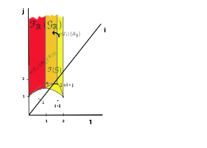
Figure I.1: Relation of Fundamental domains of $\Gamma$ and $\Gamma_{\mathbb{Z}}$

         Remark 3.2.11.

We also note for possible future reference that $\mathscr{F}_{\mathbb{R}}(\mathscr{G}_{\mathbb{R}})$ is the normal geodesic projection of the union of $\mathscr{F}(\mathscr{G})$ and one translate $\mathbf{c}(T_{1})\left(R_{\frac{\pi}{2}}^{2}\right)\mathscr{F}(\mathscr{G})$ of $\mathscr{F}(\mathscr{G})$. This relation between the fundamental domains is connected to the one given in Proposition 3.2.10, though neither relation implies the other, in general. In Figure 1, we have indicated by means of a “right-angle” symbol at the point $1+\sqrt{2}\mathbf{j}$ that the geodesic $\mathbb{H}^{1}(1+\sqrt{2}\mathbf{j},1+\mathbf{i}+\mathbf{j})$ is a geodesic normal to $\mathbb{H}^{2}_{\mathbf{j}}$. It would take us to far afield of our main purpose to define the concept of normal geodesic projection precisely, so for the moment we restrict ourselves to mentioning that this relation between $\mathscr{F}(\mathscr{G})$ and $\mathscr{F}_{\mathbb{R}}(\mathscr{G}_{\mathbb{R}})$ may be of some use in relating spectral expansions in the complex case to spectral expansions in the real case.

4 Volume Computations

4.1 Volumes

The following are reasons for computing the covolume of the lattices we are studying. First the volume computation is a relatively simple application of the previous results of a group-theoretic nature (that is, Lemmas 1.1.10 and (3.1.7)) to obtain quantitative geometric results that can be compared to previously obtained results in the literature. Second, the volume of the fundamental domain, or more precisely, the reciprocal of the volume of the fundamental domain under the Iwasawa-Haar measure, appears as a constant term in the Laplacian-eigenfunction expansion of automorphic functions. See, for example, [JL], Theorem XI.4.2, for the case of $\mathrm{SL}_{2}(\mathbb{Z}[\mathbf{i}])$ in $\mathrm{SL}_{2}(\mathbb{C})$. Therefore, the result of Corollary 4.3.13 will play a direct role in the next phase of this investigation. Third, covolume computations have applications in the theory of moduli space in algebraic geometry. For example, [GHS] uses a computation of the Hirzebruch-Mumford volume of an arithmetic lattice $\Gamma$ in a real form of $G$ to compute the leading term of growth of the space of cusp forms $S_{k}(\Gamma)$. The Hirzebruch-Mumford volume, which is defined precisely in [GHS], is a suitably normalized volume of the quotient $\Gamma\backslash G/K$. This, however, pertains to a future, projected stage of our project, in which the geometry of the fundamental domains and the eigenfunction expansion will be connected to the theory of certain moduli spaces of $K3$-surfaces.

4.2 Ratio of covolume of $\Gamma$, resp. $\Gamma_{\mathbb{Z}}$, to covolume of $\mathrm{SL}_{2}(\mathbb{Z}[\mathbf{i}])$, resp. $\mathrm{SL}_{2}(\mathbb{Z})$

         Lemma 4.2.1.

Let $X$ be a homogenous space of a semi-simple Lie group $G$, equipped with a $G$-invariant measure $\mu$. Let $\Gamma^{\prime}$, $\Gamma$ be commensurable lattices in $G$ which act on $X$ with finite volume quotient. Then we have

(4.2.1) $$\mu(M/\Gamma)=\mu(M/\Gamma^{\prime})\frac{[\Gamma^{\prime}:\Gamma^{\prime}\cap\Gamma]}{[\Gamma:\Gamma^{\prime}\cap\Gamma]}\vspace{0.3cm}$$

Proof. The lemma follows formally from the special case when $\Gamma^{\prime}\subseteq\Gamma$, i.e., when $[\Gamma^{\prime}:\Gamma^{\prime}\cap\Gamma]=1$. The reason is that we can apply the special case of (4.2.1) in the two cases

$$(\Gamma,\Gamma^{\prime})=(\Gamma,\Gamma^{\prime}\cap\Gamma)\;\text{resp.,}\;=(\Gamma^{\prime},\Gamma^{\prime}\cap\Gamma),\vspace{0.3cm}$$

then divide the results to deduce the general case of (4.2.1).

So assume that $\Gamma^{\prime}\subseteq\Gamma$, with $[\Gamma:\Gamma^{\prime}]=r\leq\infty$. By the assumption of commensurability there exists a finite set of elements $\gamma_{i}$, $i=1,\ldots,r$, with $r=[\Gamma:\Gamma^{\prime}]$, such that

$$\Gamma=\Gamma^{\prime}\gamma_{1}\cup\cdot\hskip 4.2679pt\cdots\cup\cdot\hskip 7.11317pt\Gamma^{\prime}\gamma_{r}.\vspace{0.3cm}$$

Let $\mathscr{F}$ be a fundamental domain for the action of $\Gamma$ on $X$. Set that

$$\mathscr{F}^{\prime}:=\gamma_{1}\mathscr{F}\cup\cdots\cup\gamma_{r}\mathscr{F},\;\text{with distinct translates disjoint, except for their common boundary.}\vspace{0.3cm}$$

then $\mathscr{F}^{\prime}$ is a fundamental domain for the action of $\Gamma^{\prime}$ on $X$, so that $\mu(\mathscr{F})=\mu(\Gamma\backslash M)$. The non-overlapping property of $\mathscr{F}$ for $\Gamma$ implies that the $\Gamma$-translates of $\mathscr{F}$ appearing in the union defining $\mathscr{F}^{\prime}$ intersect only on their boundaries, hence in sets of measure zero. Thus

$$\mu(\mathscr{F}^{\prime})=r\mu(\mathscr{F})=[\Gamma:\Gamma\cap\Gamma^{\prime}]\mu(\mathscr{F})\vspace{0.3cm}$$

Re-arranging, we obtain (4.2.1) in the special case, thus completing the proof. ∎

For the next proposition, let $\mu$ represent Iwasawa-Haar measure on $\mathrm{SL}_{2}(\mathbb{C})$, or $\mathrm{SL}_{2}(\mathbb{R})$, depending on the context. Using Lemma 1.1.10(b), resp., Lemma (3.1.7), we deduce from Lemma (4.2.1) formulas giving the covolumes of $\mathbf{c}^{-1}(\Gamma)$ and $\mathbf{c}^{-1}(\Gamma_{\mathbb{Z}})$, in terms of the covolumes of the standard integer subgroup, valid for any normalization of the Haar measure on $G$.

         Proposition 4.2.2.

Let $\Gamma=\mathrm{SO}_{3}(\mathbb{Z}[\mathbf{i}])$. Let $\mathbf{c}$ the isomorphism of $\mathrm{SL}_{2}(\mathbb{C})/\{\pm 1\}$ onto $\mathrm{SO}_{3}(\mathbb{C})$ induced by the conjugation action of $\mathrm{SL}_{2}(\mathbb{C})$ on its Lie algebra. Let $\Gamma_{\mathbb{Z}}\cong\mathrm{SO}(2,1)_{\mathbb{Z}}$ be as in Definition 3.1.1. Then we have

$$\mu(\mathbf{c}^{-1}(\Gamma)\backslash\mathrm{SL}_{2}(\mathbb{C}))=\frac{1}{2}\mu(\mathrm{SL}_{2}(\mathbb{Z}[\mathbf{i}])\backslash\mathrm{SL}_{2}(\mathbb{C})),\vspace{0.3cm}$$

and

$$\mu(\mathbf{c}^{-1}(\Gamma_{\mathbb{Z}})\backslash\mathrm{SL}_{2}(\mathbb{R}))=\frac{3}{2}\mu(\mathrm{SL}_{2}(\mathbb{Z})\backslash\mathrm{SL}_{2}(\mathbb{R})).\vspace{0.3cm}$$

Combining the well-known Corollary 4.3.13 (resp., 4.3.14), below, with Proposition 4.2.2, we determine the covolume of $\mathbf{c}^{-1}(\Gamma)$ (resp., $\mathbf{c}^{-1}(\Gamma_{\mathbb{Z}})$) in $\mathrm{SL}_{2}(\mathbb{C})$ (resp., $\mathrm{SL}_{2}(\mathbb{R})$).

         Corollary 4.2.3.

Let $\Gamma=\mathrm{SO}_{3}(\mathbb{Z}[\mathbf{i}])$. Let $\mathbf{c}$ the isomorphism of $\mathrm{SL}_{2}(\mathbb{C})/\{\pm 1\}$ onto $\mathrm{SO}_{3}(\mathbb{C})$ induced by the conjugation action of $\mathrm{SL}_{2}(\mathbb{C})$ on its Lie algebra. Let $\Gamma_{\mathbb{Z}}\cong\mathrm{SO}(2,1)_{\mathbb{Z}}$ be as in Definition 3.1.1. Then we have

$$\mu(\mathbf{c}^{-1}(\Gamma)\backslash\mathrm{SL}_{2}(\mathbb{C}))=\frac{1}{2}\mathbf{\Lambda}\zeta_{\mathbb{Q}(\mathbf{i})}(2).\vspace{0.3cm}$$

and

$$\mu(\mathbf{c}^{-1}(\Gamma_{\mathbb{Z}})\backslash\mathrm{SL}_{2}(\mathbb{R}))=\frac{3}{2}\mathbf{\Lambda}\zeta(2).\vspace{0.3cm}$$

4.3 Covolumes $V_{n}$ and $V_{n,\mathbb{R}}$ of Gaussian and rational integer subgroups.

Although the result of Corollary 4.3.13 is well-known, see e.g. [Lan66], the method, following Siegel’s proof of the rational-integer analogue, is not found in any standard reference. We include these results as an appendix in order to keep the treatment here of co-volumes self-contained and in order to show that there is a completely elementary route to the calculation of the covolumes in terms of special values of zeta functions.

Siegel’s Theorem on $V_{n}$.  In the following calculations, we closely follow the calculations in §${\mathrm{II}}$.4 of [JL05]. There, one finds an elementary calculation, following the approach of Siegel, resulting in 4.1.3, the covolume of $\mathrm{SL}_{n}(\mathbb{Z})$ in $\mathrm{SL}_{n}(\mathbb{R})$. In the following arguments, culminating in Theorem 4.3.4, and Corollary 4.3.13 we in effect show that the arguments of [JL05], §${\mathrm{II}}$.4, transfer in the most direct imaginable manner to the Gaussian integer case. Although, for the case at hand, we only need the case $n=2$, it is natural to treat the case of general $n$. The treatment of the quadratic models $\mathrm{Pos_{n}}(\mathbb{C})$ and $\mathrm{Spos}_{n}(\mathbb{C})$ and the decomposition of the $G$-invariant measures on these spaces will be useful for the extension of the theory of the present monograph to higher rank.

         Definition 4.3.1.

The Dedekind Zeta function $\zeta_{\mathbb{Q}(\mathbf{i})}$ associated to the number field $\mathbb{Q}(\mathbf{i})$  is defined by

(4.3.1) $$\zeta_{\mathbb{Q}(\mathbf{i})}(s) = \sum_{I\;\text{ideal of}\;\mathbb{Z}[\mathbf{i}]}N(I)^{-s}$$

$$= \sum_{\ell\;\text{standard}}||\ell||^{-2s},$$

where, in the first line, $N$ denotes the norm from $\mathbb{Q}(\mathbf{i})$ to $\mathbb{Q}$, and in the second line, the sum is over all standard elements of the ring $\mathbb{Z}[\mathbf{i}]$, in the sense defined in §1.1.

The expression for $\zeta_{\mathbb{Q}(\mathbf{i})}$ given in the first line of (4.3.1) is stated in terms of notions which generalize to an arbitrary number fields $F$, and thus gives the definition of the Dedekind zeta function associated to $F$. In order to pass from the expression in the first line of (4.3.1) to that of the second line, one uses the well-known characterization of the norm,

$$N(I)=\#(\mathfrak{o}/I).\vspace{0.3cm}$$

Then one applies the one-to-one correspondence between ideals of the principal ring $\mathbb{Z}[\mathbf{i}]$ and standard integers (assigning to the ideal $I$ its unique standard generator $\ell$), and one easily calculates

$$N(I)=\#(\mathbb{Z}[\mathbf{i}]/I)=\#(\mathbb{Z}[\mathbf{i}]/(\ell))=||\ell||^{2}.\vspace{0.3cm}$$

We tabulate some subgroups of $\mathrm{SL}_{n}(\mathbb{C})$ which will allow inductive decompositions.

(4.3.2) $$G_{n} = \mathrm{SL}_{n}(\mathbb{C}).$$

$$\Gamma_{n} = \mathrm{SL}_{n}(\mathbb{Z}[\mathbf{i}]).$$

$$G_{n,n} = G_{n} n^{\rm th}$$ subgroup of leaving the unit vector fixed.

$$\Gamma_{n,n} = \Gamma_{n}\cap G_{n,n}.$$

Scholium on $G_{n,n}$.  Subgroups of $G$ defined by a condition of the type used in (4.3.2) to define $G_{n,n}$ are known in the literature as mirabolic subgroups. Specifically, $G_{n,n}$ is known as the mirabolic subgroup associated to the maximal parabolic preserving the the flag $\{\mathbb{C}e_{n}\}$. Directly from the definition of $G_{n,n}$ in (4.3.2), we compute that

(4.3.3) $$G_{n,n}=\left\{\left.\begin{pmatrix}g^{\prime}&\mathbf{x}\\ 0&1\end{pmatrix}\;\right|\;\mathbf{x}^{*}\in\mathbb{C}^{n-1},\;g^{\prime}\in\mathrm{SL}_{n-1}(\mathbb{C})\right\}.\vspace{0.3cm}$$

To facilitate comparison with [JL05], we note here that we diverge from their notation in keeping the subscript $n$, on $G_{n}$, and its associated objects ($G_{n,n}$, $\Gamma_{n,n}$ ,etc.) This subscript is maintained in order to distinguish the discrete groups being considered here (the $\mathrm{SL}_{n}(\mathbb{Z}[\mathbf{i}])$) from the discrete group $\Gamma=\mathrm{SO}_{3}(\mathbb{Z}[\mathbf{i}])$ under consideration in the other sections of this chapter.

There is a natural isomorphism of $G_{n}$-homogeneous spaces

(4.3.4) $$G_{n,n}\backslash G_{n}\stackrel{{\scriptstyle\approx}}{{\longrightarrow}}(\mathbb{C}^{n})^{*}-\{0\}\;\;\text{given by}\;g\mapsto e_{n}^{*}g.\vspace{0.3cm}$$

We have a fibering

(4.3.5) $$\mathbb{Z}[\mathbf{i}]^{n-1}\backslash\mathbb{C}^{n-1}\rightarrow\Gamma_{n,n}\backslash G_{n,n}\rightarrow\Gamma_{n-1}\backslash G_{n-1}=\mathrm{SL}_{n-1}(\mathbb{Z}[\mathbf{i}])\backslash\mathrm{SL}_{n-1}(\mathbb{C}).\vspace{0.3cm}$$

arising from the coordinates $(\mathbf{x},g^{\prime})$ on $G_{n,n}$, above, in (4.3.3). From the fibration in (4.3.5), we deduce that $\Gamma_{n,n}\backslash G_{n,n}$ has finite measure, under the inductive assumption that $\Gamma_{n-1}\backslash G_{n-1}$ has finite measure.

Because of (4.3.4), we can transport Lebesgue measure from $\mathbb{C}^{n}\approx\mathbb{R}^{2n}$ to $G_{n,n}\backslash G_{n}$. We use $\mathbf{x}$ for the variable on $\mathbb{R}^{2n}$, sometimes identified with the variable in $G_{n,n}\backslash G_{n}$. In an integral, we write Lebesgue measure as $\,\mathrm{d}\mathbf{x}$. We let $\mu_{G_{n,n}\backslash G_{n}}$ be the corresponding measure on $G_{n,n}\backslash G_{n}$, under the isomorphism (4.3.4).

Recall throughout the following discussion that a homogeneous space of a closed unimodular linear group has an invariant measure, unique up to constant factor. Consider the lattice of subgroups

(4.3.6) $$\begin{diagram}\vspace{0.3cm}$$

Fix a Haar measure $\,\mathrm{d}g_{n}$ on $G$. On the discrete groups $\Gamma_{n}$, $\Gamma_{n,n}$, let Haar measure be the counting measure. Then $\,\mathrm{d}g_{n}$ determines unique measures on $\Gamma_{n}\backslash G_{n}$ and $\Gamma_{n,n}\backslash G_{n}$, since the measure is determined locally. We write $\,\mathrm{d}\overline{g}_{n}$ for each of these induced measures from the right hand side of the diagram in (4.3.7). Passing to the left-hand side of (4.3.7), having fixed $\,\mathrm{d}g_{n}$ on $G_{n}$ and

$$\,\mathrm{d}\mu_{G_{n,n}\backslash G_{n}}=\,\mathrm{d}\mathbf{x}\;\text{on}\;G_{n,n}\backslash G_{n},\vspace{0.3cm}$$

there is a unique measure $\,\mathrm{d}G_{n,n}$ on $G_{n,n}$ such that

(4.3.7) $$\int_{G_{n,n}\backslash G_{n}}\int_{\Gamma_{n,n}\backslash G_{n,n}}=\int_{\Gamma_{n,n}\backslash G_{n}}=\int_{\Gamma_{n}\backslash G_{n}}\int_{\Gamma_{n,n}\backslash\Gamma_{n}}.\vspace{0.3cm}$$

The integration formula (4.3.7) is meant to be interpreted as two Fubini-type theorems for the evaluation of an integral on the space $L^{1}(\Gamma_{n,n}\backslash G_{n})$.

         Lemma 4.3.2.

Let $f\in L^{1}(\mathbb{R}^{2n})\approx L^{1}(G_{n,n}\backslash G_{n})$. Let $c_{n}=\mathrm{vol}(\Gamma_{n,n}\backslash G_{n,n})$, as measured by $\,\mathrm{d}\overline{g}_{n,n}$. Then

$$c_{n}\int_{\mathbb{R}^{n}}f(\mathbf{x})\,\mathrm{d}\mathbf{x}=\int_{\Gamma_{n}\backslash G_{n}}\int_{\Gamma_{n,n}\backslash\Gamma_{n}}f(\gamma g)\,\mathrm{d}\overline{\gamma_{n}}\,\mathrm{d}\overline{g}_{n}.\vspace{0.3cm}$$

Proof. Since $L^{1}(G_{n,n}\backslash G_{n})$ is a subspace $L^{1}(\Gamma_{n,n}\backslash G_{n})$, we can apply the Fubini-type integral formula (4.3.7) to $f$. Because of the invariance property of $f$, the inner integral on the left-side of (4.3.7) reduces to $c_{n}$. ∎

Denote by $\textbf{prim}(\mathbb{Z}[\mathbf{i}]^{n})^{*}$  the set of primitive $n$-vectors, i.e., integral vectors such that the GCD of the components is $1$. See Definition 1.1.3 and the following properties following it for a review of the GCD in the context of pairs Gaussian integers. The definition and properties have obvious extensions to $n$-tuples of Gaussian integers, which we will use freely in what follows. We will also make free use of the “Conventions regarding multiplicative structure of $\mathbb{Z}[\mathbf{i}]$” in the paragraph preceding that definition.

Since $\text{prim}(\mathbb{Z}[\mathbf{i}]^{n})^{*}$ is precisely the set of vectors in $(\mathbb{Z}[\mathbf{i}]^{n})^{*}$ which can be extended to a matrix in $\Gamma_{n}=\mathrm{SL}_{n}(\mathbb{Z}[\mathbf{i}])$, we have

(4.3.8) $$e_{n}^{*}\Gamma_{n}=e_{n}^{*}\mathrm{SL}_{n}(\mathbb{Z}[\mathbf{i}])=\text{prim}(\mathbb{Z}[\mathbf{i}]^{n})^{*}.\vspace{0.3cm}$$

Next, we claim that we have

(4.3.9) $$(\mathbb{Z}[\mathbf{i}]^{n})^{*}-\{0\}=\{\ell\mathbf{v}\;\text{with}\;\mathbf{v}\;\text{primitive and}\;\ell\in\mathbb{Z}[\mathbf{i}]-\{0\}\;\text{standard}\},\vspace{0.3cm}$$

where the decomposition of $\mathbf{w}\in(\mathbb{Z}[\mathbf{i}]^{n})^{*}$ into $\ell$ and $\mathbf{v}$ is understood be unique. In order prove the claim, for an arbitrary element $\mathbf{w}\in(\mathbb{Z}[\mathbf{i}]^{n})^{*}-\{0\}$, set $\ell$ equal to the GCD of the entries of $\mathbf{w}$. Then set

$$\mathbf{v}=\ell^{-1}\mathbf{w}.\vspace{0.3cm}$$

Use Properties GCD 1 and GCD 2 (more precisely, the form of the properties extended to $n$-tuples) to see that $\mathbf{v}$ is primitive. If $\ell^{\prime}\mathbf{v}^{\prime}$ is another decomposition of $\mathbf{w}$ in the form given in (4.3.9), then

$${\ell^{\prime}}^{-1}\ell\mathbf{v}=\mathbf{v}^{\prime},\vspace{0.3cm}$$

with both $\mathbf{v},\,\mathbf{v}^{\prime}$ primitive. So ${\ell^{\prime}}^{-1}\ell$ is a unit. Since $\ell,\ell^{\prime}$ are standard, the unit in question must be $1$. Thus $\ell=\ell^{\prime}$, and we deduce the uniqueness of the decomposition.

         Remark 4.3.3.

The decomposition (4.3.9) corresponds to the displayed equation immediately following (5) in §${\mathrm{II}}$.4 in [JL05], with the condition that “$k$” (the $\ell$ of our notation) is positive corresponding to the condition that our $\ell$ is standard. In fact, the condition of standard-ness is an appropriate generalization of positivity from the context of the multiplicative theory of $\mathbb{Z}$ to the multiplicative theory of $\mathbb{Z}[\mathbf{i}]$.

Let

$$V_{n}=\mathrm{vol}(\Gamma_{n}\backslash G_{n})=\mathrm{vol}(\mathrm{SL}_{n}(\mathbb{Z}[\mathbf{i}])\backslash\mathrm{SL}_{n}(\mathbb{C})).\vspace{0.3cm}$$

If we change the Haar measure on $G$ by a constant factor, then the volume changes by this same constant. The volume is with respect to our fixed $\,\mathrm{d}g_{n}$. In (4.3.26), below, we shall fix a normalization of $\,\mathrm{d}g_{n}$.

In the proof of Theorem 4.3.4 below, we will use the following change of variables formula.

(4.3.10) $$\int_{\mathbb{C}^{n}}f(y\mathbf{x})\,\mathrm{d}\mathbf{x}=||y||^{-2n}\int_{\mathbb{C}^{n}}f(\mathbf{x})\,\mathrm{d}\mathbf{x},\;\text{for}\;f\in\L^{1}(\mathbb{C}^{n}),\;y\in\mathbb{C}^{\times}.\vspace{0.3cm}$$

The formula (4.3.10) is derived by computing the Jacobian factor of the multiplication endomorphism of $\mathbb{C}^{n}$ given by $\mathbf{x}\mapsto y\mathbf{x}$. Clearly, the Jacobian of the multiplication endomorphism is independent of $\arg(y)$, so is a function of $||y||$ alone. The Jacobian factor is clearly mutliplicative in $y$, hence a power of $||y||$. Then exponent of $||y||$ in the Jacobian is determined by noting that the dimension of $\mathbb{C}^{n}$ as a real vector space is $2n$.

         Theorem 4.3.4.

After Siegel [Sie45]. Let $G_{n}=\mathrm{SL}_{n}(\mathbb{C})$, $\Gamma_{n}=\mathrm{SL}_{n}(\mathbb{Z}[\mathbf{i}])$. Let $\,\mathrm{d}\mathbf{x}$ be the Lebesgue measure on $\mathbb{C}^{n}\approx\mathbb{R}^{2n}$. Let $\mathbf{w}$ denote a length-$n$ vector with entries in $\mathbb{Z}[\mathbf{i}]$. Let $f\in L^{1}(\mathbb{C}^{n})\cong L^{1}(\mathbb{R}^{2n})$. Then

$$V_{n}\int_{\mathbb{R}^{2n}}f(\mathbf{x})\,\mathrm{d}\mathbf{x} = \int_{\Gamma_{n}\backslash G_{n}}\sum_{\mathbf{w}\neq 0}f(\mathbf{w}g)\,\mathrm{d}\overline{g}$$

$$= \zeta_{\mathbb{Q}(\mathbf{i})}(n)\int_{\Gamma\backslash G}\sum_{\mathbf{v}\;\text{prim}}f(\mathbf{v}g)\,\mathrm{d}\overline{g}.$$

Furthermore, $V_{n}=c_{n}\zeta_{\mathbb{Q}(\mathbf{i})}(n)$. Corollary 4.3.13, below, will determine $V_{n},c_{n}$.

Proof. On the right side of (4.3.7), we use Lemma 4.3.2 to obtain

$$\int_{\Gamma_{n}\backslash G_{n}}\sum_{\mathbf{v}\;\text{prim}}f(\mathbf{v}g)d\overline{g}=c_{n}\int_{\mathbb{C}^{n}}f(\mathbf{x})\,\mathrm{d}\mathbf{x}.\vspace{0.3cm}$$

Replacing $f(x)$ by $f(\ell\mathbf{x})$ with $\ell$ a standard integer $\ell$, and using (4.3.10) on the right, we find

(4.3.11) $$\int_{\Gamma_{n}\backslash G_{n}}\sum_{\mathbf{v}\;\text{prim}}f(\ell\mathbf{v}g)\,\mathrm{d}\overline{g}=c_{n}||\ell||^{-2n}\int_{\mathbb{C}^{n}}f(\mathbf{x})\,\mathrm{d}\mathbf{x}.\vspace{0.3cm}$$

Summing over all standard $\ell\in\mathbb{Z}[\mathbf{i}]$, the elements $\ell\mathbf{v}$ range over all nonzero elements $\mathbf{w}\in(\mathbb{Z}[\mathbf{i}]^{n})^{*}$, taking each value once, by (4.3.9). Thus, the summed form of the left-hand side of (4.3.11) gives the left-hand side of (4.3.12), below. In order to see that the summed form of the right-hand side of (4.3.11) gives the right-hand side of (4.3.12), we use the expression for $\zeta_{\mathbb{Q}(\mathbf{i})}$ given in the second line of (4.3.1). Thus, we obtain

(4.3.12) $$\int_{\Gamma_{n}\backslash G_{n}}\sum_{\mathbf{w}\neq 0}f(\mathbf{w}g)\,\mathrm{d}\overline{g}=c_{n}\zeta_{\mathbb{Q}(\mathbf{i})}(n)\int_{\mathbb{C}^{n}}f(\mathbf{x})\,\mathrm{d}\mathbf{x}.\vspace{0.3cm}$$

Assuming that $V_{n}$ is finite, we shall now prove that $V_{n}=c_{n}\zeta_{\mathbb{Q}(\mathbf{i})}(n)$. For this, we can take a function $f$ which is continuous, $\geq 0$, with positive integral and compact support. We note that for any $g\in\mathrm{SL}_{n}(\mathbb{C})$,

(4.3.13) $$\lim_{N\rightarrow\infty}\frac{1}{N^{2n}}\sum_{\mathbf{w}\neq 0}f\left(\frac{1}{N}\mathbf{w}g\right)=\int_{\mathbb{C}^{n}}f(\mathbf{x})\,\mathrm{d}\mathbf{x},\vspace{0.3cm}$$

The reason is that the left-hand side of (4.3.13), without the limit, is the Riemann sum for the integral on the right-hand side associated to a subdivision of the support of $f$ into parallelotopes of side-length $\frac{1}{N}$. The right-multiplication by $g\in\mathrm{SL}_{n}(\mathbb{C})$ changes the side lengths of a parallelotope, but preserves the volume. Integrating (4.3.13) over $\Gamma_{n}\backslash G_{n}$, we find

$$V_{n}\int_{\mathbb{C}^{n}}f(\mathbf{x})\,\mathrm{d}\mathbf{x} = \int_{\Gamma_{n}\backslash G_{n}}\lim_{N\rightarrow\infty}\frac{1}{N^{2n}}\sum_{\mathbf{w}\neq 0}f\left(\frac{1}{N}\mathbf{w}g\right)\,\mathrm{d}\overline{g}$$

$$= \lim_{N\rightarrow\infty}\frac{1}{N^{2n}}\int_{\Gamma_{n}\backslash G_{n}}\sum_{\mathbf{w}\neq 0}f\left(\frac{1}{N}\mathbf{w}g\right)\,\mathrm{d}\overline{g}$$

$$= \lim_{N\rightarrow\infty}c_{n}\zeta_{\mathbb{Q}(\mathbf{i})}(n)\frac{1}{N^{2n}}\int_{\mathbb{C}^{n}}f\left(\frac{1}{N}\mathbf{x}\right)\,\mathrm{d}\mathbf{x} (\text{by}\;\eqref{eqn:siegelsthminter2})$$

$$= \lim_{N\rightarrow\infty}c_{n}\zeta_{\mathbb{Q}(\mathbf{i})}(n)\int_{\mathbb{C}^{n}}f(\mathbf{x})\,\mathrm{d}\mathbf{x} (\text{by letting}\;u=\mathbf{x}/N,\;\,\mathrm{d}u=\,\mathrm{d}\mathbf{x}/N^{2n}).$$

This concludes the proof of Siegel’s theorem. ∎

Decompositions of invariant measure on $\mathrm{Pos}_{n}(\mathbb{C})$

         Definition 4.3.5.

The space $\mathrm{Pos}_{n}(\mathbb{C})$  is defined to be the Hermitian matrices of size $n$, having positive eigenvalues. The group $\mathrm{GL}_{n}(\mathbb{C})$ acts on $\mathrm{Pos}_{n}(\mathbb{C})$ on the left, according to the formula

(4.3.14) $$[g]p\mapsto gpg^{*},\vspace{0.3cm}$$

and $\mathrm{Pos}_{n}(\mathbb{C})$ is a $\mathrm{GL}_{n}(\mathbb{C})$-homogeneous space. Accordingly, it has a $\mathrm{GL}_{n}(\mathbb{C})$-invariant measure, which is unique up to a constant factor.

For the purposes of comparison, we introduce the following notation for the Lebesgue measure on a Euclidean space with a system of coordinates $Y=\left((y_{ij}^{\left(\mathbf{i}^{\delta}\right)}\right)$ where the coordinate $y_{ij}^{(1)}$ corresponds to the real component and $y_{ij}^{({\mathbf{i}})}$ to the imaginary component of $y_{ij}$. We write

$$\,\mathrm{d}\mu_{\mathrm{euc}}(Y)=\prod\,\mathrm{d}y_{ij}^{\left(\mathbf{i}^{\delta}\right)},\;\text{where}\;1\leq i\leq j\leq n,\;\text{and}\;\delta=\begin{cases}0,1&\text{for}\;i<j\\ 0&\text{for}\;i=j\end{cases}\,.\vspace{0.3cm}$$

Here are some comments on the notation to be used below. We shall reserve the letter $Y$ for a variable in $\mathrm{Pos}_{n}(\mathbb{C})$, and $Z$ for a variable in the space $\mathrm{Spos}_{n}(\mathbb{C})$, introduced in Definition 4.3.8 below. Deviations from Lebesgue measure will be denoted by $\,\mathrm{d}\mu(Y)$, with $\mu$ to be specified. If $\varphi$ is a local $C^{\infty}$ isomorphism, $J(\varphi)$ will denote the Jacobian factor of the induced map on the measure, so the absolute value of the determinant of the Jacobian matrix, when expressed in terms of local coordinates. If $g$ is a square matrix, we let $|g|$ denote its determinant and $||g||$ the absolute value of the determinant.

         Proposition 4.3.6.

A $\mathrm{GL}_{n}(\mathbb{C})$-bi-invariant measure on $\mathrm{Pos}_{n}(\mathbb{C})$ is given by

(4.3.15) $$\,\mathrm{d}\mu_{n}(Y)=|Y|^{-n}\,\mathrm{d}\mu_{\mathrm{euc}}(Y).\vspace{0.3cm}$$

For $g\in\mathrm{GL}_{n}(\mathbb{C})$, the Jacobian determinant $J(g)$ of the determinant of the transformation $[g]$ is

$$J(g)=||g||^{2n}.\vspace{0.3cm}$$

The invariant measure satisfies $\,\mathrm{d}\mu_{n}(Y^{{}^{-1}})=\,\mathrm{d}\mu_{n}(Y)$, i.e. it is also invariant under $Y\mapsto Y^{-1}$.

Proof. We prove the second assertion first. Note that $g\mapsto J(g)$ is multiplicative and continuous, so that it suffices to prove the formula for a dense set of matrices $g$. We pick the set of semisimple matrices in $\mathrm{GL}_{n}(\mathbb{C})$, i.e., those of the form

$$gDg^{-1},\;\text{with}\;D=\mathrm{diag}(d_{1},\ldots,d_{n}),\;g\in\mathrm{GL}_{n}(\mathbb{C}).\vspace{0.3cm}$$

Then we readily calculate that

$$[D]Y=(d_{i}y_{ij}\overline{d_{j}}),\vspace{0.3cm}$$

so that, by the multiplicativity of $J$,

$$J(gDg^{-1})=J(D)=\prod_{1\leq i<j\leq n}|d_{i}d_{j}|^{2}\prod_{1\leq i\leq n}|d_{i}|^{2}=||D||^{2(n-1)}||D||^{2}=||D||^{2n}=||gDg^{-1}||^{2n},\vspace{0.3cm}$$

which, by the above comments, proves the formula for $J(g)$. Then, with $\,\mathrm{d}\mu_{n}$ defined as in (4.3.15),

$$\,\mathrm{d}\mu_{n}([g]Y) = |[g]Y|^{-n}J([g])\,\mathrm{d}\mu_{\rm euc}(Y)$$

$$= ||g||^{-2n}|Y|^{-n}||g||^{2n}\,\mathrm{d}\mu_{\rm euc}(Y)$$

$$= \,\mathrm{d}\mu_{n}(Y),$$

thus concluding the proof of left invariance. Right invariance follows because $J(g)=J(g^{*})$.

Finally, the invariance under $Y\mapsto Y^{-1}$ follows because if we let $S(Y)=Y^{-1}$, then for a tangent vector $H\in\mathrm{Herm}_{n}$,

$$S^{\prime}(Y)H=-Y^{-1}HY^{-1},\vspace{0.3cm}$$

so $\det S^{\prime}(Y)=J(Y^{-1})=|Y|^{-2n}$. Then

$$\,\mathrm{d}\mu_{n}(Y^{-1})=|Y|^{n}|Y|^{-2n}\,\mathrm{d}\mu_{\rm euc}(Y)=|Y|^{-n}\,\mathrm{d}\mu_{\rm euc}(Y)=\,\mathrm{d}\mu_{n}(Y),\vspace{0.3cm}$$

thus concluding the proof of the proposition. ∎

We have the first order partial Iwasawa decomposition of $Y\in\mathrm{Pos}_{n}(\mathbb{C})$:

(4.3.16) $$Y=\begin{bmatrix}I_{n-1}&\mathbf{x}\\ 0&1\end{bmatrix}\begin{pmatrix}W&0\\ 0&v\end{pmatrix},\vspace{0.3cm}$$

with $v\in\mathbb{R}^{+},\,\mathbf{x}^{*}\in\mathbb{C}^{n-1},\,W\in\mathrm{Pos}_{n-1}(\mathbb{C})$

The decomposition (4.3.16) gives first partial coordinates $Y=Y(W,\mathbf{x},v)$, with the map

$$\varphi^{+}_{n-1,1}:\mathrm{Spos_{n-1}(\mathbb{C})}\times{\mathbb{C}^{n-1}}^{*}\times\mathbb{R}^{+}\rightarrow\mathrm{Spos}_{n}(\mathbb{C}),\vspace{0.3cm}$$

as in (4.3.16) as above. Direct multiplication in (4.3.16) yields the explicit explicit expression

(4.3.17) $$\varphi^{+}_{n-1,1}(W,\mathbf{x},v)=\begin{pmatrix}v^{-\frac{1}{n-1}}W+v\mathbf{x}^{*}\mathbf{x}&v\mathbf{x}\\ v\mathbf{x}^{*}&v\end{pmatrix}.\vspace{0.3cm}$$

From (4.3.17), we see that $\varphi^{+}_{n-1,1}$ is bijective, because, first $v\in\mathbb{R}^{+}$ uniquely determines the lower right entry. Then $\mathbf{x}\in{\mathbb{C}^{n-1}}^{*}$ is uniquely determined to give the last row (or last column), and finally $W$ is uniquely determined by the upper-left $(n-1)\times(n-1)$ square.

We wish to compare the partial Iwasawa coordinates in (4.3.17) with the coordinates on $\mathrm{Pos}_{n}(\mathbb{C})$ induced by the block decomposition

$$Y=\begin{pmatrix}Y_{1}&\mathbf{y_{2}}\\ \mathbf{y_{2}}^{*}&y_{3}\end{pmatrix}\vspace{0.3cm}$$

where $Y_{1}$ is an $(n-1)\times(n-1)$ matrix, $\mathbf{y_{2}}$ is an $(n-1)$-vector, and $y_{3}>0$.

         Proposition 4.3.7.

The Jacobian is given by

$$J(\varphi^{+}_{n-1,1})=|V|^{2(n-1)}.\vspace{0.3cm}$$

For $Y=\varphi^{+}(W,\mathbf{x},v)$ we have the change of variable formula

$$\,\mathrm{d}\mu_{n}(Y)=|W|^{-1}v^{n-1}\,\mathrm{d}\mu_{\rm euc}(X)\,\mathrm{d}\mu_{n-1}(W)\,\mathrm{d}\mu_{1}(v)\vspace{0.3cm}$$

Proof. We compute the Jacobian matrix and find

$$\frac{\partial(Y)}{\partial(W,\mathbf{x},v)}=\begin{pmatrix}I_{(n-1)^{2}}&*\cdots*&*\\ 0&v\cdots 0&*\\ \vdots&\vdots\ddots\vdots&\vdots\\ 0&0\cdots v&*\\ 0&0\cdots 0&1\end{pmatrix},\vspace{0.3cm}$$

with $v$ occuring $2(n-1)$ times on the diagonal. Taking the determinant yields the stated value. For the change of variable formula, we just plug in using the definitions

$$\,\mathrm{d}\mu_{n-1}(W)=|W|^{-(n-1)}\,\mathrm{d}\mu_{\rm euc},\vspace{0.3cm}$$

and similarly with $n$ and $1$, combined with the value for the Jacobian. The formula comes out as stated. ∎

Decompositions of invariant measure on $\mathrm{SPos}_{n}(\mathbb{C})$

         Definition 4.3.8.

We define $\mathbf{Spos}_{n}(\mathbb{C})$  to be the subspace of $\mathrm{Pos}_{n}(\mathbb{C})$ consisting of unimodular matrices. The unimodular subgroup $\mathrm{SL}_{n}(\mathbb{C})$ acts on $\mathrm{Spos}_{n}(\mathbb{C})$ by the same formula (4.3.14), and $\mathrm{Spos}_{n}(\mathbb{C})$ is an $\mathrm{SL}_{n}(\mathbb{C})$-homogeneous space. It therefore has a $\mathrm{SL}_{n}(\mathbb{C})$-invariant measure, unique up to constant factor. Every $Y\in\mathrm{Pos}_{n}(\mathbb{C})$ can be written uniquely in the form

$$Y=r^{1/n}Z\;\text{with}\;r>0\;\text{and}\;Z\in\mathrm{Spos}_{n}(\mathbb{C}).\vspace{0.3cm}$$

Thus, we have a product decomposition

(4.3.18) $$\mathrm{Pos}_{n}(\mathbb{C})=\mathbb{R}^{+}\times\mathrm{Spos}_{n},\vspace{0.3cm}$$

in terms of the coordinates $(r,Z)$. We denote by $\mu_{n}^{(1)}$ the $\mathrm{SL}_{n}(\mathbb{C})$-invariant measure on $\mathrm{Spos}_{n}(\mathbb{C})$ such that for the product decomposition (4.3.18) we have

(4.3.19) $$\,\mathrm{d}\mu_{n}(Y)=\frac{\,\mathrm{d}r}{r}\,\mathrm{d}\mu_{n}^{(1)}(Z).\vspace{0.3cm}$$

We have the first order partial Iwasawa decomposition of $Z\in\mathrm{Spos}_{n}(\mathbb{C})$:

(4.3.20) $$Z=\begin{bmatrix}I_{n-1}&\mathbf{x}\\ 0&1\end{bmatrix}\begin{pmatrix}v^{-1/(n-1)}W&0\\ 0&v\end{pmatrix},\;\text{with $v\in\mathbb{R}^{+},\,\mathbf{x}^{*}\in\mathbb{C}^{n-1},\,W\in\mathrm{SPos}_{n-1}(\mathbb{C})$.}\vspace{0.3cm}$$

Note that, by multiplying out the right-hand side of (4.3.20) and comparing lower-right entries, we obtain

(4.3.21) $$z_{nn}=v\vspace{0.3cm}$$

The decomposition (4.3.20) gives first partial coordinates $Y=Y(W,\mathbf{x},v)$, with the map

$$\varphi^{+}_{n-1,1}:\mathbb{R}^{+}\times{\mathbb{C}^{n-1}}^{*}\times\mathrm{Spos_{n-1}(\mathbb{C})}\rightarrow\mathrm{Spos}_{n}(\mathbb{C}),\vspace{0.3cm}$$

as in (4.3.20) as above. Direct multiplication in (4.3.20) yields the explicit expression

(4.3.22) $$\varphi^{+}_{n-1,1}(W,\mathbf{x},v)=\begin{pmatrix}v^{-1/n-1}W+v\mathbf{x}^{*}\mathbf{x}&v\mathbf{x}\\ v\mathbf{x}^{*}&v\end{pmatrix}.\vspace{0.3cm}$$

From (4.3.22), we see that $\varphi^{+}_{n-1,1}$ is bijective, because, first $v\in\mathbb{R}^{+}$ uniquely determines the lower right entry. Then $\mathbf{x}\in{\mathbb{C}^{n-1}}^{*}$ is uniquely determined to give the last row (or last column), and finally $W$ is uniquely determined by the upper-left $(n-1)\times(n-1)$ square.

         Proposition 4.3.9.

Associated to the first partial Iwasawa decomposition of (4.3.20), we have the measure decomposition

$$\,\mathrm{d}\mu_{n}^{(1)}(Z)=v^{n}\frac{\,\mathrm{d}v}{v}\,\mathrm{d}\mathbf{x}\,\mathrm{d}\mu_{n-1}^{(1)}(W).\vspace{0.3cm}$$

Proof. Write the first-partial Iwasawa decomposition of $Y\in\mathrm{Pos}_{n}(\mathbb{C})$ in the form

$$Y=\begin{bmatrix}I_{n-1}&\mathbf{x}\\ &1\end{bmatrix}\begin{pmatrix}{v^{\prime}}^{-1/n-1}W&\\ &v\end{pmatrix}\vspace{0.3cm}$$

with $W\in\mathrm{Spos}_{n}(\mathbb{C})$. Let $r=|Y|$, so that

$$Y=r^{1/n}Z,\;\text{with}\;Z\in\mathrm{Spos}_{n}(\mathbb{C}).\vspace{0.3cm}$$

On the one hand, by (4.3.19), we have

(4.3.23) $$\,\mathrm{d}\mu_{n}(Y)=\frac{\,\mathrm{d}r}{r}\,\mathrm{d}\mu_{n}^{(1)}(Z).\vspace{0.3cm}$$

On the other hand, we have, by (4.3.15),

(4.3.24) $$\,\mathrm{d}\mu_{n}(Y) = |Y|^{-n}\,\mathrm{d}\mu_{\rm euc}(Y)$$

$$= |Y|^{-n}v^{2(n-1)}\,\mathrm{d}\mu_{\rm euc}(\mathbf{x})\,\mathrm{d}\mu_{\rm euc}(v)\,\mathrm{d}\mu_{\rm euc}({v^{\prime}}^{-1/n-1}W) (\text{by Proposition}\;\ref{prop:partialawasawajacobian})$$

$$= |Y|^{-n}v^{2n-1}\frac{\,\mathrm{d}v}{v}\,\mathrm{d}\mathbf{x}\,\mathrm{d}\mu_{\rm euc}({v^{\prime}}^{-1/n-1}W)$$

$$= |Y|^{-n}v^{2n-1}|v^{-1/n-1}W|^{n-1}\,\mathrm{d}\mu_{n-1}({v^{\prime}}^{-1/n-1}W)\frac{\,\mathrm{d}v}{v}\,\mathrm{d}\mathbf{x} (\text{by \eqref{eqn:posncmeasuredefn}}).$$

Now set $r^{\prime}=\frac{1}{v^{\prime}}$, so that

$${v^{\prime}}^{1/n-1}W={r^{\prime}}^{1/n-1}W\;\text{with}\;W\in\mathrm{Spos}_{n}(\mathbb{C}),\vspace{0.3cm}$$

and

$$\,\mathrm{d}\mu_{n-1}({v^{\prime}}^{-1/n-1}W)=\frac{\,\mathrm{d}r^{\prime}}{r^{\prime}}\,\mathrm{d}\mu_{n-1}^{(1)}(W).\vspace{0.3cm}$$

Thus, from (4.3.24), we have

(4.3.25) $$\,\mathrm{d}\mu_{n}(Y) = v^{\prime}v^{n-1}\left(\frac{\,\mathrm{d}r^{\prime}}{r^{\prime}}\,\mathrm{d}\mu_{n-1}^{(1)}(W)\right)\frac{\,\mathrm{d}v}{v}\,\mathrm{d}\mathbf{x}$$

$$= \left(\frac{\,\mathrm{d}r^{\prime}}{r^{\prime}}\right)v^{\prime}v^{n-1}\,\mathrm{d}\mu_{n-1}^{(1)}(W)\frac{\,\mathrm{d}v}{v}\,\mathrm{d}\mathbf{x}$$

$$= \left(\frac{\,\mathrm{d}r}{r}\right)v^{n}\,\mathrm{d}\mu_{n-1}^{(1)}(W)\frac{\,\mathrm{d}v}{v}\,\mathrm{d}\mathbf{x},$$

where the last line follows because $r^{\prime}=r$ and $v^{\prime}=v$ for $Y\in\mathrm{Spos}_{n}(\mathbb{C})$. ∎

The measure decomposition of Proposition 4.3.9 gives rise to a corresponding measure decomposition on the fibration. In terms of integration over the fibers, we get the following integral formula.

         Proposition 4.3.10.

For a function $f$ on $\Gamma_{n,n}\backslash\mathrm{Spos}_{n}$, in terms of the coordinates of Proposition 4.3.9, we have

$$\int_{\Gamma_{n,n}\backslash\mathrm{Spos}_{n}(\mathbb{C})}f(Z)\,\mathrm{d}\mu_{n}^{(1)}(Z)=\int_{\Gamma_{n-1}\backslash\mathrm{Spos}_{n-1}(\mathbb{C})}\int_{\mathbb{Z}[\mathbf{i}]^{n}\backslash\mathbb{C}^{n}}\int_{\mathbb{R}^{+}}f(W,\mathbf{x},v)v^{n}\frac{\,\mathrm{d}v}{v}\,\mathrm{d}\mathbf{x}\,\mathrm{d}\mu_{n-1}^{(1)}(W).\vspace{0.3cm}$$

Completion of calculation of covolume of $\mathrm{SL}_{n}(\mathbb{Z}[\mathbf{i}])$. We now fix a normalization of the Haar measure $\,\mathrm{d}g_{n}$ on $G_{n}=\mathrm{SL}_{n}(\mathbb{C})$ such that

(4.3.26) $$\int_{\mathrm{Spos}_{n}(\mathbb{C})}f(Z)\,\mathrm{d}\mu_{n}^{(1)}(Z)=\int_{G_{n}/K_{n}}f(gg^{*})\,\mathrm{d}\overline{g},\;\text{for all}\;f\in\mathrm{L}^{1}(\mathrm{Spos}_{n}(\mathbb{C})).\vspace{0.3cm}$$

Because of the decomposition $G_{n}=U_{n}A_{n}K_{n}$, the normalization fixes a normalization of the Haar measure on $K_{n}$ giving $K_{n}$ total measure $1$. The Haar measure satisfying (4.3.26) will be called the symmetrically normalized measure. The condition (4.3.26) says that this measure is the pull-back of the measure induced on $[\Gamma_{n}]\backslash\mathrm{Spos}_{n}(\mathbb{C})$ by $\mu_{n}^{(1)}$ under the isomorphism

$$\Gamma_{n}\backslash G_{n}/K_{n}\rightarrow\Gamma\backslash\mathrm{Spos}_{n}(\mathbb{C})=[\Gamma_{n}]\backslash\mathrm{Spos}_{n}(\mathbb{C}).\vspace{0.3cm}$$

         Corollary 4.3.11.

Suppose $\,\mathrm{d}\overline{g}$ is the symmetrically normalized measure. For $\varphi$ continuous (say) and in $L^{1}(\mathbb{R}^{+})$, we have

$$V_{n}\int_{\mathbb{C}^{n}}\varphi(\mathbf{x}^{*}\mathbf{x})\,\mathrm{d}\mathbf{x} = \int_{\Gamma_{n}\backslash\mathrm{Spos}_{n}(\mathbb{C})}\sum_{\mathbf{w}\neq 0}\varphi([\mathbf{w}]Z)\,\mathrm{d}\mu_{n}^{(1)}(Z),$$

$$= \zeta_{\mathbb{Q}(\mathbf{i})}(n)\int_{\Gamma\backslash\mathrm{Spos}_{n}(\mathbb{C})}\sum_{\mathbf{v}\;\text{prim}}\varphi([\mathbf{w}]Z)\,\mathrm{d}\mu_{n}^{(1)}(Z),$$

where the sum in the first line is over all nonzero length-$n$ vectors with entries in $\mathbb{Z}[\mathbf{i}]$.

Proof. Let $f(\mathbf{x})=\varphi(\mathbf{x}^{*}\mathbf{x})$ and apply Siegel’s formula to $f$. Then

$$V_{n}\int_{\mathbb{C}^{n}}f(\mathbf{x})\,\mathrm{d}\mathbf{x} = \int_{\Gamma_{n}\backslash G_{n}}\sum_{\mathbf{w}\neq 0}f(\mathbf{w}g)\,\mathrm{d}\overline{g}_{n} (\text{by Theorem}\;\ref{thm:siegelvolume})$$

$$= \int_{\Gamma_{n}\backslash G_{n}}\sum_{\mathbf{w}\neq 0}\varphi([\mathbf{w}]g^{*}g)\,\mathrm{d}\overline{g}_{n} (\text{by definition of $\varphi$})$$

$$= \int_{\Gamma\backslash\mathrm{Spos}_{n}(\mathbb{C})}\sum_{\mathbf{w}\neq 0}\varphi([\mathbf{w}]Z)\,\mathrm{d}\mu_{n}^{(1)}(Z),$$

by the normalization of (4.3.26), thus concluding the proof of the first line of the Corollary. The second line follows in exactly the same way, but using the second version of Theorem 4.3.4 instead of the first in the first equality above. ∎

         Proposition 4.3.12.

For $\varphi$ on $\mathbb{R}^{+}$ guaranteeing convergence (for example, $\varphi\in C_{c}(\mathbb{R}^{+})$)

$$\int_{\Gamma_{n}\backslash\mathrm{Spos}_{n}}\sum_{\mathbf{v}\;\text{prim}}\varphi([\mathbf{v}]Z)\,\mathrm{d}\mu_{n}^{(1)}(Z)=V_{n-1}\int_{\mathbb{R}^{+}}\varphi(r)r^{n}\frac{\,\mathrm{d}r}{r}.\vspace{0.3cm}$$

Proof. We first note that the sum inside the integral, as a function of $Z\in\mathrm{Spos}_{n}(\mathbb{C})$, is $\Gamma_{n}$-invariant because action by $\Gamma_{n}$ (on the right side of $\mathbf{v}$) simply permutes the primitive integral vectors. In any case, we may rewrite the left side in the form:

left side $$= \int_{\Gamma_{n}\backslash\text{Spos}_{n}(\mathbb{C})}\sum_{\gamma\in\Gamma_{n,n}\backslash\Gamma_{n}}\varphi([e_{n}^{*}][\gamma]Z)\,\mathrm{d}\mu_{n}^{(1)}(Z) (\text{by}\;\eqref{eqn:gmodgn1})$$

$$= \int_{\Gamma_{n,n}\backslash\mathrm{Spos}_{n}(\mathbb{C})}\varphi(z_{nn})\,\mathrm{d}\mu_{n}^{(1)}(Z) f(Z)=\varphi(z_{nn})$$ (putting )

$$= \int_{\Gamma_{n-1}\backslash\mathrm{Spos}_{n-1}(\mathbb{C})}\int_{\mathbb{C}^{n}/\mathbb{Z}[\mathbf{i}]^{n}}\int_{0}^{\infty}f(W,\mathbf{x},v)v^{n}\frac{\,\mathrm{d}v}{v}\,\mathrm{d}\mathbf{x}\,\mathrm{d}\mu_{(n-1)}^{(1)}(W)$$ (by Proposition 4.3.10) and (4.3.21)

$$= V_{n-1}\int_{0}^{\infty}\varphi(v)v^{n}\frac{\,\mathrm{d}v}{v},$$

with the use of Proposition 4.3.10 in the penultimate step. This concludes the proof. ∎

We shall apply the above results as in Siegel to determine the volume of $\mathrm{SL}_{n}(\mathbb{Z}[\mathbf{i}])\backslash\mathrm{SL}_{n}(\mathbb{C})$, but we need to recall some formulas from euclidean space. We still let $\,\mathrm{d}\mathbf{x}$ denote ordinary Lebesgue measure on $\mathbb{C}^{n}\cong\mathbb{R}^{2n}$. We let $\mathbb{S}^{2n-1}$ be the unit sphere and $\mathbf{B}_{2n}$ be the unit ball. Then we recall from calculus that

(4.3.27) $$\mu_{\rm euc}(\mathbf{B}_{2n})=\frac{\pi^{n}}{\Gamma(1+n)}=\frac{\pi^{n}}{n\Gamma(n)}.\vspace{0.3cm}$$

We use polar coordinates in $\mathbb{R}^{2n}$, so there is a unique decomposition

(4.3.28) $$\,\mathrm{d}\mathbf{x}=r^{2n-1}\,\mathrm{d}r\,\mathrm{d}\mu^{(1)}_{\rm euc}(\theta),\vspace{0.3cm}$$

where $\,\mathrm{d}\mu_{euc}^{(1)}$ represents a uniquely determined measure on $\mathbf{S}^{2n-1}$ equal to $\,\mathrm{d}\theta$ when $n=1$. For arbitrary $n$, $\theta=(\theta_{1},\ldots\theta_{2n-1})$ has $2n-1$ coordinates. Then we find

$$\mu_{\rm euc}(\mathbf{B}_{2n})=\int_{\mathbf{B}_{2n}}\,\mathrm{d}\mathbf{x}=\mu^{(1)}_{\rm euc}(\mathbb{S}^{2n-1})\int_{0}^{1}r^{2n-1}\,\mathrm{d}r,\vspace{0.3cm}$$

and therefore, using (4.3.27),

(4.3.29) $$\mu_{\rm euc}^{(1)}(\mathfrak{S}^{2n-1})=2n\mu_{\rm euc}(\mathbf{B}_{2n})=\frac{2\pi^{n}}{n\Gamma(n)}.\vspace{0.3cm}$$

From (4.3.28) and (4.3.29) it follows trivially that for a function $\varphi$ on $\mathbb{R}^{+}$ one has the formula

(4.3.30) $$\frac{\pi^{n}}{\Gamma(n)}\int_{\mathbb{R}^{+}}\varphi(r^{2})r^{2n}2\frac{\,\mathrm{d}r}{r}=\int_{\mathbb{R}^{2n}}\varphi(\mathbf{x}^{*}\mathbf{x})\,\mathrm{d}\mathbf{x},\vspace{0.3cm}$$

say for $\varphi$ continuous and in $L^{1}(\mathbb{R}^{+})$. Now, make a change-of-coordinates in (4.3.30) from $r$ to $r^{\prime}$ where

$$r^{2}=r^{\prime}\;\text{and}\;\frac{\,\mathrm{d}r}{r}=\frac{1}{2}\frac{\,\mathrm{d}r^{\prime}}{r^{\prime}}.\vspace{0.3cm}$$

Then change the name of the variable back from $r^{\prime}$ to $r$ and obtain

(4.3.31) $$\frac{\pi^{n}}{\Gamma(n)}\int_{\mathbb{R}^{+}}\varphi(r)r^{n}\frac{\,\mathrm{d}r}{r}=\int_{\mathbb{R}^{2n}}\varphi(\mathbf{x}^{*}\mathbf{x})\,\mathrm{d}\mathbf{x}.\vspace{0.3cm}$$

         Corollary 4.3.13.

Let $G_{n}=\mathrm{SL}_{n}(\mathbb{C})$ and $\Gamma_{n}=\mathrm{SL}_{n}(\mathbb{Z}[\mathbf{i}])$. Let

$$\mathbf{\Lambda}\zeta_{\mathbb{Q}(\mathbf{i})}(s)=\pi^{-s}\Gamma(s)\zeta_{\mathbb{Q}(\mathbf{i})}(s).\vspace{0.3cm}$$

Then with respect to the symmetrically normalized measure on $G_{n}$, the volume $V_{n}$ of $\Gamma_{n}\backslash G_{n}$ is given inductively by $V_{n}=\mathbf{\Lambda}\zeta_{\mathbb{Q}(\mathbf{i})}(n)V_{n-1}$, which yields

$$V_{n}=\prod_{k=2}^{n}\mathbf{\Lambda}\zeta_{\mathbb{Q}(\mathbf{i})}(k).\vspace{0.3cm}$$

Proof. We start with Corollary 4.3.11, to which we apply Proposition 4.3.12, and follow up by formula (4.3.31). The inductive relation drops out and the case $n=1$ is trivial. ∎

Reproducing the arguments for Corollary 4.3.13 in the case of $\mathrm{SL}_{2}(\mathbb{R})$, $\mathrm{SL}_{n}(\mathbb{Z})$, and $\mathrm{Spos}_{n}(\mathbb{R})$, in place of $\mathrm{SL}_{2}(\mathbb{C})$, $\mathrm{SL}_{n}(\mathbb{Z}[\mathbf{i}])$ and $\mathrm{Spos}_{n}(\mathbb{C})$, we obtain the statement labelled Theorem 4.6 in Chapter II of [JL05], which we now restate for the reader’s convenience.

         Corollary 4.3.14.

Let $G_{n,\mathbb{R}}=\mathrm{SL}_{n}(\mathbb{R})$ and $\Gamma_{n,\mathbb{Z}}=\mathrm{SL}_{n}(\mathbb{Z})$. Let

$$\mathbf{\Lambda}\zeta_{\mathbb{Q}}(s)=\pi^{-s/2}\Gamma(s/2)\zeta_{\mathbb{Q}}(s).\vspace{0.3cm}$$

Then with respect to the symmetrically normalized measure on $G_{n,\mathbb{R}}$, the volume $V_{n,\mathbb{R}}$ of $\Gamma_{n,\mathbb{Z}}\backslash G_{n,\mathbb{R}}$ is given inductively by $V_{n,\mathbb{R}}=\mathbf{\Lambda}\zeta_{\mathbb{Q}}(n)V_{n-1,\mathbb{R}}$, which yields

$$V_{n,\mathbb{R}}=\prod_{k=2}^{n}\mathbf{\Lambda}\zeta_{\mathbb{Q}}(k).\vspace{0.3cm}$$

Bibliography

- [Bre] Eliot Brenner, Grenier fundamental domains for Chevalley groups, Work in Progress.
- [Bre05] , Grenier domains for arithmetic domains groups and associated tilings, Ph.D. thesis, Yale University, 2005.
- [GHS] Valery Gritsenko, Klaus Hulek, and G.K. Sankaran, The Hirzebruch-Mumford volume for the orthogonal group and applications.
- [HS00] Marc Hindry and Joseph H. Silverman, Diophantine geometry: An introduction, Graduate Texts in Mathematics 201, Springer-Verlag, New York, 2000.
- [Iwa95] Henryk Iwaniec, Introduction to the spectral theory of automorphic forms, Biblioteca de la Revista Matemática Iberoamericana. [Library of the Revista Matemática Iberoamericana], Revista Matemática Iberoamericana, Madrid, 1995. MR MR1325466 (96f:11078)
- [JL] Jay Jorgenson and Serge Lang, Heat eisenstein series on , Springer Monographs in Mathematics, Springer-Verlag, New York, To appear.
- [JL05] , Posn(R) and Eisenstein series, Lecture Notes in Mathematics, vol. 1868, Springer-Verlag, Berlin, 2005. MR MR2166237
- [JL06] , Theta inversion on , Springer Monographs in Mathematics, Springer-Verlag, New York, 2006.
- [Lan66] R. P. Langlands, The volume of the fundamental domain for some arithmetical subgroups of Chevalley groups, Algebraic Groups and Discontinuous Subgroups (Proc. Sympos. Pure Math., Boulder, Colo., 1965), Amer. Math. Soc., Providence, R.I., 1966, pp. 143–148. MR MR0213362 (35 #4226)
- [Lan76] Serge Lang, Introduction to modular forms, Springer-Verlag, Berlin, 1976, Grundlehren der mathematischen Wissenschaften, No. 222. MR MR0429740 (55 #2751)
- [Sie45] Carl Ludwig Siegel, Some remarks on discontinuous groups, Ann. Math. 46 (1945), no. 2, 708–18.