Epidemic branching processes with and without vaccination

Abstract.

Here we treat the transmission of disease through a population as a standard Galton-Watson branching process, modified to take the presence of vaccination into account. Vaccination reduces the number of secondary infections produced per infected individual. We show that introducing vaccination in a population therefore reduces the expected time to extinction of the infection. We also prove results relating the distribution of number of secondery infections with and without vaccinations.

Department of Mathematics and Statistics, University of Guelph, Canada, N1G 2W1.

* Present address: Mathematical Institute, 24-29 St Giles, University of Oxford, Oxford, OX1 3LB England. Emails: <arni@maths.ox.ac.uk>, <cbauch@uoguelph.ca>

MSC: 60J85.

1. Introduction and background

After the introduction of penicillin and mass vaccination campaigns of the 1950s, it was thought that infectious diseases would soon be a thing of the past. However, infectious diseases have turned out to be an intractable problem, as new infectious diseases continually emerge while previously existing diseases circumvent existing control measures through evolution. Accordingly, there is a continuing need to develop mathematically rigorously methods that can be applied to infectious disease epidemiology, in order to predict future spread of infections and assess the likely impacts of alternative control measures, including vaccination.

One such area of promise emerging from the field of probability is branching processes. Infectious disease transmission can be thought of as a branching process in which each infected individual in a given generation of infection produces some number of infected individuals in the next generation, as described by a probability density function. This picture is particularly apt in the early stages of an outbreak, when the proportion of infected individuals is small and the process is highly stochastic. Epidemiologists need to know whether a disease will die out, and how many individuals are likely to be infected before the extinction, given certain fundamental probability distributions such as the distribution of number of secondary infections produced per infected individual. They also need to know how these parameters will change once control measures such as vaccination are introduced.

Some work has started in applying branching process-type arguments successfully to the mathematical modelling of disease transmission [1]. However much work remains to be done in developing a mathematically rigorous methodology to understand impact of vaccines. Branching processes have been applied to areas in biology such as the study of offspring distributions and the extinction of family surnames. However, there are issues that are particular to infectious disease epidemiology, such as the impact of vaccination on the branching processes. These pecularities necessitate an extension of branching process methodologies to the case of infectious disease transmission and vaccination. Here, infectious disease transmission and vaccination are treated as a classic Galton-Watson branching process.

Let $Z_{n}$ be the number of infected individuals in the $n^{th}$ generation of disease transmission, where $n\geq 0$. Since we consider the early stages of disease transmission and the proportion of susceptibles is almost 1, infected individuals do not co-infect the same susceptible individuals. An ‘infected’ (resp. ‘susceptible’) here means an individual who is infected (resp. susceptible) in the present generation. Every infected individual has the same probability distribution of the number of individuals they infect, and these are distributed independently of one other. Assume each infected in the $n^{th}$ generation generates $N$ new individuals in the $(n+1)^{th}$ generation. Here $N\in\mathbb{Z^{+}}$is a measurable function (a r.v.) whose infected population distribution is $\left\{\theta_{i}\right\}_{i=0}^{\infty}$ i.e. $\Pr\left[N=i\right]=\theta_{i},\,i\geq 0.$

Let $N_{r}^{(n+1)}$ represents the number of infected by the $r^{th}$ individual in $n^{th}$ generation. These infected are account for the size of the population in the $(n+1)^{th}$ generation. Then $Z_{n+1}=N_{1}^{(n+1)}+N_{2}^{(n+1)}+...+N_{Z_{n}}^{(n+1)}.$ Assume that each $N_{r}^{(n)}$ is iid r.v.’s i.e. $\Pr\left[N_{r}^{(n)}=i\right]=\Pr\left[N=i\right]=\theta_{i}.$ The size of the $(n+1)^{th}$ generation $Z_{n+1}$ depends on the number of infected individuals in the $n^{th}$ generation, therefore $Z_{n}$ satisfies the properties of a Markov chain. We assume that $Z_{0}=1$, guaranteeing that there is one infected individual from which the epidemic can start. After one disease generation (one discrete time interval), this individual has infected a further number of individuals as given by the probability distribution$\{\theta_{i}\}_{i=0}^{\infty}$. By this time, the original infected individual has also recovered (or died) from the infection. Thus the first generation constitutes $Z_{1}$ infecteds, which is the sum of the $Z_{0}$ random variables each with a probability $\theta_{i}$. The second generation constitutes $Z_{2}$ infected and the process continues. We call this process an epidemic branching process (EBP).

Figure 1.1. Probabilistic realization of branching process $\left\{Z_{n}\right\}_{n=0}^{\infty}$ without vaccination (a) and with vaccination (b)

Let $\beta_{n}$ be the proportion of the infected individuals who infect $n$ individuals. Hence, $\beta_{0}$ is the proportion of infected individuals who do not infect anyone before they recover or die. If $\beta_{0}=0$, then $Z_{n}>Z_{0}$ for all $n$ and the process is not interesting, so we assume that $\beta_{0}>0$. Likewise if $\beta_{0}=1$ then $\pi_{n}$, the probability of extinction of the virus after $n$ generations, will be clearly equal to 0 for all $n$. Hence, we assume $0<\beta_{0}<1$ throughout. Clearly, $\pi_{n}<\pi_{n+1}$ for all $n$. If the infection is extinct in generation $n$, it will remain extinct for $n+1$ and all following generations. Then, $\left\{\pi_{n}\right\}_{n=1,2,...}$ is a monotone increasing sequence, so we let $\pi=\lim_{n\rightarrow\infty}\pi_{n}$. Here $\pi$ is the probability that the infection will eventually die out in the population. Suppose $F(x)=\beta_{0}+\beta_{1}x+\beta_{2}x^{2}+...$ then $F(\pi_{n})=\beta_{0}+\beta_{1}\pi_{n}+\beta_{2}\pi_{n}^{2}+...$ $=\sum\beta_{r}\pi_{n}^{r}$. $F(\pi_{n})$ is the sum of the probabilities of the $r+1$ distinct ways in which the infection can become extinct.

In the next section we introduce probability generating function $I(x)$ for $\{\theta_{i}\}$ and prove results similar to the one discussed above on $F(x)$ in broader way. We study uniform convergence properties and related consequences of $I(x)$ for $x\in(-\mathbb{R},\mathbb{R})$ and $x\in(-1,1).$ The results on uniform convergence of $I(x)$ provided in this work are not new because $I(x)$ is a power series (introduced in the next section). We study extinction probabilities with respect to the mean number of infectious individuals generated by starting $Z_{0}=1$. This mean number is defined as $I^{\prime}(1).$ In the mathematical epidemiology literature, $I^{\prime}(1)$ would be referred to as the basic reproductive number. The process $\{Z_{n}\}$ is called supercritical if $I^{\prime}(1)>1$ and the process is called sub critical if $I^{\prime}(1)\leq 1.$ We have not seen rigorous mathematical treatment of the branching process for the spread of virus in the population (except elementary branching process applications for understanding measles outbreaks [1] and for virus HIV spread within the host cell dynamics[4]). Extinction probability results in the pre-vaccination (i.e. without vaccination) scenario are derived from branching process studies available on offspring distribution, surnames and other general branching processes analysis (see for example, [2, 3, 5, 6, 8, 9, 10, 11, 12] and fundamental results on uniform convergence can be seen in many classical analysis books). Hence some results in section 2 do not bring new mathematics, but rather new applications. In section 3, we bring novelty through theoretical arguments on EBP when vaccination is introduced in the population. By vaccinating the individuals, the resultant probability density functions of infection densities shifts to the left and extinction of virus is quicker. We also explore some consequences of vaccination.

2. Elementary results on extinction probability

We saw $\Pr\left[N_{r}=i\right]=\theta_{i}$ and $N_{r}$ are independent discrete random variables. Suppose $I_{2}$ and $J_{r}$ are probability generating functions of $Z_{2}$ and $N_{r}$ for $r=1,2,3\cdots.$ Then we know $J_{1}=I_{1}$ because $Z_{1}=N_{1},$ $J_{1}.J_{2}=I_{2}.$ Suppose distribution of $N_{r}$ are same (say some $J$), then $I_{2}=\left[J\right]^{2}$ where $I_{2}=I_{2}(x)=\sum_{i=0}^{\infty}\Pr\left[Z_{2}=i\right]x^{i}$ is the probability generating function of $Z_{2}.$ In general let $I_{n}$ is probability generating function of $Z_{n}.$ Since $Z_{2}=N_{1}+N_{2}+\cdots+N_{Z_{1}}$, it follows that $\Pr\left[Z_{2}=k+1/Z_{1}=k\right]=\Pr\left[\sum_{i=1}^{k}N_{i}=k+1\right].$ We can prove $I_{2}=I_{1}(I_{1})$ and $I_{n}=I_{n-1}(I_{1})$ [12]. Let $I(x)=\sum_{i=0}^{\infty}\Pr\left[N=i\right]x^{i}$ $(\left|x\right|<1)$ be the probability generating function for $\{\theta_{i}\}.$ We prove convergence properties of $I(x)$ and hence bring elementary results on extinction of probability of the virus from the population.

Theorem 2.1.

Suppose $I(x)$ converges for $\left|x\right|<\mathbb{R}$, then for a $\delta>0,$ $I(x)$ converges uniformly on $\left[-\mathbb{R}+\delta,\mathbb{R}-\delta\right]$ and $I(x)$ is continuous and infinitely differentiable on any open interval $(-\mathbb{R},\mathbb{R}).$

Proof.

It is enough to show existence of $I^{\prime}$ i.e. differentiability of $I$, then it follows continuity of $I$. This is because,

$$lim_{x\rightarrow p}\left[I(x)-I(p)\right] = lim_{x\rightarrow p}\frac{I(x)-I(p)}{x-p}\left[x-p\right]=I^{\prime}(x).0=0$$

Hence $I$ is continuous. $I^{\prime}(x)=\sum i\theta_{i}x^{i-1}$ ($\left|x\right|<\mathbb{R}$). Also, as $i\rightarrow\infty$ , it follows that $\limsup\sqrt[i]{\left|\theta_{i}\right|}$$=\limsup\sqrt[i]{i\left|\theta_{i}\right|}.$ This is due to fact that $i\rightarrow\infty$ , it follows that $\sqrt[i]{i}=1$. Since $\limsup\sqrt[i]{\left|\theta_{i}\right|}$ as $n\rightarrow\infty$, it follows that $\sum\theta_{i}$ is convergent. Therefore, $\sum\theta_{i}x^{i}$ and $\sum i\theta_{i}x^{i}$ have interval of convergence in $(-\mathbb{R},\mathbb{R}).$ Since $I(x)$ is a power series, the required results is straight forward and can be seen in several classical analysis books. Suppose the series $\sum_{n=0}^{\infty}a_{n}x^{n}$ converges for $\left|x\right|<\mathbb{R},$ and define $g(x)=\sum_{n=0}^{\infty}a_{n}x^{n}$ $(\left|x\right|<\mathbb{R}).$ Then $g$ converges uniformly on $[-\mathbb{R}+\epsilon,\mathbb{R}-\epsilon],$ for every $\epsilon>0.$ Here $g$ is continuous and differentiable in $(-\mathbb{R},\mathbb{R})$ and $g^{\prime}(x)=\sum_{n=1}^{\infty}na_{n}x^{n-1}.$

The above theorem established that the probability generating function of the infected distribution is differentiable over the real line if $\left|x\right|<\mathbb{R}$ holds. However conventionally, we define $I(x)$ for $\left|x\right|<1.$ ∎

Theorem 2.2.

For a given $\epsilon,\delta>0$, let $\mathcal{B}_{\epsilon}(\sum\theta_{i})=\left\{x\in\mathbb{R}:\left|x-\sum\theta_{i}\right|<\epsilon\right\}$ and $\mathcal{B}_{\delta}(1)=$ $\{x\in\mathbb{R}:\left|x-1\right|$ $<\delta\}$ and $\theta_{i}<\theta_{i+1}$ for $\{i=0,1,2\cdots\}.$ Then for every $\mathcal{B}_{\epsilon}(\sum\theta_{i})$, there exists a $\mathcal{B}_{\delta}(1)$ with the property that for all $x\in\mathcal{B}_{\delta}(1)$, $x\neq 1$, it follows that $I(x)\in\mathcal{B}_{\epsilon}(\sum\theta_{i}).$

Proof.

Let $T_{i}=\sum\theta_{i}.$ Consider the sequence $\left\{T_{i}\right\}_{i=0,1,2,}$. Here $T_{0}=\theta_{0},$ $T_{1}=\theta_{0}+\theta_{1},$ $T_{2}=\theta_{0}+\theta_{1}+\theta_{2}$ and so on. We assume $\theta_{0}>0.$ Otherwise, if $\theta_{0}=0$ the branching process will terminate. Since $\theta_{0}>0$, and from the hypothesis we have, $\theta_{1}>\theta_{0}>0$ and $\theta_{2}>\theta_{1}$ and so on. Also, we know $\theta_{i}<1$ because $\{\theta_{i}\}$ forms a complete probability distribution. Therefore $\{T_{i}\}$ is convergent. We have the very important result by Abel, which states that when $\sum\theta_{n}$ is convergent and as $x\rightarrow 1$, it follows that $\lim\sum\theta_{n}x^{n}=\sum\theta_{n}$ $(-1<x<1)$. Hence from this result it follows that $x\in\mathcal{B}_{\delta}(1)$$\Rightarrow I(x)\in\mathcal{B}_{\epsilon}(T_{i}).$ ∎

Remark 2.3.

The elementary theorem 2.4 and the arguments in the proof given can also be found for studying extinction of surnames of families, extinction of particular offspring, particle extinction in a volume of gas and other biological applications. Otherwise, this theorem is very well known, but we state it here in the language of infectious disease extinction in the population. This will help readers to compare the above elementary result with the new results in the next section when a vaccine that prevents disease transmission is introduced into the population.

Theorem 2.4.

Given $I(x)$ for $x\in[0,1]$ and size of infected population in zeroth generation is one. If the process is sub critical or critical then $\lim\Pr\left[Z_{n}=0\right]=1$ as $n\rightarrow\infty$ and if the process is supercritical then there exists a $\pi(\neq 1)\in[0,1]$ such that $I(\pi)=\pi$ and as $n\rightarrow\infty$ it follows that $\lim\Pr\left[Z_{n}=0\right]=\pi.$

Proof.

Consider the closed interval $[0,1].$ We saw in theorem 2.1 that $I(x)$ is continuous in $[0,1]$ and also $I^{\prime}(x)=\sum i\theta_{i}x^{i}>0.$ Therefore, $I^{\prime}(x)$ is strictly increasing in $[0,1]$. If the system is sub critical then $I^{\prime}(1)\leq 1.$ This means $I^{\prime}(x)<1$ for $x\in[0,1).$ This implies, $\int_{x}^{1}I^{\prime}(x)dx<\int_{x}^{1}dx$ $\Rightarrow$ $1-I(x)<1-x\Rightarrow I(x)>x.$ $I(1)=\sum\theta_{i}=1.$ This means the curve of $I(x)$ never touches $I(x)=x$ in $[0,1)$ and at $1$ it will be $1.$ Therefore, $I(1)=1$ has to be a unique fixed point for $I$ in $[0,1].$Now it is left for us to show that $\lim\Pr\left[Z_{n}=0\right]=1.$ We can easily prove that $\left\{\Pr\left[Z_{n}=0\right]\right\}$ is convergent. Let $\pi$ be the limit of this sequence, so that as $n\rightarrow\infty,$ it follows that $\lim\Pr\left[Z_{n}=0\right]=\pi.$ Also, $\lim I\left(\Pr\left[Z_{n-1}=0\right]\right)=I(\pi)$ and $I(\pi)=\pi.$ But we saw above that, when $I^{\prime}(1)\leq 1,$ then $I(1)=1$ is unique fixed point. Hence $\lim\Pr\left[Z_{n}=0\right]=1.$

Since $I^{\prime}(x)=\sum i\theta_{i}x^{i-1}$>0 for $x\in[0,1],$ $I^{\prime}(x)$ is strictly increasing, then there exists a $a\in(0,1)$ such that for $b\in(a,1)$ we will have

(2.1) $$1 < I^{\prime}(b)<I^{\prime}(1)$$

$$\Rightarrow\int_{b}^{1}dx < \int_{b}^{1}I^{\prime}(x)dx$$

(2.2) $$\Rightarrow 1-b < 1-I^{\prime}(b)\Rightarrow b>I(b)\quad\textrm{for $b\in(a,1)$}$$

These kind of above arguments can be found in basic setting of branching process (see [2, (chapter 12)], [6, (chapter 4)], [11, (chapter 1)], [12, (chapter 6)], [15, (chapter 0)]). Equation 2.1 is a situation of supercritical process. When process obeys such property then our aim is to show that there exists two fixed points $\pi$ and $1$ in $[0,1]$ such that $\pi\neq 1.$ Every value of $b$ between $a$ and $1$ (exclusive), the value of line $y=x$ is greater than the value of the curve $y=I(x)$ for $x\in(a,1)$ on the $XY-$ plane. Therefore, this situation is not conducive for us to find a $\pi$ such that $I(\pi)=\pi.$ If we bring a relation $I(x)-x=0$ for some $x<1$ then prove that $x$ is unique, then we are ready to compute extinction probabilities. Consider $I(x)-x.$ We have $I(0)-0=\theta_{0}>0$ and from equation 2.2 $I(b)<b$ for $b\in(a,1).$ This means $I(x)-x<0$ for $x=b.$ Thus,

$$I(x)-x = \left\{\begin{array}[]{c}>0\quad\textrm{for}\>x=0\\ <0\quad\textrm{for}\>x=b.\end{array}\right.$$

The intermediate value theorem says if any continuous function on a given closed interval with values ranging from negative to positive, then this function will be zero for some value in between the same closed interval in the domain. Therefore $I(x)-x=0$ for some $x\in(0,b).$ Let $I(\pi)=\pi$ for $\pi\in(0,b).$ We are sure that in $(a,1)$ there will be no fixed point. Suppose $w$ is the another fixed point in $(0,1)$ then either $w\in(0,\pi)$ or $w\in(\pi,1).$ Since $w$ is another fixed point, $I(w)-w=0,$ $\pi$ is also a fixed point, so $I(\pi)-\pi=0$ and $I(1)-1=0.$ $I(x)-x$ is differentiable and continuous in $(0,1),$ so

(2.6) $$\left\{\begin{array}[]{ccc}I(w_{1})-w_{1}&=&0\quad\textrm{for}\>0<w_{1}<w\\ I(w_{2})-w_{2}&=&0\quad\textrm{for}\>w<w_{2}<\pi\end{array}\right.$$

and

(2.9) $$\left\{\begin{array}[]{ccc}I(w_{1})-w_{1}&=&0\quad\textrm{for}\>\pi<w_{1}<w\\ I(w_{2})-w_{2}&=&0\quad\textrm{for}\>w<w_{2}<1\end{array}\right.$$

These equations 2.6 & 2.6 together contradict the fact that $I(x)$ in strictly increasing in $(0,1).$ Therefore $w=\pi.$ This means $\lim\Pr\left[Z_{n}=0\right]=\pi.$ Hence we have two fixed points $\pi$ and $1$ in $x\in[0,1].$ ∎

Remark 2.5.

If the mean number of infections exceed unity, then the virus from the population will go extinct in a finite number of generations with probability $\pi.$ Suppose $Z_{0}=N$ then each of these individual’s process can be treated independently. Thus $\lim\Pr\left[Z_{n}=0\right]=\pi^{N}$ and $\lim\Pr\left[Z_{n}=\infty\right]=1-\pi^{N}.$ $\lim\Pr\left[Z_{n}=\infty\right]\rightarrow 0$ when $N\rightarrow\infty$even if $\pi>>0.$ This means virus will go extinct even if population at the zeroth stage has a large number of infected individuals.

Proposition 2.6.

Let $\{Z_{n,\phi}\}$ is the size of the infected population during post vaccine scenario. If $\{Z_{n}\}$ is convergent then $\{Z_{n,\phi}\}$ is also convergent, but converse is not true for $\phi>0.$

Proof.

Suppose $\{Z_{n}\}$ is convergent. Then for $\delta>0$, $\left|Z_{m}-Z_{n}\right|<\delta$ whenever $m,n\geq N\in\mathbb{N}.$ We have,

$$Z_{n+1,\phi} = N_{1,\phi}+N_{2,\phi}+\cdots+N_{Z_{n},\phi}$$

$$\leq N_{1}+N_{2}+\cdots+N_{Z_{n}}=Z_{n+1}$$

Therefore $\left|Z_{m,\phi}-Z_{n,\phi}\right|<\delta$ whenever $m,n\geq N\in\mathbb{N}.$ Hence $\{Z_{n,\phi}\}$ is convergent. ∎

3. Spreading is restricted by vaccination

Suppose the process $\{Z_{n}\}$ is controlled by introducing vaccination into the population, which protects susceptible individuals from infection and therefore reduces the number of secondary infections produced per infected individual. We model the probability density function of the number of secondary infections per infected person as a gamma function, so that it covers a wide range of epidemiologically-plausible scenarios. Vaccination will shift the peak of the probability density function to the left. Our aim here is to estimate the corresponding change in the time to extinction brought about by vaccination.

Proposition 3.1.

Suppose the time to extinction without vaccination is $\tau_{a}$ and $P[N=w_{a}]=\Gamma_{a}$ $[w_{a},T_{a},\alpha_{a}]$ and suppose the time to extinction with vaccination is $\tau_{b}$ and $P[N=w_{b}]=\Gamma_{b}[w_{b},T_{b},\alpha_{b}]$. If mean of $\Gamma_{b}\textrm{ }$ is less than the mean of $\Gamma_{a}$ then $\tau_{b}<\tau_{a}.$

Proof.

Let $\overline{w_{a}}$, $\overline{w_{b}}$ means of $\Gamma_{a}$ and $\Gamma_{b}$. We know that by vaccinating the population, the new number of infections generated by one infected is reduced and hence the sizes of $\{Z_{n}\}$ at each stage $n$ is affected. We have $\overline{w_{b}}<\overline{w_{b}}\Rightarrow T_{b}\alpha_{b}<T_{a}\alpha_{a}.$ Hence the time to extinct will be earlier with vaccine than that of without vaccination. ∎

We discuss here some further consequences of vaccination. Suppose $\sum_{w_{a}=0}^{\infty}w_{a}\theta_{w_{a}}=$ $\int_{-\infty}^{\infty}w_{a}$ $d(\Gamma_{a}$ $[w_{a},T_{a},\alpha_{a}])$ $=T_{a}\alpha_{a}.$ Here $d(\Gamma[.])$ is gamma distribution function. We have seen in the previous section that if $\sum w_{a}\theta_{w_{a}}\leq 1$ then the chance of extinction is one and if $\sum w_{a}\theta_{w_{a}}>1$ then the chance is $\pi$ for $\pi<1.$ This also means $\lim\Pr\left[Z_{n_{a}}=0\right]=1$ as $n_{a}\rightarrow\infty$. Suppose $\sum_{w_{b}=0}^{\infty}w_{b}\theta_{w_{b}}=\int_{-\infty}^{\infty}w_{b}d(\Gamma_{b}[w_{b},T_{b},\alpha_{b}])=T_{b}\alpha_{b}.$ Please note $w_{a}$ and $w_{b}$ denote infected individuals and $\theta_{w_{a}}$ and $\theta_{w_{b}}$ denote infected population distributions for pre and post vaccination. $\{w_{j}\},\,j=1,2,3,...$ are individuals in post vaccination scenario. Here $\lim\Pr\left[Z_{n_{b}}=0\right]=1$ as $n_{b}\rightarrow\infty.$ Note that $Z_{n_{b}}<Z_{n_{a}}$ and $n_{b}<n_{a}$ (by proposition 3.1) If we consider probability densities of these two scenarios on the $XY-$plane then the mean of the infection distribution with vaccination shifts to left of the mean of the infection distribution without vaccination i.e. $T_{b}\alpha_{b}<T_{a}\alpha_{a}.$ Suppose $\{T_{j}\},\{\alpha_{j}\}$ for $j=1,2,...,n$ are set of parameters in the plausible range of post vaccine scenario. If $\mathbf{T}=Min\{T_{1},...,T_{n}\}$ and $\mathbf{\alpha}=Min\{\alpha_{1},...,\alpha_{n}\}$ then post vaccination infection density will have one of these three parameters combinations: $I.\,\{\mathbf{T},\alpha_{j}\}$ or $II.\,\{T_{j},\mathbf{\alpha}\}$ or $III.\,\{\mathbf{T},\mathbf{\alpha}\}.$ In the cases of $I$ and $II$ the infection density could be realistic, but $III$ is not certainly an expected density. To avoid situation $-III$, we choose a set $E_{j}$ consisting of all possible combinations of parameters $\{T_{j},\alpha_{j}\}$ such that $\Gamma-$ density is never a decreasing function.

The corresponding inequalities due to situations $I$, $II$ and $III$ are $\mathbf{T}\alpha_{j}<T_{a}\alpha_{a},$ $T_{j}\mathbf{\alpha}<T_{a}\alpha_{a}$ and $\mathbf{T\alpha}<T_{a}\alpha_{a}$ for some $j\textrm{ }$ such that post vaccination parameter sets are in $E_{j}.$ Since $\overline{w_{b}}<\overline{w_{a}}$ it can be viewed that $\tau_{b}<\tau_{a}.$ However the mean of $\Gamma_{j}$ for any $j$ is less than the mean of $\Gamma_{a}.$ This implies,

$$\Pr[Z_{n_{a}}=0](\textrm{as }n_{a}\rightarrow\infty) < \Pr[Z_{n_{b}}=0](\textrm{as }n_{b}\rightarrow\infty)$$

Also, $\Pr[Z_{n_{a}}=0]<[Z_{n_{j}}=0].$ Note that $n_{a},n_{j}$ are not associated with the same time axis because pre and post vaccination situations cannot occur at the same time. In section 2, $Z_{n},Z_{n+1},...$ are associated to the same time axis. Consider the sequence $\left\{\Pr\left[Z_{n_{a}}=0\right]\right\}_{n_{a}=0,1,2\cdots}.$ Note that the suffix $a$ is used here to indicate that size of the population in pre vaccine scenario. We have $I(0)=\Pr\left[Z_{1}=0\right]=\theta_{0}>0$ and also $\theta_{0}<1$. Then by the mathematical induction and monotonic property of $I$ we can show that

$$I(\Pr\left[Z_{(n-1)_{a}}=0\right]) < I(\Pr\left[Z_{n_{a}}=0\right])<I(1)$$

$$\Rightarrow\Pr\left[Z_{n_{a}}=0\right] < \Pr\left[Z_{(n+1)_{a}}=0\right]<1$$

Similarly by considering the sequence $\left\{\Pr\left[Z_{n_{j}}=0\right]\right\}_{n_{j}=0,1,2\cdots}$ we can show that

$$I(\Pr\left[Z_{(n-1)_{j}}=0\right]) < I(\Pr\left[Z_{n_{j}}=0\right])<I(1)$$

$$\Rightarrow\Pr\left[Z_{n_{j}}=0\right] < \Pr\left[Z_{(n+1)_{j}}=0\right]<1$$

Thus $\left\{\Pr\left[Z_{n_{a}}=0\right]\right\}$ and $\left\{\Pr\left[Z_{n_{j}}=0\right]\right\}$ are convergent sequences. Moreover $\left\{\Pr\left[Z_{n_{j}}=0\right]\right\}$ converges earlier due to vaccination.

Theorem 3.2.

Let $\theta_{w_{j}}$ be the probability that an individual infects $w_{j}$ individuals during post vaccination, then $\{\sum_{j}(\sum_{w_{j}}w_{j}\theta_{w_{j}})\}^{2}\leq(\sum_{j}T_{j}^{2})(\sum_{j}\alpha_{j}^{2}).$

Proof.

Since $\{T_{1},...,T_{n}\}$ and $\{\alpha_{1},...,\alpha_{n}\}$ are non-zero real numbers, we have from the Cauchy-Schwartz inequality,

$$(\sum_{j}T_{j}^{2})(\sum_{j}\alpha_{j}^{2}) \geq (\sum_{j}T_{j}\alpha_{j})^{2}$$

$$= \sum_{j}\{\int_{-\infty}^{\infty}w_{j}d(\Gamma_{j}[w_{j},T_{j},\alpha_{j}])\}^{2}$$

$$= \sum_{j}\{(\sum_{w_{j}}w_{j}\Pr[N=w_{j}])\}^{2}$$

$$= \{\sum_{j}(\sum_{w_{j}}w_{j}\theta_{w_{j}})\}^{2}$$

Thus this inequality realtes the mean number of infections and the parameter values in post vaccination. Hence for modeling super critical and sub critical situations with respect to parameter values this inequality can be utilised. ∎

Proposition 3.3.

Suppose the mean distance between the peaks of the infection densities is $\overline{d}(P_{j},P_{a}).$ Here $P_{a}(w_{a},\Gamma_{a}(w_{a}))$ are $P_{j}(w_{j},\Gamma_{j}(w_{j}))$ are the peak points for the pre and post vaccination densities. Then $\Gamma(\overline{w_{j}})=\Gamma(w_{a})\pm\left[\frac{1}{n^{2}}\left\{\sum_{j}d(P_{j},P_{a})\right\}^{2}-(w_{a}-\overline{w_{j}})^{2}\right]^{\frac{1}{2}}.$

Proof.

Let $P_{j}(w_{j},\Gamma_{j}(w_{j}))$ be the point representing the peak of the density function after vaccination, in $E_{j}.$ If $P_{a}(w_{a},\Gamma_{a}(w_{a}))$ is the point representing the peak of the density function before vaccination, then Euclidean distance between these two points is $d(P_{j},P_{a})$ (see Figure 3.1 ). The mean ( $\overline{d}(P_{j},P_{a})$) of this function over all possible $j$ is

$$\overline{d}(P_{j},P_{a}) = \frac{\sum_{j}d(P_{j},P_{a})}{n}$$

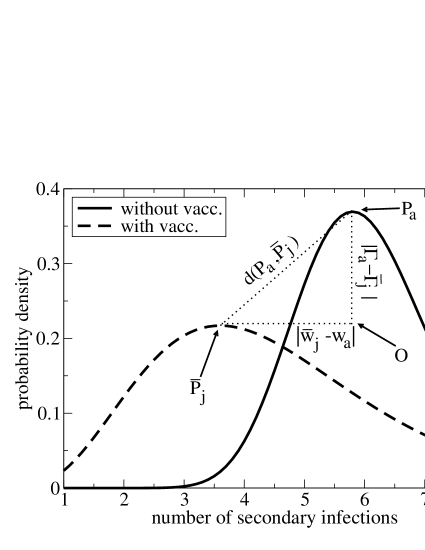
Figure 3.1. Examples of infection peaks with ($P_{j}$) and without ($P_{a}$) vaccination. For the with-vaccination scenario, the average peak over many possible types is shown (see text).

For $j$ possible types of post vaccine densities, let $\overline{P_{j}}(\overline{w_{j}},\Gamma(\overline{w_{j}}))$ be the point corresponding to the mean peak. $O$ is a point which is at a distance of $w_{a}-\overline{w_{j}}$ from $\overline{P_{j}}$ to the right. Suppose $\overline{d}(P_{a},\overline{P_{j}})$ is the distance from $P_{a}$ to $\overline{P_{j}}$. Then we know from Pythogoren right triangle principle that $d(P_{a},\overline{P_{j}})=\sqrt{(OP_{a})^{2}+(O\overline{P_{j}})^{2}}.$ From general principles of means, we can easily verify the fact that $d(P_{a},\overline{P_{j}})=\overline{d}(P_{j},P_{a}).$ Therefore,

$$\frac{1}{n^{2}}\left\{\sum_{j}d(P_{j},P_{a})\right\}^{2} = (w_{a}-\overline{w_{j}})^{2}+(\Gamma(w_{a})-\Gamma(\overline{w_{j}}))^{2}$$

$$\Gamma(\overline{w_{j}}) = \Gamma(w_{a})\pm\left[\frac{1}{n^{2}}\left\{\sum_{j}d(P_{j},P_{a})\right\}^{2}-(w_{a}-\overline{w_{j}})^{2}\right]^{\frac{1}{2}}$$

This proposition relates the shape of the distribution of the number of secondary infections per infected individual before vaccination to the same after vaccination. This may be useful in situations where both distributions have small skew and $w_{a}$, $w_{j}$ correspond to the expectation values of the distributions. ∎

Corollary 3.4.

Suppose $I_{a}(\sigma^{2})$ and $I_{j}(\sigma^{2})$ are variances of infections corresponding to the distributions $\{\theta_{n_{a}}\}$ and $\{_{\theta_{n_{j}}}\}.$ Then we have $I_{a}(\sigma^{2})-I_{j}(\sigma^{2})=$

$$\sum_{n_{a}}\left(n_{a}-I_{a}^{\prime}(1)\right)^{2}\Pr\left[N=n_{a}\right]-\sum_{n_{j}}\left(n_{j}-I_{j}^{\prime}(1)\right)^{2}\Pr\left[N=n_{j}\right]$$

$$= \sum_{n_{a}}n_{a}^{2}\Pr\left[N=n_{a}\right]+2\left\{\left(I_{j}^{\prime}(1)\right)^{2}-\left(I_{a}^{\prime}(1)\right)^{2}\right\}-\sum_{n_{j}}n_{j}^{2}\Pr\left[N=n_{j}\right]+$$

$$\qquad\qquad\qquad\qquad\qquad\qquad\qquad\qquad\left\{\left(I_{a}^{\prime}(1)\right)^{2}-\left(I_{j}^{\prime}(1)\right)^{2}\right\}$$

$$= \sum_{n_{a}}n_{a}^{2}\Pr\left[N=n_{a}\right]-\sum_{n_{j}}n_{j}^{2}\Pr\left[N=n_{j}\right]-2\left\{\left(I_{a}^{\prime}(1)\right)+\left(I_{j}^{\prime}(1)\right)\right\}\overline{d}_{\left|A\right|}+$$

$$\qquad\qquad\qquad\qquad\qquad\qquad\qquad\qquad\left\{\left(I_{a}^{\prime}(1)\right)+\left(I_{j}^{\prime}(1)\right)\right\}\overline{d}_{\left|A\right|}$$

$$= \sum_{n_{a}}n_{a}^{2}\Pr\left[N=n_{a}\right]-\sum_{n_{j}}n_{j}^{2}\Pr\left[N=n_{j}\right]-\left\{\left(I_{a}^{\prime}(1)\right)+\left(I_{j}^{\prime}(1)\right)\right\}\overline{d}_{\left|A\right|}$$

In the above $I_{a}^{\prime}(1)-I_{j}^{\prime}(1)=\overline{d}_{\left|A\right|}.$ The above relation indicates that difference between variability between infection process also depends upon the adjusted distance between the peaks described above. If the process is critical then the above difference is expressed as a straight combination of second central moments.

Remark 3.5.

$$\sum n_{a}\Pr[Z_{n_{a}}=0]\leq 1 \Rightarrow \sum n_{j}\Pr[Z_{n_{j}}=0]\leq 1$$

$$\Rightarrow\overline{d}(P_{j},P_{a}) \leq v^{2}\;\textrm{for some $v\leq 1$}$$

Again,

$$\sum n_{a}\Pr[Z_{n_{a}}=0]>1 \Rightarrow \left\{\begin{array}[]{c}\sum n_{j}\Pr[Z_{n_{j}}=0]>1\;(\textrm{no impact of vaccination})\\ \sum n_{a}\Pr[Z_{n_{a}}=0]\leq 1\;(\textrm{impact of vaccination})\end{array}\right.$$

Since vaccine has a positive role in reducing the infection process such that as $n_{j}>N$ (for some large $N$) it implies $\sum n_{j}\Pr[Z_{n_{j}}=0]\leq 1.$ When the process $\{Z_{n_{a}}\}$ is supercritical then initially the process $\{Z_{n_{j}}\}$ could also be supercritical and eventually $\{Z_{n_{j}}\}$ will attain sub criticality or criticality. Hence even if $\sum n_{a}\Pr[Z_{n_{a}}=0]>1$, eventually $d>1.$ The larger the value of $d$ the larger is the impact of vaccination and extinction occures much earlier with probability $\pi_{j}$$(\pi_{j}<\pi).$

4. Conclusions

Branching process analyses have provided a rigorous perspective on numerous physical problems in the past. Here, we have introduced the foundations for application of branching processes to studying the early stages of epidemic spread in a population, both with and without vaccination. We modified the standard branching process to account for the effects of vaccination, showing how vaccination will decrease the time to extinction. There remains much work to be done in epidemic branching processes, particularly in the incorporation of other types of control measures (quarantine) and in the incorporation of realistic population structures such as age-structure.

References

- [1] Jansen VAA, Stollenwerk N, Jensen HJ, et al. Measles outbreaks in a population with declining vaccine uptake. Science (2003) 301: 804-804
- [2] Feller, W. An introduction to probability theory and its applications. Vol. I. John Wiley & Sons, Inc., New York-London-Sydney 1968.
- [3] Alsmeyer, G; Rasler, U Asexual versus promiscuous bisexual Galton-Watson processes: the extinction probability ratio. Ann. Appl. Probab. 12 (2002), no. 1, 125–142.
- [4] Rao A.S.R.S. Probabilities of therapeutic extinction of HIV. Appl. Math. Lett. 19 (2006), no. 1, 80–86.
- [5] Broberg, Per A note on the extinction probability of branching populations. Scand. J. Statist. 14 (1987), no. 2, 125–129.
- [6] Allen, J.S.A. An Introduction to Stochactic Processes With Applications to Biology.
- [7] Jones, OD. On the convergence of multitype branching processes with varying environments. Ann. Appl. Probab. 7 (1997), no. 3, 772–801.
- [8] Jagers, P. Coupling and population dependence in branching processes. Ann. Appl. Probab. 7 (1997), no. 2, 281–298.
- [9] Schinazi, R.B. Classical and spatial stochastic processes. Birkhauser Boston, Inc., Boston, MA, 1999
- [10] Dwass, M. Branching processes in simple random walk. Proc. Amer. Math. Soc. 51 (1975), 270–274.
- [11] Athreya, Krishna B.; Ney, Peter E. Branching processes.Springer-Verlag, New York-Heidelberg, 1972
- [12] Bailey, NTJ. The elements of stochastic processes with applications to the natural sciences. John Wiley & Sons, Inc., New York-London-Sydney 1964.
- [13] Cohn, H. Multitype finite mean supercritical age-dependent branching processes. J. Appl. Probab. 26 (1989), no. 2, 398–403.
- [14] Grey, D. R. On regular branching processes with infinite mean. Stochastic Process. Appl. 8 (1978/79), no. 3, 257–267.
- [15] Williams, D. Probability with martingales. Cambridge University Press, Cambridge, 1991
- [16] Wei, C. Z.; Winnicki, J. Estimation of the means in the branching process with immigration. Ann. Statist. 18 (1990), no. 4, 1757–1773.