3D simulations of early blood vessel formation

Abstract

Blood vessel networks form by spontaneous aggregation of individual cells migrating toward vascularization sites (vasculogenesis). A successful theoretical model of two dimensional experimental vasculogenesis has been recently proposed, showing the relevance of percolation concepts and of cell cross-talk (chemotactic autocrine loop) to the understanding of this self-aggregation process. Here we study the natural 3D extension of the computational model proposed earlier, which is relevant for the investigation of the genuinely threedimensional process of vasculogenesis in vertebrate embryos. The computational model is based on a multidimensional Burgers equation coupled with a reaction diffusion equation for a chemotactic factor and a mass conservation law. The numerical approximation of the computational model is obtained by high order relaxed schemes. Space and time discretization are performed by using TVD schemes and, respectively, IMEX schemes. Due to the computational costs of realistic simulations, we have implemented the numerical algorithm on a cluster for parallel computation. Starting from initial conditions mimicking the experimentally observed ones, numerical simulations produce network-like structures qualitatively similar to those observed in the early stages of in vivo vasculogenesis. We develop the computation of critical percolative indices as a robust measure of the network geometry as a first step towards the comparison of computational and experimental data.

1 Introduction

In recent years, biologists have collected many qualitative and quantitative data on the behavior of microscopic components of living beings. We are, however, still far from understanding in detail how these microscopic components interact to build functions which are essential for life. A problem of particular interest which has been extensively investigated is the formation of patterns in biological tissues [2]. Such patterns often show self-similarity and scaling laws [18] similar to those emerging in the physics of phase transitions [26].

The vascular network [28, 29] is a typical example of natural structure characterized by non trivial scaling laws. In recent years many experimental investigations have been performed on the mechanism of blood vessel formation [6] both in living beings and in in vitro experiments. Vascular networks form by spontaneous aggregation of individual cells travelling toward vascularization sites (vasculogenesis). A successful theoretical model of two dimensional experimental vasculogenesis has been recently proposed, showing the relevance of percolation concepts and of cell cross-talk (chemotactic autocrine loop) to the understanding of this self-aggregation process.

Theoretical and computational modelling is useful in testing biological hypotheses in order to explain which kind of coordinated dynamics gives origin to the observed highly structured tissue patterns. One can develop computational models based on simple dynamical principles and test whether they are able to reproduce the experimentally observed features. If the basic dynamical principles are correctly chosen, computational experiments allow to observe the emergence of complex structures from a multiplicity of interactions following simple rules.

Apart from the purely theoretical interest, reproducing biological dynamics by computational models allows to identify those biochemical and biophysical parameters which are the most important in driving the process. This way, computational models can produce a deeper understanding of biological mechanisms, which in principle may end up having relevant practical consequences. It is worth noticing here that a complete understanding of the vascularization process is possible only if it is considered in its natural threedimensional setting ([1, 7]).

In this paper we illustrate computational results regarding the simulation of vascular network formation in a threedimensional environment. We consider the threedimensional version of the model proposed in [10, 23]. The model is based on a Burgers-like equation, a well studied paradigm in the theory of pattern formation, integrated with a feedback term describing the chemotactic autocrine loop. The numerical evolution of the computational model starting from initial conditions mimicking the experimentally observed ones produces network-like structures qualitatively similar to those observed in the early stages of in vivo vasculogenesis.

Since in the long run we are interested in developing quantitative comparison between experimental data and theoretical model, we start by selecting a set of observable quantities providing robust quantitative information on the network geometry. The lesson learned from the study of twodimensional vasculogenesis is that percolative exponents [27] are an interesting set of such observables, so we test the computation of percolative exponents on simulated network structures.

A thorough quantitative comparison of the geometrical properties of experimental and computational network structures will become possible as soon as an adequate amount of experimental data, allowing proper statistical computation, will become available.

The paper is organized as follows. Section 2 summarizes some background knowledge on the biological problem of vascular network formation. Section 3 is a short review of the properties of the model introduced in [10, 23]. In Section 4 the numerical approximation technique for the model is described. In Section 5 we describe the qualitative properties of simulated network structures and present the results of the computation of the exponents of the percolative transition. Finally, in the Conclusions, we point out at predictable developments of our research.

2 Biological background

To supply tissues with nutrients in an optimal way, vertebrates have developed a hierarchical vascular system which terminates in a network of size-invariant units, i.e. capillaries. Capillary networks characterized by intercapillary distances ranging from $50$ to $300\,\mu\mathrm{m}$ are essential for optimal metabolic exchange [11].

Capillaries are made of endothelial cells. Their growth is essentially driven by two processes: vasculogenesis and angiogenesis [6]. Vasculogenesis consists of local differentiation of precursor cells to endothelial ones, that assemble into a vascular network by directed migration and cohesion. Angiogenesis is essentially characterized by sprouting of novel structures and their remodelling.

In twodimensional assays, the process of formation of a vascular network starting from randomly seeded cells can be accurately tracked by videomicroscopy [10] and it is observed to proceed along three main stages: i) migration and early network formation, ii) network remodelling and iii) differentiation in tubular structures. During the first phase, which is the most important for determining the final geometrical properties of the structures, cells migrate over distances which are an order of magnitude larger than their radius and aggregate when they adhere with one of their neighbours. An accurate statistics of individual cells trajectories has been presented in [10], showing that, in the first stage of the dynamics, cell motion has marked directional persistence, pointing toward zones of higher cell concentration. This indicates that cells communicate through the emission of soluble chemical factors that diffuse (and degrade) in the surrounding medium, moving toward the gradients of this chemical field. Cells behave like not-directly interacting particles, the interaction being mediated by the release of soluble chemotactic factors. Their dynamics is well reproduced by the theoretical model proposed in [10].

The lessons learned from the study of in vitro vasculogenesis is thus that the formation of experimentally observed structures can be explained as the consequence of cell motility and of cell cross-talk mediated by the exchange of soluble chemical factors (chemotactic autocrine loop). The theoretical model also shows that the main factors determining the qualitative properties of the observed vascular structures are the available cell density and the diffusivity and half-life of the soluble chemical exchanged. It seems that only the dynamical rules followed by the individual cell are actually encoded in the genes. The interplay of these simple dynamical rules with the geometrical and physical properties of the environment produces the highly structured final result.

At the moment, no direct observation of the chemotactic autocrine loop regulating vascular network formation is available, although several indirect biochemical observations point to it, so, the main evidence in this sense still comes from the theoretical analysis of computational models.

Several major developments in threedimensional cell culture and in cell and tissue imaging allow today to observe in real time the mechanisms of cell migration and aggregation in threedimensional settings [9, 21].

In the embryo, endothelial cells are produced and migrate in a threedimensional scaffold, the extracellular matrix. Migration is actually performed through a series of biochemical processes, such as sensing of chemotactic gradients, and of mechanical operations, such as extensions, contractions, and degrading of the extracellular matrix along the way.

The evidence provided by twodimensional experimental vasculogenesis suggests that cell motion can be directed by an autocrine loop of soluble chemoattractant factors also in the real threedimensional environment.

As a sample of typical vascular structures that are observe in a threedimensional setting in the early stages of development of a living being, we include here $(750\,\mu\mathrm{m)^{2}}$ images of chick embryo brain at different development stages (Fig. 1). At an early stage (about 52-64 hours) one observes a typical immature vascular network formed by vasculogenesis and characterized by a high density of similar blood vessels (Fig. 1A). At the next stage (70-72 hours) we observe initial remodelling of the vascular network (Figs. 1B,C). Remodeling becomes more evident when the embryo is 5 days old, when blood vessels are organized in a mature, hierarchically organized vascular tree (Fig. 1D).

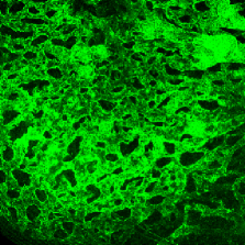
A B

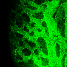
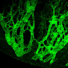
C D

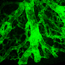
Figure 1: Vascular networks formed by vasculogenesis in chick embryo brain, at various stages of development, classified according to Hamilton and Hamburger (HH). A: HH stage 17, corresponding to 52-64 hours; B: HH stage 20 (70-72 hours); C,D: HH stage 26 (5 days).

3 Mathematical model of blood vessel growth

The multidimensional Burgers’ equation is a well-known paradigm in the study of pattern formation. It gives a coarse grained hydrodynamic description of the motion of independent agents performing rectilinear motion and interacting only at very short ranges. These equations have been utilized to describe the emergence of structured patterns in many different physical settings (see e.g. [24, 15]). In the early stages of dynamics, each particle moves with a constant velocity, given by a random statistical distribution. This motion gives rise to intersection of trajectories and formation of shock waves. After the birth of these local singularities regions of high density grow and form a peculiar network-like structure. The main feature of this structure is the existence of comparatively thin layers and filaments of high density that separate large low-density regions.

In order to study and identify the factors influencing blood vessel formation one has to take into account evidence suggesting that cells do not behave as independent agents, but rather exchange information in the form of soluble chemical factors. This leads to the model proposed by Gamba et al. in  [10] and Serini et al. in [23]. The model describes the motion of a fluid of randomly seeded independent particles which communicate through emission and absorption of a soluble factor and move toward its concentration gradients.

3.1 Model equations

The cell population is described by a continuous density $n(\mathbf{x},t)$, where $\mathbf{x}\in\mathbf{R}^{d}$ ($d=2,3$) is the space variable, and $t\geq 0$ is the time variable. The population density moves with velocities $\mathbf{v}(\mathbf{x},t)$, that are stimulated by chemical gradients of a soluble factor. The chemoattractant soluble factor is described by a scalar chemical concentration field $c(\mathbf{x},t)$. It is supposed to be released by the cells, diffuse, and degrade in a finite time, in agreement with experimental observations.

The dynamics of the cell density can be described by coupling three equations. The first one is the mass conservation law for cell matter, which expresses the conservation of the number of cells. The second one is a momentum balance law that takes into account the phenomenological chemotactic force, the dissipation by interaction with the substrate, the phenomenon of cell directional persistency along their trajectories and a term implementing an excluded volume constraint [10, 3]. Finally there is a reaction-diffusion equation for the production, degradation and diffusion of the concentration of the chemotactic factor. One then has the following system:

$$\frac{\partial n}{\partial t}+\nabla\cdot(n\mathbf{v})=0$$ (1a)

$$\frac{\partial\mathbf{v}}{\partial t}+\mathbf{v}\cdot\nabla\mathbf{v}=\mu(c)\nabla c-\nabla\phi(n)-\beta(c)\mathbf{v}$$ (1b)

$$\frac{\partial c}{\partial t}=D\mathrm{\Delta}c+\alpha(c)n-\frac{c}{\tau}$$ (1c)

where $\mu$ measures the cell response to the chemotactic factor, while $D$ and $\tau$ are respectively the diffusion coefficient and the characteristic degradation time of the soluble chemoattractant. The function $\alpha$ determines the rate of release of the chemical factor. The friction term $-\beta\mathbf{v}$ mimics the dissipative interaction of the cells with the extracellular matrix.

A simple model can be obtained by assuming that the cell sensitivity $\mu$, the rate of release of the chemoattractant $\alpha$ and the friction coefficient $\beta$ are constant. A more realistic description may be obtained including saturation effects as functional dependencies of the aforementioned coefficients on the concentration $c$.

The term $\nabla\phi(n)$ is a density dependent pressure term, where $\phi(n)$ is zero for low densities, and increases for densities above a suitable threshold. This pressure is a phenomenological term which models short range interaction between cells and the fact that cells do not interpenetrate.

We observe that, at low density $n$ and for small chemoattractive gradients, (1bb) is an inviscid Burgers’ equation for the velocity field $\mathbf{v}$ [5], coupled to the standard reaction-diffusion equation (1cc) and the mass conservaton law (1aa).

Since in the early stages of development almost all intraembryonic mesodermal tissues contain migrating endothelial precursors, we use initial conditions representing a randomly scattered distribution of cells, i.e., we throw an assigned number of cells in random positions inside the cubic box, with zero initial velocities and zero initial concentration of the soluble factor, with a single cell given initially by a Gaussian bump of width $\sigma$ of the order of the average cell radius ($\simeq 15\mu\mathrm{m})$ and unitary weight in the integrated cell density field $n$.

In order to model the fact that closely packed cells resist to compression, a phenomenological, density dependent, pressure $\nabla\phi(n)$ acting only when cells become close enough to each other is introduced. The potential $\phi$ has to be monotonically increasing and constant for $n<n_{0}$ where $n_{0}$ is the close-packing density. Our simulations suggest that the exact functional form of $\phi(n)$ is not relevant. For simplicity we choose

$$\phi(n)=\begin{cases}B_{p}(n-n_{0})^{C_{p}}&n>n_{0}\\ 0&n\leq n_{0}\end{cases}$$ (2)

3.2 Parameter values

Fourier analysis of Eq. (1c) with constant parameters and in the fast diffusion approximation $\partial c/\partial t=0$ suggests that starting from the aformentioned initial conditions, equation (1) should develop network patterns characterized by a typical length scale $r_{0}=\sqrt{D\tau}$, which is the effective range of the interaction mediated by soluble factors. As a matter of fact, Fourier components $\hat{c}_{k}$ of the chemical field are related to the Fourier components of the density field $\hat{n}_{k}$ by the relation

$$\hat{c}_{k}=\frac{\alpha\tau\hat{n}_{k}}{D\tau k^{2}+1}.$$

This means that in equation (1) wavelengths of the field $n$ of order $r_{0}$ are amplified, while wavelengths $\lambda\gg r_{0}$ or $\lambda\ll r_{0}$ are suppressed.

Initial conditions introduce in the problem a typical length scale given by the average cell-cell distance $L/\sqrt{N}$, where $L$ is the system size and $N$ the particle number. The dynamics, filtering wavelengths [8], rearranges the matter and forms a network characterized by the typical length scale $r_{0}$.

It is interesting to check the compatibility of the theoretical prediction with physical data. From available experimental results [22] it is known that the order of magnitude of the diffusion coefficient for major angiogenic growth factors is $D=10^{-7}\hskip 2.5pt\mathrm{cm}^{2}\hskip 2.5pt\mathrm{s}^{-1}$. In the experimental conditions that were considered in [10] the half life of soluble factors is $64\pm 7\hskip 2.5pt\mathrm{\min}$. This gives $r_{0}\sim 200\hskip 2.5pt\mu\mathrm{m}$, a value in good agreement with experimental observations.

3.3 Lower dimensional models

In order to get some intuition about the typical system dynamics, we exploit the 1D version of model (1) to simulate the “collision” of two cells. For small values of $B_{p}$ and sufficiently high $C_{p}$ in (2), the two bumps merge into a single one (see Fig. 2 left) which appears to be stationary, as suggested also by the graphs of the kinetic energy and of the momentum of inertia (Fig. 3 top). On the other hand a less smooth onset of pressure obtained with larger $B_{p}$ or smaller $C_{p}$ leads to forces overcoming the chemical attractive ones, making the two bumps bounce back (Fig. 2 right, Fig. 3 bottom). We observe that the better dynamics from the biological point of view is the first behavior with two bump coalescing.

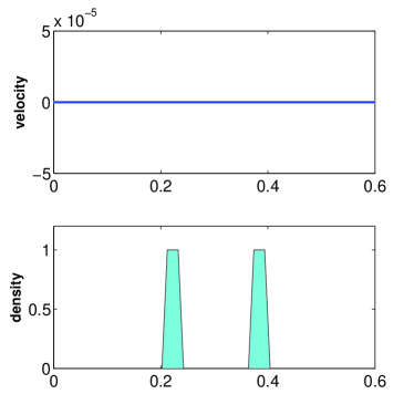
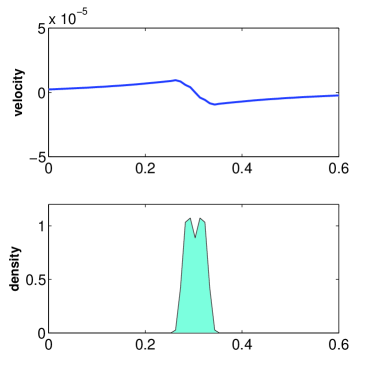
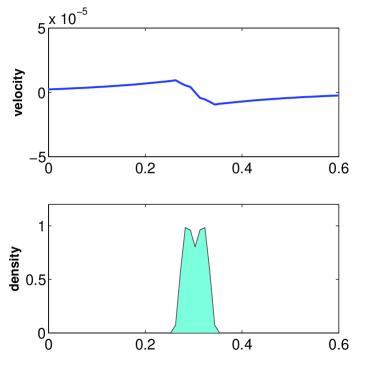
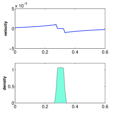
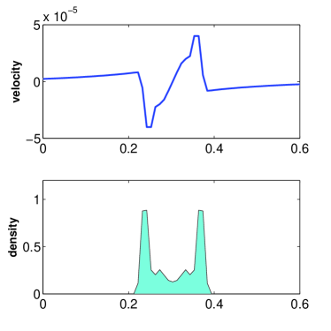
Figure 2: Bump coalescence driven by chemotactic force and pressure. In the first three rows the density and velocity fields at subsequent instants of time are shown. In the last row we show the time evolution of the kinetic energy and of the momentum of inertia. Left column: $C_{p}=3$ and $B_{p}=10^{-3}$, leading to bump coalescence. Right column: $C_{p}=2$ and $B_{p}=10^{-1}$, leading to undesired rebound of the two bumps.

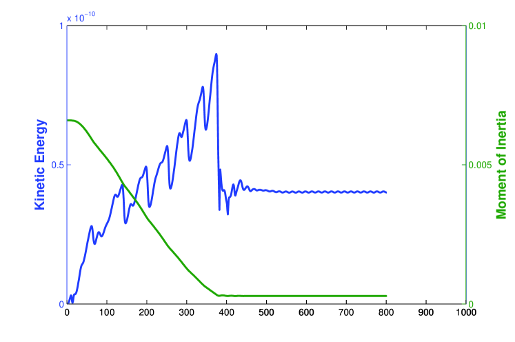
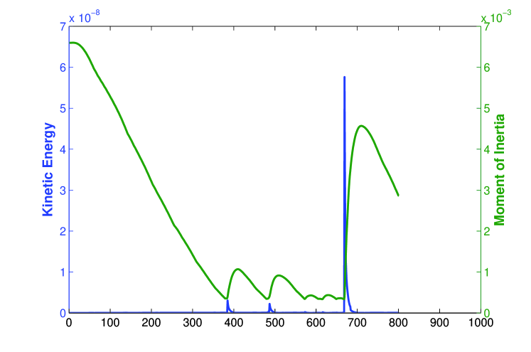
Figure 3: Time evolution of the kinetic energy and of the momentum of inertia. Top: $C_{p}=3$ and $B_{p}=10^{-3}$, leading to bump coalescence. Bottom: $C_{p}=2$ and $B_{p}=10^{-1}$, leading to undesired rebound of the two bumps.

Biological observations suggest that the dynamics of cell changes when they establish cell-cell contacts. It is reasonable to suppose that a different genetic program is activated at this moment, disabling cell motility. We therefore switch off cell motility as soon as the cell concentration, signalled by chemoattractant emission, reaches a given threshold. In this way the computational system is guaranteed to reach a stationary state.

These effects can be taken into account using a non-constant sensitivity $\mu(c)$, a non-linear emission rate $\alpha(c)$, or a variable friction coefficient $\beta(c)$. We choose a threshold $c_{0}$ and functions of the form

$$\mu(c) =\mu_{0}[1-\tanh(c-c_{0})]$$ (3a)

$$\alpha(c) =\alpha_{0}[1-\tanh(c-c_{0})]$$ (3b)

$$\beta(c) =\beta_{0}[1+\tanh(c-c_{0})]$$ (3c)

The effect of the first two terms is that the sensitivity of the cells and their chemoattractant production is strongly damped when the concentration $c$ reaches the threshold $c_{0}$. We did not observe a significant dependence on the exact form of the damping function, provided that it approximates a step function that is nonzero only when $c<c_{0}$.

$\beta(c)$, on the other hand has the effect of turning on a strong friction term at locations of high chemoattractant concentration. We performed several tests and observed that the different choices are approximately equivalent in freezing the system into a network-like stationary state.

4 Numerical methods

Our scheme is based on a suitable relaxation approximation [14] of the mass conservation law (1a) and the multidimensional Burgers equation (1b) coupled with a second order finite-differences method for the reaction-diffusion equation (1c) of the chemotactic factor. We point out that also for the last equation (1c) we could consider a relaxation approximation [13, 19] in order to deal with the system (1) in an uniform way, but we prefer to adopt here a simpler approach.

We first briefly review an extension of the approach proposed by Jin and Xin in [14] for a scalar conservation law to the case when a source term is present

$$\frac{\partial u}{\partial t}+\frac{\partial}{\partial x}f(u)=g(u).$$ (4)

Introducing an auxiliary variable $j$ that plays the role of a physical flux we consider the following relaxation system:

$$\frac{\partial u}{\partial t}+\frac{\partial j}{\partial x}=g(u)$$ (5a)

$$\frac{\partial j}{\partial t}+a\frac{\partial u}{\partial x}=-\frac{1}{\epsilon}(j-f(u)),$$ (5b)

where $\epsilon$ is a small positive parameter, called relaxation time, and $a$ is a suitable positive constant. Formally, Chapman-Enskog expansion justifies the agreement of the solutions of the relaxation system with the solutions of the equation

$$\frac{\partial u}{\partial t}+\frac{\partial}{\partial x}f(u)=g(u)+\epsilon\frac{\partial}{\partial x}\left((a-f^{\prime}(u)^{2})\frac{\partial u}{\partial x}\right),$$ (6)

which is a first order approximation of the original balance law (4).

It is also clear that (6) is dissipative, provided that the subcharacteristic condition $a>f^{\prime}(u)^{2}$ is satisfied. We would expect that appropriate numerical discretization of the relaxation system (5) yields accurate approximation to the original equation (4) when the relaxation parameter $\epsilon$ is sufficiently small.

In view of its numerical approximation, the main advantage of the relaxation system (5) over the original equation (4) lies in the linear structure of the characteristic fields and in the localized low order term and this avoids the use of time consuming Riemann solvers. Moreover, proper implicit time discretization can be exploited to overcome the stability constraints due to the stiffness and to avoid the use of non-linear solvers.

We observe that system (5) is in the form

$$\frac{\partial{z}}{\partial{t}}+\mathrm{div}f(z)=g(z)+\frac{1}{\epsilon}h(z)$$ (7)

where $z=(u,j)^{T}$, $f(z)=(j,au)^{T}$, $g(z)=(g(u),0)^{T}$ and $h(z)=(0,j-f(u))^{T}$. When $\varepsilon$ is small, the presence of both non-stiff and stiff terms, suggests the use of IMEX schemes [4, 16, 20].

Assume for simplicity to adopt a uniform time step $\Delta t$ and denote with $z^{n}$ the numerical approximation at time $t_{n}=n\Delta t$, for $n=0,1,\ldots$ In our case a $\nu$-stages IMEX scheme reads

$$z^{n+1}=z^{n}-\Delta t\sum_{i=1}^{\nu}\tilde{b}_{i}\left[\frac{\partial{f}}{\partial{x}}(z^{(i)})+g(z^{(i)})\right]+\frac{\Delta t}{\varepsilon}\sum_{i=1}^{\nu}b_{i}h(z^{(i)})$$

where the stage values are computed as

$$z^{(i)}=z^{n}-\Delta t\sum_{k=1}^{i-1}\tilde{a}_{i,k}\left[\frac{\partial{f}}{\partial{x}}(z^{(k)})+g(z^{(k)})\right]+\frac{\Delta t}{\varepsilon}\sum_{k=1}^{i}a_{i,k}h(z^{(k)})$$

Here $({a}_{ik},{b}_{i})$ and $(\tilde{a}_{ik},\tilde{b}_{i})$ are a pair of Butcher’s tableaux of, respectively, a diagonally implicit and an explicit Runge-Kutta schemes.

In this work we use the so-called relaxed schemes, that are obtained letting $\varepsilon\rightarrow 0$ in the numerical scheme for (7). For these the first stage

$$\left[\begin{array}[]{l}{u^{(1)}}\\ {j^{(1)}}\end{array}\right]=\left[\begin{array}[]{l}u^{n}\\ j^{n}\end{array}\right]+\frac{\Delta t}{\varepsilon}a_{1,1}h\left(\left[\begin{array}[]{l}u^{(1)}\\ j^{(1)}\end{array}\right]\right)$$

becomes

$${u^{(1)}=u^{n}}\qquad{j^{(1)}=f(u^{(1)})},$$

then it reduces to $h(z^{(1)})=0$. While the second stage, $i=2$, reads

$$z^{(2)}=z^{n}-\Delta{t}\tilde{a}_{2,1}{\left[\frac{\partial{f}}{\partial{x}}(z^{(1)})+g(z^{(1)})\right]}+\frac{\Delta t}{\varepsilon}a_{2,1}\underbrace{{h(z^{(1)})}}_{{\equiv 0}}+\frac{\Delta t}{\varepsilon}a_{2,2}{h(z^{(2)})}$$

which implies that $h(z^{(2)})=0$.

Summarizing, the relaxed scheme yields an alternation of relaxation steps

$$h(z^{(i)})=0\qquad\text{ i.e. }\,{j^{(i)}=f(u^{(i)})}$$

and transport steps where we advance for time $\tilde{a}_{i,k}\Delta{t}$

$$\frac{\partial{z}}{\partial{t}}+\mathrm{div}f(z)=g(z)$$

with initial data $z=z^{(i)}$ retain only the first component and assign it to $u^{(i+1)}$.

Finally the value of $u^{n+1}$ is computed as $u^{n}+\sum\tilde{b}_{i}u^{(i)}$.

In order to obtain a relaxation approximation of the first and second equation of (1) we rewrite them in conservative form, introducing the moment $\mathbf{p}(\mathbf{x},t)=n(\mathbf{x},t)\mathbf{v}(\mathbf{x},t)$:

$$\frac{\partial n}{\partial t}+\nabla\cdot\mathbf{p}=0$$ (8a)

$$\frac{\partial\mathbf{p}}{\partial t}+\nabla\cdot\left(\mathbf{n}\mathbf{v}\otimes\mathbf{v}\right)=n\mu\nabla c-n\nabla\phi(n)-\beta\mathbf{p}$$ (8b)

Introducing the variable $\mathbf{u}=(n,\mathbf{p})^{T}$ and the auxiliary flux $\mathbf{w}$, the relaxation system reads

$$\frac{\partial\mathbf{u}}{\partial t}+\nabla\cdot\mathbf{w}=G(\mathbf{u},\mathbf{w},c)$$ (9a)

$$\frac{\partial\mathbf{w}}{\partial t}+A\nabla\cdot\mathbf{u}=-\frac{1}{\varepsilon}\left(\mathbf{w}-F(\mathbf{u})\right)$$ (9b)

where $G(\mathbf{u},\mathbf{w},c)=(0,n\mu\nabla c-n\nabla\phi(n)-\beta\mathbf{p})^{T}$, $F(\mathbf{u})=(\mathbf{p},\mathbf{n}\mathbf{v}\otimes\mathbf{v})$ and $A$ is a suitable diagonal matrix whose positive diagonal elements verify a subcharacteristic condition. As we previously remarked, our relaxed scheme takes alternatively an implicit step and an explicit one: the explicit step involves the computation of the flux $\nabla\cdot\mathbf{w}$ and the evaluation of the non stiff source term $G$. In particular we compute $\nabla c$ and $\nabla\phi(n)$ using a second order difference scheme.

In the following we describe for simplicity the fully discrete scheme in one dimensional case. We introduce the spatial grid points $x_{j}$ with uniform mesh width $h=x_{j+1}-x_{j}$. As usual, we denote by $u_{j}^{n}$ the approximate cell average of a quantity $u$ in the cell $[x_{j-1/2},x_{j+1/2}]$ at time $t_{n}$ and by $u_{j+1/2}^{n}$ the approximate point value of $u$ at $x=x_{j+1/2}$ and $t=t_{n}$. A spatial discretization to (9) in conservation form can be written as

$$\frac{\partial\mathbf{u}_{j}}{\partial t}+\frac{1}{h}\left(\mathbf{w}_{j+1/2}-\mathbf{w}_{j-1/2}\right)=G(\mathbf{u}_{j},\mathbf{w}_{j},c_{j})$$ (10a)

$$\frac{\partial\mathbf{w}_{j}}{\partial t}+\frac{1}{h}A\left(\mathbf{u}_{j+1/2}-\mathbf{u}_{j-1/2}\right)=-\frac{1}{\varepsilon}\left(\mathbf{w}_{j}-F(\mathbf{u}_{j})\right).$$ (10b)

In order to compute the numerical fluxes $\mathbf{w}_{j\pm 1/2}$, we consider the characteristic variables $\mathbf{w}\pm A^{1/2}\mathbf{u}$ that travel with constant velocities $\pm A^{1/2}$, and so the semidiscrete system becomes diagonal. Now we have to apply a numerical approximation to $\mathbf{w}\pm A^{1/2}\mathbf{u}$. A first idea is to apply a ENO or WENO approach (see e.g. [25]), to build an high order reconstruction, coupled with a suitable IMEX scheme. The drawback is the high computational costs, especially in a multidimensional framework. Therefore we chose a suitable compromise between the computational cost and the accuracy, using a second order TVD scheme. The numerical flux that we use is obtained coupling an upwind scheme and the Lax-Wendroff method by a non linear flux limiter [17]. Namely the high order flux $F(U)$ for a generic variable $U$ consists of the low order term $F_{L}(U)$ plus a second order correction $F_{H}(U)$:

$$F(U)=F_{L}(U)+\Psi(U)(F_{H}(U)-F_{L}(U))$$

where $\Psi$ is the flux limiter. When the data $U$ is smooth, then $\Psi(U)$ should be near $1$, while near a discontinuity we want $\Psi(U)$ close to $0$. The idea consists in the selection of a high order flux $F_{H}$ that works well in smooth regions and of a low order flux $F_{L}$ which behaves well near discontinuities.

In our schemes we considered the upwind scheme as a low order flux for the characteristic variables

$$F_{L}((\mathbf{w}+A^{1/2}\mathbf{u})_{j+1/2})=(\mathbf{w}+A^{1/2}\mathbf{u})_{j},\quad F_{L}((\mathbf{w}-A^{1/2}\mathbf{u})_{j+1/2})=(\mathbf{w}-A^{1/2}\mathbf{u})_{j+1}$$

and the Lax-Wendroff scheme as a high order flux for the same variables

$$\begin{array}[]{ll}F_{H}((\mathbf{w}\pm A^{1/2}\mathbf{u})_{j+1/2})=&\frac{A^{1/2}}{2}((\mathbf{w}\pm A^{1/2}\mathbf{u})_{j+1}+(\mathbf{w}\pm A^{1/2}\mathbf{u})_{j})\\ &-\frac{\lambda A^{1/2}}{2}((\mathbf{w}\pm A^{1/2}\mathbf{u})_{j+1}-(\mathbf{w}\pm A^{1/2}\mathbf{u})_{j})\end{array}$$

where $\lambda=\Delta t/h$ (we advance of one time step).

Letting

$$\mathbf{\Theta}_{j}^{\pm}=\left(\frac{(\mathbf{w}\pm A^{1/2}\mathbf{u})_{j}^{n}-(\mathbf{w}\pm A^{1/2}\mathbf{u})_{j-1}^{n}}{(\mathbf{w}\pm A^{1/2}\mathbf{u})_{j+1}^{n}-(\mathbf{w}\pm A^{1/2}\mathbf{u})_{j}^{n}}\right)^{\pm 1}\,,$$

the fully discrete scheme for the variable $\mathbf{u}$ using Euler method to advance in time is the following

$$\begin{array}[]{ll}\mathbf{u}_{j}^{n+1}=&\mathbf{u}_{j}^{n}+\frac{\lambda A^{1/2}}{2}(\mathbf{u}_{j+1}^{n}-2\mathbf{u}_{j}^{n}+\mathbf{u}_{j-1}^{n})-\frac{\lambda}{2}(\mathbf{w}_{j+1}^{n}-\mathbf{w}_{j-1}^{n})\\ &\Delta t\frac{\mathbb{I}-\lambda A^{1/2}}{4}(-s_{j}^{+}+s_{j-1}^{+}+s_{j+1}^{-}-s_{j}^{-}),\end{array}$$

with

$$s_{j}^{\pm}=\frac{1}{h}(\pm A^{1/2}\mathbf{u}_{j\pm 1}^{n}+\mathbf{w}_{j\pm 1}^{n}\mp A^{1/2}\mathbf{u}_{j}^{n}-\mathbf{w}_{j}^{n})\Psi(\Theta_{j}^{\pm}).$$ (11)

After the substitution of the relaxing step we get

$$\begin{array}[]{ll}\displaystyle\mathbf{u}_{j}^{n+1}=&\mathbf{u}_{j}^{n}+\frac{\lambda A^{1/2}}{2}(\mathbf{u}_{j+1}^{n}-2\mathbf{u}_{j}^{n}+\mathbf{u}_{j-1}^{n})-\frac{\lambda}{2}(F(\mathbf{u}_{j+1}^{n})-F(\mathbf{u}_{j+1}^{n}))\\ \displaystyle&\Delta t\frac{\mathbb{I}-\lambda A^{1/2}}{4}(-s_{j}^{+}+s_{j-1}^{+}+s_{j+1}^{-}-s_{j}^{-}),\end{array}$$

where $s^{\pm}$ is obtained from (11) letting $\mathbf{w}=F(\mathbf{u})$. The scheme can be put in a conservative form and it is possible to prove its consistency by standard technique [17]. In order to prove a TVD stability, we write

$$\begin{array}[]{ll}\displaystyle\mathbf{u}_{j+1}^{n+1}-\mathbf{u}_{j}^{n+1}=&(1-\mathbf{C}_{j}^{n}-\mathbf{D}_{j}^{n})(\mathbf{u}_{j+1}^{n}-\mathbf{u}_{j}^{n})+\mathbf{C}_{j-1}^{n}(\mathbf{u}_{j}^{n}-\mathbf{u}_{j-1}^{n})\\ \displaystyle&+\mathbf{D}_{j+1}^{n}(\mathbf{u}_{j+2}^{n}-\mathbf{u}_{j+1}^{n})+E_{j+1/2},\end{array}$$ (12)

where

$$\begin{array}[]{lll}\displaystyle\mathbf{C}_{j}^{n}&=&\frac{\lambda}{2}\left(A^{1/2}+\frac{F(\mathbf{u}_{j+1}^{n})-F(\mathbf{u}_{j}^{n})}{\mathbf{u}_{j+1}^{n}-\mathbf{u}_{j}^{n}}\right)\\ \displaystyle\mathbf{D}_{j}^{n}&=&\frac{\lambda}{2}\left(A^{1/2}-\frac{F(\mathbf{u}_{j+1}^{n})-F(\mathbf{u}_{j}^{n})}{\mathbf{u}_{j+1}^{n}-\mathbf{u}_{j}^{n}}\right)\\ \displaystyle E_{j+1/2}^{n}&=&\Delta t\frac{1-\lambda A^{1/2}}{4}\left(s_{j+2}^{-}-2s_{j+1}^{-}+s_{j}^{-}-s_{j+1}^{+}+2s_{j}^{+}-s_{j-1}^{+}\right)\end{array}$$

where we notice that $\mathbf{C}$ and $\mathbf{D}$ are non negative.

The coefficient $E$ can be written in terms of $\mathbf{C}$ and $\mathbf{D}$, in fact

$$s_{j}^{+}=\frac{2}{\lambda\Delta x}\mathbf{C}_{i}^{n}\Psi(\mathbf{\Theta}_{i}^{+})(\mathbf{u}_{j+1}^{n}-\mathbf{u}_{j}^{n})),\quad s_{j}^{-}=-\frac{2}{\lambda\Delta x}\mathbf{D}_{i-1}^{n}\Psi(\mathbf{\Theta}_{i}^{-})(\mathbf{u}_{j}^{n}-\mathbf{u}_{j-1}^{n})).$$

We can rewrite (12) in the following form

$$\begin{array}[]{ll}\displaystyle\mathbf{u}_{j+1}^{n+1}-\mathbf{u}_{j}^{n+1}=&(\mathbf{u}_{j+1}^{n}-\mathbf{u}_{j}^{n})\left[(1-\mathbf{C}_{j}^{n}-\mathbf{D}_{j}^{n})+(1-\lambda A^{1/2})(\mathbf{D}_{j}^{n}\Psi_{j+1}^{-}+\mathbf{C}_{j}^{n}\Psi_{j}^{+})\right]\\ &+(\mathbf{u}_{j}^{n}-\mathbf{u}_{j-1}^{n})\left[\mathbf{C}_{j-1}^{n}-\frac{1-\lambda A^{1/2}}{2}(\mathbf{D}_{j-1}^{n}\Psi_{j}^{-}+\mathbf{C}_{j-1}^{n}\Psi_{j-1}^{+})\right]\\ &+(\mathbf{u}_{j+2}^{n}-\mathbf{u}_{j+1}^{n})\left[\mathbf{D}_{j+1}^{n}-\frac{1-\lambda A^{1/2}}{2}(\mathbf{D}_{j+1}^{n}\Psi_{j+2}^{-}+\mathbf{C}_{j+1}^{n}\Psi_{j+1}^{+})\right]\end{array}$$ (13)

It’s easy to see that under the CFL condition $\|\lambda\sqrt{\max\{a_{i}\}}\|\leq 1$, where $a_{i}$ are the positive diagonal elements of the matrix $A$, and using the fact that the flux limiter verifies

$$0\leq\frac{\Psi(\mathbf{\Theta})}{\mathbf{\Theta}}\leq 2,\qquad 0\leq\Psi(\mathbf{\Theta})\leq 2,$$

we have

$$\begin{array}[]{rrr}(1-\mathbf{C}_{j}^{n}-\mathbf{D}_{j}^{n})+(1-\lambda A^{1/2})(\mathbf{D}_{j}^{n}\Psi_{j+1}^{-}+\mathbf{C}_{j}^{n}\Psi_{j}^{+})&\geq&0\\ \mathbf{C}_{j-1}^{n}-\frac{1-\lambda A^{1/2}}{2}(\mathbf{D}_{j-1}^{n}\Psi_{j}^{-}+\mathbf{C}_{j-1}^{n}\Psi_{j-1}^{+})&\geq&0\\ \mathbf{D}_{j+1}^{n}-\frac{1-\lambda A^{1/2}}{2}(\mathbf{D}_{j+1}^{n}\Psi_{j+2}^{-}+\mathbf{C}_{j+1}^{n}\Psi_{j+1}^{+})&\geq&0\end{array}$$

and so we can deduce that our scheme is TVD stable from Harten’s Theorem [12].

In the case of multidimensions, a similar discretization can be applied to each space dimension [14, 13, 19]. Then, since the structure of the multidimensional relaxation system is similar to the 1D system, the numerical implementation for higher dimensional problems, based on additive dimensional splitting, is not much harder than for 1D problems.

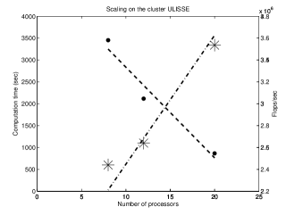
Figure 4: Scaling of the 3D algorithm on the ULISSE cluster. Dots represent execution time (s) and asterisks the number of Mflops/s for our numerical algorithm. Dashed and dash-dot lines are linear interpolations

For our threedimensional problem the computational cost is quite high and can be reduced using parallel computing: the semilinearity of relaxation systems, together with our suitably chosen discretizations, provides parallel algorithm with almost optimal scaling properties. In particular the domain is divided in smaller subdomains and each subdomain is assigned to a processor. The computations of all non linear terms involve only pointwise evaluations and it is easy to perform these tasks in a local way. Only point near the interfaces between different subdomain need to be communicated in the transport step. We implemented these algorithm on a high performance cluster for parallel computation installed at the Department of Mathematics of the University of Milano (http://cluster.mat.unimi.it/). The scaling properties of the algorithm are shown in Fig. 4 and are essentially due to the exclusive use of matrix-vectors operations and to the avoidance of solvers for linear or non-linear systems.

5 Numerical results

We perform threedimensional numerical simulations of model (1) on a cubic box with side of length $L=1\mathrm{mm}$, with periodic boundary conditions. The initial condition is assigned in the form of a set of gaussian bumps with $\sigma=15\mathrm{\mu{m}}$ scattered in the cube with uniform probability and having zero initial velocity.

Biochemical data [23] suggest the values $D=10^{-3}\mathrm{mm^{2}/s}$ and $\tau=4000\leavevmode\nobreak\ \mathrm{s}$ for the diffusion constant and the chemoattractant decay rate. We fix the other constant parameters by dimensional analysis and fitting to the characteristic scales of the biological system. In particular, we choose: $\mu_{0}=10^{-11}\mathrm{mm}^{4}/\mathrm{s}^{3}$, $\alpha=1\mathrm{s}^{-1}$, $\beta=10^{-3}\mathrm{s}^{-1}$. For the coefficients in the expression (2) of the pressure function $\phi$ we take $n_{0}=1.0$,$C_{p}=3$ and $B_{p}=10^{-3}$.

Very fine grids have to be used in order to resolve the details of the $n(\mathbf{x},t)$ field, which may contain hundreds of small bumps, each representing a single cell. Since each cell has radius $\sigma=15\mathrm{\mu m}$, one needs a grid spacing such that $\mathrm{\Delta{x}}<10\mathrm{\mu m}$ and therefore grids of at least $100^{3}$ cells for a cubic domain of $1\mathrm{mm}$ side.

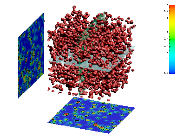
Figure 5: Initial state of a numerical simulation with $2500\mathrm{cells/mm}^{3}$. The colorbar on the right is referred to the coloring of the cross sections. The red three-dimensional isosurface corresponds to the black contour lines in the cross sections

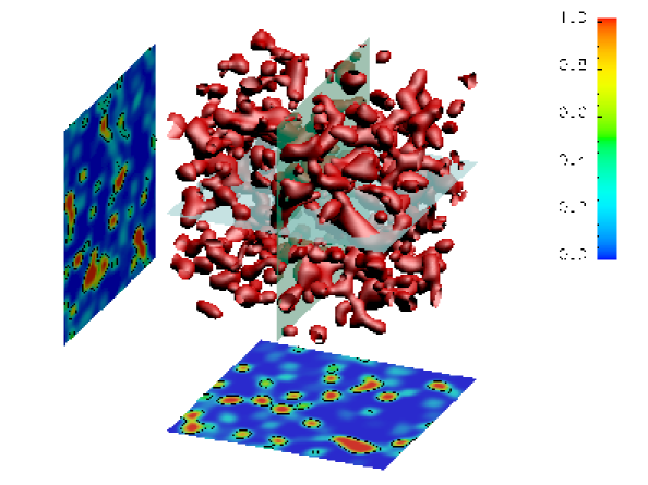
Figure 6: Transient state of the evolution of the initial state depicted in Fig. 5 according to model (1). The initial formation of network-like structures is observed

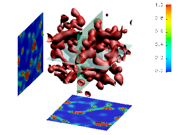
Figure 7: Stationary state of the evolution of the states depicted in Figs. 5 and 6 according to model (1). Well developed threedimensional network-like structures are observed

We performed numerical simulations with varying initial average cell density $\bar{n}$. We observed that the initially randomly distributed cells coalesce forming elongated structures and evolve towards a stationary state mimicking the geometry of a blood vessel network in the early stages of formation.

We assigned $\bar{n}$ in the range $2100-3500\,\mathrm{cells/mm^{3}}$ and performed 10 to 15 runs for each density value with a $128\times 128\times 128$ grid on a biological system of $1\leavevmode\nobreak\ \mathrm{mm}^{3}$. The characteristic lengths and geometric properties of the stationary state depend on $\bar{n}$ and we observed a percolative phase transition similar to the one described in [10] for the twodimensional case.

5.1 Analysis of the percolative phase transition

In experimental blood vessel formation it has been shown that a percolative transition is observed, by varying the initial cell density. For low cell densities only isolated clusters of endothelial cells are observed, while for very high densities cells fill the whole available space. In between these two extreme behaviours, close to a critical cell density $n_{c}$, one observes the formation of critical percolating clusters connecting opposite sides of the domain, characterized by well defined scaling laws and exponents. These exponents are known not to depend on the microscopic details of the process while their values characterize different classes of aggregation dynamics.

The purely geometric problem of percolation is actually one of the simplest phase transitions occurring in nature. Many percolative models show a second order phase transition in correspondence to a critical value $n_{\mathrm{c}}$, i.e. the probability $\Pi$ of observing an infinite, percolating cluster is $0$ for $\bar{n}<n_{\mathrm{c}}$ and $1$ for $\bar{n}>n_{\mathrm{c}}$ [27]. The phase transition can be studied by focusing on the values of an order parameter, i.e. an observable quantity that is zero before the transition and takes on values of order $1$ after it. In a percolation problem the natural order parameter is the probability $P$ that a randomly chosen site belongs to the infinite cluster (on finite grids, the infinite cluster is substituted by the largest one).

In the vicinity of the critical density $n_{c}$ the geometric properties of clusters show a peculiar scaling behavior. For instance, in a system of linear finite size $L$, the probability of percolation $\Pi(n,L)$, defined empirically as the fraction of computational experiments that produce a percolating cluster, is actually a function of the combination $(n-n_{\mathrm{{c}}})\,L^{1/\nu}$, where $\nu$ is a universal exponent.

In a neighborhood of the critical point and on a system of finite size $L$, the following finite size scaling relations are also observed:

$$\Pi(\bar{n},L)\>\sim\>\widehat{\Pi}[(\bar{n}-n_{\mathrm{c}})L^{1/\nu}]$$ (14)

There are two main reasons to study percolation in relation to vascular network formation: (i) percolation is a fundamental property for vascular networks: blood should have the possibility to travel through the whole vascular network to carry nutrients to tissues; (ii) critical exponents are robust observables characterizing the aggregation dynamics.

A rather complete characterization of percolative exponents in the two-dimensional case has been provided in [10].

As a first step in the study of the more realistic threedimensional case, we compute the exponent $\nu$ characterizing the structures produced by the model dynamics (1) with varying initial cell density.

To this aim, extensive numerical simulation of system (1) were performed using lattice sizes $L=1,0.78,0.62,0.5\,\mathrm{mm}$, with different values of the initial density $\bar{n}$. For each point 10 to 15 realizations of the system of size $1\mathrm{mm}$ were computed, depending on the proximity to the critical point.

The continuous density at final time $n(\mathbf{x})$ was then mapped to a set of occupied and empty sites by choosing a threshold $n_{0}$. Each region of adjacent occupied sites (cluster) was marked with a different index. The percolation probability $\Pi$ for each set of realizations was then measured. In Fig. 8 we show clusters obtained in a box with $L=0.5\,\mathrm{mm}$ with $\bar{n}=3100$. The largest percolating cluster is shown in red, together with some other smaller clusters shown in different colors.

Using relation (14), we estimate the position of the critical point $n_{\mathrm{c}}$ and the value of the critical exponent $\nu$. The data for different box side length and initial density should lie on a single curve after rescaling the densities as $\hat{n}=(\bar{n}-n_{c})L^{1/\nu}$. For fixed $n_{\mathrm{c}}$ and $\nu$ we rescale $\bar{n}$ and fit the data with a logistic curve, then compute the distance of the data from the curve. The squared distance is minimized to obtain estimates for $n_{\mathrm{c}}$ and $\nu$.

Using $n_{0}=0.35$ we obtain $n_{\mathrm{c}}=2658$ and $\nu=0.84$. This latter value is compatible with the known value $0.88$ for random percolation in three dimensions [27].

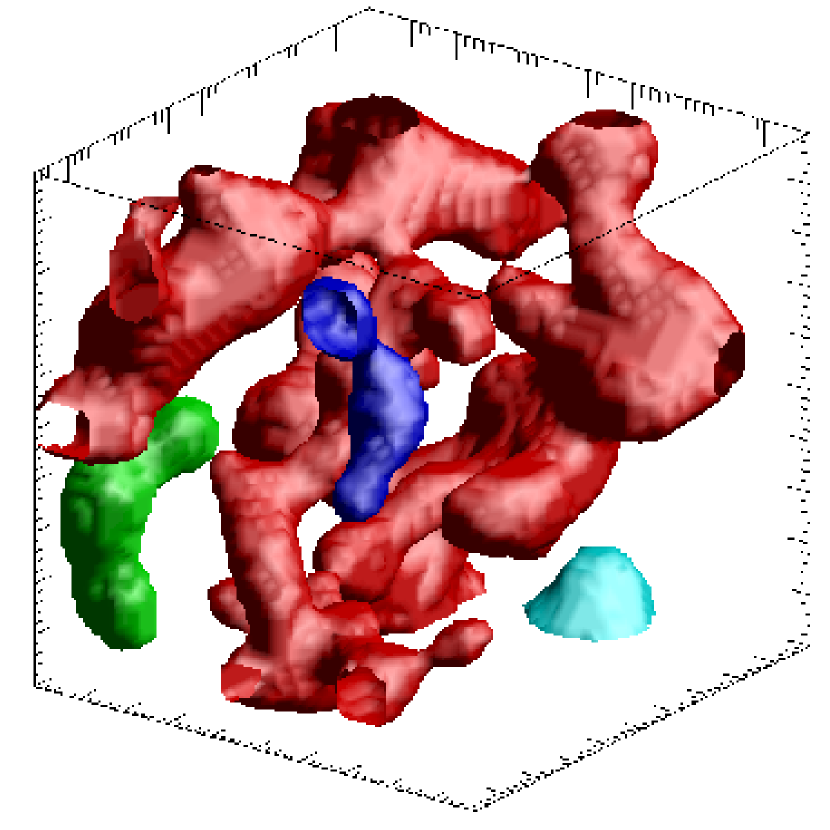
Figure 8: Cluster percolation with cell density $n=2500$cells/mm³. A: connected clusters in a realization of model (1). B: the largest cluster depicted in A percolates.

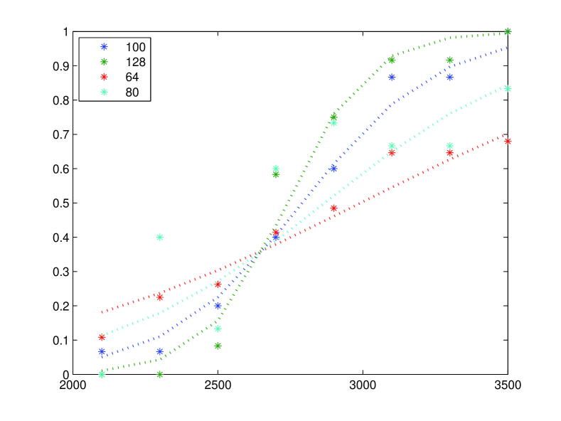
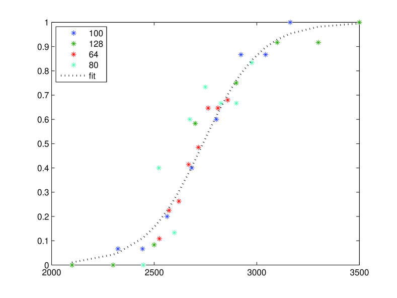
Figure 9: Percolation probability at varying densities A: B: the curves in A are collapsed according to formula (14)

6 Conclusions

We have exposed results on the numerical simulation of vascular network formation in a threedimensional setting.

We have used the threedimensional version of the equations proposed in [10, 23] as a computational model. Evolution starting from initial conditions mimicking the experimentally observed ones produce network-like structures qualitatively similar to those observed in the early stages of in vivo vasculogenesis.

As a starting point towards a quantitative comparison between experimental data and the theoretical model we nedd to select a set of observable quantitaties which provide robust quantitative information on the network geometry. The lesson learned from the study of twodimensional vasculogenesis is that percolative exponents are an interesting set of such observables, so we tested the computation of percolative exponents on simulated network structures.

A quantitative comparison of the geometrical properties of experimental and computational network structures will become possible as soon as an adequate amount of experimental data, allowing proper statistical computation, will become available.

In order to compute the robust statistical observables described in the paper one has to perform many runs of the simulation code using different random initial data. This, toghether with the intensive use of computational resources required by a three-dimensional hydrodynamic simulation on fine grids, calls for an efficient implementation of the computational model on parallel computers, as the one we presented in this paper.

Simulations of blood vessel structures can in principle present practical implications. Normal tissue function depends on adequate supply of oxygen through blood vessels. Understanding the mechanisms of formation of blood vessels has become a principal objective of medical research, because it would offer the possibility of testing medical treatments in silicio. One can think that the dynamical model (1) can be also exploited in the future to design properly vascularized artificial tissues by controlling the vascularization process through appropriate signaling patterns.

References

- [1] A. Abbott. Cell culture: biology’s new dimension. Nature, 424(6951):870–2, 2003.
- [2] A.J. Koch and H. Meinhardt. Biological pattern formation: from basic mechanisms to complex structures. Rev Mod Phys, 66(1481–1510), 1994.
- [3] D. Ambrosi, A. Gamba, and G. Serini. Cell directional persistence and chemotaxis in vascular morphogenesis. Bull. Math. Biol., 66(6):1851–73, 2004.
- [4] U. Asher, S. Ruuth, and R.J. Spiteri. Implicit-explicit Runge-Kutta methods for time dependent Partial Differential Equations. Appl. Numer. Math., 25:151–167, 1997.
- [5] J. Burgers. The non linear diffusion equation. D. Reidel Publ. Co., 1974.
- [6] P. Carmeliet. Mechanisms of angiogenesis and arteriogenesis. Nature Medicine, 6:389–395, 2000.
- [7] E. Cukierman, R. Pankov, D.R. Stevens, and K.M. Yamada. Taking cell-matrix adhesions to the third dimension. Science, 294(5547):1708–12, 2001.
- [8] S. Di Talia, A Gamba, F. Lamberti, and G. Serini. Role of repulsing factors in vascularization dynamics. Phys. Rev. E, 73:041917–1–11, 2006.
- [9] P. Friedl. Dynamic imaging of the immune system. Curr Opin Immunol, 16(4):389–93, 2004.
- [10] A. Gamba, D. Ambrosi, A. Coniglio, A. de Candia, S. Di Talia, E. Giraudo, G. Serini, L. Preziosi, and F. Bussolino. Percolation, morphogenesis, and Burgers dynamics in blood vessels formation. Phys. Rev. Lett., 90:118101, 2003.
- [11] A.C. Guyton and J.E. Hall. Textbook of medical physiology. W.B. Saunders, St. Louis, 2000.
- [12] Ami Harten. On a class of high resolution total-variation-stable finite difference schemes. SIAM J. Numer. Anal, 21(1):1–23, 1984.
- [13] S. Jin, L. Pareschi, and G. Toscani. Diffusive relaxation schemes for multiscale discrete-velocity kinetic equations. SIAM J. Numer. Anal., 35:2405, 1998.
- [14] S. Jin and Z. Xin. The relaxation schemes for systems of conservation laws in arbitrary space dimension. Comm. Pure and Appl. Math., 48:235–276, 1995.
- [15] M. Kardar, G. Parisi, and Y.C. Zhang. Dynamical scaling of growing interfaces. Phys. Rev. Lett., 56:889–892, 1986.
- [16] Christopher A. Kennedy and Mark H. Carpenter. Additive Runge-Kutta schemes for convection-diffusion-reaction equations. Appl. Numer. Math., 44(1-2):139–181, 2003.
- [17] R.J. LeVeque. Numerical methods for conservation laws. Birkhauser, Zurich, 1990.
- [18] B.B. Mandelbrot. Fractal geometry of nature. Freeman and Co., San Francisco, 1988.
- [19] G. Naldi and L. Pareschi. Numerical schemes for hyperbolic systems of conservation laws with stiff diffusive relaxation. SIAM J. Numer. Anal., 37:1246–1270, 2000.
- [20] L. Pareschi and G. Russo. Implicit-explicit Runge-Kutta schemes and applications to hyperbolic systems with relaxation. J. Sci. Comp., 25:129–155, 2005.
- [21] P.J. Keller, F. Pampaloni, and E.H.K. Stelzer. Life sciences require the third dimension. Curr Opin Cell Biol, 18(117-124), 2006.
- [22] Alain Pluen, Paolo A. Netti, Rakesh K. Jain, and David A. Berk. Diffusion of macromolecules in agarose gels: comparison of linear and globular configurations. Biophysical Journal, 77:542–552, 1999.
- [23] G. Serini, D. Ambrosi, E. Giraudo, A. Gamba, L. Preziosi, and F. Bussolino. Modeling the early stages of vascular network assembly. EMBO J, 22:1771–9, 2003.
- [24] S.F. Shandarin and Ya.B. Zeldovich. The large-scale structure of the universe: turbulence, intermittency, structures in a self-gravitating medium. Rev. Mod. Phys., 61:185–220, 1989.
- [25] C. Shu. Essentially non-oscillatory and weighted essentially non-oscillatory schemes for hyperbolic conservation laws. In Advanced numerical approximation of nonlinear hyperbolic equations (Cetraro, 1997), volume 1697 of Lecture Notes in Math., pages 325–432. Springer, Berlin, 1998.
- [26] H.E. Stanley. Introduction to Phase Transitions and Critical Phenomena. Oxford University Press, 1987.
- [27] D. Stauffer and A. Aharony. Introduction to Percolation Theory. Taylor & Francis, London, 1994.
- [28] G.B. West, J.H. Brown, and B.J. Enquist. A general model for the origin of allometric scaling laws in biology. Science, 276(5309):122–6, 1997.
- [29] G.B. West, J.H. Brown, and B.J. Enquist. The fourth dimension of life: fractal geometry and allometric scaling of organisms. Science, 284(5420):1677–9, 1999.