Non-orientable $3$-manifolds of small complexity

Abstract

We classify all closed non-orientable $\mathbb{P}^{2}$-irreducible $3$-manifolds having complexity up to $6$ and we describe some having complexity $7$. We show in particular that there is no such manifold with complexity less than $6$, and that those having complexity $6$ are precisely the $4$ flat non-orientable ones and the filling of the Gieseking manifold, which is of type Sol. The manifolds having complexity $7$ we describe are Seifert manifolds of type $\mathbb{H}^{2}\times S^{1}$ and a manifold of type Sol.
MSC (2000): 57M27 (primary), 57M20, 57M50 (secondary).
Keywords: 3-manifolds, non-orientable, complexity, enumeration.

1 Introduction

In [7] Matveev defined for any compact 3-manifold $M$ a non-negative integer $c(M)$, which he called the complexity of $M$. The complexity function $c$ has the following remarkable properties: it is additive on connected sums, it does not increase when cutting along incompressible surfaces, and it is finite-to-one on the most interesting sets of 3-manifolds. Namely, among the compact 3-manifolds having complexity $c$ there is only a finite number of closed $\mathbb{P}^{2}$-irreducible ones, and a finite number of hyperbolic ones (with cusps and/or with geodesic boundary). At present, hyperbolic manifolds with cusps are classified in [1] for $c\leqslant 7$, and orientable hyperbolic manifolds with geodesic boundary are classified in [3] for $c\leqslant 4$. In this paper we concentrate on the closed $\mathbb{P}^{2}$-irreducible case: the complexity of such an $M$ is then precisely the minimal number of tetrahedra needed to triangulate it, except when $c(M)=0$, i.e. when $M$ is $S^{3},\mathbb{RP}^{3}$ or $L_{3,1}$.

Known results on closed manifolds

We recall that there are 8 important 3-dimensional geometries, six of them concerning Seifert manifolds. The geometry of a Seifert manifold is determined by two invariants of any of its fibrations, namely the Euler characteristic $\chi^{\rm orb}$ of the base orbifold and the Euler number $e$ of the fibration, according to Table 1. The two non-Seifert geometries are the hyperbolic and the Sol ones.

	$\chi^{\rm orb}>0$	$\chi^{\rm orb}=0$	$\chi^{\rm orb}<0$
— $e=0$	$S^{2}\times\mathbb{R}$	$E^{3}$	$H^{2}\times\mathbb{R}$
— $e\neq 0$	$S^{3}$	Nil	$\widetilde{{\rm SL}_{2}\mathbb{R}}$

Table 1: The six Seifert geometries.

Using computers, closed orientable irreducible 3-manifolds having complexity up to $6$ [7] and then up to $9$ [5] have been classified. The complete list is available from [10], and we summarize it in the first half of Table 2. In particular, the orientable manifolds with $c\leqslant 5$ are Seifert with $\chi^{\rm orb}>0$, and those with $c\leqslant 6$ are Seifert with $\chi^{\rm orb}\geqslant 0$, including all $6$ flat ones. Seifert manifolds with $\chi^{\rm orb}<0$ or Sol geometry appear with $c=7$, and the first hyperbolic ones have $c=9$ (this was first proved in [8]). Manifolds with non-trivial JSJ decomposition appear with $c=7$: each such manifold with $c\leqslant 9$ actually decomposes into Seifert pieces. We show in Section 2 that the first manifold whose JSJ decomposition is non-trivial and contains a hyperbolic piece has $c\leqslant 11$, and we explain why we think it should have $c=11$.

Remark 1.1.

The number of manifolds having complexity $9$ is 1155. The wrong number 1156 found in [5] was the result of a list containing the same graph manifold twice.

Main statement

We prove in this paper that non-orientable $\mathbb{P}^{2}$-irreducible manifolds, more or less, follow the same scheme. Taking into account that a non-orientable Seifert manifold has Euler number zero [9], we mean the following.

Theorem 1.2.

• There are no closed non-orientable $\mathbb{P}^{2}$-irreducible manifolds with $c\leqslant 5$,

• the only ones with $c=6$ are the $4$ flat ones and the torus bundle over $S^{1}$ of type Sol with monodromy trace $\tiny{\left(\begin{array}[]{@{}c@{\ }c@{}}1&1\\ 1&0\\ \end{array}\right)}$,

• there are some of type $\mathbb{H}^{2}\times\mathbb{R}$ and of type Sol with $c=7$.

These results are summarized in the second half of Table 2. We emphasize that the proof of Theorem 1.2 is theoretical (i.e. it makes no use of any computer result). We end this section by defining Matveev’s complexity and by describing the main line of the proof. Some techniques taken from [5] will be briefly summarized in Section 2, and these techniques will be used in Section 3 to conclude the proof. The proofs of some technical lemmas are postponed to Section 4.

	$0$	$1$	$2$	$3$	$4$	$5$	$6$	$7$	$8$	$9$
orientable—
— lens	$3$	$2$	$3$	$6$	$10$	$20$	$36$	$72$	$136$	$272$
other elliptic			$1$	$1$	$4$	$11$	$25$	$45$	$78$	$142$
flat							$6$
Nil							$7$	$10$	$14$	$15$
$\widetilde{{\rm SL}_{2}(\mathbb{R})}$								$39$	$162$	$514$
Sol								$5$	$9$	$23$
$\mathbb{H}^{2}\times\mathbb{R}$									$2$
hyperbolic										$4$
non-trivial JSJ								$4$	$35$	$185$
total orientable —	$3$	$2$	$4$	$7$	$14$	$31$	$74$	$175$	$436$	$1155$
non-orientable—
flat							$\bf{4}$
Sol							$\bf{1}$	$\bf{>0}$	?
$\mathbb{H}^{2}\times\mathbb{R}$								$\bf{>0}$	?
total non-orientable							$\bf{5}$	$\bf{>0}$	?

Table 2: The number of $\mathbb{P}^{2}$-irreducible manifolds of given complexity (up to $9$) and geometry (empty boxes contain $0$).

Definition of complexity

A compact 2-dimensional polyhedron $P$ is said to be simple if the link of every point in $P$ is contained in the 1-skeleton $K$ of the tetrahedron. A point, a compact graph, a compact surface are thus simple. Three important possible kinds of neighborhoods of points are shown in Fig. 1. A point having the whole of $K$ as a link is called a vertex, and its regular neighborhood is shown in Fig. 1-(3). The set $V(P)$ of the vertices of $P$ consists of isolated points, so it is finite. Points, graphs and surfaces of course do not contain vertices. A compact polyhedron $P\subset M$ is a spine of the closed manifold $M$ if $M\setminus P$ is an open ball. The complexity $c(M)$ of a closed 3-manifold $M$ is then defined as the minimal number of vertices of a simple spine of $M$.

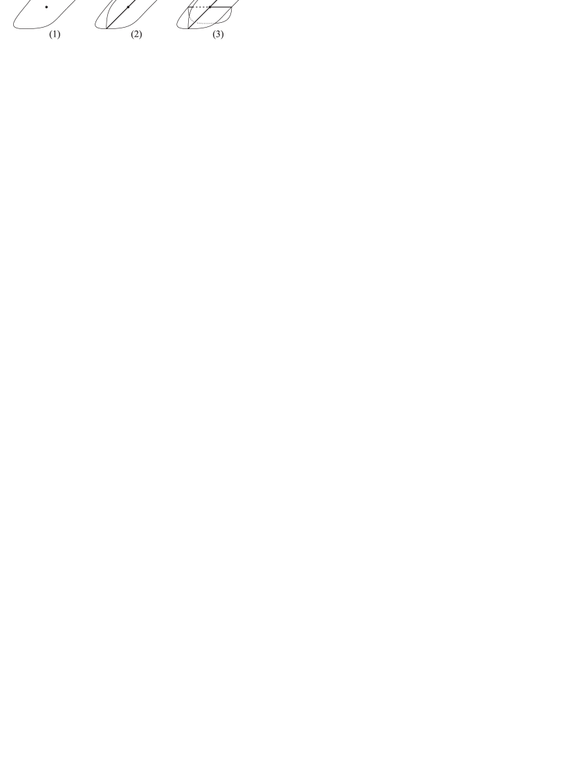
Figure 1: Neighborhoods of points in a standard polyhedron.

Now a point is a spine of $S^{3}$, the projective plane $\mathbb{RP}^{2}$ is a spine of $\mathbb{RP}^{3}$ and the “triple hat” – a triangle with all edges identified in the same direction – is a simple spine of $L_{3,1}$. Since these spines do not contain vertices, we have $c(S^{3})=c(\mathbb{RP}^{3})=c(L_{3,1})=0$. In general, to calculate the complexity of a manifold we must look for its minimal spines, i.e. the simple spines with the lowest number of vertices. It turns out [7, 6] that if $M$ is $\mathbb{P}^{2}$-irreducible and distinct from $S^{3},\mathbb{RP}^{3},L_{3,1}$ then it has a minimal spine which is standard. A polyhedron is standard when every point has a neighborhood of one of the types (1)-(3) shown in Fig. 1, and the sets of such points induce a cellularization of $P$. That is, defining $S(P)$ as the set of points of type (2) or (3), the components of $P\setminus S(P)$ should be open discs – the faces – and the components of $S(P)\setminus V(P)$ should be open segments – the edges. A standard spine is dual to a 1-vertex triangulation of $M$, and this partially explains why $c(M)$ equals the minimal number of tetrahedra in a triangulation when $M$ is $\mathbb{P}^{2}$-irreducible and distinct from $S^{3},\mathbb{RP}^{3},L_{3,1}$.

Sketch of the proof

A closed non-orientable 3-manifold has a non-trivial first Stiefel-Whitney class $w_{1}\in H^{1}(M;\mathbb{Z}_{2})$. A surface $\Sigma\subset M$ which is Poincaré dual to $w_{1}$ is usually called a Stiefel-Whitney surface [4]. It has odd intersection with a loop $\gamma$ if and only if $\gamma$ is orientation-reversing. It follows that $M\setminus\Sigma$ is connected and orientable, i.e. $M=N\cup\mathcal{R}(\Sigma)$ is obtained by gluing a regular neighborhood $\mathcal{R}(\Sigma)$ of $\Sigma$ to an orientable connected compact $N$ along their boundaries.

We can now list the main steps of the proof. Let $M$ be a non-orientable $\mathbb{P}^{2}$-irreducible closed 3-manifold $M$ with $c(M)\leqslant 6$.

• We prove that, without loss of generality, $\Sigma\subset M$ can be assumed to lie in a minimal skeleton $P$ of $M$ so that $\mathcal{R}(\Sigma)\cap P$ (whence $\mathcal{R}(\Sigma)$) has some definite shape;

• using the shape of $\mathcal{R}(\Sigma)\cap P$ we prove that $N$, with a suitable extra structure (a marking on $\partial N$) has a very low (suitably defined) complexity;

• manifolds with marked boundary of low complexity are classified in [5], so we list the possible shapes for $N$;

• we examine by hand how $\mathcal{R}(\Sigma)$ and $N$ can be glued along $\partial\mathcal{R}(\Sigma)=\partial N$, proving that precisely the four flat non-orientable manifolds and the torus bundle over $S^{1}$ of type Sol with monodromy trace $\tiny{\left(\begin{array}[]{@{}c@{\ }c@{}}1&1\\ 1&0\\ \end{array}\right)}$ can arise;

• we exhibit some spines of manifolds of type $\mathbb{H}^{2}\times S^{1}$, of type Sol, and with non-trivial JSJ decomposition with $7$ vertices.

Our results on $\mathcal{R}(\Sigma)\cap P$ are stated in the rest of this section and proved in Section 4. The theory of complexity for manifolds with marked boundary is reviewed in Section 2, and is used in Section 3 to prove that $N$ has low complexity, and hence a definite shape. The possible gluings of $N$ and $\mathcal{R}(\Sigma)$ are then analysed at the end of Section 3, to conclude the proof.

First part of the proof

Let us start with a general result on Stiefel-Whitney surfaces.

Proposition 1.3.

Let $\Sigma\subset M$ be a Stiefel-Whitney surface of a closed non-orientable $M$. The surfaces $\Sigma$ and $\partial\mathcal{R}(\Sigma)$ are orientable. If $M$ is $\mathbb{P}^{2}$-irreducible then:

• $N={\rm Cl}(M\setminus\mathcal{R}(\Sigma))$ is $\mathbb{P}^{2}$-irreducible;

• no component of $\Sigma$ or $\partial\mathcal{R}(\Sigma)$ is a sphere;

• if a component of $\Sigma$ or $\partial\mathcal{R}(\Sigma)$ is a torus then it is incompressible.

Proof.

We first prove that $\Sigma$ is orientable. Suppose $\gamma\subset\Sigma$ is an orientation-reversing loop (in $\Sigma$). If $\gamma$ is orientation-preserving in $M$ it can be perturbed to a loop intersecting $\Sigma$ in one point, and if it is orientation-reversing in $M$ it can be isotoped away from $\Sigma$: both cases being in contrast to the definition of $\Sigma$. Obviously, $\partial\mathcal{R}(\Sigma)$ is orientable because $N$ is.

Suppose now $M$ is $\mathbb{P}^{2}$-irreducible. Since $N$ is connected, each component of $\Sigma$ is non-separating, thus it cannot be a sphere or a compressible torus. So no component of $\partial\mathcal{R}(\Sigma)$ is a sphere. Suppose a component of $\partial\mathcal{R}(\Sigma)$ is a compressible torus. Then the corresponding component of $\mathcal{R}(\Sigma)$ is the non-orientable interval bundle $T\begin{picture}(12.0,12.0)\put(2.0,0.0){$\times$}\put(2.0,4.5){$\sim$}\end{picture}I$ over the torus. It follows quite easily that $M$ is a Dehn filling on $T\begin{picture}(12.0,12.0)\put(2.0,0.0){$\times$}\put(2.0,4.5){$\sim$}\end{picture}I$, hence $S^{2}\begin{picture}(12.0,12.0)\put(2.0,0.0){$\times$}\put(2.0,4.5){$\sim$}\end{picture}S^{1}$ or $\mathbb{P}^{2}\times S^{1}$, a contradiction.

Let $S\subset N$ be a sphere. Then $S$ bounds in $M$ a ball, which cannot contain components of $\Sigma$ because they are non-separating. Hence the ball is contained in $N$, and the orientable $N$ is $\mathbb{P}^{2}$-irreducible. ∎

Let $P$ be a standard spine of a non-orientable $M$. The embedding $P\subset M$ induces an isomorphism $H_{2}(P;\mathbb{Z}_{2})\cong H_{2}(M;\mathbb{Z}_{2})$. Using cellular homology, a representative for a cycle in $H_{2}(P;\mathbb{Z}_{2})$ is a subpolyhedron consisting of some faces, an even number of them incident to each edge of $P$. Such a subpolyhedron is a surface near the edges it contains, and it is also a surface near the vertices (in fact, the link of a vertex does not contain two disjoint circles). Thus every homology class is represented by a (unique) surface in $P$: in particular there is a unique Stiefel-Whitney surface $\Sigma$ inside $P$.

Let us now suppose $M$ is $\mathbb{P}^{2}$-irreducible with $c(M)\leqslant 6$, and $P$ is a minimal standard spine of $M$. The Stiefel-Whitney surface $\Sigma\subset P$ is not necessarily connected but, since $P$ has at most 6 vertices, it contains a few components of low genus. Namely, we have the following result which will be proved in Section 4.

Lemma 1.4.

Let $M$ be $\mathbb{P}^{2}$-irreducible with $c(M)\leqslant 6$ and $P$ be a minimal standard spine of $M$. The Stiefel-Whitney surface $\Sigma\subset P$ contains at most $2$ connected components. Moreover $M$ has a minimal standard spine (which we denote again by $P$) with a Stiefel-Whitney surface (which we denote again by $\Sigma$) having Euler characteristic equal to zero.

So $\Sigma$ consists of one or two tori. We fix a sufficiently small regular neighborhood $\mathcal{R}(\Sigma)$ of $\Sigma$ in $M$, such that the intersection of $\mathcal{R}(\Sigma)$ and $P$ is a regular neighborhood $\mathcal{R}_{P}(\Sigma)$ of $\Sigma$ in $P$. Using the fact that $P$ has 6 vertices at most, we will prove in Section 4 the following results. Recall that there are two interval bundles on the torus up to homeomorphism, namely $T\times I$ and $T\begin{picture}(12.0,12.0)\put(2.0,0.0){$\times$}\put(2.0,4.5){$\sim$}\end{picture}I$.

Lemma 1.5.

Let $M$ be $\mathbb{P}^{2}$-irreducible with $c(M)\leqslant 6$ and $P$ be a minimal standard spine of $M$. If $\Sigma\subset P$ consists of two tori, $\mathcal{R}(\Sigma)$ consists of two copies of $T\begin{picture}(12.0,12.0)\put(2.0,0.0){$\times$}\put(2.0,4.5){$\sim$}\end{picture}I$ and each of the components of $\mathcal{R}_{P}(\Sigma)$ is as shown in Fig. 2.

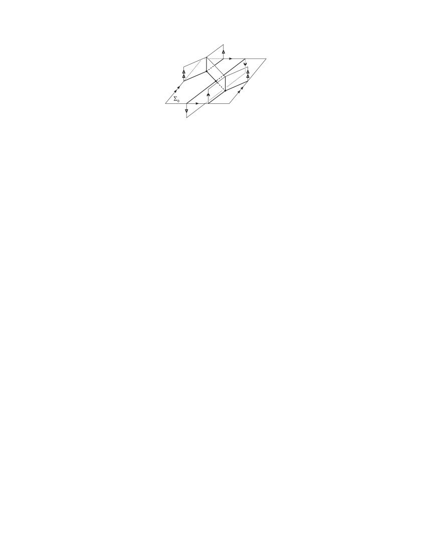
Figure 2: The regular neighborhood (in $P$) of a component $\Sigma_{0}$ of $\Sigma$, such that $\mathcal{R}(\Sigma_{0})=T\widetilde{\times}I$ (similar arrows must be identified).

Lemma 1.6.

Let $M$ be $\mathbb{P}^{2}$-irreducible with $c(M)\leqslant 6$ and $P$ be a minimal standard spine of $M$. If $\Sigma\subset P$ is one torus and $\mathcal{R}(\Sigma)=T\times I$, then $\mathcal{R}_{P}(\Sigma)$ is one of the two polyhedra shown in Fig. 3.

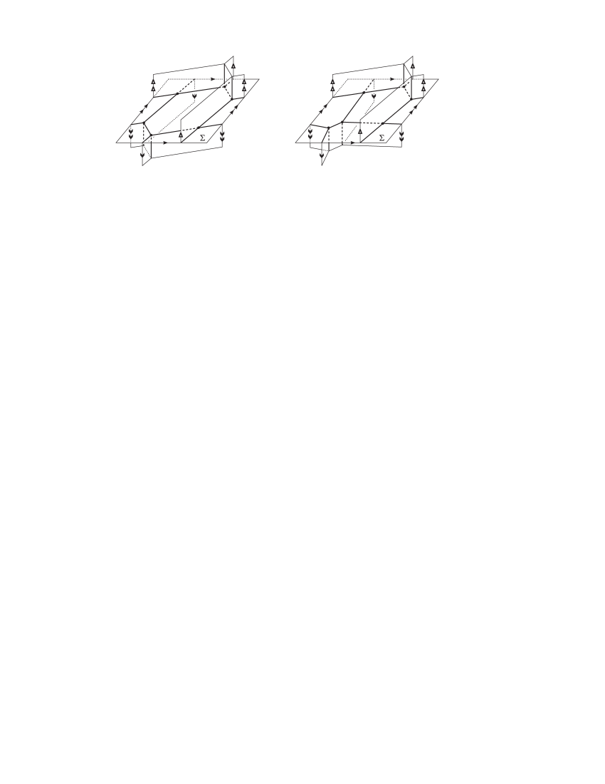
Figure 3: Two possibilities for the regular neighborhood (in $P$) of $\Sigma$, if $\Sigma$ consists of one torus and $\mathcal{R}(\Sigma)=T\times I$ (similar arrows must be identified).

Lemma 1.7.

Let $M$ be $\mathbb{P}^{2}$-irreducible with $c(M)\leqslant 6$ and $P$ be a minimal standard spine of $M$. If $\Sigma\subset P$ is one torus and $\mathcal{R}(\Sigma)=T\begin{picture}(12.0,12.0)\put(2.0,0.0){$\times$}\put(2.0,4.5){$\sim$}\end{picture}I$, then $M$ has a minimal standard spine (which we denote again by $P$) with a Stiefel-Whitney surface $\Sigma$ such that $\mathcal{R}(\Sigma)=T\begin{picture}(12.0,12.0)\put(2.0,0.0){$\times$}\put(2.0,4.5){$\sim$}\end{picture}I$ and $\mathcal{R}_{P}(\Sigma)$ is as shown in Fig. 2.

We now know that $\mathcal{R}_{P}(\Sigma)$ has 3 possible shapes. In order to complete our classification, we need to know the possible shapes of the rest of $P$, namely the polyhedron $Q={\rm Cl}(P\setminus\mathcal{R}_{P}(\Sigma))$. Moreover, we know that the two polyhedra are glued along a very special graph contained in $\partial\mathcal{R}(\Sigma)$: it consists of either one or two $\theta$-graphs. Here, a $\theta$-graph is a trivalent graph $\theta$ contained in a torus $T$ such that $T\setminus\theta$ is an open disc. Decompositions of minimal spines (and manifolds) along $\theta$-graphs (and tori) have been studied in [5, 6]. The basic result is a decomposition theorem for $\mathbb{P}^{2}$-irreducible manifolds. Since we will use it on $N$, which is orientable, we describe in Section 2 the orientable version of the theory. (We only note here that non-orientable manifolds could be cut along Klein bottles also, and the graph should be taken into account in this case.) We will then conclude the proof of Theorem 1.2 in Section 3.

2 Manifolds with marked boundary

$\theta$-graphs in the torus

A $\theta$-graph in the torus $T$ is a trivalent graph $\theta\subset T$ such that $T\setminus\theta$ is an open disc. The embedding of $\theta$ in $T$ is unique up to homeomorphism of $T$, but not up to isotopy. There is a nice description, taken from [2], of all $\theta$-graphs (up to isotopy) which we now describe. After fixing a basis $(a,b)$ for $H_{1}(T;\mathbb{Z})$, every slope on $T$ (i.e. isotopy class of simple closed essential curves) is determined by its unsigned homology class $\pm(pa+qb)$, thus by the number $p/q\in\mathbb{Q}\cup\{\infty\}$. Consider $\mathbb{Q}\cup\{\infty\}$ sitting inside $\mathbb{R}\cup\{\infty\}$, the boundary of the upper half-plane of $\mathbb{C}$, with its standard hyperbolic metric. For each pair $p/q,r/s$ of slopes having algebraic intersection $\pm 1$ (i.e. such that $ps-qr=\pm 1$) draw a geodesic connecting $p/q$ and $r/s$. The result is a tesselation of the half-plane into ideal triangles, shown in Fig. 4-left (in the disc model).

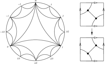
Figure 4: A tesselation of the Poincaré disc into ideal triangles (left) and a flip (right).

It is easily seen that a $\theta$-graph is determined by the three slopes it contains, and that such slopes have pairwise intersection 1. Thus, a $\theta$-curve corresponds to a triangle of the ideal tesselation, i.e. to a vertex of the dual trivalent tree. Moreover, two $\theta$-graphs are connected by a segment in this tree when they share two slopes, i.e. when we can pass from one $\theta$-graph to the other via a flip, shown in Fig. 4-right.

Manifolds with marked boundary

Let $M$ be a connected compact 3-manifold with (possibly empty) boundary consisting of tori. By associating to each torus component of $\partial M$ a $\theta$-graph, we get a manifold with marked boundary. As we have seen, the same manifold can be marked in infinitely many distinct ways.

Now we describe two fundamental operations on the set of manifolds with marked boundary. The first one is binary: if $M$ and $M^{\prime}$ are two such objects, take two tori $T\subset\partial M,T^{\prime}\subset\partial M^{\prime}$ marked with $\theta\subset T,\theta^{\prime}\subset T^{\prime}$ and a homeomorphism $\psi:T\stackrel{{\scriptstyle\sim}}{{\rightarrow}}T^{\prime}$ such that $\psi(\theta)=\theta^{\prime}$. By gluing $M$ and $M^{\prime}$ along $\psi$ we get a new 3-manifold with marked boundary. We call this operation an assembling. Note that, although there are infinitely many non-isotopic maps between two tori, only finitely many of them send one marking to the other, so there is a finite number of non-equivalent assemblings of $M$ and $M^{\prime}$.

We describe the second operation. Let $M$ be a manifold with marked boundary, and $T,T^{\prime}$ be two distinct boundary components of it, marked with $\theta\subset T$ and $\theta^{\prime}\subset T^{\prime}$. Let $\psi:T\stackrel{{\scriptstyle\sim}}{{\rightarrow}}T^{\prime}$ be a homeomorphism such that $\psi(\theta)$ equals either $\theta^{\prime}$ or a $\theta$-graph obtained from $\theta^{\prime}$ via a flip. The manifold obtained identifying $T$ and $T^{\prime}$ via $\psi$ is a new manifold with marked boundary. (There is a technical reason for not asking only that $\psi(\theta)=\theta^{\prime}$, which will be clear later.) We call this operation a self-assembling. Again, there is only a finite number of non-equivalent self-assemblings.

Spines and skeleta

The notion of spine extends to the class of manifolds with marked boundary. A sub-polyhedron $P$ of a 3-manifold with marked boundary $M$ is called a skeleton of $M$ if $M\setminus(P\cup\partial M)$ is an open ball and $P\cap\partial M$ is a graph contained in the marking of $\partial M$. We have not used the word “spine” because maybe $P$ is not a spine of $M$ in the usual sense when $\partial M\neq\emptyset$ – i.e. $M$ does not retract onto $P$. On the other side note that, if $M$ is closed, a skeleton of $M$ is just a spine of $M$. Recall that a polyhedron is simple when the link of every point is contained in the 1-skeleton of a tetrahedron $K$. It is easy to prove that each 3-manifold with marked boundary has a simple skeleton.

Complexity

The complexity of a 3-manifold with marked boundary $M$ is of course defined as the minimal number of vertices of a simple skeleton of $M$. It depends on the topology of $M$ and on the marking. In particular, if $T=\partial M$ is one torus then every (isotopy class of a) $\theta$-graph on $T$ gives a distinct complexity for $M$. Three properties extend from the closed case to the case with marked boundary: complexity is still additive under connected sums, it is finite-to-one on orientable irreducible manifolds with marked boundary, and if $M$ is orientable irreducible with $c(M)>0$, then it has a minimal standard skeleton [5]. A skeleton $P\subset M$ is called standard when $P\cup\partial M$ is.

Examples

Let $T$ be the torus. Consider $M=T\times I$, the boundary being marked with a $\theta_{0}\subset T\times 0$ and a $\theta_{1}\subset T\times 1$. If $\theta_{0}$ and $\theta_{1}$ are isotopic, the resulting manifold with marked boundary is called $B_{0}$. If $\theta_{0}$ and $\theta_{1}$ are related by a flip, we call the resulting manifold with marked boundary $B_{3}$. A skeleton for $B_{0}$ is $\theta_{0}\times[0,1]$, while a skeleton for $B_{3}$ is shown in Fig. 5. The skeleton of $B_{0}$ has no vertices, so $c(B_{0})=0$. The skeleton of $B_{3}$ has 1 vertex, and it can be shown [5] that there is no skeleton for $B_{3}$ without vertices, so $c(B_{3})=1$.

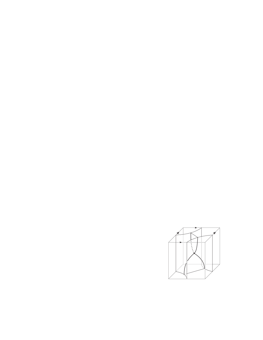
Figure 5: A skeleton for $B_{3}$.

Two distinct marked solid tori are shown in Fig. 6 (left and centre) and denoted by $B_{1}$ and $B_{2}$. A skeleton for $B_{1}$ is a meridinal disc with boundary contained in the $\theta$-graph. A skeleton for $B_{2}$ is shown in Fig. 6-right. Since they have no vertices, we have $c(B_{1})=c(B_{2})=0$.

The first irreducible orientable manifold with more than two marked boundary components has $c=3$. Let $D_{2}$ be a disc with two holes. Set $M=D_{2}\times S^{1}$. For each torus $T$ in $\partial M$, a basis $(a,b)$ for $H_{1}(T;\mathbb{Z})$ is given by taking $a$ to be $\partial D_{2}\times\{{\rm pt}\}$ (with orientation induced from that of $D_{2}$) and $b$ to be $\{{\rm pt}\}\times S^{1}$, oriented as $S^{1}$. With respect to this basis, on each boundary component a triple of slopes $\{i,\infty,i+1\}$ defines a $\theta$-graph $\theta_{i}$ for any integer $i$ (note that $\theta_{-1}$ and $\theta_{0}$ are the $\theta$-graphs containing $0$ and $\infty$). Now let $B_{4}$ be $M$ with markings $\theta_{0},\theta_{0}$ and $\theta_{-1}$, see Fig. 7-left. It has a skeleton with 3 vertices, shown in Fig. 7-right. It can be proved [5] that $B_{4}$ has no skeleton with less vertices, so $c(B_{4})=3$, and that a distinct choice for the markings – for instance the same $\theta_{0}$ on all boundary components – would give $c>3$.

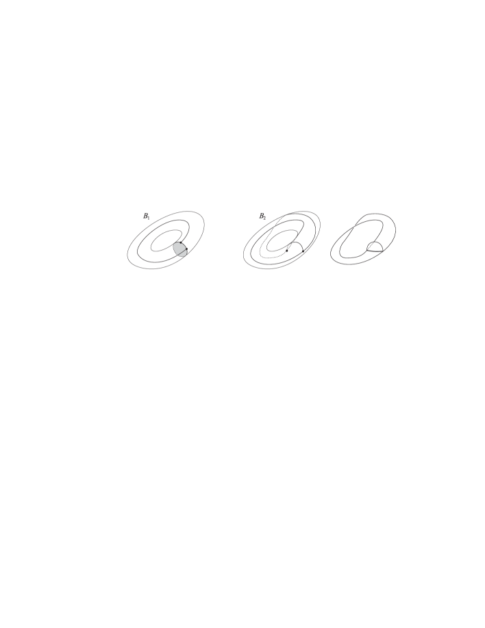
Figure 6: The manifolds with marked boundary $B_{1}$ (left) and $B_{2}$ (centre), and a skeleton for $B_{2}$ (right).

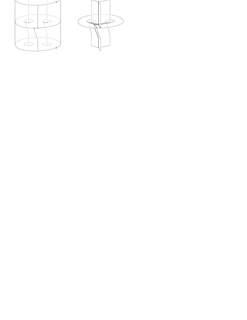
Figure 7: The manifold with marked boundary $B_{4}$ (left) and a skeleton for it (right).

Assemblings and skeleta

Let $M,M^{\prime}$ be two manifolds with marked boundary, and $P,P^{\prime}$ be two corresponding standard skeleta. An assembling of $M$ and $M^{\prime}$ is given by a map $\psi$ that matches the $\theta$-graphs, so $P\cup_{\psi}P^{\prime}$ is a simple polyhedron inside $M\cup_{\psi}M^{\prime}$. Moreover, it is not difficult to see that $P\cup_{\psi}P^{\prime}$ is a skeleton of the new manifold with marked boundary $M\cup_{\psi}M^{\prime}$. (This is true because the complement of a $\theta$-graph is a single disc, so the complement of $P\cup_{\psi}P^{\prime}$ consists of two balls glued together along a single disc, hence another ball.)

If $P,P^{\prime}$ have $n,n^{\prime}$ vertices, then $P\cup_{\psi}P^{\prime}$ has $n+n^{\prime}$ vertices. Suppose $P$ and $P^{\prime}$ are minimal skeleta of $M$ and $M^{\prime}$, i.e. $n$ and $n^{\prime}$ are the complexities of $M$ and $M^{\prime}$. It is not true in general that $P\cup_{\psi}P^{\prime}$ is minimal. Since $M\cup_{\psi}M^{\prime}$ has a skeleton with $n+n^{\prime}$ vertices, its complexity is at most $n+n^{\prime}$, and it equals $n+n^{\prime}$ precisely when $P\cup_{\psi}P^{\prime}$ is minimal. We will be interested in the case when $P\cup_{\psi}P^{\prime}$ is minimal: in other words, complexity is sub-additive under assemblings, and we will be interested in the case when it is additive.

An analogous construction works for self-assemblings. Let $M^{\prime}$ be obtained self-assembling $M$, along a map $\psi:T\stackrel{{\scriptstyle\sim}}{{\to}}T^{\prime}$ such that $\psi(\theta)$ either equals $\theta^{\prime}$ or is obtained from $\theta^{\prime}$ via a flip. In any case, it is possible to isotope $\psi$ to $\psi^{\prime}$ so that $\psi^{\prime}(\theta)$ and $\theta^{\prime}$ intersect each other transversely in 2 points, and to use the map $\psi^{\prime}$ to construct $M^{\prime}$. Let $P$ be a standard skeleton for $M$. Take $P^{\prime}=P\cup T$ inside $M^{\prime}$: again, $P^{\prime}$ is a skeleton for $M^{\prime}$. The polyhedron $P^{\prime}$ is the result of adding one of the two polyhedra shown in Fig. 3 to $P$. (Note that a construction analogous to the one made for assemblings does not work: if $\psi(\theta)=\theta^{\prime}$, then $P$ alone inside $M^{\prime}$ is not a skeleton of $M^{\prime}$, because its complement is a solid torus: this is why it is necessary to add $T$. Moreover $P\cup T$ is a skeleton but is not standard, so we need to isotope $\psi$ to recover standardness.) This operation creates 6 new vertices: if $P$ has $n$ vertices, then $P^{\prime}$ has $n+6$ vertices. So the complexity of $M^{\prime}$ is at most the complexity of $M$ plus 6.

Bricks

The theory ends with a decomposition theorem. An assembling is sharp if the complexity is additive and both manifolds with marked boundary are irreducible and distinct from $B_{0}$, and a self-assembling is sharp if the complexity of the new manifold is the complexity of the old one plus 6. An irreducible orientable manifold with marked boundary is a brick if it is not the result of a sharp assembling or self-assembling of other irreducible manifolds with marked boundary. The proof of the following result is clear: if an irreducible manifold with marked boundary is not a brick, then it can be de-assembled. Then we repeat the analysis on each new piece. Since the sum of the complexities of all pieces does not increase (and since the only possible pieces with complexity 0 are known to be $B_{1}$ and $B_{2}$), this iteration must stop after finite time.

Proposition 2.1.

Every irreducible orientable manifold with marked boundary can be obtained from some bricks via a combination of sharp assemblings and sharp self-assemblings.

This result can be restated at the level of skeleta: every orientable manifold with marked boundary has a minimal skeleton which splits along $\theta$-graphs into minimal skeleta of bricks. Here, bricks are defined to be orientable. (Non-orientable bricks are analogously defined in [6], but we do not need them here.)

It is proved in [5] that the only bricks with boundary having complexity at most 3 are the $B_{0},\ldots,B_{4}$ introduced above. Using a computer, all bricks $B_{0},\ldots,B_{10}$ having complexity up to 9 and with non-empty boundary have been classified. Let $P_{i}$ be a minimal skeleton of $B_{i}$: Proposition 2.1 implies that every orientable manifold having complexity at most $9$ has a minimal spine which splits along $\theta$-graphs into copies of $P_{1},\ldots,P_{10}$. Bricks $B_{5},\ldots,B_{10}$ have complexity $8$ or $9$, moreover they are all hyperbolic except $B_{5}$.

Assembling small bricks

Let $M$ be a manifold with marked boundary. Let us examine the effect of assembling $M$ with some $B_{i}$ along a torus $T\subset\partial M$, marked with a $\theta\subset T$. Choose a basis for $H_{1}(T;\mathbb{Z})$ so that $\theta$ corresponds to the triple $\{0,1,\infty\}$, see Fig. 4-left. If $i=0$, the assembling leaves $M$ unaffected. If $i=1$, a Dehn filling is performed on $M$, killing one of the three slopes $0,1,\infty$. If $i=2$, a Dehn filling is performed on $M$, killing one of the slopes $2,1/2,-1$. If $i=3$, the graph $\theta$ is changed by a flip. It follows that by assembling $M$ with some copies of $B_{1},B_{2},$ and $B_{3}$ we can arbitrarily change some markings or do arbitrary Dehn fillings on $M$.

We can use Proposition 2.1 and the known list of bricks to classify manifolds with non-empty marked boundary of low complexity. Every such manifold is obtained via sharp assemblings and self-assemblings from the known bricks. For instance, if a marked $M$ has complexity at most 2, no self-assembling is involved since it adds 6 to the complexity, and only assemblings of $B_{0},B_{1},B_{2},$ and $B_{3}$ are involved. Therefore $M$ is a (marked) solid torus, or a (marked) product $T\times I$. We are here interested in the first case where $M$ has one boundary component and is not a (marked) solid torus. Let $(D_{2}\times S^{1})_{2,2,\theta_{-1}}$ be the Seifert manifold with base space a disc and two fibers of type $(2,1)$, marked with $\theta_{-1}$ in the boundary. (Recall that $\theta_{-1}$ is the $\theta$-graph containing the slopes $\infty,-1,$ and $0$, where coordinates are taken with respect to the obvious basis of $H_{1}(D_{2}\times S^{1};\mathbb{Z})$.)

Proposition 2.2.

Every irreducible manifold with a single marked boundary component having $c\leqslant 2$ is a marked solid torus. Every such manifold having $c=3$ is a marked solid torus or $(D_{2}\times S^{1})_{2,2,\theta_{-1}}$.

Proof.

Suppose $M$ is not a marked solid torus, with $c\leqslant 3$. It decomposes into copies of $B_{1},B_{2},B_{3},$ and $B_{4}$, and at least one $B_{4}$ must be present. Moreover, since $c(B_{4})=3$, the other bricks in the assembling have complexity 0, so they must be $B_{1}$’s and $B_{2}$’s. Despite the apparent lack of symmetry of the markings, for each pair of boundary components there is an automorphism of $B_{4}$ interchanging them (and their markings), so it is not important to which boundary components the $B_{1}$’s and $B_{2}$’s are assembled. Suppose then the assemblings are performed on the first two components. It follows from the discussion above that we can realize Dehn fillings on slopes $\infty,0,1$ with $B_{1}$ and on slopes $-1,1/2,2$ with $B_{2}$. The only such filling that creates a singular fiber is $2$, whence the result. ∎

A manifold with non-trivial JSJ decomposition containing hyperbolic pieces

It is now easy to use the known bricks to build manifolds. Using $B_{1},B_{2},B_{3},$ and $B_{4}$ any graph manifold can be built. The brick $B_{6}$ is the first hyperbolic brick, having $c=8$ (whereas $B_{7},\ldots,B_{10}$ have $c=9$, see [5]). It is the figure-eight knot sister, denoted by $M2^{1}_{2}$ in [1], marked with the most natural $\theta$-graph: it is the $\theta$-graph containing the 3 shortest slopes in the cusp, or equivalently the unique $\theta$-graph fixed by any isometry of $M2^{1}_{2}$. Note that any other marked hyperbolic manifold has $c>8$: the manifold $M2^{1}_{2}$ is then in some sense ‘smaller’ (or ‘simpler’) than the figure-8 knot complement $M2^{1}_{1}$, although they have the same volume – note that the smallest known closed hyperbolic manifold is obtained via Dehn filling from $M2^{1}_{2}$ but not from $M2^{1}_{1}$.

If we assemble $B_{6}$ with $B_{1}$ or $B_{2}$, we always get a non-hyperbolic manifold: in order to get a hyperbolic one, we must use a $B_{3}$ and a $B_{2}$, which is coherent with the fact that the first closed hyperbolic manifolds have $c=9=8+1=c(B_{6})+c(B_{3})$. It is easier to construct a closed manifold whose JSJ decomposition is non-trivial and contains a hyperbolic piece: simply take any assembling of $B_{6}$ and $(D_{2}\times S^{1})_{2,2,\theta_{-1}}$. The complexities of the pieces are $8$ and $3$, so we get a manifold with $c\leqslant 11$, but we cannot be sure that equality holds – in other words, by gluing minimal spines of $B_{6}$ and $(D_{2}\times S^{1})_{2,2,\theta_{-1}}$ we get a spine of the closed manifold, which is possibly not minimal. Nevertheless, we know from [5] that every brick with $c\leqslant 9$ is atoroidal. If this were true for any $c$, every sharp decomposition of a closed irreducible manifold into bricks would be a refinement of its JSJ decomposition. In other words, there would be a minimal spine of the closed manifold which decomposes into minimal skeleta of the pieces of the JSJ decomposition (which might further decompose), with appropriate markings. Therefore, the complexity of a closed manifold would be the sum of the complexities of the (appropriately marked) pieces of its JSJ decomposition: in particular, a hyperbolic piece would give a contribution $\geqslant 8$, and a Seifert one a contribution $\geqslant 3$, giving $8+3=11$ at least.

3 End of the proof

At the end of Section 1, we have listed the possible shapes for the regular neighborhood $\mathcal{R}_{P}(\Sigma)$ of the Stiefel-Whitney surface $\Sigma$ in $P$. In all cases, the polyhedron $P$ can be cut into a (possibly disconnected) $\mathcal{R}_{P}(\Sigma)$ and a connected $Q={\rm Cl}(P\setminus\mathcal{R}_{P}(\Sigma))$. The two subpolyhedra are glued along $\theta$-graphs. At the level of manifolds, $\mathcal{R}_{P}(\Sigma)$ is contained in $\mathcal{R}(\Sigma)$ and $Q$ is contained in $N$, which is orientable and irreducible. The original $\mathbb{P}^{2}$-irreducible $M$ is decomposed along one or two tori into $\mathcal{R}(\Sigma)$ and $N$. Both $\mathcal{R}(\Sigma)$ and $N$ are equipped with a marking on each boundary component, given by the $\theta$-graphs separating the polyhedra. It is easy to check that $N\setminus(\partial N\cup Q)$ is an open ball in any case, so $Q$ is a skeleton of $N$. Concerning the 3 possible shapes for $\mathcal{R}_{P}(\Sigma)$, two of them are skeleta of the corresponding $\mathcal{R}(\Sigma)$, and the other one is not. We now study this in detail.

If $\Sigma$ consists of two tori

Each component of $\mathcal{R}_{P}(\Sigma)$ is a skeleton (with 3 vertices) of the corresponding marked $T\begin{picture}(12.0,12.0)\put(2.0,0.0){$\times$}\put(2.0,4.5){$\sim$}\end{picture}I$. Therefore $M$ is obtained assembling a copy of the marked $T\begin{picture}(12.0,12.0)\put(2.0,0.0){$\times$}\put(2.0,4.5){$\sim$}\end{picture}I$ on each boundary component of $N$. Since $\mathcal{R}_{P}(\Sigma)$ has 6 vertices and $P$ has $6$ vertices at most, there is no vertex in $Q$, so $N$ has complexity zero (and it is orientable), hence $N=B_{0}$ is the trivial brick. Thus $M$ is obtained assembling two copies of the marked $T\begin{picture}(12.0,12.0)\put(2.0,0.0){$\times$}\put(2.0,4.5){$\sim$}\end{picture}I$.

We now prove that the result of this assembling must be a flat manifold. Note that $T\begin{picture}(12.0,12.0)\put(2.0,0.0){$\times$}\put(2.0,4.5){$\sim$}\end{picture}I$ has two distinct fibrations: the first one is the product $S\times S^{1}$, where $S$ is the Möbius strip. The second one is a Seifert fibration over the orbifold whose underlying topological space is an annulus, with one mirror circle (so the orbifold has only one true boundary component, see [9]). A basis $(a,b)$ for $H_{1}(\partial(S\times S^{1});\mathbb{Z})$ is given by taking $a=\partial S\times\{{\rm pt}\}$ and $b=\{{\rm pt}\}\times S^{1}$, with some orientations. With respect to this basis, slopes are numbers in $\mathbb{Q}\cup\{\infty\}$, and $0$ is a fiber of the first fibration, while $\infty$ is a fiber of the second fibration. The $\theta$-graph in the boundary is the one containing the slopes $\infty,0,1$. An assembling of two copies of $S\times S^{1}$ is given by a map $\psi$ which matches the markings, i.e. sends the set of slopes $\{\infty,0,1\}$ of the first one to the set $\{\infty,0,1\}$ of the other one.

If $\psi(0)=0$, we get a fibration over the Klein bottle. If $\psi(0)=\infty$ or $\psi(\infty)=0$, we get a fibration over a Möbius strip with one mirror circle. If $\psi(\infty)=\infty$, we get a fibration over an annulus with two mirror circles. In all cases the base orbifold has $\chi^{\rm orb}=0$, so the manifold is flat.

If $\Sigma$ is one torus and $\mathcal{R}(\Sigma)=T\widetilde{\times}I$

The polyhedron $\mathcal{R}_{P}(\Sigma)$ is a skeleton of the marked $T\begin{picture}(12.0,12.0)\put(2.0,0.0){$\times$}\put(2.0,4.5){$\sim$}\end{picture}I$. Therefore $M$ is obtained by assembling $N$ with $T\begin{picture}(12.0,12.0)\put(2.0,0.0){$\times$}\put(2.0,4.5){$\sim$}\end{picture}I$. Since $\mathcal{R}_{P}(\Sigma)$ has 3 vertices, there are three vertices at most in $Q$. Proposition 1.3 implies that $N$ is not a (marked) solid torus, hence $N=(D_{2}\times S^{1})_{2,2,\theta_{-1}}$ by Proposition 2.2.

As above, we prove that the result of this assembling must be a flat manifold. Note first that $(D_{2}\times S^{1})_{2,2,\theta_{-1}}$ fibers over a disc with two singular fibers of type $(2,1)$, or as a twisted product $S\begin{picture}(12.0,12.0)\put(2.0,0.0){$\times$}\put(2.0,4.5){$\sim$}\end{picture}S^{1}$ over the Möbius strip $S$. The $\theta$-curve $\theta_{-1}$ contains the slopes $\infty,-1,0$, and $0$ is a fiber of the first fibration, while $-1$ is a fiber of the second fibration. Now, an assembling is given by a map $\psi$ that sends the triple of slopes $\{\infty,-1,0\}$ of $N$ to the triple of slopes $\{\infty,0,1\}$ of $T\begin{picture}(12.0,12.0)\put(2.0,0.0){$\times$}\put(2.0,4.5){$\sim$}\end{picture}I$. If $\psi(0)=0$, we get a fibration over $\mathbb{RP}^{2}$ with two singular fibers of type $(2,1)$. If $\psi(0)=1$ we get a fibration over a disc with two singular fibers of type $(2,1)$ and a mirror circle. If $\psi(-1)=0$ we get a fibration over a Klein bottle, and if $\psi(-1)=1$ we get a fibration over a Möbius strip with one mirror circle. In all cases the base orbifold has $\chi^{\rm orb}=0$, so the manifold is flat.

If $\Sigma$ is one torus and $\mathcal{R}(\Sigma)=T\times I$

The polyhedron $\mathcal{R}_{P}(\Sigma)$ is not a skeleton of the marked $T\times I$, since $(T\times I)\setminus(\partial(T\times I)\cup\mathcal{R}_{P}(\Sigma))$ consists of two balls instead of one. The polyhedron $\mathcal{R}_{P}(\Sigma)$ is one involved in self-assemblings, so our $M$ is the result of a self-assembling of $N$, which has two boundary components and complexity 0 (because 6 vertices are in $\mathcal{R}_{P}(\Sigma)$). Therefore $M$ is a self-assembling of $B_{0}$, i.e. it is the mapping torus of a map $\psi:T\to T$ that sends a $\theta$-graph $\theta\subset T$ to a $\theta$-graph $\psi(\theta)$ sharing at least two slopes with $\theta$. Let $a,b\in H_{1}(T;\mathbb{Z})$ represent these two slopes. With respect to the basis $(a,b)$, we have $\psi(0),\psi(\infty)\in\{0,1,\infty\}$, therefore $\psi$ is read as a matrix $A$, with trace between $-1$ and $1$ (recall that $M$ is non-orientable), which is either periodic or hyperbolic. In the former case $M$ is flat, while in the latter one $M$ is a torus bundle (of type Sol) with monodromy $A$ (see [9]). Obviously, these self-assemblings are sharp because $P$ is minimal. Now, it is easy to prove that every non-periodic matrix $A\in{\rm GL}_{2}(\mathbb{Z})$ with $\det A=-1$ and $|{\rm tr}\,A|\leqslant 1$ is conjugated either to $\tiny{\left(\begin{array}[]{@{}c@{\ }c@{}}1&1\\ 1&0\\ \end{array}\right)}$ or to $\tiny{\left(\begin{array}[]{@{}c@{\ }c@{}}1&1\\ 1&0\\ \end{array}\right)}^{{\tiny-1}}=\tiny{\left(\begin{array}[]{@{}c@{\ }c@{}}0&1\\ 1&-1\\ \end{array}\right)}$ (so ${\rm tr}\,A=\pm 1$), hence there is only one such manifold of type Sol.

Conclusion

We have proved that every closed non-orientable $\mathbb{P}^{2}$-irreducible manifold with $c\leqslant 6$ either is flat or it is the torus bundle (of type Sol) with monodromy $\tiny{\left(\begin{array}[]{@{}c@{\ }c@{}}1&1\\ 1&0\\ \end{array}\right)}$, and that it has complexity 6. Moreover, each of these 5 manifolds occurs. In fact, each of the 4 flat manifolds fibres in a few distinct ways over 1- or 2-dimensional orbifolds, and it follows from [9] that all 4 can be realized with some of the fibrations described above. Moreover, the Sol manifold has been constructed by self-assembling $B_{0}$ sharply.

Examples of non-orientable manifolds with complexity 7

Using $T\begin{picture}(12.0,12.0)\put(2.0,0.0){$\times$}\put(2.0,4.5){$\sim$}\end{picture}I$, $B_{4}$, $B_{3}$, and two $B_{2}$’s, it is now easy to construct closed manifolds of complexity $7$. We have seen that a Dehn filling killing a slope in $\{\infty,0,1,-1,1/2,2\}$ on the first component of $\partial B_{4}$ can be realized assembling $B_{1}$ or $B_{2}$. We can kill the slope $3$ as follows: we first assemble $B_{3}$, so that $\theta_{0}$ is replaced by $\theta_{1}$ (the $\theta$-graph corresponding to $\{1,2,\infty\}$), and then we assemble $B_{2}$. Therefore the manifold with marked boundary $(D_{2}\times S^{1})_{3,2,\theta_{-1}}$, obtained from $B_{4}$ by filling the first two boundary components along the slopes $3$ and $2$, can be realized with a $B_{4}$, a $B_{3}$, and two $B_{2}$’s, thus it has complexity at most $4$. Now we can assemble it with the marked $T\begin{picture}(12.0,12.0)\put(2.0,0.0){$\times$}\put(2.0,4.5){$\sim$}\end{picture}I$ considered above, along a map $\psi$. The manifold $(D_{2}\times S^{1})_{3,2,\theta_{-1}}$ has one fibration only, with fiber $0$, whereas $T\begin{picture}(12.0,12.0)\put(2.0,0.0){$\times$}\put(2.0,4.5){$\sim$}\end{picture}I$ has two, with fibers $0$ and $\infty$. If $\psi(0)=0$, we get a Seifert fibration over $\mathbb{R}\mathbb{P}^{2}$ with two critical fibres with Seifert invariants $(3,1)$ and $(2,1)$. If $\psi(0)=\infty$, we get a Seifert fibration over the disc with one reflector circle and two critical fibres with Seifert invariants $(3,1)$ and $(2,1)$. In both cases we get $\chi^{\rm orb}<0$, hence a manifold of type $\mathbb{H}^{2}\times\mathbb{R}$. Moreover, the complexity is $4+3=7$ at most, hence it is $7$.

A manifold of type Sol with $c=7$ can be easily constructed as above, with a self-assembling of $B_{3}$ realizing the monodromy $\tiny{\left(\begin{array}[]{@{}c@{\ }c@{}}2&1\\ 1&0\\ \end{array}\right)}$ by sending $\{\infty,0,1\}$ to $\{2,\infty,3\}$.

4 Proofs of the lemmas

We conclude with the proofs of the four lemmas of Section 1. First, we state (and prove) some easy properties of a minimal standard spine of a non-orientable manifold with arbitrary number of vertices. Then, we prove the lemmas.

The following criteria for non-minimality are proved in [5, 6]. Let $P$ be a standard spine of a closed $\mathbb{P}^{2}$-irreducible manifold. Then:

1. If a face of $P$ is embedded and incident to 3 or fewer vertices, $P$ is not minimal.

2. If a loop, embedded in $P$, intersects transversely the singularity of $P$ in 1 point and bounds a disc in the complement of $P$, then $P$ is not minimal.

Throughout this section we suppose $P$ to be a minimal standard spine of a non-orientable manifold $M$. In the first part of this section we do not ask that $c(M)\leqslant 6$, so we allow $P$ to have an arbitrary number of vertices. After, when we will prove the four lemmas, we will come back to the case when $P$ has at most $6$ vertices. As above we call $\Sigma$ the Stiefel-Whitney surface of $M$ contained in $P$. We fix a small regular neighborhood $\mathcal{R}(\Sigma)$ of $\Sigma$ in $M$, such that the intersection of $\mathcal{R}(\Sigma)$ and $P$ is a regular neighborhood of $\Sigma$ in $P$. We denote by $p:\partial\mathcal{R}(\Sigma)\to\Sigma$ the projection. Then $(\mathcal{R}(\Sigma)\setminus\Sigma)\cap P=G\times[0,1)$, where $G=P\cap\partial\mathcal{R}(\Sigma)$ is a trivalent graph. The graph $p(G)$ has vertices with valence 3 and 4, and it is the intersection of $\Sigma$ and the singular set $S(P)$ of $P$. The map $p:G\to\Sigma$ is a transverse immersion, i.e. it is injective except in some pairs of points of $G$, that have the same image, creating the 4-valent vertices of $p(G)$. See an important example in Fig. 8 with $\Sigma$ a torus and $\mathcal{R}(\Sigma)=T\begin{picture}(12.0,12.0)\put(2.0,0.0){$\times$}\put(2.0,4.5){$\sim$}\end{picture}I$. The graphs $G$ and $p(G)$ fulfill some requirements, due to the minimality of $P$.

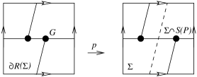
Figure 8: An example of map $p$.

Lemma 4.1.

No component of $G$ is contained in a disc of $\partial\mathcal{R}(\Sigma)$.

Proof.

Suppose a component $G_{0}$ is contained in a disc. If $p$ is injective on $G_{0}$, then $p(G_{0})$ is connected and contained in a disc of $\Sigma$, but $\Sigma\setminus p(G)$ consists of discs (because $P$ is standard), a contradiction. If $p$ is not injective on $G_{0}$, then $p(G)$ intersects some edges of $p(G\setminus G_{0})$. But we can shrink and isotope $G_{0}$, and consequently $G_{0}\times[0,1)$ and $p(G_{0})$, so that $p(G_{0})$ does not intersect any edge of $p(G\setminus G_{0})$. The result is another spine of the same manifold, but with fewer vertices: a contradiction. ∎

Since $P$ is standard, $\Sigma\setminus p(G)$ consists of discs. Concerning $\partial\mathcal{R}(\Sigma)$, we can only prove that $\partial\mathcal{R}(\Sigma)\setminus G$ can be embedded in the 2-sphere and that it consists of discs inside the torus components of $\partial\mathcal{R}(\Sigma)$.

Lemma 4.2.

The set $\partial\mathcal{R}(\Sigma)\setminus G$ can be embedded in the $2$-sphere.

Proof.

The set $\partial\mathcal{R}(\Sigma)\setminus G$ can be seen as a subset of the regular neighborhood $\mathcal{R}(P)$ of $P$ in $M$ which is a sphere (because $M\setminus P$ is a ball). ∎

Lemma 4.3.

Let $T$ be a torus component of $\partial\mathcal{R}(\Sigma)$. Then $T\setminus G$ consists of discs.

Proof.

Suppose a component $C$ of $T\setminus G$ contains a loop $\alpha$ essential in $C$. Then $\alpha$ is essential in the whole of $\partial\mathcal{R}(\Sigma)$ by Lemma 4.1. The loop $\alpha$ is unknotted in the ball $M\setminus P$, thus it bounds a disc. Therefore $T$ is compressible in $N$, in contrast to Proposition 1.3. ∎

Since $\Sigma\setminus p(G)$ consists of discs, connected components of $p(G)$ correspond to connected components of $\Sigma$.

Lemma 4.4.

Every connected component of $p(G)$ contains at least one $4$-valent vertex.

Proof.

Let $\Sigma_{0}$ be a connected component of $\Sigma$. The graph $p(G)\cap\Sigma_{0}$ is a connected component of $p(G)$ and $\Sigma_{0}\setminus(p(G)\cap\Sigma_{0})$ is made of discs. These two facts easily imply that if $p(G)\cap\Sigma_{0}$ contains only 3-valent vertices then $P$ lays on a well-defined side of $\Sigma_{0}$, so we can choose a transverse orientation for $\Sigma_{0}$. Hence, $\partial\mathcal{R}(\Sigma)\setminus G$ contains a surface homeomorphic to $\Sigma_{0}$, contradicting Lemma 4.2. ∎

Lemma 4.5.

If $\Sigma$ is not connected, then every component of $p(G)$ contains at least one $3$-valent vertex.

Proof.

Suppose a component of $p(G)$ contained in a component $\Sigma_{0}$ of $\Sigma$ contains only 4-valent vertices. Then $p(G)\cap\Sigma_{0}$ is a connected component of $S(P)$. Since $S(P)$ is connected, then $p(G)\cap\Sigma_{0}=S(P)$. Obviously, each component of $\Sigma$ different from $\Sigma_{0}$ also contains some singular points of $S(P)$. A contradiction. ∎

Lemma 4.6.

If a connected component of $p(G)$ (corresponding to a connected component $\Sigma_{0}$ of $\Sigma$) contains a $3$-valent vertex, then $\Sigma_{0}\setminus p(G)$ is made of at least two discs.

Proof.

We prove that the 3 germs of discs incident to a 3-valent vertex $v$ cannot belong to the same disc. Suppose by contradiction that they do, and call $D$ this disc. Then there exist three simple loops contained in the closure of $D$ and dual to the three edges incident to $v$. Up to a little isotopy, these loops can be seen as loops in $\pi_{1}(\Sigma_{0},v)$. Up to orientation, each of them is the composition of the other two, so at least one of them is orientation preserving in $M$. This loop is orientation-preserving in $\Sigma$ and in $M$, and intersects $S(P)$ once: it easily follows that it bounds a disc in the ball $M\setminus P$, which is absurd (since $P$ is minimal). ∎

Lemma 4.7.

Each edge in $p(G)$ has different endpoints.

Proof.

Suppose that there exists an edge $e$ of $p(G)$ which joins a vertex $v$ to itself. We have two cases depending on whether $v$ is 3-valent or 4-valent. Suppose first that $v$ is 3-valent. Since $\Sigma$ is orientable, the regular neighborhood ${\cal R}_{\Sigma}(e)$ of $e$ in $\Sigma$ is an annulus. Now there are two boundary components of ${\cal R}_{\Sigma}(e)$ in $\Sigma$; one of these two loops does not intersect $S(P)$, so it is contained in a face of $P$. Then there exists a face of $P$ incident to one vertex only: this contradicts the minimality of $P$.

We are left to deal with the case where $v$ is 4-valent. We have two cases depending on whether the two germs of $e$ near $v$ lay on opposite sides with respect to $v$ or not. If they do, the edge $e$ is the boundary of a face (not contained in $\Sigma$) incident to one vertex only: this contradicts the minimality of $P$. In the second case, we cannot choose a transverse orientation for ${\cal R}_{\Sigma}(e)$, because $P$ near $v$ lays (locally) on both sides of ${\cal R}_{\Sigma}(e)$. Now, since $\Sigma$ is orientable, the regular neighborhood ${\mathcal{R}}_{\Sigma}(e)$ of $e$ in $\Sigma$ is an annulus. Hence there are two boundary components of ${\cal R}_{\Sigma}(e)$ in $\Sigma$; one of these two loops does not intersect $S(P)$, so it is contained in a face of $P$. This loop is orientation reversing and bounds a disc: a contradiction. ∎

Lemma 4.8.

If a connected component of $P\setminus\Sigma$ is a disc (so it is a face of $P$ incident to $4$-valent vertices of $p(G)$ only), then it is incident to at least $4$ vertices of $p(G)$ (with multiplicity).

Proof.

If the disc is incident to 3 vertices at most (with multiplicity), it is embedded by Lemma 4.7, contradicting the minimality of $P$. ∎

Now we are able to prove the four lemmas of Section 1. From now on, we suppose that $P$ has at most $6$ vertices.

4.1 Proof of Lemma 1.4

Recall that we want to prove that the Stiefel-Whitney surface $\Sigma$ contains at most 2 connected components and that $M$ has a minimal standard spine with a Stiefel-Whitney surface having Euler characteristic equal to zero. We will first suppose that $\Sigma$ is not connected, proving that there are at most 2 components, and then we will prove that, up to changing $P$, the Euler characteristic of $\Sigma$ is zero.

So let us suppose that $\Sigma$ is not connected. Note that each component of $p(G)$ contains an even number of 3-valent vertices. Hence, by Lemmas 4.4 and 4.5, each component of $p(G)$ contained in a component $\Sigma_{0}$ of $\Sigma$ contains at least one 4-valent vertex and a pair of 3-valent vertices; so $\Sigma_{0}$ contains at least 3 vertices of $P$. Since $P$ has $6$ vertices at most, $\Sigma$ has two connected components, each containing exactly 3 vertices of $P$.

Now, let us consider the Euler characteristic of $\Sigma$.

If $\Sigma$ has two components

Let us concentrate on a connected component $\Sigma_{0}$ of $\Sigma$. The Euler characteristic $\chi(\Sigma_{0})$ can be computed using the cellularization induced on $\Sigma_{0}$ by $P$. The number of vertices is 3; so, since there are one 4-valent and two 3-valent vertices, then the number of edges of $S(P)\cap\Sigma_{0}$ is equal to 5. Now, $3-5=-2$ and there is at least one disc, so $\chi(\Sigma_{0})\geqslant-1$. We have already noted that each component of $\Sigma$ is different from the sphere; so, since $\Sigma_{0}$ is orientable, then $\Sigma_{0}$ is a torus.

If $\Sigma$ is connected

Let $g$ be the genus of the connected surface $\Sigma$. We have already noted that $\Sigma$ is different from the sphere. Let us suppose that $\Sigma$ is not a torus (i.e. $g\geqslant 2$). We will first prove that $g<4$, and then we will prove that the two remaining cases ($g=2,3$) are forbidden. Let $v_{3}$ be the number of pairs of 3-valent vertices and $v_{4}$ the number of 4-valent vertices of $p(G)$. As above, $\chi(\Sigma)$ can be computed using the cellularization induced on $\Sigma$ by $P$. The number of vertices is $2v_{3}+v_{4}$, thus we have

$$2v_{3}+v_{4}\leqslant 6,$$ (1)

where equality holds when all vertices of $P$ lie in $\Sigma$. Since there are $v_{4}$ four-valent and $2v_{3}$ tri-valent vertices, the number of edges of $S(P)\cap\Sigma$ is equal to $\frac{3(2v_{3})+4v_{4}}{2}=3v_{3}+2v_{4}$. Thus we have $\chi(\Sigma)=(2v_{3}+v_{4})-(3v_{3}+2v_{4})+f=f-v_{3}-v_{4}$, where $f$ is the number of discs in $\Sigma\setminus S(P)$, so

$$v_{3}+v_{4}=2(g-1)+f.$$ (2)

The number of vertices of $P$ is greater than or equal to $v_{3}+v_{4}$, and if $g\geqslant 4$, then $v_{3}+v_{4}\geqslant 6+f>6$, a contradiction. So we are left to deal with a surface $\Sigma$ of genus 2 or 3.

If $\Sigma$ has genus 3

If there is at least a 3-valent vertex ($v_{3}>0$), then $f\geqslant 2$ by Lemma 4.6, so $v_{3}+v_{4}\geqslant 6$ by (2). Hence $2v_{3}+v_{4}>v_{3}+v_{4}\geqslant 6$, contradicting (1). Therefore there are only 4-valent vertices ($v_{3}=0$), which implies that $S(P)=p(G)$ and $P\setminus\Sigma$ consists of faces. Since $\chi(P)=1$ and $\chi(\Sigma)=-4$, there are $5$ faces in $P\setminus\Sigma$. Each (4-valent) vertex (of $p(G)$) is adjacent to exactly 2 germs of faces of $P\setminus\Sigma$. By Lemma 4.8, there should be at least $5\cdot 4=20$ germs of such faces; but there are at most $6$ vertices in $p(G)$, so there are at most $12$ germs of faces of $P\setminus\Sigma$. A contradiction.

If $\Sigma$ has genus 2

By Lemma 4.4 we have $v_{4}>0$, so $v_{3}$ may be equal to 0, 1, or 2 by (1).

Case $v_{3}=2$

We have $f\geqslant 2$ by Lemma 4.6 and $v_{4}=f$ by (2). Then (1) implies that $v_{4}=2$. Thus $P$ has $2+4=6$ vertices and $7$ faces (since $\chi(P)=1$), two of them in $\Sigma$ and 5 in $P\setminus\Sigma$. These 5 faces of $P\setminus\Sigma$ may be incident three times to each 3-valent vertex of $p(G)$ and twice to each 4-valent vertex of $p(G)$. Summing up, we obtain $16$ vertices (with multiplicity) to which the 5 faces are incident; so, among them, there exists a face incident to at most 3 vertices. Such a face is embedded by Lemma 4.7, in contrast to the minimality of $P$.

Case $v_{3}=1$

We have $f\geqslant 2$ by Lemma 4.6, so $v_{3}+v_{4}\geqslant 4$ by (2). Now there are two cases, depending on $v_{4}$.

If $v_{4}=4$, then $f=3$ and all $6$ vertices of $P$ belongs to $\Sigma$. Since $\chi(P)=1$, there are $7$ faces in $P$, four of them in $P\setminus\Sigma$. These $4$ faces are incident to $14$ vertices of $p(G)$ (with multiplicity), so there exists a face incident to at most 3 (which is embedded by Lemma 4.7), a contradiction.

If $v_{4}=3$, then $f=2$ and $P$ has $5$ or $6$ vertices. If it has $5$ vertices (all contained in $\Sigma$), it has $6$ faces, $4$ of them lying outside $\Sigma$. These 4 faces are incident to $2\cdot v_{4}+3\cdot 2v_{3}=12$ vertices (with multiplicity), thus there exists a face incident to at most 3 vertices, a contradiction. If $P$ has $6$ vertices (one of them outside $\Sigma$), it has $7$ faces, $5$ of them lying outside $\Sigma$. These $5$ faces are incident to $2\cdot v_{4}+3\cdot 2v_{3}+6=18$ vertices of $P$ (with multiplicity, the vertex outside $\Sigma$ being counted 6 times), so there is a face incident to at most 3, a contradiction.

Case $v_{3}=0$

We have $f=v_{4}-2$. There are only 4-valent vertices, then $S(P)=p(G)$ and $P\setminus\Sigma$ consists of 3 disjoint discs (since $\chi(P)=1$ and $\chi(\Sigma)=-2$). By Lemma 4.8, these discs are incident to at least $3\cdot 4=12$ vertices (with multiplicity), so $v_{4}=6$. Now, let us consider the surface $\partial\mathcal{R}(\Sigma)$, which is a double covering of $\Sigma$. There are two cases depending on whether $\partial\mathcal{R}(\Sigma)$ is connected or not.

Suppose first that $\partial\mathcal{R}(\Sigma)$ is not connected, so it has two components which have genus 2. Note now that $G$ is the disjoint union of three circles. This fact contradicts Lemma 4.2, because two surfaces of genus 2 minus three circles cannot be embedded in a sphere.

Suppose now that $\partial\mathcal{R}(\Sigma)$ is connected, so it has genus 3. By Lemma 4.8, each face which is not contained in $\Sigma$ must be incident to at least four vertices. Since each of the six vertices is adjacent to two faces (possibly the same) not contained in $\Sigma$, then each of the three faces not contained in $\Sigma$ is incident to four vertices. Let us suppose first that there exists a face not contained in $\Sigma$ which is embedded. In such a case, by applying the move shown in Fig. 9, we obtain a spine $P^{\prime}$ of $M$, with the same number of vertices of $P$, with a new surface $\Sigma^{\prime}$ which is a torus, and we are done.

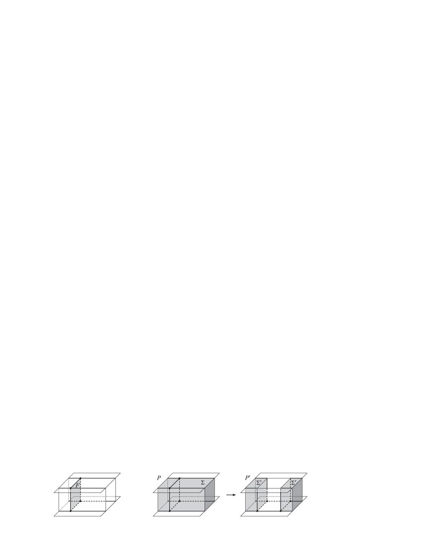
Figure 9: If a face $F$ not contained in $\Sigma$ is embedded, we can modify $P$ to a $P^{\prime}$ with $\chi(\Sigma^{\prime})=\chi(\Sigma)+2$.

So we are left to deal with the last case: namely, we suppose that all faces not contained in $\Sigma$ are not embedded. Lemma 4.7 easily implies that, for the boundary of each face not contained in $\Sigma$, we have one the two cases shown in Fig. 10.

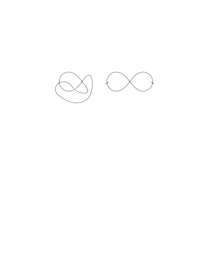
Figure 10: The two cases for the boundary of each face not contained in $\Sigma$ (the dots are vertices of $P$).

Since $p(G)=S(P)$ is connected, the first case is not possible, so we are left to deal with the second one and $p(G)=S(P)$ appears as in Fig. 11-left (we have shown also the neighborhood of the vertices in $\Sigma$).

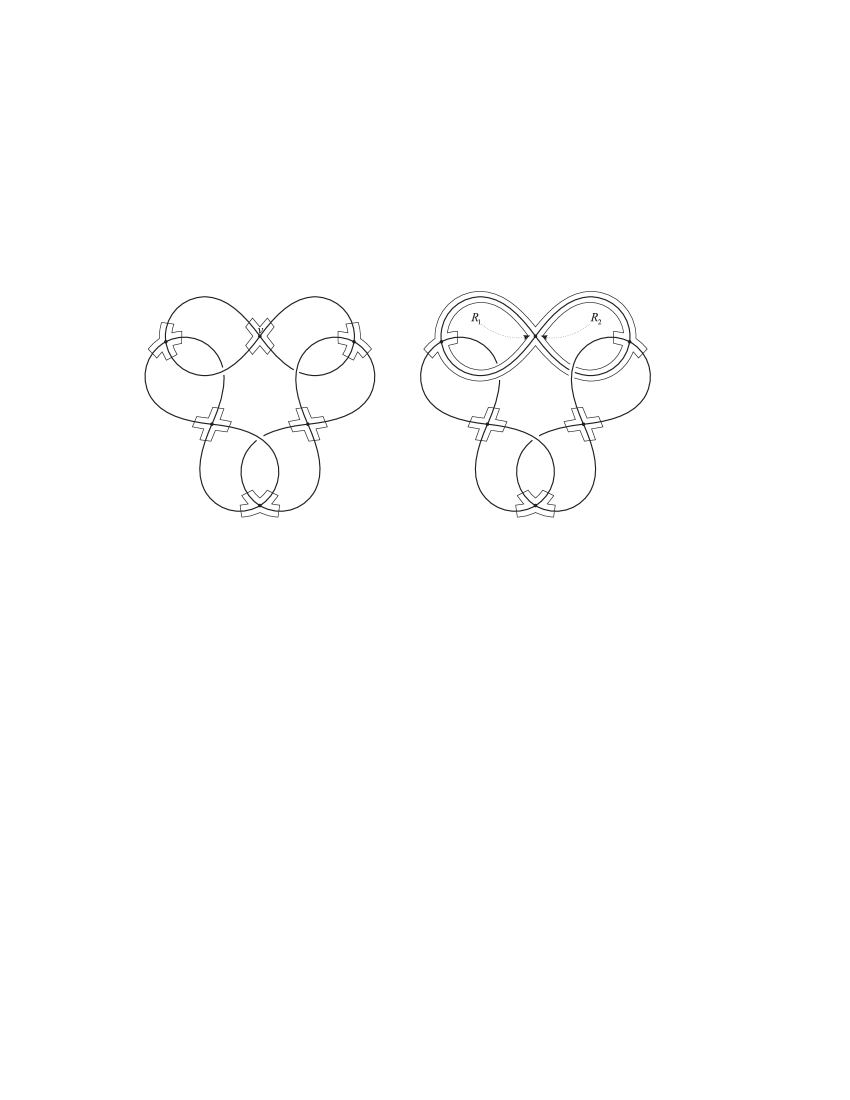
Figure 11: The singular set of $P$ if $\Sigma$ contains only 4-valent vertices (left). Since $\Sigma$ is orientable, we can fix some matchings along the edges (right).

Since $P$ is standard, then, to define $P$ uniquely, it is enough to say how the neighborhoods of the vertices match to each other along the edges. Since $\Sigma$ is orientable, we can suppose (up to symmetry) that, along the edges incident to the vertex $v$, the matchings are those shown in Fig. 11-right. Now, note that all four faces contained in $\Sigma$ are incident to 24 vertices (with multiplicity). For the two faces $R_{1}$ and $R_{2}$, indicated in Fig. 11-right, we have two cases.

If $R_{1}=R_{2}$. The face $R_{1}=R_{2}$ is incident to at least 14 vertices, then the other 3 faces contained in $\Sigma$ are incident to at most $24-14=10$ vertices: a contradiction.

If $R_{1}\neq R_{2}$. Each of the faces $R_{1}$ and $R_{2}$ are incident to at least 10 vertices, so the other 2 faces contained in $\Sigma$ are incident to at most $24-20=4$ vertices: a contradiction.

4.2 Proof of Lemma 1.5

Recall that we want to prove that, if $\Sigma$ consists of two tori, $\mathcal{R}(\Sigma)$ consists of two copies of $T\begin{picture}(12.0,12.0)\put(2.0,0.0){$\times$}\put(2.0,4.5){$\sim$}\end{picture}I$ and each of the components of $\mathcal{R}_{P}(\Sigma)$ appears as shown in Fig. 2. It has been shown at the beginning of the proof of Lemma 1.4 that each component of $\Sigma$ contains 3 vertices of $P$. As said above, there are two interval bundles on the torus up to homeomorphism, namely the orientable $T\times I$ and the non-orientable $T\begin{picture}(12.0,12.0)\put(2.0,0.0){$\times$}\put(2.0,4.5){$\sim$}\end{picture}I$. If a component $\Sigma_{0}$ of $\Sigma$ has an orientable neighborhood, $\partial\mathcal{R}(\Sigma_{0})$ consists of two tori, each containing a component of $G\cap\partial\mathcal{R}(\Sigma_{0})$ with at least two vertices by Lemma 4.3: thus there are at least 4 vertices in $\Sigma_{0}$, a contradiction. Therefore each component of $\Sigma$ has a non-orientable neighborhood.

Let $\Sigma_{0}$ be a component of $\Sigma$. Since $\Sigma_{0}$ contains 3 vertices, Lemma 4.3 implies that $G$ is a $\theta$-graph in the torus $\partial\mathcal{R}(\Sigma_{0})$, and that $p$ maps the $\theta$-graph in $\Sigma_{0}$ producing one 4-valent vertex. It is now easy to show that $\mathcal{R}_{P}(\Sigma_{0})$ appears as shown in Fig. 2, so we leave it to the reader.

4.3 Proof of Lemma 1.6

Recall that we are analyzing the case when $\Sigma$ is one torus and $\mathcal{R}(\Sigma)$ is the orientable $T\times I$, and we want to prove that $\mathcal{R}_{P}(\Sigma)$ appears as in Fig 3. Lemma 4.4 implies that $G$ contains at most $6-1$ vertices, hence it contains 0, 2 or 4 vertices (being 3-valent). Now, since $\mathcal{R}(\Sigma)$ is orientable $G$ has two components. It follows from Lemma 4.3 that $G$ consists of two $\theta$-graphs, each mapped injectively into a $\theta$-graph in $\Sigma$. Two $\theta$-graphs in a torus intersect transversely in at least two points, and they intersect in exactly two only if they share two slopes, i.e. if they are either isotopic or related by a flip. Therefore $\mathcal{R}_{P}(\Sigma)$ is one of the polyhedra shown in Fig. 3.

4.4 Proof of Lemma 1.7

Recall that we are analyzing the case when $\Sigma$ is one torus and $\mathcal{R}(\Sigma)$ is the non-orientable $T\begin{picture}(12.0,12.0)\put(2.0,0.0){$\times$}\put(2.0,4.5){$\sim$}\end{picture}I$, and we want to prove that $M$ has a minimal standard spine with a Stiefel-Whitney surface $\Sigma$ such that $\mathcal{R}(\Sigma)=T\begin{picture}(12.0,12.0)\put(2.0,0.0){$\times$}\put(2.0,4.5){$\sim$}\end{picture}I$ and $\mathcal{R}_{P}(\Sigma)$ is as shown in Fig. 2. As above, Lemma 4.4 implies that $G$ contains at most $6-1$ vertices, hence it contains 0, 2 or 4 vertices (being 3-valent). It follows from Lemma 4.3 that $G$ contains 2 or 4 vertices. If $G$ contains 2 vertices, then it is a $\theta$-graph in the torus $\partial\mathcal{R}(\Sigma)$. Therefore $M$ is obtained assembling $\mathcal{R}(\Sigma)$ and $N=M\setminus\mathcal{R}(\Sigma)$, each manifold having one torus boundary component marked with $G$. Moreover, $\mathcal{R}_{P}(\Sigma)$ and $Q={\rm Cl}(P\setminus\mathcal{R}_{P}(\Sigma))$ are skeleta for $\mathcal{R}(\Sigma)$ and $N$. Since $N$ is not a solid torus, Proposition 2.2 shows that $c(N)\geqslant 3$, thus $Q$ contains at least 3 vertices, hence $\Sigma$ contains at most 3 vertices. As in the proof of Lemma 1.5, we deduce that $\mathcal{R}(\Sigma)$ appears as shown in Fig. 2.

If $G$ contains 4 vertices

To conclude the proof, we show that if $G$ contains 4 vertices, then we can modify $P$ to another spine $P^{\prime}$ of $M$ with the same number of vertices of $P$, with $\Sigma^{\prime}\subset P^{\prime}$ being a torus again, such that $\mathcal{R}(\Sigma^{\prime})=T\begin{picture}(12.0,12.0)\put(2.0,0.0){$\times$}\put(2.0,4.5){$\sim$}\end{picture}I$ and $G^{\prime}$ contains two vertices. Then the conclusion follows from the discussion above.

By applying Lemma 4.3 we get that $\partial\mathcal{R}(\Sigma)\setminus G$ is made of two open discs (say $D$ and $D^{\prime}$). Let us denote by, respectively, $e(D)$ and $e(D^{\prime})$ the number of their edges (with multiplicity). We have $e(D)+e(D^{\prime})=12$, and we suppose $e(D)\leqslant e(D^{\prime})$, so $e(D)\leqslant 6$. Consider the polyhedron $P\cup D$. Then $M\setminus(P\cup D)$ consists of two balls, one of them lying inside $\mathcal{R}(\Sigma)$. For each edge $s$ of $\partial D$, define $f_{s}$ to be the face of $P\cup D$ incident to $s$ and contained in $\mathcal{R}(\Sigma)$. If $s$ has distinct endpoints $q_{0},q_{1}$, then $f_{s}$ is incident to 4 distinct vertices $q_{0},q_{1},p(q_{0}),p(q_{1})$ of $P\cup D$. Now $(P\cup D)\setminus f_{s}$ is another spine of $M$ with $4-e(D)$ vertices less than $P$, hence $e(D)\geqslant 4$ (using that $D$ is embedded if $e(D)\leqslant 4$). If $e(D)=4$, the spine $(P\cup D)\setminus f_{s}$ is standard and minimal, and the new $G^{\prime}$ has two vertices only.

Figure 12: The only possibility for $G$ with $e(D)>4$ (left), the loop $\alpha$ bounding a disc in $M\setminus P$ (centre), and a perturbation of $D$ into $D_{*}$ so that 3 vertices of $\partial D_{*}$ are adjacent to $f_{e_{i}}$ (right).

There is only one case with $e(D)>4$, shown in Fig. 12-left (we have $e(D)=e(D^{\prime})=6$). Set $f_{1}=f_{s_{1}},f_{2}=f_{s_{2}}$. Each $f_{i}$ separates the two balls given by $M\setminus(P\cup D)$. and is incident to at least two vertices of $\Sigma$. If each $f_{i}$ is incident only twice, then $p(s_{1}\cup s_{2})$ does not contain any 4-valent vertex. The loop $\alpha\subset\partial\mathcal{R}(\Sigma)$ shown in Fig. 12-centre then projects to a simple loop $p(\alpha)$ in $\Sigma\setminus p(G)$ which bounds a disc in the ball $M\setminus P$ and meets $p(G)$ in one point, which is absurd (since $P$ is minimal). Therefore some $f_{i}$ is incident to at least 3 vertices of $p(G)$, for $i=1$ or $2$. The disc $D$ is not embedded, so we perturb it into an embedded $D_{*}$. We can do it so that 3 vertices of $\partial D_{*}$ are adjacent to $f_{i}$ (with a perturbation depending on $i$, see Fig. 12-right), thus $f_{i}$ is incident to at least 6 distinct vertices of $P\cup D_{*}$.

If $f_{i}$ is incident to more than 6 vertices, then $(P\cup D_{*})\setminus f_{i}$ is a standard spine of $M$ with less vertices than $P$. Therefore $f_{i}$ is incident to exactly 6 vertices and $(P\cup D_{*})\setminus f_{i}$ is the required minimal standard spine of $M$ (with the same number of vertices of $P$), with a new $G^{\prime}$ having 2 vertices.

Dipartimento di Matematica
                                                         Università di Pisa
                                                         Via F. Buonarroti 2
                                                         56127 Pisa, Italy
                                                         amendola@mail.dm.unipi.it
                                                         martelli@mail.dm.unipi.it

References

- [1] P. J. Callahan – M. V. Hildebrand – J. R. Weeks, A census of cusped hyperbolic -manifolds. Mathematics of Computation 68 (1999), 321-332.
- [2] W. Floyd – A. Hatcher, Incompressible surfaces in punctured torus bundles, Topology Appl. 13 (1982), 263-282.
- [3] R. Frigerio – B. Martelli – C. Petronio Low-complexity hyperbolic manifolds with geodesic boundary, in preparation.
- [4] J. C. Gómez-Larrañaga – W. Heil – V. Núñez, Stiefel-Whitney surfaces and decompositions of 3-manifolds into handlebodies, Topology Appl. 60 (1995), 267-280.
- [5] B. Martelli – C. Petronio, Three-manifolds having complexity at most , Experiment. Math. 10 (2001), 207-237.
- [6] B. Martelli – C. Petronio, A new decomposition theorem for -manifolds, Math.GT/0105034, to appear in Illinois J. Math.
- [7] S. V. Matveev, Complexity theory of three-dimensional manifolds, Acta Appl. Math. 19 (1990), 101-130.
- [8] S. V. Matveev - A. T. Fomenko, Constant energy surfaces of Hamiltonian systems, enumeration of three-dimensional manifolds in increasing order of complexity, and computation of volumes of closed hyperbolic manifolds. Russ. Math. Surv. 43 (1988), 3-25.
- [9] P. Scott, The geometries of -manifolds, Bull. London Math. Soc. 15 (1983), 401-487.
- [10] http://www.dm.unipi.it/pages/petronio/