Spectral Flow, Maslov Index and
Bifurcation of semi-Riemannian Geodesics

Abstract.

We give a functional analytical proof of the equality between the Maslov index of a semi-Riemannian geodesic and the spectral flow of the path of self-adjoint Fredholm operators obtained from the index form. This fact, together with recent results on the bifurcation for critical points of strongly indefinite functionals (see [3]) imply that each non degenerate and non null conjugate (or $P$-focal) point along a semi-Riemannian geodesic is a bifurcation point.

1. Introduction

Let $(M,g)$ be a semi-Riemannian manifold and $p\in M$; a point $q\in M$ is conjugate to $p$ if $q$ is a critical value of the exponential map $\exp_{p}$, i.e., if the linearized geodesic map $\mathrm{d}\exp_{p}$ is not injective at $\exp_{p}^{-1}(q)$. It is a natural question to ask whether the non injectivity at the linear level implies non uniqueness of geodesics between two conjugate points. For instance, two antipodal points on the Riemannian round sphere are joined by infinitely many geodesics; however, it is easy to produce examples of conjugate points in complete Riemannian manifolds that are joined by a unique geodesic.

In order to make a more precise sense of the above question, first one has to observe that any information obtained from the linearized geodesic equation can only be of local character, which implies that one should not expect to detect the existence of a finite number of geodesics between two points along $\gamma$ by merely looking at the Jacobi equation. A similar situation occurs, for instance, when studying cut points along a Riemannian geodesic, that are not necessarily related to conjugate points. On the other hand, in a number of situations it is desirable to have a better picture of the geodesic behavior near a conjugate point, and in order to investigate this situation we introduce the notion of bifurcation point:

Definition.

Let $(M,g)$ be a semi-Riemannian geodesic, $\gamma:[a,b]\to M$ be a geodesic in $M$ and $t_{0}\in\left]a,b\right[$. The point $\gamma(t_{0})$ is said to be a bifurcation point for $\gamma$ (see Figure 1) if there exists a sequence $\gamma_{n}:[a,b]\to M$ of geodesics in $M$ and a sequence $(t_{n})_{n\in I\!\!N}\subset\left]a,b\right[$ satisfying the following properties:

1. $\gamma_{n}(a)=\gamma(a)$ for all $n$;

2. $\gamma_{n}(t_{n})=\gamma(t_{n})$ for all $n$;

3. $\gamma_{n}\to\gamma$ as $n\to\infty$;

4. $t_{n}\to t_{0}$ (and thus $\gamma_{n}(t_{n})\to\gamma(t_{0})$) as $n\to\infty$.

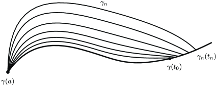
Figure 1. Bifurcation of geodesics.

The convergence of geodesics in condition (3) is meant in any reasonable sense, for instance, it suffices to require that $\dot{\gamma}_{n}(a)\to\dot{\gamma}(a)$ as $n\to\infty$.

Using the Implicit Function Theorem, it follows immediately from the above Definition that if $\gamma(t_{0})$ is a bifurcation point for $\gamma$, then necessarily $\gamma(t_{0})$ must be conjugate to $\gamma(a)$ along $\gamma$. It is interesting to observe here that the above definition of bifurcation point along a geodesic has strong analogies with Jacobi’s original definition of conjugate point along an extremal of quadratic functionals (see for instance [4, Definition 4, p. 114]).

The definition of bifurcation point is well understood with the example of the paraboloid $z=x^{2}+y^{2}$, endowed with the Euclidean metric of $I\!\!R^{3}$ (see Figure 2).

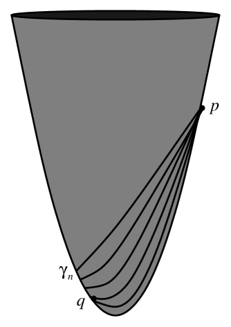
Figure 2. Geodesics issuing at a point $p$ of the paraboloid, tending to the meridian through $p$.

Consider in this case the geodesic $\gamma$ given by the meridian issuing from a point $p$ distinct from the vertex of the paraboloid, with initial velocity pointing in the negative $z$ direction. Such meridian goes downward towards the vertex, and then up again towards infinite on the opposite side of the paraboloid; this geodesic has a (unique) conjugate point $q$, and neighboring geodesics starting at $p$ intersect the meridian at points $q_{n}\neq q$ that tend to $q$, and thus $q$ is a bifurcation point along $\gamma$.

Under the light of the above Definition, we reformulate the non uniqueness geodesic problem as follows: which conjugate points along a semi-Riemannian geodesic are bifurcation points? Several other bifurcation questions are naturally associated to semi-Riemannian geometry. For instance, one could replace the notion of conjugate point by that of focal point along a geodesic $\gamma$ relatively to an initial submanifold $P$ of $M$, and could ask which $P$-focal points are limits of endpoints of geodesics starting orthogonally at $P$ and terminating on $\gamma$.

In this paper we use some recent results on bifurcation theory for strongly indefinite functionals ([3]) and on symplectic techniques for semi-Riemannian geodesics ([9, 10, 11]) to give an answer to the above questions. We outline briefly the ideas behind the theory of Fitzpatrick, Pejsachowicz and Recht and how their result is employed in the present paper. The most classical result on variational bifurcation (see [5]) states that bifurcation for a smooth path of functionals having a trivial branch of critical points with finite Morse index (assumed nondegenerate at the endpoints) occurs at a given singular critical point if such singular point determines a jump of the Morse index. The variation of the Morse index at the endpoints of a path of essentially positive self-adjoint Fredholm operators is a homotopy invariant of the path; recall to this aim that the space of essentially positive self-adjoint Fredholm operators form a contractible space, and that the invertible ones have an infinite number of connected components, which are labelled by the Morse index. When dealing with strongly indefinite self-adjoint Fredholm operators, then the topology of the space becomes richer (fundamental group isomorphic to $\mathbb{Z}$), and no homotopy invariant for paths can be defined by simply looking at the endpoints of the path. The spectral flow for a path, originally introduced by Atiyah, Patodi and Singer (see [2]), is an integer valued invariant associated to paths of this type, and it is given, roughly speaking, by a signed count of the eigenvalues that pass through zero at each singular instants. The main result in [3] is that bifurcation occurs at those singular instants whose contribution to the spectral flow is non null (See Proposition 3.2 below).

Consider now the geodesic bifurcation problem mentioned above. By a suitable choice of coordinates in the space of paths joining a fixed point $p$ in $M$ and a point variable along a given geodesic $\gamma$ starting at $p$, the geodesic bifurcation problem is reduced to a bifurcation problem for a smooth family of strongly indefinite functionals defined in (an open neighborhood of $0$ of) a fixed Hilbert space. The path of Fredholm operators corresponding to the index form along the geodesic is studied, and the main result of our computations is that its spectral flow coincides, up to a sign, with another well known integer valued invariant of the geodesic, called the Maslov index. Under a certain nondegeneracy assumption, the Maslov index is computed as the sum of the signatures of all conjugate points along the geodesic. Applying the theory of [3], we get that nondegenerate conjugate points with non vanishing signature are bifurcation points; more generally, a bifurcation points is found in every segment of geodesic that contains a (possibly non discrete) set of conjugate points that give a non zero contribution to the Maslov index. In particular, Riemannian conjugate points are always bifurcation points, as well as conjugate points along timelike or lightlike Lorentzian geodesics. Similar results hold for focal points to an initial nondegenerate submanifold.

2. Fredholm bilinear forms on Hilbert spaces

In this section we will discuss the notion of index of a Fredholm bilinear form on a Hilbert space relatively to a closed subspace. The main goal (Proposition 2.5) is a result that gives the relative index of a form to the difference between the index and the coindex of suitable restrictions of the form.

2.1. On the relative index of Fredholm forms

Let $H$ be a Hilbert space with inner product $\langle\cdot,\cdot\rangle$, and let $B$ a bounded symmetric bilinear form on $H$; there exists a unique self-adjoint bounded operator $S:H\to H$ such that $B=\langle S\cdot,\cdot\rangle$, that will be called the realization of $B$ (with respect to $\langle\cdot,\cdot\rangle$). $B$ is nondegenerate if its realization is injective, $B$ is strongly nondegenerate if $S$ is an isomorphism. If $B$ is strongly nondegenerate, or if more generally $0$ is not an accumulation point of the spectrum of $S$, we will call the negative space (resp., the positive space) of $B$ the closed subspace $V^{\scriptscriptstyle-}(S)$ (resp., $V^{\scriptscriptstyle+}(S)$) of $H$ given by $\chi_{\left]-\infty,0\right[}(S)$ (resp., $\chi_{\left]0,+\infty\right[}(S)$), where $\chi_{I}$ denotes the characteristic function of the interval $I$. We will say that $B$ is Fredholm if $S$ is Fredholm, or that $B$ is RCPPI, realized by a compact perturbation of a positive isomorphism, (resp., RCPNI) if $S$ is of the form $S=P+K$ (resp., $S=N+K$) where $P$ is a positive isomorphism of $H$ ($N$ is a negative isomorphism of $H$) and $K$ is compact. Observe that the properties of being Fredholm, RCPPI or RCPNI do not depend on the inner product, although the realization $S$ and the spaces $V^{\pm}(S)$ do.

The index (resp., the coindex) of $B$, denoted by $n_{-}(B)$ (resp., $n_{+}(B)$) is the dimension of $V^{\scriptscriptstyle-}(S)$ (resp., of $V^{\scriptscriptstyle+}(S)$); the nullity of $B$, denoted by $n_{0}(B)$ is the dimension of the kernel of $S$.

If $B$ is RCPPI (resp., RCPNI), then both its nullity $n_{0}(B)$ and its index $n_{-}(B)$ (resp., and its coindex $n_{+}(B)$) are finite numbers.

Given a closed subspace $W\subset H$, the $B$-orthogonal complement of $W$, denoted by $W^{\perp_{B}}$, is the closed subspace of $H$:

$$W^{\perp_{B}}=\big{\{}x\in H:B(x,y)=0\ \text{for all}\ y\in W\big{\}};$$

clearly,

$$W^{\perp_{B}}=S^{-1}(W^{\perp}).$$

If $B$ is Fredholm, $S$ is its realization and $W\subset H$ is any subspace, then the following properties hold:

1. $B$ is nondegenerate iff it is strongly nondegenerate;

2. $n_{0}(B)<+\infty$;

3. $(W^{\perp_{B}})^{\perp_{B}}=\overline{W}+\mathrm{Ker}(S)$;

4. if $W$ is closed, then $W+W^{\perp_{B}}$ is closed;

5. if $W$ is closed and $B|_{W}$ (i.e., the restriction of $B$ to $W\times W$) in nondegenerate, then also $B|_{W^{\perp_{B}}}$ is nondegenerate and $H=W\oplus W^{\perp_{B}}$.

Let us now recall a few basic things on the notion of commensurability of closed subspaces (see reference [1] for more details). Let $V,W\subset H$ be closed subspaces and let $P_{V}$ and $P_{W}$ denote the orthogonal projections respectively onto $V$ and $W$. We say that $V$ and $W$ are commensurable if $P_{V}-P_{W}$ is a compact operator. Equivalently, $V$ and $W$ are commensurable if both $P_{W^{\perp}}P_{V}$ and $P_{V^{\perp}}P_{W}$ are compact; if $V$ and $W$ are commensurable the relative dimension $\mathrm{dim}_{V}(W)$ of $W$ with respect to $V$ is defined as:

$$\mathrm{dim}_{V}(W)=\mathrm{dim}(W\cap V^{\perp})-\mathrm{dim}(W^{\perp}\cap V).$$

Clearly, if $V$ and $W$ are commensurable, then $V^{\perp}$ and $W^{\perp}$ are commensurable, and:

$$\mathrm{dim}_{V^{\perp}}(W^{\perp})=-\mathrm{dim}_{V}(W).$$

The notion of commensurability of subspaces does not depend on the Hilbert space inner product of $H$.

Proposition 2.1.

Let $S,T$ be linear bounded self-adjoint operators on $H$ whose difference $K=S-T$ is compact. Then $V^{\scriptscriptstyle-}(S)$ (resp., $V^{\scriptscriptstyle+}(S)$) is commensurable with $V^{\scriptscriptstyle-}(T)$ (resp., with $V^{\scriptscriptstyle+}(T)$).

Conversely, assume that $S$ is a bounded self-adjoint Fredholm operator on $H$, and let $H=W^{\scriptscriptstyle-}\oplus W^{\scriptscriptstyle+}$ be an orthogonal decomposition of $H$ such that $W^{\scriptscriptstyle-}$ is commensurable with $V^{\scriptscriptstyle-}(S)$ and $W^{\scriptscriptstyle+}$ is commensurable with $V^{\scriptscriptstyle+}(S)$. Then there exists an invertible self-adjoint operator $T$ on $H$ such that $V^{\scriptscriptstyle-}(T)=W^{\scriptscriptstyle-}$, $V^{\scriptscriptstyle+}(T)=W^{\scriptscriptstyle+}$ and such that $S-T$ is compact.

Proof.

See [1, Proposition 2.3.2 and Proposition 2.3.5]. ∎

Lemma 2.2.

Let $B$ be a Fredholm symmetric bilinear form on the Hilbert space $H$ and let $W\subset H$ be a closed subspace. Then, the following are equivalent:

• $B|_{W}$ is RCPNI and $B|_{W^{\perp_{B}}}$ is RCPPI;

• there exists a Hilbert space inner product $\langle\cdot,\cdot\rangle$ on $H$ such that $W$ is commensurable with $V^{\scriptscriptstyle-}(S)$, where $S$ is the realization of $B$ with respect to $\langle\cdot,\cdot\rangle$.

Proof.

Assume that (b) holds; fix a Hilbert space inner product $\langle\cdot,\cdot\rangle$ in $H$ and let $S$ be the realization of $B$ with respect to $\langle\cdot,\cdot\rangle$ so that $W$ is commensurable with $V^{\scriptscriptstyle-}(S)$. Then $W^{\perp}$ is commensurable with $V^{\scriptscriptstyle-}(S)^{\perp}=V^{\scriptscriptstyle+}(S)\oplus\mathrm{Ker}(B)$. Moreover, since $\mathrm{Ker}(B)$ is finite dimensional, then $W^{\perp}$ is also commensurable with $V^{\scriptscriptstyle+}(S)$. By Proposition 2.1, there exists an invertible self-adjoint operator $T:H\to H$ such that $V^{\scriptscriptstyle-}(T)=W$, $V^{\scriptscriptstyle+}(T)=W^{\perp}$, and with $S=T+K$, with $K$ compact. It follows easily that $B|_{W}$ is RCPNI (namely, if $P$ denotes the orthogonal projection onto $W$, the realization of $B|_{W}$ is $PS|_{W}=(PT+PK)|_{W}=(T+PK)|_{W}$), and $B|_{W^{\perp}}$ is RCPPI. Observe in particular that $W\cap W^{\perp_{B}}=\mathrm{Ker}(B|_{W})$ is finite dimensional. To prove that $B|_{W^{\perp_{B}}}$ is RCPPI we argue as follows; denote by $P$ the orthogonal projection onto $W$ and by $P^{\scriptscriptstyle\perp}=1-P$ the orthogonal projection onto $W^{\perp}$. As we have observed, $W^{\perp_{B}}=S^{-1}(W^{\perp})$; hence, for all $x,y\in W^{\perp_{B}}$ we have:

(2.1) $$\begin{split}B(x,y)&\,=\langle Sx,y\rangle=\langle Sx,P^{\scriptscriptstyle\perp}y\rangle=\langle SPx,P^{\scriptscriptstyle\perp}y\rangle+\langle SP^{\scriptscriptstyle\perp}x,P^{\scriptscriptstyle\perp}y\rangle=\\ &\,=\langle P^{\scriptscriptstyle\perp}KPx,y\rangle+\langle P^{\scriptscriptstyle\perp}TP^{\scriptscriptstyle\perp}x,y\rangle+\langle P^{\scriptscriptstyle\perp}KP^{\scriptscriptstyle\perp}x,y\rangle.\end{split}$$

In the above equality we have used the fact that $W$ and $W^{\perp}$ are $T$-invariant. From (2.1) we deduce that $B|_{W^{\perp_{B}}}$ is represented by a compact perturbation of the operator $\widetilde{T}:W^{\perp_{B}}\to W^{\perp_{B}}$ given by $\widetilde{T}=P^{\scriptscriptstyle\perp_{B}}P^{\scriptscriptstyle\perp}TP^{\scriptscriptstyle\perp}|_{W^{\perp_{B}}}$ (where $P^{\scriptscriptstyle\perp_{B}}$ is the orthogonal projection onto $W^{\perp_{B}}$) which is positive semi-definite. The kernel of $\widetilde{T}$ is easily computed as the finite dimensional space $W^{\perp_{B}}\cap T^{-1}\big{(}W\cap W^{\perp_{B}}\big{)}$; it follows that $\widetilde{T}$ is a compact perturbation of a positive isomorphism of $W^{\perp_{B}}$, which proves that (b) implies (a).

Conversely, if $B|_{W}$ is RCPNI and $B|_{W^{\perp_{B}}}$ is RCPPI, then clearly $W_{1}=W\cap W^{\perp_{B}}$ is finite dimensional; let $\widetilde{W}$ be any closed complement of $W_{1}$ in $W$. It follows that $B|_{\widetilde{W}}$ is nondegenerate, which implies that we have a direct sum decomposition $H=\widetilde{W}\oplus\widetilde{W}^{\perp_{B}}$. If $\langle\cdot,\cdot\rangle$ is any Hilbert space inner product for which $\widetilde{W}$ and $\widetilde{W}^{\perp_{B}}$ are orthogonal, then it is easily checked that the corresponding realization $S$ of $B$ is such that $V^{\scriptscriptstyle-}(S)$ is commensurable with $W$.

This concludes the proof. ∎

Assume now that $B$ is a symmetric bilinear form, $S$ is its realization; if $W$ is closed subspace of $H$ which is commensurable with $V^{\scriptscriptstyle-}(S)$, the one defines the relative index of $B$ with respect to $W$, denoted by $\mathrm{ind}_{W}(B)$, the integer number:

$$\mathrm{ind}_{W}(B)=\mathrm{dim}_{W}\big{(}V^{\scriptscriptstyle-}(S)\big{)}.$$

Again, the relative index is independent of the inner product, and the following equality holds:

$$\mathrm{ind}_{W}(B)=\sup\big{\{}\mathrm{dim}_{W}(V):V\ \text{is commensurable with}\ V^{\scriptscriptstyle-}(S)\big{\}}.$$

2.2. Computation of the relative index

A subspace $Z$ of $H$ is said to be isotropic for the symmetric bilinear form $B$ of $B|_{Z}\equiv 0$.

Lemma 2.3.

Let $B$ be a RCPPI symmetric bilinear form on $H$, and let $Z\subset H$ be an isotropic subspace of $B$. Then:

$$n_{-}(B)=n_{-}\big{(}B|_{Z^{\perp_{B}}}\big{)}+\mathrm{dim}(Z).$$

Proof.

Since $B$ is RCPPI, then the index $n_{-}(B)$ is finite, and so $n_{-}\big{(}B|_{Z^{\perp_{B}}}\big{)}$ and $\mathrm{dim}(Z)$ are finite. Clearly, $Z\subset Z^{\perp_{B}}$; let $U\subset Z^{\perp_{B}}$ be a closed subspace such that $Z^{\perp_{B}}=Z\oplus U$, so that $B|_{U}$ is nondegenerate and $H=U\oplus U^{\perp_{B}}$. Moreover:

$$n_{-}(B)=n_{-}\big{(}B|_{U}\big{)}+n_{-}\big{(}B|_{U^{\perp_{B}}}\big{)}.$$

Since $Z$ is isotropic, then $n_{-}\big{(}B|_{U}\big{)}=n_{-}\big{(}B|_{Z^{\perp_{B}}}\big{)}$; to conclude the proof we need to show that $n_{-}\big{(}B|_{U^{\perp_{B}}}\big{)}=\mathrm{dim}(Z)$. To this aim, observe first that $\mathrm{dim}(U^{\perp_{B}})=2\mathrm{dim}(Z)$. Namely, $\mathrm{dim}(U^{\perp_{B}})=\mathrm{codim}(U)$; moreover, $\mathrm{codim}_{Z^{\perp_{B}}}(U)=\mathrm{dim}(Z)$, and $\mathrm{codim}(Z^{\perp_{B}})=\mathrm{dim}(Z)$. Thus, keeping in mind that the dimension of an isotropic subspace is less than or equal to the index and the coindex, we have:

$$n_{-}\big{(}B|_{U^{\perp_{B}}}\big{)}+n_{+}\big{(}B|_{U^{\perp_{B}}}\big{)}=\mathrm{dim}(U^{\perp_{B}})=2\,\mathrm{dim}(Z)\leq n_{-}\big{(}B|_{U^{\perp_{B}}}\big{)}+n_{+}\big{(}B|_{U^{\perp_{B}}}\big{)},$$

which proves that $n_{-}\big{(}B|_{U^{\perp_{B}}}\big{)}=n_{+}\big{(}B|_{U^{\perp_{B}}}\big{)}=\mathrm{dim}(Z)$ and concludes the proof. ∎

Lemma 2.4.

Let $B$ be a nondegenerate Fredholm symmetric bilinear form on $H$ and $W\subset H$ be a closed subspace such that $B|_{W^{\perp_{B}}}$ is RCPPI. Let $\widetilde{W}$ be any closed complement of $W\cap W^{\perp_{B}}$ in $W$. Then the following identity holds:

$$n_{-}\big{(}B|_{\widetilde{W}^{\perp_{B}}}\big{)}=n_{-}\big{(}B|_{W^{\perp_{B}}}\big{)}+\mathrm{dim}\big{(}W\cap W^{\perp_{B}}\big{)}.$$

Proof.

We start with the observation that $\mathrm{Ker}\big{(}B|_{W}\big{)}=\mathrm{Ker}\big{(}B|_{W^{\perp_{B}}}\big{)}=W\cap W^{\perp_{B}}$; this implies in particular that $B|_{\widetilde{W}}$ and $B|_{\widetilde{W}^{\perp_{B}}}$ are nondegenerate. Since $B|_{W^{\perp_{B}}}$ is RCPPI, then $n_{-}\big{(}B|_{W^{\perp_{B}}}\big{)}$ and $\mathrm{dim}(W\cap W^{\perp_{B}})=n$ are finite numbers.

Since $\mathrm{codim}_{\widetilde{W}^{\perp_{B}}}\big{(}W^{\perp_{B}}\big{)}=n$, then:

$$n_{-}\big{(}B|_{\widetilde{W}^{\perp_{B}}}\big{)}\leq n_{-}\big{(}B|_{W^{\perp_{B}}}\big{)}+n,$$

from which it follows that $n_{-}\big{(}B|_{\widetilde{W}^{\perp_{B}}}\big{)}$ is finite; moreover, $B|_{\widetilde{W}^{\perp_{B}}}$ is RCPPI. The conclusion now follows easily from Lemma 2.3, applied to the bilinear form $B|_{\widetilde{W}^{\perp_{B}}}$ and the isotropic space $Z=W\cap W^{\perp_{B}}$. ∎

We are finally ready to give our central result concerning the computation of the relative index of a Fredholm bilinear form $B$ in terms of index and coindex of suitable restrictions of $B$:

Proposition 2.5.

Let $B$ be a Fredholm symmetric bilinear form on $H$, $S$ its realization and let $W\subset H$ be a closed subspace which is commensurable with $V^{\scriptscriptstyle-}(S)$. Then the relative index $\mathrm{ind}_{W}(B)$ is given by:

(2.2) $$\mathrm{ind}_{W}(B)=n_{-}\big{(}B|_{W^{\perp_{B}}}\big{)}-n_{+}\big{(}B|_{W}\big{)}.$$

Proof.

Assume first that $B$ is nondegenerate on $W$; then have a direct sum decomposition $H=W\oplus W^{\perp_{B}}$. The relative $\mathrm{ind}_{W}(B)$ does not change if we change the inner product of $H$; we can therefore assume that $W$ and $W^{\perp_{B}}$ are orthogonal subspaces of $H$. Then, $S=S^{\scriptscriptstyle-}\oplus S^{\scriptscriptstyle+}$, where $S^{\scriptscriptstyle-}:W\to W$ is the realization of $B|_{W}$ and $S^{\scriptscriptstyle+}:W^{\perp_{B}}\to W^{\perp_{B}}$ is the realization of $B|_{W^{\perp_{B}}}$. Moreover, $V^{\scriptscriptstyle-}(S)=V^{\scriptscriptstyle-}(S^{\scriptscriptstyle-})\oplus V^{\scriptscriptstyle-}(S^{\scriptscriptstyle+})$. An immediate calculation yields:

$$\begin{split}\mathrm{ind}_{W}(B)\,&=\mathrm{dim}\big{(}V^{\scriptscriptstyle-}(S)\cap W^{\perp_{B}}\big{)}-\mathrm{dim}\big{(}V^{\scriptscriptstyle-}(S)^{\perp}\cap W\big{)}\\ &=\mathrm{dim}\big{(}V^{\scriptscriptstyle-}(S)\cap W^{\perp_{B}}\big{)}-\mathrm{codim}_{W}\big{(}V^{\scriptscriptstyle-}(S^{\scriptscriptstyle-})\big{)}\\ &=\mathrm{dim}\big{(}V^{\scriptscriptstyle-}(S^{\scriptscriptstyle+})\big{)}-\mathrm{codim}_{W}\big{(}V^{\scriptscriptstyle-}(S^{\scriptscriptstyle-})\big{)}\\ &=n_{-}\big{(}B|_{W^{\perp_{B}}}\big{)}-n_{+}\big{(}B|_{W}\big{)}.\end{split}$$

Let us consider now the case that $B|_{W}$ is degenerate; by Lemma 2.2, $B|_{W}$ is RCPNI, and so $\mathrm{dim}\big{(}W\cap W^{\perp_{B}}\big{)}=n<+\infty$. Set $\widetilde{W}=\big{(}W\cap W^{\perp_{B}}\big{)}^{\perp}\cap W$, so that $B|_{\widetilde{W}}$ is nondegenerate; moreover, $V^{\scriptscriptstyle-}(S)$ is commensurable with $\widetilde{W}$, because it has finite codimension in $W$. We can then apply the first part of the proof, and we obtain:

(2.3) $$\mathrm{ind}_{\widetilde{W}}(B)=n_{-}\big{(}B|_{\widetilde{W}^{\perp_{B}}}\big{)}-n_{+}\big{(}B|_{\widetilde{W}}\big{)}.$$

Clearly,

(2.4) $$n_{+}\big{(}B|_{\widetilde{W}}\big{)}=n_{+}\big{(}B|_{W}\big{)};$$

moreover, by definition of relative index:

(2.5) $$\mathrm{ind}_{\widetilde{W}}(B)=\mathrm{ind}_{W}(B)+n.$$

Finally, by Lemma 2.2, $B|_{W^{\perp_{B}}}$ is RCPPI, and by Lemma 2.4:

(2.6) $$n_{-}\big{(}B|_{\widetilde{W}^{\perp_{B}}}\big{)}=n_{-}\big{(}B|_{W^{\perp_{B}}}\big{)}+n.$$

Formulas (2.3), (2.4), (2.5) and (2.6) yield (2.2) and conclude the proof. ∎

3. On the spectral flow of a path of self-adjoint Fredholm operators

In this section we will recall some facts from the theory of variational bifurcation for strongly indefinite functionals. The basic reference for the material presented is [3]; as to the definition and the basic properties of the spectral flow we refer to the nice article by Phillips [8], from which we will borrow some of the notations.

3.1. Spectral flow

Let us consider an infinite dimensional separable real Hilbert space $H$. We will denote by $\mathcal{B}(H)$ and $\mathcal{K}(H)$ respectively the algebra of all bounded linear operators on $H$ and the closed two-sided ideal of $\mathcal{B}(H)$ consisting of all compact operators on $H$; the Calkin algebra $\mathcal{B}(H)/\mathcal{K}(H)$ will be denoted by $\mathcal{Q}(H)$, and $\pi:\mathcal{B}(H)\to\mathcal{Q}(H)$ will denote the quotient map. The essential spectrum $\sigma_{\!\scriptscriptstyle{\textrm{ess}}}(T)$ of a bounded linear operator $T\in\mathcal{B}(H)$ is the spectrum of $\pi(T)$ in the Calkin algebra $\mathcal{Q}(H)$. Let $\mathcal{F}(H)$ and $\mathcal{F}^{\scriptscriptstyle{\textrm{sa}}}(H)$ denote respectively the space of all Fredholm (bounded) linear operators on $H$ and the space of all self-adjoint ones. An element $T\in\mathcal{F}^{\scriptscriptstyle{\textrm{sa}}}(H)$ is said to be essentially positive (resp., essentially negative) if $\sigma_{\!\scriptscriptstyle{\textrm{ess}}}(T)\subset I\!\!R^{+}$ (resp., if $\sigma_{\!\scriptscriptstyle{\textrm{ess}}}(T)\subset I\!\!R^{-}$), and strongly indefinite if it is neither essentially positive nor essentially negative.

The symbols $\mathcal{F}^{\scriptscriptstyle{\textrm{sa}}}_{+}(H)$, $\mathcal{F}^{\scriptscriptstyle{\textrm{sa}}}_{-}(H)$ and $\mathcal{F}^{\scriptscriptstyle{\textrm{sa}}}_{*}(H)$ will denote the subsets of $\mathcal{F}^{\scriptscriptstyle{\textrm{sa}}}(H)$ consisting respectively of all essentially positive, essentially negative and strongly indefinite self-adjoint Fredholm operators on $H$. These sets are precisely the three connected components of $\mathcal{F}^{\scriptscriptstyle{\textrm{sa}}}(H)$; $\mathcal{F}^{\scriptscriptstyle{\textrm{sa}}}_{+}(H)$ and $\mathcal{F}^{\scriptscriptstyle{\textrm{sa}}}_{-}(H)$ are contractible, while $\mathcal{F}^{\scriptscriptstyle{\textrm{sa}}}_{*}(H)$ is homotopically equivalent to $U(\infty)=\lim_{n}U(n)$, and it has infinite cyclic fundamental group.

Given a continuous path $S:[0,1]\to\mathcal{F}^{\scriptscriptstyle{\textrm{sa}}}_{*}(H)$ with $S(0)$ and $S(1)$ invertible, the spectral flow of $S$, denoted by $\mathrm{sf}(S)$, is an integer number which is given, roughly speaking, by the net number of eigenvalues that pass through zero in the positive direction from the start of the path to its end. There exist several equivalent definitions of the spectral flow in the literature; we like to mention here the definition given in [8] using functional calculus, and that reduces the problem to a simple dimension counting of finite rank projections.

More precisely, let $\chi_{I}$ denote the characteristic function of the interval $I$; for all $S\in\mathcal{F}^{\scriptscriptstyle{\textrm{sa}}}_{*}(H)$ there exists $a>0$ and a neighborhood $U$ of $S$ in $\mathcal{F}^{\scriptscriptstyle{\textrm{sa}}}_{*}(H)$ such that the map $T\mapsto\chi_{[-a,a]}(T)$ is norm continuous in $U$, and it takes values in the set of projections of finite rank. Denote by $C^{0}_{\#}\big{(}[0,1],\mathcal{F}^{\scriptscriptstyle{\textrm{sa}}}_{*}(H)\big{)}$ the set of all continuous paths $S:[0,1]\to\mathcal{F}^{\scriptscriptstyle{\textrm{sa}}}_{*}(H)$ such that $S(0)$ and $S(1)$ are invertible. Given $S\in C^{0}_{\#}\big{(}[0,1],\mathcal{F}^{\scriptscriptstyle{\textrm{sa}}}_{*}(H)\big{)}$, then by the above property one can choose a partition $0=t_{0}<t_{1}<\ldots<t_{N}=1$ of $[0,1]$ and positive numbers $a_{1},\ldots,a_{N}$ such that the maps $t\mapsto\chi_{[-a_{i},a_{i}]}\big{(}S(t)\big{)}$ are continuous and of finite rank on $[t_{i-1},t_{i}]$ for all $i$. The spectral flow of the path $S$ is defined to be the sum:

$$\sum_{i=1}^{n}\Big{[}\mathrm{rk}\big{(}\chi_{[0,a_{i}]}(S(t_{i}))\big{)}-\mathrm{rk}\big{(}\chi_{[0,a_{i}]}(S(t_{i-1}))\big{)}\Big{]},$$

where $\mathrm{rk}$ is the rank of a projection. With the above formula, the spectral flow is well defined, i.e., it does not depend on the choice of the partition $(t_{i})$ and of the positive numbers $(a_{i})$, and the map $\mathrm{sf}:C^{0}_{\#}\big{(}[0,1],\mathcal{F}^{\scriptscriptstyle{\textrm{sa}}}_{*}(H)\big{)}\to\mathbb{Z}$ has the following properties:

• it is additive by concatenation;

• if $S\in C^{0}_{\#}\big{(}[0,1],\mathcal{F}^{\scriptscriptstyle{\textrm{sa}}}_{*}(H)\big{)}$ is such that $S(t)$ is invertible for all $t$, then $\mathrm{sf}(S)=0$;

• it is invariant by homotopies with fixed endpoints;

• the induced map $\mathrm{sf}:\pi_{1}\big{(}\mathcal{F}^{\scriptscriptstyle{\textrm{sa}}}_{*}(H)\big{)}\to\mathbb{Z}$ is an isomorphism.

For the purposes of the present paper, it will be useful to give a different description of the spectral flow, which follows the approach in [3]. As we have observed, $\mathcal{F}^{\scriptscriptstyle{\textrm{sa}}}_{*}(H)$ is not simply connected, and therefore no non trivial homotopic invariant for curves in $\mathcal{F}^{\scriptscriptstyle{\textrm{sa}}}_{*}(H)$ can be defined only in terms of the value at the endpoints. However, in [3] it is shown that the spectral flow can be defined in terms of the endpoints, provided that the path $S$ has the special form $S(t)=\mathfrak{J}+K(t)$, where $\mathfrak{J}$ is a fixed symmetry of $H$ and $t\mapsto K(t)$ is a path of compact operators. By a symmetry of the Hilbert space $H$ it is meant an operator $\mathfrak{J}$ of the form

$$\mathfrak{J}=P_{+}-P_{-},$$

where $P_{+}$ and $P_{-}$ are the orthogonal projections onto infinite dimensional closed subspaces $H_{+}$ and $H_{-}$ of $H$ such that $H=H_{+}\oplus H_{-}$; assume that such a symmetry $\mathfrak{J}$ has been fixed.

Denote by $\mathcal{B}_{o}(H)$ the group of all invertible elements of $\mathcal{B}(H)$. There is an action of $\mathcal{B}_{o}(H)$ on $\mathcal{F}^{\scriptscriptstyle{\textrm{sa}}}(H)$ given by:

$$\mathcal{B}_{o}(H)\times\mathcal{F}^{\scriptscriptstyle{\textrm{sa}}}(H)\ni(M,S)\longmapsto M^{*}SM\in\mathcal{F}^{\scriptscriptstyle{\textrm{sa}}}(H);$$

this action preserves the three connected components of $\mathcal{F}^{\scriptscriptstyle{\textrm{sa}}}(H)$. Two elements in the same orbit are said to be cogredient; the orbit of each element in $\mathcal{F}^{\scriptscriptstyle{\textrm{sa}}}_{*}(H)$ meets the affine space $\mathfrak{J}+\mathcal{K}(H)$, i.e., given any $S\in\mathcal{F}^{\scriptscriptstyle{\textrm{sa}}}_{*}(H)$ there exists $M\in\mathcal{B}_{o}(H)$ such that $M^{*}SM=\mathfrak{J}+K$, where $K$ is compact. Moreover, using a suitable fiber bundle structure and standard lifting arguments, it is shown in [3] that if $t\mapsto S(t)\in\mathcal{F}^{\scriptscriptstyle{\textrm{sa}}}_{*}(H)$ is a path of class $C^{k}$, $k=0,\ldots,+\infty$, then one can find a $C^{k}$ curve $t\mapsto M(t)\in\mathcal{B}_{o}(H)$ such that $M(t)^{*}S(t)M(t)=\mathfrak{J}+K(t)$, where $t\mapsto K(t)$ is a $C^{k}$ curve of compact operators. Among the central results of [3] the authors prove that the spectral flow of a path of strongly indefinite self-adjoint Fredholm operators is invariant by cogredience, and that for paths that are compact perturbation of a fixed symmetry the spectral flow is given as the relative dimension of the negative eigenspaces at the endpoints:

Proposition 3.1.

Let $S:[0,1]\to\mathcal{F}^{\scriptscriptstyle{\textrm{sa}}}_{*}(H)$ be a continuous path such that $S(0)$ and $S(1)$ are invertible, denote by $B(t)=\langle S(t)\cdot,\cdot\rangle$ the corresponding bilinear form on $H$, and let $M:[0,1]\to\mathcal{B}_{o}(H)$ be a continuous curve with $L(t):=M(t)^{*}S(t)M(t)$ of the form $\mathfrak{J}+K(t)$, with $K(t)$ compact for all $t$. Then:

1. $\mathrm{sf}(S)=\mathrm{sf}(L)$;

2. $\mathrm{sf}(L)=\mathrm{ind}_{V^{\scriptscriptstyle-}\big{(}L(1)\big{)}}\big{(}B(0)\big{)}\\ \phantom{\mathrm{sf}(L)}=\mathrm{dim}\Big{(}V^{\scriptscriptstyle-}\big{(}L(0)\big{)}\cap V^{\scriptscriptstyle+}\big{(}L(1)\big{)}\Big{)}-\mathrm{dim}\Big{(}V^{\scriptscriptstyle+}\big{(}L(0)\big{)}\cap V^{\scriptscriptstyle-}\big{(}L(1)\big{)}\Big{)}$.

Proof.

See [3, Proposition 3.2, Proposition 3.3]. ∎

Observe that, since $\mathrm{dim}_{W}(V)=-\mathrm{dim}_{V}(W)$, the equality in part (2) of Proposition 3.1 can be rewritten as:

(3.1) $$\mathrm{sf}(L)=-\mathrm{ind}_{V^{\scriptscriptstyle-}\big{(}L(0)\big{)}}\big{(}B(1)\big{)}$$

3.2. Bifurcation for a path of strongly indefinite functionals

Let $H$ be a real separable Hilbert space, $U\subset H$ a neighborhood of $0$ and $f_{\lambda}:U\to I\!\!R$ a family of smooth (i.e., of class $C^{2}$) functionals depending smoothly on $\lambda\in[0,1]$. Assume that $0$ is a critical point of $f_{\lambda}$ for all $\lambda\in[0,1]$. An element $\lambda_{*}\in[0,1]$ is said to be a bifurcation value if there exists a sequence $(\lambda_{n})_{n}$ in $[0,1]$ and a sequence $(x_{n})_{n}\in U$ such that:

1. $x_{n}$ is a critical point of $f_{\lambda_{n}}$ for all $n$;

2. $x_{n}\neq 0$ for all $n$ and $\lim\limits_{n\to\infty}x_{n}=0$;

3. $\lim\limits_{n\to\infty}\lambda_{n}=\lambda_{*}$.

The main result concerning the existence of a bifurcation value for a path of strongly indefinite functionals is the following:

Proposition 3.2.

Let $S(\lambda)=\mathrm{d}^{2}f_{\lambda}(0)$ be the continuous path of self-adjoint Fredholm operators on $H$ given by the second variation of $f_{\lambda}$ at $0$. Assume that $S$ takes values in $\mathcal{F}^{\scriptscriptstyle{\textrm{sa}}}_{*}(H)$ for all $\lambda\in[0,1]$, and that $S(0)$ and $S(1)$ are invertible. If $\mathrm{sf}(S)\neq 0$, then there exists a bifurcation value $\lambda_{*}\in\left]0,1\right[$.

Proof.

See [3, Theorem 1]. ∎

It is obvious that, being a local notion, bifurcation can be defined also in the case of a smooth family of $C^{2}$-functionals $f_{\lambda}$, $\lambda\in[a,b]$, defined on (an open subset of) a Hilbert manifold $\Omega$, in the case that there exists a common critical point $\mathfrak{z}\in\Omega$ for all the $f_{\lambda}$’s. Using local charts around $\mathfrak{z}$ (and thus identifying the tangent spaces at each point near $\mathfrak{z}$ with a fixed Hilbert space) one sees immediately that the result of Proposition 3.2 holds also in this setting. On the other hand, global existence results for nontrivial branches of critical points in the linear case cannot be extended directly to the case of manifolds.

4. On the Maslov index

We will henceforth consider a smooth manifold $M$ endowed with a semi-Riemannian metric tensor $g$; by the symbol $\tfrac{\mathrm{D}}{\mathrm{d}t}$ we will denote the covariant differentiation of vector fields along a curve in the Levi–Civita connection of $g$, while $R$ will denote the curvature tensor of this connection chosen with the sign convention: $R(X,Y)=[\nabla_{X},\nabla_{Y}]-\nabla_{[X,Y]}$. Set $n=\mathrm{dim}(M)$.

4.1. Semi-Riemannian conjugate points

Let $\gamma:[0,1]\to M$ be a geodesic in $(M,g)$; consider the Jacobi equation for vector fields along $\gamma$:

(4.1) $$\tfrac{\mathrm{D}^{2}}{\mathrm{d}t^{2}}J-R(\dot{\gamma},J)\,\dot{\gamma}=0.$$

Let $\mathbb{J}$ denote the $n$-dimensional space:

(4.2) $$\mathbb{J}=\big{\{}J\ \text{solution of \eqref{eq:Jacobieq} such that}\ J(0)=0\big{\}}.$$

A point $\gamma(t_{0})$, $t_{0}\in\left]0,1\right]$ is said to be conjugate to $\gamma(0)$ if there exists a non zero $J\in\mathbb{J}$ such that $J(t_{0})=0$.

Set $\mathbb{J}[t_{0}]=\big{\{}J(t_{0}):J\in\mathbb{J}\big{\}}$; the codimension of $\mathbb{J}[t_{0}]$ in $T_{\gamma(t_{0})}M$ is called the multiplicity of the conjugate point $\gamma(t_{0})$, denoted by $\mathrm{mul}(t_{0})$. The signature of the restriction of $g$ to the $g$-orthogonal complement $\mathbb{J}[t_{0}]^{\perp}$ is called the signature of $\gamma(t_{0})$, and will be denoted by $\mathrm{sgn}(t_{0})$. The conjugate point $\gamma(t_{0})$ is said to be nondegenerate if such restriction is nondegenerate; clearly, if $g$ is Riemannian (i.e., positive definite) then every conjugate point is nondegenerate and its signature coincides with its multiplicity (the same is true for conjugate points along timelike or lightlike Lorentzian geodesics, see the proof of Corollary 5.6).

It is well known that nondegenerate conjugate points are isolated, while the distribution of degenerate conjugate points can be quite arbitrary (see [11]).

4.2. The Maslov index: geometrical definition.

Let $v_{1},\ldots,v_{n}$ be a $g$-orthonormal basis of $T_{\gamma(0)}M$ and consider the parallel frame $V_{1},\ldots,V_{n}$ obtained by parallel transport of the $v_{i}$’s along $\gamma$. This frame gives us isomorphisms $T_{\gamma(t)}M\to I\!\!R^{n}$ that carry the metric tensor $g$ to a fixed symmetric bilinear form on $I\!\!R^{n}$, still denoted by $g$. Observe that, by the choice of a parallel trivialization of the tangent bundle $TM$ along $\gamma$, covariant differentiation for vector fields along $\gamma$ corresponds to standard differentiation of $I\!\!R^{n}$-valued maps, and the Jacobi equation (4.1) becomes the Morse–Sturm system:

(4.3) $$J^{\prime\prime}=RJ,$$

where $R$ is a smooth curve of $g$-linear endomorphisms of $I\!\!R^{n}$.

Consider the space $I\!\!R^{n}\oplus{I\!\!R^{n}}^{*}$ endowed with the canonical symplectic form

$$\omega\big{(}(v_{1},\alpha_{1}),(v_{2},\alpha_{2})\big{)}=\alpha_{2}(v_{1})-\alpha_{1}(v_{2}),\quad v_{1},v_{2}\in I\!\!R^{n},\ \alpha_{1},\alpha_{2}\in{I\!\!R^{n}}^{*}.$$

We denote by $\mathrm{Sp}(2n,I\!\!R)$ the symplectic group of $I\!\!R^{n}\oplus{I\!\!R^{n}}^{*}$, i.e., the Lie group of all symplectomorphisms of $I\!\!R^{n}\oplus{I\!\!R^{n}}^{*}$; by $\mathrm{sp}(2n,I\!\!R)$ we denote the Lie algebra of $\mathrm{Sp}(2n,I\!\!R)$. Recall that a Lagrangian subspace $L$ of $I\!\!R^{n}\oplus{I\!\!R^{n}}^{*}$ is an $n$-dimensional subspace on which $\omega$ vanishes. We denote by $\Lambda$ the Lagrangian Grassmannian of $I\!\!R^{n}\oplus{I\!\!R^{n}}^{*}$ which is the set of all Lagrangian subspaces of $I\!\!R^{n}\oplus{I\!\!R^{n}}^{*}$. The Lagrangian Grassmannian is a $\frac{1}{2}n(n+1)$-dimensional compact and connected real-analytic embedded submanifold of the Grassmannian of all $n$-dimensional subspaces of $I\!\!R^{n}\oplus{I\!\!R^{n}}^{*}$. Given a Morse–Sturm system (4.3) we set:

(4.4) $$\ell(t)=\big{\{}\big{(}J(t),gJ^{\prime}(t)\big{)}:J\in\mathbb{J}\big{\}}\subset I\!\!R^{n}\oplus{I\!\!R^{n}}^{*},$$

for all $t\in[0,1]$. In formula (4.4) we think of $g$ as a linear map from $I\!\!R^{n}$ to ${I\!\!R^{n}}^{*}$; this kind of identification will be made implicitly when necessary in the rest of the paper. We denote by $t\mapsto\Phi(t)$ the flow of the Morse–Sturm system (4.3), i.e., for every $t\in[0,1]$, $\Phi(t)$ is the unique linear isomorphism of $I\!\!R^{n}\oplus{I\!\!R^{n}}^{*}$ such that

$$\Phi(t)\big{(}J(0),gJ^{\prime}(0)\big{)}=\big{(}J(t),gJ^{\prime}(t)\big{)},$$

for every solution $J$ of (4.3). Observe that $\Phi$ is a $C^{1}$ curve is the general linear group of $I\!\!R^{n}\oplus{I\!\!R^{n}}^{*}$ satisfying the matrix differential equation $\Phi^{\prime}(t)=X(t)\Phi(t)$ with initial condition $\Phi(a)=\mathrm{Id}$, where $X$ is given by:

(4.5) $$X(t)=\begin{pmatrix}0&\hskip-7.0pt\hphantom{{}^{-1}}g^{-1}\\ gR(t)&\hskip-7.0pt0\end{pmatrix}.$$

The $g$-symmetry of $R$ implies that $X$ is a curve in $\mathrm{sp}(2n,I\!\!R)$ and hence $\Phi$ is actually a $C^{1}$ curve in $\mathrm{Sp}(2n,I\!\!R)$. Set $L_{0}=\{0\}\oplus{I\!\!R^{n}}^{*}$ and consider the smooth map:

(4.6) $$\beta:\mathrm{Sp}(2n,I\!\!R)\longrightarrow\Lambda$$

defined by $\beta(\Phi)=\Phi(L_{0})$. We have:

(4.7) $$\ell=\beta\circ\Phi;$$

in particular $\ell$ is a $C^{1}$ curve in the Lagrangian Grassmannian $\Lambda$.

By our construction, conjugate points along $\gamma$ correspond to the conjugate instants of the Morse–Sturm system (4.3), i.e., instants $t_{0}\in\left]0,1\right]$ such that there exists a non zero solution $J$ of (4.3) with $J(0)=J(t_{0})=0$. Observe that an instant $t_{0}\in\left]0,1\right]$ is conjugate iff $\ell(t)$ is not transversal to $L_{0}$, in which case the multiplicity of $t_{0}$ coincides with the dimension of $\ell(t)\cap L_{0}$. For $k=0,1,\ldots,n$ we set:

$$\Lambda_{k}(L_{0})=\big{\{}L\in\Lambda:\mathrm{dim}(L\cap L_{0})=k\big{\}}\quad\text{and}\quad\Lambda_{\geq 1}(L_{0})=\bigcup_{k=1}^{n}\Lambda_{k}(L_{0}).$$

Each $\Lambda_{k}(L_{0})$ is a connected real-analytic embedded submanifold of $\Lambda$ having codimension $\frac{1}{2}k(k+1)$ in $\Lambda$; the set $\Lambda_{\geq 1}(L_{0})$ is not a submanifold, but it is a compact algebraic subvariety of $\Lambda$ whose regular part is $\Lambda_{1}(L_{0})$. The conjugate instants of the Morse–Sturm system are the instants when $\ell$ crosses $\Lambda_{\geq 1}(L_{0})$. The Maslov index of a curve in $\Lambda$ with endpoints in $\Lambda_{0}(L_{0})$ is defined as an intersection number of the curve with the algebraic variety $\Lambda_{\geq 1}(L_{0})$. The intersection theory needed in this context can for instance be formalized by an algebraic topological approach. Namely, the first singular relative homology group $H_{1}(\Lambda,\Lambda_{0}(L_{0}))$ with integer coefficients is infinite cyclic and a generator can be canonically described in terms of the symplectic form $\omega$.

Definition 4.1.

Let $l:[a,b]\to\Lambda$ be a continuous curve with endpoints in $\Lambda_{0}(L_{0})$. The Maslov index of $l$, denoted by $\mathrm{i}_{\textrm{Maslov}}(l)$, is the integer number corresponding to the homology class defined by $l$ in $H_{1}(\Lambda,\Lambda_{0}(L_{0}))$.

The Maslov index of curves in $\Lambda$ is additive by concatenation, since the same property holds for the relative homology class.

If $\ell$ is the curve defined in (4.4) then the initial endpoint $\ell(0)=L_{0}$ is not in $\Lambda_{0}(L_{0})$; if $t=1$ is conjugate then a similar problem occur, i.e., $\ell(1)\not\in\Lambda_{0}(L_{0})$. However, it is known that there are no conjugate instants in a neighborhood of $t=0$ and hence we can give the following:

Definition 4.2.

Assume that $\gamma(1)$ is not conjugate. The Maslov index of the geodesic $\gamma$, denoted $\mathrm{i}_{\textrm{Maslov}}(\gamma)$, is defined as the Maslov index of the curve $\ell|_{[\varepsilon,1]}$, where $\varepsilon>0$ is chosen such that there are no conjugate instants in $\left]0,\varepsilon\right]$.

The Maslov index of a geodesic can be computed as an algebraic count of the conjugate points. In order to make this statement precise, let us recall a few more facts about the geometry of the Lagrangian Grassmannian. For $L\in\Lambda$, there exists a natural identification

$$T_{L}\Lambda\cong\mathrm{B}_{\mathrm{sym}}(L)$$

of the tangent space $T_{L}\Lambda$ with the space $\mathrm{B}_{\mathrm{sym}}(L)$ of symmetric bilinear forms on $L$. Given a $C^{1}$ curve $l:[a,b]\to\Lambda$ we say that $l$ has a nondegenerate intersection with $\Lambda_{\geq 1}(L_{0})$ at $t=t_{0}$ if $l(t_{0})\in\Lambda_{\geq 1}(L_{0})$ and the symmetric bilinear form $l^{\prime}(t_{0})$ is nondegenerate on the space $l(t_{0})\cap L_{0}$; in case $l(t_{0})\in\Lambda_{1}(L_{0})$ then the intersection is nondegenerate precisely when it is transversal in the standard sense of differential topology. Nondegenerate intersections with $\Lambda_{\geq 1}(L_{0})$ are isolated; in case all intersections of a $C^{1}$ curve $l$ with $\Lambda_{\geq 1}(L_{0})$ are nondegenerate, we have the following differential topological method to compute the Maslov index:

Theorem 4.3.

Let $l:[a,b]\to\Lambda$ be a $C^{1}$ curve with endpoints in $\Lambda_{0}(L_{0})$ having only nondegenerate intersections with $\Lambda_{\geq 1}(L_{0})$. Then $l$ has only a finite number of intersections with $\Lambda_{\geq 1}(L_{0})$ and the Maslov index of $l$ is given by:

$$\mathrm{i}_{\textrm{Maslov}}(l)=\sum_{t\in\left]a,b\right[}\mathrm{sgn}\big{(}l^{\prime}(t)|_{l(t)\cap L_{0}}\big{)}.$$

Proof.

See [6, Section 3]. ∎

We now want to apply Theorem 4.3 to the curve $\ell$ defined in (4.4); to this aim, we first have to compute the derivative of $\ell$. Using local coordinates in $\Lambda$ one can compute the differential of the map $\beta$ as:

(4.8) $$\mathrm{d}\beta(\Phi)\cdot A=\omega(A\Phi^{-1}\cdot,\cdot)|_{\Phi(L_{0})}\in\mathrm{B}_{\mathrm{sym}}(\Phi(L_{0})),$$

for all $\Phi\in\mathrm{Sp}(2n,I\!\!R)$ and all $A\in T_{\Phi}\mathrm{Sp}(2n,I\!\!R)$.

Theorem 4.4.

If $\gamma(t_{0})$ is a nondegenerate (hence isolated) conjugate point along $\gamma$, $t_{0}\in\left]0,1\right[$, then for $\varepsilon>0$ small enough:

$$\mathrm{i}_{\textrm{Maslov}}(\gamma|_{[0,t_{0}+\varepsilon]})=\mathrm{i}_{\textrm{Maslov}}(\gamma|_{[0,t_{0}-\varepsilon]})+\mathrm{sgn}(t_{0}).$$

If $\gamma(1)$ is not conjugate, and if all the conjugate points along $\gamma$ are nondegenerate, then the Maslov index of $\gamma$ is given by:

$$\mathrm{i}_{\textrm{Maslov}}(\gamma)=\sum_{t\in\left]0,1\right[}\mathrm{sgn}(t_{0}).$$

Proof.

Using the additivity by concatenation of the Maslov index of curves in $\Lambda$, the result is an easy consequence of Theorem 4.3, where formulas (4.5), (4.7) and (4.8) are used to compute $\ell^{\prime}(t)|_{\ell(t)\cap L_{0}}$. ∎

4.3. The Maslov index as a relative index

We will now relate the Maslov index of a geodesic with the spectral flow of the path of Fredholm operators obtained from the index form.

Given a geodesic $\gamma:[0,1]\to M$, the index form is the bounded symmetric bilinear form $I$ defined on the space $\mathcal{H}_{\gamma}$ of all vector fields of Sobolev class $H^{1}$ along $\gamma$ and vanishing at the endpoints given by:

$$I(V,W)=\int_{0}^{1}\Big{[}g\big{(}\tfrac{\mathrm{D}}{\mathrm{d}t}V,\tfrac{\mathrm{D}}{\mathrm{d}t}W\big{)}+g\big{(}R(\dot{\gamma},V)\,\dot{\gamma},W\big{)}\Big{]}\,\mathrm{d}t.$$

The index form $I$ is a Fredholm form on $\mathcal{H}_{\gamma}$ which is realized by a strongly indefinite self-adjoint Fredholm operator on $\mathcal{H}_{\gamma}$ when $g$ is neither positive nor negative definite.

Set $k=n_{-}(g)$; a maximal negative distribution along $\gamma$ is a smooth selection $\Delta=(\Delta_{t})_{t\in[0,1]}$ of $k$-dimensional subspaces of $T_{\gamma(t)}M$ such that $g|_{\Delta_{t}}$ is negative definite for all $t$. Given a maximal negative distribution $\Delta$ along $\gamma$, denote by $\mathcal{S}^{\Delta}$ the closed subspace of $\mathcal{H}_{\gamma}$ given by:

(4.9) $$\mathcal{S}^{\Delta}=\Big{\{}V\in\mathcal{H}_{\gamma}:V(t)\in\Delta_{t},\ \text{for all $t\in[0,1]$}\Big{\}}.$$

The $I$-orthogonal space to $\mathcal{S}^{\Delta}$ has been studied in [10], and it can be characterized as the space of vector fields $V$ along $\gamma$ that are “Jacobi in the directions of $\Delta$”, i.e., such that $\tfrac{\mathrm{D}^{2}}{\mathrm{d}t^{2}}V-R(\dot{\gamma},V)\,\dot{\gamma}$ is $g$-orthogonal to $\Delta$ pointwise (see [10, Section 5]).

Proposition 4.5.

The restriction $I|_{\mathcal{S}^{\Delta}}$ is RCPNI and the restriction $I|_{(\mathcal{S}^{\Delta})^{\perp_{I}}}$ is RCPPI. Moreover, if $\gamma(1)$ is not conjugate, the index of $I$ relatively to $\mathcal{S}^{\Delta}$ equals the Maslov index of $\gamma$:

(4.10) $$\mathrm{ind}_{\mathcal{S}^{\Delta}}(I)=\mathrm{i}_{\textrm{Maslov}}(\gamma).$$

Proof.

The first statement in the thesis is proven in [10, Proposition 5.25], the second statement is proven in [7, Lemma 2.6.6]. Equality (4.10) follows from Proposition 2.5 and the semi-Riemannian Morse index theorem [10, Theorem 5.2], that gives us the equality:

$$\mathrm{i}_{\textrm{Maslov}}(\gamma)=n_{-}\Big{(}I\big{|}_{(\mathcal{S}^{\Delta})^{\perp_{I}}}\Big{)}-n_{+}\Big{(}I\big{|}_{\mathcal{S}^{\Delta}}\Big{)}.\qed$$

5. The geometrical bifurcation problem

Let $\gamma:[0,1]\to M$ be a geodesic in $(M,g)$, with $p=\gamma(0)$ and $q=\gamma(1)$; let us consider again a $g$-orthonormal basis $v_{1},\ldots,v_{n}$ of $T_{\gamma(0)}M$ and assume that the first $k$ vectors $v_{1},\ldots,v_{k}$ generate a $g$-negative space, while the $v_{k+1},\ldots,v_{n}$ generate a $g$-positive space. Let us consider again the parallel transport of the $v_{i}$’s along $\gamma$, that will be denoted by $V_{1},\ldots,V_{n}$. Observe that, since parallel transport is an isometry, then, for all $t\in[0,1]$, the vectors $V_{1}(t),\ldots,V_{k}(t)$ generate a $g$-negative subspace of $T_{\gamma(t)}M$, that will be denoted by $D^{-}_{t}$, and $V_{k+1}(t),\ldots,V_{n}(t)$ generate a $g$-positive subspace of $T_{\gamma(t)}M$, denoted by $D^{+}_{t}$.

We fix a positive number $\varepsilon_{0}<1$ such that there are no conjugate points to $p$ along $\gamma$ in the interval $\left]0,\varepsilon_{0}\right]$. Finally, let us define an auxiliary positive definite inner product on each $T_{\gamma(t)}M$, that will be denoted by $g_{\scriptscriptstyle{\textrm{R}}}$, by declaring that the basis $V_{1}(t),\ldots,V_{n}(t)$ be orthonormal.

5.1. Reduction to a standard bifurcation problem

For all $s\in[\varepsilon_{0},1]$, let $\Omega_{s}$ denote the manifold of all curves $x:[0,s]\to M$ of Sobolev class $H^{1}$ such that $x(0)=\gamma(0)=p$ and $x(s)=\gamma(s)$. It is well l known that $\Omega_{s}$ has the structure of an infinite dimensional Hilbert manifold, modeled on the Hilbert space $H^{1}_{0}([0,s],I\!\!R^{n})$. The geodesic action functional $F_{s}:\Omega_{s}\to I\!\!R$, defined by:

(5.1) $$F_{s}(x)=\frac{1}{2}\int_{0}^{s}g(\dot{x},\dot{x})\,\mathrm{d}t,$$

is smooth, and its critical points are precisely the geodesics in $M$ from $p$ to $\gamma(s)$. For each $x\in\Omega_{s}$, the tangent space $T_{x}\Omega_{s}$ is identified with the Hilbertable space:

$$T_{x}\Omega_{s}=\big{\{}V\ \text{vector field along $x$ of class $H^{1}$}:V(0)=0,\ V(s)=0\big{\}};$$

we choose the following Hilbert space inner product on each $T_{x}\Omega_{s}$:

(5.2) $$\langle V,W\rangle=\int_{0}^{s}g_{\scriptscriptstyle{\textrm{R}}}\big{(}\tfrac{\mathrm{D}}{\mathrm{d}t}V,\tfrac{\mathrm{D}}{\mathrm{d}t}W\big{)}\,\mathrm{d}t,\quad V,W\in T_{x}\Omega_{s}.$$

Convention.

In what follows, each tangent space $T_{\gamma}\Omega_{s}$ will be identified with the Hilbert space $H^{1}_{0}([0,s],I\!\!R^{n})$ via the parallel frame $V_{1},\ldots V_{n}$:

(5.3) $$H^{1}_{0}([0,s],I\!\!R^{n})\ni(f_{1},\ldots,f_{n})\cong\sum_{i=1}^{n}f_{i}V_{i}\in T_{\gamma}\Omega_{s}.$$

Since the frame $V_{1},\ldots V_{n}$ is parallel, the semi-Riemannian metric $g$ is carried by the isomorphism (5.3) into a fixed symmetric bilinear form $g$ on $I\!\!R^{n}$, covariant differentiation along $\gamma$ is carried into standard differentiation of curves in $I\!\!R^{n}$, and the inner product (5.2) becomes the standard $H^{1}_{0}$-inner product in $H^{1}_{0}([0,s],I\!\!R^{n})$:

(5.4) $$\phantom{V,W\in H^{1}_{0}([0,s],I\!\!R^{n}).}\langle V,W\rangle=\int_{0}^{s}g_{\scriptscriptstyle{\textrm{R}}}(V^{\prime},W^{\prime})\,\mathrm{d}t,\quad V,W\in H^{1}_{0}([0,s],I\!\!R^{n}).$$

Similarly, the subspaces $D^{-}_{t}$ and $D^{+}_{t}$ of $T_{\gamma(t)}M$ are carried to constant subspaces denoted respectively $D^{-}$ and $D^{+}$. Moreover, the curvature tensor $R$ along $\gamma$ is carried by the isomorphism (5.3) into a smooth curve $t\mapsto R(t)$ of $g$-symmetric endomorphisms of $I\!\!R^{n}$.

For $\varepsilon_{0}\leq s_{1}\leq s_{2}\leq 1$ and $x\in\Omega_{s_{2}}$, there is an obvious isometric embedding $T_{x}\Omega_{s_{1}}\to T_{x}\Omega_{s_{2}}$ obtained by extension to $0$ in $\left]s_{1},s_{2}\right]$, but for our purposes we will need a deeper identification of (suitable open subsets of) all the Hilbert manifolds $\Omega_{s}$. Towards this goal, we do the following construction. Let $\rho>0$ be a positive number, assume for the moment that $\rho$ is less than the injectivity radius of $M$ at $\gamma(s)$ for all $s\in[\varepsilon_{0},1]$; a further restriction for the choice of $\rho$ will be given in what follows. Let $\mathcal{W}$ be the open ball of radius $\rho$ centered at $0$ in $H^{1}_{0}([0,1],I\!\!R^{n})\cong T_{\gamma}\Omega_{1}$ and, for all $s\in[\varepsilon_{0},1]$, let $\mathcal{W}_{s}$ be the neighborhood of $0$ in $H^{1}_{0}([0,s],I\!\!R^{n})\cong T_{\gamma}\Omega_{s}$ given by the image of $\mathcal{W}$ by the reparameterization map $\Phi_{s}$ defined by:

(5.5) $$H_{0}^{1}([0,1],I\!\!R^{n})\ni V\longmapsto V(s^{-1}\cdot)\in H_{0}^{1}([0,s],I\!\!R^{n}).$$

Finally, for all $s\in[\varepsilon_{0},1]$, let $\widetilde{\mathcal{W}}_{s}$ be the subset of $\Omega_{s}$ obtained as the image of $\mathcal{W}_{s}$ by the map:

$$V\longmapsto\mathrm{EXP}(V),$$

where

(5.6) $$\mathrm{EXP}(V)(t)=\exp_{\gamma(t)}V(t).$$

Since $\exp_{\gamma(t)}$ is a local diffeomorphism between a neighborhood of $0$ in $T_{\gamma(t)}M$ and a neighborhood of $\gamma(t)$ in $M$, it is easily seen that the positive number $\rho$ above can be chosen small enough so that, for all $s\in[\varepsilon_{0},1]$, $\widetilde{\mathcal{W}}_{s}$ is an open subset of $\Omega_{s}$ (containing $\gamma$) and $\mathrm{EXP}$ is a diffeomorphism between $\mathcal{W}_{s}$ and $\widetilde{\mathcal{W}}_{s}$.

In conclusion, we have a family of diffeomorphisms $\Psi_{s}:\mathcal{W}\to\widetilde{\mathcal{W}}_{s}$:

$$\Psi_{s}=\mathrm{EXP}\circ\Phi_{s},$$

and we can define a family $(f_{s})_{s\in[\varepsilon_{0},1]}$ of smooth functionals on $\mathcal{W}$ by setting:

$$f_{s}=F_{s}\circ\Psi_{s};$$

observe that $\Psi_{s}(0)=\gamma|_{[0,s]}$ for all $s$.

Proposition 5.1.

$(f_{s})_{s}$ is a smooth family of functionals on $\mathcal{W}$. For each $s\in[\varepsilon_{0},1]$, a point $x\in\mathcal{W}$ is a critical point of $f_{s}$ if and only if $\Psi_{s}(x)$ is a geodesic in $M$ from $p$ to $\gamma(s)$ in $\widetilde{\mathcal{W}}_{s}$. In particular, $0$ is a critical point of $f_{s}$ for all $s$, and every geodesic in $M$ from $p$ to $\gamma(s)$ sufficiently close to $\gamma$ in the $H^{1}$-topology is obtained from a critical point of $f_{s}$ in $\mathcal{W}$. The second variation of $f_{s}$ at $0$ is given by the bounded symmetric bilinear form $I_{s}$ on $H^{1}_{0}([0,1],I\!\!R^{n})$ defined by:

(5.7) $$I_{s}(V,W)=\int_{0}^{1}\Big{[}\frac{1}{s}g\big{(}V^{\prime}(t),W^{\prime}(t)\big{)}+sg\big{(}R(st)V(t),W(t)\big{)}\Big{]}\,\mathrm{d}t.$$

Proof.

The smoothness of $s\mapsto f_{s}$ follows immediately from the smoothness of the exponential map and of the reparameterization map $s\mapsto\Phi_{s}$. Since $\Psi_{s}$ is a diffeomorphism for all $s$, the critical points of $f_{s}$ are precisely the inverse image through $\Psi_{s}$ of the critical points of $F_{s}$, and the second statement of the thesis is clear from our construction. As to the second variation of $f_{s}$ at $0$, formula (5.7) is easily obtained from the classical second variation formula for the geodesic action functional $F_{s}$ at the geodesic $\gamma|_{[0,s]}$:

$$\mathrm{d}^{2}F_{s}(\gamma)[V,W]=\int_{0}^{s}\Big{[}g\big{(}V^{\prime}(t),W^{\prime}(t)\big{)}+g\big{(}R(t)V(t),W(t)\big{)}\Big{]}\,\mathrm{d}\tau$$

with the change of variable $t=\tau s^{-1}$. ∎

Proposition 5.1 gives us the link between the notion of bifurcation for a smooth family of functionals and the geodesic bifurcation problem discussed in the introduction.

5.2. Conjugate points and bifurcation

We will now compute the spectral flow of the smooth curve of strongly indefinite self-adjoint Fredholm operators on $H^{1}_{0}([0,1],I\!\!R^{n})$ associated to the curve of symmetric bilinear forms (5.7).

Lemma 5.2.

For all $s\in[\varepsilon_{0},1]$, the bilinear form $I_{s}$ of (5.7) is realized by a bounded self-adjoint Fredholm operator $S_{s}$ on $H^{1}_{0}([0,1],I\!\!R^{n})$. If $0<n_{-}(g)<n$, then $S_{s}$ is strongly indefinite. If $\gamma(1)$ is not conjugate to $\gamma(0)$ along $\gamma$, then the endpoints of the path

$$[\varepsilon_{0},1]\ni s\longmapsto S_{s}\in\mathcal{F}^{\scriptscriptstyle{\textrm{sa}}}_{*}\big{(}H^{1}_{0}[0,1],I\!\!R^{n})\big{)}$$

are invertible.

Proof.

The bilinear form $I_{s}$ in (5.7) is symmetric and bounded in the $H^{1}$-topology, hence $S_{s}$ is self-adjoint and bounded.

The bilinear form $G$ on $H^{1}_{0}([0,1],I\!\!R^{n})$ defined by $(V,W)\mapsto\tfrac{1}{s}\int_{0}^{1}g(V^{\prime},W^{\prime})\,\mathrm{d}t$ is realized by an invertible operator, because $g$ is nondegenerate. The difference $I_{s}-G$ is realized by a self-adjoint compact operator on $H^{1}_{0}([0,1],I\!\!R^{n})$, because it is clearly continuous in the $C^{0}$-topology, and the inclusion $H^{1}_{0}\hookrightarrow C^{0}$ is compact. This proves that $S_{s}$ is Fredholm.

Fix now $s\in\left]\varepsilon_{0},1\right]$, $s_{0}\in\left]\varepsilon_{0},s\right[$ and, assuming that $0<n_{-}(g)<n$, choose $v_{+}$ and $v_{-}$ in $I\!\!R^{n}$ with $g(v_{+},v_{+})>0$ and $g(v_{-},v_{-})<0$. Let $J_{+}$ (resp., $J_{-}$) be the unique Jacobi field along $\gamma$ such that $J_{+}(s_{0})=v_{+}$ (resp., $J_{-}(s_{0})=v_{-}$). An easy computations shows that, for all $f\in H^{1}_{0}([0,s],I\!\!R^{n})$, the following equalities hold:

$$I_{s}(fJ_{+},fJ_{+})=\int_{0}^{s}(f^{\prime})^{2}g(J_{+},J_{+})\,\mathrm{d}t,\quad I_{s}(fJ_{-},fJ_{-})=\int_{0}^{s}(f^{\prime})^{2}g(J_{-},J_{-}).$$

It follows in particular that $I_{s}$ is positive definite on the infinite dimensional subspace of $H^{1}_{0}([0,s],I\!\!R^{n})$ consisting of vector fields of the form $fJ_{+}$, with $f$ having a fixed small support around $s_{0}$, and $I_{s}$ is negative definite on the space of vector fields of the form $fJ_{-}$. Hence, $S_{s}$ is strongly indefinite.

Since $S_{s}$ is Fredholm of index zero, then $S_{s}$ is invertible if and only it is injective, i.e., if and only if $I_{s}$ has trivial kernel, that is, if and only if $\gamma(s)$ is not conjugate to $\gamma(0)$ along $\gamma$. Hence, the last statement in the thesis comes from the fact that both $\gamma(\varepsilon_{0})$ and $\gamma(1)$ are not conjugate to $\gamma(0)$ along $\gamma$. ∎

Lemma 5.3.

The smooth path $\hat{I}$ of bounded symmetric bilinear forms $\left]0,1\right]\ni s\mapsto\hat{I}_{s}:=s\cdot I_{s}$ has a continuous extension to $0$ which is obtained by setting:

$$\hat{I}_{0}(V,W)=\int_{0}^{1}g(V^{\prime},W^{\prime})\,\mathrm{d}t.$$

For all $s\in[0,1]$, let $\hat{S}_{s}$ be the realization of $\hat{I}_{s}$ and assume that $\gamma(1)$ is not conjugate to $\gamma(0)$ along $\gamma$. The spectral flow of the path $\hat{I}:[0,1]\to\mathcal{F}^{\scriptscriptstyle{\textrm{sa}}}_{*}([0,1],I\!\!R^{n})$ is equal to the spectral flow of the path $S:[\varepsilon_{0},1]\to\mathcal{F}^{\scriptscriptstyle{\textrm{sa}}}_{*}([0,1],I\!\!R^{n})$.

Proof.

From (5.7) we get:

(5.8) $$\hat{I}_{s}(V,W)=\int_{0}^{1}\Big{[}g\big{(}V^{\prime}(t),W^{\prime}(t)\big{)}+s^{2}g\big{(}R(st)V(t),W(t)\big{)}\Big{]}\,\mathrm{d}t$$

for all $s\in\left]0,1\right]$, and this formula proves immediately the first statement in the thesis.

The cogredience invariance of $\mathrm{sf}$ implies that multiplication by a positive map does not change the spectral flow; in particular, the spectral flow of $\hat{S}$ and of $S$ on the interval $[\varepsilon_{0},1]$ coincide. Since $\hat{S}_{s}$ is invertible for all $s\in[0,\varepsilon_{0}]$, the spectral flow of $S$ on $[\varepsilon_{0},1]$ coincide with the spectral flow of $\hat{S}$ on $[0,1]$. ∎

We are now ready to compute the spectral flow of the path $S$:

Proposition 5.4.

Assume that $\gamma(1)$ is not conjugate to $\gamma(0)$ along $\gamma$. Then the spectral flow of the path $S$ is equal to $-\mathrm{i}_{\textrm{Maslov}}(\gamma)$.

Proof.

We will compute the spectral flow of the path $\hat{S}$ on the interval $[0,1]$; to this aim, we will use part (2) of Proposition 3.1. We will show that $\hat{S}_{s}$ has the form $\mathfrak{J}+K_{s}$ for all $s\in[0,1]$, where $\mathfrak{J}$ is a fixed symmetry of $H^{1}_{0}([0,1],I\!\!R^{n})$ and $K_{s}$ is a self-adjoint compact operator. Consider the following closed subspaces of $H^{1}_{0}([0,1],I\!\!R^{n})$:

$$\begin{split}&H^{-}=\big{\{}v\in H^{1}_{0}([0,1],I\!\!R^{n}):v(t)\in D^{-}\ \text{for all $t\in[0,1]$}\big{\}},\\ &H^{+}=\big{\{}v\in H^{1}_{0}([0,1],I\!\!R^{n}):v(t)\in D^{+}\ \text{for all $t\in[0,1]$}\big{\}}.\end{split}$$

In the language of subsection 4.3, $D^{-}$ corresponds to a maximal negative distribution, and the space $H^{-}$ corresponds to the space $\mathcal{S}^{\Delta}$ of (4.9).

Clearly, $H^{1}_{0}([0,1],I\!\!R^{n})=H^{-}\oplus H^{+}$; moreover, since $D^{-}$ and $D^{+}$ are $g_{\scriptscriptstyle{\textrm{R}}}$-orthogonal, it follows that $H^{-}$ and $H^{+}$ are orthogonal subspaces with respect to the inner product (5.4). Set $\mathfrak{J}=P_{+}-P_{-}$, where $P_{+}$ and $P_{-}$ are the orthogonal projections onto $H^{+}$ and $H^{-}$ respectively. Recalling that $D^{-}$ and $D^{+}$ are $g$-orthogonal, and that $g=g_{\scriptscriptstyle{\textrm{R}}}$ on $D^{+}$ and $g=-g_{\scriptscriptstyle{\textrm{R}}}$ on $D^{-}$, we have:

$$\langle\mathfrak{J}V,W\rangle=\int_{0}^{1}g(V^{\prime},W^{\prime})\,\mathrm{d}t,$$

for all $V,W\in H^{1}_{0}([0,1],I\!\!R^{n})$, and thus:

$$\mathfrak{J}=\hat{S}_{0}.$$

As we have observed in the proof of Lemma 5.7, the difference $K_{s}=\hat{S}_{s}-\mathfrak{J}$ is a compact operator, and it is computed explicitly from (5.8) as:

$$\langle K_{s}V,W\rangle=s^{2}\int_{0}^{1}g\big{(}R(st)V(t),W(t)\big{)}\,\mathrm{d}t,\quad V,W\in H^{1}_{0}([0,1],I\!\!R^{n}).$$

Clearly, $V^{\scriptscriptstyle-}(\hat{S}_{0})=H^{-}$. We can then use formula (3.1), obtaining that the spectral flow of the path $\hat{S}$ is given by the relative index:

$$\mathrm{sf}(\hat{S})=-\mathrm{ind}_{H^{-}}\big{(}\hat{I}_{1}\big{)}=-\mathrm{ind}_{H^{-}}\big{(}I_{1}\big{)}=-\mathrm{ind}_{\mathcal{S}^{\Delta}}(I).$$

The conclusion follows from Proposition 4.5. ∎

Corollary 5.5.

Assume that $\gamma(t_{0})$ is a nondegenerate conjugate point along $\gamma$. If $\mathrm{sgn}(t_{0})\neq 0$, then $\gamma(t_{0})$ is a bifurcation point along $\gamma$. More generally, if $0<t_{0}<t_{1}\leq 1$ are non conjugate instants along $\gamma$, if $\mathrm{i}_{\textrm{Maslov}}\big{(}\gamma|_{[0,t_{0}]}\big{)}\neq\mathrm{i}_{\textrm{Maslov}}\big{(}\gamma|_{[0,t_{1}]}\big{)}$ then there exists at least one bifurcation instant $t_{*}\in\left]t_{0},t_{1}\right[$.

Proof.

By the very same argument used in the proof of Proposition 5.4, for all nonconjugate instant $s\in\left]\varepsilon_{0},1\right]$ along $\gamma$, the spectral flow of the path $S$ on the interval $[\varepsilon_{0},s]$ equals the Maslov index $\mathrm{i}_{\textrm{Maslov}}(\gamma|_{[0,s]})$. If $t_{0}$ is a nondegenerate (hence isolated) conjugate instant, using the additivity by concatenation of $\mathrm{sf}$, from Theorem 4.4, for all $\varepsilon>0$ small enough we then have that the spectral flow of $S$ in the interval $[t_{0}-\varepsilon,t_{0}+\varepsilon]$ is given by:

$$\begin{split}\mathrm{sf}(S,[t_{0}-\varepsilon,t_{0}+\varepsilon])=&\;\mathrm{sf}(S,[\varepsilon_{0},t_{0}+\varepsilon])-\mathrm{sf}(S,[\varepsilon_{0},t_{0}-\varepsilon])\\ =&\;-\mathrm{i}_{\textrm{Maslov}}(\gamma|_{[0,t_{0}+\varepsilon]})+\mathrm{i}_{\textrm{Maslov}}(\gamma|_{[0,t_{0}-\varepsilon]})=-\mathrm{sgn}(t_{0}).\end{split}$$

The conclusion follows from Proposition 3.2 and Proposition 5.1. The proof of the second statement in the thesis is analogous. ∎

Corollary 5.6.

If $(M,g)$ is Riemannian, or if $(M,g)$ is Lorentzian and $\gamma$ is causal (i.e., timelike or lightlike), then every conjugate point along $\gamma$ is a bifurcation point.

Proof.

The signature of every conjugate point along a Riemannian manifold coincides with its multiplicity; the same is true for causal Lorentzian geodesic. To see this, assume that $\gamma$ is a causal Lorentzian geodesic and $t_{0}\in\left]0,1\right]$ is a conjugate instant along $\gamma$; the field $t\dot{\gamma}(t)$ is in $\mathbb{J}$, hence $\mathbb{J}[t_{0}]^{\perp}$ is contained in $\dot{\gamma}(t_{0})^{\perp}$. If $\gamma$ is timelike, then $\dot{\gamma}(t_{0})^{\perp}$ is spacelike, hence $\mathrm{sgn}\big{(}g|_{\mathbb{J}[t_{0}]^{\perp}}\big{)}=\mathrm{dim}\big{(}\mathbb{J}[t_{0}]^{\perp}\big{)}=\mathrm{mul}(t_{0})$. If $\gamma$ is lightlike, then $g$ is positive semi-definite on $\dot{\gamma}(t_{0})^{\perp}$; to prove that it is positive definite on $\mathbb{J}[t_{0}]^{\perp}$ it suffices to show that $\dot{\gamma}(t_{0})$ does not belong to $\mathbb{J}[t_{0}]^{\perp}$. To see this, choose a Jacobi field $J\in\mathbb{J}$ along $\gamma$ with the property that $\tfrac{\mathrm{D}}{\mathrm{d}t}J(0)$ is not orthogonal to $\dot{\gamma}(0)$. It is easily see that the functions $t\mapsto g\big{(}J(t),\dot{\gamma}(t)\big{)}$ is affine, and it is zero at $t=0$. If it were $0$ at $t_{0}$ then it would identically vanish, which is impossible because its derivative $g\big{(}\tfrac{\mathrm{D}}{\mathrm{d}t}J(t),\dot{\gamma}(t)\big{)}$ does not vanish at $t=0$. It follows that $\dot{\gamma}(t_{0})$ is not orthogonal to $J(t_{0})$, hence $\dot{\gamma}(t_{0})\not\in\mathbb{J}[t_{0}]^{\perp}$. ∎

6. Final remarks

6.1. Focal points

Assume that $\gamma:[0,1]\to M$ is a geodesic in the semi-Riemannian manifold $(M,g)$, and let $P\subset M$ be a smooth submanifold with $\gamma(0)\in P$ and $\dot{\gamma}(0)\in T_{\gamma(0)}P^{\perp}$. We will assume that $P$ is nondegenerate at $\gamma(0)$, i.e., that $g|_{T_{\gamma(0)}P}$ is nondegenerate. Recall that the second fundamental form of $P$ at $\gamma(0)$ in the normal direction $\dot{\gamma}(0)$ is the symmetric bilinear form $S^{P}_{\dot{\gamma}(0)}:T_{\gamma(0)}P\times T_{\gamma(0)}P\to I\!\!R$ given by:

$$S^{P}_{\dot{\gamma}(0)}(v,w)=g\big{(}\nabla_{v}W,\dot{\gamma}(0)\big{)},$$

where $W$ is any local extension of $w$ to a vector field in $P$. A $P$-Jacobi field along $\gamma$ is a Jacobi field $J$ satisfying the initial conditions:

(6.1) $$J(0)\in T_{\gamma(0)}P,\quad g\big{(}\tfrac{\mathrm{D}}{\mathrm{d}t}J(0),\cdot\big{)}+S^{P}_{\dot{\gamma}(0)}\big{(}J(0),\cdot\big{)}=0\ \text{on $T_{\gamma(0)}P$}.$$

$P$-Jacobi fields are interpreted geometrically as variational vector fields along $\gamma$ corresponding to variations of $\gamma$ by geodesics that start orthogonally at $P$. A $P$-focal point along $\gamma$ is a point $\gamma(t_{0})$ for which there exists a non zero $P$-Jacobi field $J$ such that $J(t_{0})=0$. Observe that the notion of conjugate point coincides with that of $P$-focal point in the case that $P$ reduces to a single point of $M$. Theorems 4.3 and 4.4 hold also in this case, mutatis mutandis.

The notions of multiplicity and signature of a $P$-focal point, as well as the notion of nondegeneracy, are given in perfect analogy with the same notions for conjugate points (Subsection 4.1) by replacing the space $\mathbb{J}$ of (4.2) with the space $\mathbb{J}_{P}$:

$$\mathbb{J}_{P}=\big{\{}J\ \text{solution of \eqref{eq:Jacobieq} satisfying \eqref{eq:Pjacobi}}\big{\}}.$$

Also the definition of Maslov index of $\gamma$ relatively to the initial submanifold $P$, that will be denoted by $\mathrm{i}_{\textrm{Maslov}}^{P}(\gamma)$, is analogous to the definition of Maslov index of a geodesic in the fixed endpoints case (Subsection 4.2). Namely, for the correct definition Maslov index relative to the initial submanifold $P$ it suffices to redefine the curve $\ell$ given in (4.4) as:

$$\ell(t)=\Big{\{}\big{(}J(t),gJ^{\prime}(t)\big{)}:J\in\mathbb{J}_{P}\Big{\}}$$

and repeat verbatim the definitions in Subsection 4.2.

Definition 6.1.

A point $\gamma(t_{0})$, $t_{0}\in\left]0,1\right[$, along a geodesic $\gamma:[0,1]\to M$ starting orthogonally at $P$ is said to be a bifurcation point relatively to the initial submanifold $P$ (see Figure 3) if there exists a sequence $(p_{n})_{n}$ in $P$ converging to $\gamma(0)$, a sequence of normal vectors $N_{n}\in T_{p_{n}}P^{\perp}$ converging to $\dot{\gamma}(0)$ in the normal bundle $TP^{\perp}$ (so that the geodesic $t\mapsto\exp_{p_{n}}(tN_{n})$ converges to $\gamma$) and a sequence $(t_{n})_{n}$ in $[0,1]$ converging to $t_{0}$ such that $\exp_{p_{n}}(t_{n}\cdot N_{n})$ belongs to $\gamma\big{(}[0,1]\big{)}$.

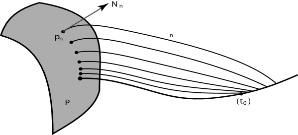
Figure 3. Bifurcation of geodesics starting orthogonally at a submanifold $P$, occurring at a $P$-focal point along $\gamma$.

The geodesic starting orthogonally at $P$ and terminating at the point $\gamma(s)$ are critical points of the geodesic action functional $F_{s}$ in (5.1) in the manifold $\Omega^{P}_{s}$ of all curves $x:[0,s]\to M$ of Sobolev class $H^{1}$ with $x(0)\in P$ and $x(s)=\gamma(s)$. For $x\in\Omega^{P}_{s}$, the tangent space $T_{x}\Omega_{s}^{P}$ is identified with the space of vector fields $V$ of class $H^{1}$ along $x$ such that $V(0)\in T_{x(0)}P$ and $V(s)=0$. For each $s\in\left]0,1\right]$, the second variation of $F_{s}$ at $\gamma|_{[0,s]}$ is given by the symmetric bounded bilinear form $I^{P}_{s}$ on $T_{\gamma}\Omega_{s}^{P}$ given by:

(6.2) $$I^{P}_{s}(V,W)=\int_{0}^{s}\Big{[}g(\tfrac{\mathrm{D}}{\mathrm{d}t}V,\tfrac{\mathrm{D}}{\mathrm{d}t}W)+g\big{(}R(\dot{\gamma},V)\,\dot{\gamma},W\big{)}\Big{]}\,\mathrm{d}\tau-S^{P}_{\dot{\gamma}(0)}\big{(}V(0),W(0)\big{)}.$$

Using a parallely transported orthonormal basis along $\gamma$, we will identify the tangent space $T_{\gamma}\Omega_{s}^{P}$ with the Hilbert space $H^{1}_{\mathfrak{P}}([0,s],I\!\!R^{n})$ of all maps $V:[0,s]\to I\!\!R^{n}$ of class $H^{1}$ such that $V(0)\in\mathfrak{P}$ and $V(s)=0$, where $\mathfrak{P}$ a subspace of $I\!\!R^{n}$ corresponding to $T_{\gamma(0)}P$ by the above identification of $T_{\gamma(0)}M$ with $I\!\!R^{n}$, and $\mathcal{S}$ is the bilinear form on $\mathfrak{P}$ corresponding to the second fundamental form $S^{P}_{\dot{\gamma}(0)}$. The space $H^{1}_{\mathfrak{P}}([0,1],I\!\!R^{n})$ will be endowed with the following Hilbert space inner product:

$$\langle V,W\rangle_{\mathfrak{P}}=\int_{0}^{s}g_{\scriptscriptstyle{\textrm{R}}}(V^{\prime},W^{\prime})\,\mathrm{d}t+g_{\scriptscriptstyle{\textrm{R}}}\big{(}V(0),W(0)\big{)}.$$

In order to reduce the focal bifurcation problem to a standard bifurcation setup, we need to modify slightly the construction done in Subsection 5.1; this is due to the fact that the map $\mathrm{EXP}$ as defined in (5.6), when evaluated on vector fields $V\in T_{\gamma}\Omega^{P}_{s}$, does not produce a curve starting on $P$. However, the reader will quickly convince himself that the exponential map $\exp_{\gamma(t)}$ in the definition of $\mathrm{EXP}$ in (5.6) can be equivalently replaced by the exponential map $\widetilde{\exp}_{\gamma(t)}$ of just about any other metric $\tilde{g}$ on (an open neighborhood of $\gamma$ in) $M$. Such replacement will not alter any of the results discussed insofar. In order to obtain a well defined map $\mathrm{EXP}$ that sends an open neighborhood of $0$ in $T_{\gamma}\Omega_{s}^{P}$ diffeomorphically onto an open neighborhood of $\gamma|_{[0,s]}$ in $\Omega_{s}^{P}$, it will then suffice to use the exponential map $\widetilde{\exp}$ of a (Riemannian) metric $\tilde{g}$ defined in an open subset $U\subset M$ containing $\gamma([0,1])$ with the property that $P$ is totally geodesic relatively to $\tilde{g}$ near $\gamma(0)$. Such a metric $\tilde{g}$ is easily found in a neighborhood of $\gamma(0)$ in $M$ using a submanifold chart for $P$ around $\gamma(0)$, and then extended using a partition of unity. Once this has been clarified, the reduction of the focal bifurcation problem to a standard bifurcation setup is done in perfect analogy with what discussed in Subsection 5.1: for all $s\in\left]0,1\right]$, an open neighborhood $\widetilde{\mathcal{W}}_{s}$ of $\gamma|_{[0,s]}$ in $\Omega^{P}_{s}$ is identified via $\mathrm{EXP}$ and a reparameterization map with a fixed open neighborhood $\mathcal{W}$ of $0$ in $H^{1}_{\mathfrak{P}}([0,1],I\!\!R^{n})$. This identification carries $\gamma|_{[0,s]}$ to $0$ for all $s$, and the family $(F_{s})$ of geodesic action functionals on $\widetilde{\mathcal{W}}_{s}$ to a smooth curve of functionals $f_{s}$ on $\mathcal{W}$. For all $s\in\left]0,1\right]$, the second variation of $f_{s}$ at $0$ is identified with a symmetric bilinear form $I^{P}_{s}$ on $H^{1}_{\mathfrak{P}}([0,1],I\!\!R^{n})$ given by:

(6.3) $$I^{P}_{s}(V,W)=\int_{0}^{1}\Big{[}\frac{1}{s}g\big{(}V^{\prime}(t),W^{\prime}(t)\big{)}+sg\big{(}R(st)V(t),W(t)\big{)}\Big{]}\,\mathrm{d}t-\mathcal{S}\big{(}V(0),W(0)\big{)}.$$

The smooth family of bilinear form $\hat{I}^{P}_{s}:=s\cdot I^{P}_{s}$, given by:

$$\hat{I}^{P}_{s}(V,W)=\int_{0}^{1}\Big{[}g\big{(}V^{\prime}(t),W^{\prime}(t)\big{)}+s^{2}g\big{(}R(st)V(t),W(t)\big{)}\Big{]}\,\mathrm{d}t-s\mathcal{S}\big{(}V(0),W(0)\big{)}$$

has a continuous extension to $s=0$.

Choose a maximal negative distribution $\Delta$ along $\gamma$ and define the space $\mathcal{S}^{\Delta}$ as in (4.9); the semi-Riemannian index theorem [10, Theorem 5.2] tells us that in this case, the $P$-Maslov index $\mathrm{i}_{\textrm{Maslov}}^{P}(\gamma)$ is given by:

(6.4) $$\mathrm{i}_{\textrm{Maslov}}^{P}(\gamma)=n_{-}\big{(}I^{P}_{1}|_{(\mathcal{S}^{\Delta})^{\perp_{I_{1}}}}\big{)}-n_{+}\big{(}I^{P}_{1}|_{\mathcal{S}^{\Delta}}\big{)}-n_{-}\big{(}g|_{T_{\gamma(0)}P}\big{)},$$

where $n_{-}\big{(}g|_{T_{\gamma(0)}P}\big{)}$ is the index of the restriction of $g$ to $T_{\gamma(0)}P$. Recall that this restriction is assumed nondegenerate, and, by continuity, $g$ will be also nondegenerate when restricted to tangent spaces of $P$ at points near $\gamma(0)$. In particular, the index $n_{-}\big{(}g|_{T_{q}P}\big{)}$ is constant for $q$ near $\gamma(0)$ in $P$.

Using Proposition 3.1 (recall formula (3.1)), from (6.4) we get that the spectral flow of the path $\hat{S}$ of Fredholm operators realizing the bilinear form $\hat{I}^{P}_{s}$ in $H^{1}_{\mathfrak{P}}([0,1],I\!\!R^{n})$ with respect to the inner product $\langle\cdot,\cdot\rangle_{\mathfrak{P}}$ is given by:

$$\mathrm{sf}(\hat{S})=-\mathrm{i}_{\textrm{Maslov}}^{P}(\gamma)-n_{-}\big{(}g|_{T_{\gamma(0)}P}\big{)}.$$

The above construction and arguments analogous to those used in the proofs of Corollary 5.5 and Corollary 5.6 give us the following conclusion:

Proposition 6.2.

Let $(M,g)$ be a semi-Riemannian manifold, $P\subset M$ a smooth submanifold and $\gamma:[0,1]\to M$ starting orthogonally on $P$; assume that $P$ is nondegenerate at $\gamma(0)$. Then, every non degenerate $P$-focal point with non zero signature is a bifurcation point relatively to the initial submanifold $P$. More generally, if $[a,b]\subset\left]0,1\right]$ is such that $\mathrm{i}_{\textrm{Maslov}}^{P}\big{(}\gamma|_{[0,a]}\big{)}\neq\mathrm{i}_{\textrm{Maslov}}^{P}\big{(}\gamma|_{[0,b]}\big{)}$, then there exists at least one bifurcation point relatively to the initial submanifold $P$ along $\gamma|_{\left]a,b\right[}$.

If $(M,g)$ is Riemannian, or if $(M,g)$ is Lorentzian and $\gamma$ is causal, then every $P$-focal point along $\gamma$ is a bifurcation point relatively to $P$.∎

6.2. Branching points along geodesics

A stronger property than bifurcation can be defined for a point $\gamma(t_{0})$ along a semi-Riemannian geodesic $\gamma$ by requiring the existence of a whole homotopy of geodesics $\gamma_{s}$, $s\in I$ where $I\subset I\!\!R$ is a right or a left neighborhood of $t_{0}$, such that $\gamma_{s}(a)=\gamma(a)$, $\gamma_{s}(s)=\gamma(s)$, $\gamma_{s}\neq\gamma$ and $\gamma_{s}\to\gamma$ as $s\to t_{0}$. This is for instance the case of the conjugate point along a meridian of the paraboloid mentioned in the Introduction. A point for which such stronger bifurcation property holds is called a branching point along $\gamma$. Using a classical Lyapunov-Schmidt reduction and the implicit function theorem, it is easy to prove that simple (i.e., multiplicity $1$) nondegenerate conjugate points along geodesics are branching points.

6.3. Bifurcation by geodesics with a fixed causal character

A different bifurcation problem in the context of semi-Riemannian geodesics may be formulated by requiring that the non trivial branch of geodesics have a fixed causal character. This is particularly interesting in the case of lightlike geodesics in Lorentzian manifolds, where light bifurcation may be used to model the so-called gravitational lensing problem in General Relativity. We observe here that the result of Corollary 5.6 does not apply to this situation.

6.4. Bifurcation at an isolated degenerate conjugate point

As we have observed ([6, 11]), degenerate conjugate points along a semi-Riemannian geodesic may accumulate; however, when the metric is real-analytic, an easy argument shows that conjugate points must necessarily be isolated. In the real-analytic case, the result of Corollary 5.5 can be generalized to the case of arbitrary conjugate points in terms of root functions and partial multiplicities, in the spirit of [12].

References

- [1] A. Abbondandolo, Morse Theory for Hamiltonian Systems, Pitman Research Notes in Mathematics, vol. 425, Chapman & Hall, London, 2001.
- [2] M. F. Atiyah, V. Patodi, I. M. Singer, Spectral Asymmetry and Riemannian Geometry III, Proc. Cambr. Phil. Soc. 79 (1976), 71–99.
- [3] P. M. Fitzpatrick, J. Pejsachowicz, L. Recht, Spectral Flow and Bifurcation of Strongly Indefinite Functionals Part I. General Theory, J. Funct. Anal. 162 (1) (1999), 52–95.
- [4] I. M. Gelfand, S. V. Fomin, Calculus of Variations, Prentic-Hall Inc., Englewood Cliffs, New Jersey, USA, 1963.
- [5] M. A. Krasnosel’skii, Topological Methods in the Theory of Nonlinear Integral Equations, Pergamon, Oxford, 1964.
- [6] F. Mercuri, P. Piccione, D. Tausk, Stability of the Conjugate Index, Degenerate Conjugate Points and the Maslov Index in semi-Riemannian Geometry, preprint 2001, to appear in the Pacific Journal of Mathematics.
- [7] P. Piccione, D. V. Tausk, An Index Theorem for Non Periodic Solutions of Hamiltonian Systems, Proceedings of the London Mathematical Society (3) 83 (2001), 351–389.
- [8] J. Phillips, Self-adjoint Fredholm Operators and Spectral Flow, Canad. Math. Bull. 39 (4) (1996), 460–467.
- [9] P. Piccione, D. V. Tausk, The Maslov Index and a Generalized Morse Index Theorem for Non Positive Definite Metrics, Comptes Rendus de l’Académie de Sciences de Paris, vol. 331, 5 (2000), 385–389.
- [10] P. Piccione, D. V. Tausk, The Morse Index Theorem in semi-Riemannian Geometry, Topology 41 (2002), no. 6, 1123–1159. (LANL math.DG/0011090).
- [11] P. Piccione, D. V. Tausk, On the Distribution of Conjugate Points along semi-Riemannian Geodesics, preprint 2000, to appear in Communications in Analysis and Geometry. (LANL math.DG/0011038)
- [12] P. J. Rabier, Generalized Jordan chains and two bifurcation theorems of Krasnosel’skii, Nonlinear Anal. 13 (1989), 903–934.