A Note on Shelling

Abstract.

The radial distribution function is a characteristic geometric quantity of a point set in Euclidean space that reflects itself in the corresponding diffraction spectrum and related objects of physical interest. The underlying combinatorial and algebraic structure is well understood for crystals, but less so for non-periodic arrangements such as mathematical quasicrystals or model sets. In this note, we summarise several aspects of central versus averaged shelling, illustrate the difference with explicit examples, and discuss the obstacles that emerge with aperiodic order.

1. Introduction

One characteristic geometric feature of a discrete point set $\varLambda\subset\mathbb{R}\hskip 0.5pt^{d}$, which might be thought of as the set of atomic positions of a solid, say, is the number of points of $\varLambda$ on shells of radius $r$ around an arbitrary, but fixed centre in $\mathbb{R}\hskip 0.5pt^{d}$. Of particular interest are special centres, such as points of $\varLambda$ itself, or other points that are fixed under non-trivial symmetries of $\varLambda$. This leads to the so-called shelling structure of $\varLambda$. Here, we consider infinite point sets only. In general, one obtains different answers for different centres, and one is then also interested in the average over all points of $\varLambda$ as centres, called the averaged shelling.

The spherical shelling of lattices and crystallographic point sets (i.e., periodic point sets whose periods span ambient space) is well studied, and many results are known in terms of generating functions. If $\varLambda$ is a lattice, the number of points on spheres of radius $r$ centre $0$ (central shelling) is usually encapsulated in terms of the lattice theta function [16, Ch. 2.2.3]

(1) $$\varTheta_{\varLambda}(z)\;=\;\sum_{x\in\varLambda}q^{x\cdot x}\;=\;\sum_{k}c(k)\,q^{k}$$

where $q=e^{\pi iz}$ and $c(k)$ is the number of lattice points of Euclidean square norm ($=$ square length) $k$. A closed expression for the latter can be given in many cases, see [16, Ch. 4] for details on root and weight lattices and various related packings, and [8] for an explicit example. There are many related lattice point problems, see [24] and references therein for recent developments.

One special feature of a lattice is that the shelling generating function is independent of the lattice point which is chosen as the centre – and, consequently, central and averaged shelling give the same result. Similarly, for uniformly discrete point sets that are crystallographic, the average is only over finitely many points in a fundamental domain and can often be calculated explicitly. For general uniformly discrete point sets, however, the situation is more complicated in that no two centres might give the same shelling function, or that the average may not be well defined. But there is one important class of point sets, the so-called model sets (also called cut-and-project sets, see [31, 4, 41, 43, 28, 14, 15] and references therein), which provide a high degree of order and coherence so that an extension of the shelling problem to these cases is possible, and has indeed been pursued. The original motivation for the investigation of model sets came from applications in physics. Meanwhile, due to interesting connections with several branches of mathematics, they are also studied in their own right, see [30, 37, 11] and [5] for details and further references. Below, we shall summarise the key properties of model sets needed for this article.

One of the earliest attempts to the shelling of model sets, to our knowledge, is that of Sadoc and Mosseri [40] who investigated the 4D Elser-Sloane quasicrystal [18] and then conjectured a formula for the central shelling of a close relative of it which was obtained by replacing the highly symmetric 4D polytype used in [18] by a 4D ball as a window. The conjecture was put right and proved in [33] by means of algebraic number theory revolving around the arithmetic of the icosian ring $\mathbb{I}$, a maximal order in the quaternion algebra $\mathbb{H}\hskip 0.5pt(\mathbb{Q}\hskip 0.5pt(\mbox{\small$\sqrt{5}\,$}))$. Recently, the central shelling was extended to the much more involved 3D case of icosahedral symmetry [46]. Also, some results exist on planar cases, e.g., for special eightfold and twelvefold symmetric cases with circular windows [34, 35].

The common aspect of all these extensions to model sets (or mathematical quasicrystals) is that only the central shelling of a highly symmetric representative has been considered, with a ball as window in internal space. This is a rather special situation which appears slightly artificial in view of the fact that the most relevant and best studied model sets usually have polytopes rather than balls as window, or, more generally, even compact sets with fractal boundary, cf. [4]. Also mathematically, the classical examples such as the rhombic Penrose or the Ammann-Beenker tiling are very attractive due to their rather intricate and unexpected topological nature [3, 19].

A more natural approach to model sets seems to be the averaged shelling, and it is the aim of this article to start to develop this idea. As we shall see, the topological structure will be manifest in the examples discussed below. On the other hand, the central shelling does have a universal meaning, too, if one considers it first for modules rather than for model sets. The window condition can then be imposed afterwards, see [8, 6, 7] for some examples. This approach is implicit in [33], but does not seem to have attracted much notice. It is important, though, because it leads to a separation of universal and non-universal aspects.

2. Central shelling

Many of the well studied planar tilings with non-crystallographic symmetries share the property that their vertices (or other typical point set representatives) form a discrete subset of rings of cyclotomic integers. This gives a nice and powerful link to results of algebraic number theory, which has, in fact, been used to construct model sets [38], and which also appeared before in a different context [29]. Let us thus first explain the situation of central shelling for these underlying dense point sets.

Let $\xi_{n}$ be a primitive $n$-th root of unity (with $n\geq 3$), e.g., $\xi_{n}=e^{2\pi i/n}$, and $\mathbb{Q}\hskip 0.5pt(\xi_{n})$ the corresponding cyclotomic field. Then, $\mathbb{Q}\hskip 0.5pt(\xi_{n}+\overline{\xi}_{n})$ is its maximal real subfield. From now on, we will use the following notation

(2) $$\mathbb{K}\hskip 0.5pt=\mathbb{Q}\hskip 0.5pt(\xi_{n})\,,\quad\Bbbk=\mathbb{Q}\hskip 0.5pt(\xi_{n}+\overline{\xi}_{n})\,,\quad\mathcal{O}=\mathbb{Z}[\xi_{n}]\,,\quad{\scriptstyle\mathcal{O}}=\mathbb{Z}[\xi_{n}+\overline{\xi}_{n}]\,,$$

where $\mathcal{O}$ is the ring of cyclotomic integers, which is the maximal order of $\mathbb{K}\hskip 0.5pt$, and ${\scriptstyle\mathcal{O}}$ is the ring of algebraic integers of $\Bbbk$, see [45].

Note that $\mathcal{O}$ is a $\mathbb{Z}$-module of rank $\varphi(n)$, where $\varphi$ denotes Euler’s totient function. The set $\mathcal{O}$, seen as a (generally dense) point set in $\mathbb{R}\hskip 0.5pt^{2}$, has $N$-fold rotational symmetry, where

(3) $$N\;=\;N(n)\;=\;\begin{cases}n&\text{if $n$ is even,}\\ 2n&\text{if $n$ is odd.}\end{cases}$$

This also means that $\mathcal{O}$ has precisely $N$ units on the unit circle, which are actually all roots of unity of $\mathbb{K}\hskip 0.5pt$. Also, $\mathbb{K}\hskip 0.5pt$ is a totally complex field extension of $\Bbbk$ of degree 2. It is known that, in this cyclotomic situation, the unique prime factorisation property of $\mathcal{O}$ (i.e., class number one) implies that of ${\scriptstyle\mathcal{O}}$, and this happens in precisely 29 cases, compare [45, Thm. 11.1], namely for

(4) $$\begin{split}n\in\{&3,4,5,7,8,9,11,12,13,15,16,17,19,20,21,\\ &24,25,27,28,32,33,35,36,40,44,45,48,60,84\}\,,\end{split}$$

where $n\not\equiv 2\bmod 4$ to avoid double counting. Note that $n=1$ ($N=2$) is excluded here because it corresponds to $\mathbb{K}\hskip 0.5pt=\mathbb{Q}\hskip 0.5pt$ with $\mathcal{O}=\mathbb{Z}$, which is only one-dimensional.

Now, let $p$ be a prime of ${\scriptstyle\mathcal{O}}$. Then, in going from ${\scriptstyle\mathcal{O}}$ to $\mathcal{O}$, precisely one of the following cases applies, see [36, Ch. I] and [45, Ch. 4]:

• $p$ ramifies, i.e., $p=P\overline{P}$ with $P$ a prime and $\overline{P}/P$ a root of unity in $\mathcal{O}$.

• $p$ is inert, i.e., $p$ is also prime in $\mathcal{O}$.

• $p$ is a splitting prime of $\mathcal{O}/{\scriptstyle\mathcal{O}}$, i.e., $p=P\overline{P}$ with $\overline{P}/P$ not a unit in $\mathcal{O}$.

Up to units, all primes of $\mathcal{O}$ appear this way.

Prime factorisation in ${\scriptstyle\mathcal{O}}$ versus $\mathcal{O}$ can now be employed to find the combinatorial structure of the shells. We encode this into the central shelling function $c(r^{2})$ which counts the number of points on shells (circles) of radius $r$. By convention, $c(0)=1$.

Theorem 1.

Let $\mathcal{O}=\mathbb{Z}[\xi_{n}]$ be any of the $29$ planar $\mathbb{Z}$-modules that consist of the integers of a cyclotomic field with class number one. Then, for $r^{2}>0$, the function $c(r^{2})$ vanishes unless $r^{2}\in{\scriptstyle\mathcal{O}}$ and all inert prime factors of $r^{2}$ occur with even powers only. In this case,

(5) $$c(r^{2})\;=\;N\cdot\!\!\prod_{\stackrel{{\scriptstyle\scriptstyle p\mid r^{2}}}{{\scriptstyle p\;{\rm splits}}}}\!\!\big{(}t(p)+1\big{)}\,,$$

where $p$ runs through a representative set of the primes of ${\scriptstyle\mathcal{O}}$. Here, $t(p)$ is the maximal power $t$ such that $p^{t}$ divides $r^{2}$. The prefactor, $N=N(n)$ of Eq. $(\ref{symm})$, reflects the point symmetry of the module. Furthermore, $r^{2}$ is then a totally positive number in ${\scriptstyle\mathcal{O}}$, i.e., all its algebraic conjugates are positive as well.

Proof.

Since $c(0)=1$ by convention, consider $r^{2}>0$. If there exists a number $x\in\mathcal{O}$ on the shell of radius $r$ around $0$, we must have $r^{2}=x\overline{x}$, hence $r^{2}\in{\scriptstyle\mathcal{O}}$. In this case, any inert prime factor $p$ of $r^{2}$ (in ${\scriptstyle\mathcal{O}}$) necessarily divides both $x$ and $\overline{x}$ (in $\mathcal{O}$). Consequently, the maximal power $t=t(p)$ such that $p^{t}$ divides $r^{2}$ must be even.

Conversely, assume $r^{2}>0$ and $t(p)$ even for all inert primes of ${\scriptstyle\mathcal{O}}$. If a ramified or a splitting prime $p=P\overline{P}$ divides $r^{2}$, we know that equal powers of $P$ and $\overline{P}$ occur in the prime factorisation of $r^{2}$ in $\mathcal{O}$. Consequently, we can group the prime factors of $r^{2}$ in $\mathcal{O}$ into two complex conjugate numbers, i.e., we have at least one solution of the equation $r^{2}=x\overline{x}$ with $x\in\mathcal{O}$, so $c(r^{2})>0$.

Consider a non-empty shell with $r^{2}>0$, i.e., $r^{2}=x\overline{x}$ for some $0\neq x\in\mathcal{O}$. Consider the prime factorisation $r^{2}=e\cdot p_{1}^{t_{1}}\cdot\ldots\cdot p_{s}^{t_{s}}$ in ${\scriptstyle\mathcal{O}}$, with $e$ a unit. If $p_{i}$ is not a splitting prime, the distribution of the corresponding primes in $\mathcal{O}$ to $x$ and $\overline{x}$ is unique, up to units of $\mathcal{O}$.

If, however, $p_{j}=P_{j}\overline{P}_{j}$ is a splitting prime, we have to distribute $(P_{j}\overline{P}_{j})^{t_{j}}$ over $x$ and $\overline{x}$. In view of $\overline{P}_{j}$ being the complex conjugate of $P_{j}$, but not an algebraic conjugate, we have the options of $(P_{j})^{s}(\overline{P}_{j})^{t_{j}-s}$ as factor of $x$ and $(\overline{P}_{j})^{s}(P_{j})^{t_{j}-s}$ as factor of $\overline{x}$, for any $0\leq s\leq t_{j}$. This amounts to $t_{j}+1$ different possibilities, which gives the corresponding factor in (5).

As mentioned above, there are $N$ units of $\mathcal{O}$ on the unit circle. This means that, as soon as $r^{2}>0$, points on the shells come in sets of $N$, which gives the prefactor in (5). Together with the previous arguments, this explains the multiplicative structure of $c/N$.

Finally, assume $r^{2}=x\overline{x}$ for some $0\neq x\in\mathcal{O}$ and let $\sigma$ be any Galois automorphism of $\mathbb{K}\hskip 0.5pt$ over $\mathbb{Q}\hskip 0.5pt$. Then we have

$$0\;<\;\sigma(x)\overline{\sigma(x)}\;=\;\sigma(x)\sigma(\overline{x})\;=\;\sigma(x\overline{x})\;=\;\sigma(r^{2})$$

so also all algebraic conjugates of $r^{2}$ are positive. This shows that $r^{2}$ is totally positive. ∎

Remark: It is clear that Theorem 1 can be generalised to the situation that $\mathbb{K}\hskip 0.5pt$ is a totally complex field extension of a totally real field $\Bbbk$ whenever $\mathbb{K}\hskip 0.5pt$ has class number one, with sets of integers $\mathcal{O}$ and ${\scriptstyle\mathcal{O}}$ as above, compare [45, Thm. 4.10]. In this case, the prefactor in Eq. (5) has to be replaced by the number of elements in the unit group of $\mathcal{O}$ that lie on the unit circle.

Let us consider the cyclotomic case in more detail. If $V(r^{2})=\{x\in\mathcal{O}\mid x\overline{x}=r^{2}\}$, and $\sigma$ is any Galois automorphism of $\mathbb{K}\hskip 0.5pt/\mathbb{Q}\hskip 0.5pt$, then $\sigma(\mathcal{O})=\mathcal{O}$ and $V(r^{2})$ is mapped bijectively to $V(\sigma(r^{2}))$. This means that $c(r^{2})=c(\sigma(r^{2}))$.

Moreover, consider the situation that two totally positive numbers of ${\scriptstyle\mathcal{O}}$, $r^{2}$ and $R^{2}$, are related by $R^{2}=er^{2}$, with $e$ a unit in ${\scriptstyle\mathcal{O}}$. Clearly, $e$ is then also totally positive. If $e$ is of the form $e=u\overline{u}$, with $u$ a unit in $\mathcal{O}$, the mapping $x\mapsto ux$ gives a bijection between $V(r^{2})$ and $V(R^{2})$, hence $c(r^{2})=c(R^{2})$. If all totally positive units of ${\scriptstyle\mathcal{O}}$ are of this form, which includes the case that $e$ is the square of a unit in $\mathcal{O}$, we may conclude that the central shelling function $c$ only depends on the principal ideal of ${\scriptstyle\mathcal{O}}$ generated by $r^{2}$.

In general cyclotomic fields, this factorisation property of totally positive units need not be satisfied (e.g., it fails for $n=29$). However, it is true for all class number one cases. More precisely, if $n$ is a power of $2$, all totally positive units of ${\scriptstyle\mathcal{O}}$ are squares of units of $\mathcal{O}$, which is known as Weber’s theorem, compare [21, Cor. 1 and Rem. 2]. The same statement holds if $n$ is an odd prime below 100, except for $n=29$, see [21, Ex. 2]. We checked explicitly, using the KANT program package [17, 26], that this remains true for all $n$ from our list (4) that are prime powers. All remaining cases of (4) are composite integers. Here, not all totally positive units of ${\scriptstyle\mathcal{O}}$ are squares in $\mathcal{O}$, but they are of the form $e=u\overline{u}$, with $u$ a unit in $\mathcal{O}$. This was again checked using KANT. The difference to the other cases comes from the additional unit $u=1-\xi_{n}$, compare [45, Cor. 4.13].

We may conclude as follows.

Fact 1.

Let $\mathcal{O}=\mathbb{Z}[\xi_{n}]$ be any of the $29$ planar $\mathbb{Z}$-modules that consist of the integers of a cyclotomic field with class number one, and ${\scriptstyle\mathcal{O}}=\mathbb{Z}[\xi_{n}+\overline{\xi}_{n}]$. Then, the central shelling function $c$ for $\mathcal{O}$ depends on $r^{2}\in{\scriptstyle\mathcal{O}}$ only via the principal ideal $r^{2}{\scriptstyle\mathcal{O}}$ generated by it. ∎

This allows us to reformulate the result of Theorem 1 by means of ideals and characters of the field extension $\mathbb{K}\hskip 0.5pt/\Bbbk$. By a character $\chi\not\equiv 0$, we here mean a totally multiplicative real function of the ideals of ${\scriptstyle\mathcal{O}}$, i.e., $\chi(\mathfrak{ab})=\chi(\mathfrak{a})\chi(\mathfrak{b})$ for all ideals $\mathfrak{a}$ and $\mathfrak{b}$ of ${\scriptstyle\mathcal{O}}$, see [36, Ch. VII.6] for background material. In particular, $\chi({\scriptstyle\mathcal{O}})=1$. It suffices to specify the values of $\chi$ for all prime ideals $\mathfrak{p}$ of ${\scriptstyle\mathcal{O}}$. We define

(6) $$\chi(\mathfrak{p})\;=\;\begin{cases}\hphantom{-}0&\text{if $\mathfrak{p}$ ramifies}\\ -1&\text{if $\mathfrak{p}$ is inert}\\ \hphantom{-}1&\text{if $\mathfrak{p}$ splits}\end{cases}$$

where the property of the prime ideal $\mathfrak{p}$ refers to the behaviour under the field extension from $\Bbbk$ to $\mathbb{K}\hskip 0.5pt$. This leads to the following result.

Corollary 1.

Under the assumptions of Theorem 1, the central shelling function $c$ is proportional to the summatory function of the character $\chi$ of Eq. $(\ref{chardef})$, i.e.,

(7) $$c(r^{2}{\scriptstyle\mathcal{O}})\;=\;N\cdot\sum_{\mathfrak{a}\mid(r^{2}{\scriptscriptstyle\mathcal{O}})}\chi(\mathfrak{a}),$$

with $N$ given by Eq. $(\ref{symm})$.

Proof.

Due to unique prime factorisation in ${\scriptstyle\mathcal{O}}$ and the multiplicative structure of $c/N$ according to Eq. (5), it is sufficient to verify the claim for prime powers, i.e., for $r^{2}{\scriptstyle\mathcal{O}}=\mathfrak{p}^{\ell}$. Clearly, if $\mathfrak{p}$ ramifies, the sum in Eq. (7) gives $c(\mathfrak{p}^{\ell})=1$ for all $\ell\geq 0$. The alternating sign of $\chi(\mathfrak{p}^{\ell})$ for inert $\mathfrak{p}$ implies $c(\mathfrak{p}^{\ell})=0$ for odd $\ell$ and $c(\mathfrak{p}^{\ell})=1$ otherwise. If $\mathfrak{p}$ splits, the right hand side of Eq. (7) adds up to $\ell+1$. Invoking Fact 1 and a comparison with Eq. (5) completes the proof. ∎

The explicit use of Theorem 1 and Corollary 1 requires the knowledge of the splitting structure of the primes. Examples can be found in [39, 6, 7], see also [34, 35]. If one is interested in the central shelling of a model set rather than that of the underlying (dense) module, one has to take the window into account as a second step. A model set $\varLambda(\varOmega)$ in “physical space” $\mathbb{R}\hskip 0.5pt^{d}$ is defined within the following cut-and-project scheme [31, 4]

(8) $$\begin{array}[]{ccccc}\mathbb{R}\hskip 0.5pt^{d}&\xleftarrow[\qquad]{\pi}&\mathbb{R}\hskip 0.5pt^{d}\times H&\xrightarrow[\qquad]{\pi_{H}}&H\\ \cup&&\cup&&\cup\makebox[0.0pt][l]{\small\ \ dense}\\ L&\xleftarrow[\qquad]{1-1}&\varGamma&\xrightarrow[\qquad]{}&L^{*}\\ \end{array}$$

where the “internal space” $H$ is a locally compact Abelian group, and $\varGamma\subset\mathbb{R}\hskip 0.5pt^{d}\times H$ is a lattice, i.e., a co-compact discrete subgroup. The projection $L^{*}=\pi_{H}(\varGamma)$ is assumed to be dense in internal space, and the projection into physical space has to be one-to-one on $\varGamma$. Consequently, the mapping ${\,}^{*}$: $L\longrightarrow L^{*}\subset H$, with ${\,}^{*}=\pi_{H}\circ\big{(}\pi|_{\varGamma}\big{)}^{-1}$, is well defined. It is called the $*$-map of the cut-and-project formalism, compare [31]. Note that the $*$-map need not be injective, i.e., its kernel can be a nontrivial subgroup of $L$.

A model set $\varLambda(\varOmega)$ is now defined as

(9) $$\varLambda(\varOmega)\;=\;\left\{x\in L\mid x^{*}\in\varOmega\right\}\;=\;\left\{\pi(y)\mid y\in\varGamma,\,\pi_{H}(y)\in\varOmega\right\}\;\subset\;\mathbb{R}\hskip 0.5pt^{d},$$

where the window $\varOmega\subset H$ is a relatively compact set with non-empty interior. Usually, one either takes an open set or a compact set that is the closure of its interior. Note that the $*$-map is well defined on $\varLambda(\varOmega)$, with $\big{(}\varLambda(\varOmega)\big{)}^{*}\subset\varOmega$. More generally, also sets of the form $t+\varLambda(\varOmega)$ with $t\in\mathbb{R}\hskip 0.5pt^{d}$ are called model sets. If $t\in L$, one has $t+\varLambda(\varOmega)=\varLambda(t^{*}+\varOmega)$ and is back to the case of Eq. (9), which is sufficient for our discussion. For the above example of a cyclotomic field $\mathbb{K}\hskip 0.5pt=\mathbb{Q}\hskip 0.5pt(\xi_{n})$, we need $d=\varphi(n)$ to construct model sets with $n$-fold symmetry, compare [10, App. A].

In order to compute the central shelling for a model set $\varLambda(\varOmega)$, one first determines all points of the module $L=\pi(\varGamma)$ on the shell of a given radius $r$. Then, the window $\varOmega$ decides, according to the filtering process of Eq. (9), which of these points actually appear in the model set, and the shelling formula is modified accordingly. As long as we are dealing with a one-component model set (i.e., as long as all points are in one translation class), the formula of Theorem 1 thus gives an upper bound on the shelling number in the model set. As mentioned above, the central shelling of a few model sets with spherical windows [40, 33, 34, 35, 46] has been considered in detail.

3. Averaged shelling

A moment’s reflection reveals that the averaged shelling is considerably more involved. In order to determine the averages, one would need to know all possible local configurations up to a given diameter together with their frequencies, provided the latter are well defined. In general, this is not the case, as cluster or patch frequencies in general Delone sets need not exist. However, regular model sets are particularly nice in this respect because all patch frequencies exist uniformly [41], which is equivalent to unique ergodicity of the corresponding dynamical system [44, 42] (under the translation action of $\mathbb{R}\hskip 0.5pt^{d}$). Moreover, due to existence of the cut-and-project scheme (8) and Weyl’s theorem, compare [32], it is possible to transfer the averaging part of the combinatorial problem to one of analysis.

Let us also point out that Eq. (1) for a model set does not make much sense as it would depend on the representative chosen, rather than being a quantity attached to an entire local indistinguishability (LI) class, compare [43, 4]. If $\varLambda$ is a lattice, $\varLambda-\varLambda=\varLambda$, and we could equally well sum over the difference set in (1). Using this for model sets would give $\sum_{x\in\varLambda-\varLambda}q^{x\cdot x}$ which is constant on the LI class. However, this still does not reflect the statistical aspects of the (local) shells, because each $x\in\varLambda-\varLambda$ is counted with weight one. Let us thus introduce the averaged shelling function $a(r^{2})$ as the number of points on a shell of radius $r$, averaged over all points of $\varLambda$ as possible centres of the shells.

Now, let $\varLambda=\varLambda(\varOmega)$ be a regular, generic model set, in the terminology of [31], with window $\varOmega$, i.e., $\varOmega$ is a relatively compact set in $H$ with non-empty interior, boundary of measure $0$, and $\partial\varOmega\cap\pi_{H}(\varGamma)=\varnothing$. For simplicity, we also assume that $H=\mathbb{R}\hskip 0.5pt^{m}$, though a generalisation of what we say below to the case of general locally compact Abelian groups is possible. In analogy to Eq. (1), a generalised theta series could be defined ad hoc as

(10) $$\varTheta_{\varLambda}(z)\;:=\;\sum_{r\in\mathcal{R}}a(r^{2})\,q^{r^{2}}$$

where $q=e^{\pi iz}$ and $\mathcal{R}=\{r\in\mathbb{R}\hskip 0.5pt_{\geq 0}\mid|y|=r\mbox{ for some }y\in\varLambda-\varLambda\}$ is the set of possible radii as obtained from the set of difference vectors between points of $\varLambda$. The coefficient $a(r^{2})$ is now meant as the averaged quantity defined above, which we will now calculate.

Let $\nu(y)$ denote the relative frequency of the difference $y$ between two points of the model set (hence $y\in\varLambda-\varLambda$). Up to the overall density of the model set, $\nu(y)$ is an autocorrelation coefficient of the point set $\varLambda$. This quantity exists uniformly for all $y$ as a consequence of the model set structure [23, 41, 32]. But then, we obviously obtain

(11) $$a(r^{2})\;=\;\sum_{\stackrel{{\scriptstyle\scriptstyle y\in\varLambda-\varLambda}}{{\scriptstyle|y|=r}}}\,\nu(y)\,.$$

On the other hand, if $\varLambda_{s}=\{x\in\varLambda\mid|x|<s\}$, one has

(12) $$\nu(y) = \lim_{s\to\infty}\frac{1}{|\varLambda_{s}|}\sum_{\stackrel{{\scriptstyle\scriptstyle x\in\varLambda_{s}}}{{\scriptstyle x+y\in\varLambda}}}1\;\,=\;\,\lim_{s\to\infty}\frac{1}{|(\varLambda_{s})^{*}|}\sum_{\stackrel{{\scriptstyle\scriptstyle x^{*}\in(\varLambda_{s})^{*}}}{{\scriptstyle(x+y)^{*}\in\varOmega}}}1$$

$$= \frac{1}{{\rm vol}(\varOmega)}\int_{\mathbb{R}\hskip 0.5pt^{m}}\boldsymbol{1}_{\varOmega}(z)\,\boldsymbol{1}_{\varOmega}(z+y^{*})\,{\rm d}z$$

where $\boldsymbol{1}_{\varOmega}$ is the characteristic function of the window. Note that, as the $*$-map need not be injective, the second equality may only hold in the limit $s\to\infty$ (this step is implicit in the proof of [41, Thm. 1]). We add it here because it shows how the counting is transfered to internal space, in particular in the cases where the $*$-map is one-to-one, which is the situation we will meet in the examples.

The last step in (12) is now a direct application of Weyl’s theorem on uniform distribution. This is justified here because $(\varLambda_{s})^{*}$, for increasing $s$, gives a sequence of points in $\varOmega$ that are uniformly distributed, see [23, 32] and [41, Thm. 1], and because $\partial\varOmega$ has measure $0$ by assumption. In this situation, the averaged quantities are the same for generic and singular members of the LI class [41, 4]. Moreover, it also does not change if $\,\partial\varOmega\cap L^{*}\neq\varnothing$, so that the corresponding assumption can be dropped. Consequently, the averaged shelling function is constant on LI classes of regular model sets. We combine Eqs. (11) and (12) to obtain

Theorem 2.

Let $\varLambda$ be a regular model set in the sense of Moody [31], obtained from a cut-and-project scheme $(\ref{candp})$ with internal space $H=\mathbb{R}\hskip 0.5pt^{m}$ and window $\varOmega$. Then, the averaged shelling function $a(r^{2})$ exists, and is given by

(13) $$a(r^{2})\;=\;\frac{1}{{\rm vol}(\varOmega)}\sum_{\stackrel{{\scriptstyle\scriptstyle y\in\varLambda-\varLambda}}{{\scriptstyle|y|=r}}}{\rm vol}\big{(}\varOmega\cap(\varOmega-y^{*})\big{)}.$$

In particular, $a(r^{2})$ vanishes if there is no $y\in\varLambda-\varLambda$ with $y\cdot y=r^{2}$.∎

Remark: This result allows the calculation of the shelling function, for any possible radius $r$, by evaluating finitely many volumes in internal space. This is so because a model set $\varLambda$ has the additional property that also its difference set, $\varLambda-\varLambda$, is uniformly discrete, so that there are only finitely many different solutions of $|y|=r$ with $y\in\varLambda-\varLambda$.

4. Examples

Let us first consider a well-known model set in one dimension, the Fibonacci chain, which can be described as

(14) $$\varLambda_{\text{F}}\;=\;\big{\{}x\in\mathbb{Z}[\tau]\mid x^{*}\in[-1,\tau-1]\,\big{\}}\;=\;\varLambda\big{(}[-1,\tau-1]\big{)},$$

where $\mathbb{Z}[\tau]=\{m+n\tau\mid m,n\in\mathbb{Z}\}$ is the ring of integers in the quadratic field $\mathbb{Q}\hskip 0.5pt(\tau)$ and $\tau=(1+\sqrt{5}\,)/2$ is the golden ratio. The $*$-map in this setting is algebraic conjugation in $\mathbb{Q}\hskip 0.5pt(\tau)$, defined by $\sqrt{5}\mapsto-\sqrt{5}$. The 2D lattice behind this formulation is $\varGamma=\{(x,x^{*})\mid x\in\mathbb{Z}[\tau]\}$. A short calculation results in $\varLambda_{\text{F}}-\varLambda_{\text{F}}=\varLambda\big{(}[-\tau,\tau]\big{)}$, and

(15) $$\nu(y)\;=\;\nu(-y)\;=\;f_{\text{F}}(y^{*})\;=\;\begin{cases}0&\text{if $|y^{*}|>\tau$}\\ 1-|y^{*}|/\tau&\text{if $|y^{*}|\leq\tau$}\end{cases}$$

so that the averaged shelling function for the Fibonacci chain (and thus also for its entire LI class) is $a(0)=1$ and $a(r^{2})=2f_{\text{F}}(y^{*})$ for any non-zero distance $r$ that is the absolute value of a number $y\in\varLambda_{\text{F}}-\varLambda_{\text{F}}\subset\mathbb{Z}[\tau]$. Also, all shelling numbers $a(r^{2})$ are elements of $\mathbb{Z}[\tau]$, as can easily be seen from formula (15). This has a topological interpretation, as we will briefly explain below for a more significant example.

In internal space, the function $f_{\text{F}}$ has a piecewise linear continuation, but the function $a(r^{2})$ looks rather erratic, compare [8] for a similar example. This is a consequence of the properties of the $*$-map, being algebraic conjugation in this case. As a mapping, it is totally discontinuous on $L^{*}$ (and also on its rational span) when the latter is given the induced topology of the ambient space $H$. In a different topology, however, this map becomes uniformly continuous, and it is this alternative setting, compare [12], which explains the appearance of the internal space from intrinsic data of a model set $\varLambda$.

Figure 1. Radial component of the frequency functions $f_{m}(s)$ of Eqs. (16), (19) and (20) for dimensions $m=1,2,3,5,10,50$ of internal space.

As another example, let us once more look at the circular shelling in the plane, i.e., at a 2D model set with an open disk (radius $R$, centre $0$) as window in 2D internal space. So, $\varOmega=B_{R}(0)$ and, consequently, $\varOmega-\varOmega=B_{2R}(0)$. We have $\nu(y)=f_{2}(y^{*})$, where, due to rotational symmetry of the window, the function $f_{2}$ only depends on $s=|y^{*}|$. Explicitly, it is given by

(16) $$f_{2}(s)\;=\;\frac{{\rm vol}\big{(}B_{R}(0)\cap B_{R}(s)\big{)}}{{\rm vol}\big{(}B_{R}(0)\big{)}}\;=\;\frac{2}{\pi}\,\arccos\left(\frac{s}{2R}\right)\;-\;\frac{s}{\pi R}\sqrt{1-\left(\frac{s}{2R}\right)^{2}}$$

for $0\leq s<2R$ and $f_{2}(s)=0$ otherwise. Fig. 1 contains a graph of $f_{2}(s)$. This function, often called the covariogram of the disk, is a radially symmetric positive definite function known as Euclid’s hat, see [22, p. 100].

To calculate $a(r^{2})$, one has to sum finitely many terms of this kind, according to Eq. (11). This situation of a 2D internal space shows up for planar model sets with $n\in\{5,8,12\}$, because these are the cases with $\varphi(n)=4$. Here, one simply obtains

(17) $$a(r^{2})\;=\;c(r^{2})\,f_{2}(s)$$

where $c(r^{2})$ is the central shelling function of Eq. (5) and $s=|y^{*}|$ for any $y$ on the shell of radius $r$. This is so because the window is a disk and the $*$-map sends all cyclotomic integers on a circle to a single circle in internal space. Consequently, the central shelling provides an upper bound for the average shelling in this case.

Part of this result can be extended to arbitrary dimension. For two intersecting $m$-dimensional balls of radius $R$, the overlap consists of two congruent ball segments. The corresponding volume can be calculated by integrating slices (which are balls of dimension $m-1$). Dividing by the volume of the $m$-ball, the covariogram becomes

(18) $$f_{m}(s)\;=\;\frac{2\,\Gamma(\frac{m}{2}+1)}{\sqrt{\pi}\,\Gamma(\frac{m+1}{2})}\int\limits_{0}^{\arccos(\frac{s}{2R})}\sin^{m}(\alpha)\,{\rm d}\alpha.$$

The integral can be expanded in terms of Chebyshev polynomials. For even $m=2\ell$, this yields

(19) $$\begin{split}f_{2\ell}(s)\;=\;{}&\frac{\Gamma(\ell+1)}{2^{2\ell-1}\sqrt{\pi}\,\Gamma(\ell+\tfrac{1}{2})}\Bigg{[}\binom{2\ell}{\ell}\,\arccos\left(\frac{s}{2R}\right)\\[2.84526pt] &+\;\sqrt{1-\left(\frac{s}{2R}\right)^{2}}\,\sum\limits_{k=1}^{\ell}\frac{(-1)^{k}}{k}\,\binom{2\ell}{\ell-k}\,U_{2k-1}\left(\frac{s}{2R}\right)\Bigg{]}\end{split}$$

where $U_{k}(x)=\sin\big{(}(k+1)\arccos(x)\big{)}/\sin\big{(}\arccos(x)\big{)}$ are the Chebyshev polynomials of the second kind [1, Ch. 22]. For odd dimension, $m=2\ell+1$, one obtains the following expression

(20) $$f_{2\ell+1}(s)\;=\;1-\frac{\Gamma(\ell+\tfrac{3}{2})}{2^{2\ell-1}\sqrt{\pi}\,\Gamma(\ell+1)}\,\sum\limits_{k=0}^{\ell}\frac{(-1)^{k}}{2k+1}\,\binom{2\ell+1}{\ell-k}\,T_{2k+1}\left(\frac{s}{2R}\right)$$

in terms of the Chebyshev polynomials $T_{k}(x)=\cos\big{(}k\arccos(x)\big{)}$ of the first kind [1, Ch. 22]. Eqs. (18)–(20) are valid for $0\leq s<2R$; for distances larger than the diameter, the overlap vanishes, hence $f_{m}(s)=0$ for $s\geq 2R$. Eq. (16) is recovered from (19) for $\ell=1$. The functions $f_{m}(s)$ for various dimensions $m$ are shown in Fig. 1. Unfortunately, for $m>2$, there is no simple generalisation of Eq. (17), because the $*$-map is then more complicated.

Let us finally consider an eightfold symmetric model set in the plane, based on the classical Ammann-Beenker or octagonal tiling, compare [2, 8, 9] and references therein. It is usually described by projection from four dimensions, where we use the lattice $\varGamma=\sqrt{2}\,\mathbb{Z}^{4}$. The projections $\pi$ and $\pi_{H}$ of (8) are essentially determined by compatibility with eightfold symmetry. In a convenient coordinatisation [9], the images $\boldsymbol{a}_{j}$, $j\in\{1,2,3,4\}$, of the standard basis vectors of the lattice have unit length in physical space, and the same is true of the corresponding projections $\boldsymbol{a}_{j}^{*}$ in internal space. Observing that $\mathbb{Z}\boldsymbol{a}_{1}+\mathbb{Z}\boldsymbol{a}_{2}+\mathbb{Z}\boldsymbol{a}_{3}+\mathbb{Z}\boldsymbol{a}_{4}=\mathbb{Z}[\xi_{8}]$, we can continue with a formulation based on the cyclotomic integers, compare [38]. For the Ammann-Beenker tiling, the window is then a regular octagon $O$ of unit edge length, see Fig. 2. Note that the window is invariant under the symmetry group $D_{8}$ of order $16$.

       

Figure 2. A patch of the Ammann-Beenker tiling with vertex set $\varLambda_{\rm AB}$ (left) and the $*$-image of $\varLambda_{\rm AB}$ inside the octagonal window in internal space (right), with relative scale as described in the text.

Explicitly, the corresponding point set in the plane is given by

(21) $$\varLambda_{\text{AB}}\;=\;\big{\{}z\in\mathbb{Z}[\xi_{8}]\mid z^{*}\in O\big{\}},$$

where ${\,}^{*}$ is the Galois automorphism defined by $\xi_{8}\mapsto\xi_{8}^{3}$. If we choose $\xi_{8}=\xi=e^{2\pi i/8}$ and identify $\mathbb{R}\hskip 0.5pt^{2}$ with $\mathbb{C}\hskip 0.5pt$, this gives $\boldsymbol{a}_{j}=\xi^{j-1}$, $1\leq j\leq 4$, while the $*$-images satisfy $\boldsymbol{a}_{j}^{*}=\xi^{3(j-1)}$, compare Fig. 3.

Figure 3. Vectors $\boldsymbol{a}_{j}$ in physical and $\boldsymbol{a}_{j}^{*}$ in internal space related by the $*$-map.

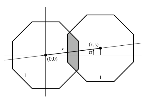
Figure 4. Two overlapping regular octagons at distance $s$.

A somewhat tedious, but elementary calculation on the basis of Fig. 4 gives

Fact 2.

The covariogram of the regular octagon of edge length one is

(22) $$f_{\rm AB}(s,\alpha)\;=\;\begin{cases}0&\mbox{if\/ $\lambda\leq x$}\\ \frac{(\lambda-2)(x+y)x}{2}+\frac{\lambda(1-x)}{2}+\frac{(1-y)}{2}\quad&\mbox{if\/ $\lambda-y\leq x\leq\lambda$}\\ \frac{(\lambda-2)(x^{2}-y^{2})}{4}-\frac{(\lambda-1)x}{2}+\frac{\lambda+2}{4}\quad&\mbox{if\/ $1+y\leq x\leq\lambda-y$}\\ \frac{(\lambda-2)(x-y-1)y}{2}-\frac{x}{2}+1&\mbox{if\/ $0\leq x\leq 1+y$}\end{cases}$$

where $\lambda=1+\sqrt{2}$,

$$x\;=\;s\,\cos\alpha^{\prime}\;\in\;\Big{[}{\textstyle\frac{s}{2}\sqrt{2+\sqrt{2}}},s\Big{]}\,,\qquad y\;=\;s\,\sin\alpha^{\prime}\;\in\;\Big{[}0,{\textstyle\frac{s}{2}\sqrt{2-\sqrt{2}}}\,\Big{]}\,,$$

and where $\alpha^{\prime}$ is the unique angle in the interval $[0,\frac{\pi}{8}]$ that is related to $\alpha$ by the $D_{8}$ symmetry of the octagon. ∎

A contour map of $f_{\text{AB}}(s,\alpha)$ is shown in Fig. 5. It demonstrates that the previous consideration of a circular window is actually a reasonable approximation to this case. It is sufficient for most applications concerning (powder) diffraction, compare [25, Ch. 3].

Figure 5. Contour map of the function $f_{\text{AB}}(s,\alpha)$ of (22) in internal space. The contours show the decrease of $f_{\text{AB}}$ from its maximum value $f_{\text{AB}}(0,0)=1$ to $f_{\text{AB}}(s,\alpha)=0$ outside the outer octagonal contour.

We can now calculate the averaged shelling coefficient $a(r^{2})$ of (11) explicitly for any distance $r$ in $\varLambda_{\rm AB}$. The results for all distances with $0<r^{2}\leq 5$ are summarised in Table 1. They confirm the results of [8] which had been obtained numerically.

As an explicit example, let us consider the shortest distance in the model set. This is $r=\sqrt{2-\sqrt{2}}=2\sin(\frac{\pi}{8})$ which is realised by the short diagonal of the rhomb. In this case, there are eight numbers $z\in\varLambda_{\text{AB}}-\varLambda_{\text{AB}}$ that contribute to Eq. (11). They form a single $D_{8}$ orbit; one representative is listed in Table 1. Due to the symmetry of the window, the contribution of each member of the orbit is the same, so it suffices to consider a representative and to multiply the result by the corresponding orbit length. Choosing $z=1-\xi$, we find $z^{*}=1-\xi^{3}$, hence $|z^{*}|=\sqrt{2+\sqrt{2}}=2\cos(\frac{\pi}{8})$; the corresponding angle is $\alpha=-\frac{\pi}{8}$, hence $\alpha^{\prime}=\frac{\pi}{8}$. The distance in internal space is rather large and the overlap area correspondingly small. Fact 2 yields $x=1+y=\big{(}2+\sqrt{2}\,\big{)}/2$; hence the coefficient is given by

(23) $$a\big{(}2-\sqrt{2}\,\big{)}\;=\;8\,f_{\rm AB}\big{(}2\cos{(\tfrac{\pi}{8})},\tfrac{\pi}{8}\big{)}\;=\;8\big{(}1-\tfrac{x}{2}\big{)}\;=\;4-2\sqrt{2},$$

compare Table 1.

The other entries in Table 1 are calculated along the same lines. Note that $s$ can be calculated from $r$ directly via $s^{2}={(r^{2})}^{*}$, where ^∗ coincides with algebraic conjugation in $\mathbb{Q}\hskip 0.5pt(\sqrt{2}\,)$, defined by $\sqrt{2}\mapsto-\sqrt{2}$. Continuing the calculations, one faces increasing complication with growing distance $r$, and, in general, one has to expect contributions from several $D_{8}$ orbits. For $r=\sqrt{3}$, there is still only a single orbit, this time of length $16$. Hence it again suffices to consider a single representative, for instance $z=1-\xi-\xi^{2}$ whose $*$-image is $z^{*}=\tfrac{1}{2}\big{(}(2+\sqrt{2}\,)+i\,(2-\sqrt{2}\,)\big{)}$. More generally, the standard orbit analysis reduces the sum in (11) to a formula with one contribution per $D_{8}$-orbit, weighted with the corresponding orbit length. The latter is $8$ whenever the corresponding angle $\alpha$ of Fact 2 is an integer multiple of $\tfrac{\pi}{8}$ (which corresponds to symmetry directions of the octagon), and $16$ otherwise.

Table 1. The averaged shelling numbers for distances $r$ with $0<r^{2}\leq 5$ in $\varLambda_{\rm AB}$. Representatives $z$ are given in terms of $\xi=e^{2\pi i/8}$. The examples listed comprise a single $D_{8}$ orbit each.

$r$	$z$	orbit length	$s$	$\alpha^{\prime}$	$a(r^{2})$
$\sqrt{2-\sqrt{2}}$	$1-\xi$	$8$	$\sqrt{2+\sqrt{2}}$	$\frac{\pi}{8}$	$4-2\sqrt{2}$
$1$	$1$	$8$	$1$	$0$	$4$
$\sqrt{2}$	$1+\xi^{2}$	$8$	$\sqrt{2}$	$0$	$6\sqrt{2}-6$
$\sqrt{3}$	$1-\xi-\xi^{2}$	$16$	$\sqrt{3}$	$\arctan\big{(}\frac{2-\sqrt{2}}{2+\sqrt{2}}\big{)}$	$20-12\sqrt{2}$
$\sqrt{2+\sqrt{2}}$	$1+\xi$	$8$	$\sqrt{2-\sqrt{2}}$	$\frac{\pi}{8}$	$36-22\sqrt{2}$
$2$	$2$	$8$	$2$	$0$	$2\sqrt{2}-2$
$\sqrt{5}$	$2+\xi^{2}$	$16$	$\sqrt{5}$	$\arctan\big{(}\frac{1}{3}\big{)}$	$40\sqrt{2}-56$

The averaged shelling numbers $a(r^{2})$ of Table 1, as well as the numerically determined values in [8, Tab. 2], are always elements of $2\hskip 0.5pt\mathbb{Z}[\sqrt{2}\,]$, i.e., numbers of the form $2k+2\ell\sqrt{2}$ with $k,\ell\in\mathbb{Z}$. The formula (13) for the covariogram of the regular octagon only implies $a(r^{2})$ to be in $\mathbb{Q}\hskip 0.5pt(\sqrt{2}\,)$. However, Eqs. (11) and (12) show that the averaged shelling number $a(r^{2})$ is expressed as a finite sum of cluster frequencies. The latter are elements of the so-called frequency module $F_{\rm AB}$ of the Ammann-Beenker model set $\varLambda_{\rm AB}$, i.e., the integer span of the frequencies of finite clusters of $\varLambda_{\rm AB}$ (i.e., of all intersections $\varLambda_{\rm AB}\cap C$ with $C\subset\mathbb{R}\hskip 0.5pt^{2}$ compact). Since $\varLambda_{\rm AB}$ is a Delone set of finite local complexity [27, 38], there are only countably many different clusters up to translations, and only finitely many up to a given diameter.

The frequency module has originally been calculated by means of $C^{*}$-algebraic $K$-theory [13, 19], but can also be obtained from simpler cohomological considerations [20]. For our case, the result can be simplified, by a short calculation, as follows.

Fact 3.

[13, 20] The frequency module of the Ammann-Beenker vertex set $\varLambda_{\rm AB}$ is

$$F_{\rm AB}\;=\;\Big{\{}\frac{k+\ell\sqrt{2}}{8}\;\big{|}\;k,\ell\in\mathbb{Z},\;k+\ell\mbox{ even}\Big{\}}.$$

Thus, $8F_{\rm AB}$ is an index $2$ submodule of $\mathbb{Z}[\sqrt{2}\,]$. ∎

Since the window of $\varLambda_{\rm AB}$ is a regular octagon, each cluster that contributes to the sum in Eq. (11) occurs in either $8$ or $16$ orientations with the same frequency. Consequently, the averaged shelling numbers $a(r^{2})$ are elements of $8F_{\rm AB}$, though we presently do not know whether they generate the full frequency module or a subset thereof. This is consistent with the findings of Table 1 and [8, Tab. 2], and establishes an interesting link between geometric and topological properties of model sets [3, 19].

A similar treatment is possible for other examples, such as the tenfold symmetric rhombic Penrose [8] and Tübingen triangle [6] tilings, or the twelvefold symmetric shield tiling [7]. However, it is clear that, for the standard model sets, the calculation becomes rather involved, and we presently do not know how to determine the averaged shelling function via a generating function such as (10) in closed form, or even whether that is the most promising way to proceed. For physical applications, however, often the first few terms are sufficient, and they can be calculated exactly from the projection method, see [8, 6, 7] for some tables and further results.

References

- [1] M. Abramowitz and I. A. Stegun (eds.), Pocketbook of Mathematical Functions, Harri Deutsch, Thun (1984).
- [2] R. Ammann, B. Grünbaum and G. C. Shephard, Aperiodic tiles, Discr. Comput. Geom. 8 (1992) 1–25.
- [3] J. E. Anderson and I. F. Putnam, Topological invariants for substitution tilings and their associated -algebras, Ergodic Theory Dynam. Systems 18 (1998) 509–537.
- [4] M. Baake, A guide to mathematical quasicrystals, in: Quasicrystals, eds. J.-B. Suck, M. Schreiber and P. Häussler, Springer, Berlin (2002), pp. 17–48; math-ph/9901014.
- [5] M. Baake and U. Grimm, A guide to quasicrystal literature, in: [11], pp. 371–373.
- [6] M. Baake and U. Grimm, Quasicrystalline combinatorics, to appear in: Proceedings of GROUP, eds. J. P. Gazeau and R. Kerner, IOP, Bristol (2003); preprint mp_arc/02-392.
- [7] M. Baake and U. Grimm, Combinatorial problems of (quasi-)crystallography, to appear in: Quasicrystals – Structure and Physical Properties, ed. H.-R. Trebin, Wiley-VCH, Berlin (2003); preprint math-ph/0212015.
- [8] M. Baake, U. Grimm, D. Joseph and P. Repetowicz, Averaged shelling for quasicrystals, Mat. Sci. Eng. A 294–296 (2000) 441–445; math.MG/9907156.
- [9] M. Baake and D. Joseph, Ideal and defective vertex configurations in the planar octagonal quasilattice, Phys. Rev. B 42 (1990) 8091–8102.
- [10] M. Baake, D. Joseph and M. Schlottmann, The root lattice and planar quasilattices with octagonal and dodecagonal symmetry, Int. J. Mod. Phys. B 5 (1991) 1927–1953.
- [11] M. Baake and R. V. Moody (eds.), Directions in Mathematical Quasicrystals, CRM Monograph Series, vol. 13, AMS, Providence, RI (2000).
- [12] M. Baake and R. V. Moody, Weighted Dirac combs with pure point diffraction, preprint math.MG/0203030.
- [13] J. Bellissard, E. Contensou and A. Legrand, -théorie des quasi-cristaux, image par la trace: Le cas du réseau octogonal, C. R. Acad. Sci. Paris Sér. I Math. 326 (1998) 197–200.
- [14] K. Böröczky Jr. and U. Schnell, Quasicrystals and the Wulff-shape, Discr. Comput. Geom. 21 (1999) 421–436.
- [15] K. Böröczky Jr., U. Schnell and J. M. Wills, Quasicrystals, parametric density, and Wulff-shape, in: [11], pp. 259–276.
- [16] J. H. Conway and N. J. A. Sloane, Sphere Packings, Lattices and Groups, 3rd ed., Springer, New York (1999).
- [17] M. Daberkow, C. Fieker, J. Klüners, M. Pohst, K. Roegner and K. Wildanger, KANT V4, J. Symbolic Comp. 24 (1997) 267–283.
- [18] V. Elser and N. J. A. Sloane, A highly symmetric four-dimensional quasicrystal, J. Phys. A: Math. Gen. 20 (1987) 6161–6168.
- [19] A. H. Forrest, J. R. Hunton and J. Kellendonk, Topological Invariants for Projection Method Patterns, Memoirs of the AMS, vol. 159, AMS, Providence, RI (2002).
- [20] F. Gähler, private communication (2002).
- [21] D. A. Garbanati, Units with norm and signatures of units, J. Mathematik Crelle 283/284 (1976) 164–175.
- [22] T. Gneiting, Radial positive definite functions generated by Euclid’s hat, J. Multivariate Anal. 69 (1999) 88–119.
- [23] A. Hof, Uniform distribution and the projection method, in: [37], pp. 201–206.
- [24] M. N. Huxley, Area, Lattice Points, and Exponential Sums, Clarendon Press, Oxford (1996).
- [25] R. Jenkins and R. L. Snyder, Introduction to X-ray Powder Diffractometry, Wiley, New York (1996).
-
[26]
KANT/KASH,
http://www.math.tu-berlin.de/~kant/kash.html. - [27] J. C. Lagarias, Geometric models for quasicrystals I. Delone sets of finite type, Discr. Comput. Geom. 21 (1999) 161–191.
- [28] J.-Y. Lee and R. V. Moody, Lattice substitution systems and model sets, Discr. Comput. Geom. 25 (2001) 173–201; math.MG/0002019.
- [29] N. D. Mermin, D. S. Rokhsar and D. C. Wright, Beware of -fold symmetry: The classification of two-dimensional quasicrystallographic lattices, Phys. Rev. Lett. 58 (1987) 2099–2101.
- [30] R. V. Moody (ed.), The Mathematics of Long-Range Aperiodic Order, NATO ASI Series C 489, Kluwer, Dordrecht (1997).
- [31] R. V. Moody, Model sets: A survey, in: From Quasicrystals to More Complex Systems, eds. F. Axel, F. Dénoyer and J. P. Gazeau, EDP Sciences, Les Ulis, and Springer, Berlin (2000), pp. 145–166; math.MG/0002020.
- [32] R. V. Moody, Uniform distribution in model sets, Can. Math. Bulletin 45 (2002) 123–130.
- [33] R. V. Moody and A. Weiss, On shelling quasicrystals, J. Number Th. 47 (1994) 405–412.
- [34] J. Morita and K. Sakamoto, Octagonal quasicrystals and a formula for shelling, J. Phys. A: Math. Gen. 31 (1998) 9321–9325.
- [35] J. Morita and K. Sakamoto, Shell structure of dodecagonal quasicrystals associated with root system and cyclotomic field , Commun. Algebra 28 (2000) 255–263.
- [36] J. Neukirch, Algebraic Number Theory, Springer, Berlin (1999).
- [37] J. Patera (ed.), Quasicrystals and Discrete Geometry, Fields Institute Monographs, vol. 10, AMS, Providence, RI (1998).
- [38] P. A. B. Pleasants, Designer quasicrystals: Cut-and-project sets with pre-assigned properties, in: [11], pp. 95–141.
- [39] P. A. B. Pleasants, M. Baake and J. Roth, Planar coincidences for -fold symmetry, J. Math. Phys. 37 (1996) 1029–1058.
- [40] J.-F. Sadoc and R. Mosseri, The lattice and quasicrystals: Geometry, number theory, and quasicrystals, J. Phys. A: Math. Gen. 26 (1993) 1789–1809.
- [41] M. Schlottmann, Cut-and-project sets in locally compact Abelian groups, in: [37], pp. 247–264.
- [42] M. Schlottmann, Generalized model sets and dynamical systems, in: [11], pp. 143–159.
- [43] M. Senechal, Quasicrystals and Geometry, Cambridge University Press, Cambridge (1995); corrected reprint (1996).
- [44] B. Solomyak, Spectrum of dynamical systems arising from Delone sets, in [37], pp. 265–275.
- [45] L. C. Washington, Introduction to Cyclotomic Fields, 2nd ed., Springer, New York (1997).
- [46] A. Weiss, On shelling icosahedral quasicrystals, in: [11], pp. 161–176.