Arithmetic Dynamics

Abstract.

This survey paper is aimed to describe a relatively new branch of symbolic dynamics which we call Arithmetic Dynamics. It deals with explicit arithmetic expansions of reals and vectors that have a “dynamical” sense. This means precisely that they (semi-) conjugate a given continuous (or measure-preserving) dynamical system and a symbolic one. The classes of dynamical systems and their codings considered in the paper involve:

• Beta-expansions, i.e., the radix expansions in non-integer bases;

• “Rotational” expansions which arise in the problem of encoding of irrational rotations of the circle;

• Toral expansions which naturally appear in arithmetic symbolic codings of algebraic toral automorphisms (mostly hyperbolic).

We study ergodic-theoretic and probabilistic properties of these expansions and their applications. Besides, in some cases we create “redundant” representations (those whose space of “digits” is a priori larger than necessary) and study their combinatorics.

1. Introduction

The present survey paper is devoted to the recent progress in the new branch of dynamical systems theory which we call Arithmetic Dynamics (AD). It is worth pointing out that there is no conventional agreement regarding what the expression AD actually stands for – at the moment when I am writing these words (the year 2002), different people seem to see it differently (see, e.g., [54, 21]). This is not particularly surprising: since the term is not fixed, anything that has something to do with arithmetics and dynamics may qualify.

Nonetheless, in the present paper the scope will be more narrow than that; namely, we define AD as a discipline which deals with symbolic codings of continuous (or measure-preserving) dynamical systems (invertible or not) expressed in terms of explicit arithmetic expansions of real numbers of vectors. If one accepts this (rather vague) definition, the classic ergodic theory of continued fractions, for instance, quite fits into the scope of AD. The term in question in this setting was suggested first by A. Vershik in the mid-1990’s (implying that it would be suitable for a full-developed theory in the future).

The expansions in questions will be usually called arithmetic codings. Here are some characteristic features of arithmetic codings:

• They extensively use number-theoretic methods and techniques;

• The arithmetic structure possessed by dynamical systems we encode, is fully preserved;

• As long as there are no obstacles of number-theoretic nature, they can be generalized.

Apart from the “normal” (i.e., one-to-one a.e.) expansions, there exists another important topic that may be regarded as a part of AD, namely, the theory of redundant or excessive representations of real numbers and vectors. The model is as follows: assume we have a fixed “normal” expansion and the natural set of its “digits” is not a Cartesian product but has, for instance, pairwise (or even more sophisticated) restrictions. Our goal is to study the pattern, in which we lift all the restrictions between distinct digits and leave only the minimal Cartesian hull for the original set of digits. For example, in the case of $\beta$-expansions with a non-integer $\beta$ (see below) this eventually leads to the well-known Bernoulli convolutions. Special attention will be paid to the combinatorics of all representations of a given $x$ as well as to the set of those $x$ which despite lifting the restrictions, will have a unique representation in the class in question.

One important point has to be made: AD is still in the cradle, so to speak, i.e., definitely not yet a “full-scale” subarea of Dynamical Systems. Here are its lacks:

• At present there is hardly any systematic approach that would cover a more or less substantial variety of measure-preserving (or continuous) transformations. On the contrary, as we will see, for each class of maps under consideration the model turns out to be state-of-the-art.

• Another serious issue regarding AD is that the constructions in question are not yet quite robust and strongly depend on the arithmetic structure of a dynamical system in question.

Despite all this, most constructions look rather nice and are closely related to number-theoretic problems as well (especially for arithmetic codings of toral automorphisms). Thus, we believe that even in this intermediate state AD is worth a detailed description, with the hope that some day it will become an area with a more systematic approach. Such a description is the aim of the present paper.

Our intention is mostly to summarize the progress in AD in the recent 10 years. The reason for this particular figure is A. Vershik’s seminal paper [74] which appeared in the winter of 1991–92 and which has stimulated quite a number of new works and a great deal of ideas in AD. This paper presents an arithmetic coding of the Fibonacci automorphism of the 2-torus (see Section 4 for the definitions) based on the two-sided generalization of the corresponding adic transformation suggested by the same author in the late 1970’s [72, 73] (see Section 3 and Appendix).

The structure of the paper is as follows: Section 2 is devoted to the $\beta$-expansions, i.e., radix representations in (generally speaking, non-integer) bases $\beta$ with $\beta>1$. In particular, we will briefly outline some well-known results about the greedy and lazy beta-expansions, then describe in detail the recent progress in the theory of unique beta-representations in a fixed alphabet and finally, will deal with the space of all beta-representations of a given real number. Besides, we are going to devote a part of this section to the case of the one-parameter family of intermediate beta-expansions, i.e., those which lie in between greedy and lazy ones (in the sense of the lexicographic ordering).

Section 3 deals with, generally speaking, quite a different subject, namely, arithmetic codings of a dynamical system with a purely discrete cyclic spectrum. More precisely, we present two models for adic realization of an irrational rotation of the circle $S^{1}=\mathbb{R}/\mathbb{Z}$. Both schemes deal with expansions of the elements of $S^{1}$ in bases involving the sequence of best approximation of the angle of rotation, which we call rotational expansions. In this case the compacta we obtain, are, generally speaking, non-stationary, and the map is not a traditional shift but the adic transformation (see Appendix for the definition). This map is in a way transversal to the shift (if the latter is well defined). Putting it simply, the adic transformation is a generalization of the “adding machine” in the ring of $p$-adic integers to more general Markov compacta.

We study the distribution of the “digits” in both cases and give sufficient conditions for the laws of large numbers and the central limit theorem to hold for them. In the end of Section 3 we – similarly to Section 2 – consider the set of unique rotational expansions, prove a number of claims that fully describe it and discuss the effect of non-stationarity, which leads to an essential difference with the beta-expansions.

Finally, in Section 4 we consider arithmetic codings of hyperbolic automorphisms of a torus; as was mentioned above, it was a discovery in this area that initiated most of the research in AD in the last 10 years. After the model case of the Fibonacci automorphism of $\mathbb{T}^{2}$, i.e., the one given by the matrix $\begin{pmatrix}1&1\\ 1&0\end{pmatrix}$, was studied in detail in [74], A. Vershik [75] asked the question whether it is possible to generalize this construction to all hyperbolic (or even ergodic) automorphisms. More precisely, is it possible to find a symbolic coding of a given automorphism $T$ such that certain structures (the stable and unstable foliation, homoclinic points) have a clear expression in the corresponding symbolic compactum. As is well known, the classical models that deal with Markov partitions [70, 11, 36] do not have this property (apart from possibly the case of dimension two).

Thus, in Section 4 we describe the evolution of this area in the past 10 years. This includes the Fibonacci automorphism (as well as ergodic automorphisms of the 2-torus considered in [69, 78]), the Pisot automorphisms, i.e. those whose unstable (or stable) foliation is one-dimensional, and finally, we will try to summarize all attempts to cope with the general hyperbolic case and the difficulties that occur in doing so.

Appendix serves mostly auxiliary purposes: it briefly describes the theory of adic transformations.

The experienced reader will notice, of course, that some topics that might be in this survey paper, are missing. The reason for this is that either a nice exposition of the corresponding theory and results can be found elsewhere or the similarity with the actual framework of AD, however broad it is, is imaginary. Here is the list of some areas and subjects in question:

• Odometers. By this word is usually implied the adic transformation (see Appendix) on a general compact set (not necessarily a Markov compactum) with some extra “fullness” conditions – see, e.g., [35]. I am still not convinced though that the odometers are really natural: as far as I am concerned, there are no interesting examples of symbolic codings of non-symbolic dynamical systems by means of odometers.

• Algebraic codings of higher-rank actions on a torus. The reader may refer to the paper by Einsiedler and Schmidt [22], in which a general construction (similar to the one from [62] discussed in Section 4) was suggested. There are also some partial results in this direction that can be found in the author’s paper [65].

• Measures of arithmetic nature. By those we mean mainly Bernoulli-type convolutions parameterized by a Pisot number. The information about them can be found, for example, in [55] (see also references therein).

Since this is a survey paper, the proofs in the text are usually omitted; exception is made for a few new results, namely, Theorem 2.18 and all claims in Section 3.3 as well as some more minor claims.

The author is indebted to Anatoly Vershik for helpful suggestions, remarks and historical data.

2. Beta-expansions

Let $\beta>1$ and $x\geq 0$; we call any representation of the form

(2.1) $$x=\pi_{\beta}(\varepsilon)=\sum_{n=1}^{\infty}\varepsilon_{n}\beta^{-n}$$

a $\beta$-expansion (or beta-expansion if we do not want to specify the base). We need to make one historical remark. The matter is that in the literature the beta-expansion is often the one that uses the greedy algorithm for obtaining the “digits” $\varepsilon_{n}$ (see Section 2.1); we acknowledge this tradition (which apparently dates back to B. Parry’s pioneering work [56]), but think that within this text it would only cause confusion, because we intend to describe different types of algorithms for one and the same $\beta$.

2.1. Greedy expansions and the beta-shift

This subsection is one of the few exceptions we have made from the rule that only the recent progress will be discussed. The reason for doing so is simple: without clear exposition of this model, it is impossible to explain the importance of ideas developed in recent papers. In this subsection we will confine ourselves mostly to the case of $x<1$ (although beta-expansions can be extended to the positive half-axis as well – see Lemma 2.8).

So, let $\tau_{\beta}$ be the $\beta$-transformation, i.e., the map from $[0,1)$ onto itself acting by the formula

$$\tau_{\beta}(x)=\beta x\bmod 1$$

(see Figure 1).

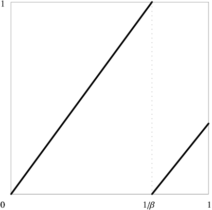
Figure 1. The $\beta$-shift

This map is very important in ergodic theory and as well as number theory, and the main tool for its study is its symbolic encoding which we are going to describe below. Note that if $\beta=d$ is an integer, then $\tau_{\beta}$ is isomorphic to the full shift on $d$ symbols. The idea suggested in [60] was to generalize this construction to the non-integer $\beta$’s.

As is well known, to “encode” it, one needs to apply the greedy algorithm in order to obtain the digits in (2.1), namely, $\varepsilon_{n}=[\beta\tau_{\beta}^{n-1}x],\ n\geq 1$. Then the one-sided shift $\sigma_{\beta}$ in the space $X_{\beta}$ of all possible sequences $\varepsilon$ that can be obtained this way, is clearly isomorphic to $\tau_{\beta}$, with the conjugating map given by (2.1). We will call $\sigma_{\beta}$ the $\beta$-shift. It is obviously a proper subshift of the full shift on $\prod_{1}^{\infty}\{0,1,\dots,[\beta]\}$. The question is, what kind of subshift is this – or equivalently – what is actually $X_{\beta}$?

This question was answered by B. Parry in the seminal paper [56]. The theorem he proved is the following. Let the sequence $(a_{n})_{1}^{\infty}$ be defined as follows: let $1=\sum_{1}^{\infty}a_{k}^{\prime}\beta^{-k}$ be the greedy expansion of 1, i.e, $a_{n}^{\prime}=[\beta\tau_{\beta}^{n-1}1],\ n\geq 1$; if the tail of the sequence $(a_{n}^{\prime})$ differs from $0^{\infty}$, then we put $a_{n}\equiv a_{n}^{\prime}$. Otherwise let $k=\max\,\{j:a_{j}^{\prime}>0\}$, and $(a_{1},a_{2},\dots):=(a_{1}^{\prime},\dots,a_{k-1}^{\prime},a_{k}^{\prime}-1)^{\infty}$.

Theorem 2.1.

[56]

1. For any sequence $(a_{n})_{1}^{\infty}$ described above, each power of its shift is lexicographically less than or equal to the sequence itself, and the equality occurs if and only if it is purely periodic. Conversely, each sequence having this property is $(a_{n}(\beta))_{1}^{\infty}$ for some $\beta>1$.

2. For each greedy expansion $(\varepsilon_{n})_{1}^{\infty}$ in base $\beta,\ (\varepsilon_{n},\varepsilon_{n+1},\dots)$ is lexicographically less (notation: $\prec$) than $(a_{1},a_{2},\dots)$ for every $n\geq 1$. Conversely, every sequence with this property is actually the greedy expansion in base $\beta$ for some $x\in[0,1)$.

Let $\mathbf{a}=(a_{n})_{1}^{\infty}$ and $\sigma$ stands for the general one-sided shift on sequences. Thus, we have

(2.2) $$X_{\beta}=\left\{\varepsilon\in\prod_{1}^{\infty}\{0,1,\dots,[\beta]\}\mid\sigma^{n}\varepsilon\prec\mathbf{a},\ n\geq 0\right\}$$

and the following diagram commutes:

$$\begin{CD}X_{\beta}@>{\sigma_{\beta}}>{}>X_{\beta}\\ @V{\pi_{\beta}}V{}V@V{}V{\pi_{\beta}}V\\ [0,1)@>{\tau_{\beta}}>{}>[0,1)\end{CD}$$

Note that usually $X_{\beta}$ is called the (one-sided) $\beta$-compactum.

Types of subshifts people know well how to deal with are mostly SFT (subshifts of finite type) and their factors, called sofic subshifts – see, e.g., [51]. It is thus natural to ask whether $X_{\beta}$ is such and if so, for which $\beta$? The following theorem gives a rather disappointing answer to this question. Roughly speaking, only certain algebraic $\beta$ yield sofic beta-compacta. Recall that an algebraic integer is called a Pisot number if it is a real number greater than 1 and all its conjugates are less than 1 in modulus. A Perron number is an algebraic integer $\beta$ greater than 1 whose conjugates are less than $\beta$ in modulus.

Theorem 2.2.

[56, 6, 50] (see also the survey [8])

1. The $\beta$-compactum $X_{\beta}$ is an SFT if and only if the sequence $a^{\prime}_{n}$ (see above) is finite (i.e., its tail is $0^{\infty}$).

2. $X_{\beta}$ is sofic if and only if $(a_{n})$ is ultimately periodic.

3. If $\beta$ is a Pisot number, then $X_{\beta}$ is sofic.

4. If $X_{\beta}$ is sofic, then $\beta$ is a Perron number.

It has to be said that a more or less explicit description of $X_{\beta}$ in case of transcendental $\beta$ (as well as for $\beta=3/2$, say) seems to be hopeless – see [8]. However, the ergodic-theoretic properties of the beta-shift are well studied and clearly understood by now for all $\beta>1$. The following statement summarizes them.

Theorem 2.3.

[60, 56, 71, 39]

1. The $\beta$-transformation is topologically mixing, and its topological entropy is equal to $\log\beta$.

2. The $\beta$-shift is intrinsically ergodic for any $\beta>1$.

3. The unique measure of maximal entropy for $\tau_{\beta}$ is equivalent to the Lebesgue measure on $[0,1]$ and the corresponding density is bounded from both sides.

4. The natural extension of $\tau_{\beta}$ is Bernoulli. Moreover, the $\beta$-shift $\sigma_{\beta}$ is weakly Bernoulli with respect to the natural (coordinate-wise) partition.

Remark 2.4.

The proof of item (2) given in [39] is rather complicated. In fact, I do not really understand why the proof of the intrinsic ergodicity of the transitive subshifts of finite type given by B. Parry (see, e.g., [79, pp. 194–196]) cannot be applied to the $\beta$-shifts as well. The only property one needs apart from ergodicity, is the fact that the measure of any cylinder of length $n$ divided by $\beta^{n}$ is uniformly bounded. This is well known since [60].

Remark 2.5.

In [7] a simplified proof of the above theorem was given. It is based on some auxiliary results on coded systems (which the $\beta$-shift is – see, e.g., [8]). Unfortunately, this manuscript, rather helpful from the methodological point of view, is unpublished and not very easy to get hold of.

The greedy expansion can be alternatively characterized as follows: assume that $n\geq 2$ and that the first $n-1$ digits of the expansion (2.1) are already chosen. Then if there is a choice for $\varepsilon_{n}$, we choose the largest possible number between 0 and $[\beta]$. Similarly, if we choose the smallest possible $\varepsilon_{n}$ every time when we have a choice, this expansion is called the lazy $\beta$-expansion. Let us formally explain what we mean by the existence of a choice. Let $r_{n}(x,\beta):=x-\sum_{1}^{n-1}\varepsilon_{k}\beta^{-k}$; if $r_{n}(x,\beta)<\beta^{-n}$, then $\varepsilon_{n}$ has be to equal to 0. If, on the contrary, $r_{n}(x,\beta)\geq[\beta]\beta^{-n}$, then inevitably $\varepsilon_{n}=[\beta]$. As is easy to see, in any other case there will be a choice for $\varepsilon_{n}$.

The following assertion is straightforward:

Lemma 2.6.

For a given $x\in[0,1)$, each of its $\beta$-expansions of the form (2.1) lies between its lazy and greedy $\beta$-expansions in the sense of lexicographic ordering of sequences.

We will return to the case of “intermediate” expansions (i.e., those that lie strictly between the lazy and greedy ones) in Section 2.3.

Remark 2.7.

As we have mentioned above, it is possible to expand any positive number (not necessarily from $(0,1)$) in base $\beta$ by means of the greedy algorithm. Namely, let $\mathbf{a}$ be as above, and

(2.3) $$\widetilde{X}_{\beta}:=\left\{\varepsilon\in\prod_{-\infty}^{\infty}\{0,1,\dots,[\beta]\}\mid(\varepsilon_{n},\varepsilon_{n+1},\dots)\prec\mathbf{a},\ n\in\mathbb{Z}\right\},$$

i.e., the natural extension of the $\beta$-compactum. We will call it the two-sided $\beta$-compactum; it will be used extensively in Section 4.

Lemma 2.8.

Any $x\geq 0$ has the greedy $\beta$-expansion of the form

(2.4) $$x=\sum_{n=-\infty}^{+\infty}\varepsilon_{n}\beta^{-n},$$

where $(\varepsilon_{n})$ is a sequence from $\widetilde{X}_{\beta}$ finite to the left, i.e., $\varepsilon_{n}\equiv 0$ for $n\leq N_{0}$ for some $N_{0}\in\mathbb{Z}$.

The proof of this claim is similar to the one on the $p$-adic representations of positive reals, and we omit it (see also Section 4).

2.2. Unique expansions and maps with gaps

This subsection is aimed to describe a branch of a relatively new direction in the theory of arithmetic expansions, which deals with lifting all restrictions on “digits” leaving only the “Cartesian hull” (see Introduction).

2.2.1. $1<\beta<2$

Assume first that $\beta\in(1,2)$ and let $\Sigma=\prod_{1}^{\infty}\{0,1\}$. In the previous subsection we have described the specific (greedy) algorithm for choosing “digits” $\varepsilon_{n}$. As we have seen, the cost for this (very natural) approach is that the set of digits is quite complicated and unless $\beta$ is an algebraic number, there is hardly any hope to describe it more or less explicitly (see Theorem 2.2).

In the 1990’s a group of Hungarian mathematicians led by Paul Erdös began to investigate 0-1 sequences that provide unique representations of reals [24, 25, 26]. More precisely, let

$$\mathcal{A}^{\prime}_{\beta}=\left\{x\in\left(0,\frac{1}{\beta-1}\right)\mid\exists!\ (\varepsilon_{n})_{1}^{\infty}\in\Sigma:x=\sum_{n=1}^{\infty}\varepsilon_{n}\beta^{-n}\right\}$$

(it is obvious that the only representation for $x=0$ is $0^{\infty}$ and the only representation for $x=1/(\beta-1)$ is $1^{\infty}$, so we will exclude both ends of the interval).

The first result about this set is given in [24]:

Proposition 2.9.

The set $\mathcal{A}^{\prime}_{\beta}$ has Lebesgue measure zero for any $\beta\in(1,2)$. Moreover, if $\beta<G$, where $G=\frac{1+\sqrt{5}}{2}$, then in fact every $x$ has $2^{\aleph_{0}}$ representations in the form (2.1).

The question is, what can one say about the cardinality and – in case it is the continuum – about the Hausdorff dimension of this set. The answer to this question is given by P. Glendinning and the author in [32].

To present this result, we need some preliminaries. Let $\beta_{*}$ denote the Komornik-Loreti constant introduced by V. Komornik and P. Loreti in [44], which is defined as the unique solution of the equation

$$\sum_{1}^{\infty}\mathfrak{m}_{n}x^{-n+1}=1,$$

where $\mathfrak{m}=(\mathfrak{m}_{n})_{1}^{\infty}$ is the Thue-Morse sequence

$$\mathfrak{m}=0110\,\,1001\,\,1001\,\,0110\,\,1001\,\,0110\dots,$$

i.e., the fixed point of the substitution $0\to 01,\ 1\to 10$. The Komornik-Loreti constant is known to be transcendental [4], and its numerical value is approximately as follows:

$$\beta_{*}=1.787231650\dots$$

The reason why this constant was introduced in [44] is that it proves to be the smallest number $\beta$ such that $x=1$ has a unique representation in the form (2.1). Now we are ready to formulate the result we mentioned above.

Theorem 2.10.

[32] The set $\mathcal{A}^{\prime}_{\beta}$ is:

• empty if $\beta\in(1,G]$;

• countable for $\beta\in(G,\beta_{*})$;

• an uncountable Cantor set of zero Hausdorff dimension if $\beta=\beta_{*}$; and

• a Cantor set of positive Hausdorff dimension for $\beta\in(\beta_{*},2)$.

The proof of this result given in [32] is based on the observation that for $\varepsilon$ to be a unique expansion for some $x\in\left(\frac{2-\beta}{\beta-1},1\right)$, it has to be its both greedy and lazy expansion – this is a direct consequence of Lemma 2.6. Let $\mathcal{A}_{\beta}=\mathcal{A}^{\prime}_{\beta}\cap\left(\frac{2-\beta}{\beta-1},1\right)$ and $\mathcal{U}_{\beta}=\pi_{\beta}^{-1}(\mathcal{A}_{\beta})$, where $\pi_{\beta}$ is given by (2.1). It suffices to use (2.2) and a similar condition for the lazy expansion, which leads to the following lemma on the structure of the set $\mathcal{U}_{\beta}$:

Lemma 2.11.

[32] The set $\mathcal{U}_{\beta}$ can be described as follows:

(2.5) $$\mathcal{U}_{\beta}=\{\varepsilon\in\Sigma:\overline{\mathbf{a}}\prec\sigma^{n}\varepsilon\prec\mathbf{a},\ n\geq 0\}.$$

Remark 2.12.

It is worth noting that although (2.2) looks similar to (2.5), the compacta $X_{\beta}$ and $\mathcal{U}_{\beta}$ are completely different. In particular, the entropy of the $\beta$-shift is $\log\beta$ and in the case of the shift on $\mathcal{U}_{\beta}$ it is constant a.e. – see Theorem 2.14 below. Note also that restrictions like (2.5) are quite common in one-dimensional dynamics, and this is not a coincidence – see [33].

From Lemma 2.11 one can obtain the result on the cardinality of $\mathcal{U}_{\beta}$ and therefore of $\mathcal{A}_{\beta}^{\prime}$ as well – see [32].

The problem with this proof is that it may be characterized as “a rabbit out of a hat” type of proof. Indeed, it does not say anything about the origin of the Komornik-Loreti constant as the main threshold between countable and uncountable set of uniquely representable points. This collision was overcome in the subsequent papers by the same authors [33, 34].

The key paper [33] is devoted to a “dynamical” version of the proof which will also involve various ergodic-theoretic and geometric applications for the shift on the space $\mathcal{U}_{\beta}$. Let us explain, where dynamics enters the game.

In a number of recent works maps with gaps or a maps with holes have been considered – see, e.g., [12] and references therein. The model in question is as follows: let $X\subset\mathbb{R}^{d}$ and $f:X\to X$ be a map (invertible or not) with positive topological entropy. Let $D$ be an open subset of $X$. The idea is to study the “dynamics of $f$ on $X\setminus D$”. More precisely, let

$$U=X\setminus\bigcup_{n\in\mathbb{Z}}f^{n}(D)\quad\textrm{if $f$ is invertible}$$

or

$$U=X\setminus\bigcup_{n\leq 0}f^{n}(D)\quad\textrm{if $f$ is non-invertible}.$$

One may ask two questions about this model.

Question 1. Is $U$ empty? countable? uncountable? a Cantor set of positive Hausdorff dimension?

Question 2. If $U$ has positive Hausdorff dimension, describe the dynamics of $f_{U}=f|_{U}$ (sometimes called the exclusion map). For instance, is $f_{U}$ transitive? topologically mixing? intrinsically ergodic? etc.

Some (mostly, “generic” results) in this direction for Axiom A maps $f$ on smooth manifolds can be found in [14, 15, 16, 12]. In particular, in [12] it is shown that if $f$ is a hyperbolic algebraic automorphism of the torus $\mathbb{T}^{m}$ (see Section 4 for the relevant definitions) and $D=D(a_{1},\dots,a_{m})$ is the parallelepiped built along the leaves of the stable and unstable foliation of $f$ passing through $\mathbf{0}$ with the sides of length $a_{1},\dots,a_{m}$, then for a Lebesgue-generic $m$-tuple $(a_{1},\dots,a_{m})$ the exclusion map $f|_{U}$ is a subshift of finite type.

Return to our situation. Let $T_{\beta}$ be the following “map with a gap” acting from $[0,1/(\beta-1)]$ onto itself:

(2.6) $$T_{\beta}(x)=\begin{cases}\beta x,&x\in\bigl{[}0,\frac{1}{\beta}\bigr{]}\\ \textrm{not defined},&x\in\bigl{(}\frac{1}{\beta},\frac{1}{\beta(\beta-1)}\bigr{)}\\ \beta x-1,&x\in\bigl{[}\frac{1}{\beta(\beta-1)},\frac{1}{\beta-1}\bigr{]}\end{cases}$$

(see Figure 2).

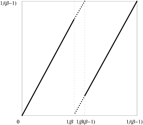
Figure 2. The map with a gap $T_{\beta}$

The following simple lemma relates the dynamics of $T_{\beta}$ to the original problem. Let

$$\Delta_{\beta}=[1/\beta,1/\beta(\beta-1)].$$

Lemma 2.13.

[33]

$$\mathcal{A}^{\prime}_{\beta}=\left\{x\in\left(0,\frac{1}{\beta-1}\right):T_{\beta}^{n}(x)\notin\Delta_{\beta}\,\textrm{for all}\,\,n\geq 0\right\}.$$

Proof.

Note first that if $x\in[0,1/\beta)$, then necessarily $\varepsilon_{1}$ in (2.1) is 0 and if $x\in(1/\beta(\beta-1),1/(\beta-1))$, then it is necessarily 1. If it belongs to $\Delta_{\beta}$, then there is always at least two different representations.

Let $S_{\beta}$ denote the shift on $\mathcal{U}_{\beta}$ and $R_{\beta}=T_{\beta}|_{\mathcal{A}_{\beta}}$. Then the following commutative diagram takes place:

$$\begin{CD}\mathcal{U}_{\beta}@>{S_{\beta}}>{}>\mathcal{U}_{\beta}\\ @V{\pi_{\beta}}V{}V@V{}V{\pi_{\beta}}V\\ \mathcal{A}_{\beta}@>{R_{\beta}}>{}>\mathcal{A}_{\beta}\end{CD}$$

Thus, $T_{\beta}$ acts as a shift on sequences providing unique representations. Indeed, it is either $x\mapsto\beta x$ or $\beta x-1$ depending on whether we have $\varepsilon_{1}=0$ or 1, which is precisely the shift in (2.1). Hence for a $T_{\beta}$-orbit to stay out of $\Delta_{\beta}$ at any iteration is the same as keeping the representation (2.1) unique. ∎

The important problem now is to describe the topological and ergodic properties of the shift $S_{\beta}$. The following theorem summarizes all we know at present about them.

Theorem 2.14.

[33]

1. For every $\beta\in(\beta_{*},2)$ the subshift $S_{\beta}$ is essentially transitive, i.e., has a unique transitive component of maximal entropy.

2. The shift $S_{\beta}$ is a subshift of finite type for a.e. $\beta$.

3. For a.e $\beta\in(\beta_{*},2)$ the subshift $S_{\beta}$ is intrinsically ergodic and metrically isomorphic to a transitive SFT.

4. The function $\beta\mapsto h_{top}(\sigma_{\beta})$ is continuous (but not Hölder continuous) and constant a.e. Every interval of constancy is naturally parameterized by an algebraic integer of a certain class.

The open question is whether the shift $S_{\beta}$ is “as good as” the beta-shift $\sigma_{\beta}$ (see above). Namely, we conjecture that for any $\beta\in(\beta_{*},2)$ it is intrinsically ergodic and its natural extension is Bernoulli.

Remark 2.15.

The above family of maps with gaps as a dynamical object might look artificial: we change not only the slope but the gap as well. However, if one alters the size of gap only (which is more conventional), then the result on the symbolic level will be essentially the same. For example, let $Tx=2x\bmod 1$ and $D_{\delta}=[\delta,1-\delta]$ for $\delta\in(0,1/2)$. Let now

$$\mathcal{K}_{\delta}=\{x\in(0,1):T^{n}(x)\notin D_{\delta},\ n\geq 0\}.$$

It is known from the physical literature that $\dim_{H}(\mathcal{K}_{\delta})>0$ if and only if $\delta>\sum_{1}^{\infty}\mathfrak{m}_{n}2^{-n}=0.412\dots$ (this has been apparently shown independently in [9, 81]). From the above results this claim follows almost immediately. Sketch of the proof of this fact is as follows: let $\mathbf{a}$ denote the binary expansion of $2\delta$; then in terms of the full 2-shift the set $\mathcal{K}_{\delta}$ is defined by (2.5); the only difference with $\mathcal{U}_{\beta}$ is that the sequence $\mathbf{a}$ does not necessarily satisfy the condition from Theorem 2.1 (1), but this is easy to deal with. So, the shifted Thue-Morse sequence is critical as well, which leads to the result in question. For a more general case see [33].

2.2.2. $\beta>2$

Assume now that $\beta\in(N,N+1)$ for some $N\geq 2$; we have similar results with some natural analog of the Thue-Morse sequence. Namely, let $\rho$ denote the following substitution (morphism):

$$a\to ac,\,\ b\to ad,\,\,c\to da,\,\,d\to db.$$

Then

$$\rho^{\infty}(d)=:(\mathfrak{w}_{n})_{1}^{\infty}=dbabacdb\dots$$

The sequence $(\mathfrak{w}_{n})_{1}^{\infty}$ is related to the Thue-Morse sequence in the following way:

$$\sigma(\mathfrak{m})=\underbrace{1101}_{d}\,\,\underbrace{0011}_{b}\,\,\underbrace{0010}_{a}\,\,\underbrace{1101}_{d}\,\,\underbrace{0010}_{a}\,\,\underbrace{1100}_{c}\,\,\underbrace{1101}_{d}\,\,\underbrace{0011}_{b}\dots$$

Let $P_{n}:\{0,1\}\to\{n-1,n\}$ be defined by

$$P_{n}(0)=n-1,\ P_{n}(1)=n$$

and $Q_{n}:\{a,b,c,d\}\to\{n-1,n,n+1\}$:

$$Q_{n}(a)=n-1,\ Q_{n}(b)=Q_{n}(c)=n,\ Q_{n}(d)=n+1.$$

Then the critical value $x=\beta_{*}^{(N)}$ analogous to $\beta_{*}$ is given by the equations

$$1=\sum_{k=1}^{\infty}P_{n}(\mathfrak{m}_{k+1})x^{-k},\quad N=2n,\ n\geq 1$$

or

$$1=\sum_{k=1}^{\infty}Q_{n}(\mathfrak{w}_{k})x^{-k},\quad N=2n+1,\ n\geq 1.$$

More precisely, let $\mathcal{A}_{\beta}^{(N)}$ denote the set of $x$ which have a unique $\beta$-expansion with the digits $0,1,\dots,N-1$.

Theorem 2.16.

[34]

1. The number $\beta_{*}^{(N)}$ is the smallest $\beta$ for which $x=1$ has a unique $\beta$-expansion with the digits $0,1,\dots,N-1$.

2. The set $\mathcal{A}_{\beta}^{(N)}$ has positive Hausdorff dimension if and only if $\beta>\beta_{*}^{(N)}$. If $\beta<\beta_{*}^{(N)}$, then it is at most countable.

Remark 2.17.

The method of proving this type of theorems comes from low-dimensional dynamics: it is called renormalization. For more detailed results in this direction and discussion see [33, 34].

2.3. Intermediate beta-expansions

Assume for simplicity that $\beta<2$ and have another look at the map with a gap $T_{\beta}$ defined above. More precisely, let

(2.7) $$T^{\prime}_{\beta}(x)=\begin{cases}\beta x,&x\in\bigl{[}0,\frac{1}{\beta(\beta-1)}\bigr{]}\\ \beta x-1,&x\in\bigl{[}\frac{1}{\beta},\frac{1}{\beta-1}\bigr{]}.\end{cases}$$

Thus, we have a multivalued map on the middle interval $\Delta_{\beta}$, and in order to get a “normal” (single-valued) map, one needs to make a choice for every $x\in\Delta_{\beta}$. From this point of view the $\beta$-shift corresponds to the choice of the lower branch and the “lazy” $\beta$-shift – the higher one for every $x$. On the other hand, as we have seen, if one removes the middle interval completely, then this corresponds to the unique expansions and eventually to the map that acts on at most a Cantor set, namely, $T_{\beta}|_{\mathcal{A}_{\beta}}$.

In [17] K. Dajani and C. Kraaikamp suggested the idea of considering “intermediate” beta-expansions, or how they called them, $(\beta,\alpha)$-expansions. More precisely, let $\alpha$ be our parameter, $\alpha\in[0,(2-\beta)/(\beta-1)]$. We choose the upper branch if the ordinate is less than $1+\alpha$ and the lower branch otherwise, then restrict the resulting map to the interval $[\alpha,1+\alpha]$. Thus, we get

$$T_{\beta,\alpha}(x)=\begin{cases}\beta x,&x\in\bigl{[}\alpha,\frac{1+\alpha}{\beta}\bigr{)}\\ \beta x-1,&x\in\bigl{[}\frac{1+\alpha}{\beta},1+\alpha\bigr{]}.\end{cases}$$

(see Figure 3).

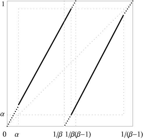
Figure 3. The pattern for the $(\beta,\alpha)$-expansion

As is easy to see, $T_{\beta,\alpha}$ is isomorphic to the map $S_{\beta,\gamma}:[0,1)\to[0,1)$ acting by the formula

$$S_{\beta,\gamma}(x)=\beta x+\gamma\bmod 1,\quad\gamma=(\beta-1)\alpha\in[0,2-\beta].$$

The ergodic properties of the family $S_{\beta,\gamma}$ are well studied, see, e.g., [57, 40, 27]. In particular, $S_{\beta,\gamma}$ is ergodic with respect to the Lebesgue measure, which is equivalent to the measure of maximal entropy.

2.4. The realm of beta-expansions

In the previous subsections we have studied the beta-expansions from the viewpoint of choosing a specific representation for a given $x$ in (2.1) (and for $x\in\mathcal{A}^{\prime}_{\beta}$ this choice was unique). We believe it is interesting to study the space of all possible representations of a given $x$, which this subsection will be devoted to.

So, let $\beta>1$ be fixed, and $\Sigma_{q}=\prod_{1}^{\infty}\{0,1,\dots,q-1\}$ for some fixed $q\geq 2$. We define for any $x\geq 0$,

$$\mathfrak{R}_{\beta,q}(x):=\left\{\varepsilon\in\Sigma_{q}:x=\sum_{n=1}^{\infty}\varepsilon_{n}\beta^{-n}\right\}.$$

In the case when $\beta$ is non-integer, and $q=[\beta]+1$, we will simply write $\mathfrak{R}_{\beta}(x)$.

Not much is known about the general case yet. The following result was obtained by the author [67] by elementary means. In this paper we would like to present an ergodic-theoretic proof that may possibly start the whole new line of research in this area (see Remark 2.20 below). The author is grateful to V. Komornik for his help with the history of the issue.

Theorem 2.18.

For any $\beta\in(1,2)$ the cardinality of $\mathfrak{R}_{\beta}(x)$ is the continuum for a.e. $x\in(0,1/(\beta-1))$.

Proof.

Recall that if $\beta<G$, then every point $x$ is known to have $2^{\aleph_{0}}$ $\beta$-expansions [25, Theorem 3]. So, let $\beta\geq G$.

By the above, it suffices to show that

(2.8) $$\textrm{card}\,\left(\bigcup_{n=1}^{\infty}(T_{\beta}^{\prime})^{n}(x)\right)=2^{\aleph_{0}}$$

for a.e. $x\in(0,1/(\beta-1))$ (where $T_{\beta}^{\prime}$ is the multivalued map given by (2.7)). Let

$$T_{0}(x)=\begin{cases}\beta x,&x\in\bigl{[}0,\frac{1}{\beta(\beta-1)}\bigr{)}\\ \beta x-1,&x\in\bigl{[}\frac{1}{\beta(\beta-1)},\frac{1}{\beta-1}\bigr{)}\end{cases}$$

and

$$T_{1}(x)=\begin{cases}\beta x,&x\in\bigl{[}0,\frac{1}{\beta}\bigr{)}\\ \beta x-1,&x\in\bigl{[}\frac{1}{\beta},\frac{1}{\beta-1}\bigr{)}\end{cases}$$

(we omit the index $\beta$ to simplify our notation). Then $T_{\beta}^{\prime}x=T_{0}x\cup T_{1}x$ for any $x\in\Delta_{\beta}$, whence any point $y$ of the union in (2.8) is of the form

(2.9) $$x_{n}=T_{0}^{k_{n}}T_{1}^{k_{n-1}}\dots T_{1}^{k_{2}}T_{0}^{k_{1}}(x),$$

where $k_{j}\geq 0,1\leq j\leq n$. We are going to show that for a Lebesgue-generic $x$ and every $x_{n}$ of the form (2.9) there exists $k_{n+1}\in\mathbb{N}$ such that $T_{\beta}^{k_{n+1}}(x_{n})\in\Delta_{\beta}$ (where $T_{\beta}$ is given by (2.6)), i.e., the branching for the multivalued map $T_{\beta}^{\prime}$ has the form of the binary tree for a.e. $x$.

Fix the vector $(k_{1},\dots,k_{n})\in\mathbb{Z}_{+}^{n}$ and let within this proof

$$T:=T_{0}^{k_{n}}T_{1}^{k_{n-1}}\dots T_{1}^{k_{2}}T_{0}^{k_{1}}.$$

Following the canonical proof of the corollary to the Poincaré Recurrence Theorem (saying that a generic point returns to a given set of positive measure infinitely many times), we will show that for a.e. $x$ there exists $m\in\mathbb{N}$ such that $T^{m}(x)\in\Delta_{\beta}$. This will prove the claim of our Theorem: let $E(k_{1},\dots,k_{n})$ denote the generic set in question; then

$$E:=\bigcap_{\begin{subarray}{c}n\geq 1\\ (k_{1},\dots,k_{n})\in\mathbb{Z}_{+}^{n}\end{subarray}}E(k_{1},\dots,k_{n})$$

will be a sought set of full measure.

So, it suffices to show that

$$\mathcal{L}\left(\bigcup_{j=1}^{\infty}T^{-j}\Delta_{\beta}\right)=1$$

(where $\mathcal{L}$ is the normalized Lebesgue measure on $[0,1/(\beta-1)]$). But since $T_{0}$ and $T_{1}$ are both extensions of $T_{\beta}$, we have $T^{-1}A\supset T_{\beta}^{-p}A$ for every measurable $A$ with $p=k_{1}+\dots+k_{n}$. It is thus left to show that

(2.10) $$\mathcal{L}\left(\bigcup_{j=1}^{\infty}T_{\beta}^{-pj}\Delta_{\beta}\right)=1$$

for every $p\geq 1$. Let

$$\widetilde{T}_{\beta}(x)=\begin{cases}\beta x,&x\in\bigl{[}0,\frac{1}{\beta}\bigr{]}\\ 1,&x\in\bigl{(}\frac{1}{\beta},\frac{1}{\beta(\beta-1)}\bigr{)}\\ \beta x-1,&x\in\bigl{[}\frac{1}{\beta(\beta-1)},\frac{1}{\beta-1}\bigr{]}.\end{cases}$$

Thus, $\widetilde{T}_{\beta}$ is a “real map”; however, it is obvious that preimage-wise the maps $T_{\beta}$ and $\widetilde{T}_{\beta}$ are the same. Moreover, the normalized Lebesgue measure on $[0,1/(\beta-1)]$ is quasi-invariant under $\widetilde{T}_{\beta}$; similarly to [60] and [57], one can easily show that there exists a unique $\widetilde{T}_{\beta}$-invariant measure $\mathcal{L}_{\beta}$ which is equivalent to the Lebesgue measure. Thus, the measure $\mathcal{L}_{\beta}$ is $(\widetilde{T}_{\beta})^{p}$-invariant as well, which by the Poincaré Recurrence Theorem implies (2.10), and we are done. ∎

Remark 2.19.

It is easy to generalize this theorem to the case of an arbitrary non-integer $\beta>1$ and arbitrary $q>[\beta]$. We leave the details for the reader as a simple exercise (note: it is sufficient to consider the case $q=[\beta]+1$).

Remark 2.20.

The branching for $T_{\beta}^{\prime}$ described in the proof of the theorem, may be apparently studied in a more quantitative way. In particular, we conjecture that not only the cardinality of $\mathfrak{R}_{\beta}(x)$ is the continuum for a generic $x$ but its Hausdorff dimension in the space $\Sigma$ (provided with the natural ($=$ binary) metric) is positive. This might be possibly shown by studying the average return times to the set $\Delta_{\beta}$ for the multivalued map $T_{\beta}^{\prime}$ and will be considered elsewhere.

Example 2.21.

Let $\beta=G$; it is shown in [68, Appendix A] that $\mathfrak{R}_{G}(x)$ is always a continuum unless $x=nG\bmod 1$ for some $n\in\mathbb{Z}$. For example, $\mathfrak{R}_{G}(1/2)=\prod_{1}^{\infty}\{011,100\}$, whence it is indeed a continuum, and its Hausdorff dimension equals $\frac{1}{3}$.

An important special case is when $\beta$ is a Pisot number (see Section 2.1 for definition). Then one may study the combinatorics of the infinite space by means of the combinatorics of its finite approximations. More precisely, let us call two sequences $\varepsilon$ and $\varepsilon^{\prime}$ from $\Sigma_{q}$ equivalent if $\sum_{1}^{\infty}\varepsilon_{k}\beta^{-k}=\sum_{1}^{\infty}\varepsilon^{\prime}_{k}\beta^{-k}$. There are a number of results about counting the cardinality of equivalence classes; most of them deal with random matrix products [46, 45, 55]. In particular, it is shown in [45] that for a generic 0-1 sequence $(x_{n})_{1}^{\infty}$ the cardinality of the equivalence class of $(x_{1}\dots x_{n})$ grows with $n$ exponentially with an exponent greater than 1. The value of this exponent is given by the upper Lyapunov exponent of the random matrix product in question.

One special case is however worth mentioning on its own. Let $\beta=G$ (the golden ratio) and $q=2$. We call a finite 0-1 word a block if it begins with 1 and ends by an even number of 0’s. As is easy to show by induction, every block has the following form:

$$B=1(01)^{a_{1}}(00)^{a_{2}}\dots(00)^{a_{r}}\quad\mathrm{or}\quad B=1(00)^{a_{1}}(01)^{a_{2}}\dots(00)^{a_{r}}.$$

Hence each block $B$ is parameterized in a unique way by the natural numbers $a_{1},\dots,a_{r}$. We will write $B=B(a_{1},\dots,a_{r})$. Let $\mathfrak{c}(w)$ denote the cardinality of the set of all 0-1 words equivalent to $w$.

In 1998 the author together with A. Vershik proved the following

Theorem 2.22.

[68]

1. Let $w=B_{1}\dots B_{k}$, where $B_{j}$ is a block for all $j$. Then the space of all 0-1 words equivalent to $w$ splits into the Cartesian product of the equivalence classes for $B_{j}$ for $j=1$ to $k$, and therefore, the function $\mathfrak{c}$ is blockwise multiplicative:

   $$\mathfrak{c}(B_{1}\dots B_{k})=\mathfrak{c}(B_{1})\dots\mathfrak{c}(B_{k}).$$

2. The cardinality of a block is given by the formula

   $$\mathfrak{c}(B)=p_{r}+q_{r},$$

   where $\frac{p_{r}}{q_{r}}=[a_{1},\dots,a_{r}]$ is the continued fraction.

The proof given in [68] is based on an induction argument; however, now it is clear that there exists a more direct and elegant way of proving this result. Let $X=X_{G}$ which in this case is the Markov compactum of all 0-1 sequences without two consecutive 1’s and let $g:\prod_{1}^{\infty}\{a,b,c\}\to X$ act by the following rule:

$$g(a)=00,\ g(b)=010,\ g(c)=10$$

and then by concatenation.

Lemma 2.23.

The map $g$ is a bijection.

Proof.

It is a straightforward check that $g^{-1}$ is well defined: any sequence from $X$ can be split in a unique way into the concatenation of the blocks $00,010$ and $10$. ∎

Let $w$ be a finite word in $X$ and $g^{-1}w=j_{1}\dots j_{m}$. In [55] it was shown that

$$\mathfrak{c}(w)=\begin{pmatrix}1&0\end{pmatrix}P_{j_{1}}P_{j_{2}}\dots P_{j_{m}}\begin{pmatrix}1\\ 0\end{pmatrix},$$

where

$$P_{a}=\begin{pmatrix}1&1\\ 0&1\end{pmatrix},\quad P_{b}=\frac{1}{2}\begin{pmatrix}1&1\\ 1&1\end{pmatrix},\quad P_{c}=\begin{pmatrix}1&0\\ 1&1\end{pmatrix}.$$

This immediately yields both parts of Theorem 2.22, in view of the well-known relation between the matrix products of $P_{a}$ and $P_{c}$ and the finite continued fractions. The details are left to the reader.

The main consequence of Theorem 2.22 is the existence of the map called the goldenshift which acts on sequences from $X$ starting with 1 as the shift by the length of the first block. This goldenshift is well defined a.e. and has a number of important properties that reveal a lot of information about the Bernoulli convolution parameterized by the golden ratio. For details see [68, §§2, 3].

Remark 2.24.

In [68, Appendix A] A. Vershik and the author completely described all the possible patterns for $\mathfrak{R}_{G}(x)$ if $x\in(0,1)$. Loosely speaking, these possibilities are as follows: either $\mathfrak{R}_{G}(x)$ is a Cartesian product (this is Lebesgue-generic – see also Example 2.21) or $\mathfrak{R}_{G}(x)=\mathcal{X}_{\alpha}^{\prime}$ for a certain $\alpha=\alpha(x)$, where $\mathcal{X}_{\alpha}^{\prime}$ is the “rotational” Markov compactum described in the next section. For more general Pisot numbers the analog of this theorem seems to be a delicate and interesting problem.

Remark 2.25.

The combinatorics of the “integral” case $\beta\in\mathbb{N}$ is studied in detail by J.-M. Dumont, A. Thomas and the author in [19, §6]. In that case the cardinality function can be represented in terms of random matrix products as well. Specifically, if $\beta=2$ and $q=3$, then these matrices are precisely $P_{a}$ and $P_{c}$.

Remark 2.26.

There exists a class of singular measures (Bernoulli convolutions) that are based on the combinatorics we have just described. For more details see, e.g., [3, 68] for the case of $\beta=G$ and [23, 31, 46, 45, 55] for more general cases of Pisot numbers (see also the survey article [58] for a general overview).

3. Rotational expansions

In this section we are going to describe the model appeared first in [73] as an application of the general theorem by A. Vershik on adic realization – see Theorem 4.34 in Appendix, and in a more arithmetic form – in the joint paper [77] by A. Vershik and the author. Also, we will present another model which deals with more conventional base for arithmetic expansions.

3.1. General constructions

3.1.1. First model

The problem we are going to consider in this section, is arithmetic codings of an irrational rotation of the circle $\mathbb{R}/\mathbb{Z}$ which we will identify with the interval $[0,1)$. Let $\alpha\in(0,1/2)\setminus\mathbb{Q}$ be the angle of rotation (if it is greater than $1/2$, simply take $1-\alpha$), and let $\mathcal{R}_{\alpha}(x)=x+\alpha\bmod 1$. Let the regular continued fraction expansion of $\alpha$ be

$$\alpha=\cfrac{1}{a_{1}+\cfrac{1}{a_{2}+\cfrac{1}{a_{3}+\dots}}}$$

and $(p_{n}/q_{n})_{1}^{\infty}$ be the sequence of convergents with $p_{1}=0,p_{1}=1,q_{1}=1,q_{2}=a_{1}$ and $p_{n+1}=a_{n}p_{n}+p_{n-1},q_{n+1}=a_{n}q_{n}+q_{n-1}$. Since $\alpha<1/2$, we have $a_{1}\geq 2$. Put $r_{1}=a_{1},r_{n}=a_{n}+1,n\geq 2$ and,

$$M^{(n)}=M^{(n)}(\alpha):=\begin{pmatrix}1&\dots&1&1\\ 1&\dots&1&0\\ \vdots&\vdots&\vdots&\vdots\\ 1&\dots&1&0\end{pmatrix},$$

where the number of rows in $M^{(n)}$ is $r_{n}$, and the number of columns is $r_{n+1}$. Let $D_{n}=\{0,1,\dots,r_{n}-1\}$ be endowed with the natural ordering, i.e., $0\prec 1\prec\cdots\prec r_{n}-1$. Let now $\mathcal{X}_{\alpha}$ denote the Markov compactum determined by the sequence of matrices $(M^{(n)}(\alpha))_{1}^{\infty}$ and $\mathcal{T}_{\alpha}$ denote the adic transformation on $\mathcal{X}_{\alpha}$ with respect to the natural ordering (see Appendix for the definitions).

Note first that $\mathcal{T}_{\alpha}$ is well defined everywhere with the exception of two “maximal” sequences: $(a_{1}-1,0,a_{3},0,a_{5},\dots)$ and $(0,a_{2},0,a_{4},0,\dots)$. Thus, if we exclude the cofinite sequences (i.e., those whose tail is $(a_{n},0,a_{n+2},0,\dots)$ for some $n$), the positive part of the orbit of $\mathcal{T}_{\alpha}$ will be always well defined. To enable the whole trajectory of $\mathcal{T}_{\alpha}$ to be well defined, one has to remove the finite sequences as well.

We claim that the map $\mathcal{T}_{\alpha}$ is metrically isomorphic to $\mathcal{R}_{\alpha}$ and are going to present the conjugating map. Let $\psi_{\alpha}:\mathcal{X}_{\alpha}\to[0,1)$ be defined as

(3.11) $$\psi_{\alpha}(x_{1},x_{2},\dots):=\alpha+\sum_{n=1}^{\infty}x_{n}(-1)^{n+1}\alpha_{n},$$

where $\alpha_{n}=|q_{n}\alpha-p_{n}|=\|q_{n}\alpha\|$ (here $\|\cdot\|$ stands for the distance to the nearest integer).

Theorem 3.1.

[77]

1. The invertible dynamical system $(\mathcal{X}_{\alpha},\mathcal{T}_{\alpha})$ is uniquely ergodic. The unique invariant measure $\nu_{\alpha}$ is Markov on $\mathcal{X}_{\alpha}$.

2. $\psi_{\alpha}$ is continuous and one-to-one except the cofinite sequences.

3. The map $\psi_{\alpha}$ metrically conjugates the automorphisms $(\mathcal{X}_{\alpha},\nu_{\alpha},\mathcal{T}_{\alpha})$ and $([0,1),\mathcal{L},\mathcal{R}_{\alpha})$, where $\mathcal{L}$ stands for the Lebesgue measure on the unit interval.

Remark 3.2.

As is well known, $\alpha_{n}$ decays at a very fast rate as $n$ goes to the infinity, namely, $\alpha_{n}=O(q_{n+1}^{-1})$ (see, e.g., [43]). Thus, the $n$’th term of the sum in (3.11) is $O(q_{n}^{-1})$, i.e., decays at worst exponentially.

Remark 3.3.

Expansion (3.11) was considered for the first time by Y. Dupain and V. Sos [20]; they also proved Theorem 3.1 (2), the fact A. Vershik and the author were unaware of when writing [77]. This however hardly undermines Theorem 3.1 as it appeared in [77], because the (most important) dynamical meaning of the rotational expansion was new.

Remark 3.4.

A simple way to obtain these expansions is as follows: let $N\in\mathbb{N}$ and $(q_{n})_{1}^{\infty}$ serve as a “base” for representations in the sense of [28]. Then there is a unique representation of $N$ in the form

(3.12) $$N=1+\sum_{k}x_{k}q_{k},$$

where $(x_{1},x_{2},\dots)$ is a finite sequence in $\mathcal{X}_{\alpha}$. All one has to do to get (3.11) is to make a profinite completion of (3.12) using the fact that the sequence $(N\alpha\bmod 1)_{1}^{\infty}$ is dense in $[0,1)$ and the formula $q_{k}-p_{k}\alpha=(-1)^{k+1}\alpha_{k}$. For more details see [77, §2].

Remark 3.5.

If one removes both the finite and cofinite sequences from $\mathcal{X}_{\alpha}$ and the $\mathcal{T}_{\alpha}$-trajectory of 0 from $[0,1)$, then $\psi_{\alpha}$ becomes a homeomorphism and thus, acts as a conjugacy in the topological sense as well.

3.1.2. Second model

The price we pay for the natural ordering in the first model is that the base of the expansions is not always positive. The second model we are going to describe below, overcomes this problem but here there is the price to pay as well: the ordering is rather unusual. Apparently, it is impossible to take care of both issues simultaneously – this symbolizes the well-known fact that the convergents $(p_{n}/q_{n})<\alpha$ if $n$ is even and $>\alpha$ if $n$ is odd.

Let $\alpha\in(0,1)\setminus\mathbb{Q}$ and

$$\mathcal{M}^{(n)}=\mathcal{M}^{(n)}(\alpha):=\begin{pmatrix}1&1&\dots&1&1\\ \dots&\dots&\dots&\dots&\dots\\ 1&1&\dots&1&1\\ 1&0&\dots&0&0\\ \end{pmatrix},$$

where the size of $\mathcal{M}^{(n)}$ is $(a_{n}+1)\times(a_{n+1}+1)$. Let $\mathcal{D}_{n}=\{0,1,\dots,a_{n}\}$. We define the alternating ordering on $\mathcal{D}_{n}$ as follows: $0\prec 1\prec\cdots\prec a_{n}$ if $n$ is odd and $0\succ 1\succ\cdots\succ a_{n}$ if $n$ is even.

Let now $\mathcal{X}^{\prime}_{\alpha}$ denote the corresponding Markov compactum, $\mathcal{T}^{\prime}_{\alpha}$ – the adic transformation on it and $\psi^{\prime}_{\alpha}:\mathcal{X}^{\prime}_{\alpha}\to[0,1)$ be defined as follows:

(3.13) $$\psi^{\prime}_{\alpha}(x_{1},x_{2},\dots):=\sum_{n=1}^{\infty}x_{n}\alpha_{n},$$

where $\alpha_{n}$ are as above. We have the following analog of Theorem 3.1:

Theorem 3.6.

[77]

1. The map $\mathcal{T}^{\prime}_{\alpha}$ is well defined everywhere except the sequence $(a_{1},0,a_{3},\linebreak[1]0,\dots)$. Its inverse is not well defined only at $(0,a_{2},0,a_{4},0,\dots)$.

2. The dynamical system $(\mathcal{X}^{\prime}_{\alpha},\mathcal{T}^{\prime}_{\alpha})$ is uniquely ergodic. The unique invariant measure $\mu_{\alpha}$ is Markov on $\mathcal{X}_{\alpha}^{\prime}$.

3. $\psi^{\prime}_{\alpha}$ is continuous and one-to-one except the cofinite sequences.

4. The map $\psi^{\prime}_{\alpha}$ metrically conjugates the automorphisms $(\mathcal{X}_{\alpha}^{\prime},\mu_{\alpha},\mathcal{T}_{\alpha}^{\prime})$ and $([0,1),\mathcal{L},\mathcal{R}_{\alpha})$.

Remark 3.7.

The expansion (3.13) is a special case of the general class of Cantor-Waterman expansions [80]. More general systems of numeration are considered in [77] as well but without clear dynamical meaning.

Remark 3.8.

An analog of (3.12) for the integers is as follows:

(3.14) $$N=\sum_{n}x_{n}(-1)^{n}q_{n},$$

where $N\in\mathbb{Z}$ (not necessarily nonnegative!) and $(x_{n})$ is a finite sequence from $\mathcal{X}_{\alpha}^{\prime}$ [77]. Thus, the alternating base is not for the reals but for the integers in the second model. Comparing (3.11) with (3.13) and (3.12) with (3.14), we see that the two models are in a way dual.

3.2. Probabilistic properties of the “digits”

In this subsection we are going to mention briefly the results from [63] on Laws of Large Numbers (LLN and SLLN) and the Central Limit Theorem (CLT) for the sequences of digits for the expansions considered above. We will consider the metric space $(\mathcal{X}_{\alpha}^{\prime},\mu_{\alpha})$; the results for $(\mathcal{X}_{\alpha},\nu_{\alpha})$ are very similar, so we will omit them.

First, the initial distribution for $\mu_{\alpha}$ is as follows:

$$\mu_{\alpha}(x_{1}=i_{1})=\begin{cases}\alpha,&x_{1}<a_{1}\\ \alpha_{2},&x_{1}=a_{1},\end{cases}$$

the transition probabilities are given by

(3.15) $$\mu_{\alpha}\big{(}x_{n}=i_{n}\mid x_{n-1}=i_{n-1}\big{)}=\begin{cases}\frac{\alpha_{n}}{\alpha_{n-1}},&i_{n-1}<a_{n-1},\quad i_{n}<a_{n}\\ \frac{\alpha_{n+1}}{\alpha_{n-1}},&i_{n-1}<a_{n-1},\quad i_{n}=a_{n}\\ 1,&i_{n-1}=a_{n-1},\quad i_{n}=0\\ 0,&\text{otherwise}.\end{cases}$$

Finally, the one-dimensional distributions are as follows:

(3.16) $$\mu_{\alpha}\big{(}x_{n}=i_{n})=\begin{cases}\big{(}q_{n-1}+q_{n}\big{)}\alpha_{n},&i_{n}=0\\ q_{n}\alpha_{n},&0<i_{n}<a_{n}\\ q_{n}\alpha_{n+1},&i_{n}=a_{n}.\end{cases}$$

The following theorem shows that, roughly speaking, if the partial quotients $a_{n}$ of $\alpha$ do no grow “too fast”, then most of the probabilistic laws hold. More precisely, we have

Theorem 3.9.

[63]

1. If

   $$\sum^{n}_{k=1}a^{2}_{k}=o(n^{2}),\quad n\to\infty,$$

   then the LLN holds for $(\mathcal{X}_{\alpha}^{\prime},\mu_{\alpha})$.

2. The condition

   $$\sum^{\infty}_{n=1}\frac{a^{2}_{n}}{n^{2}}\ln^{2}n<+\infty$$

   is sufficient for the validity of SLLN for $(\mathcal{X}_{\alpha}^{\prime},\mu_{\alpha})$.

3. Finally, if the partial quotients for $\alpha$ are uniformly bounded, then the CLT holds for $(\mathcal{X}_{\alpha}^{\prime},\mu_{\alpha})$.

Remark 3.10.

None of these conditions is Lebesgue-generic for $\alpha$. We believe all of them can be improved but not significantly.

3.3. Unique rotational expansions

Following the pattern of Section 2.2, it is interesting to study the combinatorics of expansions (3.13) with the lifted Markov restrictions (again, we will not consider the first model, where all the results is very similar and leave it to the interested reader). The results presented below are original (though some steps in this direction have been undertaken in [64]).

Let $Z_{\alpha}=\prod_{n=1}^{\infty}\{0,1,\dots,a_{n}\}$ and

$$\mathcal{V}_{\alpha}:=\left\{x\in(0,1)\mid\exists!\ (x_{1},x_{2},\dots)\in Z_{\alpha}:x=\sum_{n=1}^{\infty}x_{n}\alpha_{n}\right\}.$$

Our goal will be to study the properties of $\mathcal{V}_{\alpha}$.

Let us recall that $\alpha_{n-1}=a_{n}\alpha_{n}+\alpha_{n+1}$. Hence the triples $x_{n-1}=1,x_{n}=0,x_{n+1}=0$ and $x_{n-1}=0,x_{n}=a_{n},x_{n+1}=1$ give the same value in (3.13) provided all the other digits are the same. In a way, this claim is invertible, and this is what the proof will be based upon.

More precisely, in [64] it is shown that if $x\in(0,1)$ has at least two different representations in the form (3.13), then in its canonical representation (the one with the digits in $\mathcal{X}_{\alpha}^{\prime}$) there exists $n\in\mathbb{N}$ and a triple $(i_{n-1},i_{n},i_{n+1})$ with $i_{n-1}>0,i_{n}=0$ and $i_{n+1}<a_{n+1}$. We will call such triples replaceable. The question is, whether replaceable triples are generic with respect to the Lebesgue measure.

We denote

$$\mathcal{V}_{\alpha}^{\prime}=(\psi^{\prime}_{\alpha})^{-1}(\mathcal{V}_{\alpha}),$$

i.e., the set of admissible sequences providing unique rotational representations.

Lemma 3.11.

Let $(x_{1},x_{2},\dots)\in\mathcal{V}_{\alpha}^{\prime}$. Then

1. if $x_{n}=0$ for some $n$, then necessarily $x_{n-1}=\dots=x_{1}=0$ as well;

2. it is impossible that $x_{n}=a_{n}$ for some $n$.

Proof.

It suffices to prove (1), because $x_{n}=a_{n}$ implies $x_{n+1}=0$, which would contradict (1). Assume $x_{n}=0$; if $x_{n-1}>0$, then the triple $(x_{n-1},x_{n},x_{n+1})$ will be replaceable unless $x_{n+1}=a_{n+1}$. But then again, we have $x_{n+2}=0$, which leads to the same problem! Since the tail $(x_{n}=a_{n},0,a_{n+2},0,\dots)$ is not admissible, we are done. ∎

Proposition 3.12.

$\mathcal{V}_{\alpha}=\emptyset$ if and only if

(3.17) $$\#\{n:a_{n}=1\}=+\infty.$$

Proof.

(1) Assume $a_{n_{k}}=1$ for $k=1,2,\dots$ and $(x_{1},x_{2},\dots)\in\mathcal{V}_{\alpha}^{\prime}$. Then for each $k$ we have a choice between $x_{n_{k}}=0$ and $x_{n_{k}}=1$. The latter is impossible by Lemma 3.11, while the former leads to $x_{j}\equiv 0$ for all $j\leq n_{k}$, which in turn leads to $x_{j}\equiv 0$ for all $j\in\mathbb{N}$. This is a contradiction, because $x>0$.
(2) If the number of $a_{n}=1$ is finite, we set

(3.18) $$n_{0}=\sup\,\{n:a_{n}=1\}.$$

Then the sequence with $x_{j}=0$ for $1\leq j\leq n_{0}$ and $x_{j}=1$ otherwise, is a unique rotational representation. ∎

Remark 3.13.

The condition (3.17) is Lebesgue-generic for $\alpha$. So, for a typical $\alpha$ our set is empty.

The following result may be regarded as an analog of Proposition 2.9 for the rotational expansions. The crucial difference is that it is not true that for every irrational $\alpha$ the set $\mathcal{V}_{\alpha}$ has zero Lebesgue measure – this depends on how fast the partial quotients grow.

Theorem 3.14.

The set $\mathcal{V}_{\alpha}$ has Lebesgue measure zero if and only if

(3.19) $$\sum_{n=1}^{\infty}\frac{1}{a_{n}}=+\infty.$$

Proof.

Assume first that (3.19) is not satisfied. Then there exists only a finite number of $n$ such that $a_{n}=1$. Let $n_{0}$ be given by (3.18) and

$$K_{\alpha}:=\{(x_{1},x_{2},\dots)\in\mathcal{X}_{\alpha}^{\prime}:0<x_{n}<a_{n},\ n\geq n_{0}+1\}.$$

By the above, each sequence from $K_{\alpha}$ is a unique representation, whence it would suffice to show that $\mu_{\alpha}(K_{\alpha})>0$. This measure can be computed explicitly: by (3.16) and (3.15) and in view of $x_{1}=\dots=x_{n_{0}}=0$ (see Lemma 3.11),

$$\mu_{\alpha}(K_{\alpha})=\alpha_{n_{0}}\cdot\prod_{n=n_{0}+1}^{\infty}(a_{n}-1)\frac{\alpha_{n}}{\alpha_{n-1}}>\alpha_{n_{0}}\prod_{n=n_{0}+1}^{\infty}\frac{a_{n}-1}{a_{n}+1}>0$$

(the first inequality follows from the fact that $(a_{n}+1)\alpha_{n}>\alpha_{n-1}$ and the second one is a consequence of failing of (3.19)).

Assume now that (3.19) holds. Our goal is to show that $\mu_{\alpha}(\mathcal{V}_{\alpha}^{\prime})=0$, and our first remark consists in the observation that by Proposition 3.12, it suffices to consider $\alpha$ such that $n_{0}<\infty$. Furthermore, each sequence from $\mathcal{V}_{\alpha}^{\prime}$ that contains at least one zero, is of the form $(0,0,\dots,0,x_{n},x_{n+1},\dots)$, where $0<x_{j}<a_{j}$ for $j\geq n$ (see Lemma 3.11). Thus, we come again to the set similar to $K_{\alpha}$ – see above. We have

$$\mu_{\alpha}(\mathcal{V}_{\alpha}^{\prime})=\sum_{k=0}^{\infty}\alpha_{k}\prod_{n=k+1}^{\infty}(a_{n}-1)\frac{\alpha_{n}}{\alpha_{n-1}}\leq\sum_{k=0}^{\infty}\alpha_{k}\prod_{n=k+1}^{\infty}\frac{a_{n}-1}{a_{n}}=0,$$

because by (3.19), each infinite product in the last-mentioned sum equals 0. ∎

Remark 3.15.

In [64] it is shown that if (3.19) is not satisfied, then the image of the uniform measure on $Z_{\alpha}$ (i.e., $\prod_{n=1}^{\infty}\{1/a_{n},\dots,1/a_{n}\}$) under the map $\psi_{\alpha}^{\prime}$ given by (3.13), is an absolutely continuous measure. In the opposite direction the result is incomplete: apart from (3.19) for this measure to be singular, there is one (apparently, parasite) condition, which at the time we have not been able to get rid of. Of course, if, for instance, $a_{n}\equiv a$ for all $n\geq 1$, then the measure in question is singular, which is the famous Erdös Theorem [23].

What is left if we wish to follow the pattern of Section 2.2, is the Hausdorff dimension of $\mathcal{V}_{\alpha}$ when (3.19) is satisfied.

Proposition 3.16.

Assume that the number of $n$ such that $a_{n}=1$, is finite. Then the cardinality of $\mathcal{V}_{\alpha}$ is the continuum if and only if the tail of $(a_{1},a_{2},\dots)$ is different from $(2,2,2,\dots)$. Otherwise $\mathcal{V}_{\alpha}$ is a finite set.

Proof.

Let again $n_{0}$ be given by (3.18). If $a_{n}\equiv 2$ for $n\geq n_{1}$, then we must have $x_{n}\equiv 1$ for $n\geq n_{1}$. If, on the contrary, there exists a subsequence $(m_{k})$ such that $a_{m_{k}}\geq 3$, then we will have a choice of $x_{m_{k}}=1$ or 2, which yields a continuum. ∎

Remark 3.17.

Thus, here we also have some kind of monotonicity, namely, the cardinality and Hausdorff dimension of $\mathcal{V}_{\alpha}$ are nondecreasing functions with respect to the partial quotients. The difference with Section 2.2 is that $\mathcal{V}_{\alpha}$ is never infinite countable.

Theorem 3.18.

Under the assumption of Proposition 3.16, the Hausdorff dimension of $\mathcal{V}_{\alpha}$ is positive if and only if

(3.20) $$\liminf_{n\to+\infty}\frac{\sum_{k=n_{0}+1}^{n}\log(a_{k}-1)}{\log q_{n+1}}>0,$$

where $n_{0}$ is given by (3.18).

Proof.

Assume for the simplicity of notation that $a_{n}>1$ for all $n\geq 1$. Let $\mathcal{V}_{\alpha}^{(n)}$ denote the set of all cylinders of length $n$ in $\mathcal{V}_{\alpha}^{\prime}$. By the above, we will have the following choice for $\mathcal{V}_{\alpha}^{(n)}$: if $a_{k}=2$, then necessarily $x_{k}=1$; otherwise $x_{k}\in\{1,2,\dots,a_{k}-1\}$. Hence by (3.16) and (3.15),

$$\mu_{\alpha}(\mathcal{V}_{\alpha}^{(n)})=\alpha_{n}\prod_{k=1}^{n}(a_{k}-1)$$

(all the transitional measures at the $k$’th step are the same), and the condition for the positivity of the Hausdorff dimension of $\mathcal{V}_{\alpha}$ is a follows:

$$\liminf_{n}\frac{\log\prod_{k=1}^{n}(a_{k}-1)}{-\log\alpha_{n}}>0,$$

which, in view of the inequality $1/2<q_{n+1}\alpha_{n}<1$ is equivalent to (3.20). ∎

Corollary 3.19.

If $n_{0}$ given by (3.18) is less than infinity, and

$$\liminf_{n\to+\infty}\frac{\sum_{k=n_{0}+1}^{n}\log(a_{k}-1)}{\sum_{k=n_{0}+1}^{n}\log(a_{k}+1)}>0,$$

then $\dim_{H}(\mathcal{V}_{\alpha})>0$.

Proof.

It suffices to use the relation $q_{n+1}=a_{n}q_{n}+q_{n-1}$, from which it follows that $q_{n+1}\leq\prod_{k=1}^{n}(a_{k}+1)$. ∎

Corollary 3.20.

If $a_{n}\leq C$ for all $n\geq 1$ and $n_{0}<\infty$, then $\dim_{H}(\mathcal{V}_{\alpha})>0$ if and only if

$$\Delta=\liminf_{n\to\infty}\frac{1}{n}\#\{1\leq k\leq n:a_{k}=2\}<1.$$

Proof.

Again, for simplicity we assume that $a_{n}\neq 1$ for all $n\geq 1$. We have: $\sum_{k=1}^{n}\log(a_{k}-1)\geq(1-\Delta)n\log 2$, and $\sum_{k=1}^{n}\log(a_{k}+1)\leq n\log(1+C)$, whence by the previous corollary, the “if” part follows. The proof of the “only if” part is left to the reader. ∎

4. Arithmetic codings of toral automorphisms

This section is devoted to the arithmetic codings of hyperbolic automorphisms of a torus. The idea of a coding is to expand the points of a torus in power series in base its homoclinic point. It was suggested by A. Vershik in special cases [74, 75] and developed by the author and A. Vershik in [68, 69, 78] in dimension 2 and in higher dimensions (chronologically) – by R. Kenyon and A. Vershik [42], S. Le Borgne in his Ph. D. Thesis [47] and subsequent works [48, 49], K. Schmidt [62] and finally by the author [66].

4.1. An important example: the Fibonacci automorphism

We begin with the example that was studied in detail in 1991–92 and has eventually led to the theory described in the rest of the section.

We are going to expose it just the way it appeared. The initial motivation has come from the theory of $p$-adic numbers: let $p$ be a prime, and $Z_{p}$ denote the group of $p$-adic integers, i.e., one-sided formal series in powers of $p$:

$$Z_{p}=\left\{\sum_{n=-\infty}^{-1}x_{n}p^{-n}:0\leq x_{n}\leq p-1,\ n\leq-1\right\}.$$

Let $Q_{p}$ denote the field of $p$-adic numbers, i.e.,

$$Q_{p}=\left\{\sum_{n=-\infty}^{\infty}x_{n}p^{-n}\mid 0\leq x_{n}\leq p-1,\ n\in\mathbb{Z},\ \exists N\in\mathbb{Z}:x_{n}\equiv 0,n\geq N\right\}.$$

Thus, $Q_{p}$ is the space of two-sided $p$-adic expansions finite to the right. Finally, if one considers the “full-scale” two-sided $p$-adic expansions

$$\mathcal{S}_{p}=\left\{\sum_{n=-\infty}^{\infty}x_{n}p^{-n}\mid 0\leq x_{n}\leq p-1,\ n\in\mathbb{Z}\right\},$$

then we obtain the $p$-adic solenoid.

Question 4.1.

What will all the above objects become if one replaces $p$ by an algebraic unit $\beta>1$ and the full $p$-adic compactum – by the two-sided $\beta$-compactum $\widetilde{X}_{\beta}$?

The obvious candidate to start investigation seemed $\beta=\frac{1}{2}(1+\sqrt{5})$, in which case, we recall, $\widetilde{X}:=\widetilde{X}_{\beta}$ is the set of two-sided 0-1 sequences without two consecutive 1’s (see Section 2). There is another good reason for considering the golden ratio. Let $F_{1}=1,F_{2}=2,\dots$ be the Fibonacci sequence; as was explained in Section 3, every natural number $N$ has a unique representation in base $(F_{n})_{1}^{\infty}$ with the digits from $X=X_{\beta}$ – see (3.12). Furthermore, as we know, the profinite completion of (3.12) turns $\mathbb{N}$ into $S^{1}$, whence the analog of $Z_{p}$ is $S^{1}$. This suggests that unlike the $p$-adic case, the fibadic case, as we will call it, produces the topology of the real line instead of the $p$-adic topology.

Recall also that the set of $p$-adic expansions as well as $\beta$-expansions finite to the left, is simply $\mathbb{R}_{+}$ (Lemma 2.8). The situation with the spaces that involve formal power series in base $\beta$ (infinite to the left) is completely different and strongly depends on $\beta$, as we will see below.

To deal with the problems regarding the formal power series, we notice that in the $p$-adic case the key to the structure of $Z_{p},Q_{p}$ and $\mathcal{S}_{p}$ is just the following relation: $pv_{n}=v_{n-1}$, where $v_{n}=p^{-n}$. In the fibadic case the analog of this relation is

(4.21) $$u_{n-1}=u_{n}+u_{n+1}.$$

Thus, for instance, the analog of $Q_{p}$ is as follows:

$$Q_{\beta}:=\left\{\sum_{n=-\infty}^{\infty}\varepsilon_{n}u_{n}:(\varepsilon_{n})_{-\infty}^{\infty}\in\widetilde{X},\ \varepsilon_{n}\equiv 0,\ n\geq N\,\,\mathrm{for}\,\,\mathrm{some}\,\,N\in\mathbb{Z}\right\},$$

where the sequence $(u_{n})$ satisfies (4.21).

Proposition 4.2.

[74] After identification of a countable number of certain pairs of sequences $Q_{\beta}$ becomes a field isomorphic to $\mathbb{R}$.

The pairs in question arise because, loosely speaking, unlike the $p$-adic case, where $-v_{0}=(p-1)v_{-1}+(p-1)v_{-2}+\dots$, in the fibadic pattern we have two different representations: $-u_{0}=u_{-1}+u_{-3}+u_{-5}+\dots=u_{1}+u_{-2}+u_{-4}+u_{-6}+\dots$. The pairwise identification in question thus concerns certain sequences that are finite to the left and cofinite to the right. A formal way to establish this fact given in [74] is as follows: while the standard representation of the generators $u_{n}$ is $\pi(u_{n})=\beta^{-n}$, there is another one, namely $\pi^{\prime}(u_{n})=(-\beta)^{n}$. Then $\pi^{\prime}(Q_{\beta})\subset\mathbb{R}$, and it suffices to show that every real number does have a representation in base $((-\beta)^{-n})_{n\in\mathbb{Z}}$, and this representation is unique everywhere except a certain countable set. This claim follows from the results of Section 3 (see (3.14)).

Remark 4.3.

It is interesting to find out what will correspond to different subsets of $\mathbb{R}$ in $\widetilde{X}$. Since $2=1+1=1+\beta^{-1}+\beta^{-2}=\beta+\beta^{-2}$, and similarly, $3=\beta^{2}+\beta^{-2}$, etc., it is easy to see that $\mathbb{N}\subset\widetilde{X}$ consists of finite sequences only. However, there are a lot of finite sequences that do not yield a natural number, for example, $1+\beta^{-2}$. Moreover, it is shown in [74] that if one takes the union of the finite sequences and the sequences that are finite to the right and cofinite to the left, then after the identification mentioned above, this set becomes naturally isomorphic to the ring $\mathbb{Z}[\beta]\simeq\mathbb{Z}+\mathbb{Z}$ (and the finite sequences are of course isomorphic to $\mathbb{Z}[\beta]\cap\mathbb{R}_{+}$). This is again the crucial difference with the $p$-adic case, where the analogs are respectively $\mathbb{Z}$ and $\mathbb{Z}\cap\mathbb{R}_{+}$.

Remark 4.4.

More detailed results about the embedding of different subsets of $\mathbb{R}_{+}$ into $\widetilde{X}$ as well as about relations with finite automata can be found in [30]. Note also that by the theorem proven independently by A. Bertrand [5] and K. Schmidt [61], $\pi^{-1}(\mathbb{Q}(\beta)\cap\mathbb{R}_{+})$ is precisely the set of all sequences finite to the left and eventually periodic to the right (this is very similar to the $p$-adic case and is true for all Pisot numbers).

The most important discovery made in [74] was the fact that the fibadic analog of the solenoid $\mathcal{S}_{p}$ is actually the 2-torus $\mathbb{T}^{2}=\mathbb{R}^{2}/\mathbb{Z}^{2}$. Let us explain this in detail as it appeared in subsequent works [68, 69]. Let $\mathcal{L}_{m}$ stand for the Haar ($=$ Lebesgue) measure on $\mathbb{T}^{m}$, and $\Phi$ denote the Fibonacci automorphism of $\mathbb{T}^{2}$, namely, the algebraic automorphism given by the matrix

$$M_{\Phi}=\begin{pmatrix}1&1\\ 1&0\end{pmatrix}.$$

As is well known since the pioneering work by R. L. Adler and B. Weiss [1], $\Phi$ is metrically isomorphic to the two-sided $\beta$-shift $\sigma_{\beta}$. So, this is nothing new that $\widetilde{X}$ as a set is essentially the torus; what is new, however, is that the natural arithmetic of $\widetilde{X}$ is the same as the natural arithmetic of $\mathbb{T}^{2}$. Our goal is thus dual: to show that $\widetilde{X}$ is indeed arithmetically isomorphic to the 2-torus (i.e., not only in the ergodic-theoretic sense but in the arithmetic sense as well) and also to give a proof of the Adler-Weiss Theorem cited above that reveals the arithmetic structure of $\widetilde{X}_{\beta}$. Both problems will be discussed simultaneously.

We denote by $X_{f}$ the set of all sequences from $\widetilde{X}$ finite to the left (recall that $X_{f}\simeq\mathbb{R}_{+}$). Consider $x\geq 0$ and its greedy expansion $x=\sum_{k=-\infty}^{\infty}\varepsilon_{k}\beta^{-k}$ given by (2.4) with $\varepsilon_{k}\equiv 0$ for $k\leq N(x)$. Consider now the map $f_{\beta}:X_{f}\to\mathbb{T}^{2}$ acting by the formula

$$f_{\beta}(\varepsilon)=\{(\{x\},\{\beta^{-1}x\})\mid x\geq 0\},$$

where $\{\cdot\}$ denotes the fractional part of a number. Let $\mathcal{R}_{\beta}\subset\mathbb{T}^{2}$ denote the image of $X_{f}$ under $f_{\beta}$. Since $(1,\beta^{-1})$ is an eigenvector of $M_{\Phi}$ corresponding to the eigenvalue $\beta$, the set $W_{\beta}$ is the half-leaf of the unstable foliation for the Fibonacci automorphism passing through $\mathbf{0}$. Hence

(4.22) $$(f_{\beta}\sigma_{\beta})(\varepsilon)=\Phi f_{\beta}(\varepsilon)$$

for any $\varepsilon=(\varepsilon_{n})$ finite to the left.

Since the set $W_{\beta}$ is dense in the 2-torus, as well as the set of sequences finite to the right is dense in $\widetilde{X}$, we can extend the relation (4.22) to the whole compactum $\widetilde{X}$, i.e. $(f_{\beta}\sigma_{\beta})(\varepsilon)=\Phi f_{\beta}(\varepsilon)$ everywhere on $\widetilde{X}$. Besides, $f_{\beta}$ is surjective and can be written in a very “arithmetic” sort of way, namely

(4.23) $$f_{\beta}(\varepsilon)=\left(\sum_{k=-\infty}^{\infty}\varepsilon_{k}\beta^{-k}\bmod 1,\sum_{k=-\infty}^{\infty}\varepsilon_{k}\beta^{-k-1}\bmod 1\right),$$

where the expression $\sum_{n=-\infty}^{\infty}x_{n}=x\bmod 1$ means that $\lim_{N}\|\sum_{n=-N}^{N}x_{n}-x\|=0$. The number-theoretic reason why these series do converge modulo 1 is that $\beta$ is a Pisot number, whence $\|\beta^{n}\|\to 0$ as an exponential rate.

Lemma 4.5.

[68] The map $f_{\beta}$ semiconjugates the automorphisms $(\widetilde{X},m,\sigma_{\beta})$ and $(\mathbb{T}^{2},\mathcal{L}_{2},\Phi)$, where $m$ denotes the (Markov) measure of maximal entropy for $\sigma_{\beta}$. Moreover, after an identification on $\widetilde{X}$ that concerns a set of sequences of zero measure, $\widetilde{X}$ becomes an additive group $\widetilde{X}^{\prime}$, and $f_{\beta}$ becomes a group homomorphism of $\widetilde{X}^{\prime}$ and $\mathbb{T}^{2}$.

Thus, we seemed to have succeeded in our attempt to insert the arithmetic compactum $\widetilde{X}$ into $\mathbb{T}^{2}$. However, this is not that simple; the issue with $f_{\beta}$ is that it is not bijective a.e. and thus cannot be regarded as an actual isomorphism. In fact, in [68] it was shown that it is 5-to-1 a.e. This is not a coincidence – in Section 4.2 we will see that the discriminant of an irrational in question plays an important role in this theory (see Proposition 4.17). The deep reason why $f_{\beta}$ has failed is because of the wrong choice of a homoclinic point – see below.

The way to construct an actual isomorphism is a slight modification of $f_{\beta}$. Namely, let $F_{\beta}:\widetilde{X}\to\mathbb{T}^{2}$ be defined by the formula

(4.24) $$F_{\beta}(\varepsilon)=\left(\sum_{k=-\infty}^{\infty}\varepsilon_{k}\frac{\beta^{-k}}{\sqrt{5}}\bmod 1,\sum_{k=-\infty}^{\infty}\varepsilon_{k}\frac{\beta^{-k-1}}{\sqrt{5}}\bmod 1\right).$$

Similarly to the above, the convergence of both series is a consequence of the fact that $\|\beta^{n}/\sqrt{5}\|=\beta^{-n}/\sqrt{5},\ n\geq 0$.

Theorem 4.6.

[68] The map $F_{\beta}$ is 1-to-1 a.e. It is both a metric isomorphism of the automorphisms $(\widetilde{X},m,\sigma_{\beta})$ and $(\mathbb{T}^{2},\mathcal{L}_{2},\Phi)$ and of the groups $\widetilde{X}^{\prime}$ and $\mathbb{T}^{2}$.

The question is, why $F_{\beta}$ succeeded where $f_{\beta}$ failed? The reason becomes more transparent if we rewrite both maps. To do so, we need to recall some basic notions and facts from hyperbolic dynamics. Let $T$ be a hyperbolic automorphism of the torus $\mathbb{T}^{m}=\mathbb{R}^{m}/\mathbb{Z}^{m}$, $L_{s}$ and $L_{u}$ denote respectively the leaves of the stable and unstable foliations passing through $\mathbf{0}$. Recall that a point homoclinic to $\mathbf{0}$ (or simply a homoclinic point) is a point which belongs to $L_{s}\cap L_{u}$. In other words, $\mathbf{t}$ is homoclinic iff $T^{n}\mathbf{t}\to\mathbf{0}$ as $n\to\pm\infty$. The homoclinic points are a group under addition isomorphic to $\mathbb{Z}^{m}$, and we will denote it by $H(T)$. Each homoclinic point $\mathbf{t}$ can be obtained as follows: take some $\mathbf{n}\in\mathbb{Z}^{m}$ and project it onto $L_{u}$ along $L_{s}$ and then onto $\mathbb{T}$ by taking the fractional parts of all coordinates of the vector (see [75]).

We claim that both (4.23) and (4.24) can be written in the form

(4.25) $$h_{\mathbf{t}}(\varepsilon)=\sum_{n\in\mathbb{Z}}\varepsilon_{n}T^{-n}\mathbf{t},$$

where $T=\Phi$ and $\mathbf{t}=\mathbf{t}_{1}=(1,\beta^{-1})$ in the case of $f_{\beta}$ and $\mathbf{t}=\mathbf{t}_{0}=(1/\sqrt{5},\beta^{-1}/\sqrt{5})$ in the case of $F_{\beta}$.

The reason why $\mathbf{t}_{0}$ is “better” than $\mathbf{t}_{1}$ is because it is a fundamental homoclinic point, i.e., the one for which the linear span of its orbit is the whole group $H(\Phi)$.

Remark 4.7.

Any fundamental homoclinic point for $\Phi$ is of the form $\Phi^{n}\mathbf{t}_{0}$ for some $n\in\mathbb{Z}$. In other words, $\mathbf{t}$ is fundamental iff $\mathbf{t}=(\beta^{n}/\sqrt{5},\beta^{n-1}/\sqrt{5})\bmod\mathbb{Z}^{2}$ for some $n\in\mathbb{Z}$. In the next subsection we will have a generalization of this fact.

4.2. Pisot automorphisms

The next step was made by the author and A. Vershik in [69, 78] – it concerned the general case of dimension 2. In this paper however we will jump to the next stage, which will completely cover the two-dimensional case, namely to the hyperbolic automorphisms of the $m$-torus ($m\geq 2$) whose stable (unstable) foliation is one-dimensional.

Let $T$ be an algebraic automorphism of the torus $\mathbb{T}^{m}$ given by a matrix $M\in GL(m,\mathbb{Z})$ with the following property: the characteristic polynomial for $M$ is irreducible over $\mathbb{Q}$, and a Pisot number $\beta>1$ is one of its roots (we recall that an algebraic integer is called a Pisot number, if it is greater than 1 and all its Galois conjugates are less than 1 in modulus). Since $\det M=\pm 1,\beta$ is a unit, i.e., an invertible element of the ring $\mathbb{Z}[\beta]=\mathbb{Z}[\beta^{-1}]$. We will call such an automorphism a Pisot automorphism. Note that since none of the eigenvalues of $M$ lies on the unit circle, $T$ is hyperbolic. It is obvious that any hyperbolic automorphism $T$ of $\mathbb{T}^{2}$ or $\mathbb{T}^{3}$ is either Pisot or one of the automorphisms of the form $\pm T,\pm T^{-1}$ is such.

Our goal is, as above, to present a symbolic coding of $T$ which, roughly speaking, reveals not just the structure of $T$ itself but the natural arithmetic of the torus as well. Let us give a precise definition.

Definition 4.8.

An arithmetic coding $h$ of $T$ is a map from $\widetilde{X}_{\beta}$ onto $\mathbb{T}^{m}$ that satisfies the following set of properties:

1. $h$ is continuous and bounded-to-one;

2. $h\sigma_{\beta}=Th$;

3. $h(\varepsilon+\varepsilon^{\prime})=h(\varepsilon)+h(\varepsilon^{\prime})$ for any pair of sequences finite to the left.

Thus, unlike the classical symbolic dynamics, where one has to “encode” the action of $T$ itself, our goal is to give a simultaneous encoding of $T$ and the action of $\mathbb{T}^{m}$ on itself by addition. This makes the choice of $h$ much more restricted; in fact, there are only a countable number of arithmetic codings, as the following lemma shows:

Lemma 4.9.

[69, 65] Any arithmetic coding of a Pisot automorphism of $\mathbb{T}^{m}$ is $h_{\mathbf{t}}$ given by (4.25), where $\mathbf{t}\in H(T)$.

The issue is to find (if possible) an arithmetic coding of a Pisot automorphism which is one-to-one a.e. We will call it a bijective arithmetic coding or BAC. Before we formulate a necessary and sufficient condition for $T$ to admit a BAC, we need some auxiliary definitions. Let first the characteristic equation for $\beta$ be

$$\beta^{m}=k_{1}\beta^{m-1}+k_{2}\beta^{m-2}+\cdots+k_{m},\quad k_{m}=\pm 1,$$

and $T_{\beta}$ denote the toral automorphism given by the companion matrix $M_{\beta}$ for $\beta$, i.e.,

$$M_{\beta}=\left(\begin{array}[c]{ccccc}k_{1}&k_{2}&\ldots&k_{m-1}&k_{m}\\ 1&0&\ldots&0&0\\ 0&1&\ldots&0&0\\ \ldots&\ldots&\ldots&\ldots&\ldots\\ 0&0&\ldots&1&0\end{array}\right).$$

We need one more (arithmetic) condition on $\beta$ to discuss. Let $Fin(\beta)$ denote the set of all $x\geq 0$ having finite greedy $\beta$-expansion. It is obvious that $Fin(\beta)\subset\mathbb{Z}[\beta]_{+}=\mathbb{Z}[\beta]\cap\mathbb{R}_{+}$. However, the inverse inclusion does not holds for some Pisot units; those for which it does hold, are called finitary. For examples see, e.g., [66, §2]. The property of $\beta$ to be finitary helps in many Pisot-related issues, but our goal here is to present a more general result, which is based on a more general property.

Definition 4.10.

A Pisot unit $\beta$ is called weakly finitary if for any $\delta>0$ and any $x\in\mathbb{Z}[\beta]_{+}$ there exists $f\in Fin(\beta)\cap(0,\delta)$ such that $x+f\in Fin(\beta)$ as well.

This notion has appeared in different contexts and is related to different problems – see [2, 41, 65]. The following conjecture (apparently, very difficult to prove) is shared by most experts.

Conjecture 4.11.

Any Pisot unit is weakly finitary.

To find out more about this property and about the algorithm how to verify that a given Pisot unit is weakly finitary, see [2].

Return to our setting. We assume the following conditions to be satisfied:

1. $T$ is algebraically conjugate to $T_{\beta}$, i.e., there exists a matrix $C\in GL(m,\mathbb{Z})$ such that $CM=M_{\beta}C$ (notation: $T\sim T_{\beta}$).

2. A homoclinic point $\mathbf{t}$ is fundamental.

3. $\beta$ is weakly finitary.

Theorem 4.12.

(1) If a Pisot automorphism $T$ admits a BAC, then $T$ is algebraically conjugate to $T_{\beta}$.
(2) Assume that the three conditions above are satisfied. Then $T$ admits an arithmetic coding bijective a.e.

Remark 4.13.

Theorem 4.12 (2) for the case of finitary Pisot eigenvalue has been proven by Le Borgne in his Ph. D. Thesis [47] (see also [62] for some cases).

Remark 4.14.

If $T\sim T_{\beta}$, then a fundamental homoclinic point always exists. Thus, modulo Conjecture 4.11, the algebraic conjugacy to the companion matrix is the necessary and sufficient condition for a Pisot automorphism to admit a BAC.

For the rest of the subsection we assume $\beta$ to be weakly finitary. Similarly to the Fibonacci case, the set $\widetilde{X}_{\beta}$ is an almost group in the following sense.

Proposition 4.15.

[65] Let $\sim$ denotes the identification on $\widetilde{X}_{\beta}$ defined as follows: $\varepsilon\sim\varepsilon^{\prime}$ iff $h_{\mathbf{t}}(\varepsilon)=h_{\mathbf{t}}(\varepsilon^{\prime})$, where $\mathbf{t}$ is fundamental. Then it touches only a set of measure zero, and $\widetilde{X}_{\beta}^{\prime}=\widetilde{X}_{\beta}/\sim$ is a group isomorphic to $\mathbb{T}^{m}$.

A natural question to ask is as follows: what is the number of preimages of a generic point if $\mathbf{t}$ is not fundamental? (for instance, if $T\not\sim T_{\beta}$) In [65] this question is answered completely.

We start with the case $T=T_{\beta}$ and show how this problem is related to Algebraic Number Theory. Let

$$\mathcal{P}_{\beta}=\{\xi\in\mathbb{R}:\|\xi\beta^{n}\|\to 0,\,\,n\to+\infty\}.$$

It is well-known that $\mathcal{P}_{\beta}\subset\mathbb{Q}(\beta)$ (see, e.g., [13]). Let $\mathrm{Tr}(\xi)$ denote the trace of $\xi$, i.e. the sum of $\xi$ and all its conjugates. It is shown in [66] that the set $\mathcal{P}_{\beta}$ is a commutative group under addition containing $\mathbb{Z}[\beta]$ and also that it can be characterized as follows:

$$\mathcal{P}_{\beta}=\{\xi\in\mathbb{Q}(\beta):\mathrm{Tr}(a\xi)\in\mathbb{Z}\ \text{\rm{for any}}\ a\in\mathbb{Z}[\beta]\}.$$

Lemma 4.16.

[66] There exists a one-to-one correspondence between the homoclinic points and the elements of $\mathcal{P}_{\beta}$. Namely, $\mathbf{t}\in H(T)$ if and only if

$$\mathbf{t}=(\xi,\xi\beta^{-1},\dots,\xi\beta^{-m+1})\bmod\mathbb{Z}^{m}$$

for some $\xi\in\mathcal{P}_{\beta}$.

Thus, any arithmetic coding of $T_{\beta}$ is of the form

(4.26) $$h_{\xi}(\varepsilon)=\sum_{k\in\mathbb{Z}}\varepsilon_{k}T^{-k}\mathbf{t}=\lim_{N\to+\infty}\left(\sum_{k=-N}^{\infty}\varepsilon_{k}\beta^{-k}\right)\begin{pmatrix}\xi\\ \xi\beta^{-1}\\ \vdots\\ \xi\beta^{-m+1}\end{pmatrix},$$

where $\xi=\xi(\mathbf{t})\in\mathcal{P}_{\beta}$. Let $N(\cdot)$ denote the norm in $\mathbb{Q}(\beta)$ and $D=D(\beta)$ stand for the discriminant of $\beta$.

Proposition 4.17.

[65] The map $h_{\xi}$ is $K$-to-1 a.e., where $K=|DN(\xi)|$.

Remark 4.18.

Thus, $h_{\xi}$ is a BAC if and only if $N(\xi)=\pm 1/D$, which is equivalent to the fact that $\xi/\xi_{0}$ is a unit in $\mathbb{Q}(\beta)$. If $\xi=1$, then we come to the historically the first attempt to encode a Pisot automorphism undertaken by A. Bertrand-Mathis in [6]. Now we see that $h_{1}$ is in fact $|D|$-to-1 (provided $\beta$ is weakly finitary).

Consider now the general case. We will be interested in the minimal number of preimages of $h_{\mathbf{t}}$ that one can attain for a given $T$. Let $M\in GL(m,\mathbb{Z})$ denote the matrix which determines $T$. To answer the above question, we are going to describe all integral square matrices that semiconjugate $M$ and $M_{\beta}$. Let for $\mathbf{n}\in\mathbb{Z}^{m}$ the matrix $B_{M}(\mathbf{n})$ be defined as follows (we write it column-wise):

$$B_{M}(\mathbf{n})=( M\mathbf{n},(M^{2}-k_{1}M)\mathbf{n},(M^{3}-k_{1}M^{2}-k_{2}M)\mathbf{n},\ldots,$$

$$M^{m-1}-k_{1}M^{m-2}-\cdots-k_{m-2}M)\mathbf{n},k_{m}\mathbf{n}).$$

Lemma 4.19.

[65] Any integral square matrix satisfying the relation

$$BM_{\beta}=MB$$

is $B=B_{M}(\mathbf{n)}$ for some $\mathbf{n}\in\mathbb{Z}^{m}$.

Let

$$f_{M}(\mathbf{n}):=\det B_{M}(\mathbf{n})$$

(an $m$-form of $m$ variables).

Proposition 4.20.

Let $\mathbf{t}\in H(T)$. Then there exists $\mathbf{n}\in\mathbb{Z}^{m}$ such that

$$\#\varphi_{\mathbf{t}}^{-1}(x)\equiv|f_{M}(\mathbf{n})|$$

for $\mathcal{L}_{m}$-a.e. point $x\in\mathbb{T}^{m}$.

Corollary 4.21.

The minimal number of preimages for an arithmetic coding of $T$ equals the arithmetic minimum of the form $f_{M}$.

Thus, $T$ admits a BAC iff the Diophantine equation

(4.27) $$f_{M}(\mathbf{n})=\pm 1$$

is solvable. In the case $m=2$, (4.27) is especially natural: if $M=\begin{pmatrix}a&b\\ c&d\end{pmatrix}$, then it is

$$cx^{2}-(a-d)xy-by^{2}=\pm 1$$

and therefore, belongs to the class of well-known quadratic Diophantine equations. For more details about the two-dimensional case see [69, 78].

4.3. General case

The previous subsection has covered the case when one of the eigenvalues of the matrix of an automorphism is outside (inside) the unit disc and all the others are inside (resp. outside). The model explained above looks rather natural, explicit and canonical. What can be done in case when at least two eigenvalues are outside the unit disc and at least two – inside it? The main difficulty here lies in the fact that unlike the Pisot case, where the entropy is $\log\beta$ and the $\beta$-compactum is the obvious candidate for a coding space, in the general case this choice is not at all obvious.

There are several constructions that cover the general hyperbolic (or even ergodic) case, and each of them has its own advantages and disadvantages. Before we describe all of them in detail, let us try to understand what is that we actually want from an arithmetic coding. Obviously, there are no new properties of algebraic toral automorphisms that can be revealed this way – simply because they all are so well known. What then? The unclear situation with this has, in my opinion, led to a certain impasse in this theory. No model seems to be canonical, and until we find an appropriate application, any theory will be a $\,\mathfrak{Ding}$-$\mathfrak{an}$-$\mathfrak{sich}$.

Let us also note that there are two main challenges any general arithmetic encoding has to meet:

1. it has to be bounded-to-one and, if possible, one-to-one a.e.;

2. the alphabet - it should be as simple as possible (preferably integers).

Which one is more important (if one cannot achieve both aims)? Here is one possible application that might measure the value of different constructions.

We have already mentioned the theorem on maps with holes proven by S. Bundfuss, T. Krueger and S. Troubetzkoy in [12] (see Section 2.2). Recall that this theorem claims that a if one cuts out a “typical” parallelepiped from $\mathbb{T}^{m}$ along the directions of the stable and unstable foliations with a vertex at $\mathbf{0}$ and the sides of length $a_{1},\dots,a_{m}$, then the corresponding exclusion map will be a subshift of finite type. This nice result however does not give any conditions on $a_{i}$ for this subshift to be nondegenerate. At the same time, it is possible to show that if $a_{i}$ are very small, then its entropy will be positive, and it is obvious that for “large” $a_{i}$ the images of the hole will cover the whole torus, so it will be degenerate. Thus, if we make a natural assumption that similarly to the one-dimensional case, the entropy of the exclusion subshift is a continuous function of $(a_{1},\dots,a_{m})$, then there exists a threshold similar to the Komornik-Loreti constant for the map $T_{\beta}$ (see Section 2.2). In other words, we will have the surface $\Pi$ in the space $(a_{1},\dots,a_{m})$, underneath which the entropy of the exclusion subshift parameterized by $(a_{i})$ is positive, and it is zero above $\Pi$.

We do not know how the surface $\Pi=\Pi(T)$ looks like even in the case of the Fibonacci automorphism (where it in fact must be a curve). Nonetheless, we believe the exact simple formula for the symbolic encoding like (4.25) with an explicitly described symbolic compactum will probably help to reformulate the problem in terms symbolic sequences and to treat it in a way similar to the one described in [32]. In particular, let us ask the following question: is there any multidimensional analog of the Thue-Morse sequence (cf. Section 2)?

For this problem it is obvious that a bounded-to-one encoding map will be sufficient, as long as the set of digits and the map itself are explicit (because the entropy is preserved). We plan to return to this problem in our subsequent papers. Now it is time to present all the models known to date and to compare them.

4.3.1. The construction of Kenyon and Vershik

Historically the first general arithmetic symbolic model for the hyperbolic automorphisms was suggested by R. Kenyon and A. Vershik [42] (published in 1998 but written in 1995). This model is based on certain constructions that intensively use Algebraic Number Theory. We refer the reader to the textbooks, e.g., [10, 29] for the relevant notions and results. We will keep the original notation of [42] and hope this will not make any confusion with the notation of the rest of the present paper.

Alphabet. Let $\lambda_{1},\dots,\lambda_{m}$ be the eigenvalues of $M$, where $|\lambda_{i}|>1$ if and only if $i=1,\dots,k$. Let $K=\mathbb{Q}[x]/p(x)$, where $p(x)$ is the characteristic polynomial for $M$, and $\mathcal{O}$ denote the ring of integers in $K$. The ring $K$ (and therefore, $\mathcal{O}$ as well) is naturally embedded into $\mathbb{R}^{m}$ via the standard coordinate-wise embeddings. The set $\mathcal{O}$ becomes a full-rank lattice in $\mathbb{R}^{m}$.

We denote by $B$ the closed ball centered at $\mathbf{0}$ with the radius $r$ defined as the smallest $t$ such that its any translation has a nonempty intersection with $\mathcal{O}$. Finally, $D:=\mathcal{O}\cap(B+xB)$, where multiplication by $x$ symbolizes the multiplication by the companion matrix for $M$. The set $D$ is shown to be finite, and this is precisely the set of digits for the model of [42].

Coding. Let $\sigma$ denote the shift on $D^{\mathbb{N}}$ and $(\Sigma_{u},\sigma)$ denote the subshift defined as follows: assume $D$ is endowed with some full order $\prec$; this creates the lexicographic ordering on $D^{\mathbb{N}}$. If $(\varepsilon_{1},\dots,\varepsilon_{j})$ is a finite sequence, we say it is non-minimal if there exists a word $(\varepsilon^{\prime}_{1},\dots,\varepsilon^{\prime}_{j})\prec(\varepsilon_{1},\dots,\varepsilon_{j})$ such that $\sum_{i=1}^{j}\varepsilon_{i}x^{j-i}=\sum_{i=1}^{j}\varepsilon^{\prime}_{i}x^{j-i}$. If a sequence is not non-minimal, we call it minimal.

The space $\Sigma_{u}$ is thus the closed shift-invariant subset of $D^{\mathbb{N}}$ consisting of those sequences whose finite subsequences are all minimal. The coding space will be $(\Sigma,\sigma)$, where $\Sigma$ is the natural extension of $\Sigma_{u}$.

Proposition 4.22.

[42] The subshift $(\Sigma,\sigma)$ is sofic.

Now let us follow the authors of [42] in their construction of the encoding map. Define for $d=(d_{0},d_{1},\dots)\in D^{\mathbb{N}}$,

$$S_{i}(d)=\sum_{j=0}^{\infty}\rho_{i}(d_{j})\lambda_{i}^{-j}$$

if $i=1,\dots,k$ and

$$S_{i}(d)=\sum_{j=0}^{\infty}\rho_{i}(d_{j})\lambda_{i}^{j+1}$$

otherwise. Furthermore, let $R_{u}:D^{\mathbb{N}}\to W_{u}$ (the unstable eigenspace of the companion matrix) act as follows: $R_{u}(d)=(S_{1}(d),\dots,S_{k}(d))$ and similarly $R_{s}(d)=(S_{k+1}(d),\dots,S_{m}(d))$. Finally, let

$$R(\dots,d_{-1},d_{0},d_{1},\dots):=R_{u}(d_{0},d_{1},\dots)-R_{s}(d_{-1},d_{-2},\dots)$$

be the map from $\Sigma$ to $\mathbb{R}^{m}$, and $\pi$ denote the natural projection from $\mathbb{R}^{m}$ to $\mathbb{T}^{m}$.

Theorem 4.23.

[42] The map $\pi R$ is a factor map from $(\Sigma,\sigma)$ to $(\mathbb{T}^{m},T)$. It is bounded-to-one everywhere and constant-to-one a.e.

Examples. The authors consider in detail the Fibonacci and similar quadratic cases as well as some cubic cases. Unfortunately, none of them uses the original set of digits $D$ described above (in the Fibonacci case, for example, they take the conventional $D=\{0,1\}$). Thus, it is difficult to assess the effectiveness of this model; nonetheless, the authors show how to deal with the “reasonable” choice of digits in specific cases. Note also that E. Hirsch proved in [38] that it is impossible for a general case to use this model with $D$ containing just nonnegative integers.

4.3.2. The construction of Le Borgne

The model suggested by S. Le Borgne in his Ph. D. Thesis [47] (see also [48, 49]) is in fact a generalization (map-wise) of the Pisot model described above. As usual, we preserve the author’s notation.

Alphabet. Let $F_{u},F_{s}$ denote the unstable and stable foliations for $T$ and $\pi_{u}$ stand for the projection from $\mathbb{R}^{m}$ onto $F_{u}$ along $F_{s}$, and we define $\pi_{s}$ in a similar way. Let $M_{u}$ denote the restriction of $M$ to $F_{u}$.

Assume $E\subset\pi_{u}(\mathbb{Z}^{m})$ to be a finite set, and

(4.28) $$W_{E}=\left\{\sum_{j=0}^{\infty}M_{u}^{-j}e_{j}\mid e_{j}\in E\right\}.$$

Lemma 4.24.

[47, 48] It is always possible to choose $E$ in such a way that the interior of $W_{E}$ is nonempty.

Henceforward we assume $E$ to be such, and $W=W_{E}$. Let now $Y$ denote the set of all sequences that appear in the expansion (4.28) and let $Z$ be its natural extension. Finally, denote by $X$ the maximal transitive subshift of $Z$.

Lemma 4.25.

[47, 48] The shift $(X,\sigma)$ is sofic and has a unique measure of maximal entropy ($\nu$, say).

The set $X$ is the sought symbolic compactum. The “digits” thus are in fact vectors, and the actual choice is hidden in Lemma 4.24; see below how to convert vectors into (more conventional) integers in the case of $M$ algebraically conjugate to its companion matrix.

Coding. Let $X$ be as above, and $\varphi:X\to\mathbb{T}^{m}$ be defined by the formula

(4.29) $$\varphi(\varepsilon)=\sum_{j=1}^{\infty}\pi_{u}(M^{-j}\varepsilon_{j})\bmod\mathbb{Z}^{m}-\sum_{j=-\infty}^{0}\pi_{s}(M^{-j}\varepsilon_{j})\bmod\mathbb{Z}^{m}.$$

Theorem 4.26.

[47, 48] The map $\varphi$ given by (4.29) is surjective, Hölder continuous and $p$-to-one a.e for a certain $p\in\mathbb{N}$. It semiconjugates the transitive sofic shift $(X,\nu,\sigma)$ and $(\mathbb{T}^{m},\mathcal{L}_{m},T)$.

The main issue is to make it one-to-one a.e. (by an appropriate choice of $E$) as well as to make the alphabet more canonical. In the case when $M$ is algebraically conjugate to its companion matrix, this has been partially done in the thesis [47]. Let $\Xi=\pi_{u}^{-1}(E)\subset\mathbb{Z}^{m}$.

Proposition 4.27.

Let $u_{0}\in\mathbb{Z}^{m}$ be such that $\langle M^{j}u_{0}\mid j=0,1\dots,m-1\rangle=\mathbb{Z}^{m}$. There exists $N\geq 1$ such that $\Xi$ may be chosen in the form $\{-Nu_{0},\dots,Nu_{0}\}$.

Thus, in a way, one might say that the digits are integers. The author also shows how (theoretically) the alphabet can be constructed but gives no non-Pisot examples.

4.3.3. The construction of Schmidt

The paper [62] by K. Schmidt appeared right after [69] and used the map defined by (4.25). More precisely, the case considered in [62] was more general than the hyperbolic toral automorphisms: the author deals with expansive group automorphisms of compact abelian groups. We will not be concerned with the general case though and will confine ourselves to the setting in question.

Theorem 4.28.

[62] For a given hyperbolic automorphism $T$ of $\mathbb{T}^{m}$ whose matrix is algebraically conjugate to its companion matrix there exists a topologically mixing sofic subshift $V$ of $l^{\infty}(\mathbb{Z},\mathbb{Z})$ such that

1. $h_{\mathbf{t}}(V)=\mathbb{T}^{m}$, where $h_{\mathbf{t}}$ is given by (4.25);

2. The restriction of $h_{\mathbf{t}}$ to $V$ is one-to-one everywhere except the set of doubly transitive points of $T$.

Remark 4.29.

The proof given in [62] is non-constructive. As the author himself states, the above theorem only asserts the existence of a sofic shift $V$ with the properties described above.

4.3.4. Conclusions

Let us compare all models by gathering all we know about them in the following table:

	Sidorov-Vershik	Kenyon-Vershik	Le Borgne	Schmidt
Automorphisms covered	2D and generalized Pisot (modulo arithmetic conjecture)	Hyperbolic	Hyperbolic	Hyperbolic cyclic
Is the subshift explicit?	Yes	No	No	No
Is the coding canonical?	Yes	Yes	No	No
“Digits”	Nonnegative integers	Algebraic numbers	Vectors	Integers
The encoding map is	$K$-to-one a.e. and one-to-one a.e. for the cyclic	$K$-to-one a.e.	$K$-to-one a.e.	Bounded-to-one and one-to-one a.e.

Remark 4.30.

Here a generalized Pisot automorphism means that its stable (unstable) foliation is one-dimensional. They all can be arithmetically encoded using the construction for the Pisot automorphisms – see [65] for details. The expression “$K$-to-one a.e.” implies that there exists $K\in\mathbb{N}$ such that almost every point of the torus has $K$ preimages and “cyclic” means “the matrix is algebraically conjugate to its companion matrix”.

It is also worth noting that an attempt to deal with the general case has been undertaken by the author in [65]. The idea is as follows: assume $S$ is a hyperbolic automorphism of $\mathbb{T}^{m}$ and $T$ is a generalized Pisot automorphism of $\mathbb{T}^{m}$ that commutes with $S$. Then $S=\sum_{j=0}^{m-1}c_{j}T^{j}$ with $c_{j}\in\mathbb{Q}$. Actually, the denominators of $c_{j}$ are known to be bounded, and we assume that $c_{j}\in\mathbb{Z}$ for all $j$. Recall that the map $h_{\mathbf{t}}$ given by (4.25) semiconjugates (or conjugates if $T$ is cyclic) the shift $(\widetilde{X}_{\beta},\sigma_{\beta})$ and $(\mathbb{T}^{m},T)$. Hence the same map semiconjugates the linear combination of the powers of $\sigma_{\beta}$, namely, $\sum_{j=0}^{m-1}c_{j}\sigma_{\beta}^{j}$, and $S$ (recall that by Proposition 4.15 the set $\widetilde{X}_{\beta}$ is an “almost group”, whence any fixed finite integral combination of the powers of the shift is well defined a.e.). Thus, if we do not require that it must be necessarily a shift that encodes $S$, we are practically done.

The main issue is number-theoretic: the question is whether in a given algebraic field $K\simeq\mathbb{Q}(\lambda)$ there exists a Pisot unit $\beta$, and if it exists, whether it can be found in such a way that $\lambda$ is an integral linear combination of powers of $\beta$. Of course, if, for instance, $K$ is totally real (which leads to the Cartan action, i.e., the $\mathbb{Z}^{m-1}$-action by algebraic automorphisms), then it always contains a Pisot unit but the second property seems to be more difficult to prove – it requires some knowledge about the structure of the Pisot units in an algebraic field, which is apparently missing in the classical Algebraic Number Theory.

Example 4.31.

[65] Let $M=\left(\begin{array}[c]{cccc}4&0&-3&1\\ 1&0&0&0\\ 0&1&0&0\\ 0&0&1&0\end{array}\right)$. Note $M$ is a companion matrix, and its spectrum is purely real. Now take the action generated by $M_{1}=M,M_{2}=M+E$ and $M_{3}=M-E$. It is easy to check that they all belong to $GL(4,\mathbb{Z})$ and that this will yield a Cartan action on $\mathbb{T}^{4}$ as well as the fact that the dominant eigenvalue $\beta$ of $M$ is indeed weakly finitary. We leave the details to the reader. Therefore, the usual mapping $h_{\mathbf{t}}$ conjugates the action generated by $(\sigma_{\beta},\sigma_{\beta}+id,\sigma_{\beta}-id)$ on the compactum $X_{\beta}$ and the Cartan action generated by $(T_{1},T_{2},T_{3})$. Furthermore, $T_{3}$ has two eigenvalues strictly inside the unit disc and two strictly outside it. Perhaps, this is the first ever explicit bijective a.e. encoding of a non-generalized Pisot automorphism (though not by means of a shift).

Is this model any good application-wise? I am not sure; in particular, for the maps with holes the fact that instead of a shift we have this modified map, does not help a lot. However, it might be worth trying to apply it, when the Pisot case becomes clear. The author is grateful to A. Manning, M. Einsiedler and K. Schmidt for helpful discussions and number-theoretic insights regarding this question.

Appendix: adic transformations

In this appendix we are going to describe the class of maps on symbolic spaces which is in a way transversal to the shifts. Let us give the precise definition.

Let $(D_{k})_{k=1}^{\infty}$ be a sequence of finite sets, $r_{k}=\#D_{k}$, and let $\mathfrak{X}^{\prime}:=\prod_{1}^{\infty}D_{k}$ endowed with the weak topology. A closed subset $\mathfrak{X}$ of $\mathfrak{X}^{\prime}$ is called a Markov compactum if there exists a sequence of 0-1 matrices $(M^{(k)})_{k=1}^{\infty}$, where $M^{(k)}$ is an $r_{k}\times r_{k+1}$ matrix, such that

$$\mathfrak{X}=\mathfrak{X}(\{M^{(k)}\})=\{(x_{1},x_{2},\dots)\in\mathfrak{X}^{\prime}:M^{(k)}_{x_{k}x_{k+1}}=1\}.$$

In other words, $\mathfrak{X}$ is a (generally speaking, non-stationary) analog of topological Markov chain, and the $M^{(k)}$ are its incidence matrices. Assume that there is a full ordering $\prec_{k}$ on each set $D_{k}$. Then this sequence of orderings induces the partial lexicographic order on $\mathfrak{X}$ in a standard way: two distinct sequences $x$ and $x^{\prime}$ are comparable iff there exists $n\geq 1$ such that $x_{n}\neq x_{n}^{\prime}$ and $x_{k}=x^{\prime}_{k}$ for all $k\geq n+1$. Then $x\prec x^{\prime}$ iff $x_{n}\prec_{n}x^{\prime}_{n}$.

Definition 4.32.

The adic transformation $S$ on $\mathfrak{X}$ is defined as a map that assigns to a sequence $x$ its immediate successor in the sense of the lexicographic ordering defined above (if exists).

Remark 4.33.

If $M^{(k)}_{x_{k}x_{k+1}}=1$ for all pairs $(x_{k},x_{k+1})$, then we have the full odometer or the $\mathbf{r}$-adic transformation $S_{\mathbf{r}}$. If we identify $D_{k}$ with $\{0,1,\dots,r_{k}-1\}$, then $S_{\mathbf{r}}$ acts on the the set of $\mathbf{r}$-adic integers in the following way: every finite sequence $x$ can be associated with a nonnegative integer as usual, i.e., $N=\sum_{k}x_{k}r_{k}$; then $S_{\mathbf{r}}(N)=N+1$. The map $S_{\mathbf{r}}$ on the whole space is thus the profinite completion of the operation $N\mapsto N+1$. It is well defined everywhere except the sequence $(r_{1}-1,r_{2}-1,\dots)$.

As is well known, this map has purely discrete spectrum for any $\mathbf{r}=(r_{k})_{1}^{\infty}$. Thus, the adic transformation on an arbitrary Markov compactum may be regarded as a Poincaré map for the full odometer and some Markov subcompactum.

The adic transformation is known to be well defined a.e. for a large class of systems (see, e.g., [53]). The importance of this model is confirmed by the following theorem proved by A. Vershik in the seminal paper [73], where the notion in question was first introduced (see also [72]).

Theorem 4.34.

[73] Each ergodic automorphism of the Lebesgue space is metrically isomorphic to some adic transformation.

Remark 4.35.

A “topological” version of this theorem have been obtained by M. Herman, I. Putnam and C. Skau [37]. Recently A. Dooley and T. Hamachi obtained a version of this theorem for the quasi-invariant measures of type III [18]. Note also that the adic realization in a special case were earlier considered by M. Pimsner and D. Voiculescu [59] in connection with approximations of certain operator algebras.

Note that although the proof of Theorem 4.34 is based on Rokhlin’s Lemma and is thus to some extent constructive, there are very few explicit examples of “adic realization”. The irrational rotations of the circle are among those rare exceptions (see Section 3); unfortunately, even for a general ergodic shift on the 2-torus the model seems to be hardly constructible.

One more fact worth noting is that if a Markov compactum is stationary (i.e., if $M^{(k)}\equiv M$ for any $k\geq 1$), then, as was shown by Livshits [52], the adic transformation on it is isomorphic to a substitution or, as it is more appropriate to call it, a substitutional dynamical system. The converse is also true, i.e., any primitive substitution has a stationary adic realization. For instance, the Fibonacci substitution $0\to 01,\ 1\to 0$ is isomorphic to the adic transformation on $X_{G}$, while the Morse substitution $0\to 01,\ 1\to 10$ leads to the the adic transformation on $\prod_{1}^{\infty}\{0,1\}$ with the alternating ordering similar to the one described in Section 3.1 (see the second model). A good exposition of this theory can be found in [76].

References

- [1] R. L. Adler and B. Weiss, Entropy, a complete metric invariant for automorphisms of the torus, Proc. Nat. Acad. Sci. USA 57 (1967), 1573–1576.
- [2] Sh. Akiyama, On the boundary of self-affine tiling generated by Pisot numbers, to appear in J. Math. Soc. Japan.
- [3] J. C. Alexander and D. Zagier, The entropy of a certain infinitely convolved Bernoulli measure J. London Math. Soc. 44 (1991), 121–134.
- [4] J.-P. Allouche and M. Cosnard, The Komornik-Loreti constant is transcendental, Amer. Math. Monthly 107 (2000), 448–449.
- [5] A. Bertrand, Développement en base de Pisot et répartition modulo 1, C. R. Acad. Sci. Paris 385 (1977), 419–421.
- [6] A. Bertrand-Mathis, Développement en base , répartition modulo un de la suite ; langages codés et -shift, Bull. Soc. Math. Fr. 114 (1986), 271–323.
- [7] A. Bertrand-Mathis, Le -shift sans peine, unpublished manuscript.
- [8] F. Blanchard, -expansions and symbolic dynamics, Theoret. Comp. Sci. 65 (1989), 131–141.
- [9] P. H. Borcherds and G. P. McCauley, The digital tent map and the trapezoidal map, Chaos Solitons Fractals 3 (1993), 451–466.
- [10] Z. Borevich and I. Shafarevich, Number Theory, Acad. Press, NY, 1986.
- [11] R. Bowen, Markov partitions for Axiom A diffeomorphisms, Amer. J. Math. 92 (1970), 725–747.
- [12] S. Bundfuss, T. Krueger and S. Troubetzkoy, Symbolic dynamics for Axiom A diffeomorphisms with holes, preprint (2001) – see http://xxx.lanl.gov
- [13] J. Cassels, An Introduction in Diophantine Approximation, Cambridge Univ. Press, 1957.
- [14] N. Chernov and R. Markarian, Ergodic properties of Anosov maps with rectangular holes, Bol. Soc. Bras. Mat. 28 (1997), 271–314.
- [15] N. Chernov and R. Markarian, Anosov maps with rectangular holes, Bol. Soc. Bras. Mat. 28 (1997), 315–342.
- [16] N. Chernov, R. Markarian and S. Troubetzkoy, Conditionally invariant measures for Anosov maps with small holes, Erg. Th. Dyn. Sys. 18 (1998), 1049–1073.
- [17] K. Dajani and C. Kraaikamp, From greedy to lazy expansions and their driving dynamics, preprint.
- [18] A. H. Dooley and T. Hamachi, Markov odometer actions not of product type, to appear in Trans. Amer. Math. Soc.
- [19] J.-M. Dumont, N. Sidorov and A. Thomas, Number of representations related to a linear recurrent basis, Acta Arith. 88 (1999), 371–394.
- [20] Y. Dupain and V. Sos, On the one-sided boundedness of discrepancy-function of the sequence , Acta Arith. 37 (1980), 363–374.
- [21] M. Einsiedler, G. Everest and T. Ward, Canonical heights and entropy in arithmetic dynamics, preprint.
- [22] M. Einsiedler and K. Schmidt, Markov partitions and homoclinic points of algebraic -actions in: Dynamical Systems and Related Topics, Proc. Steklov Inst. Math., vol. 216, Interperiodica Publishing, Moscow, 1997, 259–279.
- [23] P. Erdös, On a family of symmetric Bernoulli convolutions, Amer. J. Math. 61 (1939), 974–976.
- [24] P. Erdös and I. Joó, On the number of expansions , Ann. Univ. Sci. Budapest Eötvös Sect. Math. 35 (1992), 129–132.
- [25] P. Erdös, I. Joó and V. Komornik, Characterization of the unique expansions and related problems, Bull. Soc. Math. Fr. 118 (1990), 377–390.
- [26] P. Erdös, I. Joó and V. Komornik, On the number of -expansions, Ann. Univ. Sci. Budapest Eötvös Sect. Math. 37 (1994), 109–118.
- [27] L. Flatto and J. Lagarias, The lap-counting function for linear mod 1 transformations I. Explicit formulas and renormalizability, Erg. Theory Dynam. Systems 16 (1996), 451–491.
- [28] A. Fraenkel, Systems of numeration, Amer. Math. Monthly 92 (1985), 105–114.
- [29] A. Frölich and M. Taylor, Algebraic Number Theory, Cambridge Univ. Press, 1991.
- [30] Ch. Frougny and J. Sakarovitch, Automatic conversion from Fibonacci representation to representation in base , and a generalization, Internat. J. Algebra Comput. 9 (1999), 351–384.
- [31] A. Garsia, Entropy and singularity of infinite convolutions, Pac. J. Math. 13 (1963), 1159–1169.
- [32] P. Glendinning and N. Sidorov, Unique representations of real numbers in non-integer bases, Math. Res. Letters 8 (2001), 535–543.
- [33] P. Glendinning and N. Sidorov, Uniqueness of -expansions, a dynamical systems approach, in preparation.
- [34] P. Glendinning and N. Sidorov, Unique representations of numbers as power series with coefficients in , in preparation.
- [35] P. Grabner, P. Liardet and R. Tichy, Odometers and systems of numeration, Acta Arith. 80 (1995), 103–123.
- [36] B. M. Gurevich and Ya. G. Sinai, Algebraic toral automorphisms and Markov chains, supplement to the Russian translation of P. Billingsley, Ergodic Theory and Information, Izdat. “Mir”, Moscow, 1969, 205–233 (in Russian).
- [37] M. Herman, I. Putnam and C. Skau, Ordered Bratteli diagrams, dimension groups and topological dynamics, Int. J. Math. 3 (1992), 827–864.
- [38] E. Hirsch, On the construction of a symbolic realization of a hyperbolic automorphism of a torus, Zap. Nauchn. Semin. POMI 223 (1995), 137–139 (in Russian); English transl. J. Math. Sci. 87 (1997), 4065–4066.
- [39] F. Hofbauer, -shifts have unique maximal measure, Monatsh. Math. 85 (1978), 189–198.
- [40] F. Hofbauer, Maximal measures for simple piecewise monotonic transformations, Z. Wahrsch. Verw. Gebiete 52 (1980), 289–300.
- [41] M. Hollander, Linear Numeration Systems, Finite Beta Expansions, and Discrete Spectrum of Substitution Dynamical Systems, Ph.D. Thesis, University of Washington, 1996.
- [42] R. Kenyon and A. Vershik, Arithmetic construction of sofic partitions and hyperbolic toral automorphisms, Ergodic Theory Dynam. Systems 18 (1998), 357–372.
- [43] A. I. Khinchin, Continued Fractions, New York Chelsea Pub. Co., 1963.
- [44] V. Komornik and P. Loreti, Unique developments in non-integer bases, Amer. Math. Monthly 105 (1998), 636–639.
- [45] S. Lalley, Beta expansions with deleted digits for Pisot numbers beta, Trans. Amer. Math. Soc. 349 (1997), 4355–4365.
- [46] S. Lalley, Random series in powers of algebraic integers: Hausdorff dimension of the limit distribution, J. London Math. Soc. (2) 57 (1998), 629–654.
- [47] S. Le Borgne, Dynamique Symbolique et Propriét’es Stochastiques des Automorphismes du Tore : Cas Hyperbolique et Quasi-hyperbolique, Thèse de Doctorat, 1997.
- [48] S. Le Borgne, Un codage sofique des automorphismes hyperboliques du tore, C. R. Acad. Sci. Paris Sér. I Math. 323 (1996), 1123–1128.
- [49] S. Le Borgne, Un codage sofique des automorphismes hyperboliques du tore, Bol. Soc. Bras. Mat. 30 (1999), 61–93.
- [50] D. Lind, The entropies of topological Markov shifts and a related class of algebraic integers, Erg. Theory Dynam. Systems 4 (1984), 283–300.
- [51] D. Lind and B. Marcus, An Introduction to Symbolic Dynamics and Coding, Cambridge University Press, 1995.
- [52] A. Livshits, Sufficient conditions for weak mixing of substitutions and of stationary adic transformations (Russian), Mat. Zametki 44 (1988), 785–793, 862; English transl. in Math. Notes 44 (1988), 920–925.
- [53] A. N. Livshits and A. M. Vershik, Adic models of ergodic transformations, spectral theory and related topics, Adv. in Soviet Math. 9 (1992), 185–204.
- [54] R. Miles, Arithmetic Dynamical Systems, Ph. D. Thesis, University of East Anglia, 2000.
- [55] E. Olivier, N. Sidorov and A. Thomas, On the Gibbs properties of Bernoulli convolutions, and related problems in fractal geometry, preprint.
- [56] W. Parry, On the -expansions of real numbers, Acta Math. Acad. Sci. Hung. 11 (1960), 401–416.
- [57] W. Parry, Representations for real numbers, Acta Math. Acad. Sci. Hung. 15 (1964), 95–105.
- [58] Y. Peres, W. Schlag and B. Solomyak, Sixty years of Bernoulli convolutions, Fractal geometry and stochastics, II (Greifswald/Koserow, 1998), 39–65, Progr. Probab., 46, Birkhauser, Basel, 2000.
- [59] M. Pimsner and D. Voiculescu, Embedding the irrational rotation -algebra into an AF-algebra, J. Operator Theory 4 (1980), 201–210.
- [60] A. Rényi, Representations for real numbers and their ergodic properties, Acta Math. Acad. Sci. Hung. 8 (1957) 477–493.
- [61] K. Schmidt, On periodic expansions of Pisot numbers and Salem numbers, Bull. London Math. Soc. 12 (1980), 269–278.
- [62] K. Schmidt, Algebraic codings of expansive group automorphisms and two-sided beta-shifts, Monatsh. Math. 129 (2000), 37–61.
- [63] N. Sidorov, Laws of large numbers and the central limit theorem for sequences of coefficients of rotational expansions, Zapiski Nauchn. Seminarov POMI 223 (1995), 313–322 (in Russian); English transl. J. Math. Sci. 87 (1997), 4180–4186.
- [64] N. Sidorov, Singularity and absolute continuity of measures associated with a rotation of the circle, Zapiski Nauchn. Seminarov POMI 223 (1995), 323–336 (in Russian); English transl. J. Math. Sci. 87 (1997), 4187–4198.
- [65] N. Sidorov, Bijective and general arithmetic codings for Pisot toral automorphisms, J. Dynam. Control Systems 7 (2001), 447–472.
- [66] N. Sidorov, An arithmetic group associated with a Pisot unit, and its symbolic-dynamical representation, Acta Arith. 101 (2002), 199–213.
- [67] N. Sidorov, Almost every number has a continuum of -expansions, preprint, http://www.ma.umist.ac.uk/nikita
- [68] N. Sidorov and A. Vershik, Ergodic properties of Erdös measure, the entropy of the goldenshift, and related problems, Monatsh. Math. 126 (1998), 215–261.
- [69] N. Sidorov and A. Vershik, Bijective arithmetic codings of hyperbolic automorphisms of the 2-torus, and binary quadratic forms, J. Dynam. Control Systems 4 (1998), 365–399.
- [70] Ya. Sinai, Markov partitions and U-diffeomorphisms, Funct. Anal. Appl. 2 (1968), 64–89.
- [71] M. Smorodinsky, -automorphisms are Bernoulli shifts, Acta Math. Acad. Sci. Hung. 24 (1973), 273–278.
- [72] A. Vershik, Uniform algebraic approximation of shift and multiplication operators, Sov. Math. Doklady 24 (1981), 97–100.
- [73] A. Vershik, A theorem on Markov periodic approximation in ergodic theory, Zapiski Nauchn. Sem. LOMI 115 (1982), 72–82 (in Russian); English transl. in J. Soviet Math. 28 (1985), 667–673.
- [74] A. Vershik, The fibadic expansions of real numbers and adic transformation, Prep. Report Inst. Mittag–Leffler, no 4, 1991/1992, pp. 1–9, unpublished.
- [75] A. Vershik, Arithmetic isomorphism of the toral hyperbolic automorphisms and sofic systems, Functional. Anal. Appl. 26 (1992), 170–173.
- [76] A. Vershik, Locally transversal symbolic dynamics, St. Petersburg J. Math. 6 (1995), 526–540.
- [77] A. Vershik and N. Sidorov, Arithmetic expansions associated with a rotation of the circle and with continued fractions, Algebra i Analiz 5 (1993), 97–115 (in Russian); English transl. St. Petersburg Math. J. 5 (1994), 1121–1136.
- [78] A. Vershik and N. Sidorov, Bijective codings of automorphisms of the torus, and binary quadratic forms, Uspekhi Mat. Nauk 53 (1998), 231–233 (in Russian); English transl. Russian Math. Surveys 53 (1998), 1106–1107.
- [79] P. Walters, An Introduction to Ergodic Theory, Springer, 1982.
- [80] M. Waterman, Cantor series for vectors, Amer. Math. Monthly 82 (1975), 622–625.
- [81] K. Zyczkowski and E. Bollt, On the entropy devil’s staircase in a family of gap-tent maps, Physica D 132 (1999), 392–410.