Approximation by Quadrilateral Finite Elements

Abstract.

We consider the approximation properties of finite element spaces on quadrilateral meshes. The finite element spaces are constructed starting with a given finite dimensional space of functions on a square reference element, which is then transformed to a space of functions on each convex quadrilateral element via a bilinear isomorphism of the square onto the element. It is known that for affine isomorphisms, a necessary and sufficient condition for approximation of order $r+1$ in $L^{2}$ and order $r$ in $H^{1}$ is that the given space of functions on the reference element contain all polynomial functions of total degree at most $r$. In the case of bilinear isomorphisms, it is known that the same estimates hold if the function space contains all polynomial functions of separate degree $r$. We show, by means of a counterexample, that this latter condition is also necessary. As applications we demonstrate degradation of the convergence order on quadrilateral meshes as compared to rectangular meshes for serendipity finite elements and for various mixed and nonconforming finite elements.

1. Introduction

Finite element spaces are often constructed starting with a finite dimensional space $\hat{V}$ of shape functions given on a reference element $\hat{K}$ and a class $\mathsf{S}$ of isomorphic mappings of the reference element. If $F\in\mathsf{S}$ we obtain a space of functions $V_{F}(K)$ on the image element $K=F(\hat{K})$ as the compositions of functions in $\hat{V}$ with $F^{-1}$. Then, given a partition $\mathcal{T}$ of a domain $\Omega$ into images of $\hat{K}$ under mappings in $\mathsf{S}$, we obtain a finite element space as a subspace of the space $V^{\mathcal{T}}$ of all functions on $\Omega$ which restrict to an element of $V_{F}(K)$ on each $K\in\mathcal{T}$.

For example, if the reference element $\hat{K}$ is the unit triangle, and the reference space $\hat{V}$ is the space $\mathcal{P}_{r}(\hat{K})$ of polynomials of degree at most $r$ on $\hat{K}$, and the mapping class $\mathsf{S}$ is the space $\operatorname{\mathsf{Aff}}(\hat{K})$ of affine isomorphisms of $\hat{K}$ into $\mathbb{R}^{2}$, then $V^{\mathcal{T}}$ is the familiar space of all piecewise polynomials of degree at most $r$ on an arbitrary triangular mesh $\mathcal{T}$. When $\mathsf{S}=\operatorname{\mathsf{Aff}}(\hat{K})$, as in this case, we speak of affine finite elements.

If the reference element $\hat{K}$ is the unit square, then it is often useful to take $\mathsf{S}$ equal to a larger space than $\operatorname{\mathsf{Aff}}(\hat{K})$, namely the space $\operatorname{\mathsf{Bil}}(\hat{K})$ of all bilinear isomorphisms of $\hat{K}$ into $\mathbb{R}^{2}$. Indeed, if we allow only affine images of the unit square, then we obtain only parallelograms, and we are quite limited as to the domains that we can mesh (e.g., it is not possible to mesh a triangle with parallelograms). On the other hand, with bilinear images of the square we obtain arbitrary convex quadrilaterals, which can be used to mesh arbitrary polygons.

The above framework is also well suited to studying the approximation properties of finite element spaces. See, e.g., [2] and [1]. A fundamental result holds in the case of affine finite elements: $\mathsf{S}=\operatorname{\mathsf{Aff}}(\hat{K})$. Under the assumption that the reference space $\hat{V}\supseteq\mathcal{P}_{r}(\hat{K})$, the following result is well known: if $\mathcal{T}_{1}$, $\mathcal{T}_{2}$, …is any shape-regular sequence of triangulations of a domain $\Omega$ and $u$ is any smooth function on $\Omega$, then the $L^{2}$ error in the best approximation of $u$ by functions in $V^{\mathcal{T}_{n}}$ is $O(h^{r+1})$ and the piecewise $H^{1}$ error is $O(h^{r})$, where $h=h(\mathcal{T}_{n})$ is the maximum element diameter. It is also true, even if less well-known, that the condition that $\hat{V}\supseteq\mathcal{P}_{r}(\hat{K})$ is necessary if these estimates are to hold.

The above result does not restrict the choice of reference element $\hat{K}$, so it applies to rectangular and parallelogram meshes by taking $\hat{K}$ to be the unit square. But it does not apply to general quadrilateral meshes, since to obtain them we must choose $\mathsf{S}=\operatorname{\mathsf{Bil}}(\hat{K})$, and the result only applies to affine finite elements. In this case there is a standard result analogous to the positive result in the previous paragraph, [2], [1], [4, Section I.A.2]. Namely, if $\hat{V}\supseteq\mathcal{Q}_{r}(\hat{K})$, then for any shape-regular sequence of quadrilateral partitions of a domain $\Omega$ and any smooth function $u$ on $\Omega$, we again obtain that the error in the best approximation of $u$ by functions in $V^{\mathcal{T}_{n}}$ is $O(h^{r+1})$ in $L^{2}$ and $O(h^{r})$ in (piecewise) $H^{1}$. It turns out, as we shall show in this paper, that the hypothesis that $\hat{V}\supseteq\mathcal{Q}_{r}(\hat{K})$ is strictly necessary for these estimates to hold. In particular, if $\hat{V}\supseteq\mathcal{P}_{r}(\hat{K})$ but $\hat{V}\nsupseteq\mathcal{Q}_{r}(\hat{K})$, then the rate of approximation achieved on general shape-regular quadrilateral meshes will be strictly lower than is obtained using meshes of rectangles or parallelograms.

More precisely, we shall exhibit in Section 3 a domain $\Omega$ and a sequence, $\mathcal{T}_{1}$, $\mathcal{T}_{2}$, …of quadrilateral meshes of it, and prove that whenever $V(\hat{K})\nsupseteq\mathcal{Q}_{r}(\hat{K})$, then there is a function $u$ on $\Omega$ such that

$$\inf_{v\in V^{\mathcal{T}_{n}}}\|u-v\|_{L^{2}(\Omega)}\neq o(h^{r}),$$

(and so, a fortiori, is $\neq O(h^{r+1})$). A similar result holds for $H^{1}$ approximation. The counterexample is far from pathological. Indeed, the domain $\Omega$ is as simple as possible, namely a square; the mesh sequence $\mathcal{T}_{n}$ is simple and as shape-regular as possible in that all elements at all mesh levels are similar to a single fixed trapezoid; and the function $u$ is as smooth as possible, namely a polynomial of degree $r$.

The use of a reference space which contains $\mathcal{P}_{r}(\hat{K})$ but not $\mathcal{Q}_{r}(\hat{K})$ is not unusual, but the degradation of convergence order that this implies on general quadrilateral meshes in comparison to rectangular (or parallelogram) meshes is not widely appreciated. It has been observed in special cases, often as a result of numerical experiments, cf. [7, Section 8.7].

We finish this introduction by considering some examples. Henceforth we shall always use $\hat{K}$ to denote the unit square. First, consider finite elements with the simple polynomial spaces as shape functions: $\hat{V}=\mathcal{P}_{r}(\hat{K})$. These of course yield $O(h^{r+1})$ approximation in $L^{2}$ for rectangular meshes. However, since $\mathcal{P}_{r}(\hat{K})\supseteq\mathcal{Q}_{\lfloor r/2\rfloor}(\hat{K})$ but $\mathcal{P}_{r}(\hat{K})\nsupseteq\mathcal{Q}_{\lfloor r/2\rfloor+1}(\hat{K})$, on general quadrilateral meshes they only afford $O(h^{\lfloor r/2\rfloor+1})$ approximation.

A similar situation holds for serendipity finite element spaces, which have been popular in engineering computation for thirty years. These spaces are constructed using as reference shape functions the space $\mathcal{S}_{r}(\hat{K})$ which is the span of $\mathcal{P}_{r}(\hat{K})$ together with the two monomials $\hat{x}^{r}\hat{y}$ and $\hat{y}\hat{x}^{r}$. (The purpose of the additional two functions is to allow local degrees of freedom which can be used to ensure interelement continuity.) For $r=1$, $\mathcal{S}_{1}(\hat{K})=\mathcal{Q}_{1}(\hat{K})$, but for $r>1$ the situation is similar to that for $\mathcal{P}_{r}(\hat{K})$, namely $\mathcal{S}_{r}(\hat{K})\supseteq\mathcal{Q}_{\lfloor r/2\rfloor}(\hat{K})$ but $\mathcal{S}_{r}(\hat{K})\nsupseteq\mathcal{Q}_{\lfloor r/2\rfloor+1}(\hat{K})$. So, again, the asymptotic accuracy achieved for general quadrilateral meshes is only about half that achieved for rectangular meshes: $O(h^{\lfloor r/2\rfloor+1})$ in $L^{2}$ and $O(h^{\lfloor r/2\rfloor})$ in $H^{1}$. In Section 4 we illustrate this with a numerical example.

While the serendipity elements are commonly used for solving second order differential equations, the pure polynomial spaces $\mathcal{P}_{r}$ can only be used on quadrilaterals when interelement continuity is not required. This is the case in several mixed methods. For example, a popular element choice to solve the stationary Stokes equations is bilinearly mapped piecewise continuous $\mathcal{Q}_{2}$ elements for the two components of velocity, and discontinuous piecewise linear elements for the pressure. Typically the pressure space is taken to be functions which belong to $\mathcal{P}_{1}(K)$ on each element $K$. This is known to be a stable mixed method and gives second order convergence in $H^{1}$ for the velocity and $L^{2}$ for the pressure. If one were to define the pressure space instead by using the construction discussed above, namely by composing linear functions on reference square with bilinear mappings, then the approximation properties of mapped $\mathcal{P}_{1}$ discussed above would imply that method could be at most first order accurate, at least for the pressures. Hence, although the use of mapped $\mathcal{P}_{1}$ as an alternative to unmapped $\mathcal{P}_{1}$ pressure elements is sometimes proposed [6], it is probably not advisable.

Another place where mapped $\mathcal{P}_{r}$ spaces arise is for approximating the scalar variable in mixed finite element methods for second order elliptic equations. Although the scalar variable is discontinuous, in order to prove stability it is generally necessary to define the space for approximating it by composition with the mapping to the reference element (while the space for the vector variable is defined by a contravariant mapping associated with the mapping to the reference element). In the case of the Raviart–Thomas rectangular elements, the scalar space on the reference square is $\mathcal{Q}_{r}(\hat{K})$, which maintains full $O(h^{r+1})$ approximation properties under bilinear mappings. By contrast, the scalar space used with the Brezzi-Douglas-Marini and the Brezzi-Douglas-Fortin-Marini spaces is $\mathcal{P}_{r}(\hat{K})$. This necessarily results in a loss of approximation order when mapped to quadrilaterals by bilinear mappings.

Another type of element which shares this difficulty is the simplest nonconforming quadrilateral element, which generalizes to quadrilaterals the well-known piecewise linear non-conforming element on triangles, with degrees of freedom at the midpoints of edges. On the square, a bilinear function is not well-defined by giving its value at the midpoint of edges (or its average on edges), because these quantities do not comprise a unisolvent set of degrees of freedom (the function $(\hat{x}-1/2)(\hat{y}-1/2)$ vanishes at the four midpoints of the edges of the unit square). Hence, various definitions of nonconforming elements on rectangles replace the basis function $\hat{x}\hat{y}$ by some other function such as $\hat{x}^{2}-\hat{y}^{2}$. Consequently, the reference space contains $\mathcal{P}_{1}(\hat{K})$, but does not contain $\mathcal{Q}_{1}(\hat{K})$, and so there is a degradation of convergence on quadrilateral meshes. This is discussed and analyzed in the context of the Stokes problem in [5].

As a final application, we remark that many of the finite element methods proposed for the Reissner-Mindlin plate problem are based on mixed methods for the Stokes equations and/or for second order elliptic problems. As a result, many of them suffer from the same sort of degradation of convergence on quadrilateral meshes. An analysis of a variety of these elements will appear in forthcoming work by the present authors.

In Section 3, we prove our main result, the necessity of the condition that the reference space contain $\mathcal{Q}_{r}(\hat{K})$ in order to obtain $O(h^{r+1})$ approximation on quadrilateral meshes. The proof relies on an analogous result for affine approximation on rectangular meshes, where the space $\mathcal{P}_{r}(\hat{K})$ enters rather than $\mathcal{Q}_{r}(\hat{K})$. While this is a special case of known results, for the convenience of the reader we include an elementary proof in Section 2. In the final section we illustrate the results with numerical computations.

2. Approximation theory of rectangular elements

In this section we prove some results concerning approximation by rectangular elements which will be needed in the next section where the main results are proved. The results in this section are essentially known, and many are true in far greater generality than stated here.

If $K$ is any square with edges parallel to the axes, then $K=F_{K}(\hat{K})$ where $F_{K}(\hat{x}):=x_{K}+h_{K}\hat{x}$ with $x_{K}\in\mathbb{R}^{2}$ and $h_{K}>0$ the side length. For any function $u\in L^{2}(K)$, we define $\hat{u}_{K}=u\circ F_{K}\in L^{2}(\hat{K})$, i.e., $\hat{u}_{K}(\hat{x})=u(x_{K}+h_{K}\hat{x})$. Given a subspace $\hat{S}$ of $L^{2}(\hat{K})$ we define the associated subspace on an arbitrary square $K$ by

$$S(K)=\{\,u:K\to\mathbb{R}\,|\,\hat{u}_{K}\in\hat{S}\,\}.$$

Finally, let $\Omega$ denote the unit cube ($\Omega$ and $\hat{K}$ both denote the unit cube, but we use the notation $\Omega$ when we think of it as a fixed domain, while we use $\hat{K}$ when we think of it as a reference element). For $n=1,2,\ldots$, let $\mathcal{T}_{h}$ be the uniform mesh of $\Omega$ into $n^{d}$ subcubes when $h=1/n$, and define

$$S_{h}=\{\,u:\Omega\to\mathbb{R}\,|\,u|_{K}\in S(K)\text{ for all $K\in\mathcal{T}_{h}$}\,\}.$$

In this definition, when we write $u|_{K}\in S(K)$ we mean only that $u|_{K}$ agrees with a function in $S_{K}$ almost everywhere, and so do not impose any interelement continuity.

The following theorem gives a set of equivalent conditions for optimal order approximation of a smooth function $u$ by elements of $S_{h}$.

Theorem 1.

Let $\hat{S}$ be a finite dimensional subspace of $L^{2}(\hat{K})$, $r$ a non-negative integer. The following conditions are equivalent:

1. There is a constant $C$ such that $\displaystyle\inf_{v\in S_{h}}\lVert u-v\rVert_{L^{2}(\Omega)}\leq Ch^{r+1}\lvert u\rvert_{r+1}$ for all $u\in H^{r+1}(\Omega)$.

2. $\displaystyle\inf_{v\in S_{h}}\lVert u-v\rVert_{L^{2}(\Omega)}=o(h^{r})$ for all $u\in\mathcal{P}_{r}(\Omega)$.

3. $\mathcal{P}_{r}(\hat{K})\subset\hat{S}$.

Proof.

The first condition implies that $\inf_{v\in S_{h}}\lVert u-v\rVert_{L^{2}(\Omega)}=0$ for $u\in\mathcal{P}_{r}(\Omega)$, and so implies the second condition. The fact that the third condition implies the first is a well-known consequence of the Bramble–Hilbert lemma. So we need only show that the second condition implies the third.

The proof is by induction on $r$. First consider the case $r=0$. We have

(1) $$\inf_{v\in S_{h}}\lVert u-v\rVert_{L^{2}(\Omega)}^{2}=\sum_{K\in\mathcal{T}_{h}}\inf_{v_{K}\in S(K)}\lVert u-v_{K}\rVert_{L^{2}(K)}^{2}=h^{2}\sum_{K\in\mathcal{T}_{h}}\inf_{w\in\hat{S}}\lVert\hat{u}_{K}-w\rVert_{L^{2}(\hat{K})}^{2},$$

where we have made the change of variable $w=\hat{v}_{K}$ in the last step.

In particular, for $u\equiv 1$ on $\Omega$, $\hat{u}_{K}\equiv 1$ on $\hat{K}$ for all $K$, so the quantity

$$c:=\inf_{w\in\hat{S}}\lVert\hat{u}_{K}-w\rVert_{L^{2}(\hat{K})}^{2}$$

is independent of $K$. Thus

$$\inf_{v\in S_{h}}\lVert u-v\rVert_{L^{2}(\Omega)}^{2}=h^{2}\sum_{K\in\mathcal{T}_{h}}c=c$$

The hypothesis that this quantity is $o(1)$ implies that $c=0$, i.e., that the constant function belongs to $\hat{S}$.

Now we consider the case $r>0$. We again apply (1), this time for $u$ an arbitrary homogeneous polynomial of degree $r$. Then

(2) $$\hat{u}_{K}(\hat{x})=u(x_{K}+h\hat{x})=u(h\hat{x})+p(\hat{x})=h^{r}u(\hat{x})+p(\hat{x}),$$

where $p\in\mathcal{P}_{r-1}(\hat{K})$. Substituting in (1), and invoking the inductive hypothesis that $\hat{S}\supseteq\mathcal{P}_{r-1}(\hat{K})$, we get that

$$\inf_{v\in S_{h}}\lVert u-v\rVert_{L^{2}(\Omega)}^{2}=h^{2+2r}\sum_{K\in\mathcal{T}_{h}}\inf_{w\in\hat{S}}\lVert u-w\rVert_{L^{2}(\hat{K})}^{2}=h^{2r}\inf_{w\in\hat{S}}\lVert u-w\rVert_{L^{2}(\hat{K})}^{2}.$$

Again the last infimum is independent of $K$ so we immediately deduce that $u$ belongs to $\hat{S}$. Thus $\hat{S}$ contains all homogeneous polynomials of degree $r$ and all polynomials of degree less than $r$ (by induction), so it indeed contains all polynomials of degree at most $r$. ∎

A similar theorem holds for gradient approximation. Since the finite elements are not necessarily continuous we write $\nabla_{h}$ for the gradient operator applied piecewise on each element.

Theorem 2.

Let $\hat{S}$ be a finite dimensional subspace of $L^{2}(\hat{K})$, $r$ a non-negative integer. The following conditions are equivalent:

1. There is a constant $C$ such that $\displaystyle\inf_{v\in S_{h}}\lVert\nabla_{h}(u-v)\rVert_{L^{2}(\Omega)}\leq Ch^{r}\lvert u\rvert_{r+1}$ for all $u\in H^{r+1}(\Omega)$.

2. $\displaystyle\inf_{v\in S_{h}}\lVert\nabla_{h}(u-v)\rVert_{L^{2}(\Omega)}=o(h^{r-1})$ for all $u\in\mathcal{P}_{r}(\Omega)$.

3. $\mathcal{P}_{r}(\hat{K})\subset\mathcal{P}_{0}(\hat{K})+\hat{S}$.

Proof.

Again, we need only prove that the second condition implies the third. In analogy to (1), we have

(3) $$\inf_{v\in S_{h}}\sum_{K\in\mathcal{T}_{h}}\lVert\nabla(u-v)\rVert_{L^{2}(K)}^{2} =\sum_{K\in\mathcal{T}_{h}}\inf_{v_{K}\in S(K)}\lVert\nabla(u-v_{K})\rVert_{L^{2}(K)}^{2}$$

$$=\sum_{K\in\mathcal{T}_{h}}\inf_{w\in\hat{S}}\lVert\nabla(\hat{u}_{K}-w)\rVert_{L^{2}(\hat{K})}^{2},$$

where we have made the change of variable $w=\hat{v}_{K}$ in the last step.

The proof proceeds by induction on $r$, the case $r=0$ being trivial. For $r>0$, apply (3) with $u$ an arbitrary homogeneous polynomial of degree $r$. Substituting (2) in (3), and invoking the inductive hypothesis that $\mathcal{P}_{0}(\hat{K})+\hat{S}\supseteq\mathcal{P}_{r-1}(\hat{K})$, we get that

$$\inf_{v\in S_{h}}\lVert\nabla_{h}(u-v)\rVert_{L^{2}(\Omega)}^{2}=h^{2r}\sum_{K\in\mathcal{T}_{h}}\inf_{w\in\hat{S}}\lVert\nabla(u-w)\rVert_{L^{2}(\hat{K})}^{2}=h^{2r-2}\inf_{w\in\hat{S}}\lVert\nabla(u-w)\rVert_{L^{2}(\hat{K})}^{2}.$$

Since we assume that this quantity is $o(h^{2r-2})$, the last infimum must be $0$, so $u$ differs from an element $\hat{S}$ by a constant. Thus $\mathcal{P}_{0}(\hat{K})+\hat{S}$ contains all homogeneous polynomials of degree $r$ and all polynomials of degree less than $r$ (by induction), so it indeed contains all polynomials of degree at most $r$. ∎

Remarks.

1.  If $\hat{S}$ contains $\mathcal{P}_{0}(\hat{K})$, which is usually the case, then the third condition of Theorem 2 reduces to that of Theorem 1.

2. A similar result holds for higher derivatives (replace $\nabla_{h}$ by $\nabla_{h}^{m}$ in the first two conditions, and $\mathcal{P}_{0}(\hat{K})$ by $\mathcal{P}_{m-1}(\hat{K})$ in the third).

3. Approximation theory of quadrilateral elements

In this, the main section of the paper, we consider the approximation properties of finite element spaces defined with respect to quadrilateral meshes using bilinear mappings starting from a given finite dimensional space of polynomials $\hat{V}$ on the unit square $\hat{K}=[0,1]\times[0,1]$. For simplicity we assume that $\hat{V}\supseteq\mathcal{P}_{0}(\hat{K})$. For example $\hat{V}$ might be the space $\mathcal{P}_{r}(\hat{K})$ of polynomials of degree at most $r$, or the space $\mathcal{Q}_{r}(\hat{K})$ of polynomials of degree at most $r$ in each variable separately, or the serendipity space $\mathcal{S}_{r}(\hat{K})$ spanned by $\mathcal{P}_{r}(\hat{K})$ together with the monomials $\hat{x}_{1}^{r}\hat{x}_{2}$ and $\hat{x}_{1}\hat{x}_{2}^{r}$. Let $F$ be a bilinear isomorphism of $\hat{K}$ onto a convex quadrilateral $K=F(\hat{K})$. Then for $u\in L^{2}(K)$ we define $\hat{u}_{F}\in L^{2}(\hat{K})$ by $\hat{u}_{F}(\hat{x})=u(F\hat{x})$, and set

$$V_{F}(K)=\{\,u:K\to\mathbb{R}\,|\,\hat{u}_{F}\in\hat{V}\,\}.$$

(Note that the definition of this space depends on the particular choice of the bilinear isomorphism $F$ of $\hat{K}$ onto $K$, but whenever the space $\hat{V}$ is invariant under the symmetries of the square, which is usually the case in practice, this will not be so.) We also note that the functions in $V_{F}(K)$ need not be polynomials if $F$ is not affine, i.e., if $K$ is not a parallelogram.

Given a quadrilateral mesh $\mathcal{T}$ of some domain, $\Omega$, we can then construct the space of functions $V^{\mathcal{T}}$ consisting of functions on the domain which when restricted to a quadrilateral $K\in\mathcal{T}$ belong to $V_{F_{K}}(K)$ where $F_{K}$ is a bilinear isomorphism of $\hat{K}$ onto $K$. (Again, if $\hat{V}$ is not invariant under the symmetries of the square, the space $V^{\mathcal{T}}$ will depend on the specific choice of the maps $F_{K}$.)

It follows from the results of the previous section that if we consider the sequence of meshes of the unit square into congruent subsquares of side length $h=1/n$, then each of the approximation estimates

(4) $$\inf_{v\in V^{\mathcal{T}_{h}}}\lVert u-v\rVert_{L^{2}(\Omega)}\leq Ch^{r+1}\lvert u\rvert_{r+1}\text{\ for all $u\in H^{r+1}(\Omega)$},$$

(5) $$\inf_{v\in V^{\mathcal{T}_{h}}}\lVert\nabla_{h}(u-v)\rVert_{L^{2}(\Omega)}\leq Ch^{r}\lvert u\rvert_{r+1}\text{\ for all $u\in H^{r+1}(\Omega)$},$$

holds if and only $\mathcal{P}_{r}(\hat{K})\subset\hat{V}$. It is not hard to extend these estimates to shape-regular sequences of parallelogram meshes as well. However, in this section we show that for these estimates to hold for more general quadrilateral mesh sequences, a stronger condition on $\hat{V}$ is required, namely that $\hat{V}\supseteq\mathcal{Q}_{r}(\hat{K})$.

The positive result, that when $\hat{V}\supseteq\mathcal{Q}_{r}(\hat{K})$, then the estimates (4) and (5) hold for any shape regular sequence of quadrilateral meshes $\mathcal{T}_{h}$, is known. See, e.g., [2], [1], or [4, Section I.A.2]. We wish to show the necessity of the condition $\hat{V}\supseteq\mathcal{Q}_{r}(\hat{K})$.

As a first step we show that the condition $V_{F}(K)\supseteq\mathcal{P}_{r}(K)$ is necessary and sufficient to have that $\hat{V}\supseteq\mathcal{Q}_{r}(\hat{K})$ whenever $F$ is a bilinear isomorphism of $\hat{K}$ onto a convex quadrilateral. This is proven in the following two theorems.

Theorem 3.

Suppose that $\hat{V}\supseteq\mathcal{Q}_{r}(\hat{K})$. Let $F$ be any bilinear isomorphism of $\hat{K}$ onto a convex quadrilateral. Then $V_{F}(K)\supseteq\mathcal{P}_{r}(K)$.

Proof.

The components of $F(\hat{x},\hat{y})$ are linear functions of $\hat{x}$ and $\hat{y}$, so if $p$ is a polynomial of degree at most $r$, then $p(F(\hat{x},\hat{y}))$ is of degree at most $r$ in $\hat{x}$ and $\hat{y}$, i.e., $p\circ F\in\mathcal{Q}_{r}(\hat{K})\subset\hat{V}$. Therefore $p\in V_{F}(K)$. ∎

The reverse implication holds even under the weaker assumption that $V_{F}(K)$ contains $\mathcal{P}_{r}(K)$ just for the two specific bilinear isomorphism

$$\tilde{F}(\hat{x},\hat{y})=(\hat{x},\hat{y}(\hat{x}+1)),\quad\bar{F}(\hat{x},\hat{y})=(\hat{y},\hat{x}(\hat{y}+1)),$$

both of which map $\hat{K}$ isomorphically onto the quadrilateral $K^{\prime}$ with vertices $(0,0)$, $(1,0)$, $(0,1)$, and $(1,2)$. This fact is established below.

Theorem 4.

Let $\hat{V}$ be a vectorspace of functions on $\hat{K}$. Suppose that $\mathcal{Q}_{r}(\hat{K})\nsubseteq\hat{V}$. Then either $V_{\tilde{F}}(K^{\prime})\nsubseteq\mathcal{P}_{r}(K^{\prime})$ or $V_{\bar{F}}(K^{\prime})\nsubseteq\mathcal{P}_{r}(K^{\prime})$.

Remark.

If the space $\hat{V}$ is invariant under the symmetries of the square, then $V_{\tilde{F}}(K^{\prime})=V_{\bar{F}}(K^{\prime})$ so neither contains $\mathcal{P}_{r}(K^{\prime})$.

Proof.

Assume to the contrary that $V_{\tilde{F}}(K^{\prime})\supseteq\mathcal{P}_{r}(K^{\prime})$ and $V_{\bar{F}}(K^{\prime})\supseteq\mathcal{P}_{r}(K^{\prime})$. We prove that $\hat{V}\supseteq\mathcal{Q}_{r}(\hat{K})$ by induction on $r$. The case $r=0$ being true by assumption, we consider $r>0$ and show that the monomials $\hat{x}^{r}\hat{y}^{s}$ and $\hat{x}^{s}\hat{y}^{r}$ belong to $\hat{V}$ for $s=0,1,\ldots,r$. From the identity

(6) $$\hat{x}^{r}\hat{y}^{s}=\hat{x}^{r-s}[\hat{y}(\hat{x}+1)]^{s}-\sum_{t=1}^{s}\binom{s}{t}\hat{x}^{r-t}\hat{y}^{s}=\tilde{F}_{1}(\hat{x},\hat{y})^{r-s}\tilde{F}_{2}(\hat{x},\hat{y})^{s}-\sum_{t=1}^{s}\binom{s}{t}\hat{x}^{r-t}\hat{y}^{s},$$

we see that for $0\leq s<r$, the monomial $\hat{x}^{r}\hat{y}^{s}$ is the sum of a polynomial which clearly belongs to $\hat{V}$ (since $\tilde{F}_{1}(\hat{x},\hat{y})^{r-s}\tilde{F}_{2}(\hat{x},\hat{y})^{s}=x^{r-s}y^{s}\in\mathcal{P}_{r}(K^{\prime})\subset V_{\tilde{F}}(K^{\prime})$) and a polynomial in $Q_{r-1}(\hat{K})$, which belongs to $\hat{V}$ by induction. Thus each of the monomials $\hat{x}^{r}\hat{y}^{s}$ with $0\leq s<r$ belongs to $\hat{V}$, and, using $\bar{F}$, we similarly see that all the monomials $\hat{x}^{s}\hat{y}^{r}$, $0\leq s<r$ belong to $\hat{V}$. Finally, from (6) with $s=r$, we see that $\hat{x}^{r}\hat{y}^{r}$ is a linear combination of an element of $\hat{V}$ and monomials $\hat{x}^{s}\hat{y}^{r}$ with $s<r$, so it too belongs to $\hat{V}$. ∎

We now combine this result with the those of the previous section to show the necessity of the condition $\hat{V}\supseteq\mathcal{Q}_{r}(\hat{K})$ for optimal order approximation. Let $\hat{V}$ be some fixed finite dimensional subspace of $L^{2}(\hat{K})$ which does not include $Q_{r}(\hat{K})$. Consider the specific division of the unit square $\hat{K}$ into four quadrilaterals shown on the left in Figure 1. For definiteness we place the vertices of the quadrilaterals at $(0,1/3)$, $(1/2,2/3)$ and $(1,1/3)$ and the midpoints of the horizontal edges and the corners of $\hat{K}$.

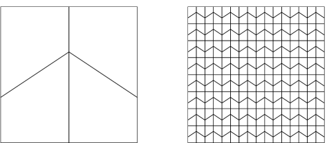
Figure 1. a. A partition of the square into four trapezoids. b. A mesh composed of translated dilates of this partition.

The four quadrilaterals are mutually congruent and affinely related to the specific quadrilateral $K^{\prime}$ defined above. Therefore, by Theorem 4, we can define for each of the four quadrilaterals $K^{\prime\prime}$ shown in Figure 1 an isomorphism $F^{\prime\prime}$ from the unit square so that $V_{F^{\prime\prime}}(K^{\prime\prime})\nsupseteq\mathcal{P}_{r}(K^{\prime\prime})$. If we let $\hat{S}$ be the subspace of $L^{2}(\hat{K})$ consisting of functions which restrict to elements of $V_{F^{\prime\prime}}(K^{\prime\prime})$ on each of the four quadrilaterals $K^{\prime\prime}$, then certainly $\hat{S}$ does not contain $\mathcal{P}_{r}(\hat{K})$, since even its restriction to any one of the quadrilaterals $K^{\prime\prime}$ does not contain $P_{r}(K^{\prime\prime})$.

Next, for $n=1,2,\ldots$ consider the mesh $\mathcal{T}^{\prime}_{h}$ of the unit square $\Omega$ shown in Figure 1b, obtained by first dividing it into a uniform $n\times n$ mesh of subsquares, $n=1/h$, and then dividing each subsquare as in Figure 1a. Then the space of functions $u$ on $\Omega$ whose restrictions on each subsquare $K\in\mathcal{T}_{h}$ satisfy $\hat{u}_{K}(\hat{x})=u(x_{K}+h\hat{x})$ with $\hat{u}_{K}\in\hat{S}$ is precisely the same as the space $V(\mathcal{T}^{\prime}_{h})$ constructed from the initial space $\hat{V}$ and the mesh $\mathcal{T}^{\prime}_{h}$. In view of Theorems 1 and 2 and the fact that $\hat{S}\nsupseteq\mathcal{P}_{r}(\hat{K})$, the estimates (4) and (5) do not hold. In fact, neither of the estimates

$$\inf_{v\in V(\mathcal{T}_{h})}\lVert u-v\rVert_{L^{2}(\Omega)}=o(h^{r}),$$

nor

$$\inf_{v\in V(\mathcal{T}_{h})}\lVert\nabla(u-v)\rVert_{L^{2}(\Omega)}=o(h^{r-1}),$$

holds, even for $u\in\mathcal{P}_{r}(\Omega)$.

While the condition $\hat{V}\supseteq\mathcal{Q}_{r}(\hat{K})$ is necessary for $O(h^{r+1})$ on general quadrilateral meshes, the conditions $\hat{V}\supseteq\mathcal{P}_{r}(\hat{K})$ suffices for meshes of parallelograms. Naturally, the same is true for meshes whose elements are sufficiently close to parallelograms. We conclude this section with a precise statement of this result and a sketch of the proof. If $\hat{V}\supseteq\mathcal{P}_{r}(\hat{K})$ and $K=F(\hat{K})$ with $F\in\operatorname{\mathsf{Bil}}(\hat{K})$, then by standard arguments, as in [1], we get

$$\|v-\pi v\|_{L^{2}(K)}\leq C\|J_{F}\|_{L^{\infty}(\hat{K})}^{1/2}|v\circ F|_{H^{r+1}(\hat{K})},$$

where $J_{F}$ is the Jacobian determinant of $F$. Now, using the formula for the derivative of a composition (as in, e.g., [3, p. 222]), and the fact that $F$ is quadratic, and so its third and higher derivatives vanish, we get that

$$|v\circ F|_{H^{r+1}(\hat{K})}\leq C\|J_{F^{-1}}\|_{L^{\infty}(K)}^{1/2}\|v\|_{H^{r+1}(K)}\sum_{i=0}^{\lfloor(r+1)/2\rfloor}|F|_{W^{1}_{\infty}(\hat{K})}^{r+1-2i}|F|_{W^{2}_{\infty}(\hat{K})}^{i}.$$

Now,

$$\|J_{F}\|_{L^{\infty}(\hat{K})}\leq Ch_{K}^{2},\quad\|J_{F^{-1}}\|_{L^{\infty}(\hat{K})}\leq Ch_{K}^{-2},\quad|F|_{W^{1}_{\infty}(\hat{K})}\leq Ch_{K},$$

where $h_{K}$ is the diameter of $K$ and $C$ depends only on the shape-regularity of $K$. We thus get

$$\|v-\pi v\|_{L^{2}(K)}\leq C\|v\|_{H^{r+1}(K)}\sum_{i}h_{K}^{r+1-2i}|F|_{W^{2}_{\infty}(\hat{K})}^{i}.$$

It follows that if $|F|_{W^{2}_{\infty}(\hat{K})}=O(h_{K}^{2})$, we get the desired estimate

$$\|v-\pi v\|_{L^{2}(K)}\leq Ch_{K}^{r+1}\|v\|_{H^{r+1}(K)}.$$

Following [5], we measure the deviation of a quadrilateral from a parallelogram, by the quantity $\sigma_{K}:=\max(|\pi-\theta_{1}|,|\pi-\theta_{2}|)$, where $\theta_{1}$ is the angle between the outward normals of two opposite sides of $K$ and $\theta_{2}$ is the angle between the outward normals of the other two sides. Thus $0\leq\sigma_{K}<\pi$, with $\sigma_{K}=0$ if and only if $K$ is a parallelogram. As pointed out in [5], $|F|_{W^{2}_{\infty}(\hat{K})}\leq Ch_{K}(h_{K}+\sigma_{K})$. This motivates the definition that a family of quadrilateral meshes is asymptotically parallelogram if $\sigma_{K}=O(h_{K})$, i.e., if $\sigma_{K}/h_{K}$ is uniformly bounded for all the elements in all the meshes. From the foregoing considerations, if the reference space contains $\mathcal{P}_{r}(\hat{K})$ we obtain $O(h^{r+1})$ convergence for asymptotically parallelogram, shape regular meshes.

As a final note, we remark that any polygon can be meshed by an asymptotically parallelogram, shape regular family of meshes with mesh size tending to zero. Indeed, if we begin with any mesh of convex quadrilaterals, and refine it by dividing each quadrilateral in four by connecting the midpoints of the opposite edges, and continue in this fashion, as in the last row of Figure 2, the resulting mesh is asymptotically parallelogram and shape regular.

4. Numerical results

In this section we report on results from a numerical study of the behavior of piecewise continuous mapped biquadratic and serendipity finite elements on quadrilateral meshes (i.e., the finite element spaces are constructed starting from the spaces $Q_{2}(\hat{K})$ and $S_{2}(\hat{K})$ on the reference square, and then imposing continuity). We present the results of two test problems. In both we solve the Dirichlet problem for Poisson’s equation

(7) $$-\Delta u=f\text{ in $\Omega$},\quad u=g\text{ on $\partial\Omega$},$$

where the domain $\Omega$ is the unit square. In the first problem, $f$ and $g$ are taken so that the exact solution is the quartic polynomial

$$u(x,y)=x^{3}+5y^{2}-10y^{3}+y^{4}.$$

Table 1 shows results for both types of elements using meshes from each of the first two mesh sequences shown in Figure 2. The first sequence of meshes consists of uniform square subdivisions of the domain into $n\times n$ subsquares, $n=2,4,8,\ldots$. Meshes in the second sequence are partitions of the domain into $n\times n$ congruent trapezoids, all similar to the trapezoid with vertices $(0,0)$, $(1/2,0)$, $(1/2,2/3)$, and $(0,1/3)$. In Table 1 we report the errors in $L^{2}$ for the finite element solution and its gradient both in absolute terms and as a percentage of the $L^{2}$ norm of the exact solution and its gradient, and we also report the apparent rate of convergence based on consecutive meshes in a sequence. For this test problem, the rates of convergence are very clear: for either mesh sequence the mapped biquadratic elements converge with the expected order $3$ for the solution and $2$ for its gradient. The same is true for the serendipity elements on the square meshes, but, as predicted by the theory given above, for the trapezoidal mesh sequence the order of convergence for the serendipity elements is reduced by $1$ both for the solution and its gradient.

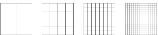
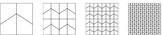
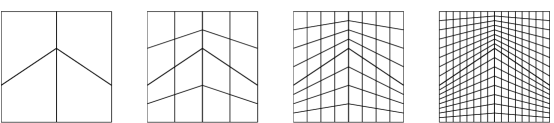
Figure 2. Three sequences of meshes of the unit square: square, trapezoidal, and asymptotically parallelogram. Each is shown for $n=2$ ,$4$, $8$, and $16$.

Table 1. Errors and rates of convergence for the test problem with polynomial solution.

Mapped biquadratic elements
	square meshes						trapezoidal meshes
	$\|u-u_{h}\|_{L^{2}}$			$\|\nabla(u-u_{h})\|_{L^{2}}$			$\|u-u_{h}\|_{L^{2}}$			$\|\nabla(u-u_{h})\|_{L^{2}}$
$n$	err.	%	rate	err.	%	rate	err.	%	rate	err.	%	rate
2	3.5e$-$02	2.877		4.5e$-$01	37.253		4.8e$-$02	3.951		5.9e$-$01	48.576
4	4.4e$-$03	0.360	3.0	1.1e$-$01	9.333	2.0	5.8e$-$03	0.475	3.1	1.5e$-$01	12.082	2.0
8	5.5e$-$04	0.045	3.0	2.8e$-$02	2.329	2.0	7.1e$-$04	0.058	3.0	3.7e$-$02	3.017	2.0
16	6.9e$-$05	0.006	3.0	7.1e$-$03	0.583	2.0	8.7e$-$05	0.007	3.0	9.2e$-$03	0.753	2.0
32	8.6e$-$06	0.001	3.0	1.8e$-$03	0.146	2.0	1.1e$-$05	0.001	3.0	2.3e$-$03	0.188	2.0
64	1.1e$-$06	0.000	3.0	4.4e$-$04	0.036	2.0	1.3e$-$06	0.000	3.0	5.7e$-$04	0.047	2.0
Serendipity elements
	square meshes						trapezoidal meshes
	$\|u-u_{h}\|_{L^{2}}$			$\|\nabla(u-u_{h})\|_{L^{2}}$			$\|u-u_{h}\|_{L^{2}}$			$\|\nabla(u-u_{h})\|_{L^{2}}$
$n$	err.	%	rate	err.	%	rate	err.	%	rate	err.	%	rate
2	3.5e$-$02	2.877		4.5e$-$01	37.252		5.0e$-$02	4.066		6.2e$-$01	51.214
4	4.4e$-$03	0.360	3.0	1.1e$-$01	9.333	2.0	6.7e$-$03	0.548	2.9	1.8e$-$01	14.718	1.8
8	5.5e$-$04	0.045	3.0	2.8e$-$02	2.329	2.0	9.7e$-$04	0.080	2.8	5.9e$-$02	4.836	1.6
16	6.9e$-$05	0.006	3.0	7.1e$-$03	0.583	2.0	1.6e$-$04	0.013	2.6	2.3e$-$02	1.890	1.4
32	8.6e$-$06	0.001	3.0	1.8e$-$03	0.146	2.0	3.3e$-$05	0.003	2.3	1.0e$-$02	0.842	1.2
64	1.1e$-$06	0.000	3.0	4.4e$-$04	0.036	2.0	7.4e$-$06	0.001	2.1	4.9e$-$03	0.401	1.1

As a second test example we again solved the Dirichlet problem (7), but this time choosing the data so that the solution is the sharply peaked function

$$u(x,y)=\exp\bigl{(}-100[(x-1/4)^{2}+(y-1/3)^{2}]\bigr{)}.$$

As seen in Table 2, in this case the loss of convergence order for the serendipity elements on the trapezoidal mesh is not nearly as clear. Some loss is evident, but apparently very fine meshes (and very high precision computation) would be required to see the final asymptotic orders.

Table 2. Errors and rates of convergence for the test problem with exponential solution.

Mapped biquadratic elements
	square meshes						trapezoidal meshes
	$\|u-u_{h}\|_{L^{2}}$			$\|\nabla(u-u_{h})\|_{L^{2}}$			$\|u-u_{h}\|_{L^{2}}$			$\|\nabla(u-u_{h})\|_{L^{2}}$
$n$	err.	%	rate	err.	%	rate	err.	%	rate	err.	%	rate
2	2.8e$-$01	224.000		3.0e$+$00	169.630		2.6e$-$01	204.800		2.8e$+$00	159.208
4	1.2e$-$01	93.600	1.3	1.5e$+$00	87.322	1.0	2.1e$-$01	169.600	0.3	1.8e$+$00	99.305	0.7
8	1.7e$-$02	13.520	2.8	4.6e$-$01	25.809	1.8	2.3e$-$02	18.160	3.2	5.9e$-$01	33.185	1.6
16	1.1e$-$03	0.920	3.9	1.0e$-$01	5.860	2.1	1.3e$-$03	1.048	4.1	1.2e$-$01	6.819	2.3
32	1.3e$-$04	0.101	3.2	2.5e$-$02	1.424	2.0	1.5e$-$04	0.124	3.1	3.2e$-$02	1.794	1.9
64	1.5e$-$05	0.012	3.1	6.3e$-$03	0.354	2.0	1.9e$-$05	0.015	3.0	7.9e$-$03	0.448	2.0
128	1.9e$-$06	0.002	3.0	1.6e$-$03	0.088	2.0	2.4e$-$06	0.002	3.0	2.0e$-$03	0.112	2.0
Serendipity elements
	square meshes						trapezoidal meshes
	$\|u-u_{h}\|_{L^{2}}$			$\|\nabla(u-u_{h})\|_{L^{2}}$			$\|u-u_{h}\|_{L^{2}}$			$\|\nabla(u-u_{h})\|_{L^{2}}$
$n$	err.	%	rate	err.	%	rate	err.	%	rate	err.	%	rate
2	2.0e$-$01	159.200		2.4e$+$00	133.372		2.1e$-$01	169.600		2.3e$+$00	130.340
4	1.2e$-$01	92.000	0.8	1.4e$+$00	80.531	0.7	2.1e$-$01	168.000	0.0	1.7e$+$00	93.819	0.5
8	1.7e$-$02	13.520	2.8	4.6e$-$01	26.293	1.6	2.4e$-$02	18.880	3.2	6.1e$-$01	34.564	1.4
16	1.1e$-$03	0.920	3.9	1.1e$-$01	5.948	2.1	1.5e$-$03	1.208	4.0	1.4e$-$01	7.737	2.2
32	1.3e$-$04	0.101	3.2	2.5e$-$02	1.432	2.1	2.0e$-$04	0.162	2.9	3.8e$-$02	2.156	1.8
64	1.5e$-$05	0.012	3.1	6.3e$-$03	0.354	2.0	2.7e$-$05	0.022	2.9	1.1e$-$02	0.597	1.9
128	1.9e$-$06	0.002	3.0	1.6e$-$03	0.088	2.0	3.7e$-$06	0.003	2.9	3.4e$-$03	0.191	1.6

Finally we return to the first test problem, and consider the behavior of the serendipity elements on the third mesh sequence shown in Figure 2. This mesh sequence begins with the same mesh of four quadrilaterals as in previous case, and continues with systematic refinement as described at the end of the last section, and so is asymptotically parallelogram. Therefore, as explained there, the rate of convergence for serendipity elements is the same as for affine meshes. This is clearly illustrated in Table 3.

Table 3. Errors and rates of convergence for the test problem with polynomial solution using serendipity elements on asympotically affine meshes.

	$\|u-u_{h}\|_{L^{2}}$			$\|\nabla(u-u_{h})\|_{L^{2}}$
$n$	err.	%	rate	err.	%	rate
2	5.0e$-$02	4.066		6.2e$-$01	51.214
4	6.2e$-$03	0.510	3.0	1.5e$-$01	12.109	2.1
8	7.6e$-$04	0.062	3.0	3.6e$-$02	2.948	2.0
16	9.4e$-$05	0.008	3.0	9.0e$-$03	0.735	2.0
32	1.2e$-$05	0.001	3.0	2.2e$-$03	0.183	2.0
64	1.5e$-$06	0.000	3.0	5.6e$-$04	0.046	2.0
128	1.9e$-$07	0.000	3.0	1.4e$-$04	0.012	2.0

While the asymptotic rates predicted by the theory are confirmed in these examples, it is worth noting that in absolute terms the effect of the degraded convergence rate is not very pronounced. For the first example, on a moderately fine mesh of $16\times 16$ trapezoids, the solution error with serendipity elements exceeds that of mapped biquadratic elements by a factor of about 2, and the gradient error by a factor of 2.5. Even on the finest mesh shown, with $64\times 64$ elements, the factors are only about 5.5 and 8.5, respectively. Of course, if we were to compute on finer and finer meshes with sufficiently high precision, these factors would tend to infinity. Indeed, on any quadrilateral mesh which contains a non-parallelogram element, the analogous factors can be made as large as desired by choosing a problem in which the exact solution is sufficiently close to—or even equal to—a quadratic function, which the mapped biquadratic elements capture exactly, while the serendipity elements do not (such a quadratic function always exists). However, it is not unusual that the serendipity elements perform almost as well as the mapped biquadratic elements for reasonable, and even for quite small, levels of error. This, together with their optimal convergence on asymptotically parallelogram meshes, provides an explanation of why the lower rates of convergence have not been widely noted.

References

- [1] P. G. Ciarlet, The finite element method for elliptic problems, North-Holland, Amsterdam, 1978.
- [2] P. G. Ciarlet and P.-A. Raviart, Interpolation theory over curved elements with applications to fiite element methods, Comput. Methods Appl. Mech. Engrg. 1 (1972), 217–249.
- [3] H. Federer, Geometric measure theory, Springer-Verlag, New York, 1969.
- [4] V. Girault and P.-A. Raviart, Finite element methods for Navier-Stokes equations, Springer-Verlag, New York, 1986.
- [5] R. Rannacher and S. Turek, Simple nonconforming quadrilateral stokes element, Numer. Meth. Part. Diff. Equations 8 (1992), 97–111.
- [6] P. Sharpov and Y. Iordanov, Numerical solution of Stokes equations with pressure and filtration boundary conditions, J. Comp. Phys. 112 (1994), 12–23.
- [7] O. C. Zienkiewicz and R. L. Taylor, The finite element method, fourth edition, volume 1: Basic formulation and linear problems, McGraw-Hill, London, 1989.