Enhancement of the inverse-cascade of energy in the two-dimensional averaged Euler equations

Abstract

For a particular choice of the smoothing kernel, it is shown that the system of partial differential equations governing the vortex-blob method corresponds to the averaged Euler equations. These latter equations have recently been derived by averaging the Euler equations over Lagrangian fluctuations of length scale $\alpha$, and the same system is also encountered in the description of inviscid and incompressible flow of second-grade polymeric (non-Newtonian) fluids. While previous studies of this system have noted the suppression of nonlinear interaction between modes smaller than $\alpha$, we show that the modification of the nonlinear advection term also acts to enhance the inverse-cascade of energy in two-dimensional turbulence and thereby affects scales of motion larger than $\alpha$ as well. This latter effect is reminiscent of the drag-reduction that occurs in a turbulent flow when a dilute polymer is added.

The two-dimensional incompressible, Euler equations are

$$\partial_{t}\omega+\mbox{\boldmath$\nabla$}\cdot\left(\text{u}\,\omega\right)=0,\quad\mbox{\boldmath$\nabla$}\cdot\text{u}=0,\quad\omega(t=0)=\omega_{0},$$ (1)

where $\omega=\mbox{\boldmath$\nabla$}\times\text{u}$ is the vorticity, u is the spatial velocity vector field, $t$ denotes time, and all the dependent variables depend on $t$ and $\text{x}=(x_{1},x_{2})$, the Cartesian coordinates in the plane. An inversion of the vorticity-velocity relation yields $\text{u}=\int\text{K}(\text{x},\text{y})\omega(\text{y})d\text{y}$, where $\text{K}=\mbox{\boldmath$\nabla$}^{\perp}G$, $G$ is the solution of $-\triangle G=\delta$, and $\mbox{\boldmath$\nabla$}^{\perp}=(-\partial_{x_{1}},\partial_{x_{2}})$.For fluid motion over the entire plane, $\text{K}(\text{x},\text{y})=(2\pi)^{-1}\mbox{\boldmath$\nabla$}^{\perp}\log|\text{x}-\text{y}|$. Let $\mbox{\boldmath$\eta$}_{t}$ denote the flow of $\text{u}_{t}=\text{u}(t,\cdot)$, so that $d\mbox{\boldmath$\eta$}_{t}/dt=\text{u}_{t}(\mbox{\boldmath$\eta$}(t))$. Because $\text{u}_{t}$ is divergence-free, the flow map $\mbox{\boldmath$\eta$}_{t}$ is an area-preserving transformation for each $t$. It follows that

$$\frac{d\mbox{\boldmath$\eta$}_{t}}{dt} =\int\text{K}(\mbox{\boldmath$\eta$}_{t}(\text{x}),\mbox{\boldmath$\eta$}_{t}(\text{y}))\omega(\mbox{\boldmath$\eta$}_{t}(\text{y}))d\text{y}$$ (2)

$$=\int\text{K}(\mbox{\boldmath$\eta$}_{t}(\text{x}),\mbox{\boldmath$\eta$}_{t}(\text{y}))\omega_{0}(\text{y})d\text{y},$$ (3)

where the last equality is a consequence of the pointwise conservation of vorticity along Lagrangian trajectories, $\omega(\mbox{\boldmath$\eta$}_{t}(\text{x}))=\omega_{0}(\text{x})$. Thus, the initial vorticity field completely determines the fluid motion. Choosing the initial vorticity to be a sum of $N$ point vortices $\delta_{i}$ positioned at the points $\text{x}_{i}$ in the plane with circulations $\Gamma_{i}$, $\omega_{0}=\sum_{i=1}^{N}\Gamma_{i}\delta_{i}$, equation (2) produces the classical point-vortex approximation to (1). This approximation is known to be highly unstable, as finite-time collapse of vortex centers may occur [7].

Chorin’s vortex blob method [3] alleviates the instability of the point-vortex scheme by smoothing each delta function $\delta_{i}$ with a vortex blob $\chi$, a function that decays at infinity, and whose mass is mostly supported in a disc of diameter $\alpha$. Thus, instead of using the integral kernel $\text{K}(\text{x},\text{y})$, one uses the smoother kernel $\text{K}^{\alpha}=\mbox{\boldmath$\nabla$}^{\perp}G^{\alpha}$ where $G^{\alpha}$ is the solution of $-\triangle G^{\alpha}=\chi.$ The vortex-blob method then evolves the point-vortex initial data, which we shall now call $q_{0}$, by the ordinary differential equation

$$\frac{d\mbox{\boldmath$\eta$}_{t}^{\alpha}}{dt}=\int\text{K}^{\alpha}(\mbox{\boldmath$\eta$}_{t}^{\alpha}(\text{x}),\mbox{\boldmath$\eta$}_{t}^{\alpha}(\text{y}))q_{0}(\text{y})d\text{y}.$$ (4)

Henceforth, to keep the notation concise, we will drop the superscript $\alpha$ when there is no ambiguity.

When the vortex-blob $G^{\alpha}$ is the modified Bessel function of the second kind $K_{0}$, it is the fundamental solution of the operator $(1-\alpha^{2}\triangle)$ in the plane, and the vorticity $q$ is related to the smoothed velocity vector field u by $q=(1-\alpha^{2}\triangle)\mbox{\boldmath$\nabla$}\times\text{u}$. Thus, Chorin’s vortex method for this choice of smoothing is given by the partial differential equation

$$\partial_{t}q+\mbox{\boldmath$\nabla$}\cdot\left(\text{u}\,q\right)=0,\quad\mbox{\boldmath$\nabla$}\cdot\text{u}=0,\quad q(t=0)=q_{0},$$ (5)

The system of equations (5) is also known as the two-dimensional isotropic averaged Euler equations, and are derived by averaging over Lagrangian fluctuations of order $\alpha$ about the macroscopic flow field [5, 14, 8]. When the constant $\alpha>0$ is interpreted as a material parameter which measures the elastic response of the fluid due to polymerization instead of as a spatial length scale, then (5) are also exactly the equations that govern the inviscid flow of a second-grade non-Newtonian fluid [11]. According to Noll’s theory of simple materials, (5) are obtained from the unique constitutive law that satisfies material frame-indifference and observer objectivity. Consequently, the vortex method with the Bessel function $K_{0}$ smoothing naturally inherits these characteristics [13].

We find the connections between averaging Euler equations over Lagrangian fluctuations, a constitutive theory for polymeric fluids, and a classical numerical algorithm to be quite intriguing and suspect that these equations will be important from a modeling standpoint. However, most previous studies of the averaged Euler equations have been of a mathematical nature, and we are aware of only a few cases where this system has been used as a (dynamic) modeling tool: Chen et al. [2] used a viscous version of the three-dimensional averaged Euler equations to simulate isotropic turbulence and found that they could reproduce large-scale features without fully resolving the flow. Nadiga [9] considered the inviscid two-dimensional form of the averaged Euler equations and demonstrated that for suitably chosen values of $\alpha$, the large-scale spectral-scalings of the Euler equations could be preserved while achieving a faster spectral decay at the smaller scales. Finally, Nadiga & Margolin [10] used an extension of the two-dimensional averaged Euler equations in a geophysical context to model the effects of mesoscale eddies on mean flow.

Before we go on to consider numerical simulation of the averaged Euler system, we wish to point out that there is also a beautiful geometric structure to (5) which follows the framework developed by Arnold [1] and Ebin and Marsden [4]. While the details of this particular issue are far outside the scope of this article, it is, nevertheless, worthwhile to state the result. Arnold showed that the appropriate configuration space for a perfect incompressible fluid is the group of all area preserving diffeomorphisms of the fluid container, and that solutions of the Euler equations are geodesics on this group with respect to a certain kinetic energy metric, characterized by the inner-product $\int\left(\text{u}\cdot\text{v}\right)\,d\text{x}$ for two divergence-free vector fields u and v. The system (5) also has this geometric property, but now the metric is instead characterized by $\int\left(\text{u}\cdot\text{v}+2\alpha^{2}\text{Def}(\text{u})\cdot\text{Def}(\text{v})\right)d\text{x},$ where $\text{Def}(\text{u})$ is the rate of deformation tensor $(\mbox{\boldmath$\nabla$}\text{u}+(\mbox{\boldmath$\nabla$}\text{u})^{T})/2$ [15]. Equations (5) thus preserve the Hamiltonian structure of the Euler equations. In particular, vorticity remains pointwise conserved by the smooth Lagrangian flow $\mbox{\boldmath$\eta$}_{t}^{\alpha}$ so that $q(\mbox{\boldmath$\eta$}_{t}^{\alpha}(\text{x}))=q_{0}(\text{x}),$ the vorticity momenta $\int q^{p}d\text{x}$ are conserved, and so the Kelvin circulation theorem remains intact [5] as well.

Since, in each of the three different scenarios—averaged Euler, vortex-blob method, and inviscid second-grade fluid—the essential modification of the original equations is a change of the advective nonlinearity of fluid dynamics, we will now consider forced-dissipative simulations of the system (5) to demonstrate the effect of such an inviscid modification. If we use a vorticity-stream function formulation, the evolution of both the Euler and averaged Euler sytems can be represented by

$$\frac{\partial\omega}{\partial t}+(1-\alpha^{2}\triangle)^{-1}J[\psi,(1-\alpha^{2}\triangle)\omega]=F+D;\quad$$ (6)

where $\omega=\triangle\psi$, $J$ is the Jacobian, $F$ the forcing, and $D$ the dissipation. (The Euler system corresponds to $\alpha=0$.) Our numerical scheme consists of a fully dealiased pseudospectral spatial discretization and a (nominally) fifth-order, adaptive timestep, embedded Runge-Kutta Cash-Karp temporal discretization of (6) (see Nadiga [9] for details). With such a scheme, among the infinity of inviscid ($F=D=0$) conserved quantities for (6), the only two conservation properties that survive are those for the kinetic energy $E_{H^{1}}$ and enstrophy $Z_{H^{2}}$ given respectively by

$$E_{H^{1}} = \frac{1}{2}\int\left(|\text{u}|^{2}+\alpha^{2}|\mbox{\boldmath$\nabla$}\text{u}|^{2}\right)d\text{x}\;\left(=\|\text{u}\|_{H^{1}}^{2}\right),$$ (7)

$$Z_{H^{2}} = \frac{1}{2}\int\left[\left(1-\alpha^{2}\triangle\right)\omega\right]^{2}d\text{x}\;\left(=\|\omega\|^{2}_{H^{2}}\right).$$ (8)

In the forced-dissipative runs to be considered, the forcing $F$ is achieved by keeping the amplitudes of modes with wavenumbers in the small wavenumber band $10\leq k<10.001$ constant in time. The dissipation, $D$, is a combination of a fourth order hyperviscous operator and a large-scale friction term: $D=\delta\psi-\left(-\nu\triangle\right)^{4}\omega$, as has been used in numerous previous studies of two-dimensional turbulence. The form and value of the forcing and dissipation are held exactly the same for all the runs to be presented, irrespective of the resolution and the value of $\alpha$.

On the one hand, it could be argued that since the energy and enstrophy that are conserved (in an unforced-inviscid setting) are $E_{H^{1}}$ and $Z_{H^{2}}$ respectively, it is their dynamics which is of primary importance. On the other, it could be argued that in the context of (6), the interest in small scales is only in so much as it affects the larger scales and to that extent $\alpha$ has no primary significance and that it is really the large scale components of energy and enstrophy in (7) that are of primary interest. While both these points of view are reasonable, in this short article, we proceed with the latter and concern ourselves with the dynamics of the usual kinetic energy and usual enstrophy as given by

$$E=\frac{1}{2}\int|\text{u}|^{2}d\text{x},\quad Z=\frac{1}{2}\int\omega^{2}d\text{x}.$$ (9)

Fig. 1 shows the evolution of the kinetic energy $E$ with time for four different values of $k_{\alpha}$. For these computations, 512 physical grid points were used in each direction, resulting in, after accounting for dealiasing, a maximum, circularly-symmetric wavenumber, $k_{max}$, of 170. The four runs correspond to $k_{\alpha}$ of $\infty$ (dissipative Euler) and 42, 21, and 14. This figure shows that for identical forcing and dissipation, the tendency with increasing $\alpha$ (equivalently decreasing $k_{\alpha}$) is to achieve an overall balance which makes the flow less viscous.

While the kinetic energy of the runs with different $\alpha$ shows a definite trend (increasing with increasing $\alpha$), such is not the case with the enstrophy shown for the same four cases in the inset of Fig. 1. Here interestingly, all the runs with nonzero $\alpha$ seem to display approximately the same level of enstrophy which is lower than for $k_{\alpha}=0$. This indicates:

• That the small-scale behavior is quite different when $\alpha=0$ and when $\alpha$ is nonzero (as noted in previous studies [5, 2, 9]), but that this difference is not sensitively dependent on the value of $\alpha$ for the interesting range of values of $\alpha$.

• That the more significant change with $\alpha$ is the behavior of the large scales.

Therefore, to further examine the nature of this (reduced-viscous) behavior of the large scales, we examine the energy-wavenumber spectra in Fig. 2. Here, the average of the one dimensional energy spectrum $E(k)$ between times 5 and 20 is plotted against the scalar wavenumber $k$. Figure 2 shows that the reduced-viscous behavior for increasing $\alpha$ is achieved by systematically increasing the energy in modes larger in scale than the forcing scale and decreasing the energy in modes smaller in scale compared to the forcing scale.

The larger energy content in the larger scales implies an enhancement of the inverse cascade of energy of two-dimensional turbulence by the nonlinear-dispersive modification of the advective nonlinearity when $\alpha>0$ in (6). So also, the decreased energy content in the smaller scales is attributable to the same nonlinear-dispersive modification. In the following, we give a simple dimensional argument to explain the observed behavior. For this, consider the governing equations in the form (5). In close analogy with the classical picture for the inertial ranges of two-dimensional dissipative Euler equations [6], a Kolmogorov-like cascade picture for (5) shows that the inertial range consists of two subranges, the enstrophy cascade subrange where there is a down-scale cascade of the $Z_{H^{2}}$ enstrophy defined in (7), and the energy cascade subrange where there is an up-scale cascade of the $E_{H^{1}}$ energy defined in (7). $E_{H^{1}}$ and $Z_{H^{2}}$ are the relevant energy and enstrophies since these are the ones which are conserved in an inviscid and unforced case.

If we assume that the wavenumber $k_{\alpha}$ only appears in the Helmholtz operator, as it does in the governing equations, then

• In the enstrophy cascade subrange,

  $$E(k)\sim\beta_{H^{2}}^{a}k^{b},$$ (10)

  where $\beta_{H^{2}}$ is the rate of dissipation of $Z_{H^{2}}$ enstrophy, and $a$ and $b$ are exponents to be determined by dimensional analysis. If $L$ and $T$ are characteristic length and time scales in the enstrophy cascade subrange, (10) implies

  $$L^{3}T^{-2}=T^{-3a}\left(1+\alpha^{2}L^{-2}\right)^{2a}L^{-b},$$

  from which $a=2/3$. However, even in the enstrophy cascade subrange, the value of $b$ depends on the the ratio $\alpha/L$. For $\alpha\ll L$, of course, $b=-3$, and the classical [6] $E(k)\sim k^{-3}$ is recovered; when $\alpha\gg L$, $E(k)\sim k^{-\frac{17}{3}}$. Finally, when $\alpha$ is comparable to $L$, it is easy to see that $E(k)$ decays faster than for Euler, but slower than $k^{-\frac{17}{3}}$ (as may be seen in Fig. 2).

• In the energy cascade subrange,

  $$E(k)\sim\epsilon_{H^{1}}^{a}k^{b},$$ (11)

  where $\epsilon_{H^{1}}$ is the rate of dissipation of $E_{H^{1}}$ energy, and $a$ and $b$ are exponents to be determined by dimensional analysis. If $L$ and $T$ are characteristic length and time scales, now, in the energy cascade subrange, (11) implies

  $$L^{3}T^{-2}=T^{-3a}\left(1+\alpha^{2}L^{-2}\right)^{a}L^{2a-b},$$

  from which $a=2/3$. Again, even in the energy cascade subrange, the value of $b$ depends on the the ratio $\alpha/L$. For $\alpha\ll L$, of course, $b=-\frac{5}{3}$, and the classical [6] $E(k)\sim k^{-\frac{5}{3}}$ is recovered; when $\alpha\gg L$, $E(k)\sim k^{-3}$. When $\alpha$ is comparable to $L$, it is easy to see that the inverse cascade of energy is enhanced, that is $E(k)$ increases with decreasing $k$ faster than $k^{-\frac{5}{3}}$ (Euler) but slower than $k^{-3}$.

While the effects of the enhancement of the inverse cascade of energy is clear in Fig. 2, we defer the verification of the asymptotic values of the exponent $b$ to later studies when we can afford much larger simulations with a good dynamic range in each of the inertial subranges.

The steeper fall-off of the energy spectrum with $k$ in the enstrophy cascade range of wavenumbers when $\alpha>0$, compared to Euler may, at first, suggest that a coarser resolution may be sufficient to resolve the flow when $\alpha>0$ (for the same forcing and dissipation). However, this is not the case, as should be clear from Fig. 3. In this figure, the spectra of the cases previously discussed is replotted together with the corresponding spectra when the resolution is reduced by a quarter ($k_{max}=128$) and a half ($k_{max}=85$). (The spectra for the different values of $\alpha$ are offset to improve clarity.) The degree of non-resolution of the flow due to the reduced resolution is indicated by the deviation of that spectrum from that for the fully resolved case. With a 25% reduction in resolution, the flows are almost resolved for all values of $\alpha$, while with a 50% reduction, the flows are not fully resolved anymore. Importantly, the degree of non-resolution is independent of $\alpha$ to the lowest order.

Besides their use in describing mean motion, the averaged Euler equations have arisen independently in at least two other contexts—second grade polymeric fluids and vortex blob methods. In this note, we make two observations that are likely to be of fundamental importance in understanding the relevance of these models in describing more realistic flows: While it has been previously noted that with these equations, nonlinear interactions at scales small compared to $\alpha$ are suppressed, we have shown here that the modification of the nonlinear advection term in these equations also leads to an enhancement of the inverse cascade of energy in two dimentions—a characteristic feature of two-dimensional turbulence. This in turn implies (1) an overall reduced-viscous behavior and (2) a significant modification of the dynamics of scales larger than $\alpha$, both reminiscent of the phenomenon of drag reduction in a turbulent flow when a dilute polymer is added (e.g., see [12] and references therein). Furthermore, we point out that the limiting of the energy spectrum at small scales due to $\alpha$ does not, in itself, allow the flow to be resolved on a coarser grid.

The latter notwithstanding, we remark that the averaged Euler equations are useful in better understanding the limit of inviscid fluid flow, since the averaged Euler equations with viscosity, unlike the Euler equations, converge regularly to the solutions of the inviscid system[15]. That is, for an arbitrary but fixed time interval, we can choose $\alpha$ small enough so that the solution of the averaged Euler equations are uniformly within any a priori chosen error of the Euler equations[13] and then consider the zero viscosity limit of the viscous, averaged Euler equations.

Finally, we note that as a theoretical model of fluid turbulence, the averaged Euler equations in two dimensions possess other remarkable features. For example, for any initial condition and fixed time interval, one may choose the number of modes $k_{max}$ large enough so as to be arbitrarily close to the exact solution of the averaged Euler equations without the addition of viscosity. For such large $k_{max}$, and in simulations of unforced decaying turbulence, the averaged Euler equations exhibit a fundametal feature of two-dimensional turbulence: a sharp decrease in enstrophy $Z$ during the first few large eddy turnover times. This is extremely interesting, because, while it is necessary to add viscosity to the Euler equations to obtain similar behavior, the averaged Euler equations can reproduce this behavior while exactly conserving an energy. We shall report further on such inviscid simulations in future publications.

The authors thank Jerry Marsden, and David Montgomery for extensive discussions on a variety of issues related to this article. BTN was supported by the Climate Change Prediction Program of the Department of Energy, and SS was partially supported by NSF-KDI grant ATM-98-73133 and the Alfred P. Sloan Research Fellowship.

FIG. 1.: The evolution of kinetic energy E with time for $k_{\alpha}=\infty$ (solid line), $k_{\alpha}=42$ (dotted line), $k_{\alpha}=21$ (dashed line), and $k_{\alpha}=14$ (dot-dashed line). An increase in $\alpha$, for identical forcing and dissipation, results in an overall reduced viscous behavior. In the inset is shown the evolution of enstrophy Z for the same time interval and for the same four values of $\alpha$ and with the same line types as for kinetic energy. While there is a significant difference between zero and non-zero $\alpha$ cases, the dependence on the actual value of $\alpha$ itself is rather weak.

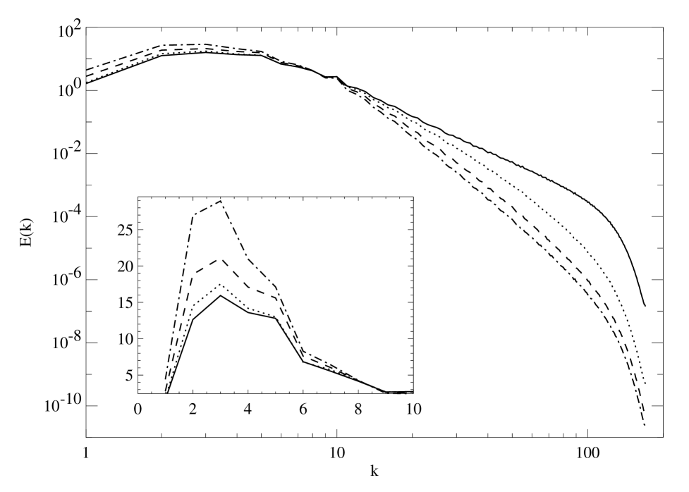
FIG. 2.: Stationary wavenumber-energy spectra (log-log scale) for the forced-dissipative simulations of the averaged Euler equations with zero and nonzero $\alpha$. $k_{\alpha}=\infty$ (solid line), $k_{\alpha}=42$ (dotted line), $k_{\alpha}=21$ (dashed line), and $k_{\alpha}=14$ (dot-dashed line). The insert shows the same plot with a linear-linear scale for the first ten wavenumbers. The enhanced inverse cascade of energy and the suppressed energy level at smaller scales with increasing $\alpha$ is evident.

FIG. 3.: The spectra for the four cases in Fig. 2 are replotted along with the spectra for the same four cases with resolution reduced by 25% and 50% in each direction. The sets of spectra for each $\alpha$ are offset by a decade each to improve clarity. The degree of non-resolution of the flow with the reduced resolution is indicated by the difference between that spectrum and the spectrum for the fully resolved case. With a 25% reduction in resolution, the flows are almost resolved, while with a 50% reduction, the flows are not fully resolved anymore. The degree of non-resolution is independent of $\alpha$ to the lowest order.

REFERENCES

- [1] V.I. Arnold, Sur la geometrie differentielle des groupes de Lie de dimension infinie et ses applications a l’hydrodynamique des fluids parfaits, Ann. Inst. Grenoble, 16, (1966), 319–361.
- [2] S. Chen, D.D. Holm, L. Margolin, and R. Zhang, Direct numerical simulations of the Navier-Stokes alpha model, (1999), preprint.
- [3] A. Chorin, Numerical study of slightly viscous flow, J. Fluid Mech. 57 (1973), 785–796.
- [4] D. Ebin and J. Marsden, Groups of diffeomorphisms and the motion of an incompressible fluid, Ann. of Math., 92, (1970), 102–163.
- [5] D.D. Holm, J.E. Marsden, and T.S. Ratiu, Euler-Poincaré equations and semidirect products with applications to continuum theories, Adv. in Math. 137 (1998), 1–81.
- [6] R.H. Kraichnan, Inertial ranges in two-dimensional turbulence, Phys. Fluids, 10, (1967), 1417–1423.
- [7] C. Marchioro and M. Pulvirenti, Hydrodynamics in two dimensions and vortex theory, Commun. Math. Phys. 84 (1982), 483–503.
- [8] J.E. Marsden and S. Shkoller, The nonisotropic averaged Euler equations, preprint.
- [9] B.T. Nadiga, Scaling properties of an inviscid mean-motion fluid model, J. Stat. Phys, 98 (2000), 935–948.
- [10] B.T. Nadiga and L.G. Margolin, Dispersive eddy parameterization in a barotropic ocean model, submitted to J. Phys. Ocean.
- [11] W. Noll and C. Truesdell, The nonlinear field theories of Mechanics, Springer-Verlag, Berlin, (1965).
- [12] T. Odijk, Polymer-induced vortex modification in decaying two-dimensional turbulence, Physica A, 258 (1998), 329–340.
- [13] M. Oliver and S. Shkoller, The vortex blob method as a second-grade fluid, preprint.
- [14] S. Shkoller, Geometry and curvature of diffeomorphism groups with metric and mean hydrodynamics, J. Funct. Anal. 160 (1998), 337–365.
-
[15]
S. Shkoller, On incompressible
averaged Lagrangian hydrodynamics, (2000), E-print math.AP/9908109,
http://xyz.lanl.gov/abs/math.AP/9908109.