The scaling limit of the incipient infinite cluster
in high-dimensional percolation.
II. Integrated super-Brownian excursion

Abstract

For independent nearest-neighbour bond percolation on ${{{\mathbb{Z}}}^{d}}$ with $d\gg 6$, we prove that the incipient infinite cluster’s two-point function and three-point function converge to those of integrated super-Brownian excursion (ISE) in the scaling limit. The proof is based on an extension of the new expansion for percolation derived in a previous paper, and involves treating the magnetic field as a complex variable. A special case of our result for the two-point function implies that the probability that the cluster of the origin consists of $n$ sites, at the critical point, is given by a multiple of $n^{-3/2}$, plus an error term of order $n^{-3/2-\epsilon}$ with $\epsilon>0$. This is a strong statement that the critical exponent $\delta$ is given by $\delta=2$.

1 Introduction

1.1 The incipient infinite cluster

We consider independent nearest-neighbour bond percolation on ${{{\mathbb{Z}}}^{d}}$. For $x=(x_{1},\ldots,x_{d})\in{{{\mathbb{Z}}}^{d}}$, we write $\|x\|_{1}=\sum_{j=1}^{d}|x_{j}|$. A nearest-neighbour bond is a pair $\{x,y\}$ of sites in ${{{\mathbb{Z}}}^{d}}$ with $\|x-y\|_{1}=1$. To each bond, we associate an independent Bernoulli random variable $n_{\{x,y\}}$, which takes the value 1 with probability $p$, and the value 0 with probability $1-p$. A bond $\{x,y\}$ is said to be occupied if $n_{\{x,y\}}=1$, and vacant if $n_{\{x,y\}}=0$. We say that sites $u,v\in{{{\mathbb{Z}}}^{d}}$ are connected if there is a lattice path from $u$ to $v$ consisting of occupied bonds. In this system, a phase transition occurs, for $d\geq 2$, in the sense that there is a critical value $p_{c}=p_{c}(d)\in(0,1)$, such that for $p<p_{c}$ there is almost surely no infinite connected cluster of occupied bonds, whereas for $p>p_{c}$ there is almost surely a unique infinite connected cluster of occupied bonds (percolation occurs).

It is widely believed that there is no infinite cluster when $p=p_{c}$, but, more than four decades after the mathematical study of percolation was initiated by Broadbent and Hammersley [13], and after considerable study [22, 23, 31, 32], there is still no general proof that this is the case. The absence of an infinite cluster at $p_{c}$ has been proved only for $d=2$ (see [22] and references therein) and, in high dimensions, for $d\geq 19$, and for $d>6$ for sufficiently “spread-out” models having long finite range [6, 25, 27, 38]. We focus in this paper on the high-dimensional case, where the absence of percolation at $p_{c}$ has been established. This presents a picture where at $p_{c}$ there are extensive connections present, on all length scales, but no infinite cluster. However, the slightest increase in $p$ will lead to the formation of an infinite cluster. This inchoate state of affairs at $p_{c}$ is often represented by an appeal to the notion of the “incipient infinite cluster.”

The incipient infinite cluster is a concept admitting various interpretations. A construction of the incipient infinite cluster as an infinite cluster in the 2-dimensional lattice ${\mathbb{Z}}^{2}$ has been carried out by Kesten [33], and, for an inhomogeneous 2-dimensional model, by Chayes, Chayes and Durrett [14]. Such constructions are necessarily singular with respect to the original percolation model, which has no infinite cluster at $p_{c}$. Our point of view is to regard the incipient infinite cluster as a cluster in ${{{\mathbb{R}}}^{d}}$ arising in the scaling limit. More precisely, at $p_{c}$ we condition the size of the cluster of the origin to be $n$, scale space by $n^{-1/4}$ (for $d>6$), and examine the cluster in the limit $n\rightarrow\infty$.

In this paper, we obtain strong evidence for our conjecture that this scaling limit is integrated super-Brownian excursion (ISE) for $d>6$. Our conjecture has been discussed in [29] (see also [18, 41]). ISE can be regarded as the law of a random probability measure on ${{{\mathbb{R}}}^{d}}$, which is almost surely supported on a compact subset of ${{{\mathbb{R}}}^{d}}$. On the scale of the lattice, this compact set corresponds to an infinite cluster, and we therefore regard the limiting object as the scaling limit of the incipient infinite cluster.

In addition to providing the law of a random probability measure on ${{{\mathbb{R}}}^{d}}$, ISE contains more detailed information including the structure of all paths joining pairs of points in the cluster. This is consistent with the interesting recent approach of [2, 3, 4, 5] defining the scaling limit in terms of a collection of continuous paths. In their work, the continuous paths correspond to the occupied paths within all clusters within a large box. Another approach to the incipient infinite cluster is to study the largest clusters present within a large lattice box without taking a scaling limit, as in the work of [3, 12]. In constrast, our focus here is on a single percolation cluster, rather than on many clusters.

In general dimensions, the appropriate spatial scaling of the lattice is presumably $n^{-1/D_{H}}$, where $D_{H}$ is the Hausdorff dimension of the incipient infinite cluster. We will scale space by $n^{-1/4}$ in high dimensions, consistent with the belief that the Hausdorff dimension of the incipient infinite cluster is 4 for $d>6$. The upper critical dimension 6 was identified twenty-five years ago by Toulouse [43] as the dimension above which the behaviour of percolation models near $p_{c}$ should no longer exhibit the dimension-dependence typical of lower dimensions, adopting instead the behaviour associated with percolation on trees.

ISE is defined by conditioning super-Brownian motion to have total mass 1. Super-Brownian motion is a basic example in the theory of superprocesses, modelling a branching Brownian motion in which branching occurs on all (arbitrarily short) length scales. Discussion of ISE can be found in [8, 11, 17, 35, 36]. ISE is almost surely supported on a set of Hausdorff dimension $4$, for dimensions $d\geq 4$, consistent with $D_{H}=4$ for $d>6$.

Our results concern scaling limits of the two-point and three-point functions, at the critical point. Fix $p=p_{c}$ and $x,y\in{{{\mathbb{R}}}^{d}}$. We prove that in sufficiently high dimensions, the probability that a site $\lfloor xn^{1/4}\rfloor\in{{{\mathbb{Z}}}^{d}}$ is connected to the origin, conditional on the cluster size being $n$, corresponds, in the scaling limit, to the mean mass density function of ISE at $x$. This will be stated more precisely in Theorem 1.1 below. An immediate consequence is that the probability at $p_{c}$ that the cluster of the origin consists of $n$ sites is given by a constant multiple of $n^{-3/2}$, plus an error $O(n^{-3/2-\epsilon})$ with $\epsilon>0$. This probability is believed in general to behave as $n^{-1-1/\delta}$, so we have a proof that $\delta=2$ in high dimensions.

We also prove that in sufficiently high dimensions, the probability that the origin is connected to sites $\lfloor xn^{1/4}\rfloor$ and $\lfloor yn^{1/4}\rfloor$, conditional on the cluster having size $n$, corresponds, in the scaling limit, to the joint mean mass density function for ISE at $x,y$. A precise statement will be given in Theorem 1.2 below.

The proof of these results is based on the fact that two of the standard critical exponents for percolation, $\eta$ and $\delta$, jointly take their mean-field values $\eta=0$ and $\delta=2$ in high dimensions. Such joint behaviour was proven in a previous paper [24], which we will refer to as I. We will prove a stronger statement concerning this joint behaviour, for the nearest-neighbour model, in this paper. The connection of ISE as a scaling limit with these mean-field values for the critical exponents indicates a universal aspect to the occurrence of ISE as scaling limit. This connection is discussed in more detail in [18, 41].

The upper critical dimension arises in this work as the dimension above which there is generically no intersection between a 4-dimensional ISE cluster and a 2-dimensional Brownian “backbone.” This allows for an understanding of the critical dimension 6 as arising as $4+2$. The interplay between the backbone and cluster gives rise to triangle diagrams in bounds, as first observed in [6]. This is in contrast to the situation for lattice trees, where the critical dimension 8 can be understood as $4+4$, corresponding to the dimension above which there is generically no intersection of two 4-dimensional clusters. For lattice trees, square diagrams arise instead of triangle diagrams. It was shown in I that square diagrams also can arise for percolation, but they occur in conjunction with factors of the magnetization in a manner consistent with the upper critical dimension being 6 rather than 8.

Our results for the two- and three-point functions are restricted to sufficiently high dimensions (we have not computed how high is sufficient), rather than to $d>6$, in part because we use an expansion method for which the inverse dimension serves as a small parameter ensuring convergence. There is an alternate small parameter that has been used in lace expansion methods in the past, which removes the need for the spatial dimension to serve also as a small parameter, and allows for results in all dimensions $d>6$. This involves the introduction of spread-out models, in which the nearest-neighbour bonds used above are enriched to a set of bonds of the form $\{x,y\}$ with $0<\|x-y\|_{\infty}\leq L$. The parameter $L$ is large, and $L^{-1}$ serves as a small parameter to make the lace expansion converge. The conventional wisdom, and an assertion of the hypothesis of universality, is that in any dimension $d$ the spread-out models have identical critical behaviour for all finite $L\geq 1$, and for any choice of norm which respects the lattice symmetries.

At present, our method is not adequate to prove that the scaling limit of the probability of a connection of two points, or three points, is the corresponding ISE density for sufficiently spread-out models in all dimensions $d>6$. This is due to a difficulty related to the occurrence of square diagrams mentioned above, and discussed further in Section 1.6. This difficulty prevents us from handling dimensions above but near 6 in such detail. Nevertheless, the results of I do suggest that ISE occurs as the scaling limit of the incipient infinite cluster, for sufficiently spread-out models in all dimensions $d>6$, and we regard this difficulty as being of technical, rather than physical, origin.

It is interesting to compare our results with those of Aizenman [3] for $d>6$ (for related work in the physics literature, see [1, 9, 15]). Aizenman’s results are based on the assumption that at $p_{c}$ the probability that $0$ and $x$ are connected is comparable to $|x|^{2-d}$. This is a plausible statement that the critical exponent $\eta$ is equal to zero, but it remains unproved in this form, and requires more than the results for the Fourier transform of the two-point function obtained in [25] and improved in this paper. (We intend to return to this issue in a future publication.) Given the assumption, Aizenman proves that for percolation on a lattice with $d>6$ and with small spacing $a$, in a window of fixed size in the continuum, the largest clusters have size of order $a^{-4}$, and there are on the order of $a^{6-d}$ of these maximal clusters. Our results suggest that, for $d>6$, such a cluster of size $n=a^{-4}$ in a lattice with spacing $a=n^{-1/4}$ will typically be an ISE cluster, in the limit $n\rightarrow\infty$.

Our method of proof involves an extension of the expansion methods derived in I. As in I, a double expansion will be used. Our analysis is based in part on the corresponding analysis for lattice trees, for which a double lace expansion was performed in [26], and for which a proof that the scaling limit is ISE in high dimensions was given in [18, 19]. We will also make use of the infrared bound proved in [25], and of its consequence that, for example, the triangle condition of [6] holds in high dimensions.

It would be of interest to extend the methods of Nguyen and Yang [39, 40] to draw connections between the scaling limit of critical oriented percolation and super-Brownian motion, above the upper critical dimension $d+1=5$. There is work in progress by Derbez, van der Hofstad and Slade on this problem. Recent work of Durrett and Perkins [20], reviewed in [16], proves convergence of the critical contact process to super-Brownian motion for all dimensions $d\geq 2$, in the limit of an infinite range interaction. This is a mean-field limit, in contrast to finite-range oriented percolation, for which mean-field behaviour is expected to hold only for $d+1>5$.

The results obtained in this paper were announced in [29].

Throughout this paper, we will use, for example, (I.1.1) to denote Equation (1.1) of I.

1.2 Main results

Consider independent nearest-neighbour bond percolation on ${{{\mathbb{Z}}}^{d}}$ with bond density $p$. Let $C(0)$ denote the random set of sites connected to $0$, and let $|C(0)|$ denote its cardinality. Let

$$\tau_{p}(0,x;n)=P_{p}\left(C(0)\ni x,|C(0)|=n\right)$$ (1.1)

denote the probability that the origin is connected to $x$ by a cluster containing $n$ sites. Then

$$q_{n}(x)=\frac{\tau_{p}(0,x;n)}{\sum_{x}\tau_{p}(0,x;n)}=\frac{\tau_{p}(0,x;n)}{nP_{p}(|C(0)|=n)}=\frac{1}{n}P_{p}\left(C(0)\ni x|\,|C(0)|=n\right)$$ (1.2)

defines a $p$-dependent probability measure on ${{{\mathbb{Z}}}^{d}}$. We will work with Fourier transforms, and for a summable function $f$ on ${{{\mathbb{Z}}}^{d}}$ define

$$\hat{f}(k)=\sum_{x\in{{{\mathbb{Z}}}^{d}}}f(x)e^{ik\cdot x},\quad k\in[-\pi,\pi]^{d}.$$ (1.3)

For $k\in{{{\mathbb{R}}}^{d}}$, define

$$\hat{A}^{(2)}(k)=\int_{0}^{\infty}te^{-t^{2}/2}e^{-k^{2}t/2}dt.$$ (1.4)

This is the Fourier integral transform $\hat{A}^{(2)}(k)=\int_{{{\mathbb{R}}}^{d}}A^{(2)}(x)e^{ik\cdot x}d^{d}x$ of the mean mass density function

$$A^{(2)}(x)=\int_{0}^{\infty}te^{-t^{2}/2}(2\pi t)^{-d/2}e^{-x^{2}/2t}dt,\quad x\in{{{\mathbb{R}}}^{d}}$$ (1.5)

for ISE. Aspects of this formula are discussed in [8, 18, 7, 34, 41]. The following theorem shows that in the scaling limit, the Fourier tranform of the two-point function of the incipient infinite cluster converges to the Fourier transform of the ISE two-point function, in sufficiently high dimensions. The scaling of $k$ in the theorem corresponds to scaling the lattice spacing by a multiple of $n^{-1/4}$.

Theorem 1.1.

Let $p=p_{c}$ and $k\in{{{\mathbb{R}}}^{d}}$. Fix any $\epsilon<\frac{1}{2}$. For $d$ sufficiently large, there are positive constants $C,D$ (depending on $d$) such that

$$\hat{\tau}_{p_{c}}(kD^{-1}n^{-1/4};n)=\frac{C}{\sqrt{8\pi n}}\hat{A}^{(2)}(k)[1+O(n^{-\epsilon})].$$ (1.6)

In particular,

$$P_{p_{c}}(|C(0)|=n)=\frac{1}{n}\hat{\tau}_{p_{c}}(0;n)=\frac{C}{\sqrt{8\pi}}\frac{1}{n^{3/2}}[1+O(n^{-\epsilon})]$$ (1.7)

and

$$\lim_{n\rightarrow\infty}\hat{q}_{n}(kD^{-1}n^{-1/4})=\hat{A}^{(2)}(k).$$ (1.8)

Equation (1.7) asserts that $\delta=2$, where $\delta$ is the critical exponent in the conjectured relation $P_{p_{c}}(|C(0)|=n)\approx n^{-1-1/\delta}$. A weaker statement that $\delta=2$ in high dimensions, as an asymptotic statement for a generating function, was proved in I. Prior to this, a weaker statement involving upper and lower bounds on the generating function was obtained in [10, 25]. The convergence of Fourier tranforms in (1.8) is equivalent to the assertion that the probability measure on ${{{\mathbb{R}}}^{d}}$ placing a point mass $q_{n}(x)$ at $xD^{-1}n^{-1/4}$, for each $x\in{{{\mathbb{Z}}}^{d}}$, converges weakly to the measure $A^{(2)}(x)d^{d}x$.

We now consider the three-point function. Let

$$\tau^{(3)}_{p}(0,x,y;n)=P_{p}(C(0)\ni x,y,\,|C(0)|=n).$$ (1.9)

For $k,l\in[-\pi,\pi]^{d}$, define

$$\hat{\tau}^{(3)}_{p}(k,l;n)=\sum_{x,y}\tau^{(3)}_{p}(0,x,y;n)e^{ik\cdot x}e^{il\cdot y}.$$ (1.10)

Observe that

$$\hat{\tau}^{(3)}_{p}(0,0;n)=\sum_{x,y}\tau_{p}^{(3)}(0,x,y;n)=n^{2}P_{p}(|C(0)|=n).$$ (1.11)

We define a probability measure on ${\mathbb{Z}}^{d}\times{\mathbb{Z}}^{d}$ by

$$q_{n}^{(3)}(x,y)=\frac{\tau^{(3)}_{p}(0,x,y;n)}{\sum_{x,y}\tau^{(3)}_{p}(0,x,y;n)}=\frac{\tau^{(3)}_{p}(0,x,y;n)}{n^{2}P_{p}(|C(0)|=n)}=\frac{1}{n^{2}}P_{p}(C(0)\ni x,y|\,|C(0)=n).$$ (1.12)

For $k,l\in{{{\mathbb{R}}}^{d}}$, let $\hat{A}^{(3)}(k,l)$ denote the Fourier transform of the ISE three-point function (with branch point integrated out):

$$\hat{A}^{(3)}(k,l)=\int_{0}^{\infty}\int_{0}^{\infty}\int_{0}^{\infty}\left(\sum_{j=1}^{3}t_{j}\right)e^{-(\sum_{j=1}^{3}t_{j})^{2}/2}e^{-((k+l)^{2}t_{1}+k^{2}t_{2}+l^{2}t_{3})/2}dt_{1}\,dt_{2}\,dt_{3}.$$ (1.13)

Aspects of this formula are discussed in [8, 7, 18, 34, 41]. This is the Fourier integral transform of

$$A^{(3)}(x,y)=\int_{0}^{\infty}\int_{0}^{\infty}\int_{0}^{\infty}\int_{{{\mathbb{R}}}^{d}}\left(\sum_{j=1}^{3}t_{j}\right)e^{-(\sum_{j=1}^{3}t_{j})^{2}/2}p_{t_{1}}(u)p_{t_{2}}(x-u)p_{t_{3}}(y-u)du\,dt_{1}\,dt_{2}\,dt_{3},$$ (1.14)

where $p_{t}(v)=(2\pi t)^{-d/2}e^{-v^{2}/2t}$. The next theorem shows that in the scaling limit, the three-point function of the incipient infinite cluster corresponds to that of ISE. The constants $C,D$ in the theorem are the same as those appearing in Theorem 1.1.

Theorem 1.2.

Let $p=p_{c}$ and $k,l\in{{{\mathbb{R}}}^{d}}$. Fix any $\epsilon<\frac{1}{2}$. For $d$ sufficiently large,

$$\hat{\tau}^{(3)}_{p_{c}}(kD^{-1}n^{-1/4},lD^{-1}n^{-1/4};n)=\frac{C}{\sqrt{8\pi}}n^{1/2}\hat{A}^{(3)}(k,l)[1+O(n^{-\epsilon})].$$ (1.15)

In particular,

$$\lim_{n\rightarrow\infty}\hat{q}_{n}^{(3)}(kD^{-1}n^{-1/4},lD^{-1}n^{-1/4})=\hat{A}^{(3)}(k,l).$$ (1.16)

For $(k,l)=(0,0)$, (1.15) follows already from (1.7) and (1.11), since $\hat{A}^{(3)}(0,0)=1$. The convergence of Fourier transforms in (1.16) is equivalent to the assertion that the probability measure on ${{{\mathbb{R}}}^{d}}\times{{{\mathbb{R}}}^{d}}$ placing a point mass $q_{n}(x,y)$ at $(xD^{-1}n^{-1/4},yD^{-1}n^{-1/4})$ converges weakly to the measure $A^{(3)}(x,y)d^{d}xd^{d}y$.

We expect that Theorems 1.1–1.2 should extend to general $m$-point functions, including all $m\geq 4$, but this has not been proven. This would essentially imply weak convergence of the incipient infinite cluster to ISE. We now give a precise statement of our conjecture that this weak convergence occurs for all $d>6$. A corresponding statement has been proved for lattice trees in high dimensions; see [41].

Let $M_{1}({{{\mathbb{R}}}^{d}})$ denote the set of probability measures on ${{{\mathbb{R}}}^{d}}$, equipped with the topology of weak convergence. ISE can be regarded as the law of a random measure on $M_{1}({{{\mathbb{R}}}^{d}})$, i.e., it is a measure $\mu_{\rm ISE}$ on $M_{1}({{{\mathbb{R}}}^{d}})$. Given a site lattice animal $A$ containing $n$ sites, one of which is the origin, define the probability measure $\mu_{n}^{A}\in M_{1}({{{\mathbb{R}}}^{d}})$ to assign mass $n^{-1}$ to $xD^{-1}n^{-1/4}$, for each $x\in A$. We define $\mu_{n}$ to be the probability measure on $M_{1}({{{\mathbb{R}}}^{d}})$ which assigns probability $P_{p_{c}}(C(0)=A\,|\,|C(0)|=n)$ to $\mu_{n}^{A}$, for each $A$ as above. We then regard the limit of $\mu_{n}$, as $n\rightarrow\infty$, as the scaling limit of the incipient infinite cluster. Our conjecture is that $\mu_{n}$ converges weakly to $\mu_{\rm ISE}$ for $d>6$.

1.3 Generating functions

The proofs of Theorems 1.1 and 1.2 rely heavily on generating functions, and we now describe this briefly for the two-point function. Define

$$\tau_{z,p}(0,x)=\sum_{n=1}^{\infty}\tau_{p}(0,x;n)z^{n},\quad|z|\leq 1.$$ (1.17)

The parameter $z$ is a complex variable. The generating function (1.17) converges absolutely if $|z|\leq 1$. For $|z|<1$ and any $p\in[0,1]$, the Fourier transform $\hat{\tau}_{z,p}(k)$ exists since

$$\sum_{x}\sum_{n=1}^{\infty}\tau_{p}(0,x;n)|z|^{n}=\sum_{n=1}^{\infty}nP_{p}(|C(0)|=n)|z|^{n}\leq\sum_{n=1}^{\infty}n|z|^{n}=\frac{|z|}{(1-|z|)^{2}}<\infty.$$ (1.18)

A similar estimate shows that the Fourier transform $\hat{\tau}_{z,p}(k)$ exists also for $|z|=1$ when $p<p_{c}$, using the fact that $P_{p}(|C(0)|=n)$ decays exponentially in the subcritical regime.

When $z\in[0,1]$, it is traditional to write $z=e^{-h}$, with $h$ playing the role of a magnetic field, and we used $h$ as our variable in I. However, since we will now be allowing $z$ to be complex, we will not adopt this notation here. For $z\in[0,1]$, we introduce a probability distribution on sites by declaring a site to be “green” with probability $1-z$ and “not green” with probability $z$. These site variables are independent, and are independent of the bond occupation variables. We use $G$ to denote the random set of green sites. In this framework, $\tau_{z,p}(0,x)$ is the probability that the origin is connected to $x$ by a cluster of any finite size, but containing no green sites, i.e.,

$$\tau_{z,p}(0,x)=\sum_{n=1}^{\infty}P_{p}(x\in C(0),|C(0)|=n)z^{n}=P_{p}(x\in C(0),C(0)\cap G=\emptyset,|C(0)|<\infty),$$ (1.19)

This well-known probabilistic interpretation will play an important role in our analysis.

By Cauchy’s theorem,

$$\hat{\tau}_{p}(k;n)=\frac{1}{2\pi i}\oint_{\Gamma}\hat{\tau}_{z,p}(k)\frac{dz}{z^{n+1}},$$ (1.20)

where $\Gamma$ is a circle centred at the origin of any radius less than 1. This is our basic formula for the analysis of $\hat{\tau}_{p_{c}}(k;n)$. We obtain sufficient control of $\hat{\tau}_{z,p_{c}}(k)$ to allow for the evaluation of the contour integral. The leading behaviour of this quantity, in the important limits $k\rightarrow 0$ and $z\rightarrow 1$, can be anticipated in terms of critical exponents, as we now describe.

Assuming there is no infinite cluster at $p_{c}$, $\tau_{1,p}(0,x)$ is the probability that $0$ is connected to $x$, for any $p\leq p_{c}$. Since $\hat{\tau}_{p_{c}}(0;n)=nP_{p_{c}}(|C(0)|=n)$, the conventional definitions of the critical exponents $\eta$ and $\delta$ (see [22, Section 7.1]) suggest that

$$\hat{\tau}_{1,p_{c}}(k)\sim\frac{c_{1}}{k^{2-\eta}},\;\;\mbox{as}\;k\rightarrow 0;\quad\quad\hat{\tau}_{z,p_{c}}(0)\sim c_{2}\sum_{n=1}^{\infty}\frac{1}{n^{1/\delta}}z^{n}\sim\frac{c_{3}}{(1-z)^{1-1/\delta}},\;\;\mbox{as}\;z\uparrow 1.$$ (1.21)

In I, it was shown that for the nearest-neighbour model in sufficiently high dimensions, and for the spread-out model with $d>6$ and $L$ sufficiently large, the above relations hold jointly and asymptotically with the mean-field values $\eta=0$ and $\delta=2$, in the sense that for $z\in[0,1]$ and $k\in[-\pi,\pi]^{d}$,

$$\hat{\tau}_{z,p_{c}}(k)=\frac{C}{D^{2}k^{2}+2^{3/2}(1-z)^{1/2}}\left[1+\epsilon(z,k)\right],$$ (1.22)

with

$$|\epsilon(z,k)|\leq o_{k}(1)+o_{z}(1)$$ (1.23)

as $z\rightarrow 1$ and/or $k\rightarrow 0$. Here, $o_{k}(1)$ denotes a function of $k$ that goes to zero as $k$ approaches $0$, and $o_{z}(1)$ denotes a function of real $z\in[0,1)$ that goes to zero as $z\rightarrow 1$. This rules out the possibility of cross terms, such as $|k|(1-z)^{1/4}$, in the leading behaviour of $\hat{\tau}_{z,p_{c}}(k)$. Some such cross terms could possibly occur for $d<6$. We rewrite (1.22) as

$$\hat{\tau}_{z,p_{c}}(k)=\frac{C}{D^{2}k^{2}+2^{3/2}(1-z)^{1/2}}+E_{z}(k),$$ (1.24)

and improve (1.23) for the nearest-neighbour model, in the following theorem. In both (1.24) and Theorem 1.3, the terms $k^{2}$ and $(1-z)^{1/2}$ should be regarded as being of roughly the same size, as far as the critical behaviour is concerned.

Theorem 1.3.

Let $p=p_{c}$, and fix any $\epsilon\in(0,\frac{1}{2})$. For the nearest-neighbour model in sufficiently high dimensions, (1.24) holds with

$$\left|\frac{d}{dz}E_{z}(k)\right|\leq O\left(\frac{1}{|1-z|^{3/2-\epsilon}}+\frac{k^{2}}{|1-z|^{3/2}}+\frac{k^{2+4\epsilon}}{|1-z|^{2}}\right)$$ (1.25)

uniformly in small $k\in[-\pi,\pi]^{d}$ and in complex $z$ with $|z|<1$. The constants $C,D$ in the definition of $E_{z}(k)$ in (1.24) are those appearing in Theorem 1.1.

Integration of the bound of Theorem 1.3 yields a bound on $|E_{z}(k)|$ by $|1-z|$ times the right side of (1.25).

Define the magnetization

$$M_{z,p}=P_{p}(C(0)\cap G\neq\emptyset)=1-\sum_{n=1}^{\infty}P_{p}(|C(0)|=n)z^{n},$$ (1.26)

and the susceptibility (the expected size of the $G$-free cluster of the origin)

$$\chi_{z,p}=-z\frac{d}{dz}M_{z,p}=\sum_{n=1}^{\infty}nP_{p}(|C(0)|=n)z^{n}=\sum_{n=1}^{\infty}nP_{p}(|C(0)|=n,C(0)\cap G\neq\emptyset)=\hat{\tau}_{z,p}(0).$$ (1.27)

Setting $k=0$ in (1.24), it follows from Theorem 1.3 that

$$\chi_{z,p_{c}}=\frac{C}{2^{3/2}(1-z)^{1/2}}+O\left(\frac{1}{|1-z|^{1/2-\epsilon}}\right)$$ (1.28)

and, by integration (using $M_{1,p_{c}}=0$), that

$$M_{z,p_{c}}=2^{-1/2}C(1-z)^{1/2}+O(|1-z|^{1/2+\epsilon}),$$ (1.29)

uniformly in complex $z$ with $|z|<1$. The above two equations improve the asymptotic relations obtained in I for positive $z$, not only by obtaining error estimates, but by obtaining estimates valid for complex $z$. Equations (1.28) and (1.29) are statements that the critical exponent $\delta$ in the relation $M_{z,p_{c}}\approx(1-z)^{1/\delta}$ is equal to 2. These statements improve the upper and lower bounds on $M_{z,p_{c}}$ with different constants, obtained for nonnegative $z$ in the combined results of [10, 25].

Write

$$E_{z}(k)=\sum_{n=0}^{\infty}e_{n}(k)z^{n}.$$ (1.30)

To abbreviate the notation, we write

$$\kappa_{n}=\frac{k}{Dn^{1/4}}.$$ (1.31)

We will show in Section 2 that it follows directly from Theorem 1.3 that

$$|e_{n}(\kappa_{n})|\leq O(n^{-\epsilon-1/2}).$$ (1.32)

With (1.20) and (1.24), (1.32) implies that

$$\hat{\tau}_{p}(\kappa_{n};n)=\frac{C}{2\pi i}\oint_{\Gamma}\frac{1}{k^{2}n^{-1/2}+2^{3/2}(1-z)^{1/2}}\frac{dz}{z^{n+1}}+O(n^{-\epsilon-1/2}).$$ (1.33)

The square root here is evaluated using the branch for which $(1-z)^{1/2}>0$ for $z\in(-\infty,1)$. The elementary contour integral in (1.33) can be analyzed by deforming the contour $\Gamma$ to the branch cut $[1,\infty)$. The asymptotic behaviour has been obtained in [18, Lemma 1], and this can be extended to show that the first term on the right side of (1.33) is equal to $C(8\pi n)^{-1/2}\hat{A}^{(2)}(k)+O(n^{-3/2})$. This proves Theorem 1.1, assuming the bound (1.32) on $e_{n}(\kappa_{n})$.

Although we have not carried out the detailed analysis, we expect that our methods can be used to extend Theorems 1.1 and 1.2 to any $m$-point function, if we take $d$ sufficiently large depending on $m$. However, our method appears inadequate at present to handle all $m$-point functions simultaneously in any finite dimension. This is connected with difficulties in inverting generating functions. Our reliance on complex analysis to invert generating functions in Theorems 1.1 and 1.2 is thus a serious hindrance. It may be that such difficulties can be avoided in some respects by using the new approach to the lace expansion recently formulated in [30], which uses neither generating functions nor complex analysis. However, an adaptation of this approach to percolation would be nontrivial and would require new ideas.

1.4 The infrared bound

The proofs of Theorems 1.1–1.3 rely on an expansion whose convergence requires a small parameter. As in [25], the small parameter is defined in terms of the critical triangle diagram, defined below. The triangle diagram is bounded using the infrared bound given in the following theorem. For the nearest-neighbour model, this bound was obtained for dimensions $d\geq 48$ in [25], but this was subsequently improved to all dimensions $d\geq 19$ [27].

Theorem 1.4.

For $d\geq 19$, there is a constant $c>0$ (independent of $p,k$) such that for all $p<p_{c}$ and $k\in[-\pi,\pi]^{d}$,

$$0\leq\hat{\tau}_{1,p}(k)\leq\frac{c}{k^{2}}.$$

It follows from Theorem 1.4 and the monotone convergence theorem that the triangle diagram

$$\nabla(p)=\sum_{x,y}\tau_{1,p}(0,x)\tau_{1,p}(x,y)\tau_{1,p}(y,0)=\int_{[-\pi,\pi]^{d}}\hat{\tau}_{1,p}(k)^{3}\frac{d^{d}k}{(2\pi)^{d}}$$ (1.34)

is finite at $p=p_{c}$, for $d\geq 19$. It was shown in [25] that, moreover, $\nabla(p_{c})-1$ is a small parameter for large $d$.

A somewhat different statement of the infrared bound follows directly from (1.22), namely that for the nearest-neighbour model in sufficiently high dimensions, or for sufficiently spread-out models with $d>6$ and $L$ sufficiently large, there is a constant $c^{\prime}>0$ such that for $k\in[-\pi,\pi]^{d}$ and $z\in[0,1]$,

$$\hat{\tau}_{z,p_{c}}(k)\leq\frac{c^{\prime}}{k^{2}+(1-z)^{1/2}}\leq\frac{c^{\prime}}{k^{2}}.$$ (1.35)

For $z=1$, we are interpreting $\hat{\tau}_{1,p_{c}}(k)$ as the limit $\lim_{z\uparrow 1}\hat{\tau}_{z,p_{c}}(k)$. In Theorem I.1.1, this limit was proven to exist, to be finite for $k\neq 0$, and to obey

$$\hat{\tau}_{1,p_{c}}(k)=\frac{C}{D^{2}k^{2}}[1+o_{k}(1)].$$ (1.36)

This promotes Theorem 1.4 to a statement at $p=p_{c}$, as opposed to a bound uniform in $p<p_{c}$. Some care is required in discussing the Fourier transform of the critical two-point function, since it is expected that $\tau_{1,p_{c}}(0,x)$ decays like $|x|^{2-d}$ for $d>6$, hence is not summable, and hence the summation defining its Fourier transform is problematic. However, the identity

$$\tau_{1,p_{c}}(0,x)=\lim_{z\uparrow 1}\tau_{z,p_{c}}(0,x)=\lim_{z\uparrow 1}\int_{[-\pi,\pi]^{d}}\hat{\tau}_{z,p_{c}}(k)e^{-ik\cdot x}\frac{d^{d}k}{(2\pi)^{d}}=\int_{[-\pi,\pi]^{d}}\hat{\tau}_{1,p_{c}}(k)e^{-ik\cdot x}\frac{d^{d}k}{(2\pi)^{d}},$$ (1.37)

which follows from (1.35) and the dominated convergence theorem, justifies our interpretation of $\hat{\tau}_{1,p_{c}}(k)$ as the Fourier transform of $\tau_{1,p_{c}}(0,x)$.

Setting $k=0$ in (1.35) gives, for $z\in[0,1)$,

$$\hat{\tau}_{z,p_{c}}(0)=\chi_{z}\leq\frac{K}{(1-z)^{1/2}},$$ (1.38)

where $K$ is a constant. We will make use of the fact, proved in Proposition I.3.1, that $K$ may be taken to be independent of $d$. Throughout this paper, we will use $K$ to denote a generic positive constant that is independent of $d$. The value of $K$ may change from line to line. A bound of the form (1.38) was shown in [10] to be a consequence of the triangle condition, and hence is valid (at least) for $d\geq 19$, but the constant obtained in [10] was not shown to be uniform in $d$.

We will also make use of the bound

$$1\leq 2dp_{c}\leq 1+O(d^{-1})$$ (1.39)

of [25]. This was improved to $p_{c}=\frac{1}{2d}+(\frac{1}{2d})^{2}+\frac{7}{2}(\frac{1}{2d})^{3}+O(\frac{1}{2d})^{4}$ in [28], but (1.39) suffices for our present needs.

1.5 The backbone

The variables $t$ in (1.4) and $t_{i}$ in (1.13) can be understood as time variables for Brownian paths, and it is of interest to interpret our results in terms of a time variable. For this, we introduce the notion of the backbone of a cluster containing two sites $x$ and $y$. This backbone depends on $x,y$. We define the backbone to consist of those sites $u\in C(x)$ for which there are disjoint self-avoiding walks consisting of occupied bonds from $x$ to $u$ and from $u$ to $y$. By disjoint, we mean paths which have no bond in common, but they may have common sites. The backbone can be depicted as a string of sausages from $x$ to $y$, with all “dangling ends” removed.

We believe it likely that our methods can be extended and combined with the methods of [19] to prove that (for high dimensions) in a cluster of size $n$, backbones joining sites $\lfloor xn^{1/4}\rfloor$ and $\lfloor yn^{1/4}\rfloor$ ($x,y\in{{{\mathbb{R}}}^{d}}$) typically consist of $O(n^{1/2})$ sites and converge in the scaling limit to Brownian paths, with the Brownian time variable corresponding to distance along the backbone. But this study has not been carried out. Such a result has been proved for high-dimensional lattice trees in [19, Theorem 1.2]. In this interpretation, the integration variables $t$ and $t_{i}$ appearing in $\hat{A}^{(2)}(k)$ and $\hat{A}^{(3)}(k,l)$ correspond to time intervals of backbone paths.

This concept of the backbone is relevant for an understanding of the nature of the upper critical dimension 6. In our expansion, the leading behaviour corresponds to neglecting intersections between a backbone and a percolation cluster. Considering the backbone to correspond to a 2-dimensional Brownian path, and the cluster to correspond to a 4-dimensional ISE cluster, intersections will generically not occur above $2+4=6$ dimensions. This points to $d=6$ as the upper critical dimension.

1.6 Discussion of $6<d\leq 8$

As was mentioned above, we have not proved a version of Theorem 1.1 or 1.2 for sufficiently spread-out models in all dimensions $d>6$. Nevertheless, we believe the results remain true in this context, and that the fact that (1.22) holds for sufficiently spread-out models when $d>6$ provides strong evidence for this belief. In this section, we give a heuristic discussion of where the method of this paper fails for $d$ near 6.

Our method involves an expansion for the two-point function, with terms in the expansion estimated using Feynman diagrams. When $z=1$, all diagrams that occur can be bounded in terms of the triangle diagram, as was done in [25]. However, for real $z<1$, or for complex $z$, new diagrams emerge. This was already observed in I, where, among others, the diagram

occurred. The four lines in the square correspond to two-point functions, while the line connecting to $G$ corresponds to a factor of the magnetization. More precisely, the diagram represents

$$M_{z,p_{c}}\sum_{w,x,y\in{{{\mathbb{Z}}}^{d}}}\tau_{1,p_{c}}(0,w)\tau_{1,p_{c}}(w,x)\tau_{1,p_{c}}(x,y)\tau_{1,p_{c}}(y,0)=M_{z,p_{c}}\int_{[-\pi,\pi]^{d}}\frac{d^{d}k}{(2\pi)^{d}}\left(\hat{\tau}_{1,p_{c}}(k)\right)^{4},$$ (1.40)

using the Parseval relation for the equality. This is finite for $d>8$ by Theorem 1.4 and the monotone convergence theorem. We regard the occurrence of the square diagram as connected with the 4-dimensional character of the incipient infinite cluster, or, alternately, with the fact that ISE has self-intersections for $d<8$.

If at least one line in the square diagram represented $\tau_{z}(0,x)$, rather than $\tau_{1}(0,x)$, then (1.40) would instead essentially be given by

$$M_{z,p_{c}}\int_{[-\pi,\pi]^{d}}\frac{d^{d}k}{(2\pi)^{d}}\left(\frac{1}{k^{2}}\right)^{3}\frac{1}{k^{2}+\sqrt{1-z}}.$$ (1.41)

As $z\uparrow 1$, the integral is logarithmically divergent for $d=8$ and diverges as a multiple of $(1-z)^{(d-8)/4}$ for $d<8$. Since $M_{z}$ vanishes like $(1-z)^{1/2}$ for $d>6$, (1.41) behaves like $(1-z)^{(d-6)/4}$ for $6<d\leq 8$ (with a logarithmic factor for $d=8$) and thus is harmless. In I, we were able to exploit this mechanism (or a related mechanism involving the dominated convergence theorem), for real $z$, to avoid divergent diagrams for all $d>6$.

However, for complex $z$, the probabilistic interpretation is lost and our estimates rely more heavily on setting $z=1$ at intermediate stages of a bound. This destroys the above mechanism, and we are unable to handle dimensions below 8. In view of this inability to achieve an optimal result, and the complicated nature of the diagrammatic estimates, we have simplified the estimates in some places at the expense of losing also dimensions above and near $d=8$. For this gain in simplicity, we lose sight of a good estimate for the dimension above which our results could be proven for sufficiently spread-out models. Henceforth, we restrict attention to the nearest-neighbour model.

The above picture has an interesting parallel for the scaling behaviour of large subcritical clusters, again heuristically. For $p<p_{c}$, $P_{p}(|C(0)|=n)$ decays exponentially and the critical $z_{c}(p)$ giving the radius of convergence of $\chi_{z,p}$ is now strictly greater than 1. In high dimensions, we expect the Fourier transform of the subcritical two-point function to behave like $(k^{2}+(1-z/z_{c}(p))^{1/2})^{-1}$, and the same Feynman diagrams to appear. However, although $M_{1,p}=0$, $M_{z_{c}(p),p}\neq 0$ at the critical $z$, and the mechanism outlined above will not apply, leading to square diagrams. In view of the fact that lace expansion methods have been accurate predictors of the upper critical dimension for self-avoiding walks, lattice trees and lattice animals, and percolation, we interpret this as evidence for a Gaussian scaling limit for subcritical percolation clusters conditioned to have size $n$, with space scaled by $n^{-1/4}$, only for $d>8$ and not for all $d>6$. This is consistent with the suggestion of [42, page 62] that subcritical percolation clusters scale like lattice animals rather than like critical percolation clusters.

1.7 Organization

This paper is organized as follows. In Section 2, we show how the proof of Theorems 1.1 and 1.3 can be reduced to (1.38) together with several bounds on quantities arising in a double expansion. These bounds are summarized in Lemmas 2.1–2.3. Similarly, in Section 3, the proof of Theorem 1.2 is reduced to bounds on quantities arising in the expansions. These bounds are summarized in Lemma 3.1. The first expansion, which is based on the expansion of I, is described in Section 4. The necessary bounds on the first expansion are given in Section 5, where Lemmas 2.1 and 2.2 are proved. A second expansion is derived in Section 6. The necessary bounds on the second expansion are obtained in Sections 7 and 8, where Lemmas 2.3 and 3.1 are proved.

This paper can be read independently of I, apart from the fact that we apply some methods of diagrammatic estimation from I in Sections 5, 7 and 8.

2 Reduction of proof of Theorems 1.1 and 1.3

In this section, we fix $p=p_{c}$ and omit subscripts $p_{c}$ from the notation. The purpose of this section is to reduce the proof of Theorems 1.1 and 1.3 to several bounds on quantities arising in our expansions. These bounds are summarized in Lemmas 2.1–2.3 below, and will be proved in Sections 5, 7 and 8. We will also make use of the upper bound (1.38) on the susceptibility.

2.1 Required bounds on the expansion

In I, we derived two versions of an expansion, which we called the one-$M$ and two-$M$ schemes. The results of these expansions are given in (I.3.88) and (I.4.24). In the two-$M$ scheme, terms left unexpanded in the one-$M$ scheme were expanded. In this paper, we perform a more complete expansion, in which no terms are left unexpanded. To compare with the one- and two-$M$ schemes, the expansion in this paper could be called the infinite-$M$ scheme, though we will not use this terminology. The result of the expansion, which will be obtained in Sections 4 and 5, is an identity

$$\tau_{z}(0,x)=g_{z}(0,x)+\sum_{v\in{{{\mathbb{Z}}}^{d}}}\Pi_{z}(0,v)\tau_{z}(v,x),$$ (2.1)

valid for $p=p_{c}$ and $|z|<1$, with $g_{z}(0,x)$ and $\Pi_{z}(0,x)$ summable in $x$. Taking the Fourier transform, and defining $\hat{F}_{z}(k)=1-\hat{\Pi}_{z}(k)$, this gives

$$\hat{\tau}_{z}(k)=\frac{\hat{g}_{z}(k)}{1-\hat{\Pi}_{z}(k)}=\frac{\hat{g}_{z}(k)}{\hat{F}_{z}(k)}.$$ (2.2)

The quantities $\hat{g}_{z}(k)$ and $\hat{\Pi}_{z}(k)$ are almost identical to each other and will be shown in Section 5 to be analytic in $|z|<1$. We assume in this section that these quantities obey the bounds of the following lemma. In the statement of the lemma, $K$ denotes a constant which is independent of $d,z,k$. The norm appearing in the lemma is defined, for a power series $f(z)=\sum_{n=0}^{\infty}a_{n}z^{n}$, by

$$\|f(z)\|=\sum_{n=0}^{\infty}|a_{n}|\,|z|^{n}.$$ (2.3)

Lemma 2.1.

There is a dimension $d_{0}$ such that for $d\geq d_{0}$ the following hold. The quantities $\sum_{x}\|g_{z}(0,x)\|$, $\sum_{x}x^{2}\|g_{z}(0,x)\|$, $\sum_{x}\|\Pi_{z}(0,x)\|$, $\sum_{x}x^{2}\|\Pi_{z}(0,x)\|$, $\sum_{x}x^{4}\|\Pi_{z}(0,x)\|$ are bounded by $K$ uniformly in $|z|<1$. In particular, this provides an extension, by continuity, of each of $\hat{\Pi}_{z}(k)$, $\hat{g}_{z}(k)$ and $\nabla_{k}^{2}\hat{\Pi}_{z}(k)$ to $|z|=1$. In addition, $\hat{g}_{1}(0)=1+O(d^{-1})$ and $-\nabla^{2}_{k}\hat{\Pi}_{1}(0)=1+O(d^{-1})$.

We will also make use of the following auxiliary lemma, which guarantees that for $|z|<1$ with $|z-1|\geq a>0$, $\hat{F}_{z}(k)$ is bounded away from zero provided $d$ is sufficiently large (depending on $a$). This will be improved in (2.49). For the statement of the lemma, we define

$$\hat{D}(k)=\frac{1}{d}\sum_{j=1}^{d}\cos k_{j}.$$ (2.4)

Lemma 2.2.

There is a dimension $d_{0}$ such that for $d\geq d_{0}$, $|z|<1$ and $k\in[-\pi,\pi]^{d}$,

$$|\hat{F}_{z}(k)|\geq-Kd^{-1}+\frac{1}{2e}{\rm Re}[1-z\hat{D}(k)].$$ (2.5)

For $0\leq z<1$ we define $\hat{\Psi}_{z}(k)$ and $\hat{\Gamma}_{z}(k)$ by

$$-z\frac{d}{dz}\hat{F}_{z}(k) = z\frac{d}{dz}\hat{\Pi}_{z}(k)=\chi_{z}\hat{\Psi}_{z}(k),$$ (2.6)

$$z\frac{d}{dz}\hat{g}_{z}(k) = \chi_{z}\hat{\Gamma}_{z}(k).$$ (2.7)

Our second expansion will allow us to prove in Sections 7–8 that these new quantities are also analytic in $|z|<1$, for $d$ sufficiently large, and that they obey the bounds given in the following lemma.

Lemma 2.3.

There is a dimension $d_{0}$ such that for $d\geq d_{0}$ the following hold.
(i) The quantities $\sum_{x}\|\Psi_{z}(x)\|$ and $\sum_{x}x^{2}\|\Psi_{z}(x)\|$ are bounded by $K$ uniformly in $|z|<1$. This provides an extension, by continuity, of $\hat{\Psi}_{z}(k)$ to $|z|=1$. Each of the above statements involving $\Psi$ is also true for $\Gamma$. Also, $\hat{\Psi}_{1}(0)\geq K^{-1}$.

(ii) For all $|z|<1$ and $k\in[-\pi,\pi]^{d}$,

$$\left\|\frac{d}{dz}\hat{\Psi}_{z}(k)\right\|\leq K\chi_{|z|}.$$ (2.8)

A similar bound holds also for $\Gamma$.

We will show in Section 2.3 that Lemmas 2.1, 2.2 and 2.3 are sufficient for the proof of Theorems 1.1 and 1.3. In doing so, we will make use of the general power series method of Section 2.2.

We note the following consequence of Lemma 2.1 for future use. Since $\hat{\tau}_{1}(0)=\chi_{1}$ is the expected size of the connected cluster of the origin at the critical point, it is infinite. Since $\hat{g}_{1}(0)\in(0,\infty)$, it follows from (2.2) that

$$\hat{F}_{1}(0)=1-\hat{\Pi}_{1}(0)=0.$$ (2.9)

By Lemmas 2.1 and 2.3, we can define the constants:

$$B_{1} = -\nabla_{k}^{2}\hat{\Pi}_{1}(0),$$ (2.10)

$$B_{2}^{2} = 2\hat{g}_{1}(0)\hat{\Psi}_{1}(0),$$ (2.11)

$$C = \hat{g}_{1}(0)B_{2}^{-1}2^{3/2},$$ (2.12)

$$D^{2} = (2d)^{-1}B_{1}B_{2}^{-1}2^{3/2}.$$ (2.13)

By Lemmas 2.1 and 2.3, $B_{2}$ is bounded away from zero uniformly in $d$. We define error terms for the numerator and denominator of (2.2) by

$$\hat{g}_{z}(k) = \hat{g}_{1}(0)+E_{g}(z,k),$$ (2.14)

$$\hat{F}_{z}(k) = B_{1}\frac{k^{2}}{2d}+B_{2}\sqrt{1-z}+E_{F}(z,k)$$

$$\equiv \hat{F}^{(0)}_{z}(k)+E_{F}(z,k).$$ (2.15)

This gives (1.24), namely

$$\hat{\tau}_{z}(k)=\frac{C}{D^{2}k^{2}+2^{3/2}(1-z)^{1/2}}+E_{z}(k),$$ (2.16)

with $C$ and $D$ as in (2.12)–(2.13) and with

$$E_{z}(k)=\frac{E_{g}(z,k)}{\hat{F}_{z}(k)}-\frac{\hat{g}_{1}(0)E_{F}(z,k)}{\hat{F}_{z}(k)\hat{F}^{(0)}_{z}(k)}.$$ (2.17)

We absorb the constant $\hat{g}_{1}(0)$ into $E_{F}$; this has no effect on bounds.

We will show in Section 5.1 that $\hat{g}_{1}(k)=\hat{\phi}_{h=0}(k)$ and $\hat{\Pi}_{1}(k)=\hat{\Phi}_{h=0}(k)$, where $\hat{\phi}_{h}(k)$ and $\hat{\Phi}_{h}(k)$ are the functions occuring in the one-$M$ scheme in (I.3.88). This will follow easily from the fact that the additional terms expanded beyond the one-$M$ scheme all vanish when $z=1$. Therefore $\nabla_{k}^{2}\hat{\Pi}_{1}(0)=\nabla_{k}^{2}\hat{\Phi}_{h=0}(0)$. Also, we will show in Section 7 that $\hat{\Psi}_{1}(0)=K_{1}+K_{2}$, where $K_{1}$ and $K_{2}$ are the constants of Propositions I.5.1 and I.5.2. In view of (I.5.3) and (I.5.10), the constants $C$ and $D^{2}$ of (2.12)–(2.13) are therefore the same as the constants $C$ and $D^{2}$ appearing in the nearest-neighbour version of Theorem I.1.1.

2.2 A power series method

As was argued at (1.32), to prove Theorem 1.1 it is sufficient to show that for any $\epsilon\in(0,\frac{1}{2})$ the coefficients of the power series $E_{z}(k)=\sum_{n=0}^{\infty}e_{n}(k)z^{n}$ obey

$$|e_{n}(\kappa_{n})|\leq O(n^{-1/2-\epsilon}).$$ (2.18)

Lemma 2.4 below gives a general method which allows for the transfer of bounds on a generating function to bounds on its coefficients. This lemma, which is a special case of [19, Lemma 3.2], incorporates improvements found in [21, Theorem 4] to [37, Lemma 6.3.3]. It will be our main tool in converting bounds on error terms, such as $E_{z}(k)$, into bounds on their coefficients of $z^{n}$. The intuition behind the lemma is that if a power series $f(z)=\sum_{n=0}^{\infty}a_{n}z^{n}$ has radius of convergence $R>0$ and if $|f(z)|$ is bounded above by a multiple of $|R-z|^{-b}$ on the disk of radius $R$, with $b\geq 1$, then $a_{n}$ should be on the order of $R^{-n}n^{b-1}$.

Lemma 2.4.

(i) Let $f(z)=\sum_{n=0}^{\infty}a_{n}z^{n}$ have radius of convergence at least $R$, where $R>0$. Suppose that $|f(z)|\leq\mbox{const.}|1-z/R|^{-b}$ for $|z|<R$, for some $b\geq 1$. Then $|a_{n}|\leq\mbox{const.}R^{-n}n^{b-1}$ if $b>1$ and $|a_{n}|\leq\mbox{const.}R^{-n}\log n$ if $b=1$, with the constants independent of $n$.

(ii) Let $j$ be a positive integer. Suppose that $|\frac{d^{j}}{dz^{j}}f(z)|\leq\mbox{const.}|1-z/R|^{-b}$ for $|z|<R$, for some $b\geq 1$. Then $|a_{n}|\leq\mbox{const.}R^{-n}n^{b-1-j}$ if $b>1$ and $|a_{n}|\leq\mbox{const.}R^{-n}n^{-j}\log n$ if $b=1$.

In our applications of Lemma 2.4, the hypotheses of the lemma will be supplied with the help of “fractional derivatives,” which we now discuss. Given $\epsilon>0$, we define the $\epsilon^{{\rm th}}$ (fractional) derivative of $f$ by

$$\delta_{z}^{\epsilon}f(z)=\sum_{n=1}^{\infty}n^{\epsilon}a_{n}z^{n}.$$ (2.19)

Note that for $\epsilon$ a positive integer, this gives $\left(z\frac{d}{dz}\right)^{\epsilon}$ rather than the usual derivative. The following is a restatement of [37, Lemma 6.3.2]. The norm in the lemma is given by (2.3).

Lemma 2.5.

Let $\epsilon\in(0,1)$, $f(z)=\sum_{n=0}^{\infty}a_{n}z^{n}$, and $R>0$. If $\|\delta_{z}^{\epsilon}f(R)\|<\infty$ (so in particular $f(z)$ converges absolutely for $|z|\leq R$), then for any $z$ with $|z|\leq R$,

$$|f(z)-f(R)|\leq 2^{1-\epsilon}\|\delta_{z}^{\epsilon}f(R)\|\,|1-z/R|^{\epsilon}.$$ (2.20)

The following lemma shows how bounds on the derivative of $f$, on the positive axis, can be combined with Lemma 2.5 to produce bounds on $f$ in a complex disk.

Lemma 2.6.

Let $\epsilon\in(0,1)$. Suppose that $f(z)=\sum_{n=0}^{\infty}a_{n}z^{n}$ has radius of convergence $R>0$, and that

$$\|f^{\prime}(z)\|\leq M_{1}(1-z/R)^{\epsilon-1}\quad\mbox{for $0\leq z<R$.}$$ (2.21)

Then for any $\alpha\in(0,\epsilon)$, there is a constant $M_{2}$ (depending only on $M_{1},\alpha,\epsilon$), such that

$$|f(z)-f(R)|\leq M_{2}R|1-z/R|^{\alpha}\quad\mbox{for $|z|\leq R$.}$$ (2.22)

Proof.   Fix $\alpha\in(0,\epsilon)$ and $z\in(0,R)$. By [37, Lemma 6.3.1],

$$\delta_{z}^{\alpha}f(z)=\frac{1}{\Gamma(2-\alpha)}\int_{0}^{\infty}f^{\prime}(ze^{-\lambda^{1/(1-\alpha)}})ze^{-\lambda^{1/(1-\alpha)}}d\lambda,$$ (2.23)

where $\Gamma$ denotes the gamma function. Applying (2.21), this gives

$$\|\delta_{z}^{\alpha}f(z)\| \leq \frac{|z|}{\Gamma(2-\alpha)}\int_{0}^{\infty}\|f^{\prime}(ze^{-\lambda^{1/(1-\alpha)}})\|e^{-\lambda^{1/(1-\alpha)}}d\lambda$$ (2.24)

$$\leq \frac{M_{1}|z|}{\Gamma(2-\alpha)}\int_{0}^{\infty}\frac{1}{|1-zR^{-1}e^{-\lambda^{1/(1-\alpha)}}|^{1-\epsilon}}e^{-\lambda^{1/(1-\alpha)}}d\lambda.$$

Letting $z\rightarrow R$ gives

$$\|\delta_{z}^{\alpha}f(R)\|\leq\frac{M_{1}R}{\Gamma(2-\alpha)}\int_{0}^{\infty}\frac{1}{|1-e^{-\lambda^{1/(1-\alpha)}}|^{1-\epsilon}}e^{-\lambda^{1/(1-\alpha)}}d\lambda.$$ (2.25)

The integral is finite since $\alpha\in(0,\epsilon)$. Now (2.22) follows from Lemma 2.5. ∎

2.3 Proof of Theorems 1.1 and 1.3 assuming Lemmas 2.1–2.3

In this section, we prove Theorems 1.1 and 1.3, assuming Lemmas 2.1–2.3.

To prove Theorem 1.1, it suffices to prove (2.18). In view of Lemma 2.4(ii), to prove (2.18) it suffices to show that we can bound $\left|\frac{d}{dz}E_{z}(\kappa)\right|$ by terms such as $|1-z|^{\epsilon-3/2}$ or $n^{-\epsilon}|1-z|^{-3/2}$, uniformly in $|z|<1$. Denoting derivatives with respect to $z$ by primes, and omitting arguments to simplify the notation, the derivative of (2.17) is

$$E^{\prime}=\frac{E_{g}^{\prime}}{F}-\frac{E_{g}F^{\prime}}{F^{2}}-\frac{E_{F}^{\prime}}{FF^{(0)}}+\frac{E_{F}F^{\prime}}{F^{2}F^{(0)}}+\frac{E_{F}(F^{(0)})^{\prime}}{F(F^{(0)})^{2}}.$$ (2.26)

The right side can be bounded using the following two lemmas. We assume in this section, without further mention, that $d$ is sufficiently large.

Lemma 2.7.

For $k\in[-\pi,\pi]^{d}$ and ${\rm Re}(1-z)\geq 0$ (in particular, for $|z|<1$), we have

$$\left|\hat{F}^{(0)}_{z}(k)\right|=\left|B_{1}\frac{k^{2}}{2d}+B_{2}(1-z)^{1/2}\right|\geq B_{1}\frac{k^{2}}{2d}+\frac{1}{\sqrt{2}}B_{2}|1-z|^{1/2}.$$ (2.27)

Proof.   Write $a=B_{1}\frac{k^{2}}{2d}$ and $b=b_{1}+ib_{2}=B_{2}(1-z)^{1/2}$. Then $a\geq 0$, and since ${\rm Re}(1-z)\geq 0$, the principal value of the argument of $(1-z)^{1/2}$ lies in $[-\frac{\pi}{4},\frac{\pi}{4}]$. Hence $|b_{2}|\leq b_{1}$, and so $|b|\leq\sqrt{2}b_{1}$. The lemma then follows from

$$|a+b|\geq{\rm Re}(a+b)=a+b_{1}\geq a+\frac{1}{\sqrt{2}}|b|.$$ (2.28)

∎

Lemma 2.8.

Fix any $\epsilon\in(0,\frac{1}{2})$ and $k\in{{{\mathbb{R}}}^{d}}$. There are positive constants $c$ (which may depend on $d,\epsilon$) and $K$ (independent of $d$) such that for $|z|<1$,

$$|E_{g}(z,\kappa_{n})| \leq Kn^{-1/2}+K|1-z|^{\epsilon},$$ (2.29)

$$|E_{F}(z,\kappa_{n})| \leq Kn^{-1/2-\epsilon}+K|1-z|^{\epsilon+1/2},$$ (2.30)

$$|\hat{F}_{z}(\kappa_{n})| \geq K^{-1}|1-z|^{1/2},$$ (2.31)

$$|\hat{F}^{\prime}_{z}(\kappa_{n})| \leq c|1-z|^{-1/2},$$ (2.32)

$$|E_{g}^{\prime}(z,\kappa_{n})| \leq c|1-z|^{-1/2},$$ (2.33)

$$|E_{F}^{\prime}(z,\kappa_{n})| \leq c|1-z|^{\epsilon-1/2}+cn^{-1/2}|1-z|^{-1/2}.$$ (2.34)

The above bounds are valid for all $n$, except (2.31) which is valid for $n$ sufficiently large.

Our proof of Lemma 2.8 also gives (2.29)–(2.34) with $\kappa_{n}$ replaced by $k\in[-\pi,\pi]^{d}$ on the left sides and $n^{-q}$ replaced by $k^{4q}$ on the right sides (with $k$ small for (2.31)). With Lemma 2.7 and (2.26), this proves Theorem 1.3.

Using Lemma 2.4(ii), it is straightforward to check that the bounds of Lemmas 2.7–2.8 are sufficient to prove (2.18). In the remainder of this section we will prove Lemma 2.8, assuming Lemmas 2.1–2.3. A basic mechanism in the proof is to use the bound (1.38), which asserts that $\chi_{z}\leq K(1-z)^{-1/2}$ for $z\in[0,1)$, with $K$ independent of $d$, together with Lemma 2.6 to obtain bounds valid in the disk $|z|<1$.

The following lemma, which is an immediate consequence of (2.31) and the uniform bound on $\hat{g}_{z}(0)$ of Lemma 2.1, promotes (1.38) from a bound on $\chi_{z}=\hat{\tau}_{z}(0)$ for $z\in[0,1)$ to a bound for all $|z|<1$.

Lemma 2.9.

There is a constant $K$ (independent of $d$) such that, for all $|z|<1$,

$$|\chi_{z}|\leq K|1-z|^{-1/2}.$$ (2.35)

Proof of (2.29)–(2.30). We now prove the bounds (2.29) and (2.30) on the error terms defined in (2.14) and (2.15). These error terms can be written as

$$E_{g}(z,k)=\left[\hat{g}_{z}(k)-\hat{g}_{1}(k)\right]+\left[\hat{g}_{1}(k)-\hat{g}_{1}(0)\right]$$ (2.36)

and

$$E_{F}(z,k) = \left(\hat{\Pi}_{z}(0)-\hat{\Pi}_{z}(k)+\frac{k^{2}}{2d}\nabla_{k}^{2}\hat{\Pi}_{z}(0)\right)$$ (2.37)

$$+\frac{k^{2}}{2d}\left(\nabla_{k}^{2}\hat{\Pi}_{1}(0)-\nabla_{k}^{2}\hat{\Pi}_{z}(0)\right)+\left(\hat{F}_{z}(0)-B_{2}\sqrt{1-z}\right).$$

We will prove that there is a positive constant $K$, independent of $d$, such that for $|z|<1$ and $k\in[-\pi,\pi]^{d}$,

$$|E_{g}(z,k)| \leq Kk^{2}+K|1-z|^{\epsilon},$$ (2.38)

$$|E_{F}(z,k)| \leq Kk^{2+4\epsilon}+K|1-z|^{\epsilon+1/2}.$$ (2.39)

We begin with (2.38), using (2.36). By Lemma 2.6, the first term on the right side of (2.36) is bounded above by $K|1-z|^{\epsilon}$ for $|z|<1$, provided that $\|\frac{d}{dz}\hat{g}_{z}(k)\|\leq M_{1}|1-z|^{\epsilon^{\prime}-1}$ when $z\in(0,1)$, for some $\epsilon^{\prime}\in(\epsilon,1)$ and $M_{1}$ independent of $d$. But this last bound follows from (1.38), (2.7) and Lemma 2.3(i), with $\epsilon^{\prime}=\frac{1}{2}$. (Note that (1.38) implies $z^{-1}\chi_{z}=\|z^{-1}\chi_{z}\|\leq K|1-z|^{-1/2}$ for $z\in[0,1)$, since $\chi_{z}$ is a power series with non-negative coefficients and has a simple zero at the origin.)

For the second term on the right side of (2.36), we use the identity $\hat{g}_{1}(k)-\hat{g}_{1}(0)=-\sum_{x}g_{1}(x)[1-\cos(k\cdot x)]$ and the fact that $|1-\cos(k\cdot x)|\leq\frac{1}{2}(k\cdot x)^{2}\leq\frac{1}{2}k^{2}x^{2}$. This gives

$$|\hat{g}_{1}(k)-\hat{g}_{1}(0)|\leq\frac{1}{2}k^{2}\sum_{x}x^{2}|g_{1}(x)|.$$ (2.40)

The sum on the right side is bounded by a $d$-independent constant, by Lemma 2.1. This completes the proof of (2.38).

We now turn to the proof of (2.39). To deal with the first term of (2.37), we use

$$\left|1-\cos(k\cdot x)-\frac{(k\cdot x)^{2}}{2}\right|\leq\frac{1}{24}(k\cdot x)^{4}\leq\frac{1}{24}k^{4}x^{4}.$$ (2.41)

Since $\sum_{x}x^{4}|\Pi_{z}(x)|$ is bounded by a $d$-independent constant by Lemma 2.1, the first term of (2.37) is bounded above by $Kk^{4}$.

We obtain a bound $Kk^{2}|1-z|^{\epsilon}$ for the second term of (2.37), by (1.38) and Lemmas 2.6 and 2.1, since $\|\frac{d}{dz}\nabla^{2}\hat{\Pi}_{z}(0)\|$ is bounded by $\|\nabla^{2}\hat{\Psi}_{z}(0)\|\chi_{z}$ for $0<z<1$. Now

$$k^{2}|1-z|^{\epsilon}\leq k^{2+4\epsilon}+|1-z|^{\epsilon+1/2},$$ (2.42)

which follows by considering separately the cases $k^{2}\leq|1-z|^{1/2}$ and $|1-z|^{1/2}\leq k^{2}$. This then gives terms of the appropriate form for (2.39).

Finally, we consider the term $\hat{F}_{z}(0)-B_{2}\sqrt{1-z}$ in (2.37). By Lemma 2.1 and (2.11), $|\hat{F}_{z}(0)-B_{2}\sqrt{1-z}|\leq K$. Hence, for $|z|\leq\frac{1}{2}$, this is bounded above by $K|1-z|^{1/2+\epsilon}$. We therefore restrict attention, in what follows, to $\frac{1}{2}<|z|<1$. By (2.9) and (2.6),

$$\hat{F}_{z}(0)^{2}=\int_{1}^{z}\frac{d}{dz^{\prime}}\hat{F}_{z^{\prime}}(0)^{2}dz^{\prime}=\int_{1}^{z}2\hat{F}_{z^{\prime}}(0)\frac{d}{dz^{\prime}}\hat{F}_{z^{\prime}}(0)dz^{\prime}=\int_{z}^{1}2\hat{g}_{z^{\prime}}(0)(z^{\prime})^{-1}\hat{\Psi}_{z^{\prime}}(0)dz^{\prime}.$$ (2.43)

Together with (2.11), this implies

$$\hat{F}_{z}(0)^{2}-B_{2}^{2}(1-z)=\int_{z}^{1}2\left((z^{\prime})^{-1}\hat{g}_{z^{\prime}}(0)\hat{\Psi}_{z^{\prime}}(0)-\hat{g}_{1}(0)\hat{\Psi}_{1}(0)\right)dz^{\prime}.$$ (2.44)

To bound this for $\frac{1}{2}\leq|z|<1$, we note that by (2.38), and by (2.8) and Lemma 2.6,

$$|\hat{g}_{z^{\prime}}(0)-\hat{g}_{1}(0)| \leq K|1-z^{\prime}|^{\epsilon},$$ (2.45)

$$|\hat{\Psi}_{z^{\prime}}(0)-\hat{\Psi}_{1}(0)| \leq K|1-z^{\prime}|^{\epsilon}.$$ (2.46)

With the uniform bounds on $\hat{g}_{z}(0)$ and $\hat{\Psi}_{z}(0)$ of Lemmas 2.1 and 2.3, (2.44)–(2.46) imply that

$$\hat{F}_{z}(0)^{2}=B_{2}^{2}(1-z)\left[1+O(|1-z|^{\epsilon})\right],$$ (2.47)

with the error term bounded by a $d$-independent multiple of $|1-z|^{\epsilon}$. Hence, as required,

$$\left|\hat{F}_{z}(0)-B_{2}\sqrt{1-z}\right|\leq K|1-z|^{1/2+\epsilon}.$$ (2.48)

∎

Proof of (2.31). We will prove the following stronger statement than (2.31): There is a constant $K$ (independent of $d$) such that for $|z|<1$ and for $k^{2}$ sufficiently small (depending on $d$),

$$|\hat{F}_{z}(k)|\geq K^{-1}\left(\frac{k^{2}}{2d}+|1-z|^{1/2}\right).$$ (2.49)

To prove this, we consider separately the cases where $|1-z|$ is small, or not, beginning with the former.

Case 1: $|1-z|$ small. By (2.39) and Lemma 2.7,

$$|\hat{F}_{z}(k)| \geq |\hat{F}^{(0)}_{z}(k)|-|E_{F}(z,k)|$$ (2.50)

$$\geq B_{1}\frac{k^{2}}{2d}+\frac{B_{2}}{\sqrt{2}}|1-z|^{1/2}-K_{1}k^{2+4\epsilon}-K_{1}|1-z|^{\epsilon+1/2}.$$

Thus we have

$$|\hat{F}_{z}(k)|\geq B_{1}\frac{k^{2}}{4d}+\frac{B_{2}}{2}|1-z|^{1/2}$$ (2.51)

for $k^{2}\leq\left[B_{1}(4dK_{1})^{-1}\right]^{1/2\epsilon}$ and $|1-z|\leq\left[B_{2}K_{1}^{-1}\left(\frac{1}{\sqrt{2}}-\frac{1}{2}\right)\right]^{1/\epsilon}\equiv\delta$. The constant $\delta$ is bounded away from zero as $d\rightarrow\infty$, because $B_{2}$ is. Also, $B_{1}$ is bounded away from zero, by Lemma 2.1.

Case 2: $|1-z|$ large. Now consider the case $|1-z|\geq\delta$, so that $z\in W\equiv\{z\in{\mathbb{C}}:|z|\leq 1,|1-z|\geq\delta\}$. We begin with the inequality (2.5), which states that

$$\left|\hat{F}_{z}(k)\right|\geq-Kd^{-1}+\frac{1}{2e}{\rm Re}[1-z\hat{D}(k)].$$ (2.52)

We further reduce our limit on $k$, if necessary, to ensure ${\hat{D}}(k)\geq 0$. Then for $z\in W$,

$${\rm Re}\left[1-z{\hat{D}}(k)\right]\geq\alpha(\delta)>0,$$ (2.53)

for some geometrical constant $\alpha(\delta)$ which is bounded away from zero as $d\rightarrow\infty$, because $\delta$ is. Therefore,

$$\left|{\hat{F}}_{z}(k)\right|\geq-Kd^{-1}+\frac{1}{2e}\alpha(\delta)\geq\frac{1}{3e}\alpha(\delta)$$ (2.54)

for sufficiently large $d$. We now require that $k$ be sufficiently small that $\frac{k^{2}}{2d}\leq 2-\sqrt{2}$, to ensure that $\frac{k^{2}}{2d}+|1-z|^{1/2}\leq 2$. The lemma then follows, since

$$\frac{1}{3e}\alpha(\delta)\geq\left(\frac{k^{2}}{2d}+|1-z|^{1/2}\right)\frac{1}{6e}\alpha(\delta).$$ (2.55)

∎

Proof of (2.32)–(2.34). Having proved (2.31), we have also proved Lemma 2.9. It follows from Lemma 2.9, together with the fact that $\chi_{z}$ has a simple zero at $z=0$ by its definition in (1.27), that

$$|z^{-1}\chi_{z}|\leq c|1-z|^{-1/2}$$ (2.56)

uniformly in $|z|<1$. With (2.6) and Lemma 2.3, this upper bound gives (2.32). With (2.7) and Lemma 2.3, it gives the bound

$$\left|\frac{d}{dz}\hat{g}_{z}(k)\right|\leq c|1-z|^{-1/2}$$ (2.57)

for $|z|<1$, which implies (2.33).

To prove (2.34), we first write

$$\frac{d}{dz}E_{F}(z,k)=\frac{d}{dz}\left[\hat{\Pi}_{z}(0)-\hat{\Pi}_{z}(k)\right]+\frac{d}{dz}\left[\hat{F}_{z}(0)-B_{2}\sqrt{1-z}\right].$$ (2.58)

The first term on the right side is

$$z^{-1}\chi_{z}\left[\hat{\Psi}_{z}(0)-\hat{\Psi}_{z}(k)\right].$$ (2.59)

By Lemma 2.3 and (2.56), this is $O(|1-z|^{-1/2}k^{2})$. Also,

$$\frac{d}{dz}\left[\hat{F}_{z}(0)-B_{2}\sqrt{1-z}\right]=-z^{-1}\chi_{z}\hat{\Psi}_{z}(0)+\frac{B_{2}}{2\sqrt{1-z}}.$$ (2.60)

By (2.38)–(2.39),

$$\chi_{z}=\frac{\hat{g}_{z}(0)}{\hat{F}_{z}(0)}=\frac{\hat{g}_{1}(0)+E_{g}(z,0)}{B_{2}\sqrt{1-z}+E_{F}(z,0)}=\frac{\hat{g}_{1}(0)}{B_{2}\sqrt{1-z}}+O(|1-z|^{\epsilon-1/2})$$ (2.61)

and by (2.8) and Lemma 2.6,

$$\hat{\Psi}_{z}(0)=\hat{\Psi}_{1}(0)+O(|1-z|^{\epsilon}).$$ (2.62)

Thus, by the definition of $B_{2}$ in (2.11), the second term in (2.58) is $O(|1-z|^{\epsilon-1/2})$. ∎

3 Reduction of proof of Theorem 1.2

In this section, we reduce the proof of Theorem 1.2 to Lemmas 2.1–2.3, supplemented with the related bounds of Lemma 3.1 below. The proof of Lemma 3.1 will be given in Sections 7 and 8.

Throughout this section, we fix $p=p_{c}$ and drop subscripts $p_{c}$ from the notation. The basic object of study is the Fourier transform of the three-point function, defined for complex $z$ by

$$\hat{\tau}^{(3)}_{z}(k,l)=\sum_{n=1}^{\infty}\hat{\tau}^{(3)}(k,l;n)z^{n}=\sum_{n=1}^{\infty}z^{n}\sum_{x,y}\tau^{(3)}(0,x,y;n)e^{ik\cdot x}e^{il\cdot y},\quad|z|<1.$$ (3.1)

Given $k,l\in[-\pi,\pi]^{d}$, we will write

$$k^{(1)}=k+l,\quad k^{(2)}=k,\quad k^{(3)}=l.$$ (3.2)

These variables are arranged in (3.1) schematically as:

We will use the notation

$$\kappa_{n}=kD^{-1}n^{-1/4},\quad\lambda_{n}=lD^{-1}n^{-1/4},\quad\kappa_{n}^{(i)}=k^{(i)}D^{-1}n^{-1/4}.$$ (3.3)

The proof involves showing that

$$\hat{\tau}^{(3)}_{z}(k,l)=4C^{-2}\prod_{i=1}^{3}\frac{C}{D^{2}(k^{(i)})^{2}+2^{3/2}(1-z)^{1/2}}+E^{(3)}_{z}(k,l),$$ (3.4)

where $E^{(3)}_{z}(k,l)=\sum_{n=0}^{\infty}e^{(3)}_{n}(k,l)z^{n}$ is an error term in the sense that

$$|E^{(3)}_{z}(\kappa_{n},\lambda_{n})|\leq O\left(\frac{1}{|1-z|^{3/2-\epsilon}}+\frac{n^{-1/2}}{|1-z|^{3/2}}+\frac{n^{-1/2-\epsilon}}{|1-z|^{2}}\right)$$ (3.5)

for any $\epsilon\in(0,\frac{1}{2})$, uniformly in $|z|<1$. It then follows from Lemma 2.4(i) that $|e^{(3)}_{n}(\kappa_{n},\lambda_{n})|\leq O(n^{1/2-\epsilon})$. The first term on the right side of (3.4) is the main term. An elementary extension of [19, (2.15)], to include an error estimate, gives as the main term’s coefficient of $z^{n}$ the value

$$\frac{4C}{2\pi i}\oint_{|z|=r<1}\prod_{i=1}^{3}\frac{1}{D^{2}(\kappa_{n}^{(i)})^{2}+2^{3/2}(1-z)^{1/2}}\frac{dz}{z^{n+1}}=\frac{C}{\sqrt{8\pi}}n^{1/2}A^{(3)}(k,l)+O(n^{-1/2}).$$ (3.6)

This yields Theorem 1.2. Thus it is sufficient to obtain (3.5).

The factorization in the main term of (3.4) is a product of the leading behaviour $C[D^{2}(k^{(i)})^{2}+2^{3/2}(1-z)^{1/2}]^{-1}$ of three two-point functions, multiplied by a vertex factor $4C^{-2}$. The figure above (3.3) illustrates this factorization.

To prove (3.5), we will make use of a generalization of (2.1) to site-dependent $z$-variables. More precisely, we associate to each site $u\in{{{\mathbb{Z}}}^{d}}$ a variable $z_{u}\in[0,1]$. We write $\vec{z}$ for the collection of $z_{u}$, $u\in{{{\mathbb{Z}}}^{d}}$. The probability that a site $u$ is green becomes $1-z_{u}$ in this setting. Then we define

$$\tau_{\vec{z}}(0,x)=P(C(0)\ni x\;\&\;C(0)\cap G=\emptyset)=\langle I[C(0)\ni x]\prod_{u\in C(0)}z_{u}\rangle.$$ (3.7)

The derivation of the expansion for this more general two-point function is not changed in any significant way, and we will prove in Section 5 an identity

$$\tau_{\vec{z}}(0,x)=g_{\vec{z}}(0,x)+\sum_{v\in{{{\mathbb{Z}}}^{d}}}\Pi_{\vec{z}}(0,v)\tau_{\vec{z}}(v,x)$$ (3.8)

generalizing (2.1), when $z_{u}\in[0,a)$ for all $u\in{{{\mathbb{Z}}}^{d}}$, for any $a\in[0,1)$.

Now we apply the operator $z_{y}\frac{\partial}{\partial z_{y}}$ to (3.8). For the left side, we have

$$z_{y}\frac{\partial}{\partial z_{y}}\tau_{\vec{z}}(0,x)=\tau_{\vec{z}}^{(3)}(0,x,y).$$ (3.9)

Using this also for one contribution to the right side, we obtain

$$\tau_{\vec{z}}^{(3)}(0,x,y)=z_{y}\frac{\partial}{\partial z_{y}}g_{\vec{z}}(0,x)+\sum_{v\in{{{\mathbb{Z}}}^{d}}}\left(z_{y}\frac{\partial}{\partial z_{y}}\Pi_{\vec{z}}(0,v)\right)\tau_{\vec{z}}(v,x)+\sum_{v\in{{{\mathbb{Z}}}^{d}}}\Pi_{\vec{z}}(0,v)\tau_{\vec{z}}^{(3)}(v,x,y).$$ (3.10)

For the two derivatives appearing explicitly on the right side, we will use the following lemma.

Lemma 3.1.

(i) Let $a\in[0,1)$. For $x,y\in{{{\mathbb{Z}}}^{d}}$ and all $z_{u}\in[0,a]$, there exist $\Gamma^{(3)}_{\vec{z}}(0,x,v^{\prime})$ and $\Psi^{(3)}_{\vec{z}}(0,v,v^{\prime})$ such that

$$z_{y}\frac{\partial}{\partial z_{y}}g_{\vec{z}}(0,x)=\sum_{v^{\prime}}\Gamma^{(3)}_{\vec{z}}(0,x,v^{\prime})\tau_{\vec{z}}(v^{\prime},y)$$ (3.11)

and

$$z_{y}\frac{\partial}{\partial z_{y}}\Pi_{\vec{z}}(0,v)=\sum_{v^{\prime}}\Psi^{(3)}_{\vec{z}}(0,v,v^{\prime})\tau_{\vec{z}}(v^{\prime},y).$$ (3.12)

For $z_{u}\equiv z$, the Fourier transforms $\hat{\Gamma}^{(3)}_{z}(k,l)$ and $\hat{\Psi}^{(3)}_{z}(k,l)$ extend to complex $z$ with $|z|\leq 1$. In this disk, $\|\hat{\Psi}^{(3)}_{z}(k,l)\|$ is bounded, as is the norm of any second derivative of $\hat{\Psi}^{(3)}_{z}(k,l)$ with respect to $k$ and/or $l$. The above bounds also apply to $\hat{\Gamma}^{(3)}$. In addition, $\hat{\Psi}_{1}^{(3)}(0,0)=\hat{\Psi}_{1}(0)$.
(ii) For $|z|<1$ and $k,l\in[-\pi,\pi]^{d}$, $\|\frac{d}{dz}\hat{\Psi}^{(3)}_{z}(k,l)\|\leq\mbox{const.}\chi_{|z|}$. The same bound is obeyed by $\|\frac{d}{dz}\hat{\Gamma}^{(3)}_{z}(k,l)\|$.

Substituting (3.11) and (3.12) into (3.10) gives

$$\tau_{\vec{z}}^{(3)}(0,x,y)=\sum_{v^{\prime}}\Gamma^{(3)}_{\vec{z}}(0,x,v^{\prime})\tau_{\vec{z}}(v^{\prime},y)+\sum_{v,v^{\prime}}\Psi^{(3)}_{\vec{z}}(0,v,v^{\prime})\tau_{\vec{z}}(v^{\prime},y)\tau_{\vec{z}}(v,x)+\sum_{v}\Pi_{\vec{z}}(0,v)\tau_{\vec{z}}^{(3)}(v,x,y).$$ (3.13)

We now take $z_{u}\equiv z\in[0,1)$, multiply by $e^{ik\cdot x+il\cdot y}$, sum over $x,y\in{{{\mathbb{Z}}}^{d}}$, and solve for $\hat{\tau}_{z}^{(3)}(k,l)$. The result is

$$\hat{\tau}^{(3)}_{z}(k,l)=\frac{1}{1-\hat{\Pi}_{z}(k+l)}\hat{\Gamma}^{(3)}_{z}(k,l)\hat{\tau}_{z}(l)+\frac{1}{1-\hat{\Pi}_{z}(k+l)}\hat{\Psi}^{(3)}_{z}(k,l)\hat{\tau}_{z}(k)\hat{\tau}_{z}(l)$$ (3.14)

for $z\in[0,1)$. Since both sides of (3.14) extend to complex $z$ with $|z|<1$, according to Lemmas 2.1 and 3.1, (3.14) therefore holds for complex $z$ with $|z|<1$.

The first term on the right side can be placed immediately into the error term $E^{(3)}_{z}(k,l)$, since by (2.49) and Lemmas 2.1 and 3.1, it is bounded above by a multiple of

$$\frac{1}{|1-z|^{1/2}}1\frac{1}{|1-z|^{1/2}}=\frac{1}{|1-z|}.$$ (3.15)

To extract the main contribution of the second term on the right side of (3.14), we first write this term as

$$\frac{\hat{\Psi}^{(3)}_{z}(k,l)}{\hat{g}_{z}(k+l)}\hat{\tau}_{z}(k+l)\hat{\tau}_{z}(k)\hat{\tau}_{z}(l).$$ (3.16)

Now

$$\hat{\tau}_{z}(k)=\frac{C}{D^{2}k^{2}+2^{3/2}\sqrt{1-z}}+E_{z}(k),$$ (3.17)

and by Theorem 1.3 (which we have shown to be a consequence of Lemmas 2.1–2.3),

$$|E_{z}(\kappa_{n})|\leq O(|1-z|^{\epsilon-1/2}+n^{-1/2}|1-z|^{-1/2}+n^{-1/2-\epsilon}|1-z|^{-1}).$$ (3.18)

Also,

$$\frac{\hat{\Psi}^{(3)}_{z}(\kappa_{n},\lambda_{n})}{\hat{g}_{z}(\kappa_{n}+\lambda_{n})}=\frac{\hat{\Psi}_{1}(0)}{\hat{g}_{1}(0)}+O(|1-z|^{\epsilon}+n^{-1/2})=4C^{-2}+O(|1-z|^{\epsilon}+n^{-1/2}),$$ (3.19)

by (2.29), a combination of Lemma 3.1 with the methods of Section 2, and the fact that $4C^{-2}=\hat{\Psi}_{1}(0)/\hat{g}_{1}(0)$ by (2.11)–(2.12). Thus we have

$$\hat{\tau}^{(3)}_{z}(\kappa_{n},\lambda_{n})=4C\prod_{i=1}^{3}\frac{1}{D^{2}(\kappa_{n}^{(i)})^{2}+2^{3/2}(1-z)^{1/2}}+O\left(\frac{1}{|1-z|^{3/2-\epsilon}}+\frac{n^{-1/2}}{|1-z|^{3/2}}+\frac{n^{-1/2-\epsilon}}{|1-z|^{2}}\right).$$ (3.20)

as required.

4 The first expansion

Our method makes use of a double expansion. In this section, we derive the first of the two expansions, to finite order. In contrast to the expansions from I referred to as the one-$M$ and two-$M$ schemes, the expansion derived here will be more fully expanded, and could be called the “infinite-$M$” scheme, although we will not use this terminology. Using the two-$M$ scheme, we were able in I to extract the leading behaviour of the Fourier transform of the critical two-point function, but we obtained minimal control on the error terms, and this was only for real $z$. In I, this was carried out for sufficiently spread-out models in any dimension $d>6$, and for the nearest-neighbour model in sufficiently high dimensions. Using the more complete expansion derived in this section, we will be able to obtain stronger power law bounds on error terms, and these bounds will be valid for complex $z$. However, our bounds on the expansion will not apply in dimensions near 6, even for the spread-out model, and we will obtain results only for the nearest-neighbour model in sufficiently high dimensions. For $p<p_{c}$ and $z=1$, the expansion derived here reduces to the expansion of [25]. We will derive the expansion for the nearest-neighbour model, but it holds more generally.

In Section 3, we generalized the magnetic field variable $z$ to a site dependent field $z_{u}\in[0,1]$, $u\in{{{\mathbb{Z}}}^{d}}$. The expansion will be derived in this general setting. For $p\leq p_{c}$ and $0\leq z_{u}\leq 1$, the two-point function is given by

$$\tau_{\vec{z},p}(0,x)=P(C(0)\ni x,C(0)\cap G=\emptyset)=\langle I[C(0)\ni x]\prod_{u\in{{{\mathbb{Z}}}^{d}}}z_{u}\rangle.$$ (4.1)

This is the quantity for which we want an expansion. The angular brackets denote the joint expectation with respect to the bond and site variables. There is, of course, no contribution from any infinite cluster when $p<p_{c}$, and for the high-dimensional models we are considering, the absence of an infinite cluster at $p_{c}$ is proven in the combined results of [10, 25].

Before beginning the derivation of the expansion, we first repeat some definitions and lemmas from I that will play important roles.

4.1 Definitions and two basic lemmas

The following definitions will be used repeatedly in what follows.

Definition 4.1.

(a) A bond is an unordered pair of distinct sites $\{x,y\}$ with $\|y-x\|_{1}=1$. A directed bond is an ordered pair $(x,y)$ of distinct sites with $\|y-x\|_{1}=1$. A path from $x$ to $y$ is a self-avoiding walk from $x$ to $y$, considered to be a set of bonds. Two paths are disjoint if they have no bonds in common (they may have common sites). Given a bond configuration, an occupied path is a path consisting of occupied bonds.
(b) Given a bond configuration, two sites $x$ and $y$ are connected, denoted $x\longleftrightarrow y$, if there is an occupied path from $x$ to $y$ or if $x=y$. We write $x\longleftrightarrow{/}\hskip 7.74998pty$ when it is not the case that $x\longleftrightarrow y$. We denote by $C(x)$ the random set of sites which are connected to $x$. Two sites $x$ and $y$ are doubly-connected, denoted $x\Longleftrightarrow y$, if there are at least two disjoint occupied paths from $x$ to $y$ or if $x=y$. Given a bond $b=\{u,v\}$ and a bond configuration, we define $\tilde{C}^{b}(x)$ to be the set of sites which remain connected to $x$ in the new configuration obtained by setting $n_{b}=0$. Given a set of sites $A$, we say $x\longleftrightarrow A$ if $x\longleftrightarrow y$ for some $y\in A$, and we define $C(A)=\cup_{x\in A}C(x)$ and $\tilde{C}^{b}(A)=\cup_{x\in A}\tilde{C}^{b}(x)$.
(c) Given a set of sites $A\subset{{{\mathbb{Z}}}^{d}}$ and a bond configuration, we say $x\longleftrightarrow y$ in $A$ if there is an occupied path from $x$ to $y$ having all of its sites in $A$ (so in particular it is required that $x,y\in A$), or if $x=y\in A$. Two sites $x$ and $y$ are connected through $A$, denoted $x\stackrel{{\scriptstyle A}}{{\longleftrightarrow}}y$, if they are connected in such a way that every occupied path from $x$ to $y$ has at least one bond with an endpoint in $A$, or if $x=y\in A$.
(d) Given an event $E$ and a bond/site configuration, a bond $\{u,v\}$ (occupied or not) is called pivotal for $E$ if (i) $E$ occurs in the possibly modified configuration in which $\{u,v\}$ is occupied, and (ii) $E$ does not occur in the possibly modified configuration in which $\{u,v\}$ is vacant. We say that a directed bond $(u,v)$ is pivotal for the connection from $x$ to $y$ if $x\in\tilde{C}^{\{u,v\}}(u)$, $y\in\tilde{C}^{\{u,v\}}(v)$ and $y\,{\not\in}\,\tilde{C}^{\{u,v\}}(x)$. If $x\longleftrightarrow A$ then there is a natural order to the set of occupied pivotal bonds for the connection from $x$ to $A$ (assuming there is at least one occupied pivotal bond), and each of these pivotal bonds is directed in a natural way, as follows. The first pivotal bond from $x$ to $A$ is the directed occupied pivotal bond $(u,v)$ such that $u$ is doubly-connected to $x$. If $(u,v)$ is the first pivotal bond for the connection from $x$ to $A$, then the second pivotal bond is the first pivotal bond for the connection from $v$ to $A$, and so on.
(e) Given a bond configuration in which $x\Longleftrightarrow y$, we refer to $C(x)$ as a sausage. If $x\longleftrightarrow y$ but $x$ is not doubly connected to $y$, denote the pivotal bonds for the connection, in order, by $(u_{0},v_{0})$, $(u_{1},v_{1})$, …, $(u_{l},v_{l})$. We define the first sausage for the connection to be $\tilde{C}^{\{u_{0},v_{0}\}}(x)$, and the last sausage to be $\tilde{C}^{\{u_{l},v_{l}\}}(y)$. For $1<j<l$, the $j^{{\rm th}}$ sausage is $\tilde{C}^{\{u_{j},v_{j}\}}(x)\cap\tilde{C}^{\{u_{j-1},v_{j-1}\}}(y)$. We also define the left and right endpoints of the $j^{{\rm th}}$ sausage to be, respectively, $v_{j-1}$ and $u_{j}$, with $v_{-1}=x$ and $u_{l+1}=y$. These definitions give rise to a picture in which the connection from $x$ to $y$ is represented by a string of sausages.
(f) We say that an event $E$ is increasing if, given a bond/site configuration $\omega\in E$, and a configuration $\omega^{\prime}$ having the same site configuration as $\omega$ and for which each occupied bond in $\omega$ is also occupied in $\omega^{\prime}$, then $\omega^{\prime}\in E$.

Definition 4.2.

(a) Given a set of sites $S$, we refer to bonds with both endpoints in $S$ as bonds in $S$. A bond having at least one endpoint in $S$ is referred to as a bond touching $S$. We say that a site $x\in S$ is in $S$ or touching $S$. We denote by $S_{I}$ the set of bonds and sites in $S$. We denote by $S_{T}$ the set of bonds and sites touching $S$.
(b) Given a bond/site configuration $\omega$ and a set of sites $S$, we denote by $\omega|_{S_{I}}$ the bond/site configuration which agrees with $\omega$ for all bonds and sites in $S$, and which has all other bonds vacant and all other sites non-green. Similarly, we denote by $\omega|_{S_{T}}$ the bond/site configuration which agrees with $\omega$ for all bonds and sites touching $S$, and which has all other bonds vacant and all other sites non-green. Given an event $E$ and a deterministic set of sites $S$, the event $\{E$ occurs in $S\}$ is defined to consist of those configurations $\omega$ for which $\omega|_{S_{I}}\in E$. Similarly, we define the event $\{E$ occurs on $S\}$ to consist of those configurations $\omega$ for which $\omega|_{S_{T}}\in E$. Thus we distinguish between “occurs on” and “occurs in.”
(c) The above definitions will now be extended to certain random sets of sites. Suppose $A\subset{{{\mathbb{Z}}}^{d}}$. For $S=C(A)$ or $S={{{\mathbb{Z}}}^{d}}\backslash C(A)$, we have $\omega|_{S_{T}}=\omega|_{S_{I}}$, since bonds touching but not in $C(A)$ are automatically vacant. For such an $S$, we therefore define $\{E$ occurs on $S\}=\{E$ occurs in $S\}=\{\omega:\omega|_{S_{T}}\in E\}$. For $S=\tilde{C}^{\{u,v\}}(A)$ (see Definition 4.1(b)) or $S={{{\mathbb{Z}}}^{d}}\backslash\tilde{C}^{\{u,v\}}(A)$, we define $\tilde{S}_{T}=S_{T}\backslash\{u,v\}$ and $\tilde{S}_{I}=S_{I}\backslash\{u,v\}$, and denote by $\omega|_{\tilde{S}_{T}}$ and $\omega|_{\tilde{S}_{I}}$ the configurations obtained by setting $\{u,v\}$ vacant in $\omega|_{S_{T}}$ and $\omega|_{S_{I}}$ respectively. Then $\omega|_{\tilde{S}_{T}}=\omega|_{\tilde{S}_{I}}$ for these two choices of $S$, and we define $\{E$ occurs on $S\}=\{E$ occurs in $S\}=\{\omega:\omega|_{\tilde{S}_{T}}\in E\}$.

The above definition of $\{E$ occurs on $S\}$ is intended to capture the notion that if we restrict attention to the status of bonds and sites touching $S$, then $E$ is seen to occur. A kind of asymmetry has been introduced, intentionally, by our setting bonds and sites not touching $S$ to be respectively vacant and non-green, as a kind of “default” status. Some examples are: (1) $\{v\longleftrightarrow x$ occurs in $S\}$, for which Definitions 4.1(c) and 4.2(b) agree, (2) $\{x\longleftrightarrow G$ occurs on $S\}=\{x\in S\}\cap\{C(x)\cap S\cap G\neq\emptyset\}$, and (3) $\{x\longleftrightarrow{/}\hskip 7.74998ptG$ occurs on $S\}=\{x{\not\in}S\}\cup\{C(x)\cap S\cap G=\emptyset\}$.

According to Lemma I.2.3, the notion of “occurs on” or “occurs in” preserves the basic operations of set theory. Namely, given events $E,F$ and random or deterministic sets $S,T$ of sites, we have $\{E$ occurs on $S\}^{c}=\{E^{c}$ occurs on $S\}$, $\{(E\cup F)$ occurs on $S\}=\{E$ occurs on $S\}\cup\{F$ occurs on $S\}$, and $\{\{E$ occurs on $S\}$ occurs on $T\}=\{E$ occurs on $S\cap T\}$.

We now recall the statement of Lemma I.2.4, which is our basic factorization lemma. It will be used several times. Lemma I.2.4 appears in I for constant $z$ but the generalization to site-dependent $z_{u}$ is immediate.

Lemma 4.3.

Let $p\leq p_{c}$. For $p=p_{c}$, assume there is no infinite cluster. Given a bond $\{u,v\}$, a finite set of sites $A$, and events $E$, $F$, we have

$$\Bigl{\langle}{\rm I}\left[E\textnormal{ occurs on }\tilde{C}^{\{u,v\}}(A)\;\&\;F\textnormal{ occurs in }{{{\mathbb{Z}}}^{d}}\backslash\tilde{C}^{\{u,v\}}(A)\;\&\;\{u,v\}\textnormal{ occupied}\right]\Bigr{\rangle}$$

$$\qquad=p\Bigl{\langle}{\rm I}[E\textnormal{ occurs on }\tilde{C}^{\{u,v\}}(A)]\langle{\rm I}[F\textnormal{ occurs in }{{{\mathbb{Z}}}^{d}}\backslash\tilde{C}^{\{u,v\}}(A)]\rangle\Bigr{\rangle},$$ (4.2)

where, in the second line, $\tilde{C}^{\{u,v\}}(A)$ is a random set associated with the outer expectation. In addition, the analogue of (4.2), in which “$\{u,v\}$ occupied” is removed from the left side and “$p$” is removed from the right side, also holds.

As an example of a situation in which an event of the type appearing on the left side of (4.2) arises, we recall Lemma I.2.5, which states the following.

Lemma 4.4.

Given a deterministic set $A\subset{{{\mathbb{Z}}}^{d}}$, a directed bond $(a^{\prime},a)$, and a site $y{\not\in}A$, the event $E$ defined by

$$E=\{(a^{\prime},a)\textnormal{ is a pivotal bond for }y\rightarrow A\}$$ (4.3)

is equal to the event $F$ defined by

$$F=\bigl{\{}a\longleftrightarrow A\mbox{ occurs on }\tilde{C}^{\{a,a^{\prime}\}}(A)\;\&\;y\longleftrightarrow a^{\prime}\mbox{ occurs in }{{{\mathbb{Z}}}^{d}}\backslash\tilde{C}^{\{a,a^{\prime}\}}(A)\bigr{\}}.$$ (4.4)

4.2 Derivation of the expansion

In this section, we generate the expansion, which is essentially a convolution equation for $\tau_{\vec{z},p}(0,x)$. Throughout the discussion, we fix $p,z$ with either $p<p_{c}$ and $|z|\leq 1$ or $p=p_{c}$ and $|z|<1$. The starting point for the expansion is to regard a cluster contributing to $\tau_{\vec{z},p}(0,x)$, which is $P(0\longleftrightarrow x,0\longleftrightarrow{/}\hskip 7.74998ptG)$, as a string of sausages joining $0$ to $x$ and not connected to $G$. We regard these sausages as interacting with each other, in the sense that they cannot intersect each other. In high dimensions, the interaction should be weak, and our goal is to make an approximation in which the sausages are treated as independent. The approximation will introduce error terms, but these can be controlled in high dimensions.

We begin by defining some events. Given a bond $\{u^{\prime},v^{\prime}\}$, let

$$E_{0}(0,x) = \left\{0\longleftrightarrow x\;\&\;0\longleftrightarrow{/}\hskip 7.74998ptG\right\},$$ (4.5)

$$E_{0}^{\prime}(0,x) = \left\{0\Longleftrightarrow x\;\&\;0\longleftrightarrow{/}\hskip 7.74998ptG\right\},$$ (4.6)

$$E_{0}^{\prime\prime}(0,u^{\prime},v^{\prime}) = E_{0}^{\prime}(0,u^{\prime})\mbox{ occurs on }\tilde{C}^{\{u^{\prime},v^{\prime}\}}(0),$$ (4.7)

$$E_{0}(0,u^{\prime},v^{\prime},x) = E_{0}^{\prime}(0,u^{\prime})\cap\left\{(u^{\prime},v^{\prime})\mbox{ is occupied and pivotal for }0\longleftrightarrow x\right\}.$$ (4.8)

Given a set of sites $A\subset{{{\mathbb{Z}}}^{d}}$, we also define

$$\tau^{A}_{\vec{z},p}(0,x)=\langle I[(0\longleftrightarrow x\;\&\;0\longleftrightarrow{/}\hskip 7.74998ptG)\mbox{ occurs in }{{{\mathbb{Z}}}^{d}}\backslash A]\rangle.$$ (4.9)

The first step in the expansion is to write

$$\tau_{\vec{z},p}(0,x)=\langle I[E_{0}(0,x)]\rangle=\langle I[E_{0}^{\prime}(0,x)]\rangle+\sum_{(u_{0},v_{0})}\langle I[E_{0}(0,u_{0},v_{0},x)]\rangle.$$ (4.10)

We now wish to apply Lemma 4.3 to factor the expectation in the last term on the right side. For this, we note that by definition, $E_{0}(0,u_{0},v_{0},x)$ is the event that $E_{0}^{\prime}(0,u_{0})$ occurs, that $(u_{0},v_{0})$ is occupied and pivotal for $0\longleftrightarrow x$, and that $\tilde{C}^{\{u_{0},v_{0}\}}(x)\cap G=\emptyset$. This can be written as the intersection of the events that $E^{\prime}_{0}(0,u_{0})\mbox{ occurs on }\tilde{C}^{\{u_{0},v_{0}\}}(0)$, that $\{u_{0},v_{0}\}$ is occupied, and that $(v_{0}\longleftrightarrow x\;\&\;v_{0}\longleftrightarrow{/}\hskip 7.74998ptG)\mbox{ occurs in }{{{\mathbb{Z}}}^{d}}\backslash\tilde{C}^{\{u_{0},v_{0}\}}(0)$. Applying Lemma 4.3 then gives

$$\langle I[E_{0}(0,u_{0},v_{0},x)]\rangle=p\langle I[E_{0}^{\prime\prime}(0,u_{0},v_{0})]\tau^{\tilde{C}^{\{u_{0},v_{0}\}}(0)}_{\vec{z},p}(v_{0},x)\rangle.$$ (4.11)

Therefore,

$$\tau_{\vec{z},p}(0,x)=\langle I[E_{0}^{\prime}(0,x)]\rangle+p\sum_{(u_{0},v_{0})}\langle I[E_{0}^{\prime\prime}(0,u_{0},v_{0})]\tau^{\tilde{C}^{\{u_{0},v_{0}\}}(0)}_{\vec{z},p}(v_{0},x)\rangle.$$ (4.12)

To leading order, we would like to replace $\tau^{\tilde{C}^{\{u_{0},v_{0}\}}(0)}_{\vec{z},p}(v_{0},x)$ by $\tau_{\vec{z},p}(v_{0},x)$, which would produce a simple convolution equation for $\tau_{\vec{z},p}$ and would effectively treat the first sausage in the cluster joining $0$ to $x$ as independent of the other sausages. Such a replacement should create a small error provided the backbone (see Section 1.5) joining $v_{0}$ to $x$ typically does not intersect the cluster $\tilde{C}^{\{u_{0},v_{0}\}}(0)$. Above the upper critical dimension, where at $p_{c}$ we expect the backbone to have the character of Brownian motion and the cluster $\tilde{C}^{\{u_{0},v_{0}\}}(0)$ to have the character of an ISE cluster, this lack of intersection demands the mutual avoidance of a 2-dimensional backbone and a 4-dimensional cluster. This is a weak demand when $d>6$, and this leads to the interpretation of the critical dimension 6 as $4+2$. As was pointed out in [6], and as we will show below, bounding errors in the above replacement leads to the triangle diagram, whose convergence at the critical point is also naturally associated with $d>6$. For simplicity, suppose for the moment that $z_{u}=z$ for all $u$. When $z=1$, all diagrams that emerge in estimating the expansion can be bounded in terms of the triangle diagram, as was done in [25], but for $z\neq 1$ other diagrams, including the square, also arise. The critical square diagram will diverge in dimensions $d\leq 8$ when $z\rightarrow 1$, but we believe that square diagrams arise only in conjunction with factors of the magnetization $M_{z,p}=P(0\longleftrightarrow G)$, with the product vanishing in the limit $z\rightarrow 1$ for $d>6$. Although we believe it to be the case, as we discussed in Section 1.6, we are not able to implement this mechanism in dimensions larger than but close to 6. In I, we avoided the difficulty by restricting ourselves to real $z$, and by employing the 2-$M$ scheme of the expansion.

Let $A$ be a set of sites. To effect the replacement mentioned in the previous paragraph, we write

$$\tau^{A}_{\vec{z},p}(v,x)=\tau_{\vec{z},p}(v,x)-[\tau_{\vec{z},p}(v,x)-\tau^{A}_{\vec{z},p}(v,x)]$$ (4.13)

and proceed to derive an expression for the difference in square brackets on the right side. Recall the notation $v\stackrel{{\scriptstyle A}}{{\longleftrightarrow}}x$ from Definition 4.1. Similarly, $v\stackrel{{\scriptstyle A}}{{\longleftrightarrow}}G$ will be used to denote the event that every occupied path from $v$ to any green site must contain a site in $A$, or that $v\in G\cap A$. The above difference in square brackets is then given by

$$\tau_{\vec{z},p}(v,x)-\tau^{A}_{\vec{z},p}(v,x) = \langle I[v\longleftrightarrow x\;\&\;v\longleftrightarrow{/}\hskip 7.74998ptG]\rangle-\langle I[(v\longleftrightarrow x\;\&\;v\longleftrightarrow{/}\hskip 7.74998ptG)\mbox{ occurs in }{{{\mathbb{Z}}}^{d}}\backslash A]\rangle$$ (4.14)

$$= \langle I[v\longleftrightarrow x\;\&\;v\longleftrightarrow{/}\hskip 7.74998ptG]\rangle-\langle I[v\longleftrightarrow x\mbox{ occurs in }{{{\mathbb{Z}}}^{d}}\backslash A\;\&\;v\longleftrightarrow{/}\hskip 7.74998ptG]\rangle$$

$$+\langle I[v\longleftrightarrow x\mbox{ occurs in }{{{\mathbb{Z}}}^{d}}\backslash A\;\&\;v\longleftrightarrow{/}\hskip 7.74998ptG]\rangle$$

$$-\langle I[(v\longleftrightarrow x\;\&\;v\longleftrightarrow{/}\hskip 7.74998ptG)\mbox{ occurs in }{{{\mathbb{Z}}}^{d}}\backslash A]\rangle$$

$$= \langle I[v\stackrel{{\scriptstyle A}}{{\longleftrightarrow}}x\;\&\;v\longleftrightarrow{/}\hskip 7.74998ptG]\rangle-\langle I[v\longleftrightarrow x\mbox{ in }{{{\mathbb{Z}}}^{d}}\backslash A\;\&\;v\stackrel{{\scriptstyle A}}{{\longleftrightarrow}}G]\rangle.$$

This can be rewritten as

$$\tau_{\vec{z},p}(v,x)-\tau^{A}_{\vec{z},p}(v,x) = \langle I[v\stackrel{{\scriptstyle A}}{{\longleftrightarrow}}x\;\&\;v\longleftrightarrow{/}\hskip 7.74998ptG]\rangle-\langle I[v\longleftrightarrow x\;\&\;v\stackrel{{\scriptstyle A}}{{\longleftrightarrow}}G]\rangle$$ (4.15)

$$+\langle I[v\stackrel{{\scriptstyle A}}{{\longleftrightarrow}}x\;\&\;v\stackrel{{\scriptstyle A}}{{\longleftrightarrow}}G]\rangle.$$

Defining

$$F_{1}(v,x;A) = \left\{v\stackrel{{\scriptstyle A}}{{\longleftrightarrow}}x\;\&\;v\longleftrightarrow{/}\hskip 7.74998ptG\right\},$$ (4.16)

$$F_{3}(v,x;A) = \left\{v\longleftrightarrow x\;\&\;v\stackrel{{\scriptstyle A}}{{\longleftrightarrow}}G\right\},$$ (4.17)

$$F_{4}(v,x;A) = \left\{v\stackrel{{\scriptstyle A}}{{\longleftrightarrow}}x\;\&\;v\stackrel{{\scriptstyle A}}{{\longleftrightarrow}}G\right\},$$ (4.18)

(the definitions of $F_{3}$ and $F_{4}$ are different from those in I) this gives

$$\tau_{\vec{z},p}(v,x)-\tau^{A}_{\vec{z},p}(v,x)=\langle I[F_{1}(v,x;A)]\rangle-\langle I[F_{3}(v,x;A)]\rangle+\langle I[F_{4}(v,x;A)]\rangle.$$ (4.19)

Using the terminology of Definition 4.1(e), we will decompose the event $F_{4}(v,x;A)$ as a disjoint union

$$F_{4}(v,x;A)=F_{4,1}(v,x;A)\cup F_{4,2}(v,x;A),$$ (4.20)

and combine $F_{4,1}(v,x;A)$ with $F_{1}(v,x;A)$ and $F_{4,2}(v,x;A)$ with $F_{3}(v,x;A)$. The event $F_{4,1}(v,x;A)$ is defined to be the event that: (i) $F_{4}(v,x;A)$ occurs, (ii) the first sausage (say the $l^{\rm th}$ sausage) for $v\longleftrightarrow x$, whose left endpoint is connected to its right endpoint through $A$, is $G$-free, and (iii) all sausages following the $l^{\rm th}$ sausage are $G$-free. The event $F_{4,2}(v,x;A)$ is defined to be the event that $F_{4}(v,x;A)$ occurs and in addition, the last sausage connected to $G$ has its right endpoint connected to $v$ through $A$. In particular, $F_{4,1}(v,x;A)\cap F_{1}(v,x;A)=\emptyset$ and $F_{4,2}(v,x;A)\subset F_{3}(v,x;A)$. With these definitions, (4.20) holds. Now we define

$$E_{1}(v,x;A) = F_{1}(v,x;A)\cup F_{4,1}(v,x;A),$$ (4.21)

$$E_{2}(v,x;A) = F_{3}(v,x;A)\cap F_{4,2}(v,x;A)^{c}.$$ (4.22)

Then (4.19) becomes

$$\tau_{\vec{z},p}(v,x)-\tau^{A}_{\vec{z},p}(v,x)=\langle I[E_{1}(v,x;A)]\rangle-\langle I[E_{2}(v,x;A)]\rangle.$$ (4.23)

The events $E_{1}$, $E_{2}$ can be described in words as follows:

$E_{1}(v,x;A)$ is the event that $v\stackrel{{\scriptstyle A}}{{\longleftrightarrow}}x$ and the following holds. Let $(b,b^{\prime})$ be the pivotal bond, if there is one, leading into the first sausage for $v\longleftrightarrow x$ whose left and right endpoints are connected through $A$. If there is such a pivotal bond, then we require that $\tilde{C}^{\{b,b^{\prime}\}}(x)\cap G=\emptyset$, while in $\tilde{C}^{\{b,b^{\prime}\}}(v)$ either $v\longleftrightarrow{/}\hskip 7.74998ptG$ or $v\stackrel{{\scriptstyle A}}{{\longleftrightarrow}}G$. If there is no such pivotal bond, then we require that $v\longleftrightarrow{/}\hskip 7.74998ptG$.

$E_{2}(v,x;A)$ is the event that $v\longleftrightarrow x$, $v\stackrel{{\scriptstyle A}}{{\longleftrightarrow}}G$, and the following holds. Let $S$ be the last sausage for $v\longleftrightarrow x$ that is connected to $G$. Then we require that $v$ be connected to the right endpoint of $S$ in ${{{\mathbb{Z}}}^{d}}\backslash A$.

Combining (4.23), (4.13) and (4.12) gives

$$\tau_{\vec{z},p}(0,x) = \langle I[E_{0}^{\prime}(0,x)]\rangle+p\sum_{(u_{0},v_{0})}\langle I[E_{0}^{\prime\prime}(0,u_{0},v_{0})]\rangle\tau_{\vec{z},p}(v_{0},x)$$ (4.24)

$$-p\sum_{(u_{0},v_{0})}\langle I[E_{0}^{\prime\prime}(0,u_{0},v_{0})]\langle I[E_{1}(v_{0},x;\tilde{C}_{0}^{\{u_{0},v_{0}\}}(0))]\rangle_{1}\rangle_{0}$$

$$+p\sum_{(u_{0},v_{0})}\langle I[E_{0}^{\prime\prime}(0,u_{0},v_{0})]\langle I[E_{2}(v_{0},x;\tilde{C}_{0}^{\{u_{0},v_{0}\}}(0))]\rangle_{1}\rangle_{0}.$$

Here, we have tacitly assumed that the series on the right side converge. We will return to this point at the end of the section. Also, we have introduced subscripts on expectations and random sets to coordinate the two. In particular, the random set $\tilde{C}_{0}^{\{u_{0},v_{0}\}}(0)$ corresponds to the expectation $\langle\cdot\rangle_{0}$. Now we define

$$E^{\prime}_{1}(v,x;A) = E_{1}(v,x;A)\cap\left\{\nexists\mbox{ pivotal $(u^{\prime},v^{\prime})$ for }v\longleftrightarrow x\mbox{ such that }v\stackrel{{\scriptstyle A}}{{\longleftrightarrow}}u^{\prime}\right\},\hskip 22.76219pt$$ (4.25)

$$E^{\prime\prime}_{1}(v,u^{\prime},v^{\prime};A) = E^{\prime}_{1}(v,u^{\prime};A)\mbox{ occurs on }\tilde{C}^{\{u^{\prime},v^{\prime}\}}(v),$$ (4.26)

$$E_{1}(v,u^{\prime},v^{\prime},x;A) = E_{1}^{\prime}(v,u^{\prime};A)\cap\Big{\{}(u^{\prime},v^{\prime})\mbox{ is occupied and pivotal for }v\longleftrightarrow x$$ (4.27)

$$\;\&\;\tilde{C}^{\{u^{\prime},v^{\prime}\}}(x)\cap G=\emptyset\Big{\}},$$

$$E_{2}^{\prime}(v,x;A) = E_{2}(v,x;A)\cap\left\{x\stackrel{{\scriptstyle A}}{{\longleftrightarrow}}G\mbox{ in (last sausage of }v\rightarrow x)\right\},$$ (4.28)

$$E_{2}^{\prime\prime}(v,u^{\prime},v^{\prime};A) = E_{2}^{\prime}(v,u^{\prime};A)\mbox{ occurs on }\tilde{C}^{\{u^{\prime}v^{\prime}\}}(v),$$ (4.29)

$$E_{2}(v,u^{\prime},v^{\prime},x;A) = E_{2}^{\prime}(v,u^{\prime};A)\cap\Big{\{}(u^{\prime},v^{\prime})\mbox{ is occupied and pivotal for }v\longleftrightarrow x$$ (4.30)

$$\;\&\;\tilde{C}^{\{u^{\prime},v^{\prime}\}}(x)\cap G=\emptyset\Big{\}}.$$

The events $E_{1}^{\prime}$ and $E_{2}^{\prime}$ are depicted schematically in Figure 1.

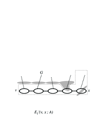
Figure 1: Schematic depiction of the events $E_{1}^{\prime}$ and $E_{2}^{\prime}$. Shaded regions represent the set $A$ and dotted lines represent possible but not mandatory connections in $C(v)$. The dashed lines indicate that the inner regions are $G$-free.

Next we observe that for $j=1,2$,

$$\langle I[E_{j}(v,x;A)]\rangle=\langle I[E_{j}^{\prime}(v,x;A)]\rangle+\sum_{(u^{\prime},v^{\prime})}\langle I[E_{j}(v,u^{\prime},v^{\prime},x;A)]\rangle.$$ (4.31)

We now claim that Lemma 4.3 can be applied to conclude that for $j=1,2$,

$$\langle I[E_{j}(v,u^{\prime},v^{\prime},x;A)]\rangle=p\langle I[E_{j}^{\prime\prime}(v,u^{\prime},v^{\prime};A)]\tau^{\tilde{C}^{\{u^{\prime},v^{\prime}\}}(v)}_{\vec{z},p}(v^{\prime},x)\rangle.$$ (4.32)

This can be seen as follows. By definition, $E_{j}(v,u^{\prime},v^{\prime},x;A)$ is the event that $E_{j}^{\prime}(v,u^{\prime};A)$ occurs, that $(u^{\prime},v^{\prime})$ is occupied and pivotal for $v\longleftrightarrow x$, and that $\tilde{C}^{\{u^{\prime},v^{\prime}\}}(x)\cap G=\emptyset$. It can be written as the intersection of the events that $E^{\prime}_{j}(v,u^{\prime};A)\mbox{ occurs on }\tilde{C}^{\{u^{\prime},v^{\prime}\}}(v)$, that $\{u^{\prime},v^{\prime}\}$ is occupied, and that $(v^{\prime}\longleftrightarrow x\;\&\;v^{\prime}\longleftrightarrow{/}\hskip 7.74998ptG)\mbox{ occurs in }{{{\mathbb{Z}}}^{d}}\backslash\tilde{C}^{\{u^{\prime},v^{\prime}\}}(v)$. Applying Lemma 4.3, we get

$$\langle I[E_{j}(v,u^{\prime},v^{\prime},x;A)]\rangle=p\langle I[E_{j}^{\prime\prime}(v,u^{\prime},v^{\prime};A)]\tau^{\tilde{C}^{\{u^{\prime},v^{\prime}\}}(v)}_{\vec{z},p}(v^{\prime},x)\rangle,$$ (4.33)

as required.

We are now in a position to generate an expansion. First, we introduce some abbreviated notation. Let $\tilde{C}_{n}=\tilde{C}_{n}^{\{u_{n},v_{n}\}}(v_{n-1})$, with $v_{-1}=0$, and let

$$X_{n} = I[E_{1}(v_{n-1},x;\tilde{C}_{n-1})]-I[E_{2}(v_{n-1},x;\tilde{C}_{n-1})],$$ (4.34)

$$X_{n}^{\prime} = I[E_{1}^{\prime}(v_{n-1},x;\tilde{C}_{n-1})]-I[E_{2}^{\prime}(v_{n-1},x;\tilde{C}_{n-1})],$$ (4.35)

$$X_{n}^{\prime\prime} = I[E_{1}^{\prime\prime}(v_{n-1},u_{n},v_{n};\tilde{C}_{n-1})]-I[E_{2}^{\prime\prime}(v_{n-1},u_{n},v_{n};\tilde{C}_{n-1})].$$ (4.36)

In terms of this new notation, (4.24) can be written as

$$\tau_{\vec{z},p}(0,x)=\langle I[E_{0}^{\prime}(0,x)]\rangle_{0}+p\sum_{(u_{0},v_{0})}\langle I[E_{0}^{\prime\prime}(0,u_{0},v_{0})]\rangle_{0}\tau_{\vec{z},p}(v_{0},x)-p\sum_{(u_{0},v_{0})}\langle I[E_{0}^{\prime\prime}(0,u_{0},v_{0})]\langle X_{1}\rangle_{1}\rangle_{0}.$$ (4.37)

In view of (4.31) and (4.32),

$$\langle X_{n}\rangle_{n}=\langle X^{\prime}_{n}\rangle_{n}+p\sum_{(u_{n},v_{n})}\langle X^{\prime\prime}_{n}\tau_{\vec{z},p}^{\tilde{C}_{n}}(v_{n},x)\rangle_{n}.$$ (4.38)

By (4.13) and (4.23),

$$\tau_{\vec{z},p}^{\tilde{C}_{n}}(v_{n},x)=\tau_{\vec{z},p}(v_{n},x)-\langle X_{n+1}\rangle_{n+1}.$$ (4.39)

With (4.38), this gives

$$\langle X_{n}\rangle_{n}=\langle X^{\prime}_{n}\rangle_{n}+p\sum_{(u_{n},v_{n})}\langle X^{\prime\prime}_{n}\rangle_{n}\tau_{\vec{z},p}(v_{n},x)-p\sum_{(u_{n},v_{n})}\langle X^{\prime\prime}_{n}\langle X_{n+1}\rangle_{n+1}\rangle_{n}.$$ (4.40)

An expansion can now be generated by recursively substituting (4.40) into (4.37). To further abbreviate the notation, in generating the expansion we omit all arguments related to sites and omit the products of $p$ with summations over $(u_{n},v_{n})$ that are associated with each product. The first few iterations then yield

$$\tau = \langle I[E_{0}^{\prime}]\rangle_{0}+\langle I[E_{0}^{\prime\prime}]\rangle_{0}\tau-\langle I[E_{0}^{\prime\prime}]\langle X_{1}\rangle_{1}\rangle_{0}$$ (4.41)

$$= \Big{(}\langle I[E_{0}^{\prime}]\rangle_{0}-\langle I[E_{0}^{\prime\prime}]\langle X_{1}^{\prime}\rangle_{1}\rangle_{0}\Big{)}+\Big{(}\langle I[E_{0}^{\prime\prime}]\rangle_{0}-\langle I[E_{0}^{\prime\prime}]\langle X^{\prime\prime}_{1}\rangle_{1}\rangle_{0}\Big{)}\tau+\langle I[E_{0}^{\prime\prime}]\langle X^{\prime\prime}_{1}\langle X_{2}\rangle_{2}\rangle_{1}\rangle_{0}$$

$$= \Big{(}\langle I[E_{0}^{\prime}]\rangle_{0}-\langle I[E_{0}^{\prime\prime}]\langle X_{1}^{\prime}\rangle_{1}\rangle_{0}+\langle I[E_{0}^{\prime\prime}]\langle X^{\prime\prime}_{1}\langle X_{2}^{\prime}\rangle_{2}\rangle_{1}\rangle_{0}\Big{)}$$

$$+\Big{(}\langle I[E_{0}^{\prime\prime}]\rangle_{0}-\langle I[E_{0}^{\prime\prime}]\langle X^{\prime\prime}_{1}\rangle_{1}\rangle_{0}+\langle I[E_{0}^{\prime\prime}]\langle X^{\prime\prime}_{1}\langle X_{2}^{\prime\prime}\rangle_{2}\rangle_{1}\rangle_{0}\Big{)}\tau$$

$$-\langle I[E_{0}^{\prime\prime}]\langle X^{\prime\prime}_{1}\langle X_{2}^{\prime\prime}\langle X_{3}\rangle_{3}\rangle_{2}\rangle_{1}\rangle_{0},$$

and so on.

To simplify expressions involving nested expectations, we will sometimes use ${\mathbb{E}}$ rather than $\langle\cdot\rangle$ to denote expectations. To organize the terms in the expansion, we introduce the following notation, for $n\geq 1$:

$$g_{\vec{z},p}^{(0)}(0,x) = \langle I[E_{0}^{\prime}(0,x)]\rangle={\mathbb{E}}I[E_{0}^{\prime}(0,x)],$$ (4.42)

$$g_{\vec{z},p}^{(n)}(0,x) = (-1)^{n}{\mathbb{E}}_{0}I[E_{0}^{\prime\prime}]{\mathbb{E}}_{1}X_{1}^{\prime\prime}\cdots{\mathbb{E}}_{n-1}X_{n-1}^{\prime\prime}{\mathbb{E}}_{n}X_{n}^{\prime},$$ (4.43)

$$\Pi_{\vec{z},p}^{(0)}(0,v_{0}) = p\sum_{u_{0}}\langle I[E_{0}^{\prime\prime}(0,u_{0},v_{0})]\rangle=p\sum_{u_{0}}{\mathbb{E}}I[E_{0}^{\prime\prime}(0,u_{0},v_{0})],$$ (4.44)

$$\Pi_{\vec{z},p}^{(n)}(0,v_{n}) = (-1)^{n}p\sum_{u_{n}}{\mathbb{E}}_{0}I[E_{0}^{\prime\prime}]{\mathbb{E}}_{1}X_{1}^{\prime\prime}\cdots{\mathbb{E}}_{n-1}X_{n-1}^{\prime\prime}{\mathbb{E}}_{n}X_{n}^{\prime\prime},$$ (4.45)

$$U_{\vec{z},p}^{(n)}(0,x) = (-1)^{n}{\mathbb{E}}_{0}I[E_{0}^{\prime\prime}]{\mathbb{E}}_{1}X_{1}^{\prime\prime}\cdots{\mathbb{E}}_{n-1}X_{n-1}^{\prime\prime}{\mathbb{E}}_{n}X_{n}.$$ (4.46)

In the above, the notation continues to omit sums over $(u_{j},v_{j})$ and factors of $p$ associated with each product. The terms $g^{(n)}$ account for the terms in (4.41) whose innermost expectation involves an $X$ bearing a single prime, the terms $\Pi^{(n)}$ account for the terms in (4.41) whose innermost expectation involves an $X$ bearing a double prime, and $U^{(n)}$ accounts for the single term whose innermost expectation involves an unprimed $X$. For each $N\geq 0$, the expansion can then be written as

$$\tau_{\vec{z},p}(0,x)=\sum_{n=0}^{N}g_{\vec{z},p}^{(n)}(0,x)+\sum_{n=0}^{N}\sum_{v_{n}}\Pi_{\vec{z},p}^{(n)}(0,v_{n})\tau_{\vec{z},p}(v_{n},x)+U_{\vec{z},p}^{(N+1)}(0,x).$$ (4.47)

For $z_{u}\equiv z=1$ the set $G$ of green sites is empty, and the event $E_{2}$, which requires connection to $G$, cannot occur. Therefore all terms involving $E_{2}$ events vanish for $z=1$. In this special case, (4.47) becomes the expansion of [25] and agrees also with the expansion of I.

Taking the Fourier transform of (4.47) and solving for $\hat{\tau}_{\vec{z},p}(k)$ gives, for each $N\geq 0$,

$$\hat{\tau}_{\vec{z},p}(k)=\frac{\sum_{n=0}^{N}\hat{g}_{\vec{z},p}^{(n)}(k)+\hat{U}_{\vec{z},p}^{(N+1)}(k)}{1-\sum_{n=0}^{N}\hat{\Pi}_{\vec{z},p}^{(n)}(k)}.$$ (4.48)

Existence of all Fourier transforms appearing in the right side of (4.48) will be shown in Section 5.1, for $p=p_{c}$, $z_{u}\in[0,a]$ with $a<1$, and for $d$ sufficiently large. The bounds of Section 5.1 will also provide the convergence of summations mentioned below (4.24) and tacitly assumed in the subsequent analysis. The bounds apply also to the simpler subcritical case of $p<p_{c}$, $z_{u}\in[0,1]$, but we omit any explicit discussion of this case.

5 Proof of Lemmas 2.1 and 2.2

Throughout this section, we restrict attention to $p=p_{c}$, and drop subscripts $p_{c}$ from the notation. We will define $g_{\vec{z}}(0,x)$ and $\Pi_{\vec{z}}(0,x)$ obeying (3.8) for $z_{u}\in[0,a]$, for any $a\in[0,1)$. This also gives (2.1) for $z\in[0,1)$. For constant $z_{u}=z$, $\hat{g}_{z}(k)$ and $\hat{\Pi}_{z}(k)$ will be shown to obey (2.2), and to extend to complex $z$ with $|z|\leq 1$. This involves taking the limit $N\rightarrow\infty$ in (4.48), with the term $\hat{U}_{\vec{z}}^{(N+1)}(k)$ vanishing in the limit. This will then give (2.1) and (2.2) for $|z|<1$. We will prove Lemmas 2.1 and 2.2 in Sections 5.1 and 5.2 respectively.

5.1 Proof of Lemma 2.1

We begin by stating two lemmas providing the estimates needed to obtain the identities (2.1), (2.2) and (3.8), and to prove Lemma 2.1. After stating the lemmas, we will show that these identities hold and prove Lemma 2.1, assuming the two lemmas. Then the two lemmas will be proved. Throughout this section, we assume without further mention that the dimension $d$ is sufficiently large. We remark that the use of $m_{2}=4$ in (5.2) requires us to take at least $d\geq 8$, but since we are not attempting to obtain estimates valid for all $d>6$ (for spread-out models), we have not tried to do without $m_{2}=4$.

Lemma 5.1.

(i) For $z_{u}\in[0,1]$ and $n\geq 0$, $|\hat{g}_{\vec{z}}^{(n)}(k)|\leq\sum_{x}|g_{\vec{z}}^{(n)}(0,x)|\leq O(d^{-n})$ and $|\hat{\Pi}_{\vec{z}}^{(n)}(k)|\leq\sum_{x}|\Pi_{\vec{z}}^{(n)}(0,x)|\leq O(d^{-n})$.
(ii) For $n\geq 0$ and constant $z_{u}\equiv z$, $\hat{g}_{z}^{(n)}(k)$ and $\hat{\Pi}_{z}^{(n)}(k)$ can be extended to complex $z$ with $|z|\leq 1$. For $|z|\leq 1$, $n\geq 0$, and $m_{1}=0,2$, $m_{2}=0,2,4$ their norms obey the bounds

$$\|\nabla_{k}^{m_{1}}\hat{g}_{z}^{(n)}(k)\| \leq \sum_{x}|x|^{m_{1}}\,\|g^{(n)}_{z}(0,x)\|\leq O(d^{-n}),$$ (5.1)

$$\|\nabla_{k}^{m_{2}}\hat{\Pi}_{z}^{(n)}(k)\| \leq \sum_{x}|x|^{m_{2}}\,\|\Pi^{(n)}_{z}(0,x)\|\leq O(d^{-n}).$$ (5.2)

Lemma 5.2.

Let $a\in[0,1)$. For $z_{u}\in[0,a]$, $k\in[-\pi,\pi]^{d}$, and $N\geq 0$, the remainder term $\hat{U}^{(N+1)}_{\vec{z}}(k)$ obeys the bound

$$|\hat{U}_{\vec{z}}^{(N+1)}(k)|\leq O(d^{-(N+1)})(1+\chi_{a}).$$ (5.3)

By Lemmas 5.1(i) and 5.2, (3.8) follows by taking the limit $N\rightarrow\infty$ in (4.48) and then taking the inverse Fourier transform. The functions ${\hat{g}}_{\vec{z}}(k)$ and $\mbox{${\hat{\Pi}}$}_{\vec{z}}(k)$ are given by

$${\hat{g}}_{\vec{z}}(k)=\sum_{n=0}^{\infty}{\hat{g}}_{\vec{z}}^{(n)}(k),\quad\mbox{${\hat{\Pi}}$}_{\vec{z}}(k)=\sum_{n=0}^{\infty}\mbox{${\hat{\Pi}}$}_{\vec{z}}^{(n)}(k).$$ (5.4)

Taking $z_{u}\equiv z\in[0,1)$ then gives

$${\hat{\tau}}_{z}(k)=\frac{{\hat{g}}_{z}(k)}{1-\mbox{${\hat{\Pi}}$}_{z}(k)}.$$ (5.5)

As power series in $z$, ${\hat{g}}_{z}(k)$ and $\mbox{${\hat{\Pi}}$}_{z}(k)$ converge absolutely for $|z|\leq 1$, by Lemma 5.1(ii). The left side of (5.5) is a power series that converges absolutely, and therefore defines an analytic function, for $z$ in $|z|<1$. The two series are therefore equal for $|z|<1$, and the right side extends the left side to $|z|\leq 1$. This proves (2.2), and by taking the inverse Fourier transform, also proves (2.1). Also, since (4.47) agrees with the expansion of I for $z=1$, the claim at the end of Section 2.1 that $\hat{g}_{1}(k)=\hat{\phi}_{h=0}(k)$ and $\hat{\Pi}_{1}(k)=\hat{\Phi}_{h=0}(k)$, where $\hat{\phi}_{h}(k)$ and $\hat{\Phi}_{h}(k)$ are the functions occuring in the one-$M$ scheme in (I.3.88), then follows.

Next, we prove Lemma 2.1, assuming Lemmas 5.1 and 5.2.

Proof of Lemma 2.1. The upper bounds of Lemma 2.1 are immediate consequences of Lemma 5.1, and we need only prove that ${\hat{g}}_{1}(0)$ and $-\nabla^{2}\mbox{${\hat{\Pi}}$}_{1}(0)$ are both equal to $1+O(d^{-1})$.

We begin with ${\hat{g}}_{1}(0)$. By (I.3.6), ${\hat{g}}^{(0)}_{1}(0)=\hat{\phi}^{(0)}_{h=0}(0)=1+\hat{\phi}_{h=0}^{(01)}(0)$, and we have

$${\hat{g}}_{1}(0)=1+\hat{\phi}_{h=0}^{(01)}(0)+\sum_{n=1}^{\infty}{\hat{g}}_{1}^{(n)}(0).$$ (5.6)

The bound (I.3.20) can easily be improved to $|\hat{\phi}_{h=0}^{(01)}(0)|\leq O(d^{-1})$. With Lemma 5.1(ii), this gives

$${\hat{g}}_{1}(0)=1+O(d^{-1})+\sum_{n=1}^{\infty}O(d^{-n})=1+O(d^{-1}).$$ (5.7)

Similarly, we have

$$\begin{split}-\nabla^{2}\mbox{${\hat{\Pi}}$}_{1}(0)&=\sum_{x}\sum_{n=0}^{\infty}|x|^{2}\Pi_{h=0}^{(n)}(0,x)\\ &=2dp_{c}+p_{c}\sum_{(u,v):u\neq 0}|v|^{2}\left\langle I[E_{0}^{\prime\prime}(0,u,v)]\right\rangle_{1}+\sum_{n=1}^{\infty}\sum_{x}|x|^{2}\Pi_{h=0}^{(n)}(0,x).\end{split}$$ (5.8)

The first term is $1+O(d^{-1})$ by (1.39). The second term can be bounded using the weighted bubble diagram ${\sf W}^{(2)}_{h=0,p_{c}}$ of (I.3.16), which was shown to be $O(d^{-1})$ in [25]. By Lemma 5.1, the third term is $O(d^{-1})$. This gives the desired result $-\nabla^{2}\mbox{${\hat{\Pi}}$}_{1}(0)=1+O(d^{-1})$. ∎

Proof of Lemma 5.1. The bounds obtained in part (ii) of the lemma are actually stronger than those needed for part (i), and we discuss only the proof of part (ii) here. Also, since $g$ and $\Pi$ are almost identical, we discuss only $g$.

To bound the norm in (5.1), we will use the fact that for a power series $f$ with real coefficients $a_{n}$ all of the same sign, the norm (2.3) obeys

$$\|f(z)\|=\sum_{n=0}^{\infty}|a_{n}||z|^{n}=|f(|z|)|.$$ (5.9)

We will explain in more detail below that, as power series in $z$, $g_{z}^{(n)}(0,x)$ and $\Pi_{z}^{(n)}(0,x)$ have real coefficients of varying signs. To handle a power series $f(z)$ with both positive and negative coefficients, our strategy will be to decompose it into a sum of functions $f_{j}(z)$ with coefficients of definite sign. Then we use the triangle inequality and (5.9) to conclude

$$\|f(z)\|\leq\sum_{j}\|f_{j}(z)\|=\sum_{j}|f_{j}(|z|)|,$$ (5.10)

and thus reduce the problem of estimating $\|f(z)\|$ to that of estimating $|f_{j}(|z|)|$.

Beginning with $g_{z}^{(0)}$, by definition

$$g_{z}^{(0)}(0,x)=\left\langle I[E_{0}^{\prime}(0,x)]\right\rangle=\left\langle I[E_{0,b}^{\prime}(0,x)]z^{|C(0)|}\right\rangle_{b},$$ (5.11)

where $E_{0,b}^{\prime}(0,x)$ is the bond event $\{0\Longleftrightarrow x\}$ and $\left\langle\cdot\right\rangle_{b}$ denotes expectation with respect to bond variables only. This can be written as a power series in $z$ with positive coefficients, and hence it extends to complex $z$ within the disk of convergence. Using (5.9), we argue as in (I.3.36) to obtain

$$\left\|g_{z}^{(0)}(0,x)\right\|=\left\langle I[E_{0,b}^{\prime}(0,x)]|z|^{|C(0)|}\right\rangle_{b}\leq\tau_{1}(0,x)^{2}.$$ (5.12)

Multiplying by $|x|^{m}$ and summing over $x$ then gives (5.1) for $n=0$, $|z|\leq 1$, using the methods of [25]. The case $m=4$ (which is needed for $\Pi_{z}$) did not occur in [25], but the methods there apply if we associate a factor $|x|^{2}$ to each factor $\tau_{1}(0,x)$ on the right side of (5.12).

For $n\geq 1$, we have

$$g_{z}^{(n)}(0,x)=(-1)^{n}{\mathbb{E}}_{0}I[E_{0}^{\prime\prime}]{\mathbb{E}}_{1}X_{1}^{\prime\prime}\cdots{\mathbb{E}}_{n-1}X_{n-1}^{\prime\prime}{\mathbb{E}}_{n}X_{n}^{\prime}.$$ (5.13)

We insert $X^{\prime\prime}=I[E_{1}^{\prime\prime}]-I[E_{2}^{\prime\prime}]$ in the above, and similarly for the inner expectation with $X^{\prime}$, and expand the products to obtain a sum of $\pm 1$ times expectations involving $E_{j}^{\prime}$ and $E_{j}^{\prime\prime}$. The bond connections required by the events $E_{j}^{\prime}$ and $E_{j}^{\prime\prime}$ are given in terms of the auxiliary bond events

$$E_{1,b}^{\prime}(v,x;A) \equiv \bigl{\{}v\stackrel{{\scriptstyle A}}{{\longleftrightarrow}}x\;\&\;\nexists\textrm{ pivotal }(u^{\prime},v^{\prime})\textrm{ for }v\longleftrightarrow x\textrm{ such that }v\stackrel{{\scriptstyle A}}{{\longleftrightarrow}}x\bigr{\}},$$ (5.14)

$$E_{1,b}^{\prime\prime}(v,u^{\prime},v^{\prime};A) \equiv E_{1,b}^{\prime}(v,u^{\prime};A)\mbox{ occurs on }\tilde{C}^{\{u^{\prime},v^{\prime}\}}(v),$$ (5.15)

$$E_{2,b}^{\prime}(v,x;A) \equiv \bigl{\{}v\longleftrightarrow x\mbox{ {\rm in} }{{{\mathbb{Z}}}^{d}}\backslash A\;\&\;\textrm{(last sausage of }v\longleftrightarrow x)\longleftrightarrow A\bigr{\}},$$ (5.16)

$$E_{2,b}^{\prime\prime}(v,u^{\prime},v^{\prime};A) \equiv E_{2,b}^{\prime}(v,u^{\prime};A)\mbox{ occurs on }\tilde{C}^{\{u^{\prime},v^{\prime}\}}(v).$$ (5.17)

The conditions due to the site variables, in $E_{j}^{\prime}$ and $E_{j}^{\prime\prime}$, can be expressed in terms of the subclusters $Y^{1}$, $Y^{2}$, $Y^{3}$ depicted in Figure 2 and defined as follows:

$$Y^{1} = (\mbox{last sausage of $v\longrightarrow x$})\cup\{y\in C(v):y\longleftrightarrow v\mbox{ in }{{{\mathbb{Z}}}^{d}}\backslash A\},$$ (5.18)

$$Y^{2} = \{y\in C(v):y\longleftrightarrow v\mbox{ in }{{{\mathbb{Z}}}^{d}}\backslash A\},$$ (5.19)

$$Y^{3} = (\mbox{last sausage of $v\longrightarrow x$})\backslash Y^{2}.$$ (5.20)

The above definitions are appropriate for $E_{1}^{\prime}$ and $E_{2}^{\prime}$. For $E_{1}^{\prime\prime}$ and $E_{2}^{\prime\prime}$, we define the $Y$’s to be the intersection of the above with $\tilde{C}^{\{u^{\prime},v^{\prime}\}}(v)$.

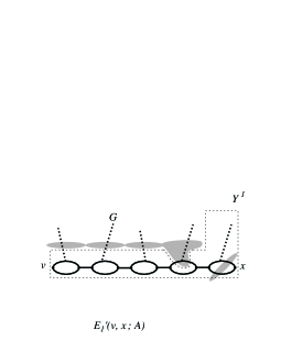
Figure 2: Schematic depiction of $Y^{1}$, $Y^{2}$, $Y^{3}$, and of the event $E_{3}^{\prime}$ defined under (6.14). Shaded regions represent the set $A$ and dotted lines represent possible but not mandatory connections in $C(v)$. For $E_{3}^{\prime}$, the dashed lines indicate that the inner region is $G$-free.

Using these definitions, and using $\langle\cdot\rangle_{s}$ and $\langle\cdot\rangle_{b}$ for expectations with respect to the site and bond variables, for $z\in[0,1]$ we have

$$\left\langle I[E_{1}^{\prime}(v,x;A)]\right\rangle_{s} = I[E_{1,b}^{\prime}(v,x;A)]\,z^{|Y^{1}|},$$ (5.21)

$$\left\langle I[E_{2}^{\prime}(v,x;A)]\right\rangle_{s} = I[E_{2,b}^{\prime}(v,x;A)]\,z^{|Y^{2}|}(1-z^{|Y^{3}|}),$$ (5.22)

$$\left\langle I[E_{1}^{\prime\prime}(v,u^{\prime},v^{\prime};A)]\right\rangle_{s} = I[E_{1,b}^{\prime\prime}(v,u^{\prime},v^{\prime};A)]\,z^{|Y^{1}|},$$ (5.23)

$$\left\langle I[E_{2}^{\prime\prime}(v,u^{\prime},v^{\prime};A)]\right\rangle_{s} = I[E_{2,b}^{\prime\prime}(v,u^{\prime},v^{\prime};A)]\,z^{|Y^{2}|}(1-z^{|Y^{3}|}).$$ (5.24)

Having expanded the $X$’s in (5.13), we insert (5.21)–(5.24), leaving only bond expectations. For terms involving $E_{2}$, we use

$$(1-z^{|Y^{3}|})z^{|Y^{2}|}=z^{|Y^{2}|}-z^{|Y^{2}|+|Y^{3}|},$$ (5.25)

and further expand to obtain a sum of terms in which the $z$-dependence of each term is simply a power determined by the $Y$’s. The result is a sum of terms, with coefficients $\pm 1$, of power series in $z$ having nonnegative coefficients. The number of terms resulting from these two expansions is at most $4^{n}$. This provides a formula which extends $g_{z}^{(n)}(0,x)$ to complex $z$ within any disk in which all the series converge. We will show that, in fact, when summed over $x$ the series all converge absolutely for $|z|\leq 1$.

Explicitly, we demonstrate the convergence for two examples only. The other cases are similar, using standard diagrammatic estimation. First, we consider the term involving only $E_{1}$-events. To bound

$$\left\|{\mathbb{E}}_{0,b}I[E_{0,b}^{\prime\prime}]z^{|\tilde{C}_{0}(0)|}{\mathbb{E}}_{1,b}I[E_{1,b}^{\prime\prime}]z^{|Y_{1}^{1}|}\cdots{\mathbb{E}}_{n-1,b}I[E_{1,b}^{\prime\prime}]z^{|Y_{n-1}^{1}|}{\mathbb{E}}_{n,b}I[E_{1,b}^{\prime}]z^{|Y_{n}^{1}|}\right\|,$$ (5.26)

we use (5.9) to effectively replace $z$ by $|z|$, and then bound $|z|$ by 1. We then bound the result using the BK inequality, exactly as was done for $\hat{\Phi}(k)$ in Section I.3.2, and obtain Feynman diagrams having propagator $\tau_{p_{c}}(0,x)$. If we sum over $x$, we get diagrams which can be bounded by triangles. With the presence of $|x|^{2}$, the situation is similar. For $|x|^{4}$, we can arrange that two different two-point functions each receive a factor $|x|^{2}$, and again standard methods apply.

For the diagrams involving at least one $E_{2}$ event, we proceed as outlined in the paragraph containing (5.25), and then bound all factors of $|z|$ by $1$. We are then left with bounding nested bond expectations. We illustrate the method for bounding these nested bond expectations by considering a specific contribution to the case $n=2$, given by

$$T(x)=p_{c}\sum_{(u_{0},v_{0})}p_{c}\sum_{(u_{1},v_{1})}\langle I[E_{0,b}^{\prime\prime}\langle I[E_{2,b}^{\prime\prime}]\langle I[E_{1,b}^{\prime}]\rangle_{2,b}\rangle_{1,b}\rangle_{0,b}.$$ (5.27)

The general case is similar, using the methods of [25]. The analysis is simplified by the fact that we are taking the dimension to be large, so that we can use squares and higher order diagrams in our bounds.

In this approach, the use of (5.25) loses any factors of $M_{z}$ that could be expected due to connections to $G$, and this prevents us from obtaining bounds for sufficiently spread-out models in all dimensions $d>6$. We do not know how to avoid the loss of the factors $M_{z}$ for complex $z$, though we were able to exploit these factors in I for real $z$. As was mentioned previously, the case $m_{2}=4$ in (5.2) also prevents us from handling all $d>6$. In addition, we will be encountering complicated diagrams in Sections 7 and 8, which also will prevent us from handling dimensions above but near $6$.

Using the BK inequality, we bound the innermost expectation $\langle I[E_{1,b}^{\prime}(v_{1},x;\tilde{C}_{1}^{\{u_{1},v_{1}\}}(v_{0}))]\rangle_{2}$ of (5.27) by

$$\begin{split}&\left\langle I[\exists w_{1}\in\tilde{C}_{1}^{\{u_{1},v_{1}\}}(v_{0}),\exists a\in{{{\mathbb{Z}}}^{d}},(v_{1}\longleftrightarrow a)\circ(a\longleftrightarrow w_{1})\circ(w_{1}\longleftrightarrow x)\circ(a\longleftrightarrow x)]\right\rangle_{2}\\ &\hskip 28.45274pt\leq\sum_{a,w_{1}\in{{{\mathbb{Z}}}^{d}}}I[w_{1}\in\tilde{C}_{1}^{\{u_{1},v_{1}\}}(v_{0})]\tau_{1}(v_{1},a)\tau_{1}(a,w_{1})\tau_{1}(w_{1},x)\tau(a,x).\end{split}$$ (5.28)

By (5.17), we can bound $\langle I[E_{2,b}^{\prime\prime}(v_{0},u_{1},v_{1};\tilde{C}_{0}^{\{u_{0},v_{0}\}}(0))]I[w_{1}\in\tilde{C}_{1}(v_{0})]\rangle_{1}$ above by

$$\begin{split}&\left\langle I[\exists w_{0}\in\tilde{C}_{0}^{\{u_{0},v_{0}\}}(0),(v_{0}\longleftrightarrow u_{1})\circ(u_{1}\longleftrightarrow w_{0})]I[w_{1}\longleftrightarrow v_{0}]\right\rangle\\ &\hskip 28.45274pt\leq\sum_{w_{0},t_{1}\in{{{\mathbb{Z}}}^{d}}}I[w_{0}\in\tilde{C}_{0}^{\{u_{0},v_{0}\}}(0)]\Big{(}\tau_{1}(v_{0},u_{1})\tau_{1}(u_{1},t_{1})\tau_{1}(t_{1},w_{0})\tau_{1}(t_{1},w_{1})\\ &\hskip 71.13188pt+\tau_{1}(v_{0},t_{1})\tau_{1}(t_{1},w_{1})\tau_{1}(t_{1},u_{1})\tau_{1}(u_{1},w_{0})\Big{)}.\end{split}$$ (5.29)

Finally, we bound $\langle I[E_{0,b}^{\prime\prime}(0,u_{0},v_{0})]I[w_{0}\in\tilde{C}_{0}^{\{u_{0},v_{0}\}}(0)]\rangle_{0}$ above by

$$\left\langle I[(0\longleftrightarrow u_{0})\circ(u_{0}\longleftrightarrow 0)]I[w_{0}\longleftrightarrow 0]\right\rangle\leq\sum_{t_{0}\in{{{\mathbb{Z}}}^{d}}}\tau_{1}(0,u_{0})\tau_{1}(u_{0},t_{0})\tau_{1}(t_{0},0)\tau_{1}(t_{0},w_{0})$$ (5.30)

Combining (LABEL:eq:T2inmost.1)–(5.30), we obtain as an upper bound for $T_{2}(x)$ the diagrams

Summed over $x$, these diagrams can be bounded using the triangle diagram. It is then routine to argue that, for $m=0,2,4$,

$$\sum_{x}|x|^{m}\|T_{2}(x)\|\leq O(d^{-2}).$$ (5.31)

For the case $m=4$, we require that $d\geq 10$.

General $n$ can be handled similarly. For example, a typical contribution arising in bounding ${\mathbb{E}}_{0,b}I[E_{0,b}^{\prime\prime}]{\mathbb{E}}_{1,b}I[E_{2,b}^{\prime\prime}]{\mathbb{E}}_{2,b}I[E_{2,b}^{\prime\prime}]{\mathbb{E}}_{3,b}I[E_{1,b}^{\prime\prime}]{\mathbb{E}}_{4,b}I[E_{2,b}^{\prime\prime}]$ is the diagram

Such diagrams can be bounded using the square diagram. The result, for $m=2,3,4$, is the bound

$$\sum_{x}|x|^{m}\|g_{z}^{(n)}(0,x)\|\leq O(d^{-n}).$$ (5.32)

The case $m=4$ is not needed for (5.1), but it is used in (5.2). Any value of $m$ can be handled, at the cost of increasing $d$. For $m=4$, we require $d\geq 12$. ∎

For the proof of Lemma 5.2, we will need the cut-the-tail Lemma I.3.5, which is restated as Lemma 5.3 below. Although stated in I for constant $z$, the proof of the cut-the-tail lemma extends immediately to site-dependent $z_{u}$. In its statement, $M_{\vec{z}}=P_{p_{c}}(0\longleftrightarrow G)$.

Lemma 5.3.

Let $x$ be a site, $\{u,v\}$ a bond, and $E$ an increasing event. Then for a set of sites $A$ with $A\ni u$, and for $p\leq p_{c}$ (assuming no infinite cluster at $p_{c}$) and $z_{y}\in[0,1]$ for all $y\in{{{\mathbb{Z}}}^{d}}$,

$$\left\langle{\rm I}[E\mbox{ occurs on }\tilde{C}^{\{u,v\}}(A)]\,\tau_{\vec{z}}^{\tilde{C}^{\{u,v\}}(A)}(v,x)\right\rangle\leq\frac{1}{1-pM_{\vec{z}}}\,{P(E)}\,\tau_{\vec{z}}(v,x).$$ (5.33)

Proof of Lemma 5.2. Beginning with the definition of the remainder term in (4.46), and expanding the factors of $X$ using (4.34)–(4.36) as in the proof of Lemma 5.1, $U^{(n)}_{\vec{z}}(0,x)$ can be estimated by

$$|U_{\vec{z}}^{(n)}(0,x)|\leq\sum_{\sigma_{j}=1,2}\left|\langle I_{0}^{\prime\prime}\langle I_{1,\sigma_{1}}^{\prime\prime}\langle\cdots\langle I_{n-1,\sigma_{n-1}}^{\prime\prime}\langle I_{n,\sigma_{n}}\rangle_{n}\rangle_{n-1}\cdots\rangle_{2}\rangle_{1}\rangle_{0}\right|$$ (5.34)

where $I_{\ell,\sigma}^{\prime\prime}$ represents $I[E_{\sigma}^{\prime\prime}]$ on the level-$\ell$ expectation, and $I_{n,\sigma}$ represents $I[E_{\sigma}]$ in the level-$n$ expectation. Combining (4.31) and (4.32), we have

$$\left\langle I[E_{j}(v,x;A)]\right\rangle=\left\langle I[E_{j}^{\prime}(v,x;A)]\right\rangle+p\sum_{(u^{\prime},v^{\prime})}\left\langle I[E_{j}^{\prime\prime}(v,u^{\prime},v^{\prime};A)]\tau_{\vec{z}}^{\tilde{C}^{\{u^{\prime},v^{\prime}\}}(v)}(v^{\prime},x)\right\rangle.$$ (5.35)

This identity is used for the innermost expectation $\langle I_{n,\sigma_{n}}\rangle$.

The first term of (5.35) is bounded as before, using the analogue of (5.21) and (5.22) for site-dependent variables. The result is

$$\left|\left\langle I[E_{1}^{\prime}(v,x;A)]\right\rangle\right| =\left|\left\langle I[E_{1,b}^{\prime}(v,x;A)]\,{\textstyle{\prod_{u\in Y^{1}}}}z_{u}\right\rangle_{b}\right|\leq\left\langle I[E_{1,b}^{\prime}(v,x;A)]\right\rangle_{b},$$ (5.36)

$$\left|\left\langle I[E_{2}^{\prime}(v,x;A)]\right\rangle\right| =\left|\left\langle I[E_{1,b}^{\prime}(v,x;A)]\,({\textstyle{\prod_{u\in Y^{2}}}}z_{u})(1-{\textstyle{\prod_{y\in Y^{3}}}}z_{y})\right\rangle_{b}\right|\leq 2\left\langle I[E_{1,b}^{\prime}(v,x;A)]\right\rangle_{b},$$ (5.37)

where in the second line we used $|(\prod_{u}z_{u})(1-\prod_{v}z_{v})|\leq 2$. The remaining diagrammatic estimation is routine, and yields a bound $O(d^{-n})$.

For the second term of (5.35), we use the cut-the-tail Lemma 5.3. In preparation, we note by analogy with (5.23) and (5.24) that

$$\left\langle I[E_{1}^{\prime\prime}(v,u^{\prime},v^{\prime};A)]\,\tau_{\vec{z}}^{\tilde{C}^{\{u^{\prime},v^{\prime}\}}(v)}(v^{\prime},x)\right\rangle \leq \left\langle I[E_{1,b}^{\prime\prime}(v,u^{\prime},v^{\prime};A)]\,\tau_{\vec{z}}^{\tilde{C}^{\{u^{\prime},v^{\prime}\}}(v)}(v^{\prime},x)\right\rangle_{b},$$ (5.38)

$$\left\langle I[E_{2}^{\prime\prime}(v,u^{\prime},v^{\prime};A)]\,\tau_{\vec{z}}^{\tilde{C}^{\{u^{\prime},v^{\prime}\}}(v)}(v^{\prime},x)\right\rangle \leq 2\left\langle I[E_{2,b}^{\prime\prime}(v,u^{\prime},v^{\prime};A)]\,\tau_{\vec{z}}^{\tilde{C}^{\{u^{\prime},v^{\prime}\}}(v)}(v^{\prime},x)\right\rangle_{b}.$$ (5.39)

To obtain increasing events for application of the cut-the-tail lemma, we note that

$$\bigl{\{}E_{1,b}^{\prime}(v,u^{\prime},v^{\prime};A)\mbox{ occurs on }\tilde{C}^{\{u^{\prime},v^{\prime}\}}\bigr{\}}\subset\bigcup_{a,b\in{{{\mathbb{Z}}}^{d}}}\bigl{\{}\bar{F}_{1}(v,u^{\prime},a,b;A)\mbox{ occurs on }\tilde{C}^{\{u^{\prime},v^{\prime}\}}\bigr{\}},$$ (5.40)

$$\bigl{\{}E_{2,b}^{\prime}(v,u^{\prime},v^{\prime};A)\mbox{ occurs on }\tilde{C}^{\{u^{\prime},v^{\prime}\}}\bigr{\}}\subset\bigcup_{a\in{{{\mathbb{Z}}}^{d}}}\bigl{\{}\bar{F}_{2}(v,u^{\prime},a;A)\mbox{ occurs on }\tilde{C}^{\{u^{\prime},v^{\prime}\}}\bigr{\}},$$ (5.41)

where

$$\bar{F}_{1}(v,u^{\prime},a,b;A) = \bigl{\{}(v\longleftrightarrow b)\circ(b\longleftrightarrow a)\circ(a\longleftrightarrow u^{\prime})\circ(b\longleftrightarrow u^{\prime})\bigr{\}}\cap\{a\in A\},$$ (5.42)

$$\bar{F}_{2}(v,u^{\prime},a;A) = \{(v\longleftrightarrow u^{\prime})\circ(u^{\prime}\longleftrightarrow a)\}\cap\{a\in A\}.$$ (5.43)

Now in this form, we can use Lemma 5.3. After applying Lemma 5.3, we use $\tau_{\vec{z}}(v^{\prime},x)\leq\tau_{a}(v^{\prime},x)$. The remaining diagrammatic estimation is routine. Summation of the factor $\tau_{a}(v^{\prime},x)$ over $x$ gives the factor $\chi_{a}$ in the statement of the lemma. ∎

5.2 Proof of Lemma 2.2

In this section, we prove Lemma 2.2, which asserts that $\hat{F}_{z}(k)$ obeys the bound $|\hat{F}_{z}(k)|\geq-Kd^{-1}+\frac{1}{2e}{\rm Re}[1-z\hat{D}(k)]$ for high $d$, when $p=p_{c}$, uniformly in $|z|<1$, and $k\in[-\pi,\pi]^{d}$.

By (2.9), $\hat{\Pi}_{1}(0)=1$, and hence $\hat{F}_{z}(k)=\mbox{${\hat{\Pi}}$}_{1}(0)-\mbox{${\hat{\Pi}}$}_{z}(k)$. We write this as $\hat{F}_{z}(k)=A_{1}+A_{2}$, with $A_{1}$ and $A_{2}$ defined by

$$A_{1} = p_{c}\sum_{(0,v)}\left[\left\langle I[E^{\prime\prime}_{0}(0,0,v)]\right\rangle_{1}-\left\langle I[E^{\prime\prime}_{0}(0,0,v)]\right\rangle_{z}e^{ik\cdot v}\right],$$ (5.44)

$$A_{2} = p_{c}\sum_{(u,v):u\neq 0}\left[\left\langle I[E^{\prime\prime}_{0}(0,u,v)]\right\rangle_{1}-\left\langle I[E^{\prime\prime}_{0}(0,u,v)]\right\rangle_{z}e^{ik\cdot v}\right]+\sum_{n=1}^{\infty}\left[\mbox{${\hat{\Pi}}$}_{1}^{(n)}(0)-\mbox{${\hat{\Pi}}$}_{z}^{(n)}(k)\right].$$ (5.45)

The first term on the right side of (5.45) is $O(d^{-1})$ by Lemma I.3.4 and (1.39), as follows. In the notation of Lemma I.3.4, this term is $\hat{\Phi}^{(01)}_{0}(k)-\hat{\Phi}^{(01)}_{h}(k)$, which is bounded above in absolute value by $|\hat{\Phi}^{(01)}_{0}(k)|+|\hat{\Phi}^{(01)}_{h}(k)|$. The $z$-dependence of the second term is dominated by its value when $z=1$, and the bound of Lemma I.3.4is easily seen to be $O(d^{-1})$, so that $|\hat{\Phi}^{(01)}_{0}(k)|+|\hat{\Phi}^{(01)}_{h}(k)|\leq O(d^{-1})$. Therefore, by Lemma 5.1,

$$|A_{2}|\leq O(d^{-1})+\sum_{n=1}^{\infty}O(d^{-n})=O(d^{-1}).$$ (5.46)

The main term $A_{1}$ is, by definition, given by

$$A_{1}=p_{c}\sum_{(0,v)}\sum_{n=1}^{\infty}\left\langle I[|\tilde{C}^{\{0,v\}}(0)|=n]\right\rangle_{b}\left(1-z^{n}e^{ik\cdot v}\right).$$ (5.47)

First we bound $|A_{1}|$ below by ${\rm Re}A_{1}$. Since ${\rm Re}(1-z^{n}e^{ik\cdot v})\geq 0$, we obtain a further lower bound by discarding the terms $n\geq 2$. The result is

$$|A_{1}|\geq{\rm Re}A_{1}\geq p_{c}\sum_{(0,v)}{P(|\tilde{C}^{\{0,v\}}(0)|=1)}{\rm Re}\left[1-ze^{ik\cdot v}\right]=2dp_{c}(1-p_{c})^{2d-1}{\rm Re}\left[1-z{\hat{D}}(k)\right].$$ (5.48)

By (1.39), $2dp_{c}(1-p_{c})^{2d-1}\geq\frac{1}{2e}$. Combined with (5.48) and (5.46), this proves Lemma 2.2. ∎

6 The $z$-derivative of $\Pi_{z}$: the second expansion

The quantities $\Gamma_{z}$ and $\Psi_{z}$ were defined in (2.6)–(2.7) to obey, for $z\in[0,1)$,

$$z\frac{d}{dz}g_{z}(0,x)=\chi_{z}\Gamma_{z}(0,x),\quad\quad z\frac{d}{dz}\Pi_{z}(0,x)=\chi_{z}\Psi_{z}(0,x).$$ (6.1)

In addition, (3.11)–(3.12) require that we identify functions $\Gamma_{z}^{(3)}$ and $\Psi_{z}^{(3)}$ which obey

$$z_{y}\frac{\partial}{\partial z_{y}}g_{\vec{z}}(0,x)=\sum_{v}\Gamma^{(3)}_{\vec{z}}(0,x,v)\tau_{\vec{z}}(v,y),\quad\quad z_{y}\frac{\partial}{\partial z_{y}}\Pi_{\vec{z}}(0,x)=\sum_{v}\Psi^{(3)}_{\vec{z}}(0,x,v)\tau_{\vec{z}}(v,y).$$ (6.2)

Because $g_{\vec{z}}$ and $\Pi_{\vec{z}}$ are almost identical, we consider only $\Pi_{\vec{z}}$ and $\Psi_{\vec{z}}$ explicitly. A similar analysis will apply for $g_{\vec{z}}$ and $\Gamma_{\vec{z}}$.

In this section, we will derive an expression for $\Psi^{(3)}_{\vec{z}}(0,x,v)$. This will also provide an expression for $\Psi_{z}(0,x)$. In fact, using (6.1) and (6.2), it follows by summing over $y$ and setting $z_{y}\equiv z$ that

$$\sum_{y}z_{y}\left.\frac{\partial}{\partial z_{y}}\Pi_{\vec{z}}(0,x)\right|_{z_{y}=z}=z\frac{d}{dz}\Pi_{z}(0,x)=\chi_{z}\Psi_{z}(0,x)=\chi_{z}\sum_{a}\Psi^{(3)}_{\vec{z}}(0,x,a).$$ (6.3)

Therefore,

$$\Psi_{z}(0,x)=\sum_{a}\Psi^{(3)}_{\vec{z}}(0,x,a),\qquad\hat{\Psi}_{z}(k)=\hat{\Psi}^{(3)}_{z}(k,0).$$ (6.4)

In particular, this yields the claim in Lemma 3.1(i) that $\hat{\Psi}^{(3)}_{1}(0,0)=\hat{\Psi}_{1}(0)$.

The quantities $\Gamma$ and $\Psi$ will be defined by means of a second expansion, as in the differentiation of $\Phi_{z}$ in Section I.5. However, in the differentiation of $\Phi_{z}$ the second expansion was performed using the one-$M$ scheme, whereas here we will employ the more extensive expansion of Section 4. Throughout this section, we consider $z_{u}\in[0,a]$ with $a<1$, and we fix $p=p_{c}$.

6.1 The differentiation

In this section, we will derive an expression for the derivatives of $\Pi$ in (6.1) and (6.2). To differentiate $\Pi_{\vec{z}}(0,x)$, we recall from (4.45) that this is given as the sum over $N$ of

$$\Pi^{(N)}_{\vec{z}}(0,x)=(-1)^{N}p_{c}\sum_{u_{N}}{\mathbb{E}}_{0}I[E_{0}^{\prime\prime}]{\mathbb{E}}_{1}X_{1}^{\prime\prime}\cdots{\mathbb{E}}_{N-1}X_{N-1}^{\prime\prime}{\mathbb{E}}_{N}X_{N}^{\prime\prime}\quad(N=0,1,2,\ldots).$$ (6.5)

Here the nested expectations are performed from right to left, $X_{n}^{\prime\prime}=I[E_{1}^{\prime\prime}(v_{n-1},u_{n},v_{n};\tilde{C}_{n-1})]-I[E_{2}^{\prime\prime}(v_{n-1},u_{n},v_{n};\tilde{C}_{n-1})]$, summations $p_{c}\sum_{(u_{0},v_{0})}\cdots p_{c}\sum_{(u_{N-1},v_{N-1})}$ are tacitly understood on the right side, and we write ${\mathbb{E}}$ in place of $\langle\cdot\rangle$ to denote a joint bond/site expectation. Therefore, $\Pi^{(N)}_{\vec{z}}(0,x)$ is given by a sum of $2^{N}$ terms involving

$${\mathbb{E}}_{0}I[E_{0}^{\prime\prime}]{\mathbb{E}}_{1}I[E_{\sigma_{1}}^{\prime\prime}]\cdots{\mathbb{E}}_{N-1}I[E_{\sigma_{N-1}}^{\prime\prime}]{\mathbb{E}}_{N}I[E_{\sigma_{N}}^{\prime\prime}],$$ (6.6)

with each $\sigma_{n}$ equal to $1$ or $2$.

Before proceeding further, we recall an observation from Example I.4.5 that will be used repeatedly in what follows. By the definition of “occurs on $\tilde{C}$” in Definition 4.2(c), an expectation involving $E_{\sigma}^{\prime\prime}$ can be written as a conditional expectation of $E_{\sigma}^{\prime}(v_{n-1},u_{n};A)$, under the condition that $\{u_{n},v_{n}\}$ is vacant. We will write $\tilde{{\mathbb{E}}}$ or $\left\langle\,\cdot\,\right\rangle^{\tilde{}}$ for this conditional expectation. In the conditional expectations, we may replace $E_{\sigma}^{\prime\prime}$ events by $E_{\sigma}^{\prime}$, and we may drop the tilde from $\tilde{C}_{n}^{\{u_{n},v_{n}\}}(v_{n-1})$, since $C_{n}=C_{n}(v_{n-1})$ is then equal to $\tilde{C}_{n}^{\{u_{n},v_{n}\}}(v_{n-1})$. Therefore (6.6) can be rewritten as

$${\mathbb{E}}_{0}I[E_{0}^{\prime\prime}]\cdots{\mathbb{E}}_{n-1}I[E_{\sigma_{n-1}}^{\prime\prime}]\tilde{{\mathbb{E}}}_{n}I[E_{\sigma_{n}}^{\prime}]\tilde{{\mathbb{E}}}_{n+1}I[E_{\sigma_{n+1}}^{\prime}]{\mathbb{E}}_{n+2}I[E_{\sigma_{n+2}}^{\prime\prime}]\cdots{\mathbb{E}}_{N}I[E_{\sigma_{N}}^{\prime\prime}].$$ (6.7)

Our goal is to differentiate (6.7) with respect to $z_{y}$. Its $z_{y}$-dependence resides in the $z_{y}$-dependence of each of the nested expectations. For any individual expectation, the form of this dependence is different for $\sigma=1$ and $\sigma=2$, and can easily be given explicitly with the help of the clusters $Y^{1},Y^{2},Y^{3}$ depicted in Figure 2. By definition, $Y^{2}$ and $Y^{3}$ are disjoint. To simplify the notation, given a finite set $Y\subset{{{\mathbb{Z}}}^{d}}$, we will write

$$z^{Y}=\prod_{u\in Y}z_{u}.$$ (6.8)

The $z$-dependence of an expectation involving $E_{1}^{\prime}$ is $z^{Y^{1}}$, and that of an expectation involving $E_{2}^{\prime}$ is $z^{Y^{2}}(1-z^{Y^{3}})$. The overall $z$-dependence of the nested expectation is thus a product of such factors, and the differentiation can be performed using the product rule, with one term arising from differentiation of the $z$-dependence associated with each of the $N+1$ expectations. Each of the $2^{N}$ terms (6.7) thus gives rise, after application of $z_{y}\frac{\partial}{\partial z_{y}}$, to $N+1$ terms of the form

$${\mathbb{E}}_{0}I[E_{0}^{\prime\prime}]\cdots{\mathbb{E}}_{n-1}I[E_{\sigma_{n-1}}^{\prime\prime}]z_{y}\frac{\partial}{\partial z_{y}}\tilde{{\mathbb{E}}}_{n}I[E_{\sigma_{n}}^{\prime}]\tilde{{\mathbb{E}}}_{n+1}I[E_{\sigma_{n+1}}^{\prime}]{\mathbb{E}}_{n+2}I[E_{\sigma_{n+2}}^{\prime\prime}]\cdots{\mathbb{E}}_{N}I[E_{\sigma_{N}}^{\prime\prime}],$$ (6.9)

with only the $z$-dependence of the $n^{\rm th}$ expectation being differentiated. The case $n=0$ involves no new difficulties compared to the other values of $n$, and will not be discussed explicitly in what follows.

When $E_{\sigma_{n}}^{\prime}=E_{1}^{\prime}$, differentiation gives

$$z_{y}\frac{\partial}{\partial z_{y}}z^{Y^{1}}=I[y\in Y^{1}]\,z^{Y^{1}},$$ (6.10)

while for $E_{2}^{\prime}$, differentiation gives

$$z_{y}\frac{\partial}{\partial z_{y}}z^{Y^{2}}(1-z^{Y^{3}})=I[y\in Y^{2}]z^{Y^{2}}(1-z^{Y^{3}})-I[y\in Y^{3}]z^{Y^{2}}z^{Y^{3}}.$$ (6.11)

The factors $I[y\in Y]$ appearing in the above entail a connection to $y$ within the $n^{\rm th}$ expectation. We wish to “cut off” this connection at a suitable pivotal bond $(a^{\prime},a)$, to extract a factor $\tau_{\vec{z}}(a,x)$ from (6.9). However, to do so requires dealing with the fact that this connection to $y$ is not an independent event, and we handle this by means of a second application of the expansion. This second application of the expansion is in principle similar to the first application of the expansion in Section 4, but in practice it is more technical and complicated. The derivation of the second expansion will be completed in Section 6.3. The second expansion will then be bounded in Section 7. The analysis is similar to that of Section I.5.

After differentiation of the $n^{\rm th}$ expectation, three possibilities occur for this expectation. When $\sigma_{n}=1$, the $n^{\rm th}$ expectation contains

$$I[E_{1}^{\prime}]I[y\in Y^{1}].$$ (6.12)

When $\sigma_{n}=2$, two terms result. The first term on the right side of (6.11) produces

$$I[E_{2}^{\prime}]I[y\in Y^{2}].$$ (6.13)

The second term on the right side of (6.11) produces (with a minus sign)

$$I[E_{3}^{\prime}]I[y\in Y^{3}],$$ (6.14)

for a new event $E_{3}^{\prime}(v_{n-1},u_{n};C_{n-1})$ which is defined as follows. Let $S$ denote the last sausage for the connection from $v_{n-1}$ to $u_{n}$. Then

$E_{3}^{\prime}(v_{n-1},u_{n};C_{n-1})$ is the intersection of the events: (i) $v_{n-1}\longleftrightarrow u_{n}\in{{{\mathbb{Z}}}^{d}}\backslash C_{n-1}$, (ii) $S\cap G=\emptyset$, (iii) $S\cap C_{n-1}\neq\emptyset$ (i.e. $Y^{3}$ is not empty), and (iv) if $\exists g\in(C(v_{n-1})\backslash S)\cap G$, then $v_{n-1}\stackrel{{\scriptstyle C_{n-1}}}{{\longleftrightarrow}}g$.

The event $E_{3}^{\prime}$ was depicted in Figure 2. This unifies (6.12)–(6.14) and allows us to write (6.9) as a sum of terms of the form

$${\mathbb{E}}_{0}I[E_{0}^{\prime\prime}]\cdots{\mathbb{E}}_{n-1}I[E_{\sigma_{n-1}}^{\prime\prime}]\tilde{{\mathbb{E}}}_{n}I[E_{\nu}^{\prime}]I[y\in Y^{\nu}]\tilde{{\mathbb{E}}}_{n+1}I[E_{\sigma_{n-1}}^{\prime}]{\mathbb{E}}_{n+2}I[E_{\sigma_{n+2}}^{\prime\prime}]\cdots{\mathbb{E}}_{N}I[E_{\sigma_{N}}^{\prime\prime}]\quad(\nu=1,2,3).$$ (6.15)

6.2 The cutting lemma

Our task is to perform an expansion to cut off a factor of $\tau_{\vec{z}}(a,y)$ corresponding to the connection to $y\in Y^{\nu}$ in (6.15). This requires the identification of a “cutting bond,” where the connection to $y$ will be severed. We wish to cut off a $G$-free connection to $y$, which will be possible since by definition $Y^{\nu}\cap G=\emptyset$ for $\nu=1,2,3$.

We begin by narrowing the focus in (6.15) to the two relevant expectations

$$\cdots\tilde{{\mathbb{E}}}_{n}I[E_{\nu}^{\prime}]I[y\in Y^{\nu}]\tilde{{\mathbb{E}}}_{n+1}I[E_{\sigma_{n+1}}^{\prime}]\cdots\quad(\nu=1,2,3;\sigma_{n+1}=1,2).$$ (6.16)

Note that the event $\left\{y\in Y^{\nu}\right\}$ only makes sense when it occurs in conjunction with the event $E_{\nu}^{\prime}$. The $(n+1)^{\rm st}$ expectation is relevant, because $E_{\sigma_{n+1}}^{\prime}$ depends on the cluster $C_{n}$. We apply Fubini’s theorem to interchange the $n^{{\rm th}}$ and $(n+1)^{{\rm st}}$ bond/site expectations, to write (6.16) as

$$\cdots\tilde{{\mathbb{E}}}_{n+1}\tilde{{\mathbb{E}}}_{n}I[E_{\nu}^{\prime}]I[y\in Y^{\nu}]I[E_{\sigma_{n+1}}^{\prime}]\cdots.$$ (6.17)

We will work within the expectation $\tilde{{\mathbb{E}}}_{n}$, regarding the clusters of levels $0,\ldots,n-1$ and $n+1$ as being fixed.

The event $E_{\sigma_{n+1}}^{\prime}$ can be decomposed as an intersection of events on levels $n$ and $n+1$, as

$$E_{\sigma_{n+1}}^{\prime}(v_{n},u_{n+1};C_{n})_{n+1}=E_{\sigma_{n+1},0}(v_{n},u_{n+1})_{n+1}\cap J_{\rm cut}^{(\sigma_{n+1})}(C_{n+1})_{n},$$ (6.18)

where we have introduced an event $E_{\sigma_{n+1},0}$ which ensures that $C_{n+1}$ contains certain bond connections and an event $J_{\rm cut}^{(\sigma_{n+1})}(C_{n+1})_{n}$ which forces $C_{n}$ to be compatible with $C_{n+1}$. More precisely, the events $E_{\sigma_{n+1},0}$ are defined by

$$E_{1,0}(v_{n},u_{n+1})_{n+1}= \left\{v_{n}\longleftrightarrow u_{n+1}\;\&\;\tilde{C}^{\{u_{n+1}^{\prime},v_{n+1}^{\prime}\}}(u_{n+1})\cap G_{n+1}=\emptyset\right\},$$ (6.19)

$$E_{2,0}(v_{n},u_{n+1})_{n+1}= \left\{v_{n}\longleftrightarrow u_{n+1}\;\&\;\tilde{C}^{\{u_{n+1}^{\prime},v_{n+1}^{\prime}\}}(u_{n+1})\cap G_{n+1}\neq\emptyset\right\},$$

with $(u_{n+1}^{\prime},v_{n+1}^{\prime})$ the last pivotal bond for the level-$(n+1)$ connnection from $v_{n}$ to $u_{n+1}$. If there is no such pivotal bond, then $\tilde{C}^{\{u_{n+1}^{\prime},v_{n+1}^{\prime}\}}(u_{n+1})$ is to be interpreted as $C(u_{n+1})$. The events $J_{\rm cut}^{(\sigma_{n+1})}(C_{n+1})_{n}$ are defined by

$$J_{\rm cut}^{(1)}(C_{n+1})_{n}= \Bigl{\{}C_{n}\textrm{ intersects }C_{n+1}\textrm{ such that the level-$(n+1)$ connections satisfy:}$$

$$\left(v_{n+1}^{\prime}\Longleftrightarrow u_{n+1}\textrm{ through }C_{n}\right)\;\&\;\left(v_{n}\longleftrightarrow u_{n+1}^{\prime}\mbox{ {\rm in} }{{{\mathbb{Z}}}^{d}}\backslash C_{n}\right)$$

$$\;\&\;\left(\textrm{if }\exists g\in\tilde{C}^{\{u_{n+1}^{\prime},v_{n+1}^{\prime}\}}(v_{n})\cap G_{n+1}\textrm{ then }v_{n+1}^{\prime}\stackrel{{\scriptstyle C_{n}}}{{\longleftrightarrow}}g\right)\Bigr{\}},$$ (6.20)

$$J_{\rm cut}^{(2)}(C_{n+1})_{n}= \Bigl{\{}C_{n}\textrm{ intersects }C_{n+1}\textrm{ such that the level-$(n+1)$ connections satisfy:}$$

$$\left((u_{n+1}\stackrel{{\scriptstyle C_{n}}}{{\longleftrightarrow}}G_{n+1})\mbox{ {\rm in} }(\textrm{ last sausage of }v_{n}\longleftrightarrow u_{n+1})\right)\;\&\;\left(v_{n}\longleftrightarrow u_{n+1}\mbox{ {\rm in} }{{{\mathbb{Z}}}^{d}}\backslash C_{n}\right)$$

$$\;\&\;\left(\textrm{if }\exists g\in\tilde{C}^{\{u_{n+1}^{\prime},v_{n+1}^{\prime}\}}_{n+1}(v_{n})\cap G_{n+1}\textrm{ then }v_{n+1}^{\prime}\stackrel{{\scriptstyle C_{n}}}{{\longleftrightarrow}}g\right)\Bigr{\}}.$$ (6.21)

Thus we can rewrite (6.17) as

$$\cdots\tilde{{\mathbb{E}}}_{n+1}I[E_{\sigma_{n+1},0}(v_{n},u_{n+1})_{n+1}]\tilde{{\mathbb{E}}}_{n}I[E_{\nu}^{\prime}]_{n}I[y\in Y^{\nu}]_{n}I[J_{\rm cut}^{(\sigma_{n+1})}(C_{n+1})_{n}]\cdots.$$ (6.22)

Defining

$$J_{\nu,\sigma_{n+1}}(y)=E_{\nu}^{\prime}(v_{n-1},u_{n};C_{n-1})\cap\{y\in Y^{\nu}\}\cap J_{\rm cut}^{(\sigma_{n+1})}(C_{n+1}),$$ (6.23)

(6.22) can be rewritten as

$$\cdots\tilde{{\mathbb{E}}}_{n+1}I[E_{\sigma_{n+1},0}(v_{n},u_{n+1})_{n+1}]\tilde{{\mathbb{E}}}_{n}I[J_{\nu,\sigma_{n+1}}(y)_{n}]\cdots.$$ (6.24)

We now choose the “cutting bond” $(a^{\prime},a)$. We recall the existence of an ordering of the pivotal bonds for the connection from a site to a set of sites, as defined in Definition 4.1(d). The cutting bond is defined to be the last pivotal bond $(a^{\prime},a)$ for the connection $y\rightarrow\{v_{n-1},u_{n}\}\cup C_{n+1}\cup C_{n-1}$. It is possible that no such pivotal bond exists, and in that case, no expansion will be required.

Figure 3: Two examples of the choice of cutting bond $(a^{\prime},a)$. Solid lines represent $C_{n}$, dashed lines represent $C_{n-1}$, and bold dashed lines represent $C_{n+1}$.

In choosing the cutting bond, we require it to be pivotal for $\{v_{n-1},u_{n}\}$ to preserve (on the $a$ side of the cluster $C_{n}$) the backbone structure of the cluster $C_{n}$ which is required by $E_{\nu}^{\prime}(v_{n-1},u_{n};C_{n-1})$. We require the cutting bond to be pivotal for $C_{n+1}$ to ensure that we do not cut off as a tail something which may be needed to ensure that the last sausage of $C_{n+1}$ is connected through $C_{n}$, or that a previous sausage of $C_{n+1}$ is connected to $G_{n+1}$ through $C_{n}$. Finally, we require the cutting bond to be pivotal for the connection to $C_{n-1}$ because connections to $G$ must pass through $C_{n-1}$ and hence this realizes our goal to cut off a $G$-free connection to $y$. The above choice of the cutting bond is simpler than that of Section I.5.3. We do not expect our choice here to allow for dimensions near $d=6$ to be handled, but it will simplify our analysis.

Recall the definition of $\tilde{C}^{(a,a^{\prime})}(A)$ given in Definition 4.1. We now define several events, depending on $y,v_{n-1},u_{n},C_{n-1},C_{n+1}$, but to simplify the notation we make only the $y$-dependence explicit in the notation. We also make the abbreviation

$$A_{n}=\{v_{n-1},u_{n}\}\cup C_{n+1}\cup C_{n-1}.$$ (6.25)

Let

$$J_{\nu,\sigma_{n+1}}^{\prime}(y)_{n}=\, J_{\nu,\sigma_{n+1}}(y)_{n}\cap\left\{y\Longleftrightarrow A_{n}\right\},$$ (6.26)

$$J_{\nu,\sigma_{n+1}}^{\prime\prime}(a,a^{\prime})_{n}=\, \{J_{\nu,\sigma_{n+1}}^{\prime}(a)_{n}\mbox{ occurs on }\tilde{C}_{n}^{\{a,a^{\prime}\}}(A_{n})\},$$ (6.27)

$$J_{\nu,\sigma_{n+1}}(a,a^{\prime},y)_{n}=\, J_{\nu,\sigma_{n+1}}(y)_{n}\cap\left\{(a^{\prime},a)\textrm{ is the last occupied pivotal bond for }y\rightarrow A_{n}\right\}.$$ (6.28)

The overall level-$n$ event $J_{\nu,\sigma_{n+1}}(y)_{n}$ can be written as the disjoint union

$$J_{\nu,\sigma_{n+1}}(y)_{n}=J_{\nu,\sigma_{n+1}}^{\prime}(y)_{n}\bigcup^{\cdot}\biggl{(}\bigcup_{(a,a^{\prime})}^{\cdot}J_{\nu,\sigma_{n+1}}(a,a^{\prime},y)_{n}\biggr{)}.$$ (6.29)

In (6.29), configurations in $J_{\nu,\sigma_{n+1}}(y)_{n}$ have been classified according to the last pivotal bond $(a^{\prime},a)$. The appearance of $J_{\nu,\sigma_{n+1}}^{\prime}$ corresponds to the possibility that there is no such pivotal bond. For the configurations in which there is a pivotal bond, we will use the following important lemma.

Lemma 6.1.

For $\nu=1,2,3$ and $\sigma_{n+1}=1,2$,

$$J_{\nu,\sigma_{n+1}}(a,a^{\prime},y)_{n}=\, J_{\nu,\sigma_{n+1}}^{\prime\prime}(a,a^{\prime})_{n}\cap\left\{(y\longleftrightarrow a^{\prime}\;\&\;y\longleftrightarrow{/}\hskip 7.74998ptG)\mbox{ occurs in }{{{\mathbb{Z}}}^{d}}\backslash\tilde{C}_{n}^{\{a,a^{\prime}\}}(A_{n})\right\}$$

$$\cap\left\{\{a,a^{\prime}\}\textnormal{ is occupied}\right\}.$$ (6.30)

Before proving the lemma, we note that together with (6.29) and Lemma 4.3 it implies the identity

$$\left\langle I[J_{\nu,\sigma_{n+1}}(y)_{n}]\right\rangle_{n}^{\tilde{}}=\left\langle I[J_{\nu,\sigma_{n+1}}^{\prime}(y)_{n}]\right\rangle_{n}^{\tilde{}}+p\sum_{(a,a^{\prime})}\langle I[J_{\nu,\sigma_{n+1}}^{\prime\prime}(a,a^{\prime})_{n}]\,\tau_{z}^{\tilde{C}_{n}^{\{a,a^{\prime}\}}(A_{n})}(a^{\prime},y)\rangle_{n}^{\tilde{}}.$$ (6.31)

This will be the point of departure for the second expansion. We have actually employed a minor modification of Lemma 4.3 to the conditional expectation $\langle\cdot\rangle^{\tilde{}}$, and initially the restricted two-point function appearing in the above equation should be with respect to the conditional, rather than the usual expectation. However, there is no difference between the two. To see this, note that the event that $a^{\prime}\longleftrightarrow y$ in ${{{\mathbb{Z}}}^{d}}\backslash\tilde{C}_{n}^{\{a,a^{\prime}\}}(A_{n})$ is independent of the bond $\{u_{n},v_{n}\}$, since this bond touches the set $\tilde{C}_{n}^{\{a,a^{\prime}\}}(A_{n})$. Therefore either expectation can be used for the restricted two-point function, and for simplicity, we will use the ordinary unconditional expectation.

Proof of Lemma 6.1. To abbreviate the notation, we define

$$E_{\rm piv}=\{(a^{\prime},a)\textrm{ is pivotal for }y\rightarrow A_{n}\}.$$ (6.32)

We will show below that

$$\begin{split}J_{\nu,\sigma_{n+1}}(a,a^{\prime},y)_{n}=&\{J_{\nu,\sigma_{n+1}}(a)_{n}\mbox{ occurs on }\tilde{C}^{\{a,a^{\prime}\}}(A_{n})\}\\ &\cap\{(y\longleftrightarrow a^{\prime}\;\&\;y\longleftrightarrow{/}\hskip 7.74998ptG)\mbox{ occurs in }{{{\mathbb{Z}}}^{d}}\backslash\tilde{C}^{\{a,a^{\prime}\}}(A_{n})\}\\ &\cap\left\{\{a,a^{\prime}\}\textrm{ is occupied }\right\}\cap E_{\rm piv}.\end{split}$$ (6.33)

By Lemma 4.4, $E_{\rm piv}=\{a\longleftrightarrow A_{n}\mbox{ occurs on }\tilde{C}^{\{a,a^{\prime}\}}(A_{n})\}\cap\{y\longleftrightarrow a^{\prime}\mbox{ in }{{{\mathbb{Z}}}^{d}}\backslash\tilde{C}^{\{a,a^{\prime}\}}(A_{n})\}$. Thus (6.33) is equivalent to

$$J_{\nu,\sigma_{n+1}}(a,a^{\prime},y)_{n}= \bigl{\{}J_{\nu,\sigma_{n+1}}(a)_{n}\mbox{ occurs on }\tilde{C}^{\{a,a^{\prime}\}}(A_{n})\bigr{\}}\cap\left\{\{a,a^{\prime}\}\textrm{ is occupied }\right\}$$

$$\cap\bigl{\{}(y\longleftrightarrow a^{\prime}\;\&\;y\longleftrightarrow{/}\hskip 7.74998ptG)\mbox{ occurs in }{{{\mathbb{Z}}}^{d}}\backslash\tilde{C}^{\{a,a^{\prime}\}}(A_{n})\bigr{\}},$$ (6.34)

which is the desired identity (6.30).

It remains to prove (6.33). By definition of $J_{\nu,\sigma_{n+1}}(a,a^{\prime},y)_{n}$,

$$J_{\nu,\sigma_{n+1}}(a,a^{\prime},y)_{n}=\left\{\{a,a^{\prime}\}\textrm{ is occupied }\right\}\cap J_{\nu,\sigma_{n+1}}(y)_{n}\cap\left\{a\Longleftrightarrow A_{n}\right\}\cap E_{\rm piv}.$$ (6.35)

Combining (6.35) and (6.23), we have

$$J_{\nu,\sigma_{n+1}}(a,a^{\prime},y)_{n}= \left\{\{a,a^{\prime}\}\textrm{ is occupied }\right\}\cap\left\{y\in Y^{\nu}\right\}\cap E_{\nu}^{\prime}(v_{n-1},u_{n};C_{n-1})_{n}$$

$$\cap J_{\rm cut}^{(\sigma_{n+1})}(C_{n+1})_{n}\cap\left\{a\Longleftrightarrow A_{n}\right\}\cap E_{\rm piv}.$$ (6.36)

To see that this can be written in the form (6.33), we will analyze the various events in the above expression.

First, we claim that

$$J_{\rm cut}^{(\sigma_{n+1})}(C_{n+1})_{n}\cap E_{\rm piv}=\{J_{\rm cut}^{(\sigma_{n+1})}(C_{n+1})_{n}\mbox{ occurs on }\tilde{C}^{\{a,a^{\prime}\}}(A_{n})\}\cap E_{\rm piv}.$$ (6.37)

In fact, if the left side occurs, then the right side occurs because $(a^{\prime},a)$ is pivotal for the connection $y\rightarrow C_{n+1}$ (since $E_{\rm piv}$ occurs) and hence all $C_{n}$’s intersections with $C_{n+1}$ are independent of bonds not touching $\tilde{C}^{\{a,a^{\prime}\}}(A)$. Conversely, the right side is contained in the left side for the same reason.

Next, we claim that

$$\left\{a\Longleftrightarrow A_{n}\right\}\cap E_{\rm piv}=\{a\Longleftrightarrow A_{n}\mbox{ occurs on }\tilde{C}^{\{a,a^{\prime}\}}(A_{n})\}\cap E_{\rm piv}.$$ (6.38)

In fact, because $\left\{a\Longleftrightarrow A_{n}\right\}$ is increasing, the right side is contained in the left side. Conversely, for a configuration on the left side, it must be the case that $\{a\Longleftrightarrow A_{n}\mbox{ occurs on }\tilde{C}^{\{a,a^{\prime}\}}(a)\}$, and since $\tilde{C}^{\{a,a^{\prime}\}}(a)\subset\tilde{C}^{\{a,a^{\prime}\}}(A_{n})$, the right side occurs.

Finally, we will prove that

$$E_{\nu}^{\prime}(v_{n-1},u_{n};C_{n-1})_{n}\cap\left\{y\in Y^{\nu}\right\}\cap E_{\rm piv}\cap\left\{\{a,a^{\prime}\}\textnormal{ is occupied }\right\}$$

$$\hskip 28.45274pt=\left\{E_{\nu}^{\prime}(v_{n-1},u_{n};C_{n-1})\mbox{ occurs on }\tilde{C}^{\{a,a^{\prime}\}}(A_{n})\right\}\cap\left\{y\longleftrightarrow{/}\hskip 7.74998ptG\mbox{ {\rm in} }{{{\mathbb{Z}}}^{d}}\backslash\tilde{C}^{\{a,a^{\prime}\}}(A_{n})\right\}$$

$$\hskip 42.67912pt\cap\{y\longleftrightarrow a^{\prime}\textnormal{ in }{{{\mathbb{Z}}}^{d}}\backslash\tilde{C}^{\{a,a^{\prime}\}}(A_{n})\}\cap\{a\in Y^{\nu}\mbox{ occurs on }\tilde{C}^{\{a,a^{\prime}\}}(A_{n})\}$$

$$\hskip 42.67912pt\cap\left\{\{a,a^{\prime}\}\textnormal{ is occupied }\right\}.$$ (6.39)

The event $J_{\nu,\sigma_{n+1}}(a,a^{\prime},y)_{n}$ is the intersection of the events occurring on the left sides of (6.37), (6.38) and (6.2). Therefore it is the intersection of the events occurring on the right sides of these equations. By (6.23) and (6.26)–(6.27), a rearrangement of these right side events then gives (6.33) and completes the proof. It remains to prove (6.2).

In preparation for this, we first observe that

$$\left\{y\longleftrightarrow v_{n-1}\right\}\cap E_{\rm piv} = \left\{y\longleftrightarrow a^{\prime}\right\}\cap\left\{\{a,a^{\prime}\}\textrm{ is occupied }\right\}$$ (6.40)

$$\cap\{a\longleftrightarrow v_{n-1}\mbox{ occurs on }\tilde{C}^{\{a,a^{\prime}\}}(A_{n})\}\cap E_{\rm piv}.$$

In fact, the right side is clearly contained in the left side. Conversely, for a configuration on the left side, since $v_{n-1}\in A_{n}$, the bond $(a^{\prime},a)$ must also be pivotal for $y\longleftrightarrow v_{n-1}$, and this implies that $\left\{y\longleftrightarrow a^{\prime}\right\}$, that $\{a^{\prime},a\}$ is occupied, and that $a\longleftrightarrow v\mbox{ occurs on }\tilde{C}^{\{a,a^{\prime}\}}(v_{n-1})$. Since $\tilde{C}^{\{a,a^{\prime}\}}(v_{n-1})\subset\tilde{C}^{\{a,a^{\prime}\}}(A_{n})$, this implies $\{a\longleftrightarrow v_{n-1}\mbox{ occurs on }\tilde{C}^{\{a,a^{\prime}\}}(A_{n})\}$. This proves (6.40). Now, by Lemma 4.4, $E_{\rm piv}$ is the intersection of the events $\{y\longleftrightarrow a^{\prime}\mbox{ occurs in }{{{\mathbb{Z}}}^{d}}\backslash\tilde{C}^{\{a,a^{\prime}\}}(A_{n})\}$ and $\{a\longleftrightarrow A_{n}\mbox{ occurs on }\tilde{C}^{\{a,a^{\prime}\}}(A_{n})\}$, and hence it follows from (6.40) that

$$\left\{y\longleftrightarrow v_{n-1}\right\}\cap E_{\rm piv} = \left\{\{a,a^{\prime}\}\textrm{ is occupied }\right\}\cap\{a\longleftrightarrow v_{n-1}\mbox{ occurs on }\tilde{C}^{\{a,a^{\prime}\}}(A_{n})\}$$ (6.41)

$$\cap\{y\longleftrightarrow a^{\prime}\mbox{ occurs in }{{{\mathbb{Z}}}^{d}}\backslash\tilde{C}^{\{a,a^{\prime}\}}(A_{n})\}.$$

Returning to (6.2), we first note that on the right side of (6.2) we may add an intersection with $\{a\longleftrightarrow v_{n-1}\mbox{ occurs on }\tilde{C}^{\{a,a^{\prime}\}}(A_{n})\}$ since this is a subset of $\{a\in Y^{\nu}\mbox{ occurs on }\tilde{C}^{\{a,a^{\prime}\}}(A_{n})\}$. Hence by (6.41), (6.2) is equivalent to

$$E_{\nu}^{\prime}(v_{n-1},u_{n};C_{n-1})_{n}\cap\left\{y\in Y^{\nu}\right\}\cap E_{\rm piv}\cap\left\{\{a,a^{\prime}\}\textnormal{ is occupied }\right\}$$

$$\hskip 28.45274pt=\left\{(E_{\nu}^{\prime}(v_{n-1},u_{n};C_{n-1})\cap\{a\in Y^{\nu}\})\mbox{ occurs on }\tilde{C}^{\{a,a^{\prime}\}}(A_{n})\right\}\cap\left\{y\longleftrightarrow{/}\hskip 7.74998ptG\mbox{ {\rm in} }{{{\mathbb{Z}}}^{d}}\backslash\tilde{C}^{\{a,a^{\prime}\}}(A_{n})\right\}$$

$$\hskip 42.67912pt\cap E_{\rm piv}\cap\left\{y\longleftrightarrow v_{n-1}\right\}\cap\left\{\{a,a^{\prime}\}\textnormal{ is occupied }\right\}.$$ (6.42)

To obtain (6.2), it therefore suffices to prove (6.2).

To prove (6.2), we begin by supposing we have a configuration in the left side. To show that it is in the right side, it suffices to show that the first two events on the right side must then occur. For a configuration on the left side, we must have $a\in Y^{\nu}\mbox{ occurs on }\tilde{C}_{n}^{\{a,a^{\prime}\}}(a)$, and therefore $a\in Y^{\nu}\mbox{ occurs on }\tilde{C}_{n}^{\{a,a^{\prime}\}}(A_{n})$. Also, because $(a^{\prime},a)$ is pivotal for $y\rightarrow C_{n-1}$, it follows that $\tilde{C}^{\{a^{\prime},a\}}(y)\cap G=\emptyset$. This in turn implies that $y\longleftrightarrow{/}\hskip 7.74998ptG$ in ${{{\mathbb{Z}}}^{d}}\backslash\tilde{C}_{n}^{\{a,a^{\prime}\}}(A_{n})$. It remains to show that $\{E_{\nu}^{\prime}(v_{n-1},u_{n};C_{n-1})\mbox{ occurs on }\tilde{C}^{\{a,a^{\prime}\}}(A_{n})\}$.

For this, consider first $\nu=1$. The connections $v_{n}^{\prime}\Longleftrightarrow u_{n}$ through $C_{n-1}$ and $v_{n-1}\longleftrightarrow u^{\prime}_{n}$ in ${{{\mathbb{Z}}}^{d}}\backslash C_{n-1}$ required by $E_{1}^{\prime}$ are conditions on the backbone of $C_{n}$, which is not affected by turning off all bonds not touching $\tilde{C}^{\{a,a^{\prime}\}}(A_{n})$. Hence these connections occur on $\tilde{C}^{\{a,a^{\prime}\}}(A_{n})$. Also, because $(a^{\prime},a)$ is pivotal for $y\rightarrow G$ (since connections to $G$ are through $C_{n-1}\subset A_{n}$), the restrictions on connections to $G$ imposed by $E_{1}^{\prime}$ are unaffected by the status of bonds or sites not touching $\tilde{C}^{\{a^{\prime},a\}}(A_{n})$. This implies $\{E_{1}^{\prime}(v_{n-1},u_{n};C_{n-1})$ occurs on $\tilde{C}^{\{a,a^{\prime}\}}(A_{n})\}$. The cases $\nu=2,3$ are similar. Therefore the left side of (6.2) is contained in the right side.

Conversely, given a configuration on the right side of (6.2), we need to show that $E_{\nu}^{\prime}$ occurs and that $y\in Y^{\nu}$. The fact that $y\in Y^{\nu}$ is a consequence of $\{a\in Y^{\nu}\}\cap E_{\rm piv}\cap\left\{\{a,a^{\prime}\}\textnormal{ is occupied }\right\}$. To see that $E_{\nu}^{\prime}$ occurs, consider first $\nu=1$. Given that $\{E_{1}^{\prime}$ occurs on $\tilde{C}^{\{a,a^{\prime}\}}(A_{n})\}$, the only way that $E_{1}^{\prime}$ could fail to occur would be if $v_{n-1}\longleftrightarrow u^{\prime}_{n}$ through $C_{n-1}$, or if $v_{n-1}\longleftrightarrow G$ in ${{{\mathbb{Z}}}^{d}}\backslash C_{n-1}$, or if it were not the case that $v_{n}^{\prime}\Longleftrightarrow u_{n}$ through $C_{n-1}$, or if the last sausage were connected to $G$. However, none of these connections can be made to occur by the connections present due to the event $y\longleftrightarrow{/}\hskip 7.74998ptG$ in ${{{\mathbb{Z}}}^{d}}\backslash\tilde{C}^{\{a,a^{\prime}\}}(A_{n})$, on account of $E_{\rm piv}$. Similarly, for $\nu=2$ or $\nu=3$, given that $\{E_{\nu}^{\prime}$ occurs on $\tilde{C}^{\{a,a^{\prime}\}}(A_{n})\}$, the pivotal nature of $(a^{\prime},a)$ implies that $E_{\nu}^{\prime}$ occurs. The connections present due to the event $y\longleftrightarrow{/}\hskip 7.74998ptG$ in ${{{\mathbb{Z}}}^{d}}\backslash\tilde{C}^{\{a,a^{\prime}\}}(A_{n})$ cannot prevent the occurrence of $E_{\nu}^{\prime}$, on account of $E_{\rm piv}$.

This completes the proof of (6.2), and hence of (6.2). ∎

6.3 Definition of $\Psi_{\vec{z}}^{(3)}$: the second expansion

In this section, we derive an expression for $\Psi^{(3)}_{\vec{z}}(0,x,a)$. As pointed out in (6.4), we then have $\Psi_{z}(0,x)=\sum_{a\in{{{\mathbb{Z}}}^{d}}}\Psi^{(3)}_{\vec{z}}(0,x,a)$. We begin with (6.24), which gives

$$\cdots\tilde{{\mathbb{E}}}_{n+1}I[E_{\sigma_{n+1},0}(v_{n},u_{n+1})_{n+1}]\tilde{{\mathbb{E}}}_{n}I[J_{\nu,\sigma_{n+1}}(y)_{n}]\cdots$$ (6.43)

as a typical term arising in the derivative of $\Pi_{z}$. Using (6.31), we can rewrite the above expression as

$$\cdots\tilde{{\mathbb{E}}}_{n+1}I[E_{\sigma_{n+1},0}(v_{n},u_{n+1})_{n+1}]\tilde{{\mathbb{E}}}_{n}I[J_{\nu,\sigma_{n+1}}^{\prime}(y)_{n}]\cdots$$ (6.44)

$$\hskip 28.45274pt+p_{c}\sum_{(u_{n,0},v_{n,0})}\cdots\tilde{{\mathbb{E}}}_{n+1}I[E_{\sigma_{n+1},0}(v_{n},u_{n+1})_{n+1}]\tilde{{\mathbb{E}}}_{n}I[J_{\nu,\sigma_{n+1}}^{\prime\prime}(u_{n,0},v_{n,0})_{n}]\tau_{\vec{z}}^{\tilde{C}^{\{u_{n,0},v_{n,0}\}}(A_{n})}(v_{n,0},y)\cdots.$$

The main term here is the second term, and we proceed just as in the derivation of the first expansion in Section 4. For this, we define

$$\tilde{C}_{n,0} = \tilde{C}_{n}^{\{u_{n,0},v_{n,0}\}}(A_{n}),$$ (6.45)

$$\tilde{C}_{n,m} = \tilde{C}_{n,m}^{\{u_{n,m},v_{n,m}\}}(u_{n,m-1}),\quad(m\geq 1),$$ (6.46)

and, for $m\geq 1$,

$$X_{n,m} = I[E_{1}(v_{n,m-1},y;\tilde{C}_{n,m-1})]-I[E_{2}(v_{n,m-1},y;\tilde{C}_{n,m-1})],$$ (6.47)

$$X_{n,m}^{\prime} = I[E_{1}^{\prime}(v_{n,m-1},y;\tilde{C}_{n,m-1})]-I[E_{2}^{\prime}(v_{n,m-1},y;\tilde{C}_{n,m-1})],$$ (6.48)

$$X_{n,m}^{\prime\prime} = I[E_{1}^{\prime\prime}(v_{n,m-1},u_{n,m},v_{n,m};\tilde{C}_{n-1,m})]-I[E_{2}^{\prime\prime}(v_{n,m-1},u_{n,m},v_{n,m};\tilde{C}_{n-1,m})].$$ (6.49)

Then we use (4.39), which gives

$$\tau_{\vec{z}}^{\tilde{C}_{n,0}}(v_{n,0},y)=\tau_{\vec{z}}(v_{n,0},y)-{\mathbb{E}}_{n,1}X_{n,1}.$$ (6.50)

The second term on the right side is treated iteratively by employing (4.40), to obtain

$$\tau^{C} = \tau-{\mathbb{E}}_{n,1}X_{n,1}^{\prime}-{\mathbb{E}}_{n,1}X_{n,1}^{\prime\prime}\tau+{\mathbb{E}}_{n,1}X_{n,1}^{\prime\prime}{\mathbb{E}}_{n,2}X_{n,2}$$

$$= \tau-{\mathbb{E}}_{n,1}X_{n,1}^{\prime}-{\mathbb{E}}_{n,1}X_{n,1}^{\prime\prime}\tau+{\mathbb{E}}_{n,1}X_{n,1}^{\prime\prime}{\mathbb{E}}_{n,2}X_{n,2}^{\prime}+{\mathbb{E}}_{n,1}X_{n,1}^{\prime\prime}{\mathbb{E}}_{n,2}X_{n,2}^{\prime\prime}\tau-{\mathbb{E}}_{n,1}X_{n,1}^{\prime\prime}{\mathbb{E}}_{n,2}X_{n,2},$$

and so on. It will be a consequence of bounds we obtain subsequently that this iteration can be carried on indefinitely to obtain an infinite series on the right side. We then insert the result into (6.44). This leads to two kinds of terms. The main terms are those ending with a factor of the two-point function $\tau$, and a secondary group of terms contain no factor $\tau$ and have a singly primed event in their last expectation ${\mathbb{E}}_{n,M}$.

Thus we obtain an identity

$$z_{y}\frac{\partial}{\partial z_{y}}\Pi_{\vec{z}}(0,x)=\sum_{a\in{{{\mathbb{Z}}}^{d}}}\Psi^{(3)}_{\vec{z}}(0,x,a)\tau_{\vec{z}}(a,y)$$ (6.52)

in which $\Psi^{(3)}_{\vec{z}}(0,x,a)$ consists of two kinds of terms. The main terms are of the form

$$\Psi_{\vec{z}}^{\vec{\alpha}}(0,x,a) = {\mathbb{E}}_{0}I[E_{0}^{\prime\prime}]{\mathbb{E}}_{1}I[E_{\sigma_{1}}^{\prime\prime}]\cdots{\mathbb{E}}_{n-1}I[E_{\sigma_{n-1}}^{\prime\prime}]\tilde{\mathbb{E}}_{n+1}I[E_{\sigma_{n+1},0}^{\prime}]$$ (6.53)

$$\times\left[\tilde{\mathbb{E}}_{n}I[J_{\nu,\sigma_{n+1}}^{\prime\prime}]{\mathbb{E}}_{n,1}I[E_{\sigma_{n,1}}^{\prime\prime}]\cdots{\mathbb{E}}_{n,M}I[E_{\sigma_{n,M}}^{\prime\prime}]\right]{\mathbb{E}}_{n+2}I[E_{\sigma_{n+2}}^{\prime\prime}]\cdots{\mathbb{E}}_{N}I[E_{\sigma_{N}}^{\prime\prime}],\hskip 28.45274pt$$

for $N\geq 1$, $M\geq 0$. Here $\vec{\alpha}$ represents the dependence on $N,M,n,$ as well as $\nu$ and the $\sigma_{j}$. The number of possible values for $n$, $\nu$ and the $\sigma$’s is bounded by a constant to the power $N+M$ and is no source of concern. The variable $x$ is equal to the variable $v_{N}$ associated with $E_{\sigma_{N}}^{\prime}$, while $a$ is the variable $u_{n,M}$ associated with $E^{\prime\prime}_{\sigma_{n},M}$. The secondary terms are essentially of the same form, but contain also a factor $\delta_{a,y}$, where $a=u_{n,M}$. This Kronecker delta neutralizes the effect of the two-point function $\tau_{z}(a,y)$, so that no factor $\chi_{z}$ arises when (6.52) is summed over $y$. We will concentrate in the remainder of the paper on (6.53), since the other terms involve no new ideas.

7 Bounds on $\Psi_{z}^{(3)}$: Proof of Lemmas 2.3(i) and 3.1(i)

In this section, we prove Lemmas 2.3(i) and 3.1(i). These two lemmas involve bounds on both $\Gamma$ and $\Psi$, but because these two quantities are almost identical and can be treated using the same methods, we discuss only the bounds on $\Psi$. Throughout the section, we fix $p=p_{c}$ and take the dimension $d$ to be large.

To prove the upper bounds of Lemma 3.1(i), it is sufficient to obtain bounds on $\sum_{x,y}\|\Psi_{z}^{(3)}(0,x,y)\|$ and on similar sums involving an additional factor $|x|^{2}$ or $|y|^{2}$ under the summation, with these bounds uniform in complex $z$ with $|z|<1$. We will obtain such bounds uniform also in high $d$. The uniformity in $z$ permits the extension of $\hat{\Psi}_{z}^{(3)}(k,l)$ to $|z|=1$, by continuity. The cases with $|x|^{2}$ or $|y|^{2}$ can be handled in the same way as when these factors are not present (at the cost of requiring higher dimension), and for simplicity we will only discuss the bound on $\sum_{x,y}\|\Psi_{z}^{(3)}(0,x,y)\|$ in what follows. In view of (6.4), having such bounds uniform in $d$ then implies the upper bounds of Lemma 2.3(i). Also by (6.4), the identity $\hat{\Psi}_{z}^{(3)}(0,0)=\hat{\Psi}_{z}(0)$ follows. This will complete the proof of Lemma 3.1(i). We will then complete the proof of Lemma 2.3(i) by showing that $\hat{\Psi}_{1}(0)=K_{1}+K_{2}$, where $K_{1}$ and $K_{2}$ are the constants of Propositions I.5.1 and I.5.2. These two propositions then imply that $\lim_{d\rightarrow\infty}\hat{\Psi}_{1}(0)=1$, which implies the lower bound on $\hat{\Psi}_{1}(0)$ of Lemma 2.3(i).

To obtain the required bound on $\sum_{x,y}\|\Psi_{z}^{(3)}(0,x,y)\|$, it suffices to obtain a bound on the summed norm of (6.53), namely $\sum_{x,y}\|\Psi_{\vec{z}}^{\vec{\alpha}}(0,x,y)\|$, of the form $c^{N+M}d^{-(N+M)}$ with $c$ independent of $d$. The norm is handled exactly as in the proof of Lemma 5.1. In that proof, the $z$-dependence of an expectation involving an $E_{1}$ event was noted to be of the form $z^{|Y^{1}|}$, while that of an $E_{2}$ event was written in the form $(1-z^{|Y^{3}|})z^{|Y^{2}|}=z^{|Y^{2}|}-z^{|Y^{2}|+|Y^{3}|}$. However, before using this inequality, we insert a factor $I[Y^{3}\neq\emptyset]$ to ensure that important bond connections are not lost — this led to the condition (last sausage of $v\longleftrightarrow x)\longleftrightarrow A$ in (5.16). Explicitly, for $\sigma=1,2$ the bond connections within the event $E_{\sigma}(v_{k-1},u_{k},v_{k};A)$ are included in the event

$$\{\exists w\in A:(v_{k-1}\longleftrightarrow u_{k})\circ(u_{k}\longleftrightarrow w)\}.$$ (7.1)

Analogous expressions can be written for the $z$-dependence of the expectation involving the event $J_{\nu,\sigma_{n+1}}^{\prime\prime}$. We then multiply out all these $z$-dependent factors and bound the resulting sum term by term, setting $z=1$ for an upper bound. This introduces a harmless factor $2^{N+M}$ in the bounds. We are left with bounding a nested bond expectation.

To bound such a nested expectation, we proceed as in Section I.5, although here there is the simplification that we are content to obtain bounds valid in sufficiently high dimensions, rather than for all $d>6$, and we can therefore employ diagrams having higher critical dimension than $6$, such as the square diagram. For a discussion of the notion of the critical dimension of a diagram, as well as general power counting techniques for bounding diagrams, see Appendix I.A. We will make use of the constructions and terminology of Appendix I.A in what follows.

As a very rough bound on a contribution to $\|\Psi_{\vec{z}}^{\vec{\alpha}}(0,x,y)\|$, after having dealt with the $z$-dependence as outlined above, we can bound all the nested expectations at levels-$(n,1)$ to $(n,M)$ of (6.53) by $1$. Glancing at (6.18)–(6.21) and (6.23), it is apparent that the important connections that were originally present in the events $E_{\nu}^{\prime}$ and $E_{\sigma_{n+1}}^{\prime}$ remain present. Thus a crude upper bound would be to use the diagrams employed to bound $\hat{\Pi}_{z}(0,x)$ also for $\Psi_{z}^{(3)}(0,x,y)$. However, this crude bound is completely inadequate, as a sum over $y\in{{{\mathbb{Z}}}^{d}}$ will lead to a divergent volume factor. We require better bounds, summable in $y$.

For this, we examine the additional bond connections that are required to be present both by $J_{\nu,\sigma_{n+1}}^{\prime\prime}$ and by the events occuring at levels-$(n,1)$ to $(n,M)$. First we note that $J_{\nu,\sigma_{n+1}}^{\prime\prime}$ additionally requires the existence of disjoint connections from $u_{n,0}$ to the set $A_{n}$. For the case $M=0$, we would have $u_{n,0}=y$. Diagrammatically, we would therefore have an additional pair of lines, with one leading from $y$ to level-$n$ and another leading to somewhere on levels-$(n-1)$, $n$, or $(n+1)$. In the worst case, this will correspond to two applications of construction 1 and one application of construction 2 of Appendix I.A, and hence leads to a convergent diagram in sufficiently high dimensions. Explicitly, the line from $y$ to level-$n$ terminates at an additional vertex on a level-$n$ line. Also, a connection from $y$ to level-$(n-1)$ (say) entails a level-$n$ path from $y$ to some (new) vertex on level-$(n-1)$, which itself would be connected generically within level-$(n-1)$ to the previously existing level-$(n-1)$ lines by a new line joined to a new vertex. Overall, these three new lines plus three new vertices correspond to construction 1 followed by construction 2 followed by construction 1.

The case $M\geq 1$ can be handled in a similar fashion. The event at level-$(n,1)$ is special, due to the definition of $\tilde{C}_{n,0}$. We use (7.1) as our upper bound, but here $A=\tilde{C}_{n,0}=\tilde{C}_{n,0}^{\{u_{n,0},v_{n,0}\}}(A_{n})$. This implies disjoint connections $\{u_{n,1}\longleftrightarrow v_{n,0}\}\circ\{v_{n,0}\longleftrightarrow w\}$, with $w\in\tilde{C}_{n,0}^{\{u_{n,0},v_{n,0}\}}(A_{n})$. This latter connection can be bounded by a level-$n$ connection from $w$ to some $w^{\prime}$ lying on one of the diagrammatic lines corresponding to level-$(n-1)$, $n$, or $(n+1)$. This corresponds to performing construction 2 followed by two applications of construction 1.

For $M>1$, the connections at levels-$(n,m)$ for $2\leq m\leq M$ lead to connections like those encountered in the diagrammatic estimates on $\Pi$, and there is nothing new to comment on. A typical diagram, which would arise in bounding

$${\mathbb{E}}_{0}I[E_{0}^{\prime\prime}]{\mathbb{E}}_{1}I[E_{\sigma_{1}}^{\prime\prime}]\tilde{\mathbb{E}}_{3}I[E_{\sigma_{3},0}^{\prime}]\left[\tilde{\mathbb{E}}_{2}I[J_{\nu,\sigma_{3}}^{\prime\prime}]{\mathbb{E}}_{2,1}I[E_{\sigma_{2,1}}^{\prime\prime}]{\mathbb{E}}_{2,2}I[E_{\sigma_{2,2}}^{\prime\prime}]\right]{\mathbb{E}}_{4}I[E_{\sigma_{4}}^{\prime\prime}],$$ (7.2)

is

In the diagram, thick lines are used for connections arising from expectations at levels-0, 2, 4, (2,2), and thin lines are used for levels-1, 3, (2,1). Standard diagrammatic estimates then lead to a bound of the required form $c^{N+M}d^{-(N+M)}$ in the general case, with $c$ independent of $d$. For example, the sum over $x,y$ of the above diagram can be bounded by a product of two triangles, two squares and two pentagons, all of which are $O(d^{-1})$ due to the presence of pivotal bonds, times a product of two $O(1)$ triangles from the two loops without pivotal bonds. There are combinatorial factors associated with the number of ways that diagrams can be drawn, but these can be absorbed into the constant $c^{N+M}$.

Finally, we come to the proof that $\hat{\Psi}_{1}(0)=K_{1}+K_{2}$, where $K_{1}$ and $K_{2}$ are the constants of Propositions I.5.1 and I.5.2. For this, we first note that $\hat{\Psi}_{z}(0)=\hat{\Psi}_{1}(0)+o_{z}(1)$. Multiplying this equation by $\chi_{z}$ and then integrating with respect to $z$ over the interval $[z,1]$ gives

$$1-\hat{\Pi}_{z}(0)=\hat{\Psi}_{1}(0)M_{z}[1+o_{z}(1)],$$ (7.3)

which in turn gives

$$\hat{\tau}_{z}(0)=\frac{\hat{g}_{z}(0)}{1-\hat{\Pi}_{z}(0)}=\frac{\hat{g}_{1}(0)}{\hat{\Psi}_{1}(0)M_{z}}[1+o_{z}(1)].$$ (7.4)

Comparing with (I.5.7), and using $\hat{g}_{1}(0)=\hat{\phi}_{h=0}(0)$, we conclude that $\hat{\Psi}_{1}(0)=K_{1}+K_{2}$.

8 Bounds on $\frac{d}{dz}\Psi_{z}^{(3)}$: Proof of Lemmas 2.3(ii) and 3.1(ii)

Throughout this section, we fix $p=p_{c}$ and take the dimension $d$ to be large. We will focus on bounding the $z$-derivative of $\Psi$ and omit any discussion of $\Gamma$, which can be handled with the same methods. We will prove the bound

$$\left\|\frac{d}{dz}\hat{\Psi}_{z,p}^{(3)}(k,l)\right\|\leq K\chi_{|z|}(p),\quad|z|<1$$ (8.1)

of Lemma 3.1(ii), with $K$ independent of $d$. In view of (6.4), the bound of Lemma 2.3(ii) then follows immediately.

We focus our discussion on the $z$-derivative of $\Psi_{z}^{\vec{\alpha}}(0,x,y)$ of (6.53). The $z$-dependence of $\Psi_{z}^{\vec{\alpha}}(0,x,y)$ resides in the $z$-dependence of each of the (doubly) nested expectations involved in its definition. To differentiate, we apply Leibniz’s rule as we did in the differentiation of $\Pi$. This leads to a sum over $\ell$, with the derivative applied to the $\ell^{\rm th}$ expectation, where $\ell=1,\ldots,n-1,n+1,n,(n,1),\ldots,(n,M),n+2,\ldots N$. In each case, the derivative is applied to an expression involving $z^{|Q|}$ for some cluster of sites $Q$, and again this will lead to a factor $|Q|z^{|Q|}=\sum_{w\in{{{\mathbb{Z}}}^{d}}}I[w\in Q]z^{|Q|}$. Diagrammatically, this corresponds to a $G$-free “tail” leading from a new vertex on the diagram corresponding to $\Psi_{z}^{\vec{\alpha}}(0,x,y)$ to the site $w$. This time, there is no need to perform an expansion to cut off this tail, and a bound will suffice. The procedure is similar in spirit to that used in the proof of Lemma 5.2. The tail will give rise to the factor $\chi_{|z|}$ of (8.1). The remaining diagram gives rise to the constant, after summation over the variables in $\vec{\alpha}$, including summation over $N,M$.

Although conceptually straightforward, the complicated nature of the definition of $\Psi_{z}^{\vec{\alpha}}(0,x,y)$ makes a detailed proof quite lengthy. We therefore content ourselves here with describing the salient features only, omitting most details. We will consider the following cases in turn: (i) $\ell\in\{0,\ldots,n-2,(n,2),\ldots,(n,M),n+2,\ldots N\}$, (ii) $\ell=(n,1)$, (iii) $\ell=n-1$, (iv) $\ell\in\{n,n+1\}$.

Case (i): $\ell\in\{0,\ldots,n-2,(n,2),\ldots,(n,M),n+2,\ldots N\}$

When the $z$-derivative is applied to the expectation at one of these levels $\ell$, prior to differentiation the $z$-dependence is identical to that encountered in Section 6.1 for the $z$-dependence of a typical level of the nested expectations in $\Pi_{z}$. We perform the differentiation exactly as in Section 6.1, and choose the cutting bond in the same way we did in Section 6.2, namely the last pivotal bond for the connection from $w$ to $\{v_{\ell-1},u_{\ell}\}\cup C_{\ell-1}\cup C_{\ell+1}$. This choice requires an application of Fubini’s Theorem to interchange the expectations at levels-$\ell$ and $\ell+1$. For the $\ell$’s being considered, there is no interference from the expectations that were modified at levels-$n$ and $n+1$ by the previous differentiation, and the two differentations do not interfere with each other. There is no need now to perform an expansion, as our goal is a bound rather than an identity. To obtain the desired bound, we will use the cut-the-tail Lemma 5.3. This requires treatment of two issues: the cut-the-tail lemma applies only to increasing events, and we are dealing here with complex $z$ and must take the norm.

We first discuss the issue of the norm. We proceed exactly as described in Section 7, with one exception. The exception is that we retain the factor $|z|^{|Q|}$ in bounding the factor $|Q|\,|z|^{|Q|}=\sum_{w\in{{{\mathbb{Z}}}^{d}}}I[w\in Q]|z|^{|Q|}$ described above. We choose a cutting bond $(b,b^{\prime})$ exactly as was done in differentiating $\Pi$ in Section 6.2. Let $T$ denote the “tail,” i.e., the subset of $Q$ which is on the $w$ side of the cutting bond. We then use the estimate $|z|^{|Q|}\leq|z|^{|T|}$, which is then the overall $z$-dependence of the upper bound. This $z$-dependence will allow us to cut off a factor $\tau_{|z|}(b^{\prime},w)$.

To apply the cut-the-tail Lemma 5.3, we proceed as in Section 7 and obtain an increasing event by demanding only that certain bond connections occur. To illustrate, a diagram arising in differentiating the level-$4$ expectation of (7.2) is

(There are other possible topologies, but they can be handled similarly.) The diagram line terminating at $w$ corresponds to a factor $\tau_{|z|}(b^{\prime},w)$. Summation over $w$ leads to a factor $\chi_{|z|}$. The remaining diagram can be bounded by an $O(1)$ triangle times the diagram encountered previously in Section 7 with an additional added vertex. The added vertex makes no difference, since $d$ is large. In this way, all diagrams arising in case (i) can be handled.

Case (ii): $\ell=(n,1)$

This case is identical to case (i), apart from the fact that the set $\tilde{C}_{n,0}$ is of a different form. However, this is irrelevant for the differentiation and the procedure is as in case (i). An example of a diagram contributing to the derivative of the expectation at level-$(2,1)$ of (7.2) is

and the methods of case (i) apply.

Case (iii): $\ell=n-1$

In differentiating the expectation at level-$(n-1)$, the $z$-dependence is the same as in $\Pi_{z}$, and the differentiation proceeds as in Section 6.1. To choose the cutting bond, we interchange expectations using Fubini’s Theorem, but because of the interchange of the expectations at levels-$n$ and $n+1$ already performed in (7.2), we interchange expectations twice to put the expectations in the order $\tilde{{\mathbb{E}}}_{n+1}\tilde{{\mathbb{E}}}_{n}\tilde{{\mathbb{E}}}_{n-1}$. Then the choice of cutting bond is as in Section 6.2, namely we choose the last pivotal bond for the connection from $w$ to $\{v_{n-2},u_{n-1}\}\cup C_{n-2}\cup C_{n}$. Then the methods of case (i) apply.

Case (iv): $\ell\in\{n,n+1\}$

To prepare for the case where the differentation falls on level-$n$ or level-$(n+1)$, we write (6.53) in the form

$$\Psi_{\vec{z}}^{\vec{\alpha}}(0,x,a) = {\mathbb{E}}_{0}I[E_{0}^{\prime\prime}]{\mathbb{E}}_{1}I[E_{\sigma_{1}}^{\prime\prime}]\cdots{\mathbb{E}}_{n-1}I[E_{\sigma_{n-1}}^{\prime\prime}]\tilde{\mathbb{E}}_{n+1}I[E_{\sigma_{n+1},0}^{\prime}]$$

$$\times\left[\tilde{\tilde{\mathbb{E}}}_{n}I[J_{\nu,\sigma_{n+1}}^{\prime}]\tilde{\mathbb{E}}_{n,1}I[E_{\sigma_{n,1}}^{\prime}]\cdots{\mathbb{E}}_{n,M}I[E_{\sigma_{n,M}}^{\prime\prime}]\right]$$

$$\times\;\tilde{\mathbb{E}}_{n+2}I[E_{\sigma_{n+2}}^{\prime}]{\mathbb{E}}_{n+3}I[E_{\sigma_{n+3}}^{\prime\prime}]\cdots{\mathbb{E}}_{N}I[E_{\sigma_{N}}^{\prime\prime}],$$

where the additional tilde at level-$n$ denotes the expectation conditional also on $\{u_{0},v_{0}\}$ being vacant. By (6.18) and (6.23),

$$E_{\sigma_{n+1},0}^{\prime}\cap J_{\nu,\sigma_{n+1}}^{\prime}=E_{\sigma_{n+1}}^{\prime}\cap E_{\nu}^{\prime}\cap\{y\in Y^{\nu}\}\cap\{y\Longleftrightarrow A_{n}\}.$$ (8.3)

This entails the usual $z$-dependence at level-$n+1$, while at level-$n$ the $z$-dependence is as usual for $\nu=1,2$ and is $z^{|Y^{1}|}$ for $\nu=3$. We can then differentiate without difficulty.

We must then choose the cutting bond. When the differentiation has fallen on level-$n$, we apply Fubini as before to interchange the expectations at levels-$n$ and $(n,1)$. We then choose the cutting bond as the last pivotal bond for the connection from $w$ to $\{v_{n-1},u_{n}\}\cup C_{n-1}\cup C_{n+1}\cup C_{(n,1)}$, and the bound proceeds as in the previous cases.

When the differentiation has fallen on level-$(n+1)$, we apply Fubini as usual to move $\tilde{\mathbb{E}}_{n+2}$ to the left of $\tilde{\mathbb{E}}_{n+1}$. We would like also to move the level-$n$ expectation to the left of ${\mathbb{E}}_{n+1}$, so as to have the bond configuration at level-$n$ fixed for the definition of the cutting bond. To accomplish this, some care is needed with the event $\{y\Longleftrightarrow A_{n}\}$, which cannot be moved to the left of ${\mathbb{E}}_{n+1}$ because it involves $C_{n+1}$. However, we can write this event as the intersection of the level-$n$ event $\{y\Longleftrightarrow(\{v_{n-1},u_{n}\}\cup C_{n-1})\}_{n}$ and the level-$(n+1)$ event that the bond connections of $C_{n+1}$ are such that $y\Longleftrightarrow A_{n}$. Having done so, we can define the cutting bond as the last pivotal bond for the connection from $w$ to $\{v_{n},u_{n+1}\}\cup C_{n}\cup C_{n+2}$. The bound then proceeds as in the previous cases.

References

- [1] A. Aharony, Y. Gefen, and A. Kapitulnik. Scaling at the percolation threshold above six dimensions. J. Phys. A: Math. Gen., 17:L197–L202, (1984).
- [2] M. Aizenman. The geometry of critical percolation and conformal invariance. In Hao Bai-Lin, editor, STATPHYS 19, Proceedings Xiamen 1995. World Scientific, (1996).
- [3] M. Aizenman. On the number of incipient spanning clusters. Nucl. Phys. B [FS], 485:551–582, (1997).
- [4] M. Aizenman. Scaling limit for the incipient spanning clusters. In K.M. Golden, G.R. Grimmett, R.D. James, G.W. Milton, and P.N. Sen, editors, Mathematics of Materials: Percolation and Composites. Springer, (1997).
- [5] M. Aizenman and A. Burchard. Hölder regularity and dimension bounds for random curves. Duke Math. J. To appear.
- [6] M. Aizenman and C.M. Newman. Tree graph inequalities and critical behavior in percolation models. J. Stat. Phys., 36:107–143, (1984).
- [7] D. Aldous. The continuum random tree III. Ann. Probab., 21:248–289, (1993).
- [8] D. Aldous. Tree-based models for random distribution of mass. J. Stat. Phys., 73:625–641, (1993).
- [9] S. Alexander, G.S. Grest, H. Nakanishi, and T.A. Witten Jr. Branched polymer approach to the structure of lattice animals and percolation clusters. J. Phys. A: Math. Gen., 17:L185–L190, (1984).
- [10] D.J. Barsky and M. Aizenman. Percolation critical exponents under the triangle condition. Ann. Probab., 19:1520–1536, (1991).
- [11] C. Borgs, J.T. Chayes, R. van der Hofstad, and G. Slade. Mean-field lattice trees. Ann. Combinatorics. To appear.
- [12] C. Borgs, J.T. Chayes, H. Kesten, and J. Spencer. The birth of the infinite cluster: finite-size scaling in percolation. Preprint.
- [13] S.R. Broadbent and J.M. Hammersley. Percolation processes, I. Crystals and mazes. Proc. Camb. Phil. Soc., 53:629–641, (1957).
- [14] J.T. Chayes, L. Chayes, and R. Durrett. Inhomogeneous percolation problems and incipient infinite clusters. J. Phys. A: Math. Gen., 20:1521–1530, (1987).
- [15] A. Coniglio. Shapes, surfaces, and interfaces in percolation clusters. In N. Boccara and M. Daoud, editors, Physics of Finely Divided Matter, pages 84–101, Berlin, (1985). Springer.
- [16] T. Cox, R. Durrett, and E.A. Perkins. Rescaled particle systems converging to super-Brownian motion. In M. Bramson and R. Durrett, editors, Perplexing Problems in Probability: Papers in Honor of Harry Kesten, Basel, (1999). Birkhäuser.
- [17] D. Dawson and E. Perkins. Measure-valued processes and renormalization of branching particle systems. In R. Carmona and B. Rozovskii, editors, Stochastic Partial Differential Equations: Six Perspectives. AMS Math. Surveys and Monographs, (1998).
- [18] E. Derbez and G. Slade. Lattice trees and super-Brownian motion. Canad. Math. Bull., 40:19–38, (1997).
- [19] E. Derbez and G. Slade. The scaling limit of lattice trees in high dimensions. Commun. Math. Phys., 193:69–104, (1998).
- [20] R. Durrett and E.A. Perkins. Rescaled contact processes converge to super-Brownian motion for . To appear in Probab. Th. Rel. Fields.
- [21] P. Flajolet and A. Odlyzko. Singularity analysis of generating functions. SIAM J. Disc. Math., 3:216–240, (1990).
- [22] G. Grimmett. Percolation. Springer, Berlin, (1989).
- [23] G. Grimmett. Percolation and disordered systems. In Ecole d’Eté de Probabilités de Saint-Flour 1996. Lecture Notes in Mathematics #1665, Berlin, (1997). Springer.
- [24] T. Hara and G. Slade. The scaling limit of the incipient infinite cluster in high-dimensional percolation. I. Critical exponents. Preprint.
- [25] T. Hara and G. Slade. Mean-field critical behaviour for percolation in high dimensions. Commun. Math. Phys., 128:333–391, (1990).
- [26] T. Hara and G. Slade. The number and size of branched polymers in high dimensions. J. Stat. Phys., 67:1009–1038, (1992).
- [27] T. Hara and G. Slade. Mean-field behaviour and the lace expansion. In G. Grimmett, editor, Probability and Phase Transition, Dordrecht, (1994). Kluwer.
- [28] T. Hara and G. Slade. The self-avoiding-walk and percolation critical points in high dimensions. Combinatorics, Probability and Computing, 4:197–215, (1995).
- [29] T. Hara and G. Slade. The incipient infinite cluster in high-dimensional percolation. Electron. Res. Announc. Amer. Math. Soc., 4:48–55, (1998). http:www.ams.orgera.
- [30] R. van der Hofstad, F. den Hollander, and G. Slade. A new inductive approach to the lace expansion for self-avoiding walks. Probab. Th. Rel. Fields, 111:253–286, (1998).
- [31] B.D. Hughes. Random Walks and Random Environments, volume 2: Random Environments. Oxford University Press, Oxford, (1996).
- [32] H. Kesten. Percolation Theory for Mathematicians. Birkhäuser, Boston, (1982).
- [33] H. Kesten. The incipient infinite cluster in two-dimensional percolation. Probab. Th. Rel. Fields, 73:369–394, (1986).
- [34] J.-F. Le Gall. The uniform random tree in a Brownian excursion. Probab. Th. Rel. Fields, 96:369–383, (1993).
- [35] J.-F. Le Gall. Branching processes, random trees and superprocesses. In Proceedings of the International Congress of Mathematicians, Berlin 1998, volume III, pages 279–289, (1998). Documenta Mathematica, Extra Volume ICM 1998.
- [36] J.-F. Le Gall. The Hausdorff measure of the range of super-Brownian motion. In M. Bramson and R. Durrett, editors, Perplexing Problems in Probability: Papers in Honor of Harry Kesten, Basel, (1999). Birkhäuser.
- [37] N. Madras and G. Slade. The Self-Avoiding Walk. Birkhäuser, Boston, (1993).
- [38] C.M. Newman. Some critical exponent inequalities for percolation. J. Stat. Phys., 45:359–368, (1986).
- [39] B.G. Nguyen and W-S. Yang. Triangle condition for oriented percolation in high dimensions. Ann. Probab., 21:1809–1844, (1993).
- [40] B.G. Nguyen and W-S. Yang. Gaussian limit for critical oriented percolation in high dimensions. J. Stat. Phys., 78:841–876, (1995).
- [41] G. Slade. Lattice trees, percolation and super-Brownian motion. In M. Bramson and R. Durrett, editors, Perplexing Problems in Probability: Papers in Honor of Harry Kesten, Basel, (1999). Birkhäuser.
- [42] D. Stauffer and A. Aharony. Introduction to Percolation Theory. Taylor and Francis, London, 2nd edition, (1992).
- [43] G. Toulouse. Perspectives from the theory of phase transitions. Nuovo Cimento, 23B:234–240, (1974).