The scaling limit of the incipient infinite cluster
in high-dimensional percolation.
I. Critical exponents

Abstract

This is the first of two papers on the critical behaviour of bond percolation models in high dimensions. In this paper, we obtain strong joint control of the critical exponents $\eta$ and $\delta$, for the nearest-neighbour model in very high dimensions $d\gg 6$ and for sufficiently spread-out models in all dimensions $d>6$. The exponent $\eta$ describes the low frequency behaviour of the Fourier transform of the critical two-point connectivity function, while $\delta$ describes the behaviour of the magnetization at the critical point. Our main result is an asymptotic relation showing that, in a joint sense, $\eta=0$ and $\delta=2$. The proof uses a major extension of our earlier expansion method for percolation. This result provides evidence that the scaling limit of the incipient infinite cluster is the random probability measure on ${{{\mathbb{R}}}^{d}}$ known as integrated super-Brownian excursion (ISE), in dimensions above $6$. In the sequel to this paper, we extend our methods to prove that the scaling limits of the incipient infinite cluster’s two-point and three-point functions are those of ISE for the nearest-neighbour model in dimensions $d\gg 6$.

1 Introduction

1.1 Critical exponents

We consider two models of independent bond percolation on ${{{\mathbb{Z}}}^{d}}$. For the nearest-neighbour model, a bond is a pair $\{x,y\}$ of distinct sites in ${{{\mathbb{Z}}}^{d}}$, separated by unit Euclidean distance. For the spread-out model, a bond is a pair $\{x,y\}$ of distinct sites in ${{{\mathbb{Z}}}^{d}}$, with $0<\|x-y\|_{\infty}\leq L$. We will consider the case of large, but finite, $L$. In either model, we associate to each bond an independent Bernoulli random variable $n_{\{x,y\}}$ taking the value 1 with probability $p$, and the value 0 with probability $1-p$. A bond $\{x,y\}$ is said to be occupied if $n_{\{x,y\}}=1$, and vacant if $n_{\{x,y\}}=0$. We say that sites $u,v\in{{{\mathbb{Z}}}^{d}}$ are connected, denoted $x\longleftrightarrow y$, if there is a lattice path from $u$ to $v$ consisting of occupied bonds. If $x$ and $y$ are not connected, we write $x\longleftrightarrow{/}\hskip 7.74998pty$.

For both the nearest-neighbour and spread-out models, a phase transition occurs for $d\geq 2$, in the sense that there is a critical value $p_{c}\in(0,1)$, such that for $p<p_{c}$ there is with probability 1 no infinite connected cluster of occupied bonds, whereas for $p>p_{c}$ there is with probability 1 a unique infinite connected cluster of occupied bonds (percolation occurs). It is an unproven prediction of the hypothesis of universality that, in any dimension $d$, the behaviours of the nearest-neighbour and spread-out models (for any $L$) in the vicinity of the critical point are identical in all important aspects.

Much of this important behaviour can be described in terms of critical exponents. At present, the existence of critical exponents has been proved only in high dimensions, where the critical behaviour is the same as that on a tree, using the triangle condition. Aizenman and Newman [5] introduced the triangle condition as a sufficient condition for the existence of the critical exponent $\gamma$ for the susceptibility (expected cluster size of the origin), with the value $\gamma=1$. Subsequently Barsky and Aizenman [7] showed that the triangle condition implied existence of the exponents $\delta$ for the magnetization and $\beta$ for the percolation probability, with $\delta=2$ and $\beta=1$. Nguyen [26] showed that the triangle condition implied existence of the gap exponent $\Delta$, with $\Delta=2$. Implications of the triangle condition for differentiability of the number of clusters per site were explored in [31]. In the above results, existence of critical exponents is in the form of upper and lower bounds with different constants. For example, for the susceptibility $\chi(p)$, the consequence of the triangle condition is that $c_{1}(p_{c}-p)^{-1}\leq\chi(p)\leq c_{2}(p_{c}-p)^{-1}$ for $p\in[0,p_{c})$. In [16], an infra-red bound was proved and used to show that the triangle condition holds for the nearest-neighbour model in sufficiently high dimensions and for the spread-out model for $d>6$ and $L$ sufficiently large. We subsequently showed that $d\geq 19$ is large enough for the nearest-neighbour model [18]. Thus the above critical exponents are known to exist, and to take on the corresponding values for a tree, in these contexts. In addition, it was shown in [14] that the critical exponent $\nu$ for the correlation length is equal to $\frac{1}{2}$, in the sense of upper and lower bounds with different constants, for the nearest-neighbour model in sufficiently high dimensions and for sufficiently spread-out models for $d>6$.

In this paper, we extend some of the above results in two ways. Firstly, we obtain power law asymptotic behaviour of the Fourier transform of the two-point function in the presence of a magnetic field, for small values of the magnetic field and the frequency variable. Secondly, this asymptotic behaviour is joint, as a function of two variables. In addition to any intrinsic interest, this joint behaviour turns out to be relevant for the identification of the scaling limit of the incipient infinite cluster as integrated super-Brownian excursion, or ISE (see [6, 8, 23] for discussions of ISE). We will return to this point below, and it will be the main topic of the sequel [15] to this paper, hereafter referred to as II.

Our method of proof involves a major extension of the expansion for percolation introduced in [16]. Moreover, a double expansion will be used here. Our analysis is based in part on the corresponding analysis for lattice trees, for which a double lace expansion was performed in [17], and for which a proof that the scaling limit is ISE in high dimensions was given in [11, 12]. We will also make use of the infra-red bound proved in [16], and of its consequence that, for example, the triangle condition of [5] holds in high dimensions.

The results obtained in this paper were announced in [20]. A survey of the occurrence of ISE as a scaling limit for lattice trees and percolation is given in [29].

1.2 The main result

Consider nearest-neighbour or spread-out independent bond percolation on ${{{\mathbb{Z}}}^{d}}$, with bond density $p\in[0,1]$. Let $C(0)$ denote the random set of sites connected to $0$, and let $|C(0)|$ denote its cardinality. Let

$$\tau_{p}(0,x;n)=P_{p}\left(C(0)\ni x,|C(0)|=n\right)$$ (1.1)

denote the probability that the origin is connected to $x$ by a cluster containing $n$ sites. For $h\geq 0$, we define the generating function

$$\tau_{h,p}(0,x)=\sum_{n=1}^{\infty}\tau_{p}(0,x;n)e^{-hn}.$$ (1.2)

The generating function (1.2) converges for $h\geq 0$.

We will work with Fourier transforms, and for an absolutely summable function $f$ on ${{{\mathbb{Z}}}^{d}}$ define

$$\hat{f}(k)=\sum_{x\in{{{\mathbb{Z}}}^{d}}}f(x)e^{ik\cdot x},\quad k=(k_{1},\ldots,k_{d})\in[-\pi,\pi]^{d},$$ (1.3)

with $k\cdot x=\sum_{j=1}^{d}k_{j}x_{j}$. For $h>0$ and any $p\in[0,1]$, the Fourier transform $\hat{\tau}_{h,p}(k)$ exists since

$$\sum_{x}\sum_{n=1}^{\infty}\tau_{p}(0,x;n)e^{-hn}=\sum_{n=1}^{\infty}nP_{p}(|C(0)|=n)e^{-hn}\leq\sum_{n=1}^{\infty}ne^{-hn}<\infty.$$ (1.4)

A similar estimate shows that the Fourier transform $\hat{\tau}_{h,p}(k)$ exists also for $h=0$ when $p<p_{c}$, using the fact that $P_{p}(|C(0)|=n)$ decays exponentially in the subcritical regime. Our main object of study will be $\hat{\tau}_{h,p_{c}}(k)$.

There is a convenient and well-known probabilistic interpretation for the generating function (1.2), upon which we will rely heavily. For this, we introduce a probability distribution on the lattice sites by declaring a site to be “green” with probability $1-z$ and “not green” with probability $z$. These site variables are independent, and are independent of the bond occupation variables. We use $G$ to denote the random set of green sites. In this framework, $\tau_{h,p}(0,x)$ is the probability that the origin is connected to $x$ by a cluster of any finite size, but containing no green sites, i.e.,

$$\tau_{h,p}(0,x)=\sum_{n=1}^{\infty}P_{p}(0\longleftrightarrow x,|C(0)|=n)e^{-hn}=P_{p}(0\longleftrightarrow x,C(0)\cap G=\emptyset,|C(0)|<\infty).$$ (1.5)

Assuming there is no infinite cluster at $p_{c}$, $\tau_{0,p}(0,x)$ is the probability that $0$ is connected to $x$, for any $p\leq p_{c}$. It is a consequence of the results of [7, 16] that there is no infinite cluster at $p_{c}$ for the high-dimensional systems relevant in this paper.

For $h\geq 0$, $p\in[0,1]$, we define the magnetization

$$M_{h,p}=P_{p}(C(0)\cap G\neq\emptyset)=1-\sum_{n=1}^{\infty}P_{p}(|C(0)|=n)e^{-hn}$$ (1.6)

and the susceptibility

$$\chi_{h,p}=\frac{\partial}{\partial h}M_{h,p}=\sum_{n=1}^{\infty}nP_{p}(|C(0)|=n)e^{-hn}={\mathbb{E}}\left[|C(0)|I[C(0)\cap G=\emptyset]\right]=\hat{\tau}_{h,p}(0).$$ (1.7)

Here ${\mathbb{E}}$ denotes expectation and $I$ denotes an indicator function.

For $k\in{{{\mathbb{R}}}^{d}}$, we write $k^{2}=k\cdot k$ and $|k|=(k\cdot k)^{1/2}$. The conventional definitions of the critical exponents $\eta$ and $\delta$ (see [13, Section 7.1]) suggest that

$$\hat{\tau}_{0,p_{c}}(k)\sim\mbox{const.}\frac{1}{|k|^{2-\eta}},\;\;\mbox{as}\;k\rightarrow 0;\quad\quad\hat{\tau}_{h,p_{c}}(0)=\chi_{h}\sim\mbox{const.}\frac{1}{h^{1-1/\delta}},\;\;\mbox{as}\;h\downarrow 0.$$ (1.8)

We use ‘$\sim$’ to denote an asymptotic formula, in which the ratio of left and right sides tends to $1$ in the limit. The above asymptotic relations go beyond what has been proved previously, even in high dimensions.

The closest proven analogue of the first relation of (1.8) is the infrared bound

$$0\leq\hat{\tau}_{1,p}(k)\leq\frac{c}{k^{2}}\quad\quad(p\in[0,p_{c}),\;k\in[-\pi,\pi]^{d}),$$ (1.9)

valid for sufficiently spread-out models for $d>6$ and for the nearest-neighbour model for $d\geq 19$ [16, 18]. The constant $c$ in (1.9) is uniform in $p<p_{c}$ and $k\in[-\pi,\pi]^{d}$. The triangle condition, which states that the triangle diagram defined by

$$\nabla(p)=\sum_{x,y}\tau_{0,p}(0,x)\tau_{0,p}(x,y)\tau_{0,p}(y,0)=\int_{[-\pi,\pi]^{d}}\hat{\tau}_{0,p}(k)^{3}\frac{d^{d}k}{(2\pi)^{d}}$$ (1.10)

is finite for $p=p_{c}$, is implied by (1.9), if $d>6$.

For the second relation of (1.8), Barsky and Aizenman (1991) proved that, under the triangle condition, $M_{h}$ is bounded above and below by constant multiples of $h^{1/2}$. This is weaker than the second relation in two senses: no asymptotic bound was obtained, and a relation for $\chi_{h}$ is a stronger statement about the derivative of $M_{h}$.

Using the mean-field values $\eta=0$ and $\delta=2$ above six dimensions, the simplest possible combination of the relations (1.8) for $d>6$ would be

$$\hat{\tau}_{h,p_{c}}(k)=\frac{1}{C_{1}k^{2}+C_{2}h^{1/2}}+\mbox{error},$$ (1.11)

where $C_{1}$ and $C_{2}$ are constants and the error term is lower order in some suitable sense in the limit $(k,h)\rightarrow(0,0)$. A priori, we cannot rule out the possibility of cross terms such as $|k|h^{1/4}$, and some such cross terms could possibly occur for $d<6$. The following theorem shows that the simple combination (1.11) is what actually occurs in high dimensions, and provides joint control of the asymptotic behaviour in the limits $h\rightarrow 0$, $k\rightarrow 0$. In its statement, we denote by $o_{k}(1)$ a function of $k$ that goes to zero as $k$ approaches $0$. Similarly, $o_{h}(1)$ denotes a function of $h$ that goes to zero as $h$ approaches $0$. The factor $2^{3/2}$ in the statement of the theorem is introduced to agree with our convention in II.

Theorem 1.1.

For nearest-neighbour bond percolation with $d$ sufficiently large, and for spread-out bond percolation with $d>6$ and $L$ sufficiently large (depending on $d$), there are positive constants $C,D^{2}$, depending on $d,L$, and a bounded function $\epsilon(h,k)$, such that for all $k\in[-\pi,\pi]^{d}$ and $h>0$,

$$\hat{\tau}_{h,p_{c}}(k)=\frac{C}{D^{2}k^{2}+2^{3/2}h^{1/2}}\left[1+\epsilon(h,k)\right],$$ (1.12)

with

$$|\epsilon(h,k)|\leq o_{k}(1)+o_{h}(1)$$ (1.13)

as $h\rightarrow 0$ and/or $k\rightarrow 0$. In addition, the limit $\hat{\tau}_{0,p_{c}}(k)=\lim_{h\downarrow 0}\hat{\tau}_{h,p_{c}}(k)$ exists and is finite for $k\neq 0$, and obeys

$$\hat{\tau}_{0,p_{c}}(k)=\frac{C}{D^{2}k^{2}}\left[1+o_{k}(1)\right].$$ (1.14)

Assuming that universality holds, Theorem 1.1 would indicate that (1.12) and (1.14) should actually be valid for the nearest-neighbour model for all $d>6$. Setting $k=0$ in (1.12) gives

$$\chi_{h,p_{c}}=\hat{\tau}_{h,p_{c}}(0)=h^{-1/2}\left[2^{-3/2}C+o_{h}(1)\right],$$ (1.15)

which gives the second statement of (1.8). Consequently, since $M_{0,p_{c}}=0$,

$$M_{h,p_{c}}=\int_{0}^{h}\chi_{t,p_{c}}dt=h^{1/2}\left[2^{-1/2}C+o_{h}(1)\right],$$ (1.16)

which is a statement that $\delta=2$, where in general it is expected that $M_{h,p_{c}}\sim\mbox{const.}h^{1/\delta}$.

Note that $\tau_{0,p_{c}}(0,x)$ is not summable if it decays like $|x|^{2-d}$, as expected for $d>6$. Therefore its Fourier transform is not well-defined without some interpretation. We use the interpretation $\hat{\tau}_{0,p_{c}}(k)=\lim_{h\downarrow 0}\hat{\tau}_{h,p_{c}}(k)$ because $\tau_{0,p_{c}}(0,x)$ is then the inverse Fourier transform of $\hat{\tau}_{0,p_{c}}(k)$. In fact, using (1.12) and the dominated convergence theorem in the last step, we have

$$\tau_{0,p_{c}}(0,x)=\lim_{h\downarrow 0}\tau_{h,p_{c}}(0,x)=\lim_{h\downarrow 0}\int_{[-\pi,\pi]^{d}}\hat{\tau}_{h,p_{c}}(k)e^{-ik\cdot x}\frac{d^{d}k}{(2\pi)^{d}}=\int_{[-\pi,\pi]^{d}}\hat{\tau}_{0,p_{c}}(k)e^{-ik\cdot x}\frac{d^{d}k}{(2\pi)^{d}}.$$ (1.17)

Equation (1.14) is a statement that $\eta=0$. It does not immediately imply that $\tau_{0,p_{c}}(0,x)$ behaves like $|x|^{2-d}$ as $x\rightarrow\infty$, but we intend to return to this matter in a future publication.

If we write $z=e^{-h}$, then the leading behaviour on the right side of (1.12) can be rewritten as $C(D^{2}k^{2}+2^{3/2}\sqrt{1-z})^{-1}$. This generating function has been identified as a signal for the occurrence of ISE as a scaling limit [11, 29], and this led us to conjecture in [20] (see also [11, 29]) that above the upper critical dimension the scaling limit of the incipient infinite cluster is ISE.

The incipient infinite cluster is a concept admitting various interpretations. In [9, 21], an incipient infinite cluster is constructed in 2-dimensional percolation models as an infinite cluster at the critical point. Such constructions are necessarily singular with respect to the original percolation model, which has no infinite cluster at $p_{c}$. Our point of view is to regard the incipient infinite cluster as a cluster in ${{{\mathbb{R}}}^{d}}$ arising in the scaling limit. More precisely, we condition the size of the cluster of the origin to be $n$, scale space by a multiple of $n^{-1/4}$, and examine the cluster in the limit $n\rightarrow\infty$. In II, we obtain strong evidence that this scaling limit is ISE for $d>6$. ISE can be regarded as the law of a random probability measure on ${{{\mathbb{R}}}^{d}}$, but in addition it contains more detailed information including the structure of all paths joining pairs of points in the cluster. This is consistent with the recent approach of [1, 2, 3, 4] to the scaling limit, although here our focus is on a single percolation cluster, rather than on many clusters. ISE is almost surely supported on a compact subset of ${{{\mathbb{R}}}^{d}}$, but on the scale of the lattice, this corresponds to an infinite cluster. Thus we regard the limiting object as the scaling limit of the incipient infinite cluster.

To relate the scaling limit of the incipient infinite cluster to ISE, we will prove in II that for the nearest-neighbour model in sufficiently high dimensions, (1.12) can be promoted to a statement for complex $z=e^{-h}$ in the unit disk $|z|<1$, with uniform error estimates. Let

$$\hat{A}(k)=\int_{0}^{\infty}te^{-t^{2}/2}e^{-k^{2}t/2}dt$$ (1.18)

denote the Fourier transform of the ISE two-point function (see [6, 8, 11, 22, 29]). For the nearest-neighbour model in high dimensions, contour integration can then be used to show that, as $n\rightarrow\infty$,

$$\hat{\tau}_{p_{c}}(kD^{-1}n^{-1/4};n)=C(8\pi n)^{-1/2}\hat{A}(k)[1+O(n^{-\epsilon})],$$ (1.19)

for any $\epsilon\in(0,\frac{1}{2})$. In particular,

$$P_{p_{c}}(|C(0)|=n)=\frac{1}{n}\hat{\tau}_{p_{c}}(0;n)=C(8\pi)^{-1/2}n^{-3/2}[1+O(n^{-\epsilon})],$$ (1.20)

which is stronger than (1.16). Analogous results will be obtained for the three-point function. However, as we will explain in II, for technical reasons we are unable to obtain these results for sufficiently spread-out models in all dimensions $d>6$.

It has been argued since [30] that the upper critical dimension of percolation is equal to $6$, i.e., that critical exponents depend on the dimension for $d\leq 6$ but not for $d>6$. Our proof provides an understanding of the critical dimension as arising as $6=4+2$. To explain this, we first introduce the notion of backbone. Given a cluster containing $x$ and $y$, the backbone joining $x$ to $y$ is defined to consist of those sites $u\in C(x)$ for which there are edge-disjoint paths consisting of occupied bonds from $x$ to $u$ and from $u$ to $y$. The backbone can be depicted as consisting of all connections between $x$ and $y$, with all “dangling ends” removed. An ISE cluster is 4-dimensional for $d\geq 4$ [10, 24], and distinct points in the cluster are joined by a 2-dimensional Brownian path. In our expansion, the leading behaviour corresponds to neglecting intersections between a backbone and a percolation cluster. Considering the percolation cluster to scale like an ISE cluster, intersections will generically not occur above $4+2=6$ dimensions. This points to $d=6$ as the upper critical dimension.

1.3 Organization

This paper is organized as follows. The proof of Theorem 1.1 makes use of a double expansion. The first expansion is described in Section 2. It is based on the expansion of [16], but requires major adaptation to deal with the presence of the magnetic field $h$. Two versions of this expansion will be presented in Section 2: a simpler version which we call the “one-$M$ scheme,” and a more extensive expansion which we call the “two-$M$ scheme.” The one-$M$ scheme is used in Section 3 to prove a weaker version of Theorem 1.1 that involves only upper and lower bounds. The two-$M$ scheme is used to refine these bounds to an asymptotic relation. The $k^{2}$ term in (1.12) is extracted in Section 4, where existence of the limit $\lim_{h\downarrow 0}\hat{\tau}_{h,p_{c}}(k)$ is established and (1.14) is proved. The more difficult $h^{1/2}$ term involves a second expansion, derived in Section 5, which is used to complete the proof of Theorem 1.1.

Our method involves bounding terms in an expansion by Feynman diagrams. To estimate these Feynman diagrams, we will at times employ the method of power counting. In Appendix A, we recall some power counting results of Reisz [27, 28] that we will use.

This paper can be read independently of [16], apart from the fact that we will make use of the infrared bound and techniques of diagrammatic estimation from [16].

2 The first expansion

Our method makes use of a double expansion. In this section, we derive the first of the two expansions, to finite order. We will derive two versions of the expansion in this section, a “one-$M$” scheme and “two-$M$” scheme. For $p<p_{c}$ and $h=0$, these two expansions are the same, and are essentially the expansion of [16]. Additional terms arise, however, for $h>0$. Dealing with these new terms poses new difficulties that must be overcome. The derivation of the expansion applies equally well to the nearest-neighbour and spread-out models, and we treat the two cases simultaneously.

The derivation is based on probabilistic arguments requiring $p\leq p_{c}$ and $h\geq 0$, which we henceforth assume. We also assume henceforth that there is almost surely no infinite cluster at the critical point, which is known to be the case under the assumptions of Theorem 1.1 [7, 16]. We will first derive the expansions to finite order, and then prove that they can be extended to infinite order, for $h\geq 0$ when $p<p_{c}$, and for $h>0$ when $p=p_{c}$.

Our starting point is (1.5). For $p\leq p_{c}$ and $h\geq 0$, (1.5) reduces under the above assumptions to

$$\tau_{h,p}(0,x)=\sum_{n=1}^{\infty}P_{p}(0\longleftrightarrow x,|C(0)|=n)e^{-hn}=P_{p}(0\longleftrightarrow x,C(0)\cap G=\emptyset).$$ (2.1)

This is the quantity for which we want an expansion. Before beginning the derivation of the expansion, we first introduce some definitions and prove a basic lemma that is at the heart of the expansion method.

2.1 Definitions and basic lemmas

The following definitions will be used repeatedly throughout the paper.

Definition 2.1.

(a) Define $\Omega=\{x\in{{{\mathbb{Z}}}^{d}}:\|x\|_{1}=1\}$ for the nearest-neighbour model and $\Omega=\{x\in{{{\mathbb{Z}}}^{d}}:0<\|x\|_{\infty}\leq L\}$ for the spread-out model. A bond is an unordered pair of distinct sites $\{x,y\}$ with $y-x\in\Omega$. A directed bond is an ordered pair $(x,y)$ of distinct sites with $y-x\in\Omega$. A path from $x$ to $y$ is a self-avoiding walk from $x$ to $y$, considered to be a set of bonds. Two paths are disjoint if they have no bonds in common (they may have common sites). Given a bond configuration, an occupied path is a path consisting of occupied bonds.
(b) Given a bond configuration, two sites $x$ and $y$ are connected, denoted $x\longleftrightarrow y$, if there is an occupied path from $x$ to $y$ or if $x=y$. We write $x\longleftrightarrow{/}\hskip 7.74998pty$ when it is not the case that $x\longleftrightarrow y$. We denote by $C(x)$ the random set of sites which are connected to $x$. Two sites $x$ and $y$ are doubly-connected, denoted $x\Longleftrightarrow y$, if there are at least two disjoint occupied paths from $x$ to $y$ or if $x=y$. Given a bond $b=\{u,v\}$ and a bond configuration, we define $\tilde{C}^{b}(x)$ to be the set of sites which remain connected to $x$ in the new configuration obtained by setting $n_{b}=0$. Given a set of sites $A$, we say $x\longleftrightarrow A$ if $x\longleftrightarrow y$ for some $y\in A$, and we define $C(A)=\cup_{x\in A}C(x)$ and $\tilde{C}^{b}(A)=\cup_{x\in A}\tilde{C}^{b}(x)$.
(c) Given a set of sites $A\subset{{{\mathbb{Z}}}^{d}}$ and a bond configuration, we say $x\longleftrightarrow y$ in $A$ if there is an occupied path from $x$ to $y$ having all of its sites in $A$ (so in particular $x,y\in A$), or if $x=y\in A$. Two sites $x$ and $y$ are connected through $A$, denoted $x\stackrel{{\scriptstyle A}}{{\longleftrightarrow}}y$, if they are connected in such a way that every occupied path from $x$ to $y$ has at least one bond with an endpoint in $A$, or if $x=y\in A$.
(d) Recall that site variables were introduced above (1.5). Given a bond/site configuration $\omega$ and a bond $b$, let $\omega^{b}$ be the configuration that agrees with $\omega$ everywhere except possibly in the occupation status of $b$, which is occupied in $\omega^{b}$. Similarly, $\omega_{b}$ is defined to be the configuration that agrees with $\omega$ everywhere except possibly in the occupation status of $b$, which is vacant in $\omega_{b}$. Given an event $E$ and a bond/site configuration $\omega$, a bond $b$ (occupied or not) is called pivotal for $E$ if $\omega^{b}\in E$ and $\omega_{b}{\not\in}E$. We say that a directed bond $(u,v)$ is pivotal for the connection from $x$ to $y$ if $x\in\tilde{C}^{\{u,v\}}(u)$, $y\in\tilde{C}^{\{u,v\}}(v)$ and $y\,{\not\in}\,\tilde{C}^{\{u,v\}}(x)$. If $x\longleftrightarrow A$ then there is a natural order to the set of occupied pivotal bonds for the connection from $x$ to $A$ (assuming there is at least one occupied pivotal bond), and each of these pivotal bonds is directed in a natural way, as follows. The first pivotal bond from $x$ to $A$ is the directed occupied pivotal bond $(u,v)$ such that $u$ is doubly-connected to $x$. If $(u,v)$ is the first pivotal bond for the connection from $x$ to $A$, then the second pivotal bond is the first pivotal bond for the connection from $v$ to $A$, and so on.
(e) We say that an event $E$ is increasing if, given a bond/site configuration $\omega\in E$, and a configuration $\omega^{\prime}$ having the same site configuration as $\omega$ and for which each occupied bond in $\omega$ is also occupied in $\omega^{\prime}$, then $\omega^{\prime}\in E$.

Definition 2.2.

(a) Given a set of sites $S$, we refer to bonds with both endpoints in $S$ as bonds in $S$. A bond having at least one endpoint in $S$ is referred to as a bond touching $S$. We say that a site $x\in S$ is in $S$ or touching $S$. We denote by $S_{I}$ the set of bonds and sites in $S$. We denote by $S_{T}$ the set of bonds and sites touching $S$.
(b) Given a bond/site configuration $\omega$ and a set of sites $S$, we denote by $\omega|_{S_{I}}$ the bond/site configuration which agrees with $\omega$ for all bonds and sites in $S$, and which has all other bonds vacant and all other sites non-green. Similarly, we denote by $\omega|_{S_{T}}$ the bond/site configuration which agrees with $\omega$ for all bonds and sites touching $S$, and which has all other bonds vacant and all other sites non-green. Given an event $E$ and a deterministic set of sites $S$, the event $\{E$ occurs in $S\}$ is defined to consist of those configurations $\omega$ for which $\omega|_{S_{I}}\in E$. Similarly, we define the event $\{E$ occurs on $S\}$ to consist of those configurations $\omega$ for which $\omega|_{S_{T}}\in E$. Thus we distinguish between “occurs on” and “occurs in.”
(c) The above definitions will now be extended to certain random sets of sites. Suppose $A\subset{{{\mathbb{Z}}}^{d}}$. For $S=C(A)$ or $S={{{\mathbb{Z}}}^{d}}\backslash C(A)$, we have $\omega|_{S_{T}}=\omega|_{S_{I}}$, since bonds touching but not in $C(A)$ are automatically vacant. For such an $S$, we therefore define $\{E$ occurs on $S\}=\{E$ occurs in $S\}=\{\omega:\omega|_{S_{T}}\in E\}$. For $S=\tilde{C}^{\{u,v\}}(A)$ (see Definition 2.1(b)) or $S={{{\mathbb{Z}}}^{d}}\backslash\tilde{C}^{\{u,v\}}(A)$, we define $\tilde{S}_{T}=S_{T}\backslash\{u,v\}$ and $\tilde{S}_{I}=S_{I}\backslash\{u,v\}$, and denote by $\omega|_{\tilde{S}_{T}}$ and $\omega|_{\tilde{S}_{I}}$ the configurations obtained by setting $\{u,v\}$ vacant in $\omega|_{S_{T}}$ and $\omega|_{S_{I}}$ respectively. Then $\omega|_{\tilde{S}_{T}}=\omega|_{\tilde{S}_{I}}$ for these two choices of $S$, and we define $\{E$ occurs on $S\}=\{E$ occurs in $S\}=\{\omega:\omega|_{\tilde{S}_{T}}\in E\}$.

The above definition of $\{E$ occurs on $S\}$ is intended to capture the notion that if we restrict attention to the status of bonds and sites touching $S$, then $E$ is seen to occur. A kind of asymmetry has been introduced, intentionally, by our setting bonds and sites not touching $S$ to be respectively vacant and non-green, as a kind of “default” status. Some examples are: (1) $\{v\longleftrightarrow x$ occurs in $S\}$, for which Definitions 2.1(c) and 2.2(b) agree, (2) $\{x\longleftrightarrow G$ occurs on $S\}=\{x\in S\}\cap\{C(x)\cap S\cap G\neq\emptyset\}$, and (3) $\{x\longleftrightarrow{/}\hskip 7.74998ptG$ occurs on $S\}=\{x{\not\in}S\}\cup\{C(x)\cap S\cap G=\emptyset\}$.

The following lemma is an immediate consequence of Definition 2.2, and shows that the notions of “occurs on” and “occurs in” preserve the basic operations of set theory. The first statement of the lemma is illustrated by examples (2) and (3) above.

Lemma 2.3.

For any events $E,F$ and for random or deterministic sets $S,T$ of sites,

$$\{E\textnormal{ occurs on }S\}^{c} =\{E^{c}\textnormal{ occurs on }S\},$$

$$\{(E\cup F)\textnormal{ occurs on }S\} =\{E\textnormal{ occurs on }S\}\cup\{F\textnormal{ occurs on }S\},$$

$$\{\{E\textnormal{ occurs on }S\}\textnormal{ occurs on }T\} =\{E\textnormal{ occurs on }S\cap T\}.$$

The corresponding identities with “occurs in” are also valid.

We are now able to prove our basic factorization lemma. An erroneous lemma of this sort was given in [16, Lemma 2.1]. Corrected versions can be found in [18] or [25]. We use angular brackets to denote the joint expectation with respect to the bond and site variables.

Lemma 2.4.

Let $p\leq p_{c}$. For $p=p_{c}$, assume there is no infinite cluster. Given a bond $\{u,v\}$, a finite set of sites $A$, and events $E$, $F$, we have

$$\Bigl{\langle}{\rm I}\left[E\textnormal{ occurs on }\tilde{C}^{\{u,v\}}(A)\;\&\;F\textnormal{ occurs in }{{{\mathbb{Z}}}^{d}}\backslash\tilde{C}^{\{u,v\}}(A)\;\&\;\{u,v\}\textnormal{ occupied}\right]\Bigr{\rangle}$$

$$\qquad=p\Bigl{\langle}{\rm I}[E\textnormal{ occurs on }\tilde{C}^{\{u,v\}}(A)]\langle{\rm I}[F\textnormal{ occurs in }{{{\mathbb{Z}}}^{d}}\backslash\tilde{C}^{\{u,v\}}(A)]\rangle\Bigr{\rangle},$$ (2.2)

where, in the second line, $\tilde{C}^{\{u,v\}}(A)$ is a random set associated with the outer expectation. In addition, the analogue of (2.2), in which “$\{u,v\}$ occupied” is removed from the left side and “$p$” is removed from the right side, also holds.

Proof.   The proof is by conditioning on the bond cluster of $A$ which remains after setting $n_{\{u,v\}}=0$, which we denote $\tilde{C}^{\{u,v\}}(A)_{b}$. This cluster is finite with probability 1. We do not condition on the status of the sites in this bond cluster. Let $\mathcal{B}$ denote the set of all finite bond clusters of $A$. Given $B\in\mathcal{B}$, we denote the set of sites in $B$ by $B_{s}$. Conditioning on $\tilde{C}^{\{u,v\}}(A)_{b}$, we have

$$\Bigl{\langle}{\rm I}\left[E\textnormal{ occurs on }\tilde{C}^{\{u,v\}}(A)\;\&\;F\textnormal{ occurs in }{{{\mathbb{Z}}}^{d}}\backslash\tilde{C}^{\{u,v\}}(A)\;\&\;\{u,v\}\textnormal{ occupied}\right]\Bigr{\rangle}$$

$$\quad=\sum_{B\in\mathcal{B}}\Bigl{\langle}{\rm I}\left[\tilde{C}^{\{u,v\}}(A)_{b}=B\;\&\;E\textnormal{ occurs on }\tilde{B}_{s}\;\&\;F\textnormal{ occurs in }{{{\mathbb{Z}}}^{d}}\backslash\tilde{B}_{s}\;\&\;\{u,v\}\textnormal{ occupied}\right]\Bigr{\rangle},\hskip 28.45274pt$$ (2.3)

where $\tilde{B}_{s}$ signifies the vacancy of $\{u,v\}$, as described in Definition 2.2(c).

Since the first two of the four events on the right side of (2.3) depend only on bonds/sites touching $B_{s}$ (according to Definition 2.2(c), excluding $\{u,v\}$), while the third event depends only on bonds/sites which do not touch $B_{s}$ (again, excluding $\{u,v\}$), and the fourth event depends only on $\{u,v\}$, this independence allows us to write (2.3) as

$$p\sum_{B\in\mathcal{B}}\Bigl{\langle}{\rm I}\left[\tilde{C}^{\{u,v\}}(A)_{b}=B\;\&\;E\textnormal{ occurs on }\tilde{B}_{s}\right]\Bigr{\rangle}\;\Bigl{\langle}{\rm I}\left[F\textnormal{ occurs in }{{{\mathbb{Z}}}^{d}}\backslash\tilde{B}_{s}\right]\Bigr{\rangle}$$

$$=\quad p\Bigl{\langle}{\rm I}[E\textnormal{ occurs on }\tilde{C}^{\{u,v\}}(A)]\langle{\rm I}[F\textnormal{ occurs in }{{{\mathbb{Z}}}^{d}}\backslash\tilde{C}^{\{u,v\}}(A)]\rangle\Bigr{\rangle}.$$ (2.4)

The random set $\tilde{C}^{\{u,v\}}(A)$ in the inner expectation corresponds to the outer expectation. This completes the proof of (2.2). The analogue stated in the lemma holds by the same proof. ∎

In Sections 2.2 and 2.3, we will apply Lemma 2.4 several times. Further applications will occur in Section 5. As an example of a situation in which an event of the type appearing on the left side of (2.2) arises, we have the following lemma.

Lemma 2.5.

Given a deterministic set $A\subset{{{\mathbb{Z}}}^{d}}$, a directed bond $(a^{\prime},a)$, and a site $y{\not\in}A$, the event $E$ defined by

$$E=\{(a^{\prime},a)\textnormal{ is a pivotal bond for }y\rightarrow A\}$$ (2.5)

is equal to the event $F$ defined by

$$F=\bigl{\{}a\longleftrightarrow A\textnormal{ occurs on }\tilde{C}^{\{a,a^{\prime}\}}(A)\;\&\;y\longleftrightarrow a^{\prime}\textnormal{ occurs in }{{{\mathbb{Z}}}^{d}}\backslash\tilde{C}^{\{a,a^{\prime}\}}(A)\bigr{\}}.$$ (2.6)

Proof.   First we show that $E\subset F$. Suppose $E$ occurs, so we have a configuration for which $(a^{\prime},a)$ is pivotal for the connection from $y$ to $A$. Then $a\in\tilde{C}^{\{a^{\prime},a\}}(A)$ and hence $a\longleftrightarrow A$ occurs on $\tilde{C}^{\{a^{\prime},a\}}(A)$. Also, $y\in\tilde{C}^{\{a^{\prime},a\}}(a^{\prime})$, and hence $y\longleftrightarrow a^{\prime}$ occurs in $\tilde{C}^{\{a^{\prime},a\}}(a^{\prime})$. But since $(a^{\prime},a)$ is pivotal, $\tilde{C}^{\{a^{\prime},a\}}(a^{\prime})\subset{{{\mathbb{Z}}}^{d}}\backslash\tilde{C}^{\{a^{\prime},a\}}(A)$ and hence $y\longleftrightarrow a^{\prime}$ occurs in ${{{\mathbb{Z}}}^{d}}\backslash\tilde{C}^{\{a^{\prime},a\}}(A)$. Thus $F$ occurs.

Now we show that $F\subset E$. Suppose $F$ occurs. It suffices to show that (1) $y\longleftrightarrow A$ when $(a^{\prime},a)$ is occupied, and (2) $y\longleftrightarrow{/}\hskip 7.74998ptA$ and $y\longleftrightarrow a^{\prime}$ when $(a^{\prime},a)$ is vacant. We see this as follows. (1) If $(a^{\prime},a)$ is occupied, then it is clear from the definition of $F$ that $y\longleftrightarrow A$. (2) If $(a^{\prime},a)$ is vacant, then $\tilde{C}^{\{a^{\prime},a\}}(A)=C(A)$. Since $y\longleftrightarrow a^{\prime}$ in ${{{\mathbb{Z}}}^{d}}\backslash\tilde{C}^{\{a^{\prime},a\}}(A)$, we have $y\longleftrightarrow a^{\prime}$. Also, it follows that $y{\not\in}\tilde{C}^{\{a^{\prime},a\}}(A)$. Thus $y{\not\in}C(A)$. ∎

2.2 The first expansion: one-$M$ scheme

In this section, we generate an expansion that will be used to prove upper and lower bounds on the two-point function, as an initial step in the proof of Theorem 1.1. The expansion will produce a convolution equation for $\tau_{h,p}(0,x)$, for $h,p$ such that $h\geq 0$ and $p<p_{c}$ or $h>0$ and $p=p_{c}$. We refer to this expansion as the one-$M$ scheme, because remainder terms in the expansion will be bounded in Section 3 using a single factor of the magnetization $M_{h,p}$.

The starting point for the expansion is to regard a cluster contributing to $\tau_{h,p}(0,x)=P(0\longleftrightarrow x,0\longleftrightarrow{/}\hskip 7.74998ptG)$ as a string of sausages joining $0$ to $x$ and not connected to $G$. In this picture, the “string” corresponds to the pivotal bonds for the connection from $0$ to $x$, and the sausages are the connected components of $C(0)$ that remain when these pivotal bonds are made vacant. Suppose the pivotal bonds for the connection from $0$ to $x$ are given, in order, by $(u_{i},v_{i})$, $i=1,\ldots,n$. Let $v_{0}=0$ and $u_{n+1}=x$. Then the $j^{\rm th}$ sausage is defined to be the connected cluster of $v_{j-1}$ after setting $\{u_{j-1},v_{j-1}\}$ and $\{u_{j},v_{j}\}$ vacant ($j=1,\ldots,n+1$), omitting reference to the undefined bonds $\{u_{0},v_{0}\}$ and $\{u_{n+1},v_{n+1}\}$ when $j=1$ or $j=n+1$. By definition, the $j^{\rm th}$ sausage is doubly connected between $v_{j-1}$ and $u_{j}$, which we refer to respectively as the left and right endpoints of the $j^{\rm th}$ sausage. We regard the sausages as interacting with each other, in the sense that they cannot intersect each other. In high dimensions, the interaction should be weak, and our goal is to make an approximation in which the sausages are treated as independent. The approximation will introduce error terms which are represented as higher order terms in the expansion, and these can be controlled in high dimensions.

We begin by defining some events. Given a bond $\{u^{\prime},v^{\prime}\}$, let

$$E_{0}(0,x) =\left\{0\longleftrightarrow x\;\&\;0\longleftrightarrow{/}\hskip 7.74998ptG\right\},$$ (2.7)

$$E_{0}^{\prime}(0,x) =\left\{0\Longleftrightarrow x\;\&\;0\longleftrightarrow{/}\hskip 7.74998ptG\right\},$$ (2.8)

$$E_{0}^{\prime\prime}(0,u^{\prime},v^{\prime}) =E_{0}^{\prime}(0,u^{\prime})\textnormal{ occurs on }\tilde{C}^{\{u^{\prime},v^{\prime}\}}(0),$$ (2.9)

$$E_{0}(0,u^{\prime},v^{\prime},x) =E_{0}^{\prime}(0,u^{\prime})\cap\left\{(u^{\prime},v^{\prime})\mbox{ is occupied and pivotal for }0\longleftrightarrow x\right\}.$$ (2.10)

Given a set of sites $A\subset{{{\mathbb{Z}}}^{d}}$, we also define

$$\tau^{A}_{h,p}(0,x)=\langle I[(0\longleftrightarrow x\;\&\;0\longleftrightarrow{/}\hskip 7.74998ptG)\textnormal{ occurs in }{{{\mathbb{Z}}}^{d}}\backslash A]\rangle.$$ (2.11)

The first step in the expansion is to write

$$\tau_{h,p}(0,x)=\langle I[E_{0}(0,x)]\rangle=\langle I[E_{0}^{\prime}(0,x)]\rangle+\sum_{(u_{0},v_{0})}\langle I[E_{0}(0,u_{0},v_{0},x)]\rangle,$$ (2.12)

where the sum is over directed bonds $(u_{0},v_{0})$. We now wish to apply Lemma 2.4 to factor the expectation in the last term on the right side. Arguing as in the proof of Lemma 2.5, $E_{0}(0,u_{0},v_{0},x)$ can be written as the intersection of the events that $E^{\prime}_{0}(0,u_{0})$ occurs on $\tilde{C}^{\{u_{0},v_{0}\}}(0)$, that $\{u_{0},v_{0}\}$ is occupied, and that $(v_{0}\longleftrightarrow x\;\&\;v_{0}\longleftrightarrow{/}\hskip 7.74998ptG)\textnormal{ occurs in }{{{\mathbb{Z}}}^{d}}\backslash\tilde{C}^{\{u_{0},v_{0}\}}(0)$. Applying Lemma 2.4 then gives

$$\langle I[E_{0}(0,u_{0},v_{0},x)]\rangle=p\langle I[E_{0}^{\prime\prime}(0,u_{0},v_{0})]\tau^{\tilde{C}^{\{u_{0},v_{0}\}}(0)}_{h,p}(v_{0},x)\rangle.$$ (2.13)

Therefore,

$$\tau_{h,p}(0,x)=\langle I[E_{0}^{\prime}(0,x)]\rangle+p\sum_{(u_{0},v_{0})}\langle I[E_{0}^{\prime\prime}(0,u_{0},v_{0})]\tau^{\tilde{C}^{\{u_{0},v_{0}\}}(0)}_{h,p}(v_{0},x)\rangle.$$ (2.14)

Before proceeding with the expansion, we give a brief perspective on where we are heading. To leading order, we would like to replace $\tau^{\tilde{C}^{\{u_{0},v_{0}\}}(0)}_{h,p}(v_{0},x)$ by $\tau_{h,p}(v_{0},x)$, which would produce a simple convolution equation for $\tau_{h,p}$ and would effectively treat the first sausage in the cluster joining $0$ to $x$ as independent of the other sausages. Such a replacement should create a small error provided the backbone (see Section 1.2) joining $v_{0}$ to $x$ typically does not intersect the cluster $\tilde{C}^{\{u_{0},v_{0}\}}(0)$. Above the upper critical dimension, where we expect the backbone to have the character of Brownian motion and the cluster $\tilde{C}^{\{u_{0},v_{0}\}}(0)$ to have the character of an ISE cluster, this lack of intersection demands the mutual avoidance of a 2-dimensional backbone and a 4-dimensional cluster. This is a weak demand when $d>6$, and this leads to the interpretation of the critical dimension 6 as $4+2$. As was pointed out in [5], and as we will show in Section 3, bounding errors in the above replacement leads to the triangle diagram, whose convergence at the critical point is also naturally associated with $d>6$. When $h=0$, the diagrams that emerge in estimating the expansion can be bounded in terms of the triangle diagram, as was done in [16], but for $h\neq 0$ other diagrams, including the square, will also arise. However, square diagrams arise only in conjunction with factors of the magnetization $M_{h,p}=P(0\longleftrightarrow G)$ that vanish in the limit $h\rightarrow 0$ more rapidly than the divergence of the square diagram as a function of $h$. These terms therefore make no contribution in the limit.

We now return to the derivation of the expansion. Let $A$ be a set of sites. To effect the replacement described in the previous paragraph, we write

$$\tau^{A}_{h,p}(v,x)=\tau_{h,p}(v,x)-[\tau_{h,p}(v,x)-\tau^{A}_{h,p}(v,x)]$$ (2.15)

and proceed to derive an expression for the difference in square brackets on the right side. Recall the notation $v\stackrel{{\scriptstyle A}}{{\longleftrightarrow}}x$ of Definition 2.1(c). Similarly, we denote by $v\stackrel{{\scriptstyle A}}{{\longleftrightarrow}}G$ the event that every occupied path from $v$ to any green site must contain a site in $A$, or that $v\in G\cap A$. The quantity in square brackets in (2.15) is then given by

$$\tau_{h,p}(v,x)-\tau^{A}_{h,p}(v,x) =\langle I[v\longleftrightarrow x\;\&\;v\longleftrightarrow{/}\hskip 7.74998ptG]\rangle-\langle I[(v\longleftrightarrow x\;\&\;v\longleftrightarrow{/}\hskip 7.74998ptG)\textnormal{ occurs in }{{{\mathbb{Z}}}^{d}}\backslash A]\rangle$$

$$=\langle I[v\longleftrightarrow x\;\&\;v\longleftrightarrow{/}\hskip 7.74998ptG]\rangle-\langle I[v\longleftrightarrow x\textnormal{ occurs in }{{{\mathbb{Z}}}^{d}}\backslash A\;\&\;v\longleftrightarrow{/}\hskip 7.74998ptG]\rangle$$

$$\quad+\langle I[v\longleftrightarrow x\textnormal{ occurs in }{{{\mathbb{Z}}}^{d}}\backslash A\;\&\;v\longleftrightarrow{/}\hskip 7.74998ptG]\rangle$$

$$\quad-\langle I[(v\longleftrightarrow x\;\&\;v\longleftrightarrow{/}\hskip 7.74998ptG)\textnormal{ occurs in }{{{\mathbb{Z}}}^{d}}\backslash A]\rangle$$

$$=\langle I[v\stackrel{{\scriptstyle A}}{{\longleftrightarrow}}x\;\&\;v\longleftrightarrow{/}\hskip 7.74998ptG]\rangle-\langle I[v\longleftrightarrow x\mbox{ in }{{{\mathbb{Z}}}^{d}}\backslash A\;\&\;v\stackrel{{\scriptstyle A}}{{\longleftrightarrow}}G]\rangle.$$ (2.16)

Defining

$$F_{1}(v,x;A) =\left\{v\stackrel{{\scriptstyle A}}{{\longleftrightarrow}}x\;\&\;v\longleftrightarrow{/}\hskip 7.74998ptG\right\},$$ (2.17)

$$F_{2}(v,x;A) =\left\{v\longleftrightarrow x\mbox{ in }{{{\mathbb{Z}}}^{d}}\backslash A\;\&\;v\stackrel{{\scriptstyle A}}{{\longleftrightarrow}}G\right\},$$ (2.18)

this gives

$$\tau_{h,p}(v,x)-\tau^{A}_{h,p}(v,x)=\langle I[F_{1}(v,x;A)]\rangle-\langle I[F_{2}(v,x;A)]\rangle.$$ (2.19)

We define events associated with the event $F_{1}(v,x;A)$ by

$$F^{\prime}_{1}(v,x;A) =F_{1}(v,x;A)\cap\left\{\textrm{ $\nexists$ pivotal $(u^{\prime},v^{\prime})$ for }v\longleftrightarrow x\textrm{ such that }v\stackrel{{\scriptstyle A}}{{\longleftrightarrow}}u^{\prime}\right\},$$ (2.20)

$$F^{\prime\prime}_{1}(v,u^{\prime},v^{\prime};A) =F^{\prime}_{1}(v,u^{\prime};A)\textnormal{ occurs on }\tilde{C}^{\{u^{\prime},v^{\prime}\}}(v),$$ (2.21)

$$F_{1}(v,u^{\prime},v^{\prime},x;A) =F_{1}^{\prime}(v,u^{\prime};A)\cap\left\{(u^{\prime},v^{\prime})\textrm{ is occupied and pivotal for }v\longleftrightarrow x\right\}.$$ (2.22)

For $n\geq 0$, let

$$\tilde{C}_{n}=\tilde{C}^{\{u_{n},v_{n}\}}(v_{n-1}),$$ (2.23)

with $v_{-1}=0$. The random set $C_{n}$ is associated to an expectation, and we will sometimes emphasize this association by using a subscript $n$ for the corresponding expectation. Using (2.14), (2.15), (2.19) and (2.23), we have

$$\tau_{h,p}(0,x) =\langle I[E_{0}^{\prime}(0,x)]\rangle+p\sum_{(u_{0},v_{0})}\langle I[E_{0}^{\prime\prime}(0,u_{0},v_{0})]\rangle\tau_{h,p}(v,x)$$

$$\quad-p\sum_{(u_{0},v_{0})}\langle I[E_{0}^{\prime\prime}(0,u_{0},v_{0})]\langle I[F_{1}(v_{0},x;\tilde{C}_{0})]\rangle\rangle$$

$$\quad+p\sum_{(u_{0},v_{0})}\langle I[E_{0}^{\prime\prime}(0,u_{0},v_{0})]\langle I[F_{2}(v_{0},x;\tilde{C}_{0})]\rangle\rangle.$$ (2.24)

Here, we have tacitly assumed that the sums on the right side converge. We will continue to make this kind of assumption in what follows, and return to this issue at the end of Section 2.2.

In the one-$M$ scheme, we will expand terms involving $F_{1}$, but not expand those involving $F_{2}$. For the $F_{1}$ terms, by definition we have

$$\langle I[F_{1}(v_{n-1},x;\tilde{C}_{n-1})]\rangle_{n}=\langle I[F_{1}^{\prime}(v_{n-1},x;\tilde{C}_{n-1})]\rangle_{n}+\sum_{(u_{n},v_{n})}\langle I[F_{1}(v_{n-1},u_{n},v_{n},x;\tilde{C}_{n-1})]\rangle_{n}.$$ (2.25)

Arguing as in the proof of Lemma 2.5, the event $F_{1}(v_{n-1},u_{n},v_{n},x;\tilde{C}_{n-1})$ is the intersection of the events that $F^{\prime}_{1}(v_{n-1},u_{n};\tilde{C}_{n-1})$ occurs on $\tilde{C}^{\{u_{n},v_{n}\}}_{n}(v_{n-1})$, that $\{u_{n},v_{n}\}$ is occupied, and that $(v_{n}\longleftrightarrow x\;\&\;v_{n}\longleftrightarrow{/}\hskip 7.74998ptG)$ occurs in ${{{\mathbb{Z}}}^{d}}\backslash\tilde{C}^{\{u_{n},v_{n}\}}_{n}(v_{n-1})$. Therefore, applying Lemma 2.4, we have

$$\langle I[F_{1}(v_{n-1},u_{n},v_{n},x;\tilde{C}_{n-1})]\rangle_{n}=p\langle I[F_{1}^{\prime\prime}(v_{n-1},u_{n},v_{n};\tilde{C}_{n-1})]\tau^{\tilde{C}_{n}}_{h,p}(v_{n},x)\rangle_{n}.$$ (2.26)

Using (2.19), substitution of (2.26) into (2.25) leads to

$$\langle I[F_{1}(v_{n-1},x;\tilde{C}_{n-1})]\rangle_{n} =\langle I[F_{1}^{\prime}(v_{n-1},x;\tilde{C}_{n-1})]\rangle_{n}+p\sum_{(u_{n},v_{n})}\langle I[F_{1}^{\prime\prime}(v_{n-1},u_{n},v_{n};\tilde{C}_{n-1})]\rangle_{n}\tau_{h,p}(v_{n},x)$$

$$\quad-p\sum_{(u_{n},v_{n})}\langle I[F_{1}^{\prime\prime}(v_{n-1},u_{n},v_{n};\tilde{C}_{n-1})]\langle I[F_{1}(v_{n},x;\tilde{C}_{n})]\rangle_{n+1}\rangle_{n}$$

$$\quad+p\sum_{(u_{n},v_{n})}\langle I[F_{1}^{\prime\prime}(v_{n-1},u_{n},v_{n};\tilde{C}_{n-1})]\langle I[F_{2}(v_{n},x;\tilde{C}_{n})]\rangle_{n+1}\rangle_{n}.$$ (2.27)

To abbreviate the notation, we define

$$Y_{n} =I[F_{1}(v_{n-1},x;\tilde{C}_{n-1})],$$ (2.28)

$$Y_{n}^{\prime} =I[F_{1}^{\prime}(v_{n-1},x;\tilde{C}_{n-1})],$$ (2.29)

$$Y_{n}^{\prime\prime} =I[F_{1}^{\prime\prime}(v_{n-1},u_{n},v_{n};\tilde{C}_{n-1})].$$ (2.30)

Then (2.27) can be rewritten as

$$\langle Y_{n}\rangle_{n}=\langle Y_{n}^{\prime}\rangle_{n}+\langle Y_{n}^{\prime\prime}\rangle_{n}\tau-\langle Y_{n}^{\prime\prime}\langle Y_{n+1}\rangle_{n+1}\rangle_{n}+\langle Y_{n}^{\prime\prime}\langle I[F_{2}(v_{n},x;\tilde{C}_{n})]\rangle_{n+1}\rangle_{n},$$ (2.31)

where we further abbreviate the notation by omitting $p\sum_{(u_{n},v_{n})}$ from the last three terms on the right side. Substitution of (2.31), with $n=1$, into the third term of (2.24) gives

$$\tau_{h,p}(0,x) =\Big{(}\langle I[E_{0}^{\prime}]\rangle_{0}-\langle I[E_{0}^{\prime\prime}]\langle Y_{1}^{\prime}\rangle_{1}\rangle_{0}\Big{)}+\Big{(}\langle I[E_{0}^{\prime\prime}]\rangle_{0}-\langle I[E_{0}^{\prime\prime}]\langle Y_{1}^{\prime\prime}\rangle_{1}\rangle_{0}\Big{)}\tau_{h,p}$$

$$\quad+\langle I[E_{0}^{\prime\prime}]\langle Y_{1}^{\prime\prime}\langle Y_{2}\rangle_{2}\rangle_{1}\rangle_{0}+\langle I[E_{0}^{\prime\prime}]\langle I[F_{2}]\rangle_{1}\rangle_{0}+\langle I[E_{0}^{\prime\prime}]\langle Y_{1}^{\prime\prime}\langle I[F_{2}]\rangle_{2}\rangle_{1}\rangle_{0}.$$ (2.32)

The expansion can be iterated by applying (2.31) to the term on the right involving $\langle Y_{2}\rangle_{2}$, and so on.

To express the result of this iteration compactly, we introduce the following notation. In place of $\langle\cdot\rangle_{n}$, we write ${\mathbb{E}}_{n}$. For $n\geq 1$, let

$$\phi_{h,p}^{(0)}(0,x) ={\mathbb{E}}_{0}I[E_{0}^{\prime}(0,x)],$$ (2.33)

$$\phi_{h,p}^{(n)}(0,x) =(-1)^{n}{\mathbb{E}}_{0}I[E_{0}^{\prime\prime}]{\mathbb{E}}_{1}Y_{1}^{\prime\prime}\cdots{\mathbb{E}}_{n-1}Y_{n-1}^{\prime\prime}{\mathbb{E}}_{n}Y_{n}^{\prime},$$ (2.34)

$$\Phi_{h,p}^{(0)}(0,v_{0}) =p\sum_{u_{0}\in v_{0}-\Omega}{\mathbb{E}}_{0}I[E_{0}^{\prime\prime}(0,u_{0},v_{0})],$$ (2.35)

$$\Phi_{h,p}^{(n)}(0,v_{n}) =(-1)^{n}p\sum_{u_{n}\in v_{n}-\Omega}{\mathbb{E}}_{0}I[E_{0}^{\prime\prime}]{\mathbb{E}}_{1}Y_{1}^{\prime\prime}\cdots{\mathbb{E}}_{n-1}Y_{n-1}^{\prime\prime}{\mathbb{E}}_{n}Y_{n}^{\prime\prime},$$ (2.36)

$$r_{h,p}^{(n)}(0,x) =(-1)^{n}{\mathbb{E}}_{0}I[E_{0}^{\prime\prime}]{\mathbb{E}}_{1}Y_{1}^{\prime\prime}\cdots{\mathbb{E}}_{n-1}Y_{n-1}^{\prime\prime}{\mathbb{E}}_{n}Y_{n},$$ (2.37)

$$R_{h,p}^{(n)}(0,x) =(-1)^{n-1}{\mathbb{E}}_{0}I[E_{0}^{\prime\prime}]{\mathbb{E}}_{1}Y_{1}^{\prime\prime}\cdots{\mathbb{E}}_{n-1}Y_{n-1}^{\prime\prime}{\mathbb{E}}_{n}I[F_{2}(v_{n-1},x;\tilde{C}_{n-1})].$$ (2.38)

In the above, the notation continues to omit sums and factors of $p$ associated with each product. For each $N\geq 0$, the iteration indicated in the previous paragraph then gives

$$\tau_{h,p}(0,x)=\sum_{n=0}^{N}\phi_{h,p}^{(n)}(0,x)+\sum_{n=0}^{N}\sum_{v_{n}}\Phi_{h,p}^{(n)}(0,v_{n})\tau_{h,p}(v_{n},x)+\sum_{n=1}^{N+1}R_{h,p}^{(n)}(0,x)+r_{h,p}^{(N+1)}(0,x).$$ (2.39)

The cases $N=0$ and $N=1$ are given explictly above in (2.24) and (2.2). For $p<p_{c}$, $h\geq 0$, or for $p=p_{c}$, $h>0$, it was argued below (1.4) that the Fourier transform $\hat{\tau}_{h,p}(k)$ exists. The bounds of Lemmas 3.4 and 3.6 below will show that the Fourier transform of each of the quantities on the right side of (2.39) also exists, under the hypotheses of Theorem 1.1. These bounds will also imply convergence of the various summations arising in the course of deriving the expansion. For each $N\geq 0$, this leads to

$$\hat{\tau}_{h,p}(k)=\frac{\sum_{n=0}^{N}\hat{\phi}_{h,p}^{(n)}(k)+\sum_{n=1}^{N+1}\hat{R}_{h,p}^{(n)}(k)+\hat{r}_{h,p}^{(N+1)}(k)}{1-\sum_{n=0}^{N}\hat{\Phi}_{h,p}^{(n)}(k)}.$$ (2.40)

In this one-$M$ scheme for the expansion, $\phi_{h,p}$ and $\Phi_{h,p}$ are given by the same diagrams as in [16], but now there is a $G$-free condition on the connections in each of the nested expectations defining the diagrams. If we set $h=0$, the $G$-free condition becomes vacuous, the terms involving $F_{2}$ in the remainder vanish, and we recover the expansion of [16].

2.3 The first expansion: two-$M$ scheme

For the proof of Theorem 1.1, we require a more complete expansion, in which bounds on remainder terms will involve two factors of the magnetization $M_{h,p}$. We therefore refer to this new expansion as the two-$M$ scheme. The expansion proceeds by further expanding the $F_{2}$ that was left unexpanded in the one-$M$ scheme, in $R_{h,p}^{(n)}(0,x)$ of (2.38).

We begin by decomposing $F_{2}$ into several events. Using the notion of “sausage” defined at the beginning of Section 2.2, we introduce the following definitions:

$F_{3}(v,x;A)$ is the event that $v\longleftrightarrow x$, $v\stackrel{{\scriptstyle A}}{{\longleftrightarrow}}G$, exactly one sausage is connected to $G$, and the right endpoint of the sausage which is connected to $G$ is connected to $v$ in ${{{\mathbb{Z}}}^{d}}\backslash A$.

$F_{4}(v,x;A)$ is the event that $v\longleftrightarrow x$, $v\stackrel{{\scriptstyle A}}{{\longleftrightarrow}}G$, two or more sausages are connected to $G$, and the right endpoints of all sausages which are connected to $G$ are connected to $v$ in ${{{\mathbb{Z}}}^{d}}\backslash A$.

$F_{5}(v,x;A)$ is the event that $v\stackrel{{\scriptstyle A}}{{\longleftrightarrow}}x$, $v\stackrel{{\scriptstyle A}}{{\longleftrightarrow}}G$, and the right endpoints of all sausages which are connected to $G$ are connected to $v$ in ${{{\mathbb{Z}}}^{d}}\backslash A$.

The event $F_{4}$ involves two disjoint connections to $G$ and will lead to a bound involving $M_{h,p}^{2}$. It does not require further expansion. The events $F_{3}$, $F_{4}$, $F_{5}$ are related to $F_{2}$ in the following lemma. In the lemma, $\stackrel{{\scriptstyle\cdot}}{{\cup}}$ denotes disjoint union.

Lemma 2.6.

For $v,x\in{{{\mathbb{Z}}}^{d}}$ and $A\subset{{{\mathbb{Z}}}^{d}}$,

$$F_{2}(v,x;A)=\{F_{3}(v,x;A)\stackrel{{\scriptstyle\cdot}}{{\cup}}F_{4}(v,x;A)\}\,\backslash F_{5}(v,x;A).$$ (2.41)

Proof.   Since $F_{2}$ and $F_{5}$ are disjoint, $F_{2}(v,x;A)=\{F_{2}(v,x;A)\stackrel{{\scriptstyle\cdot}}{{\cup}}F_{5}(v,x;A)\}\,\backslash F_{5}(v,x;A)$. Thus it suffices to show that

$$F_{2}(v,x;A)\stackrel{{\scriptstyle\cdot}}{{\cup}}F_{5}(v,x;A)=F_{3}(v,x;A)\stackrel{{\scriptstyle\cdot}}{{\cup}}F_{4}(v,x;A).$$ (2.42)

By definition, the left side is the event that $v\longleftrightarrow x$, $v\stackrel{{\scriptstyle A}}{{\longleftrightarrow}}G$, and the right endpoints of all sausages which are connected to $G$ are connected to $v$ in ${{{\mathbb{Z}}}^{d}}\backslash A$. The desired identity (2.42) then follows, since $F_{3}$ and $F_{4}$ provide a disjoint decompositions of the above event, according to the number of sausages connected to $G$. ∎

Now we define the events

$$F_{3}^{\prime}(v,x;A) =F_{3}(v,x;A)\cap\bigl{\{}(\textrm{last sausage of }v\longleftrightarrow x)\stackrel{{\scriptstyle A}}{{\longleftrightarrow}}G\bigr{\}},$$ (2.43)

$$F_{4}^{\prime}(v,x;A) =F_{4}(v,x;A)\cap\bigl{\{}(\textrm{last sausage of }v\longleftrightarrow x)\stackrel{{\scriptstyle A}}{{\longleftrightarrow}}G\bigr{\}},$$ (2.44)

$$F_{5}^{\prime}(v,x;A) =F_{5}(v,x;A)\cap\bigl{\{}\textrm{$\nexists$ pivotal }(u^{\prime},v^{\prime})\textrm{ for }v\longleftrightarrow x\textrm{ such that }v\stackrel{{\scriptstyle A}}{{\longleftrightarrow}}u^{\prime}\bigr{\}},$$ (2.45)

and for $$j=3,4,5$$

$$F_{j}^{\prime\prime}(v,u^{\prime},v^{\prime};A) =F_{j}^{\prime}(v,u^{\prime};A)\textnormal{ occurs on }\tilde{C}^{\{u^{\prime}v^{\prime}\}}(v),$$ (2.46)

$$F_{j}(v,u^{\prime},v^{\prime},x;A) =F_{j}^{\prime}(v,u^{\prime};A)\cap\bigl{\{}(u^{\prime},v^{\prime})\textrm{ is occupied and pivotal for }v\longleftrightarrow x\bigr{\}}$$

$$\quad\cap\bigl{\{}\tilde{C}^{\{u^{\prime},v^{\prime}\}}(x)\cap G=\emptyset\bigr{\}}.$$ (2.47)

These events obey the identity of the following lemma.

Lemma 2.7.

For $j=3,4,5$,

$$\langle I[F_{j}(v,x;A)]\rangle=\langle I[F_{j}^{\prime}(v,x;A)]\rangle+p\sum_{(u^{\prime},v^{\prime})}\langle I[F_{j}^{\prime\prime}(v,u^{\prime},v^{\prime};A)]\tau^{\tilde{C}^{\{u^{\prime},v^{\prime}\}}(v)}_{h,p}(v^{\prime},x)\rangle.$$ (2.48)

Proof.   Let $j=3,4,5$. We first observe that

$$\langle I[F_{j}(v,x;A)]\rangle=\langle I[F_{j}^{\prime}(v,x;A)]\rangle+\sum_{(u^{\prime},v^{\prime})}\langle I[F_{j}(v,u^{\prime},v^{\prime},x;A)]\rangle.$$ (2.49)

Arguing as in the proof of Lemma 2.5, each $F_{j}(v,u^{\prime},v^{\prime},x;A)$ can be written as the intersection of the events that $F^{\prime}_{j}(v,u^{\prime};A)\textnormal{ occurs on }\tilde{C}^{\{u^{\prime},v^{\prime}\}}(v)$, that $(v^{\prime}\longleftrightarrow x\;\&\;v^{\prime}\longleftrightarrow{/}\hskip 7.74998ptG)\textnormal{ occurs in }{{{\mathbb{Z}}}^{d}}\backslash\tilde{C}^{\{u^{\prime},v^{\prime}\}}(v)$, and that $\{u^{\prime},v^{\prime}\}$ is occupied. Hence Lemma 2.4 can be applied to conclude

$$\langle I[F_{j}(v,u^{\prime},v^{\prime},x;A)]\rangle=p\langle I[F_{j}^{\prime\prime}(v,u^{\prime},v^{\prime};A)]\tau^{\tilde{C}^{\{u^{\prime},v^{\prime}\}}(v)}_{h,p}(v^{\prime},x)\rangle.$$ (2.50)

Combined with (2.49), this gives (2.48). ∎

We can now begin the expansion of the $F_{2}$ term. Using Lemma 2.6, and Lemma 2.7 for $F_{3}$ and $F_{5}$, we obtain

$$\left\langle I[F_{2}(v,x;A)]\right\rangle =\left\langle I[F_{3}(v,x;A)]\right\rangle-\left\langle I[F_{5}(v,x;A)]\right\rangle+\left\langle I[F_{4}(v,x;A)]\right\rangle$$

$$=\left\langle I[F_{3}^{\prime}(v,x;A)]\right\rangle-\left\langle I[F_{5}^{\prime}(v,x;A)]\right\rangle+\left\langle I[F_{4}(v,x;A)]\right\rangle$$

$$\quad+p\sum_{(u^{\prime},v^{\prime})}\left\langle\{I[F_{3}^{\prime\prime}(v,u^{\prime},v^{\prime};A)]-I[F_{5}^{\prime\prime}(v,u^{\prime},v^{\prime};A)]\}\,\tau_{h,p}^{\tilde{C}^{\{u^{\prime},v^{\prime}\}}(u^{\prime})}(v^{\prime},x)\right\rangle.$$ (2.51)

The $F_{4}$ term is not expanded further. For the last term, we use (2.15) and (2.19). This gives

$$\left\langle I[F_{2}(v,x;A)]\right\rangle = \left\langle I[F_{3}^{\prime}(v,x;A)]\right\rangle-\left\langle I[F_{5}^{\prime}(v,x;A)]\right\rangle+\left\langle I[F_{4}(v,x;A)]\right\rangle$$

$$+p\sum_{(u^{\prime},v^{\prime})}\left\langle I[F_{3}^{\prime\prime}(v,u^{\prime},v^{\prime};A)]-I[F_{5}^{\prime\prime}(v,u^{\prime},v^{\prime};A)]\right\rangle\,\tau_{h,p}(v^{\prime},x)$$

$$-p\sum_{(u^{\prime},v^{\prime})}\left\langle\{I[F_{3}^{\prime\prime}(v,u^{\prime},v^{\prime};A)]-I[F_{5}^{\prime\prime}(v,u^{\prime},v^{\prime};A)]\}\,\langle I[F_{1}(v^{\prime},x;\tilde{C}^{\{u^{\prime},v^{\prime}\}}(u^{\prime}))]\rangle\right\rangle$$

$$+p\sum_{(u^{\prime},v^{\prime})}\left\langle\{I[F_{3}^{\prime\prime}(v,u^{\prime},v^{\prime};A)]-I[F_{5}^{\prime\prime}(v,u^{\prime},v^{\prime};A)]\}\,\langle I[F_{2}(v^{\prime},x;\tilde{C}^{\{u^{\prime},v^{\prime}\}}(u^{\prime}))]\rangle\right\rangle.$$

We are now in a position to generate the expansion. First, we introduce some abbreviated notation. Let

$$W_{n} =I[F_{3}(v_{n-1},x;\tilde{C}_{n-1})]-I[F_{5}(v_{n-1},x;\tilde{C}_{n-1})],$$ (2.53)

$$W_{n}^{\prime} =I[F_{3}^{\prime}(v_{n-1},x;\tilde{C}_{n-1})]-I[F_{5}^{\prime}(v_{n-1},x;\tilde{C}_{n-1})],$$ (2.54)

$$W_{n}^{\prime\prime} =I[F_{3}^{\prime\prime}(v_{n-1},u_{n},v_{n};\tilde{C}_{n-1})]-I[F_{5}^{\prime\prime}(v_{n-1},u_{n},v_{n};\tilde{C}_{n-1})],$$ (2.55)

$$(F_{2})_{n} =I[F_{2}(v_{n-1},x;\tilde{C}_{n-1})],\qquad(F_{4})_{n}=I[F_{4}(v_{n-1},x;\tilde{C}_{n-1})].$$ (2.56)

To further abbreviate the notation, in generating the expansion we omit all arguments related to sites and omit the summations $p\sum_{(u_{n},v_{n})}$ that are associated with each product. Then, recalling (2.28), (2.3) can be written more compactly as

$$\left\langle(F_{2})_{n}\right\rangle_{n}=\left\langle W^{\prime}_{n}\right\rangle_{n}+\left\langle(F_{4})_{n}\right\rangle_{n}+\left\langle W^{\prime\prime}_{n}\right\rangle_{n}\tau+\left\langle W^{\prime\prime}_{n}\,\langle(F_{2})_{n+1}\rangle_{n+1}\right\rangle_{n}-\left\langle W^{\prime\prime}_{n}\,\langle Y_{n+1}\rangle_{n+1}\right\rangle_{n}.$$ (2.57)

An expansion can now be generated by recursively substituting (2.31), which now reads

$$\langle Y_{n}\rangle_{n}=\langle Y_{n}^{\prime}\rangle_{n}+\langle Y_{n}^{\prime\prime}\rangle_{n}\tau-\langle Y_{n}^{\prime\prime}\langle Y_{n+1}\rangle_{n+1}\rangle_{n}+\langle Y_{n}^{\prime\prime}\langle(F_{2})_{n+1}\rangle_{n+1}\rangle_{n},$$ (2.58)

into the last term on the right side of (2.57). The first iteration yields

$$\left\langle(F_{2})_{n}\right\rangle_{n} =\left\langle W^{\prime}_{n}\right\rangle_{n}+\left\langle(F_{4})_{n}\right\rangle_{n}+\left\langle W^{\prime\prime}_{n}\right\rangle_{n}\tau+\left\langle W^{\prime\prime}_{n}\,\langle(F_{2})_{n+1}\rangle_{n+1}\right\rangle_{n}$$

$$\quad-\left\langle W^{\prime\prime}_{n}\,\langle Y^{\prime}_{n+1}\rangle_{n+1}\right\rangle_{n}-\left\langle W^{\prime\prime}_{n}\,\langle Y^{\prime\prime}_{n+1}\rangle_{n+1}\right\rangle_{n}\tau$$

$$\quad-\left\langle W^{\prime\prime}_{n}\,\langle Y^{\prime\prime}_{n+1}\langle(F_{2})_{n+2}\rangle_{n+2}\rangle_{n+1}\right\rangle_{n}+\left\langle W^{\prime\prime}_{n}\,\langle Y^{\prime\prime}_{n+1}\langle Y_{n+2}\rangle_{n+2}\rangle_{n+1}\right\rangle_{n}.$$ (2.59)

We then apply (2.58) to $Y_{n+2}$, and so on. We halt the expansion in any term in which an $F_{4}$ appears, or when an $F_{2}$ appears in a term already containing a $W^{\prime\prime}$. The result is substituted into the formula for $R_{h,p}^{(n)}$ of (2.38).

To organize the resulting terms, we introduce the following quantities, for $n\geq 1,m\geq 1$.

$$\xi^{(n,0)}_{h,p}(0,x) = (-1)^{n-1}{\mathbb{E}}_{0}I[E_{0}^{\prime\prime}]{\mathbb{E}}_{1}Y_{1}^{\prime\prime}\cdots{\mathbb{E}}_{n-1}Y_{n-1}^{\prime\prime}{\mathbb{E}}_{n}W_{n}^{\prime},$$ (2.60)

$$\xi^{(n,m)}_{h,p}(0,x) = (-1)^{n+m-1}{\mathbb{E}}_{0}I[E_{0}^{\prime\prime}]{\mathbb{E}}_{1}Y_{1}^{\prime\prime}\cdots{\mathbb{E}}_{n-1}Y_{n-1}^{\prime\prime}{\mathbb{E}}_{n}W_{n}^{\prime\prime}$$ (2.61)

$$\hskip 28.45274pt\times{\mathbb{E}}_{n+1}Y_{n+1}^{\prime\prime}\cdots{\mathbb{E}}_{n+m-1}Y_{n+m-1}^{\prime\prime}{\mathbb{E}}_{n+m}Y_{n+m}^{\prime},$$

$$\Xi^{(n,0)}_{h,p}(0,v_{n}) = (-1)^{n-1}{\mathbb{E}}_{0}I[E_{0}^{\prime\prime}]{\mathbb{E}}_{1}Y_{1}^{\prime\prime}\cdots{\mathbb{E}}_{n-1}Y_{n-1}^{\prime\prime}{\mathbb{E}}_{n}W_{n}^{\prime\prime},$$ (2.62)

$$\Xi^{(n,m)}_{h,p}(0,v_{n+m}) = (-1)^{n+m-1}{\mathbb{E}}_{0}I[E_{0}^{\prime\prime}]{\mathbb{E}}_{1}Y_{1}^{\prime\prime}\cdots{\mathbb{E}}_{n-1}Y_{n-1}^{\prime\prime}{\mathbb{E}}_{n}W_{n}^{\prime\prime}$$ (2.63)

$$\hskip 28.45274pt\times{\mathbb{E}}_{n+1}Y_{n+1}^{\prime\prime}\cdots{\mathbb{E}}_{n+m-1}Y_{n+m-1}^{\prime\prime}{\mathbb{E}}_{n+m}Y_{n+m}^{\prime\prime},$$

$$S^{(n)}_{h,p}(0,x) = (-1)^{n}{\mathbb{E}}_{0}I[E_{0}^{\prime\prime}]{\mathbb{E}}_{1}Y_{1}^{\prime\prime}\cdots{\mathbb{E}}_{n-1}Y_{n-1}^{\prime\prime}{\mathbb{E}}_{n}(F_{4})_{n},$$ (2.64)

$$U^{(n,m)}_{h,p}(0,x) = (-1)^{n+m}{\mathbb{E}}_{0}I[E_{0}^{\prime\prime}]{\mathbb{E}}_{1}Y_{1}^{\prime\prime}\cdots{\mathbb{E}}_{n-1}Y_{n-1}^{\prime\prime}{\mathbb{E}}_{n}W_{n}^{\prime\prime}$$ (2.65)

$$\hskip 28.45274pt\times{\mathbb{E}}_{n+1}Y_{n+1}^{\prime\prime}\cdots{\mathbb{E}}_{n+m-1}Y_{n+m-1}^{\prime\prime}{\mathbb{E}}_{n+m}(F_{2})_{n+m},$$

$$u_{h,p}^{(n,m)}(0,x) = (-1)^{n+m-1}{\mathbb{E}}_{0}I[E_{0}^{\prime\prime}]{\mathbb{E}}_{1}Y_{1}^{\prime\prime}\cdots{\mathbb{E}}_{n-1}Y_{n-1}^{\prime\prime}{\mathbb{E}}_{n}W_{n}^{\prime\prime}$$ (2.66)

$$\hskip 28.45274pt\times{\mathbb{E}}_{n+1}Y_{n+1}^{\prime\prime}\cdots{\mathbb{E}}_{n+m-1}Y_{n+m-1}^{\prime\prime}{\mathbb{E}}_{n}Y_{n+m}.$$

In the above, the notation continues to omit sums and factors of $p$ associated with each product. We substitute the result of the expansion into the term $R_{h,p}^{(n)}$ of (2.39). Define

$$A_{h,p}^{(M,N)}(0,x) = \sum_{n=0}^{N}\phi_{h,p}^{(n)}(0,x)+\sum_{n=1}^{N}\sum_{m=0}^{M}\xi^{(n,m)}_{h,p}(0,x)+\sum_{n=1}^{N}\sum_{m=1}^{M+1}U^{(n,m)}_{h,p}(0,x)+\sum_{n=1}^{N}S^{(n)}_{h,p}(0,x)$$ (2.67)

$$+\sum_{n=1}^{N}u_{h,p}^{(n,M+1)}(0,x)+r_{h,p}^{(N+1)}(0,x),$$

$$B_{h,p}^{(M,N)}(0,x) = \sum_{n=0}^{N}\Phi_{h,p}^{(n)}(0,v_{n})+\sum_{n=1}^{N}\sum_{m=0}^{M}\Xi^{(n,m)}_{h,p}(0,v_{n}).$$ (2.68)

For each $N,M\geq 1$, the result of the expansion is then

$$\tau_{h,p}(0,x)=A_{h,p}^{(M,N)}(0,x)+\sum_{v_{n}}B_{h,p}^{(M,N)}(0,v_{n})\tau_{h,p}(v_{n},x).$$ (2.69)

Under the high dimension assumptions of Theorem 1.1, existence of the Fourier transforms of $A_{h,p}^{(M,N)}(0,x)$ and $B_{h,p}^{(M,N)}(0,x)$ will follow from Lemmas 3.4, 3.6 and 4.6 below, leading to the conclusion that for $p<p_{c}$, $h\geq 0$, or for $p=p_{c}$, $h>0$,

$$\hat{\tau}_{h,p}(k)=\frac{\hat{A}_{h,p}^{(M,N)}(k)}{1-\hat{B}^{(M,N)}_{h,p}(k)}.$$ (2.70)

In Section 4.2, we will take the limits $M,N\rightarrow\infty$ in (2.70), and in this limit, the terms $\sum_{n=1}^{N}\hat{u}_{h,p}^{(n,M+1)}(k)$ and $\hat{r}^{(N+1)}_{h,p}(k)$ in $\hat{A}_{h,p}^{(M,N)}(k)$ vanish. For $h=0$, the set $G$ of green sites is empty, and the events $F_{3}$, $F_{4}$ and $F_{5}$, which require connection to $G$, cannot occur. Therefore the terms involving $\xi$, $\Xi$, $S$, $U$, and $u$ all vanish for $h=0$, and (2.69) reduces to the expansion of [16].

3 Bounds on the two-point function via the one-$M$ scheme

In this section, we use the one-$M$ scheme of the expansion to prove upper and lower bounds on $\hat{\tau}_{h,p_{c}}(k)$. The bounds involve the function

$$\hat{D}(k)=\frac{1}{|\Omega|}\sum_{x\in\Omega}e^{ik\cdot x},$$ (3.1)

where $|\Omega|$ denotes the cardinality of the set $\Omega$ of neighbours of the origin. We will frequently write simply $\Omega$, rather than $|\Omega|$. For the nearest-neighbour model, we have simply $\hat{D}(k)=d^{-1}\sum_{j=1}^{d}\cos k_{j}$, and for both the nearest-neighbour and spread-out models, $1-\hat{D}(k)$ is asymptotic to an $\Omega$-dependent multiple of $k^{2}$ as $k\rightarrow 0$. Useful bounds on $\hat{D}(k)$ can be found in [25, Appendix A].

Proposition 3.1.

For the nearest-neighbour model with $d$ sufficiently large, or for the spread-out model with $d>6$ and $L$ sufficiently large (depending on $d$), there are positive constants $K_{1}$ and $K_{2}$ (independent of $L,d$), such that for $h>0$ and $k\in[-\pi,\pi]^{d}$,

$$\frac{K_{1}e^{-h}}{[1-{\hat{D}}(k)]+\sqrt{1-e^{-h}}}\leq{\hat{\tau}}_{h,p_{c}}(k)\leq\frac{K_{2}e^{-h}}{[1-{\hat{D}}(k)]+\sqrt{1-e^{-h}}}.$$ (3.2)

We treat the nearest-neighbour and spread-out models simultaneously in this section. To facilitate this, we will use $\lambda$ to denote a function of $L$ or of $d$ which goes to zero as $L\rightarrow\infty$ or $d\rightarrow\infty$. We will use $O(\lambda^{n})$ to denote a quantity bounded by $(K\lambda)^{n}$, with $K$ independent of $h$, $p$, $n$ and of $L$ or $d$. We assume without further mention that henceforth $d\gg 6$ for the nearest-neighbour model, and $d>6$ and $L\gg 1$ for the spread-out model.

Our starting point for proving (3.2) is (2.40). Introducing the notation

$$\hat{\rho}_{h,p}^{(N+1)}(k)=\sum_{n=1}^{N+1}\hat{R}_{h,p}^{(n)}(k)+\hat{r}_{h,p}^{(N+1)}(k),$$ (3.3)

(2.40) states that for any $N\geq 0$, $h>0$,

$${\hat{\tau}}_{h,p_{c}}(k)=\frac{\sum_{n=0}^{N}\hat{\phi}_{h,p_{c}}^{(n)}(k)+\hat{\rho}_{h,p_{c}}^{(N+1)}(k)}{1-\sum_{n=0}^{N}{\hat{\Phi}}_{h,p_{c}}^{(n)}(k)}.$$ (3.4)

It will be a consequence of what follows that the limit $N\rightarrow\infty$ can be taken in (3.4). The proof of (3.2) is organized as follows. In Section 3.1, we will extract the leading terms from (3.4). The denominator of (3.4), and the contribution $\sum_{n=0}^{N}\hat{\phi}_{h,p_{c}}^{(n)}(k)$ to the numerator, will be bounded in Sec. 3.2. The remainder term $\hat{\rho}_{h,p_{c}}^{(N)}(k)$ will be bounded in Sec. 3.3. At this point, we will be able to take the limit $N\rightarrow\infty$. The remainder term will be bounded using Lemma 3.5, the “cut-the-tail” lemma, whose proof is deferred to Section 3.5. The cut-the-tail lemma will also be used in Sections 4 and 5, and in II. In Section 3.4, we combine the bounds obtained thus far, and prove (3.2).

In this section, we will use the infra-red bound (1.9) and the bound

$$1\leq p_{c}\Omega\leq 1+O(\Omega^{-1}),$$ (3.5)

both of which are due to [16]. For the nearest-neighbour model, (3.5) was improved in [19].

3.1 The main contribution

We rewrite the $n=0$ terms of (3.4) as

$$\hat{\phi}^{(0)}_{h,p}(k)=\hat{\phi}^{(00)}_{h,p}(k)+\hat{\phi}^{(01)}_{h,p}(k),\qquad{\hat{\Phi}}^{(0)}_{h,p}(k)={\hat{\Phi}}^{(00)}_{h,p}(k)+{\hat{\Phi}}^{(01)}_{h,p}(k),$$ (3.6)

with

$$\hat{\phi}^{(00)}_{h,p}(k) =\langle I[E_{0}^{\prime}(0,0)]\rangle, \hat{\phi}^{(01)}_{h,p}(k) =\sum_{x\neq 0}\langle I[E_{0}^{\prime}(0,x)]\rangle e^{ikx},$$ (3.7)

$${\hat{\Phi}}^{(00)}_{h,p}(k) =p\sum_{(0,v_{0})}\left\langle I[E_{0}^{\prime\prime}(0,0,v_{0})]\right\rangle e^{ikv_{0}}, {\hat{\Phi}}^{(01)}_{h,p}(k) =p\sum_{(u_{0},v_{0}):u_{0}\neq 0}\left\langle I[E_{0}^{\prime\prime}(0,u_{0},v_{0})]\right\rangle e^{ikv_{0}}.\hskip 28.45274pt$$ (3.8)

The terms $\hat{\phi}^{(00)}_{h,p}(k)$ and ${\hat{\Phi}}^{(00)}_{h,p}(k)$ are the leading ones. The former is given simply by

$$\hat{\phi}_{h,p}^{(00)}(k)=\phi_{h,p}^{(0)}(0,0)=\left\langle I[0\longleftrightarrow{/}\hskip 7.74998ptG]\right\rangle=1-M_{h,p}.$$ (3.9)

For the latter, we have the following lemma.

Lemma 3.2.

For $p\leq p_{c}$, $h\geq 0$, and $k\in[-\pi,\pi]^{d}$,

$${\hat{\Phi}}_{h,p}^{(00)}(k) =p\Omega\left[(1-M_{h,p}){\hat{D}}(k)+O(\lambda)M_{h,p}\right],$$ (3.10)

$${\hat{\Phi}}_{h,p}^{(00)}(0)-{\hat{\Phi}}_{h,p}^{(00)}(k) =p\Omega[1-{\hat{D}}(k)]\left[1-M_{h,p}+O(\lambda)M_{h,p}\right].$$ (3.11)

Proof.   We first note that (3.10) would follow immediately from

$$\left\langle I[E_{0}^{\prime\prime}(0,0,v_{0})]\right\rangle=1-M_{h,p}+O(\Omega^{-1})M_{h,p}.$$ (3.12)

To prove (3.12), we begin by observing that

$$\left\langle I[E_{0}^{\prime\prime}(0,0,v_{0})]\right\rangle ={P(\tilde{C}^{\{0,v_{0}\}}(0)\cap G=\emptyset)}$$

$$={P(C(0)\cap G=\emptyset)}+\left\{{P(\tilde{C}^{\{0,v_{0}\}}(0)\cap G=\emptyset)}-{P(C(0)\cap G=\emptyset)}\right\}.$$ (3.13)

The first term on the right side equals $1-M_{h,p}$. The second term is the probability that $\{0,v_{0}\}$ is occupied and pivotal for the event $\{0\longleftrightarrow G\}$, and is bounded by $pP(v_{0}\longleftrightarrow G)=pM_{h,p}$. With (3.5), this proves (3.12).

Finally, (3.11) follows from substitution of (3.12) into

$${\hat{\Phi}}_{h,p}^{(00)}(0)-{\hat{\Phi}}_{h,p}^{(00)}(k)=p\sum_{(0,v_{0})}\left\langle I[E_{0}^{\prime\prime}(0,0,v_{0})]\right\rangle[1-\cos(k\cdot v_{0})].$$ (3.14)

∎

3.2 Standard diagrammatic estimates

In this section, we obtain bounds on the subdominant terms $\hat{\phi}^{(n)}_{h}(k)$ and $\hat{\Phi}^{(n)}_{h}(k)$, for $n\geq 1$ and $n=01$. The bounds are standard, in the sense that they do not require methods beyond those used in [16]. They are based on bounds for simple polygonal diagrams, and we begin by reviewing these bounds.

For $p\in[0,p_{c}]$ and $h\geq 0$, we define the polygon and weighted polygon diagrams:

$${\sf P}^{(m)}_{h,p}(x) =\sum_{y_{1},y_{2},\ldots,y_{m-1}\in{{{\mathbb{Z}}}^{d}}}\tau_{h,p}(0,y_{1})\tau_{h,p}(y_{1},y_{2})\cdots\tau_{h,p}(y_{m-1},x)-\delta_{0,x}\{\tau_{h,p}(0,0)\}^{m},$$ (3.15)

$${\sf W}^{(m)}_{h,p}(x) =\sum_{y_{1},y_{2},\ldots,y_{m-1}\in{{{\mathbb{Z}}}^{d}}}|y_{1}|^{2}\tau_{h,p}(0,y_{1})\tau_{h,p}(y_{1},y_{2})\cdots\tau_{h,p}(y_{m-1},x).$$ (3.16)

The second term of ${\sf P}^{(m)}$ just subtracts the $y_{1}=y_{2}=\cdots=y_{m-1}=x=0$ term from the sum, and thus ${\sf P}^{(m)}$ can be rewritten as a sum of products of $\tau_{h,p}$’s, with positive coefficients. The following lemma gives bounds on these quantities.

Lemma 3.3.

For $p\in[0,p_{c}]$, $h\geq 0$, and $\lambda$ sufficiently small,

$$\sup_{x}{\sf P}^{(m)}_{h,p}(x) \leq O(\lambda)\qquad{\rm for}\quad d>2m,$$ (3.17)

$$\sup_{x}{\sf W}^{(m)}_{h,p}(x) \leq O(\lambda)\qquad{\rm for}\quad d>2m+2.$$ (3.18)

Proof.   For $h\geq 0$, by (1.2) we have $0\leq\tau_{h,p}(0,x)\leq\tau_{0,p}(0,x)$. Therefore, ${\sf P}^{(m)}_{h,p}(x)$ and ${\sf W}^{(m)}_{h,p}(x)$ are dominated by their values at $h=0$. Also, ${\sf P}^{(m)}_{0,p}(x)$ and ${\sf W}^{(m)}_{0,p}(x)$ are monotone nondecreasing in $p$, since $\tau_{0,p}(0,x)$ is. Thus we need only bound their values at $h=0$ by $O(\lambda)$, uniformly in $p<p_{c}$ and in $x$, to establish the lemma.

It was shown in [16] that ${\sf P}^{(3)}_{h,p}(x)$ and ${\sf W}^{(2)}_{h,p}(x)$ are $O(\lambda)$ for $h=0$, uniformly in $p<p_{c}$ and in $x$. The method involved writing these quantities in terms of the Fourier transform of the two-point function and using the infra-red bound (1.9). The same method can be used for general $m$, yielding the lemma. ∎

We now turn to bounds on $\hat{\phi}_{h,p}^{(n)}(k)$ and $\hat{\Phi}_{h,p}^{(n)}(k)$. To discuss the cases $n=01$ and $n\geq 1$ simultaneously, we introduce the notation

$$\bar{n}=\left\{\begin{array}[]{ll}1&n=01,\\ n&n\geq 1.\end{array}\right.$$ (3.19)

The following lemma gives bounds on the subdominant $\hat{\phi}^{(n)}_{h,p}(k)$ and $\hat{\Phi}^{(n)}_{h,p}(k)$ corresponding to these values of $n$.

Lemma 3.4.

For $h\geq 0$ and $p\in[0,p_{c}]$, and for $n=01$ or $n\geq 1$, we have

$$|\hat{\phi}^{(n)}_{h,p}(k)| \leq O(\lambda^{\bar{n}})e^{-h(\bar{n}+1)}, |\hat{\phi}^{(n)}_{h,p}(0)-\hat{\phi}^{(n)}_{h,p}(k)| \leq O(\lambda^{\bar{n}})e^{-h(\bar{n}+1)}\,[1-{\hat{D}}(k)],$$ (3.20)

$$|\hat{\Phi}^{(n)}_{h,p}(k)| \leq p\Omega O(\lambda^{\bar{n}})e^{-h(\bar{n}+1)}, |\hat{\Phi}^{(n)}_{h,p}(0)-\hat{\Phi}^{(n)}_{h,p}(k)| \leq p\Omega O(\lambda^{\bar{n}})e^{-h(\bar{n}+1)}\,[1-{\hat{D}}(k)],$$ (3.21)

and

$$|\hat{\Phi}^{(n)}_{0,p}(0)-\hat{\Phi}^{(n)}_{h,p}(0)|\leq p\Omega O(\lambda^{\bar{n}})M_{h}.$$ (3.22)

The remainder of Section 3.2 is devoted to the proof of Lemma 3.4. The method of proof illustrates our basic strategy for bounding diagrams. Because the proof is lengthy, we present it in several steps.

Explicit $h$-dependence

We begin by making explicit the $h$-dependence of quantities of interest. For this purpose, we define auxiliary events which only depend on bond variables, with no $G$-dependence:

$$E_{0,b}^{\prime}(0,x) =\bigl{\{}0\Longleftrightarrow x\bigr{\}}$$ (3.23)

$$E_{0,b}^{\prime\prime}(0,u^{\prime},v^{\prime}) =\bigl{\{}0\Longleftrightarrow u^{\prime}\bigr{\}}\textnormal{ occurs on }\tilde{C}^{\{u^{\prime},v^{\prime}\}}(0)$$ (3.24)

$$F_{1,b}^{\prime}(v,x;A) =\bigl{\{}v\stackrel{{\scriptstyle A}}{{\longleftrightarrow}}x\bigr{\}}\cap\bigl{\{}\nexists\mbox{ pivotal $(u^{\prime},v^{\prime})$ for $v\longleftrightarrow x$ s.t. }v\stackrel{{\scriptstyle A}}{{\longleftrightarrow}}u^{\prime}\bigr{\}}$$ (3.25)

$$F_{1,b}^{\prime\prime}(v,u^{\prime},v^{\prime};A) =F_{1,b}^{\prime}(v,u^{\prime};A)\textnormal{ occurs on }\tilde{C}^{\{u^{\prime},v^{\prime}\}}(v).$$ (3.26)

These are the events occuring in [16]. We denote by $\left\langle\cdot\right\rangle_{s}$ or ${\mathbb{E}}_{s}$ the expectation with respect to the site variables alone. Also we use $\left\langle\cdot\right\rangle_{b}$ or ${\mathbb{E}}_{b}$ to denote expectation with respect to the bond variables. The joint expectation is then given by $\left\langle\left\langle\cdot\right\rangle_{s}\right\rangle_{b}$

By definition,

$$\left\langle I[E_{0}^{\prime}(0,u)]\right\rangle_{s} =I[E_{0,b}^{\prime}(0,u)]\,e^{-h|C(0)|}$$ (3.27)

$$\left\langle I[E_{0}^{\prime\prime}(0,u^{\prime},v^{\prime})]\right\rangle_{s} =I[E_{0,b}^{\prime\prime}(0,u^{\prime},v^{\prime})]\,e^{-h|\tilde{C}^{\{u^{\prime},v^{\prime}\}}(0)|}$$ (3.28)

$$\left\langle I[F_{1}^{\prime}(v,x)]\right\rangle_{s} =I[F_{1,b}^{\prime}(v,x)]\,e^{-h|C(v)|}$$ (3.29)

$$\left\langle I[F_{1}^{\prime\prime}(v,u^{\prime},v^{\prime})]\right\rangle_{s} =I[F_{1,b}^{\prime\prime}(v,u^{\prime},v^{\prime})]\,e^{-h|\tilde{C}^{\{u^{\prime},v^{\prime}\}}(v)|}.$$ (3.30)

Recalling (2.23), we introduce the abbreviations

$$Y_{n,b}=I[F_{1,b}(v_{n-1},x;\tilde{C}_{n-1})],\quad Y_{n,b}^{\prime}=I[F_{1,b}^{\prime}(v_{n-1},x;\tilde{C}_{n-1})],\quad Y_{n,b}^{\prime\prime}=I[F_{1,b}^{\prime\prime}(v_{n-1},u_{n},v_{n};\tilde{C}_{n-1})].$$ (3.31)

We also write $C_{n}=C(v_{n-1})$. Then we have

$$\phi_{h,p}^{(0)}(0,x) ={\mathbb{E}}_{0,b}[I[E_{0,b}^{\prime}(0,x)]e^{-h|C_{0}|}],$$ (3.32)

$$\phi_{h,p}^{(n)}(0,x) =(-1)^{n}{\mathbb{E}}_{0,b}I[E_{0,b}^{\prime\prime}]e^{-h|\tilde{C}_{0}|}\,{\mathbb{E}}_{1,b}Y_{1,b}^{\prime\prime}e^{-h|\tilde{C}_{1}|}\,\cdots{\mathbb{E}}_{n-1,b}Y_{n-1,b}^{\prime\prime}e^{-h|\tilde{C}_{n-1}|}\,{\mathbb{E}}_{n,b}Y_{n,b}^{\prime}e^{-h|C_{n}|},$$ (3.33)

$$\Phi_{h,p}^{(0)}(0,v_{0}) =p\sum_{u_{0}}{\mathbb{E}}_{0,b}[I[E_{0,b}^{\prime\prime}(0,u_{0},v_{0})]e^{-h|\tilde{C}_{0}|}],$$ (3.34)

$$\Phi_{h,p}^{(n)}(0,v_{n}) =(-1)^{n}\,p\sum_{u_{n}}{\mathbb{E}}_{0,b}I[E_{0,b}^{\prime\prime}]e^{-h|\tilde{C}_{0}|}\,{\mathbb{E}}_{1,b}Y_{1,b}^{\prime\prime}e^{-h|\tilde{C}_{1}|}\,\cdots{\mathbb{E}}_{n-1,b}Y_{n-1,b}^{\prime\prime}e^{-h|\tilde{C}_{n-1}|}\,{\mathbb{E}}_{n,b}Y_{n,b}^{\prime\prime}e^{-h|\tilde{C}_{n}|}.$$ (3.35)

Bounds involving $\hat{\phi}^{(n)}$

We begin with the simplest case $n=01$. For $x\neq 0$ we have

$$\phi_{h,p}^{(0)}(0,x)={\mathbb{E}}_{0,b}[I[0\Longleftrightarrow x]e^{-h|C(0)|}]\leq e^{-2h}{\mathbb{E}}_{0,b}I[0\Longleftrightarrow x]\leq e^{-2h}\tau_{0,p}(0,x)^{2},$$ (3.36)

using the BK inequality and $|C(0)|\geq 2$. We thus have

$$\left|\hat{\phi}_{h,p}^{(01)}(k)\right|\leq\sum_{x\neq 0}\phi_{h,p}^{(0)}(0,x)\leq\sum_{x\neq 0}e^{-2h}\tau_{0,p}(0,x)^{2}=e^{-2h}{\sf P}^{(2)}_{0,p}(0)=O(\lambda)e^{-2h}.$$ (3.37)

Similarly, using the lattice symmetry and (3.36) we obtain

$$\begin{split}\hat{\phi}_{h,p}^{(01)}(0)-\hat{\phi}_{h,p}^{(01)}(k)&=\sum_{x\neq 0}\phi_{h,p}^{(0)}(0,x)[1-\cos k\cdot x]\\ &\leq\sum_{x\neq 0}\phi_{h,p}^{(0)}(0,x)\frac{k^{2}x^{2}}{2d}\leq e^{-2h}\frac{k^{2}}{2d}{\sf W}^{(2)}_{0,p}(0)=O(\lambda)e^{-2h}[1-{\hat{D}}(k)].\end{split}$$ (3.38)

For $n\geq 1$, each expectation in $|\hat{\phi}^{(n)}_{h,p}(k)|$ involves at least one factor of $e^{-h}$, since $C$ or $\tilde{C}$ cannot be empty. Bounding each of these using $e^{-h|\tilde{C}|}\leq e^{-h}$, we obtain

$$\phi_{h,p}^{(n)}(0,x)\leq e^{-h(n+1)}{\mathbb{E}}_{0,b}I[E_{0,b}^{\prime\prime}]\,{\mathbb{E}}_{1,b}Y_{1,b}^{\prime\prime}\,\cdots{\mathbb{E}}_{n-1,b}Y_{n-1,b}^{\prime\prime}\,{\mathbb{E}}_{n,b}Y_{n,b}^{\prime}.$$ (3.39)

The resulting bond expectation was treated in [16], and can be bounded using the critical triangle diagram ${\sf P}^{(3)}_{0,p_{c}}$, yielding

$$|\hat{\phi}^{(n)}_{h,p}(k)|\leq O(\lambda^{n})e^{-h(n+1)}\quad(n\geq 1).$$ (3.40)

Because similar diagrammatic estimates will be required repeatedly in the rest of the paper, we recall the main ideas entering into the proof of (3.40). Further details can be found in [16]. There are two main steps: (1) We first bound the nested expectation in terms of $\tau_{h,p}$, from right to left. The original nested expectation is thus bounded by a sum of products of $\tau_{h,p}$, which can be represented by diagrams. (2) We estimate the resulting expression by decomposing it into triangles.

Step 1: Bounds on building blocks.

We bound the nested expectation from right to left, starting with $\left\langle Y_{n,b}^{\prime}\right\rangle_{n,b}$. For this expectation, we first note that

$$F_{1,b}^{\prime}(v_{n-1},x;\tilde{C}_{n-1})_{n}\subset\bigl{\{}v_{n-1}\longleftrightarrow x\;\&\;v_{n}^{\prime}\stackrel{{\scriptstyle\tilde{C}_{n-1}}}{{\longleftrightarrow}}x]\bigr{\}}_{n},$$ (3.41)

where we used the subscript $n$ to emphasize we are considering level-$n$ connections, and $(u_{n}^{\prime},v_{n}^{\prime})$ denotes the last pivotal bond for the connection $v_{n-1}\rightarrow x$ (if it does not exist, we set $v_{n}^{\prime}=v_{n-1}$). This is a subset of the event

$$\bigcup_{w_{n-1},v_{n}^{\prime}\in{{{\mathbb{Z}}}^{d}}}\left[\bar{F}_{1,b}^{\prime}(v_{n-1},x,w_{n-1},v_{n}^{\prime})_{n}\cap\bigl{\{}w_{n-1}\in\tilde{C}_{n-1}\bigr{\}}\right],$$ (3.42)

where

$$\bar{F}_{1,b}^{\prime}(v_{n-1},x,w_{n-1},v_{n}^{\prime}) =\bigl{\{}(v_{n-1}\longleftrightarrow v_{n}^{\prime})\circ(v_{n}^{\prime}\longleftrightarrow w_{n-1})\circ(w_{n-1}\longleftrightarrow x)\circ(v_{n}^{\prime}\longleftrightarrow x)\bigr{\}}$$

$$=\biggl{\{}\raisebox{-18.0pt}{\begin{picture}(130.0,100.0)(-35.0,0.0)\drawline( 0,80)(50,80) \put(50.0,20.0){\begin{picture}(0.0,0.0)\drawline(0,0)(30, 30)(0,60)(0,0) \end{picture}} \put(-30.0,90.0){$v_{n-1}$} \put(40.0,90.0){$v_{n}^{\prime}$} \put(0.0,5.0){$w_{n-1}$} \put(85.0,45.0){$x$} \end{picture} }\biggr{\}}.$$ (3.43)

In (3.43), we have introduced a suggestive diagrammatic notation for events, in which thin lines represent disjoint connections between vertices.

Now we continue to estimate (3.42), using the BK inequality. We have

$$\left\langle I[F_{1,b}^{\prime}(v_{n-1},x;\tilde{C}_{n-1})_{n}]\right\rangle_{n}\leq\sum_{w_{n-1}\in{{{\mathbb{Z}}}^{d}}}I[w_{n-1}\in\tilde{C}_{n-1}]\,\left\langle I[\bar{F}_{1,b}^{\prime}(v_{n-1},u_{n},w_{n-1},v_{n}^{\prime})]\right\rangle_{n}$$

$$\quad\leq\sum_{w_{n-1}\in\tilde{C}_{n-1}}\sum_{v_{n}^{\prime}}\tau_{0,p}(v_{n-1},v_{n}^{\prime})\,\tau_{0,p}(v_{n}^{\prime},w_{n-1})\,\tau_{0,p}(w_{n-1},x)\,\tau_{0,p}(v_{n}^{\prime},x)=\sum_{w_{n-1}\in\tilde{C}_{n-1}}\Biggl{[}\raisebox{-18.0pt}{\begin{picture}(130.0,100.0)(-35.0,0.0)\drawline( 0,80)(50,80) \put(50.0,20.0){\begin{picture}(0.0,0.0)\drawline(0,0)(30, 30)(0,60)(0,0) \end{picture}} \put(-30.0,90.0){$v_{n-1}$} \put(25.0,5.0){$w_{n-1}$} \put(85.0,45.0){$x$} \end{picture} }\Biggr{]},$$ (3.44)

where on the right side, thick lines represent factors of $\tau_{0,p}$, and summation over ${{{\mathbb{Z}}}^{d}}$ is implicit over the unlabelled vertex. This is the desired bound on the level-$n$ expectation.

Next, we consider the expectation at level-$(n-1)$. Here we have two conditions: the event $F_{1,b}^{\prime\prime}$ coming from $Y_{n-1,b}^{\prime\prime}$, and the requirement $w_{n-1}\in\tilde{C}_{n-1}$ which has just been produced in the process of bounding the level-$n$ expectation. Our goal is to bound the right side of

$$\Bigl{\langle}Y_{n-1,b}^{\prime\prime}\,I[w_{n-1}\in\tilde{C}_{n-1}]\Bigr{\rangle}_{n-1,b}\leq\Bigl{\langle}I[v_{n-2}\longleftrightarrow u_{n-1}\;\&\;v_{n-1}^{\prime}\stackrel{{\scriptstyle\tilde{C}_{n-2}}}{{\longleftrightarrow}}u_{n-1}\;\&\;w_{n-1}\in\tilde{C}_{n-1}]\Bigr{\rangle}_{n-1,b}.$$

This can be further bounded by the following (essentially, we add a connection $$v_{n-2}\longleftrightarrow w_{n-1}$$ to the diagram of (3.43)):

$$\hskip 42.67912pt\sum_{w_{n-2}\in\tilde{C}_{n-2}}\biggl{\langle}I\biggl{[}\raisebox{-18.0pt}{\begin{picture}(200.0,100.0)(-105.0,0.0)\drawline(-50,80)(50,80)\put(0.0,20.0){\begin{picture}(0.0,0.0)\drawline(0,60)(0,30)(-15,0)(15,0)(0,30) \end{picture} }\put(-100.0,90.0){$v_{n-2}$}\put(40.0,90.0){$w_{n-1}$}\put(-60.0,0.0){$w_{n-2}$}\put(30.0,0.0){$u_{n-1}$} \end{picture} }\biggr{]}\;+\;I\biggl{[}\raisebox{-18.0pt}{\begin{picture}(240.0,100.0)(-55.0,0.0)\drawline( 0,80)(150,80) \drawline( 50,20)(100,20) \drawline( 50,20)( 50,80) \drawline(100,20)(100,80) \put(-50.0,90.0){$v_{n-2}$} \put(130.0,90.0){$w_{n-1}$} \put(0.0,0.0){$w_{n-2}$} \put(100.0,0.0){$u_{n-1}$} \end{picture} }\biggr{]}\biggr{\rangle}_{n-1,b}.$$ (3.45)

By the BK inequality, this is bounded above by

$$\hskip 42.67912pt\sum_{w_{n-2}\in\tilde{C}_{n-2}}\Biggl{\{}\raisebox{-18.0pt}{\begin{picture}(200.0,100.0)(-105.0,0.0)\drawline(-50,80)(50,80)\put(0.0,20.0){\begin{picture}(0.0,0.0)\drawline(0,60)(0,30)(-15,0)(15,0)(0,30) \end{picture} }\put(-100.0,90.0){$v_{n-2}$}\put(40.0,90.0){$w_{n-1}$}\put(-60.0,0.0){$w_{n-2}$}\put(30.0,0.0){$u_{n-1}$} \end{picture} }\;+\;\raisebox{-18.0pt}{\begin{picture}(240.0,100.0)(-55.0,0.0)\drawline( 0,80)(150,80) \drawline( 50,20)(100,20) \drawline( 50,20)( 50,80) \drawline(100,20)(100,80) \put(-50.0,90.0){$v_{n-2}$} \put(130.0,90.0){$w_{n-1}$} \put(0.0,0.0){$w_{n-2}$} \put(100.0,0.0){$u_{n-1}$} \end{picture} }\Biggr{\}}.$$ (3.46)

This is the desired bound for level-$(n-1)$.

The remaining expectations are bounded in a similar fashion, until we reach level-$0$. Arguing as above, it is bounded by

$$\left\langle I[E_{0}^{\prime\prime}]\,I[w_{0}\in\tilde{C}_{0}]\right\rangle_{0,b}\leq\Biggl{\langle}I\biggl{[}\raisebox{-18.0pt}{\begin{picture}(130.0,100.0)(-55.0,0.0)\drawline( 0,20)(50,20) \put(0.0,20.0){\begin{picture}(0.0,0.0)\drawline(0,0)(-30, 30)(0,60)(0,0) \end{picture} } \put(-10.0,90.0){$u_{0}$} \put(50.0,0.0){$w_{0}$} \put(-50.0,40.0){$0$} \end{picture} }\biggr{]}\Biggr{\rangle}_{0,b}\leq\raisebox{-18.0pt}{\begin{picture}(130.0,100.0)(-55.0,0.0)\drawline( 0,20)(50,20) \put(0.0,20.0){\begin{picture}(0.0,0.0)\drawline(0,0)(-30, 30)(0,60)(0,0) \end{picture} } \put(-10.0,90.0){$u_{0}$} \put(50.0,0.0){$w_{0}$} \put(-50.0,40.0){$0$} \end{picture} }.$$ (3.47)

Combining the above, we can bound $\hat{\phi}^{(n)}_{h,p}(0)$ for any $n$. For example, $\hat{\phi}^{(2)}_{h,p}(0)$ is bounded by the sum of two terms:

$$\sum_{x}\phi^{(2)}_{h,p}(x)\leq e^{-3h}\sum_{w_{0},w_{1},x}\,\raisebox{-18.0pt}{\begin{picture}(200.0,100.0)(-50.0,0.0)\put(0.0,20.0){\begin{picture}(0.0,0.0)\drawline(0,0)(-30, 30)(0,60)(0,0) \end{picture} } \put(50.0,20.0){\begin{picture}(0.0,0.0)\drawline(0,60)(0,30)(-15,0)(15,0)(0,30) \end{picture} } \put(100.0,20.0){\begin{picture}(0.0,0.0)\drawline(0,0)(30, 30)(0,60)(0,0) \end{picture}} \put(0.0,80.0){\begin{picture}(0.0,0.0)\put(-4.0,6.0){\circle*{2.0}}\put(-3.5,5.0){\circle*{2.0}}\put(-3.0,4.0){\circle*{2.0}}\put(-2.5,3.0){\circle*{2.0}}\put(-2.0,2.0){\circle*{2.0}}\put(-1.5,1.0){\circle*{2.0}}\put(-1.0,0.0){\circle*{2.0}}\put(-0.5,-1.0){\circle*{2.0}}\put(0.0,-2.0){\circle*{2.0}}\put(0.5,-3.0){\circle*{2.0}}\put(1.0,-4.0){\circle*{2.0}}\put(1.5,-5.0){\circle*{2.0}}\put(2.0,-6.0){\circle*{2.0}}\put(-3.0,6.0){\circle*{2.0}}\put(-2.5,5.0){\circle*{2.0}}\put(-2.0,4.0){\circle*{2.0}}\put(-1.5,3.0){\circle*{2.0}}\put(-1.0,2.0){\circle*{2.0}}\put(-0.5,1.0){\circle*{2.0}}\put(0.0,0.0){\circle*{2.0}}\put(0.5,-1.0){\circle*{2.0}}\put(1.0,-2.0){\circle*{2.0}}\put(1.5,-3.0){\circle*{2.0}}\put(2.0,-4.0){\circle*{2.0}}\put(2.5,-5.0){\circle*{2.0}}\put(3.0,-6.0){\circle*{2.0}}\put(-2.0,6.0){\circle*{2.0}}\put(-1.5,5.0){\circle*{2.0}}\put(-1.0,4.0){\circle*{2.0}}\put(-0.5,3.0){\circle*{2.0}}\put(0.0,2.0){\circle*{2.0}}\put(0.5,1.0){\circle*{2.0}}\put(1.0,0.0){\circle*{2.0}}\put(1.5,-1.0){\circle*{2.0}}\put(2.0,-2.0){\circle*{2.0}}\put(2.5,-3.0){\circle*{2.0}}\put(3.0,-4.0){\circle*{2.0}}\put(3.5,-5.0){\circle*{2.0}}\put(4.0,-6.0){\circle*{2.0}}\put(6.0,6.0){\circle*{2.0}}\put(6.5,5.0){\circle*{2.0}}\put(7.0,4.0){\circle*{2.0}}\put(7.5,3.0){\circle*{2.0}}\put(8.0,2.0){\circle*{2.0}}\put(8.5,1.0){\circle*{2.0}}\put(9.0,0.0){\circle*{2.0}}\put(9.5,-1.0){\circle*{2.0}}\put(10.0,-2.0){\circle*{2.0}}\put(10.5,-3.0){\circle*{2.0}}\put(11.0,-4.0){\circle*{2.0}}\put(11.5,-5.0){\circle*{2.0}}\put(12.0,-6.0){\circle*{2.0}}\put(7.0,6.0){\circle*{2.0}}\put(7.5,5.0){\circle*{2.0}}\put(8.0,4.0){\circle*{2.0}}\put(8.5,3.0){\circle*{2.0}}\put(9.0,2.0){\circle*{2.0}}\put(9.5,1.0){\circle*{2.0}}\put(10.0,0.0){\circle*{2.0}}\put(10.5,-1.0){\circle*{2.0}}\put(11.0,-2.0){\circle*{2.0}}\put(11.5,-3.0){\circle*{2.0}}\put(12.0,-4.0){\circle*{2.0}}\put(12.5,-5.0){\circle*{2.0}}\put(13.0,-6.0){\circle*{2.0}}\put(8.0,6.0){\circle*{2.0}}\put(8.5,5.0){\circle*{2.0}}\put(9.0,4.0){\circle*{2.0}}\put(9.5,3.0){\circle*{2.0}}\put(10.0,2.0){\circle*{2.0}}\put(10.5,1.0){\circle*{2.0}}\put(11.0,0.0){\circle*{2.0}}\put(11.5,-1.0){\circle*{2.0}}\put(12.0,-2.0){\circle*{2.0}}\put(12.5,-3.0){\circle*{2.0}}\put(13.0,-4.0){\circle*{2.0}}\put(13.5,-5.0){\circle*{2.0}}\put(14.0,-6.0){\circle*{2.0}}\end{picture}} \put(65.0,20.0){\begin{picture}(0.0,0.0)\put(-4.0,-6.0){\circle*{2.0}}\put(-3.5,-5.0){\circle*{2.0}}\put(-3.0,-4.0){\circle*{2.0}}\put(-2.5,-3.0){\circle*{2.0}}\put(-2.0,-2.0){\circle*{2.0}}\put(-1.5,-1.0){\circle*{2.0}}\put(-1.0,0.0){\circle*{2.0}}\put(-0.5,1.0){\circle*{2.0}}\put(0.0,2.0){\circle*{2.0}}\put(0.5,3.0){\circle*{2.0}}\put(1.0,4.0){\circle*{2.0}}\put(1.5,5.0){\circle*{2.0}}\put(2.0,6.0){\circle*{2.0}}\put(-3.0,-6.0){\circle*{2.0}}\put(-2.5,-5.0){\circle*{2.0}}\put(-2.0,-4.0){\circle*{2.0}}\put(-1.5,-3.0){\circle*{2.0}}\put(-1.0,-2.0){\circle*{2.0}}\put(-0.5,-1.0){\circle*{2.0}}\put(0.0,0.0){\circle*{2.0}}\put(0.5,1.0){\circle*{2.0}}\put(1.0,2.0){\circle*{2.0}}\put(1.5,3.0){\circle*{2.0}}\put(2.0,4.0){\circle*{2.0}}\put(2.5,5.0){\circle*{2.0}}\put(3.0,6.0){\circle*{2.0}}\put(-2.0,-6.0){\circle*{2.0}}\put(-1.5,-5.0){\circle*{2.0}}\put(-1.0,-4.0){\circle*{2.0}}\put(-0.5,-3.0){\circle*{2.0}}\put(0.0,-2.0){\circle*{2.0}}\put(0.5,-1.0){\circle*{2.0}}\put(1.0,0.0){\circle*{2.0}}\put(1.5,1.0){\circle*{2.0}}\put(2.0,2.0){\circle*{2.0}}\put(2.5,3.0){\circle*{2.0}}\put(3.0,4.0){\circle*{2.0}}\put(3.5,5.0){\circle*{2.0}}\put(4.0,6.0){\circle*{2.0}}\put(6.0,-6.0){\circle*{2.0}}\put(6.5,-5.0){\circle*{2.0}}\put(7.0,-4.0){\circle*{2.0}}\put(7.5,-3.0){\circle*{2.0}}\put(8.0,-2.0){\circle*{2.0}}\put(8.5,-1.0){\circle*{2.0}}\put(9.0,0.0){\circle*{2.0}}\put(9.5,1.0){\circle*{2.0}}\put(10.0,2.0){\circle*{2.0}}\put(10.5,3.0){\circle*{2.0}}\put(11.0,4.0){\circle*{2.0}}\put(11.5,5.0){\circle*{2.0}}\put(12.0,6.0){\circle*{2.0}}\put(7.0,-6.0){\circle*{2.0}}\put(7.5,-5.0){\circle*{2.0}}\put(8.0,-4.0){\circle*{2.0}}\put(8.5,-3.0){\circle*{2.0}}\put(9.0,-2.0){\circle*{2.0}}\put(9.5,-1.0){\circle*{2.0}}\put(10.0,0.0){\circle*{2.0}}\put(10.5,1.0){\circle*{2.0}}\put(11.0,2.0){\circle*{2.0}}\put(11.5,3.0){\circle*{2.0}}\put(12.0,4.0){\circle*{2.0}}\put(12.5,5.0){\circle*{2.0}}\put(13.0,6.0){\circle*{2.0}}\put(8.0,-6.0){\circle*{2.0}}\put(8.5,-5.0){\circle*{2.0}}\put(9.0,-4.0){\circle*{2.0}}\put(9.5,-3.0){\circle*{2.0}}\put(10.0,-2.0){\circle*{2.0}}\put(10.5,-1.0){\circle*{2.0}}\put(11.0,0.0){\circle*{2.0}}\put(11.5,1.0){\circle*{2.0}}\put(12.0,2.0){\circle*{2.0}}\put(12.5,3.0){\circle*{2.0}}\put(13.0,4.0){\circle*{2.0}}\put(13.5,5.0){\circle*{2.0}}\put(14.0,6.0){\circle*{2.0}}\end{picture}} \drawline( 0,20)( 35,20) \drawline( 10,80)(100,80) \drawline( 75,20)(100,20) \put(-50.0,40.0){$0$} \put(90.0,90.0){$w_{1}$} \put(-10.0,0.0){$w_{0}$} \put(140.0,40.0){$x$} \end{picture} }\,+\,e^{-3h}\sum_{w_{0},w_{1},x}\,\raisebox{-18.0pt}{\begin{picture}(250.0,100.0)(-50.0,0.0)\put(0.0,20.0){\begin{picture}(0.0,0.0)\drawline(0,0)(-30, 30)(0,60)(0,0) \end{picture} } \put(150.0,20.0){\begin{picture}(0.0,0.0)\drawline(0,0)(30, 30)(0,60)(0,0) \end{picture}} \put(0.0,80.0){\begin{picture}(0.0,0.0)\put(-4.0,6.0){\circle*{2.0}}\put(-3.5,5.0){\circle*{2.0}}\put(-3.0,4.0){\circle*{2.0}}\put(-2.5,3.0){\circle*{2.0}}\put(-2.0,2.0){\circle*{2.0}}\put(-1.5,1.0){\circle*{2.0}}\put(-1.0,0.0){\circle*{2.0}}\put(-0.5,-1.0){\circle*{2.0}}\put(0.0,-2.0){\circle*{2.0}}\put(0.5,-3.0){\circle*{2.0}}\put(1.0,-4.0){\circle*{2.0}}\put(1.5,-5.0){\circle*{2.0}}\put(2.0,-6.0){\circle*{2.0}}\put(-3.0,6.0){\circle*{2.0}}\put(-2.5,5.0){\circle*{2.0}}\put(-2.0,4.0){\circle*{2.0}}\put(-1.5,3.0){\circle*{2.0}}\put(-1.0,2.0){\circle*{2.0}}\put(-0.5,1.0){\circle*{2.0}}\put(0.0,0.0){\circle*{2.0}}\put(0.5,-1.0){\circle*{2.0}}\put(1.0,-2.0){\circle*{2.0}}\put(1.5,-3.0){\circle*{2.0}}\put(2.0,-4.0){\circle*{2.0}}\put(2.5,-5.0){\circle*{2.0}}\put(3.0,-6.0){\circle*{2.0}}\put(-2.0,6.0){\circle*{2.0}}\put(-1.5,5.0){\circle*{2.0}}\put(-1.0,4.0){\circle*{2.0}}\put(-0.5,3.0){\circle*{2.0}}\put(0.0,2.0){\circle*{2.0}}\put(0.5,1.0){\circle*{2.0}}\put(1.0,0.0){\circle*{2.0}}\put(1.5,-1.0){\circle*{2.0}}\put(2.0,-2.0){\circle*{2.0}}\put(2.5,-3.0){\circle*{2.0}}\put(3.0,-4.0){\circle*{2.0}}\put(3.5,-5.0){\circle*{2.0}}\put(4.0,-6.0){\circle*{2.0}}\put(6.0,6.0){\circle*{2.0}}\put(6.5,5.0){\circle*{2.0}}\put(7.0,4.0){\circle*{2.0}}\put(7.5,3.0){\circle*{2.0}}\put(8.0,2.0){\circle*{2.0}}\put(8.5,1.0){\circle*{2.0}}\put(9.0,0.0){\circle*{2.0}}\put(9.5,-1.0){\circle*{2.0}}\put(10.0,-2.0){\circle*{2.0}}\put(10.5,-3.0){\circle*{2.0}}\put(11.0,-4.0){\circle*{2.0}}\put(11.5,-5.0){\circle*{2.0}}\put(12.0,-6.0){\circle*{2.0}}\put(7.0,6.0){\circle*{2.0}}\put(7.5,5.0){\circle*{2.0}}\put(8.0,4.0){\circle*{2.0}}\put(8.5,3.0){\circle*{2.0}}\put(9.0,2.0){\circle*{2.0}}\put(9.5,1.0){\circle*{2.0}}\put(10.0,0.0){\circle*{2.0}}\put(10.5,-1.0){\circle*{2.0}}\put(11.0,-2.0){\circle*{2.0}}\put(11.5,-3.0){\circle*{2.0}}\put(12.0,-4.0){\circle*{2.0}}\put(12.5,-5.0){\circle*{2.0}}\put(13.0,-6.0){\circle*{2.0}}\put(8.0,6.0){\circle*{2.0}}\put(8.5,5.0){\circle*{2.0}}\put(9.0,4.0){\circle*{2.0}}\put(9.5,3.0){\circle*{2.0}}\put(10.0,2.0){\circle*{2.0}}\put(10.5,1.0){\circle*{2.0}}\put(11.0,0.0){\circle*{2.0}}\put(11.5,-1.0){\circle*{2.0}}\put(12.0,-2.0){\circle*{2.0}}\put(12.5,-3.0){\circle*{2.0}}\put(13.0,-4.0){\circle*{2.0}}\put(13.5,-5.0){\circle*{2.0}}\put(14.0,-6.0){\circle*{2.0}}\end{picture}} \put(100.0,20.0){\begin{picture}(0.0,0.0)\put(-4.0,-6.0){\circle*{2.0}}\put(-3.5,-5.0){\circle*{2.0}}\put(-3.0,-4.0){\circle*{2.0}}\put(-2.5,-3.0){\circle*{2.0}}\put(-2.0,-2.0){\circle*{2.0}}\put(-1.5,-1.0){\circle*{2.0}}\put(-1.0,0.0){\circle*{2.0}}\put(-0.5,1.0){\circle*{2.0}}\put(0.0,2.0){\circle*{2.0}}\put(0.5,3.0){\circle*{2.0}}\put(1.0,4.0){\circle*{2.0}}\put(1.5,5.0){\circle*{2.0}}\put(2.0,6.0){\circle*{2.0}}\put(-3.0,-6.0){\circle*{2.0}}\put(-2.5,-5.0){\circle*{2.0}}\put(-2.0,-4.0){\circle*{2.0}}\put(-1.5,-3.0){\circle*{2.0}}\put(-1.0,-2.0){\circle*{2.0}}\put(-0.5,-1.0){\circle*{2.0}}\put(0.0,0.0){\circle*{2.0}}\put(0.5,1.0){\circle*{2.0}}\put(1.0,2.0){\circle*{2.0}}\put(1.5,3.0){\circle*{2.0}}\put(2.0,4.0){\circle*{2.0}}\put(2.5,5.0){\circle*{2.0}}\put(3.0,6.0){\circle*{2.0}}\put(-2.0,-6.0){\circle*{2.0}}\put(-1.5,-5.0){\circle*{2.0}}\put(-1.0,-4.0){\circle*{2.0}}\put(-0.5,-3.0){\circle*{2.0}}\put(0.0,-2.0){\circle*{2.0}}\put(0.5,-1.0){\circle*{2.0}}\put(1.0,0.0){\circle*{2.0}}\put(1.5,1.0){\circle*{2.0}}\put(2.0,2.0){\circle*{2.0}}\put(2.5,3.0){\circle*{2.0}}\put(3.0,4.0){\circle*{2.0}}\put(3.5,5.0){\circle*{2.0}}\put(4.0,6.0){\circle*{2.0}}\put(6.0,-6.0){\circle*{2.0}}\put(6.5,-5.0){\circle*{2.0}}\put(7.0,-4.0){\circle*{2.0}}\put(7.5,-3.0){\circle*{2.0}}\put(8.0,-2.0){\circle*{2.0}}\put(8.5,-1.0){\circle*{2.0}}\put(9.0,0.0){\circle*{2.0}}\put(9.5,1.0){\circle*{2.0}}\put(10.0,2.0){\circle*{2.0}}\put(10.5,3.0){\circle*{2.0}}\put(11.0,4.0){\circle*{2.0}}\put(11.5,5.0){\circle*{2.0}}\put(12.0,6.0){\circle*{2.0}}\put(7.0,-6.0){\circle*{2.0}}\put(7.5,-5.0){\circle*{2.0}}\put(8.0,-4.0){\circle*{2.0}}\put(8.5,-3.0){\circle*{2.0}}\put(9.0,-2.0){\circle*{2.0}}\put(9.5,-1.0){\circle*{2.0}}\put(10.0,0.0){\circle*{2.0}}\put(10.5,1.0){\circle*{2.0}}\put(11.0,2.0){\circle*{2.0}}\put(11.5,3.0){\circle*{2.0}}\put(12.0,4.0){\circle*{2.0}}\put(12.5,5.0){\circle*{2.0}}\put(13.0,6.0){\circle*{2.0}}\put(8.0,-6.0){\circle*{2.0}}\put(8.5,-5.0){\circle*{2.0}}\put(9.0,-4.0){\circle*{2.0}}\put(9.5,-3.0){\circle*{2.0}}\put(10.0,-2.0){\circle*{2.0}}\put(10.5,-1.0){\circle*{2.0}}\put(11.0,0.0){\circle*{2.0}}\put(11.5,1.0){\circle*{2.0}}\put(12.0,2.0){\circle*{2.0}}\put(12.5,3.0){\circle*{2.0}}\put(13.0,4.0){\circle*{2.0}}\put(13.5,5.0){\circle*{2.0}}\put(14.0,6.0){\circle*{2.0}}\end{picture}} \drawline( 0,20)(100,20) \drawline(110,20)(150,20) \drawline( 10,80)(150,80) \drawline( 50,20)( 50,80) \drawline(100,20)(100,80) \put(-50.0,40.0){$0$} \put(140.0,90.0){$w_{1}$} \put(-10.0,-5.0){$w_{0}$} \put(190.0,40.0){$x$} \end{picture} }.$$ (3.48)

In the above, a pair of thick lines represents a (pivotal) bond, and summation over all unlabelled vertices, including pivotal bonds, is understood. Each pivotal bond also carries a factor $p$.

Step 2: Decomposition of the diagrams.

For $n=2$, we illustrate the method for estimating diagrams via a decomposition into triangles. The basic tool is the simple inequality

$$\sum_{x}f(x)g(x)\leq\bigl{[}\sup_{x}f(x)\bigr{]}\,\sum_{x}g(x),\qquad\textrm{for }f(x),\,g(x)\geq 0.$$ (3.49)

Applying (3.49) and translation invariance, the first diagram (including the summation) of (3.48) is bounded by

$$\Biggl{[}\sup_{w_{1}}\raisebox{-18.0pt}{\begin{picture}(150.0,100.0)(-35.0,0.0)\put(0.0,20.0){\begin{picture}(0.0,0.0)\drawline(0,0)(-30, 30)(0,60)(0,0) \end{picture} } \put(50.0,20.0){\begin{picture}(0.0,0.0)\drawline(0,60)(0,30)(-15,0)(15,0)(0,30) \end{picture} } \put(0.0,80.0){\begin{picture}(0.0,0.0)\put(-4.0,6.0){\circle*{2.0}}\put(-3.5,5.0){\circle*{2.0}}\put(-3.0,4.0){\circle*{2.0}}\put(-2.5,3.0){\circle*{2.0}}\put(-2.0,2.0){\circle*{2.0}}\put(-1.5,1.0){\circle*{2.0}}\put(-1.0,0.0){\circle*{2.0}}\put(-0.5,-1.0){\circle*{2.0}}\put(0.0,-2.0){\circle*{2.0}}\put(0.5,-3.0){\circle*{2.0}}\put(1.0,-4.0){\circle*{2.0}}\put(1.5,-5.0){\circle*{2.0}}\put(2.0,-6.0){\circle*{2.0}}\put(-3.0,6.0){\circle*{2.0}}\put(-2.5,5.0){\circle*{2.0}}\put(-2.0,4.0){\circle*{2.0}}\put(-1.5,3.0){\circle*{2.0}}\put(-1.0,2.0){\circle*{2.0}}\put(-0.5,1.0){\circle*{2.0}}\put(0.0,0.0){\circle*{2.0}}\put(0.5,-1.0){\circle*{2.0}}\put(1.0,-2.0){\circle*{2.0}}\put(1.5,-3.0){\circle*{2.0}}\put(2.0,-4.0){\circle*{2.0}}\put(2.5,-5.0){\circle*{2.0}}\put(3.0,-6.0){\circle*{2.0}}\put(-2.0,6.0){\circle*{2.0}}\put(-1.5,5.0){\circle*{2.0}}\put(-1.0,4.0){\circle*{2.0}}\put(-0.5,3.0){\circle*{2.0}}\put(0.0,2.0){\circle*{2.0}}\put(0.5,1.0){\circle*{2.0}}\put(1.0,0.0){\circle*{2.0}}\put(1.5,-1.0){\circle*{2.0}}\put(2.0,-2.0){\circle*{2.0}}\put(2.5,-3.0){\circle*{2.0}}\put(3.0,-4.0){\circle*{2.0}}\put(3.5,-5.0){\circle*{2.0}}\put(4.0,-6.0){\circle*{2.0}}\put(6.0,6.0){\circle*{2.0}}\put(6.5,5.0){\circle*{2.0}}\put(7.0,4.0){\circle*{2.0}}\put(7.5,3.0){\circle*{2.0}}\put(8.0,2.0){\circle*{2.0}}\put(8.5,1.0){\circle*{2.0}}\put(9.0,0.0){\circle*{2.0}}\put(9.5,-1.0){\circle*{2.0}}\put(10.0,-2.0){\circle*{2.0}}\put(10.5,-3.0){\circle*{2.0}}\put(11.0,-4.0){\circle*{2.0}}\put(11.5,-5.0){\circle*{2.0}}\put(12.0,-6.0){\circle*{2.0}}\put(7.0,6.0){\circle*{2.0}}\put(7.5,5.0){\circle*{2.0}}\put(8.0,4.0){\circle*{2.0}}\put(8.5,3.0){\circle*{2.0}}\put(9.0,2.0){\circle*{2.0}}\put(9.5,1.0){\circle*{2.0}}\put(10.0,0.0){\circle*{2.0}}\put(10.5,-1.0){\circle*{2.0}}\put(11.0,-2.0){\circle*{2.0}}\put(11.5,-3.0){\circle*{2.0}}\put(12.0,-4.0){\circle*{2.0}}\put(12.5,-5.0){\circle*{2.0}}\put(13.0,-6.0){\circle*{2.0}}\put(8.0,6.0){\circle*{2.0}}\put(8.5,5.0){\circle*{2.0}}\put(9.0,4.0){\circle*{2.0}}\put(9.5,3.0){\circle*{2.0}}\put(10.0,2.0){\circle*{2.0}}\put(10.5,1.0){\circle*{2.0}}\put(11.0,0.0){\circle*{2.0}}\put(11.5,-1.0){\circle*{2.0}}\put(12.0,-2.0){\circle*{2.0}}\put(12.5,-3.0){\circle*{2.0}}\put(13.0,-4.0){\circle*{2.0}}\put(13.5,-5.0){\circle*{2.0}}\put(14.0,-6.0){\circle*{2.0}}\end{picture}} \put(65.0,20.0){\begin{picture}(0.0,0.0)\put(-4.0,-6.0){\circle*{2.0}}\put(-3.5,-5.0){\circle*{2.0}}\put(-3.0,-4.0){\circle*{2.0}}\put(-2.5,-3.0){\circle*{2.0}}\put(-2.0,-2.0){\circle*{2.0}}\put(-1.5,-1.0){\circle*{2.0}}\put(-1.0,0.0){\circle*{2.0}}\put(-0.5,1.0){\circle*{2.0}}\put(0.0,2.0){\circle*{2.0}}\put(0.5,3.0){\circle*{2.0}}\put(1.0,4.0){\circle*{2.0}}\put(1.5,5.0){\circle*{2.0}}\put(2.0,6.0){\circle*{2.0}}\put(-3.0,-6.0){\circle*{2.0}}\put(-2.5,-5.0){\circle*{2.0}}\put(-2.0,-4.0){\circle*{2.0}}\put(-1.5,-3.0){\circle*{2.0}}\put(-1.0,-2.0){\circle*{2.0}}\put(-0.5,-1.0){\circle*{2.0}}\put(0.0,0.0){\circle*{2.0}}\put(0.5,1.0){\circle*{2.0}}\put(1.0,2.0){\circle*{2.0}}\put(1.5,3.0){\circle*{2.0}}\put(2.0,4.0){\circle*{2.0}}\put(2.5,5.0){\circle*{2.0}}\put(3.0,6.0){\circle*{2.0}}\put(-2.0,-6.0){\circle*{2.0}}\put(-1.5,-5.0){\circle*{2.0}}\put(-1.0,-4.0){\circle*{2.0}}\put(-0.5,-3.0){\circle*{2.0}}\put(0.0,-2.0){\circle*{2.0}}\put(0.5,-1.0){\circle*{2.0}}\put(1.0,0.0){\circle*{2.0}}\put(1.5,1.0){\circle*{2.0}}\put(2.0,2.0){\circle*{2.0}}\put(2.5,3.0){\circle*{2.0}}\put(3.0,4.0){\circle*{2.0}}\put(3.5,5.0){\circle*{2.0}}\put(4.0,6.0){\circle*{2.0}}\put(6.0,-6.0){\circle*{2.0}}\put(6.5,-5.0){\circle*{2.0}}\put(7.0,-4.0){\circle*{2.0}}\put(7.5,-3.0){\circle*{2.0}}\put(8.0,-2.0){\circle*{2.0}}\put(8.5,-1.0){\circle*{2.0}}\put(9.0,0.0){\circle*{2.0}}\put(9.5,1.0){\circle*{2.0}}\put(10.0,2.0){\circle*{2.0}}\put(10.5,3.0){\circle*{2.0}}\put(11.0,4.0){\circle*{2.0}}\put(11.5,5.0){\circle*{2.0}}\put(12.0,6.0){\circle*{2.0}}\put(7.0,-6.0){\circle*{2.0}}\put(7.5,-5.0){\circle*{2.0}}\put(8.0,-4.0){\circle*{2.0}}\put(8.5,-3.0){\circle*{2.0}}\put(9.0,-2.0){\circle*{2.0}}\put(9.5,-1.0){\circle*{2.0}}\put(10.0,0.0){\circle*{2.0}}\put(10.5,1.0){\circle*{2.0}}\put(11.0,2.0){\circle*{2.0}}\put(11.5,3.0){\circle*{2.0}}\put(12.0,4.0){\circle*{2.0}}\put(12.5,5.0){\circle*{2.0}}\put(13.0,6.0){\circle*{2.0}}\put(8.0,-6.0){\circle*{2.0}}\put(8.5,-5.0){\circle*{2.0}}\put(9.0,-4.0){\circle*{2.0}}\put(9.5,-3.0){\circle*{2.0}}\put(10.0,-2.0){\circle*{2.0}}\put(10.5,-1.0){\circle*{2.0}}\put(11.0,0.0){\circle*{2.0}}\put(11.5,1.0){\circle*{2.0}}\put(12.0,2.0){\circle*{2.0}}\put(12.5,3.0){\circle*{2.0}}\put(13.0,4.0){\circle*{2.0}}\put(13.5,5.0){\circle*{2.0}}\put(14.0,6.0){\circle*{2.0}}\end{picture}} \drawline( 0,20)( 35,20) \drawline( 10,80)(100,80) \drawline( 75,20)(100,20) \put(90.0,90.0){$w_{1}$} \put(100.0,0.0){$0$} \end{picture} }\Biggr{]}\,\,\Biggl{[}\sum_{w_{1}}\raisebox{-18.0pt}{\begin{picture}(50.0,100.0)(-10.0,0.0)\put(0.0,20.0){\begin{picture}(0.0,0.0)\drawline(0,0)(30, 30)(0,60)(0,0) \end{picture}} \put(-10.0,90.0){$w_{1}$} \put(0.0,-5.0){$0$} \end{picture} }\Biggr{]}\leq\Biggl{[}\sup_{w_{3}}\raisebox{-18.0pt}{\begin{picture}(60.0,100.0)(-35.0,0.0)\drawline(0,20)(-30,50)(0, 80) \put(-10.0,90.0){$w_{3}$} \put(0.0,0.0){$0$} \end{picture} }\Biggr{]}\,\Biggl{[}\sup_{w_{2}}\raisebox{-18.0pt}{\begin{picture}(80.0,100.0)(-5.0,0.0)\drawline(0,80)(0,20)(30,20) \drawline(10,80)(50,80) \put(0.0,80.0){\begin{picture}(0.0,0.0)\put(-4.0,6.0){\circle*{2.0}}\put(-3.5,5.0){\circle*{2.0}}\put(-3.0,4.0){\circle*{2.0}}\put(-2.5,3.0){\circle*{2.0}}\put(-2.0,2.0){\circle*{2.0}}\put(-1.5,1.0){\circle*{2.0}}\put(-1.0,0.0){\circle*{2.0}}\put(-0.5,-1.0){\circle*{2.0}}\put(0.0,-2.0){\circle*{2.0}}\put(0.5,-3.0){\circle*{2.0}}\put(1.0,-4.0){\circle*{2.0}}\put(1.5,-5.0){\circle*{2.0}}\put(2.0,-6.0){\circle*{2.0}}\put(-3.0,6.0){\circle*{2.0}}\put(-2.5,5.0){\circle*{2.0}}\put(-2.0,4.0){\circle*{2.0}}\put(-1.5,3.0){\circle*{2.0}}\put(-1.0,2.0){\circle*{2.0}}\put(-0.5,1.0){\circle*{2.0}}\put(0.0,0.0){\circle*{2.0}}\put(0.5,-1.0){\circle*{2.0}}\put(1.0,-2.0){\circle*{2.0}}\put(1.5,-3.0){\circle*{2.0}}\put(2.0,-4.0){\circle*{2.0}}\put(2.5,-5.0){\circle*{2.0}}\put(3.0,-6.0){\circle*{2.0}}\put(-2.0,6.0){\circle*{2.0}}\put(-1.5,5.0){\circle*{2.0}}\put(-1.0,4.0){\circle*{2.0}}\put(-0.5,3.0){\circle*{2.0}}\put(0.0,2.0){\circle*{2.0}}\put(0.5,1.0){\circle*{2.0}}\put(1.0,0.0){\circle*{2.0}}\put(1.5,-1.0){\circle*{2.0}}\put(2.0,-2.0){\circle*{2.0}}\put(2.5,-3.0){\circle*{2.0}}\put(3.0,-4.0){\circle*{2.0}}\put(3.5,-5.0){\circle*{2.0}}\put(4.0,-6.0){\circle*{2.0}}\put(6.0,6.0){\circle*{2.0}}\put(6.5,5.0){\circle*{2.0}}\put(7.0,4.0){\circle*{2.0}}\put(7.5,3.0){\circle*{2.0}}\put(8.0,2.0){\circle*{2.0}}\put(8.5,1.0){\circle*{2.0}}\put(9.0,0.0){\circle*{2.0}}\put(9.5,-1.0){\circle*{2.0}}\put(10.0,-2.0){\circle*{2.0}}\put(10.5,-3.0){\circle*{2.0}}\put(11.0,-4.0){\circle*{2.0}}\put(11.5,-5.0){\circle*{2.0}}\put(12.0,-6.0){\circle*{2.0}}\put(7.0,6.0){\circle*{2.0}}\put(7.5,5.0){\circle*{2.0}}\put(8.0,4.0){\circle*{2.0}}\put(8.5,3.0){\circle*{2.0}}\put(9.0,2.0){\circle*{2.0}}\put(9.5,1.0){\circle*{2.0}}\put(10.0,0.0){\circle*{2.0}}\put(10.5,-1.0){\circle*{2.0}}\put(11.0,-2.0){\circle*{2.0}}\put(11.5,-3.0){\circle*{2.0}}\put(12.0,-4.0){\circle*{2.0}}\put(12.5,-5.0){\circle*{2.0}}\put(13.0,-6.0){\circle*{2.0}}\put(8.0,6.0){\circle*{2.0}}\put(8.5,5.0){\circle*{2.0}}\put(9.0,4.0){\circle*{2.0}}\put(9.5,3.0){\circle*{2.0}}\put(10.0,2.0){\circle*{2.0}}\put(10.5,1.0){\circle*{2.0}}\put(11.0,0.0){\circle*{2.0}}\put(11.5,-1.0){\circle*{2.0}}\put(12.0,-2.0){\circle*{2.0}}\put(12.5,-3.0){\circle*{2.0}}\put(13.0,-4.0){\circle*{2.0}}\put(13.5,-5.0){\circle*{2.0}}\put(14.0,-6.0){\circle*{2.0}}\end{picture}} \put(40.0,90.0){$w_{2}$} \put(30.0,0.0){$0$} \end{picture} }\Biggr{]}\,\Biggl{[}\sup_{w_{1}}\raisebox{-18.0pt}{\begin{picture}(90.0,100.0)(30.0,0.0)\put(50.0,20.0){\begin{picture}(0.0,0.0)\drawline(0,60)(0,30)(-15,0)(15,0)(0,30) \end{picture} } \put(65.0,20.0){\begin{picture}(0.0,0.0)\put(-4.0,-6.0){\circle*{2.0}}\put(-3.5,-5.0){\circle*{2.0}}\put(-3.0,-4.0){\circle*{2.0}}\put(-2.5,-3.0){\circle*{2.0}}\put(-2.0,-2.0){\circle*{2.0}}\put(-1.5,-1.0){\circle*{2.0}}\put(-1.0,0.0){\circle*{2.0}}\put(-0.5,1.0){\circle*{2.0}}\put(0.0,2.0){\circle*{2.0}}\put(0.5,3.0){\circle*{2.0}}\put(1.0,4.0){\circle*{2.0}}\put(1.5,5.0){\circle*{2.0}}\put(2.0,6.0){\circle*{2.0}}\put(-3.0,-6.0){\circle*{2.0}}\put(-2.5,-5.0){\circle*{2.0}}\put(-2.0,-4.0){\circle*{2.0}}\put(-1.5,-3.0){\circle*{2.0}}\put(-1.0,-2.0){\circle*{2.0}}\put(-0.5,-1.0){\circle*{2.0}}\put(0.0,0.0){\circle*{2.0}}\put(0.5,1.0){\circle*{2.0}}\put(1.0,2.0){\circle*{2.0}}\put(1.5,3.0){\circle*{2.0}}\put(2.0,4.0){\circle*{2.0}}\put(2.5,5.0){\circle*{2.0}}\put(3.0,6.0){\circle*{2.0}}\put(-2.0,-6.0){\circle*{2.0}}\put(-1.5,-5.0){\circle*{2.0}}\put(-1.0,-4.0){\circle*{2.0}}\put(-0.5,-3.0){\circle*{2.0}}\put(0.0,-2.0){\circle*{2.0}}\put(0.5,-1.0){\circle*{2.0}}\put(1.0,0.0){\circle*{2.0}}\put(1.5,1.0){\circle*{2.0}}\put(2.0,2.0){\circle*{2.0}}\put(2.5,3.0){\circle*{2.0}}\put(3.0,4.0){\circle*{2.0}}\put(3.5,5.0){\circle*{2.0}}\put(4.0,6.0){\circle*{2.0}}\put(6.0,-6.0){\circle*{2.0}}\put(6.5,-5.0){\circle*{2.0}}\put(7.0,-4.0){\circle*{2.0}}\put(7.5,-3.0){\circle*{2.0}}\put(8.0,-2.0){\circle*{2.0}}\put(8.5,-1.0){\circle*{2.0}}\put(9.0,0.0){\circle*{2.0}}\put(9.5,1.0){\circle*{2.0}}\put(10.0,2.0){\circle*{2.0}}\put(10.5,3.0){\circle*{2.0}}\put(11.0,4.0){\circle*{2.0}}\put(11.5,5.0){\circle*{2.0}}\put(12.0,6.0){\circle*{2.0}}\put(7.0,-6.0){\circle*{2.0}}\put(7.5,-5.0){\circle*{2.0}}\put(8.0,-4.0){\circle*{2.0}}\put(8.5,-3.0){\circle*{2.0}}\put(9.0,-2.0){\circle*{2.0}}\put(9.5,-1.0){\circle*{2.0}}\put(10.0,0.0){\circle*{2.0}}\put(10.5,1.0){\circle*{2.0}}\put(11.0,2.0){\circle*{2.0}}\put(11.5,3.0){\circle*{2.0}}\put(12.0,4.0){\circle*{2.0}}\put(12.5,5.0){\circle*{2.0}}\put(13.0,6.0){\circle*{2.0}}\put(8.0,-6.0){\circle*{2.0}}\put(8.5,-5.0){\circle*{2.0}}\put(9.0,-4.0){\circle*{2.0}}\put(9.5,-3.0){\circle*{2.0}}\put(10.0,-2.0){\circle*{2.0}}\put(10.5,-1.0){\circle*{2.0}}\put(11.0,0.0){\circle*{2.0}}\put(11.5,1.0){\circle*{2.0}}\put(12.0,2.0){\circle*{2.0}}\put(12.5,3.0){\circle*{2.0}}\put(13.0,4.0){\circle*{2.0}}\put(13.5,5.0){\circle*{2.0}}\put(14.0,6.0){\circle*{2.0}}\end{picture}} \drawline( 50,80)(100,80) \drawline( 75,20)(100,20) \put(90.0,90.0){$w_{1}$} \put(100.0,0.0){$0$} \end{picture} }\Biggr{]}\,\,\Biggl{[}\raisebox{-18.0pt}{\begin{picture}(50.0,100.0)(-10.0,0.0)\put(0.0,20.0){\begin{picture}(0.0,0.0)\drawline(0,0)(30, 30)(0,60)(0,0) \end{picture}} \put(0.0,-5.0){$0$} \end{picture} }\Biggr{]}.$$ (3.50)

By Lemma 3.3, the factors on the right side obey

$\displaystyle\leq 1+{\sf P}^{(3)}_{0,p_{c}}(0)=1+O(\lambda),$ (3.51)

(3.52)

(3.53)

(3.54)

Thus the first diagram of (3.48) is bounded by $[1+O(\lambda)]^{2}O(\lambda)^{2}=O(\lambda^{2})$. Similarly, the second diagram of (3.48) is bounded by

$$\Biggl{[}\sup_{w_{4}}\raisebox{-18.0pt}{\begin{picture}(50.0,100.0)(-30.0,0.0)\drawline(0,20)(-30,50)(0, 80) \put(-10.0,90.0){$w_{4}$} \end{picture} }\Biggr{]}\,\Biggl{[}\sup_{w_{3}}\raisebox{-18.0pt}{\begin{picture}(80.0,100.0)(-5.0,0.0)\drawline(50,80)(10,80) \drawline(0,80)(0,20)(50,20) \put(0.0,80.0){\begin{picture}(0.0,0.0)\put(-4.0,6.0){\circle*{2.0}}\put(-3.5,5.0){\circle*{2.0}}\put(-3.0,4.0){\circle*{2.0}}\put(-2.5,3.0){\circle*{2.0}}\put(-2.0,2.0){\circle*{2.0}}\put(-1.5,1.0){\circle*{2.0}}\put(-1.0,0.0){\circle*{2.0}}\put(-0.5,-1.0){\circle*{2.0}}\put(0.0,-2.0){\circle*{2.0}}\put(0.5,-3.0){\circle*{2.0}}\put(1.0,-4.0){\circle*{2.0}}\put(1.5,-5.0){\circle*{2.0}}\put(2.0,-6.0){\circle*{2.0}}\put(-3.0,6.0){\circle*{2.0}}\put(-2.5,5.0){\circle*{2.0}}\put(-2.0,4.0){\circle*{2.0}}\put(-1.5,3.0){\circle*{2.0}}\put(-1.0,2.0){\circle*{2.0}}\put(-0.5,1.0){\circle*{2.0}}\put(0.0,0.0){\circle*{2.0}}\put(0.5,-1.0){\circle*{2.0}}\put(1.0,-2.0){\circle*{2.0}}\put(1.5,-3.0){\circle*{2.0}}\put(2.0,-4.0){\circle*{2.0}}\put(2.5,-5.0){\circle*{2.0}}\put(3.0,-6.0){\circle*{2.0}}\put(-2.0,6.0){\circle*{2.0}}\put(-1.5,5.0){\circle*{2.0}}\put(-1.0,4.0){\circle*{2.0}}\put(-0.5,3.0){\circle*{2.0}}\put(0.0,2.0){\circle*{2.0}}\put(0.5,1.0){\circle*{2.0}}\put(1.0,0.0){\circle*{2.0}}\put(1.5,-1.0){\circle*{2.0}}\put(2.0,-2.0){\circle*{2.0}}\put(2.5,-3.0){\circle*{2.0}}\put(3.0,-4.0){\circle*{2.0}}\put(3.5,-5.0){\circle*{2.0}}\put(4.0,-6.0){\circle*{2.0}}\put(6.0,6.0){\circle*{2.0}}\put(6.5,5.0){\circle*{2.0}}\put(7.0,4.0){\circle*{2.0}}\put(7.5,3.0){\circle*{2.0}}\put(8.0,2.0){\circle*{2.0}}\put(8.5,1.0){\circle*{2.0}}\put(9.0,0.0){\circle*{2.0}}\put(9.5,-1.0){\circle*{2.0}}\put(10.0,-2.0){\circle*{2.0}}\put(10.5,-3.0){\circle*{2.0}}\put(11.0,-4.0){\circle*{2.0}}\put(11.5,-5.0){\circle*{2.0}}\put(12.0,-6.0){\circle*{2.0}}\put(7.0,6.0){\circle*{2.0}}\put(7.5,5.0){\circle*{2.0}}\put(8.0,4.0){\circle*{2.0}}\put(8.5,3.0){\circle*{2.0}}\put(9.0,2.0){\circle*{2.0}}\put(9.5,1.0){\circle*{2.0}}\put(10.0,0.0){\circle*{2.0}}\put(10.5,-1.0){\circle*{2.0}}\put(11.0,-2.0){\circle*{2.0}}\put(11.5,-3.0){\circle*{2.0}}\put(12.0,-4.0){\circle*{2.0}}\put(12.5,-5.0){\circle*{2.0}}\put(13.0,-6.0){\circle*{2.0}}\put(8.0,6.0){\circle*{2.0}}\put(8.5,5.0){\circle*{2.0}}\put(9.0,4.0){\circle*{2.0}}\put(9.5,3.0){\circle*{2.0}}\put(10.0,2.0){\circle*{2.0}}\put(10.5,1.0){\circle*{2.0}}\put(11.0,0.0){\circle*{2.0}}\put(11.5,-1.0){\circle*{2.0}}\put(12.0,-2.0){\circle*{2.0}}\put(12.5,-3.0){\circle*{2.0}}\put(13.0,-4.0){\circle*{2.0}}\put(13.5,-5.0){\circle*{2.0}}\put(14.0,-6.0){\circle*{2.0}}\end{picture}} \put(40.0,90.0){$w_{3}$} \put(50.0,0.0){$0$} \end{picture} }\Biggr{]}\,\Biggl{[}\sup_{w_{2}}\raisebox{-18.0pt}{\begin{picture}(80.0,100.0)(-5.0,0.0)\drawline(50,80)(0,80)(0,20)(50,20) \put(40.0,90.0){$w_{2}$} \put(50.0,0.0){$0$} \end{picture} }\Biggr{]}\,\Biggl{[}\sup_{w_{1}}\raisebox{-18.0pt}{\begin{picture}(80.0,100.0)(-5.0,0.0)\put(0.0,20.0){\begin{picture}(0.0,0.0)\put(-4.0,-6.0){\circle*{2.0}}\put(-3.5,-5.0){\circle*{2.0}}\put(-3.0,-4.0){\circle*{2.0}}\put(-2.5,-3.0){\circle*{2.0}}\put(-2.0,-2.0){\circle*{2.0}}\put(-1.5,-1.0){\circle*{2.0}}\put(-1.0,0.0){\circle*{2.0}}\put(-0.5,1.0){\circle*{2.0}}\put(0.0,2.0){\circle*{2.0}}\put(0.5,3.0){\circle*{2.0}}\put(1.0,4.0){\circle*{2.0}}\put(1.5,5.0){\circle*{2.0}}\put(2.0,6.0){\circle*{2.0}}\put(-3.0,-6.0){\circle*{2.0}}\put(-2.5,-5.0){\circle*{2.0}}\put(-2.0,-4.0){\circle*{2.0}}\put(-1.5,-3.0){\circle*{2.0}}\put(-1.0,-2.0){\circle*{2.0}}\put(-0.5,-1.0){\circle*{2.0}}\put(0.0,0.0){\circle*{2.0}}\put(0.5,1.0){\circle*{2.0}}\put(1.0,2.0){\circle*{2.0}}\put(1.5,3.0){\circle*{2.0}}\put(2.0,4.0){\circle*{2.0}}\put(2.5,5.0){\circle*{2.0}}\put(3.0,6.0){\circle*{2.0}}\put(-2.0,-6.0){\circle*{2.0}}\put(-1.5,-5.0){\circle*{2.0}}\put(-1.0,-4.0){\circle*{2.0}}\put(-0.5,-3.0){\circle*{2.0}}\put(0.0,-2.0){\circle*{2.0}}\put(0.5,-1.0){\circle*{2.0}}\put(1.0,0.0){\circle*{2.0}}\put(1.5,1.0){\circle*{2.0}}\put(2.0,2.0){\circle*{2.0}}\put(2.5,3.0){\circle*{2.0}}\put(3.0,4.0){\circle*{2.0}}\put(3.5,5.0){\circle*{2.0}}\put(4.0,6.0){\circle*{2.0}}\put(6.0,-6.0){\circle*{2.0}}\put(6.5,-5.0){\circle*{2.0}}\put(7.0,-4.0){\circle*{2.0}}\put(7.5,-3.0){\circle*{2.0}}\put(8.0,-2.0){\circle*{2.0}}\put(8.5,-1.0){\circle*{2.0}}\put(9.0,0.0){\circle*{2.0}}\put(9.5,1.0){\circle*{2.0}}\put(10.0,2.0){\circle*{2.0}}\put(10.5,3.0){\circle*{2.0}}\put(11.0,4.0){\circle*{2.0}}\put(11.5,5.0){\circle*{2.0}}\put(12.0,6.0){\circle*{2.0}}\put(7.0,-6.0){\circle*{2.0}}\put(7.5,-5.0){\circle*{2.0}}\put(8.0,-4.0){\circle*{2.0}}\put(8.5,-3.0){\circle*{2.0}}\put(9.0,-2.0){\circle*{2.0}}\put(9.5,-1.0){\circle*{2.0}}\put(10.0,0.0){\circle*{2.0}}\put(10.5,1.0){\circle*{2.0}}\put(11.0,2.0){\circle*{2.0}}\put(11.5,3.0){\circle*{2.0}}\put(12.0,4.0){\circle*{2.0}}\put(12.5,5.0){\circle*{2.0}}\put(13.0,6.0){\circle*{2.0}}\put(8.0,-6.0){\circle*{2.0}}\put(8.5,-5.0){\circle*{2.0}}\put(9.0,-4.0){\circle*{2.0}}\put(9.5,-3.0){\circle*{2.0}}\put(10.0,-2.0){\circle*{2.0}}\put(10.5,-1.0){\circle*{2.0}}\put(11.0,0.0){\circle*{2.0}}\put(11.5,1.0){\circle*{2.0}}\put(12.0,2.0){\circle*{2.0}}\put(12.5,3.0){\circle*{2.0}}\put(13.0,4.0){\circle*{2.0}}\put(13.5,5.0){\circle*{2.0}}\put(14.0,6.0){\circle*{2.0}}\end{picture}} \drawline(50,80)(0,80)(0,20) \drawline(10,20)(50,20) \put(40.0,90.0){$w_{1}$} \put(50.0,0.0){$0$} \end{picture} }\Biggr{]}\,\,\Biggl{[}\raisebox{-18.0pt}{\begin{picture}(50.0,100.0)(-10.0,0.0)\put(0.0,20.0){\begin{picture}(0.0,0.0)\drawline(0,0)(30, 30)(0,60)(0,0) \end{picture}} \put(5.0,0.0){$0$} \end{picture} }\Biggr{]}=O(\lambda^{2}).$$ (3.55)

A similar analysis can be carried out for other values of $n$, leading to (3.40).

Finally, we consider the bound on $|\hat{\phi}^{(n)}_{h,p}(0)-\hat{\phi}^{(n)}_{h,p}(k)|$. For this, we write $\hat{\phi}^{(n)}_{h,p}(0)-\hat{\phi}^{(n)}_{h,p}(k)=\sum_{x}\phi^{(n)}_{h,p}(0,x)[1-\cos(k\cdot x)]$ and bound $\phi^{(n)}_{h,p}(0,x)$ as above. Now in step 2, we use both the triangle and the weighted bubble diagrams at $p_{c}$, together with the bound $1-\cos(k\cdot x)\leq k^{2}x^{2}/2d$, with the result

$$|\hat{\phi}^{(n)}_{h,p}(0)-\hat{\phi}^{(n)}_{h,p}(k)|\leq O(\lambda^{n})e^{-h(n+1)}\,[1-{\hat{D}}(k)],\quad(n\geq 1).$$ (3.56)

This completes the proof of (3.20).

Bounds involving $\hat{\Phi}^{(n)}$

The bounds (3.21) on ${\hat{\Phi}}$ can be obtained in the same way. The only difference between $\hat{\phi}^{(n)}$ and $\hat{\Phi}^{(n)}$ is in the level-$n$ expectation, which involves $F_{1}^{\prime}$ for $\hat{\phi}^{(n)}$ and $F_{1}^{\prime\prime}=\{F_{1}^{\prime}(v_{n-1},u_{n};A)\textnormal{ occurs on }\tilde{C}_{n}\}$ for $\hat{\Phi}^{(n)}$. Since $F_{1}^{\prime\prime}$ is a subset of the event (3.42), the bounds for $\hat{\phi}^{(n)}$ also apply for $\hat{\Phi}^{(n)}$, apart from a factor $p\Omega\leq 1+O(\lambda)$ due to the sum over $u_{n+1}$.

We turn now to the remaining bound (3.22), which involves the extraction of a factor $M_{h,p}$. By definition,

$$\hat{\Phi}^{(01)}_{0,p}(0)-\hat{\Phi}^{(01)}_{h,p}(0)=p\sum_{(u_{0},v_{0}):u_{0}\neq 0}\left\langle I[E_{0,b}^{\prime\prime}(0,u_{0},v_{0})]\,[1-e^{-h|\tilde{C}(0)|}]\right\rangle_{b}.$$ (3.57)

This is bounded above by $p\sum_{(u_{0},v_{0}):u_{0}\neq 0}{P(0\Longleftrightarrow u_{0}\;\&\;0\longleftrightarrow G)}$. But the event in this expression is contained in the event that there is a $w\in{{{\mathbb{Z}}}^{d}}$ such that $\{0\longleftrightarrow u_{0}\}\circ\{0\longleftrightarrow w\}\circ\{w\longleftrightarrow u_{0}\}\circ\{w\longleftrightarrow G\}$, and hence, as required, (3.57) is bounded by

$$p\sum_{(u_{0},v_{0}):u_{0}\neq 0}\sum_{w}\tau_{0}(0,w)\tau_{0}(w,u_{0})\tau_{0}(u_{0},0)M_{h,p}\leq p\Omega O(\lambda)M_{h,p}.$$ (3.58)

For $n\geq 1$, we can proceed in a similar fashion. For simplicity, we illustrate the argument for $n=2$, for which

$$\Phi_{h,p}^{(2)}(0,u_{2},v_{2})=\left\langle I[E_{0}^{\prime\prime}]\left\langle Y_{1}^{\prime\prime}\left\langle Y_{2}^{\prime\prime}\right\rangle_{2}\right\rangle_{1}\right\rangle_{0}.$$ (3.59)

We begin by writing the difference $\Phi_{0,p}^{(2)}(0,u_{2},v_{2})-\Phi_{h,p}^{(2)}(0,u_{2},v_{2})$ as a telescoping sum. To abbreviate the notation, we denote the nested expectation (3.59) by $(0^{\prime\prime}1^{\prime\prime}2^{\prime\prime})_{h}$. Then

$$(0^{\prime\prime}1^{\prime\prime}2^{\prime\prime})_{h=0}-(0^{\prime\prime}1^{\prime\prime}2^{\prime\prime})_{h} = \bigl{[}(0^{\prime\prime}1^{\prime\prime}2^{\prime\prime})_{h=0}-(0^{\prime\prime})_{h}(1^{\prime\prime}2^{\prime\prime})_{h=0}\bigr{]}+\bigl{[}(0^{\prime\prime})_{h}(1^{\prime\prime}2^{\prime\prime})_{h=0}-(0^{\prime\prime}1^{\prime\prime})_{h}(2^{\prime\prime})_{h=0}\bigr{]}$$ (3.60)

$$+\bigl{[}(0^{\prime\prime}1^{\prime\prime})_{h}(2^{\prime\prime})_{h=0}-(0^{\prime\prime}1^{\prime\prime}2^{\prime\prime})_{h}\bigr{]}.$$

The three terms on the right side are treated similarly. For example, the second term is given by

$$(0^{\prime\prime})_{h}(1^{\prime\prime}2^{\prime\prime})_{h=0}-(0^{\prime\prime}1^{\prime\prime})_{h}(2^{\prime\prime})_{h=0}=\left\langle I[E_{0,b}^{\prime\prime}]e^{-h|\tilde{C}_{0}(0)|}\,\bigl{\langle}Y_{1,b}^{\prime\prime}(1-e^{-h|\tilde{C}_{1}(v_{0})|})\,\langle Y_{2,b}^{\prime\prime}\rangle_{2,b}\bigr{\rangle}_{1,b}\right\rangle_{0,b}.$$ (3.61)

The innermost expectation can be bounded, as in (3.44), by

$$\langle Y_{2,b}^{\prime\prime}\rangle_{2,b}\leq\sum_{w_{1}\in\tilde{C}_{1}}p\sum_{(u_{2},v_{2})}\biggl{[}\raisebox{-18.0pt}{\begin{picture}(140.0,100.0)(-35.0,0.0)\drawline( 0,80)(50,80) \put(50.0,20.0){\begin{picture}(0.0,0.0)\drawline(0,0)(30, 30)(0,60)(0,0) \end{picture}} \put(-30.0,90.0){$v_{1}$} \put(20.0,5.0){$w_{1}$} \put(85.0,45.0){$u_{2}$} \end{picture} }\biggr{]}.$$ (3.62)

In the middle expectation, the factor $1-e^{-h|\tilde{C}_{1}(v_{0})|}$ can be interpreted as a requirement that $\tilde{C}_{1}(v_{0})$ should be connected to $G$, so that

$$\bigl{\langle}Y_{1,b}^{\prime\prime}\,(1-e^{-h|\tilde{C}_{1}(v_{0})|})\,I[w_{1}\in\tilde{C}_{1}]\,\bigr{\rangle}_{1}\leq\bigl{\langle}Y_{1,b}^{\prime\prime}\,I[v_{0}\longleftrightarrow G\;\&\;w_{1}\in\tilde{C}_{1}]\,\bigr{\rangle}_{1}.$$ (3.63)

Using the bound of (3.45) for $Y_{1,b}^{\prime\prime}I[w_{1}\in\tilde{C}_{1}]$, this is bounded above by

$$\sum_{w_{0}\in\tilde{C}_{0}}\Biggl{\langle}\biggl{\{}I\biggl{[}\raisebox{-18.0pt}{\begin{picture}(150.0,100.0)(-75.0,0.0)\drawline(-50,80)(50,80) \put(0.0,20.0){\begin{picture}(0.0,0.0)\drawline(0,60)(0,30)(-15,0)(15,0)(0,30) \end{picture} } \put(-70.0,90.0){$v_{0}$} \put(40.0,90.0){$w_{1}$} \put(-50.0,0.0){$w_{0}$} \put(30.0,0.0){$u_{1}$} \end{picture} }\biggr{]}\;+\;I\biggl{[}\raisebox{-18.0pt}{\begin{picture}(180.0,100.0)(-25.0,0.0)\drawline( 0,80)(150,80) \drawline( 50,20)(100,20) \drawline( 50,20)( 50,80) \drawline(100,20)(100,80) \put(-20.0,90.0){$v_{0}$} \put(130.0,90.0){$w_{1}$} \put(10.0,0.0){$w_{0}$} \put(100.0,0.0){$u_{1}$} \end{picture} }\biggr{]}\biggr{\}}\,I[v_{0}\longleftrightarrow G]\Biggr{\rangle}.$$ (3.64)

Compared with (3.46), there is now an extra condition $v_{0}\longleftrightarrow G$. This connection to $G$ corresponds diagrammatically to the addition of a vertex from which a connection to $G$ emerges. We proceed as in the previous diagrammatic bounds, using the BK inequality. A factor $M_{h,p}$ arises from the connection to $G$. This factor is multiplied by a sum of diagrams. Explicitly, the diagrams are those obtained by adding an extra vertex to any one of the fourteen lines in each of the two diagrams appearing on the right side of (3.48). These diagrams can then be bounded in terms of the triangle diagram, apart from a few cases where the triangle alone is insufficient to estimate the diagrams. Three such cases are depicted in Figure 1, together with resulting Feynman diagrams that cannot be reduced to triangles. These irreducible diagrams can be bounded using the square diagram for the nearest-neighbour model in sufficiently high dimensions. For the spread-out model, we illustrate the argument for the leftmost diagram in Figure 1. This diagram results from construction 2 of Section A.2 applied to the triangle, and is therefore finite for $d>6$ by (A.14) and Theorem A.1. Moreover, it converges to 1 as $L\rightarrow\infty$, by an application of the dominated convergence theorem as in [16, Lemma 5.9]. However, the contribution leading to the limiting value 1 arises from the case where the lines in the Feynman diagram all contract to a point, and this contribution was not present originally and need not be included in the bound. Thus the diagram can be bounded by $O(\lambda^{2})$, where we increase $\lambda$ if necessary to achieve this. The overall result is

$$|{\hat{\Phi}}_{0,p}^{(2)}(0)-{\hat{\Phi}}_{h,p}^{(2)}(0)|\leq O(\lambda^{2})M_{h,p}.$$ (3.65)

Figure 1: (a) Examples of diagrams arising in bounding (3.64). (b) Feynman diagrams arising in bounding these diagrams.

Similar bounds can be obtained for general $n\geq 1$, yielding the bound

$$|{\hat{\Phi}}_{0,p}^{(n)}(0)-{\hat{\Phi}}_{h,p}^{(n)}(0)|\leq O(\lambda^{n})M_{h}$$ (3.66)

of (3.22). This completes the proof of Lemma 3.4. ∎

The method of proof of Lemma 3.4 also gives the bound

$$\sum_{x}|x|^{2}|\Phi^{(\bar{n})}_{h,p}(0,x)|\leq O(\lambda^{\bar{n}}).$$ (3.67)

Arguing as in the proof of Lemma 3.2, we also have

$$\sum_{x}|x|^{2}|\Phi^{(00)}_{h,p}(0,x)|=p\Omega\left(-\nabla^{2}_{k}\hat{D}(0)\right)(1-M_{h,p})+O(\lambda).$$ (3.68)

Therefore, for $p\leq p_{c}$,

$$-\nabla_{k}^{2}\sum_{n=0}^{\infty}\hat{\Phi}_{0,p}^{(n)}(0)=p\Omega\left(-\nabla^{2}_{k}\hat{D}(0)\right)+O(\lambda).$$ (3.69)

3.3 The cut-the-tail lemma and bounds on the remainder

The following lemma will be used to bound the remainder term $\hat{\rho}^{(n)}_{h,p}(k)$ of (3.3). It will be used again in Sections 4 and 5. The lemma is called the “cut-the-tail” lemma, because it is used to cut off a $G$-free connection between two points, at a pivotal bond. Its proof is deferred to Section 3.5.

Lemma 3.5.

Let $x$ be a site, $\{u,v\}$ a bond, and $E$ an increasing event. Then for a set of sites $A$ with $A\ni u$, and for $p\leq p_{c}$, $h\geq 0$ (assuming no infinite cluster when $(h,p)=(0,p_{c})$),

$$\left\langle{\rm I}[E\textnormal{ occurs on }\tilde{C}^{\{u,v\}}(A)]\,\tau_{h,p}^{\tilde{C}^{\{u,v\}}(A)}(v,x)\right\rangle\leq\frac{1}{1-pM_{h,p}}\,{P(E)}\,\tau_{h,p}(v,x).$$ (3.70)

The remainder of this section will be devoted to the proof of the following lemma. The method of proof combines the cut-the-tail lemma with standard diagrammatic estimates.

Lemma 3.6.

For $n\geq 1$, and for $h\geq 0,p<p_{c}$ or $h>0,p=p_{c}$,

$$|\hat{R}_{h,p}^{(j)}(k)|\leq O(\lambda^{j})e^{-hj}\,(\chi_{h,p}+1)M_{h,p},\quad|\hat{r}_{h,p}^{(n)}(k)|\leq O(\lambda^{n})e^{-hn}\,\chi_{h,p},$$ (3.71)

and hence

$$|\hat{\rho}^{(n)}_{h,p}(k)|\leq O(\lambda)e^{-h}\,(\chi_{h,p}+1)M_{h,p}.$$ (3.72)

Proof.   By definition, $\rho_{h,p}^{(n)}(0,x)=\sum_{j=1}^{n}R_{h,p}^{(j)}(0,x)+r_{h,p}^{(n)}(0,x)$, so it suffices to prove (3.71). By definition,

$$R_{h,p}^{(j)}(0,x) = (-1)^{j-1}{\mathbb{E}}_{0}I[E_{0}^{\prime\prime}]{\mathbb{E}}_{1}Y_{1}^{\prime\prime}\cdots{\mathbb{E}}_{j-1}Y_{j-1}^{\prime\prime}{\mathbb{E}}_{j}I[F_{2}],$$ (3.73)

$$r_{h,p}^{(n)}(0,x) = (-1)^{n}{\mathbb{E}}_{0}I[E_{0}^{\prime\prime}]{\mathbb{E}}_{1}Y_{1}^{\prime\prime}\cdots{\mathbb{E}}_{n-1}Y_{n-1}^{\prime\prime}{\mathbb{E}}_{n}Y_{n},$$ (3.74)

The term $r_{h,p}^{(n)}$ differs from $\phi_{h,p}^{(n)}$ only in the level-$n$ expectation, which is

$$\left\langle Y_{n}\right\rangle_{n}=P\bigl{(}F_{1}(v_{n-1},x;\tilde{C}_{n-1})\bigr{)}=P\bigl{(}v_{n-1}\stackrel{{\scriptstyle\tilde{C}_{n-1}}}{{\longleftrightarrow}}x\;\&\;v_{n-1}\longleftrightarrow{/}\hskip 7.74998ptG\bigr{)}.$$ (3.75)

Combining (2.25) and (2.26) gives

$$\left\langle Y_{n}\right\rangle_{n}=\left\langle I[F_{1}^{\prime}(v_{n-1},x;\tilde{C}_{n-1})]\right\rangle_{n}+p\sum_{(u_{n},v_{n})}\left\langle I[F_{1}^{\prime\prime}(v_{n-1},u_{n},v_{n};\tilde{C}_{n-1})]\tau_{h,p}^{\tilde{C}_{n}^{\{u_{n},v_{n}\}}}(v_{n},x)\right\rangle_{n}.$$ (3.76)

We have already derived a bound on the first term, namely $e^{-h}$ times (3.44).

For the second term of (3.76), we wish to employ Lemma 3.5. Because $F_{1}^{\prime}$ is not increasing, due to its $G$-free condition, we first note that

$$\begin{split}F_{1}^{\prime\prime}(v_{n-1},u_{n},v_{n};\tilde{C}_{n-1}))&=\bigl{\{}F_{1}^{\prime}(v_{n-1},u_{n},v_{n};\tilde{C}_{n-1}))\textrm{ occurs on }\tilde{C}_{n}\bigr{\}}\\ &\mbox{\large$\subset$}\bigcup_{\begin{subarray}{c}w_{n-1}\in\tilde{C}_{n-1}\\ v_{n}^{\prime}\in{{{\mathbb{Z}}}^{d}}\end{subarray}}\bigl{\{}\bar{F}_{1,b}^{\prime}(v_{n-1},u_{n},w_{n-1},v_{n}^{\prime})\textrm{ occurs on }\tilde{C}_{n}\bigr{\}}.\end{split}$$ (3.77)

The event $\bar{F}_{1,b}^{\prime}(v_{n-1},u_{n},w_{n-1},v_{n}^{\prime})$ defined in (3.43) is an increasing event, and we can apply the cut-the-tail lemma to obtain

$$\left\langle I[F_{1}^{\prime\prime}(v_{n-1},u_{n},v_{n};\tilde{C}_{n-1})]\,\tau_{h,p}^{\tilde{C}^{\{u_{n},v_{n}\}}}(v_{n},x)\right\rangle$$

$$\qquad\qquad\leq\frac{1}{1-pM_{h,p}}\sum_{\begin{subarray}{c}w_{n-1}\in\tilde{C}_{n-1}\\ v_{n}^{\prime}\in{{{\mathbb{Z}}}^{d}}\end{subarray}}{P(\bar{F}_{1,b}^{\prime}(v_{n-1},u_{n},w_{n-1},v_{n}^{\prime})}\,\tau_{h,p}(v_{n},x).$$ (3.78)

As a result,

$$\left\langle Y_{n}\right\rangle_{n}\leq e^{-h}\sum_{w_{n-1}\in\tilde{C}_{n-1}}\Biggl{[}\raisebox{-18.0pt}{\begin{picture}(130.0,100.0)(-35.0,0.0)\drawline( 0,80)(50,80) \put(50.0,20.0){\begin{picture}(0.0,0.0)\drawline(0,0)(30, 30)(0,60)(0,0) \end{picture}} \put(-30.0,90.0){$v_{n-1}$} \put(25.0,0.0){$w_{n-1}$} \put(85.0,45.0){$x$} \end{picture} }\Biggr{]}+\frac{p}{1-pM_{h,p}}\sum_{(u_{n},v_{n})}\sum_{w_{n-1}\in\tilde{C}_{n-1}}\Biggl{[}\raisebox{-18.0pt}{\begin{picture}(150.0,100.0)(-35.0,0.0)\drawline( 0,80)(50,80) \put(50.0,20.0){\begin{picture}(0.0,0.0)\drawline(0,0)(30, 30)(0,60)(0,0) \end{picture}} \put(-30.0,90.0){$v_{n-1}$} \put(25.0,0.0){$w_{n-1}$} \put(90.0,45.0){$u_{n}$} \end{picture} }\Biggr{]}\tau_{h,p}(v_{n},x).$$ (3.79)

Note that $p(1-pM_{h,p})^{-1}\leq p_{c}(1-p_{c})^{-1}=O(\lambda)$. We use this and obtain a bound for $\hat{r}^{(n)}_{h,p}(k)$ in terms of nested expectations. The resulting nested expectation can be bounded as has been done for $\hat{\phi}^{(n)}(k)$ in Section 3.2, and the resulting diagrams are the same apart from a factor of $\chi_{h,p}$ arising from the factor $\tau_{h,p}(v_{n},x)$ in (3.79). Thus we obtain

$$|\hat{r}_{h,p}^{(n)}(k)|\leq O(\lambda^{n})e^{-h(n+1)}+O(\lambda^{n})e^{-hn}\chi_{h,p}=O(\lambda^{n})e^{-hn}\,\chi_{h,p}.$$ (3.80)

The analysis is similar for $\hat{R}_{h,p}^{(j)}$, $j\geq 1$. Here the level-$j$ expectation is the probability of the event $F_{2}(v_{j},x;\tilde{C}_{j-1})=\bigl{\{}v_{j}\longleftrightarrow x\textnormal{ in }{{{\mathbb{Z}}}^{d}}\backslash\tilde{C}_{j-1}\;\&\;v_{j}\stackrel{{\scriptstyle\tilde{C}_{j-1}}}{{\longleftrightarrow}}G\bigr{\}}$. By Lemmas 2.6 and 2.7,

$$\left\langle I[F_{2}(v,x;A)]\right\rangle \leq\left\langle I[F_{3}(v,x;A)]\right\rangle+\left\langle I[F_{4}(v,x;A)]\right\rangle$$

$$=\sum_{i=3,4}\biggl{[}\left\langle I[F_{i}^{\prime}(v,x;A)]\right\rangle+p\sum_{(u^{\prime},v^{\prime})}\left\langle I[F_{i}^{\prime\prime}(v,u^{\prime},v^{\prime};A)]\,\tau_{h,p}^{\tilde{C}^{\{u^{\prime},v^{\prime}\}}(v)}(v^{\prime},x)\right\rangle\biggr{]}.$$ (3.81)

In order to bound the above terms, we introduce an auxiliary increasing event

$$\bar{F}_{2}^{\prime}(v,x,w)=\bigl{\{}(v\longleftrightarrow x)\circ(x\longleftrightarrow w)\circ(w\longleftrightarrow G)\bigr{\}}=\biggl{\{}\raisebox{-18.0pt}{\begin{picture}(140.0,100.0)(-15.0,0.0)\drawline(0,80)(50,80)(50,20)(100,20) \put(-10.0,90.0){$v$} \put(50.0,90.0){$x$} \put(35.0,0.0){$w$} \put(105.0,0.0){$G$} \end{picture} }\biggr{\}}$$ (3.82)

and note that

$$F_{3}^{\prime}(v,x;A)\stackrel{{\scriptstyle\cdot}}{{\cup}}F_{4}^{\prime}(v,x;A)\subset\bigcup_{w\in A}\bar{F}_{2}^{\prime}(v,x,w).$$ (3.83)

Thus the first term of (3.81) can be bounded by

$$M_{h,p}\,\sum_{w\in A}\biggl{\{}\raisebox{-18.0pt}{\begin{picture}(70.0,100.0)(-15.0,0.0)\drawline(0,80)(50,80)(50,20) \put(-10.0,90.0){$v$} \put(50.0,90.0){$x$} \put(35.0,0.0){$w$} \end{picture} }\biggr{\}}.$$ (3.84)

For the second term, using an analogue of (3.77) to apply the cut-the-tail lemma, we bound the expectation in the second term of (3.81) by

$$\frac{1}{1-pM_{h,p}}\sum_{w\in A}{P(\bar{F}_{2}^{\prime}(v,u^{\prime},w))}\,\tau_{h,p}(v^{\prime},x).$$ (3.85)

As a result, we have a bound

$$\langle I[F_{2}]\rangle_{j}\leq M_{h,p}\,\sum_{w\in\tilde{C}_{j-1}}\biggl{\{}\raisebox{-18.0pt}{\begin{picture}(100.0,100.0)(-35.0,0.0)\drawline(0,80)(50,80)(50,20) \put(-30.0,90.0){$v_{j-1}$} \put(50.0,90.0){$x$} \put(35.0,0.0){$w$} \end{picture} }\biggr{\}}+\frac{M_{h,p}}{1-pM_{h,p}}\sum_{w\in\tilde{C}_{j-1}}\biggl{\{}\raisebox{-18.0pt}{\begin{picture}(140.0,100.0)(-35.0,0.0)\drawline(0,80)(50,80)(50,20) \put(-30.0,90.0){$v_{j-1}$} \put(50.0,90.0){$u_{j}$} \put(35.0,0.0){$w$} \end{picture} }\biggr{\}}\,\tau_{h,p}(v_{j},x).$$ (3.86)

The rest of the work is routine. We have nested expectations with the rightmost expectation bounded as above. We estimate the nested expectation from right to left as usual. The other expectations of $Y_{1}^{\prime\prime}$ are dealt with in the standard manner by using (3.46), and we extract a factor $e^{-h}$ from each expectation except for the rightmost one. Since one new vertex $w$ has been added to the diagrams, the resulting diagrams can be bounded in terms of the triangle diagram, to give

$$|\hat{R}_{h,p}^{(j)}(k)|\leq O(\lambda^{j}\,e^{-hj})M_{h,p}+O(\lambda^{j})e^{-hj}\chi_{h,p}M_{h,p}=O(\lambda^{j})e^{-hj}\,(\chi_{h,p}+1)M_{h,p}.$$ (3.87)

∎

3.4 Proof of Proposition 3.1 completed

In this section, we prove Proposition 3.1. We fix $p=p_{c}$ throughout the section, and usually drop the corresponding subscript from the notation. We consider $h>0$, and continue to treat the nearest-neighbour and spread-out models simultaneously.

In view of Lemmas 3.4 and 3.6, we can take the limit $N\rightarrow\infty$ in the expansion (3.4) to obtain

$${\hat{\tau}}_{h,p_{c}}(k)=\frac{\hat{\phi}_{h}(k)+{\hat{R}}_{h}(k)}{1-{\hat{\Phi}}_{h}(k)},$$ (3.88)

where

$$\hat{\phi}_{h}(k)=\sum_{n=0}^{\infty}\hat{\phi}_{h}^{(n)}(k),\quad{\hat{R}}_{h}(k)=\sum_{j=1}^{\infty}{\hat{R}}_{h}^{(j)}(k),\quad{\hat{\Phi}}_{h}(k)=\sum_{n=0}^{\infty}{\hat{\Phi}}_{h}^{(n)}(k).$$ (3.89)

Note that the event $F_{2}(v_{n-1},x;A)$ is empty when $h=0$, and therefore ${\hat{R}}_{0,p}^{(j)}(k)=0$ for all $p$ and $j$. Hence, since $\chi_{0,p_{c}}=\infty$, setting $h=0$ and $k=0$ in (3.88) gives

$$\infty=\frac{\hat{\phi}_{0}(0)}{1-{\hat{\Phi}}_{0}(0)}.$$ (3.90)

Since $\hat{\phi}_{0}(0)$ and ${\hat{\Phi}}_{0}(0)$ have been proven to be finite, we conclude that

$${\hat{\Phi}}_{0}(0)=1.$$ (3.91)

The proof of (3.2) proceeds by obtaining upper and lower bounds for each of the numerator and denominator of (3.88). The following lemma provides a first step in this direction.

Lemma 3.7.

For $p=p_{c}$, $h>0$, and $k\in[-\pi,\pi]^{d}$,

$$\hat{\phi}_{h}(k)+{\hat{R}}_{h}(k) =1-M_{h}+O(\lambda)e^{-h}(\chi_{h}M_{h}+1),$$ (3.92)

$${}1-{\hat{\Phi}}_{h}(k) =p_{c}\Omega\left[\{1+O(\lambda)\}M_{h}+\{1-M_{h}+O(\lambda)(M_{h}+e^{-2h})\}[1-{\hat{D}}(k)]\right].$$ (3.93)

Proof.   We first prove (3.92). By (3.9) and (3.20),

$$\sum_{n=0}^{\infty}\hat{\phi}_{h}^{(n)}(k)=\hat{\phi}_{h}^{(00)}(k)+\hat{\phi}_{h}^{(01)}(k)+\sum_{n=1}^{\infty}\hat{\phi}_{h}^{(n)}(k)=1-M_{h}+O(\lambda)e^{-2h}.$$ (3.94)

By Lemma 3.6, $|\sum_{j=1}^{\infty}{\hat{R}}_{h}^{(j)}(k)|\leq O(\lambda)e^{-h}(\chi_{h}+1)M_{h}$. Combining these gives (3.92).

By (3.91),

$$1-{\hat{\Phi}}_{h}(k)=\left[{\hat{\Phi}}_{0}(0)-{\hat{\Phi}}_{h}(0)\right]+\left[{\hat{\Phi}}_{h}(0)-{\hat{\Phi}}_{h}(k)\right].$$ (3.95)

By (3.10) and (3.22),

$${\hat{\Phi}}_{0}(0)-{\hat{\Phi}}_{h}(0)=p_{c}\Omega M_{h}(1+O(\lambda)).$$ (3.96)

By (3.11) and (3.21),

$${\hat{\Phi}}_{h}(0)-{\hat{\Phi}}_{h}(k)=p_{c}\Omega\left[1-M_{h}+O(\lambda)(M_{h}+e^{-2h})\right][1-{\hat{D}}(k)].$$ (3.97)

Combining (3.96) and (3.97) then gives (3.93). ∎

We handle the term in (3.92) involving the product $\chi_{h}M_{h}$ using the following lemma.

Lemma 3.8.

For $p=p_{c}$, $h>0$,

$$\chi_{h}M_{h}=[1+O(\lambda)](1-M_{h})+O(\lambda)\leq 1+O(\lambda).$$ (3.98)

Proof.   Putting $k=0$ in Lemma 3.7, and using (3.5), gives

$$\chi_{h}={\hat{\tau}}_{h}(0)=\frac{1-M_{h}+O(\lambda)(\chi_{h}M_{h}+1)}{M_{h}\{1+O(\lambda)\}}.$$ (3.99)

We multiply both sides by $M_{h}$ and solve for $\chi_{h}M_{h}$, obtaining

$$\chi_{h}M_{h}=[1+O(\lambda)](1-M_{h})+O(\lambda),$$ (3.100)

as required. ∎

Using Lemma 3.8, we can now obtain good bounds on the magnetization $M_{h}$.

Lemma 3.9.

For $p=p_{c}$ and $h>0$,

$$\frac{e^{-h}}{2e}\leq 1-M_{h}\leq e^{-h}$$ (3.101)

and

$$\sqrt{K_{3}(1-e^{-h})}\leq M_{h}\leq\sqrt{K_{4}(1-e^{-h})},$$ (3.102)

with $K_{3}$ and $K_{4}$ independent of $\lambda$.

Proof.   For the upper bound of (3.101), we simply note that $1-M_{h}={P(0\longleftrightarrow{/}\hskip 7.74998ptG)}\leq{P(0{\not\in}G)}=e^{-h}$. The lower bound follows by first bounding $1-M_{h}$ below by the probability that $0{\not\in}G$ and all bonds emanating from $0$ are vacant. This gives $1-M_{h}\geq e^{-h}(1-p_{c})^{\Omega}\geq\frac{e^{-h}}{2e}$, using (3.5) in the last step.

The second bound requires more work. We first consider $h$ such that $e^{-h}\leq\frac{1}{2}$. In this case, it follows from the upper bound of (3.101) that $\frac{1}{2}\leq M_{h}\leq 1$, and (3.102) follows trivially from that. We therefore restrict attention in what follows, without further mention, to $h$ such that $e^{-h}\in(\frac{1}{2},1)$.

By (3.98),

$$\frac{dM^{2}_{h}}{dh}=2M_{h}\chi_{h}=2(1+O(\lambda))(1-M_{h})+O(\lambda).$$ (3.103)

This gives the differential inequalities

$$c_{1}-c_{2}M_{z}\leq\frac{dM^{2}_{h}}{dh}\leq c_{3}$$ (3.104)

where $c_{1},c_{2},c_{3}$ are constants of the form $2+O(\lambda)$.

We first integrate the upper bound, and find that

$$M_{h}^{2}\leq c_{3}h.$$ (3.105)

Using this in the lower bound of (3.104), we obtain

$$c_{1}-c_{2}\sqrt{c_{3}h}\leq\frac{dM^{2}_{h}}{dh}.$$ (3.106)

Integration then gives

$$M_{h}^{2}\geq c_{1}h-\frac{2}{3}c_{2}\sqrt{c_{3}}h^{3/2}\geq ch,$$ (3.107)

for some $c>0$. The desired bounds then follow from the fact that $h$ is bounded above and below by multiples of $1-e^{-h}$, for the range of $h$ under consideration. ∎

We are now in a position to prove (3.2), by applying Lemmas 3.8 and 3.9 to the estimates on the numerator and denominator of (3.88) given in Lemma 3.7. For the numerator, using (3.101) and the uniform bound (3.98) on $\chi_{h}M_{h}$, we obtain

$$\left[(2e)^{-1}+O(\lambda)\right]e^{-h}\leq\hat{\phi}_{h}(k)+\hat{R}_{h}(k)\leq[1+O(\lambda)]e^{-h}.$$ (3.108)

This is sufficient for our needs.

Next, we derive an upper bound for the denominator, starting from (3.93). Using (3.5), (3.101) and (3.102), we have

$$1-\hat{\Phi}_{h}(k) \leq [1+O(\lambda)]\left[M_{h}+\{e^{-h}+O(\lambda)M_{h}\}[1-{\hat{D}}(k)]\right].$$ (3.109)

$$\leq [1+O(\lambda)](\sqrt{K_{4}(1-e^{-h})}+[1-\hat{D}(k)]).$$

For the lower bound, it follows from (3.93), (3.5) and (3.101) that

$$1-\hat{\Phi}_{h}(k)\geq\{1+O(\lambda)\}\left[M_{h}+\{(2e)^{-1}e^{-h}+O(\lambda)M_{h}\}[1-{\hat{D}}(k)]\right].$$ (3.110)

This implies

$$1-\hat{\Phi}_{h}(k)\geq\mbox{const.}\left[[1-{\hat{D}}(k)]+\sqrt{1-e^{-h}}\right]$$ (3.111)

with the constant independent of $\lambda$, as follows. When $e^{-h}\in(\frac{1}{2},1)$, (3.111) follows from the lower bound of (3.102). When $e^{-h}\in[0,\frac{1}{2}]$, (3.110) is bounded below by a constant since $M_{h}\geq\frac{1}{2}$, and (3.111) then follows.

Combining (3.108), (3.109) and (3.111) then gives (3.2).

3.5 Proof of the cut-the-tail lemma

In this section, we prove Lemma 3.5. The proof makes use of the following result.

Lemma 3.10.

Let $p\in[0,p_{c}]$ and $h\geq 0$ (assuming no infinite cluster for $(h,p)=(0,p_{c})$). For an increasing event $F$,

$${P((F\;\&\;v\longleftrightarrow{/}\hskip 7.74998ptG)\textnormal{ occurs on }\tilde{C}^{\{u,v\}}(v))}\leq\frac{1}{1-pM_{h,p}}{P(F\textnormal{ occurs on }C(v)\;\&\;v\longleftrightarrow{/}\hskip 7.74998ptG)}.$$ (3.112)

Proof.   To abbreviate the notation, we write $\tilde{F}$ for $\{F\textnormal{ occurs on }\tilde{C}^{\{u,v\}}(v)\}$ and $\tilde{C}$ for $\tilde{C}^{\{u,v\}}$. We wish to bound the left side of (3.112) by replacing $\tilde{C}(v)$ by $C(v)$. To begin, we recall example (3) below Definition 2.2 and write the left side of (3.112) as

$${P(\tilde{F}\;\&\;\tilde{C}(v)\cap G=\emptyset)}={P(\tilde{F}\;\&\;{C}(v)\cap G=\emptyset)}+{P(\tilde{F}\;\&\;\tilde{C}(v)\cap G=\emptyset\;\&\;{C}(v)\cap G\neq\emptyset)}.$$ (3.113)

Since $\tilde{F}\subset\{F\textnormal{ occurs on }C(v)\}$ for $F$ increasing,

$${P(\tilde{F}\;\&\;{C}(v)\cap G=\emptyset)}\leq{P(F\textnormal{ occurs on }C(v)\;\&\;{C}(v)\cap G=\emptyset)}.$$ (3.114)

In the second term on the right side of (3.113), the event $\{C(v)\cap G\neq\emptyset\}$ can be replaced by the event $\{\{u,v\}\mbox{ is occupied}\;\&\;\{u\longleftrightarrow G\textnormal{ occurs in }{{{\mathbb{Z}}}^{d}}\backslash\tilde{C}(v)\}\}$. Hence we may apply Lemma 2.4 to this term. After doing so, we bound $P(u\longleftrightarrow G\textnormal{ occurs in }{{{\mathbb{Z}}}^{d}}\backslash\tilde{C}(v))$ by $M_{h,p}$, to obtain

$${P(\tilde{F}\;\&\;\tilde{C}(v)\cap G=\emptyset\;\&\;C(v)\cap G\neq\emptyset)}\leq pM_{h,p}{P(\tilde{F}\;\&\;\tilde{C}(v)\cap G=\emptyset)}.$$ (3.115)

Combining (3.113)–(3.115), we have

$${P(\tilde{F}\;\&\;\tilde{C}(v)\cap G=\emptyset)}\leq{P(F\textnormal{ occurs on }C(v)\;\&\;C(v)\cap G=\emptyset)}+p\,M_{h,p}\,{P(\tilde{F}\;\&\;\tilde{C}(v)\cap G=\emptyset)}.$$ (3.116)

Solving (3.116) for ${P(\tilde{F}\;\&\;\tilde{C}(v)\cap G=\emptyset)}$ then gives the desired result. ∎

We are now able to prove the cut-the-tail lemma, which asserts that for increasing $E$,

$$\left\langle{\rm I}[E\textnormal{ occurs on }\tilde{C}^{\{u,v\}}(A)]\,\tau_{h,p}^{\tilde{C}^{\{u,v\}}(A)}(v,x)\right\rangle\leq\frac{1}{1-pM_{h,p}}\,P(E)\,\tau_{h,p}(v,x).$$ (3.117)

Proof of Lemma 3.5. We first note that by Lemma 2.4, the left side of (3.117) can be written as

$${P(E\textnormal{ occurs on }\tilde{C}(A)\;\&\;(v\longleftrightarrow x\;\&\;v\longleftrightarrow{/}\hskip 7.74998ptG)\textnormal{ occurs in }{{{\mathbb{Z}}}^{d}}\backslash\tilde{C}(A))}.$$ (3.118)

When $v\longleftrightarrow x\textnormal{ occurs in }{{{\mathbb{Z}}}^{d}}\backslash\tilde{C}(A)$, this in particular means that $\tilde{C}(A)\not\ni v$, and thus $\tilde{C}(A)\cap\tilde{C}(v)=\emptyset$. We can then rewrite (3.118) as

$${P(E\textnormal{ occurs on }\tilde{C}(A)\;\&\;\left(v\longleftrightarrow x\;\&\;v\longleftrightarrow{/}\hskip 7.74998ptG\right)\textnormal{ occurs in }{{{\mathbb{Z}}}^{d}}\backslash\tilde{C}(A)\;\&\;\tilde{C}(v)\cap\tilde{C}(A)=\emptyset)}.$$ (3.119)

Because $\{v\longleftrightarrow x\}$ and $\{v\longleftrightarrow{/}\hskip 7.74998ptG\}$ depend only on bonds/sites connected to $v$, and because $\tilde{C}(v)\subset{{{\mathbb{Z}}}^{d}}\backslash\tilde{C}(A)$ when $\tilde{C}(A)\cap\tilde{C}(v)=\emptyset$, the above is equal to

$${P(E\textnormal{ occurs on }\tilde{C}(A)\;\&\;\left(v\longleftrightarrow x\;\&\;v\longleftrightarrow{/}\hskip 7.74998ptG\right)\textnormal{ occurs in }\tilde{C}(v)\;\&\;\tilde{C}(v)\cap\tilde{C}(A)=\emptyset)}.$$ (3.120)

Since $E$ is increasing, and recalling Definition 2.2(c), we have

$$\{E\textnormal{ occurs on }\tilde{C}(A)\;\&\;\tilde{C}(v)\cap\tilde{C}(A)=\emptyset\}\subset\{E\textnormal{ occurs on }{{{\mathbb{Z}}}^{d}}\backslash\tilde{C}(v)\}=\{E\textnormal{ occurs in }{{{\mathbb{Z}}}^{d}}\backslash\tilde{C}(v)\}.$$ (3.121)

Recalling that “occurs in” and “occurs on” are the same for $\tilde{C}$, (3.120) is therefore bounded above by

$${P(\left(v\longleftrightarrow x\;\&\;v\longleftrightarrow{/}\hskip 7.74998ptG\right)\textnormal{ occurs on }\tilde{C}(v)\;\&\;E\textnormal{ occurs in }{{{\mathbb{Z}}}^{d}}\backslash\tilde{C}(v))}.$$ (3.122)

Now by Lemma 2.4, the above quantity is equal to

$$\bigl{\langle}I[\left(v\longleftrightarrow x\;\&\;v\longleftrightarrow{/}\hskip 7.74998ptG\right)\textnormal{ occurs on }\tilde{C}(v)]\,\langle I[E\textnormal{ occurs in }{{{\mathbb{Z}}}^{d}}\backslash\tilde{C}(v)]\rangle\bigr{\rangle}.$$ (3.123)

Finally, since $E$ is increasing, this is bounded above by

$$P(E){P((v\longleftrightarrow x\;\&\;v\longleftrightarrow{/}\hskip 7.74998ptG)\textnormal{ occurs on }\tilde{C}(v))}.$$ (3.124)

The proof is completed by applying Lemma 3.10 to estimate the final factor on the right side, noting that “occurs on $C(v)$” can be replaced by “occurs in $C(v)$” after applying the lemma. ∎

4 Refined $k$-dependence using the two-$M$ scheme

In this section, we go part way to improving the bounds of Proposition 3.1 to the asymptotic statement of Theorem 1.1, using the two-$M$ scheme for the expansion. In Section 4.2, we show that we can take $M,N\rightarrow\infty$ in (2.70), and prove existence of the limit $\lim_{h\downarrow 0}\hat{\tau}_{h,p_{c}}(k)$ of Theorem 1.1. In Section 4.3, the numerator resulting from the limit $M,N\rightarrow\infty$ in (2.70) will be shown to be equal to $\hat{\phi}_{0,p_{c}}(0)+o_{h}(1)+O(k^{2})$. In Section 4.4, we will extract the leading $k^{2}$-dependence of the limiting denominator of (2.70). This will prove (1.14). Extraction of the leading $h$-dependence of the denominator will be postponed to Section 5.

We begin by presenting some new methods for bounding diagrams, which will be required in both Sections 4 and 5.

4.1 Diagrammatic methods

In this section, we describe two methods for estimating diagrams.

The first method involves an application of the dominated convergence theorem, in a manner that will be used repeatedly. We illustrate this method in the simplest example where it is useful.

Example 4.1.

For $p\leq p_{c}$, consider the sum

$$\sum_{x,y\in{{{\mathbb{Z}}}^{d}}}P_{p}((0\longleftrightarrow x)\circ(x\longleftrightarrow y)\circ(y\longleftrightarrow 0)\;\&\;0\longleftrightarrow G).$$ (4.1)

Diagrammatically, the above event corresponds to a square with vertices at $0,x,y$, and a fourth vertex from which a connection to $G$ emerges. A naive estimate, which we do not want to use, would be to use BK to bound the above sum by the square diagram $1+{\sf P}^{(4)}_{h,p}(0)$ times the magnetization. This is a useless bound when $p=p_{c}$ and $d\leq 8$, because the square diagram then diverges. Instead, we use the dominated covergence theorem, as follows. First, the above probability is bounded above by $\tau_{0,p_{c}}(0,x)\tau_{0,p_{c}}(x,y)\tau_{0,p_{c}}(y,0)$, which is summable since the triangle diagram is finite in sufficiently high dimensions for the nearest-neighbour model and for sufficiently spread-out models for $d>6$. On the other hand, the above probability is also bounded by $M_{h,p}$, which goes to zero as $h\rightarrow 0$. It therefore follows from the dominated convergence theorem that

$$\lim_{h\rightarrow 0}\sum_{x,y\in{{{\mathbb{Z}}}^{d}}}P_{p}((0\longleftrightarrow x)\circ(x\longleftrightarrow y)\circ(y\longleftrightarrow 0)\;\&\;0\longleftrightarrow G)=0.$$ (4.2)

As was just pointed out in Example 4.1, the square diagram is infinite at the critical point, for $d\leq 8$. However, there is a method for employing a square diagram for $d>6$ when $h>0$, if at least one of the lines comprising the square corresponds to $\tau_{h,p_{c}}(0,x)$. In this case, the square is finite for all $d>6$, with a controlled rate of divergence, for $d\leq 8$, as $h\rightarrow 0$. The remainder of this section describes this observation in more detail, and sets the stage for its use in our later diagrammatic estimates.

We begin with an elementary estimate for the integrals defined by

$$I_{m,n}^{(d)}(h)=\int_{[-\pi,\pi]^{d}}d^{d}k\frac{1}{(k^{2}+\sqrt{h})^{m}(k^{2})^{n}},$$ (4.3)

with $m,n\geq 0$ (not necessarily integers) and $h\geq 0$.

Lemma 4.2.

Let $m,n\geq 0$. If $d\leq 2n$, then $I_{m,n}^{(d)}(h)=\infty$ for all $h\geq 0$. As $h\rightarrow 0$,

$$I_{m,n}^{(d)}(h)\sim\left\{\begin{array}[]{ll}const.h^{\frac{d-2(m+n)}{4}}&2n<d<2(n+m)\\ const.|\log h|&d=2(n+m),\,m>0\\ const.&d>2(n+m).\end{array}\right.$$ (4.4)

Proof.   For $d\leq 2n$, $I_{m,n}^{(d)}(h)\geq(\pi^{2}d+\sqrt{h})^{-m}\int_{[-\pi,\pi]^{d}}d^{d}k\,k^{-2n}=\infty$.

For $d>2(n+m)$, $I_{m,n}^{(d)}(h)\leq I_{m,n}^{(d)}(0)=\int_{[-\pi,\pi]^{d}}d^{d}k\,k^{-2(n+m)}<\infty$, and by the monotone convergence theorem, $\lim_{h\rightarrow 0}I_{m,n}^{(d)}(h)=I_{m,n}^{(d)}(0)$.

For $2n<d<2(n+m)$, or for $d=2(n+m)$ with $m>0$, the integral diverges as $h\rightarrow 0$ and its asymptotic behaviour is given by that of the integral over $|k|\leq 1$. Switching to polar coordinates, and writing $\omega_{d}$ for the solid angle in $d$-dimensions, this gives

$$I_{m,n}^{(d)}(h)\sim\omega_{d}\int_{0}^{1}dk\frac{k^{d-1}}{(k^{2}+\sqrt{h})^{m}k^{2n}}\sim\frac{\omega_{d}}{2}h^{\frac{d-2(m+n)}{4}}\int_{0}^{h^{-1/2}}dr\frac{r^{(d-2)/2}}{(1+r)^{m}r^{n}}$$ (4.5)

where we made the change of variables $r=k^{2}h^{-1/2}$. The integral is finite as $h\rightarrow 0$ if $2n<d<2(n+m)$, and it diverges logarithmically if $d=2(n+m)$ with $m>0$. This completes the proof. ∎

We define the square diagram containing one $G$-free line, at $p=p_{c}$, to be

$${\sf S}_{h}=\sum_{w,x,y\in{{{\mathbb{Z}}}^{d}}}\tau_{h,p_{c}}(0,w)\tau_{0,p_{c}}(w,x)\tau_{0,p_{c}}(x,y)\tau_{0,p_{c}}(y,0).$$ (4.6)

By the monotone convergence theorem, the Parseval relation, the upper bound of Proposition 3.1 and the infra-red bound (1.9),

$${\sf S}_{h} = \lim_{p\rightarrow p_{c}}\sum_{w,x,y\in{{{\mathbb{Z}}}^{d}}}\tau_{h,p_{c}}(0,w)\tau_{0,p}(w,x)\tau_{0,p}(x,y)\tau_{0,p}(y,0)$$ (4.7)

$$= \lim_{p\rightarrow p_{c}}\int_{[-\pi,\pi]^{d}}\frac{d^{d}k}{(2\pi)^{d}}\hat{\tau}_{h,p_{c}}(k)\hat{\tau}_{0,p}(k)^{3}\leq\textrm{const.}I_{1,3}^{(d)}(h).$$

It then follows immediately from Lemma 4.2 that ${\sf S}_{h}\leq O(h^{(d-8)/4})$ for $6<d<8$, that ${\sf S}_{h}\leq O(|\log h|)$ for $d=8$, and that ${\sf S}_{h}=O(1)$ for $d>8$.

If we replace the basic quantity of Example 4.1 by

$$\sum_{x,y\in{{{\mathbb{Z}}}^{d}}}P_{p_{c}}(0\longleftrightarrow x\;\&\;0\longleftrightarrow{/}\hskip 7.74998ptG)P_{p_{c}}((x\longleftrightarrow y)\circ(y\longleftrightarrow 0)\;\&\;0\longleftrightarrow G),$$ (4.8)

then the naive estimate rejected in Example 4.1 can be used to bound (4.8) above by ${\sf S}_{h}M_{h,p_{c}}$. Using the bounds mentioned above for ${\sf S}_{h}$ and the upper bound on the magnetization of Lemma 3.9, we have

$${\sf S}_{h}M_{h}\leq O(h^{\delta(d)}),\quad\mbox{where }h^{\delta(d)}=\left\{\begin{array}[]{ll}h^{(d-6)/4}&(6<d<8)\\ h^{1/2}|\log h|&(d=8)\\ h^{1/2}&(d>8).\end{array}\right.$$ (4.9)

We will obtain upper bounds similar to (4.8) by bounding a pair of nested expectations. The probability involving the connection to $G$ will come from one expectation, and the probability involving the $G$-free connection will come from a second expectation. To produce a bound in terms of a probability of a $G$-free connection, we will use the generalization of the BK inequality given in the following lemma.

Let $E$ be an event specifying that finitely many pairs of sites are connected, possibly disjointly. In particular, $E$ is increasing. We say that $E$ occurs and is $G$-free if $E$ occurs and the clusters of all the sites for which connections are specified in its definition do not intersect the random set $G$ of green sites. The following lemma is a BK inequality for $G$-free connections, in which the upper bound retains a $G$-free condition on one part of the event only.

Lemma 4.3.

Let $E_{1},E_{2}$ be events of the above type. Then

$${P((E_{1}\circ E_{2})\textnormal{ occurs and is $G$-free})}\leq{P(E_{1}\textnormal{ occurs and is $G$-free})}\,{P(E_{2})}.$$ (4.10)

Proof.   Given an event $F$, we denote by $[F]_{n}$ the event that $F\textnormal{ occurs in }[-n,n]^{d}$. It suffices to show that

$${P([(E_{1}\circ E_{2})\textnormal{ occurs and is $G$-free}]_{n})}\leq{P([E_{1}\textnormal{ occurs and is $G$-free}]_{n})}\,{P([E_{2}]_{n})},$$ (4.11)

since (4.10) then follows by letting $n\rightarrow\infty$. This finite volume argument is used to deal with the fact that the usual BK inequality [13, Theorem 2.15] applies initially to events depending on only finitely many bonds.

Given a bond-site configuration, we define $C(G)_{n}$ to be the set of sites in $[-n,n]^{d}$ which are connected to the green set $G$. Conditioning on $C(G)_{n}$, we have

$${P([(E_{1}\circ E_{2})\textnormal{ occurs and is $G$-free}]_{n})}=\sum_{\gamma}{P(C(G)_{n}=\gamma\;\&\;[(E_{1}\circ E_{2})\textnormal{ occurs and is $G$-free}]_{n})},$$ (4.12)

where the sum is taken over all subsets $\gamma$ of sites in $[-n,n]^{d}$. When $C(G)_{n}=\gamma$, bonds touching but not in $\gamma$ are vacant and we can replace the event $[(E_{1}\circ E_{2})$ occurs and is $G$-free$]_{n}$ by $[(E_{1}\circ E_{2})$ occurs in ${{{\mathbb{Z}}}^{d}}\backslash\gamma]_{n}$. Thus we have

$${P([(E_{1}\circ E_{2})\mbox{ occurs and is G-free}]_{n})}=\sum_{\gamma}{P(C(G)_{n}=\gamma\;\&\;[(E_{1}\circ E_{2})\textnormal{ occurs in }{{{\mathbb{Z}}}^{d}}\backslash\gamma]_{n})}.$$ (4.13)

Since the event $[E_{1}\circ E_{2}\textnormal{ occurs in }{{{\mathbb{Z}}}^{d}}\backslash\gamma]_{n}$ depends only on bonds and sites in $[-n,n]^{d}$ which do not touch $\gamma$, while the event $C(G)_{n}=\gamma$ depends only on bonds and sites which do touch $\gamma$, the probability factors to give

$$\sum_{\gamma}{P(C(G)_{n}=\gamma)}\,{P([(E_{1}\circ E_{2})\textnormal{ occurs in }{{{\mathbb{Z}}}^{d}}\backslash\gamma]_{n})}.$$ (4.14)

Now we can apply the usual BK inequality (in the reduced lattice consisting of bonds and sites in $[-n,n]^{d}$ which do not touch $\gamma$) to the latter probability, to obtain an upper bound

$$\sum_{\gamma}{P(C(G)_{n}=\gamma)}\,{P([E_{1}\textnormal{ occurs in }{{{\mathbb{Z}}}^{d}}\backslash\gamma]_{n})}\,{P([E_{2}\textnormal{ occurs in }{{{\mathbb{Z}}}^{d}}\backslash\gamma]_{n})}.$$ (4.15)

Since $E_{2}$ is increasing, this is bounded above, as required, by

$$\sum_{\gamma}{P(C(G)_{n}=\gamma)}\,{P([E_{1}\textnormal{ occurs in }{{{\mathbb{Z}}}^{d}}\backslash\gamma]_{n})}\,{P([E_{2}]_{n})}={P([E_{1}\mbox{ occurs and is $G$-free}]_{n})}\,{P([E_{2}]_{n})}.$$ (4.16)

∎

The two methods exemplified by Example 4.1 and by use of ${\sf S}_{h}$ will be prominent in the diagrammatic estimates used in the remainder of this paper. The latter method gives error estimates and is therefore stronger than the former, which does not. However, when it does not affect our final result, we will sometimes use the dominated convergence method when stronger bounds in terms of ${\sf S}_{h}$ could also be obtained. We now illustrate the methods with two examples, in which the quantity

$$A_{h}(k)=-\sum_{x}e^{ik\cdot x}p_{c}\sum_{(u_{0},v_{0})}p_{c}\sum_{(u_{1},v_{1})}\langle I[E_{0}^{\prime\prime}(0,u_{0},v_{0})]\langle I[F_{4}^{\prime\prime}(v_{0},u_{1},v_{1};\tilde{C}_{0})]\tau^{\tilde{C}_{1}}_{h,p_{c}}(v_{1},x)\rangle_{1}\rangle_{0}$$ (4.17)

will be bounded at $p=p_{c}$ first using dominated convergence and then using ${\sf S}_{h}$. The term $A_{h}(k)$ is a contribution to the Fourier transform $\hat{S}_{h,p_{c}}^{(1)}(k)$ of the $n=1$ case of (2.64), via Lemma 2.7. We drop the subscripts $p_{c}$ in the two examples.

Example 4.4.

We now illustrate the use of dominated convergence to conclude that $A_{h}(k)=o_{h}(1)$. As a start, we take absolute values inside the sum over $x$ to obtain a $k$-independent upper bound.

Step 1. The event $F_{4}^{\prime\prime}(v_{0},u_{1},v_{1};\tilde{C}_{0})$ is a subset of

$$\bar{F}_{4}^{\prime\prime}(v_{0},u_{1},v_{1};\tilde{C}_{0})=\bar{F}_{4}(v_{0},u_{1},v_{1};\tilde{C}_{0})\textnormal{ occurs on }\tilde{C}_{1},$$ (4.18)

where $\bar{F}_{4}$ is the increasing event that there exist $w_{0}\in\tilde{C}_{0}$ and $w_{1}\in\tilde{C}_{1}$ such that there are disjoint connections $v_{0}\longleftrightarrow w_{1}$, $w_{1}\longleftrightarrow G$, $w_{1}\longleftrightarrow u_{1}$, $u_{1}\longleftrightarrow w_{0}$, $w_{0}\longleftrightarrow G$. Then we apply the cut-the-tail Lemma 3.5 to bound the inner expectation in (4.17) by $(1-p_{c}M_{h})^{-1}P(\bar{F}_{4})\tau_{h}(v_{1},x)$.

Step 2. Next, we bound $P(\bar{F}_{4})$ by the probability that there exists $w_{0}\in\tilde{C}_{0}$ such that there are disjoint connections $v_{0}\longleftrightarrow u_{1}$, $u_{1}\longleftrightarrow w_{0}$, $w_{0}\longleftrightarrow G$. Applying BK to bound this, and also to bound the outer expectation, this leads to an upper bound for $|A_{h}(k)|$ by

$$[1+O(\lambda)]M_{h}\,\chi_{h}\,\sum_{v_{0},u_{1}}\raisebox{-18.0pt}{\begin{picture}(130.0,100.0)(-50.0,0.0)\put(0.0,20.0){\begin{picture}(0.0,0.0)\drawline(0,0)(-30, 30)(0,60)(0,0) \end{picture} } \put(0.0,80.0){\begin{picture}(0.0,0.0)\put(-4.0,6.0){\circle*{2.0}}\put(-3.5,5.0){\circle*{2.0}}\put(-3.0,4.0){\circle*{2.0}}\put(-2.5,3.0){\circle*{2.0}}\put(-2.0,2.0){\circle*{2.0}}\put(-1.5,1.0){\circle*{2.0}}\put(-1.0,0.0){\circle*{2.0}}\put(-0.5,-1.0){\circle*{2.0}}\put(0.0,-2.0){\circle*{2.0}}\put(0.5,-3.0){\circle*{2.0}}\put(1.0,-4.0){\circle*{2.0}}\put(1.5,-5.0){\circle*{2.0}}\put(2.0,-6.0){\circle*{2.0}}\put(-3.0,6.0){\circle*{2.0}}\put(-2.5,5.0){\circle*{2.0}}\put(-2.0,4.0){\circle*{2.0}}\put(-1.5,3.0){\circle*{2.0}}\put(-1.0,2.0){\circle*{2.0}}\put(-0.5,1.0){\circle*{2.0}}\put(0.0,0.0){\circle*{2.0}}\put(0.5,-1.0){\circle*{2.0}}\put(1.0,-2.0){\circle*{2.0}}\put(1.5,-3.0){\circle*{2.0}}\put(2.0,-4.0){\circle*{2.0}}\put(2.5,-5.0){\circle*{2.0}}\put(3.0,-6.0){\circle*{2.0}}\put(-2.0,6.0){\circle*{2.0}}\put(-1.5,5.0){\circle*{2.0}}\put(-1.0,4.0){\circle*{2.0}}\put(-0.5,3.0){\circle*{2.0}}\put(0.0,2.0){\circle*{2.0}}\put(0.5,1.0){\circle*{2.0}}\put(1.0,0.0){\circle*{2.0}}\put(1.5,-1.0){\circle*{2.0}}\put(2.0,-2.0){\circle*{2.0}}\put(2.5,-3.0){\circle*{2.0}}\put(3.0,-4.0){\circle*{2.0}}\put(3.5,-5.0){\circle*{2.0}}\put(4.0,-6.0){\circle*{2.0}}\put(6.0,6.0){\circle*{2.0}}\put(6.5,5.0){\circle*{2.0}}\put(7.0,4.0){\circle*{2.0}}\put(7.5,3.0){\circle*{2.0}}\put(8.0,2.0){\circle*{2.0}}\put(8.5,1.0){\circle*{2.0}}\put(9.0,0.0){\circle*{2.0}}\put(9.5,-1.0){\circle*{2.0}}\put(10.0,-2.0){\circle*{2.0}}\put(10.5,-3.0){\circle*{2.0}}\put(11.0,-4.0){\circle*{2.0}}\put(11.5,-5.0){\circle*{2.0}}\put(12.0,-6.0){\circle*{2.0}}\put(7.0,6.0){\circle*{2.0}}\put(7.5,5.0){\circle*{2.0}}\put(8.0,4.0){\circle*{2.0}}\put(8.5,3.0){\circle*{2.0}}\put(9.0,2.0){\circle*{2.0}}\put(9.5,1.0){\circle*{2.0}}\put(10.0,0.0){\circle*{2.0}}\put(10.5,-1.0){\circle*{2.0}}\put(11.0,-2.0){\circle*{2.0}}\put(11.5,-3.0){\circle*{2.0}}\put(12.0,-4.0){\circle*{2.0}}\put(12.5,-5.0){\circle*{2.0}}\put(13.0,-6.0){\circle*{2.0}}\put(8.0,6.0){\circle*{2.0}}\put(8.5,5.0){\circle*{2.0}}\put(9.0,4.0){\circle*{2.0}}\put(9.5,3.0){\circle*{2.0}}\put(10.0,2.0){\circle*{2.0}}\put(10.5,1.0){\circle*{2.0}}\put(11.0,0.0){\circle*{2.0}}\put(11.5,-1.0){\circle*{2.0}}\put(12.0,-2.0){\circle*{2.0}}\put(12.5,-3.0){\circle*{2.0}}\put(13.0,-4.0){\circle*{2.0}}\put(13.5,-5.0){\circle*{2.0}}\put(14.0,-6.0){\circle*{2.0}}\end{picture}} \drawline( 0,20)(50,20) \drawline( 10,80)(50,80) \drawline( 50,20)(50,80) \put(-50.0,40.0){$0$} \put(50.0,90.0){$u_{1}$} \put(-10.0,95.0){$v_{0}$} \end{picture} }\leq[1+O(\lambda)]\,\biggl{[}\raisebox{-18.0pt}{\begin{picture}(60.0,100.0)(-50.0,0.0)\put(0.0,20.0){\begin{picture}(0.0,0.0)\drawline(0,0)(-30, 30)(0,60)(0,0) \end{picture} } \put(-50.0,40.0){$0$} \end{picture} }\biggr{]}\,\biggl{[}\sup_{x}\raisebox{-18.0pt}{\begin{picture}(70.0,100.0)(-20.0,0.0)\put(0.0,80.0){\begin{picture}(0.0,0.0)\put(-4.0,6.0){\circle*{2.0}}\put(-3.5,5.0){\circle*{2.0}}\put(-3.0,4.0){\circle*{2.0}}\put(-2.5,3.0){\circle*{2.0}}\put(-2.0,2.0){\circle*{2.0}}\put(-1.5,1.0){\circle*{2.0}}\put(-1.0,0.0){\circle*{2.0}}\put(-0.5,-1.0){\circle*{2.0}}\put(0.0,-2.0){\circle*{2.0}}\put(0.5,-3.0){\circle*{2.0}}\put(1.0,-4.0){\circle*{2.0}}\put(1.5,-5.0){\circle*{2.0}}\put(2.0,-6.0){\circle*{2.0}}\put(-3.0,6.0){\circle*{2.0}}\put(-2.5,5.0){\circle*{2.0}}\put(-2.0,4.0){\circle*{2.0}}\put(-1.5,3.0){\circle*{2.0}}\put(-1.0,2.0){\circle*{2.0}}\put(-0.5,1.0){\circle*{2.0}}\put(0.0,0.0){\circle*{2.0}}\put(0.5,-1.0){\circle*{2.0}}\put(1.0,-2.0){\circle*{2.0}}\put(1.5,-3.0){\circle*{2.0}}\put(2.0,-4.0){\circle*{2.0}}\put(2.5,-5.0){\circle*{2.0}}\put(3.0,-6.0){\circle*{2.0}}\put(-2.0,6.0){\circle*{2.0}}\put(-1.5,5.0){\circle*{2.0}}\put(-1.0,4.0){\circle*{2.0}}\put(-0.5,3.0){\circle*{2.0}}\put(0.0,2.0){\circle*{2.0}}\put(0.5,1.0){\circle*{2.0}}\put(1.0,0.0){\circle*{2.0}}\put(1.5,-1.0){\circle*{2.0}}\put(2.0,-2.0){\circle*{2.0}}\put(2.5,-3.0){\circle*{2.0}}\put(3.0,-4.0){\circle*{2.0}}\put(3.5,-5.0){\circle*{2.0}}\put(4.0,-6.0){\circle*{2.0}}\put(6.0,6.0){\circle*{2.0}}\put(6.5,5.0){\circle*{2.0}}\put(7.0,4.0){\circle*{2.0}}\put(7.5,3.0){\circle*{2.0}}\put(8.0,2.0){\circle*{2.0}}\put(8.5,1.0){\circle*{2.0}}\put(9.0,0.0){\circle*{2.0}}\put(9.5,-1.0){\circle*{2.0}}\put(10.0,-2.0){\circle*{2.0}}\put(10.5,-3.0){\circle*{2.0}}\put(11.0,-4.0){\circle*{2.0}}\put(11.5,-5.0){\circle*{2.0}}\put(12.0,-6.0){\circle*{2.0}}\put(7.0,6.0){\circle*{2.0}}\put(7.5,5.0){\circle*{2.0}}\put(8.0,4.0){\circle*{2.0}}\put(8.5,3.0){\circle*{2.0}}\put(9.0,2.0){\circle*{2.0}}\put(9.5,1.0){\circle*{2.0}}\put(10.0,0.0){\circle*{2.0}}\put(10.5,-1.0){\circle*{2.0}}\put(11.0,-2.0){\circle*{2.0}}\put(11.5,-3.0){\circle*{2.0}}\put(12.0,-4.0){\circle*{2.0}}\put(12.5,-5.0){\circle*{2.0}}\put(13.0,-6.0){\circle*{2.0}}\put(8.0,6.0){\circle*{2.0}}\put(8.5,5.0){\circle*{2.0}}\put(9.0,4.0){\circle*{2.0}}\put(9.5,3.0){\circle*{2.0}}\put(10.0,2.0){\circle*{2.0}}\put(10.5,1.0){\circle*{2.0}}\put(11.0,0.0){\circle*{2.0}}\put(11.5,-1.0){\circle*{2.0}}\put(12.0,-2.0){\circle*{2.0}}\put(12.5,-3.0){\circle*{2.0}}\put(13.0,-4.0){\circle*{2.0}}\put(13.5,-5.0){\circle*{2.0}}\put(14.0,-6.0){\circle*{2.0}}\end{picture}} \drawline( 0,20)(50,20) \drawline( 10,80)(50,80) \drawline( 50,20)(50,80) \put(-20.0,0.0){$0$} \put(-20.0,95.0){$x$} \end{picture} }\biggr{]}\leq O(\lambda).$$ (4.19)

In the above, the factor $O(\lambda)$ arises as in (3.52), and we used Lemma 3.8 to bound $M_{h}\chi_{h}$.

Step 3. Since the summand of (4.17) is bounded above by $(1-p_{c}M_{h})^{-1}P(\bar{F}_{4})\leq O(M_{h}^{2})=O(h)$, it goes to zero pointwise as $h\rightarrow 0$.

Step 4. By Steps 2 and 3 and the dominated convergence theorem, (4.17) is $o_{h}(1)$.

Example 4.5.

We now illustrate the use of Lemma 4.3 to conclude that $A_{h}(k)=O(h^{\delta(d)})$.

Step 1. We first apply the cut-the-tail lemma as in Step 1 of Example 4.4.

Step 2. We wish to extract a $G$-free line from the connections required by $E_{0}^{\prime\prime}$, but there is a subtlety associated with the fact that $C_{0}$ is only required to be $G$-free on $\tilde{C}_{0}$. The following device will allow this to be handled. Let $\left\langle\,\cdot\,\right\rangle^{\tilde{}}$ denote the conditional expectation, under the condition that $\{u_{0},v_{0}\}$ is vacant. By the definition of “occurs on $\tilde{C}$” in Definition 2.2(c), we can rewrite the nested expectation appearing in (4.17) as

$$\langle I[E_{0}^{\prime}(0,u_{0},v_{0})]\langle I[F_{4}^{\prime\prime}(v_{0},u_{1},v_{1};C_{0})]\tau^{\tilde{C}_{1}}_{h,p_{c}}(v_{1},x)\rangle_{1}\rangle_{0}^{\tilde{}}.$$ (4.20)

Here, in particular, we have used the fact that $\tilde{C}_{0}^{\{u_{0},v_{0}\}}(0)=C_{0}(0)$ when $\{u,v\}$ is vacant. We apply the BK inequality to estimate $P(\bar{F}_{4})$, this time extracting all the disjoint connections. As a result, $|A_{h}(k)|$ can now be bounded by

$$\frac{1}{1-p_{c}M_{h}}\sum_{x,w_{0},w_{1}}p_{c}\sum_{(u_{0},v_{0})}p_{c}\sum_{(u_{1},v_{1})}\langle I[E_{0}^{\prime}(0,u_{0},v_{0})]I[w_{0}\in C_{0}]\rangle^{\tilde{}}\tau_{0}(v_{0},w_{1})\tau_{0}(w_{1},u_{1})\tau_{0}(u_{1},w_{0})M_{h}^{2}\tau_{h}(v_{1},x).$$ (4.21)

Step 3. The remaining conditional expectation involves disjoint connections $0\longleftrightarrow u_{0}$, $0\longleftrightarrow w$, $w\longleftrightarrow u_{0}$, $w\longleftrightarrow w_{0}$, all $G$-free, for some $w$. Lemma 4.3 can be used to bound this conditional expectation by $\tau_{0}(0,u_{0})\tau_{0}(0,w)\tau_{0}(w,u_{0})$ times $\langle I[w\longleftrightarrow w_{0},w\longleftrightarrow{/}\hskip 7.74998ptG]\rangle^{\tilde{}}$, using a slight generalization of Lemma 4.3 to conditional probabilities, and the fact that $\langle I[a\longleftrightarrow b]\rangle^{\tilde{}}\leq\tau_{0}(a,b)$. Now, for any event $E$,

$${P(E)}\geq{P(E\;\&\;\{u,v\}\textrm{ is vacant})}=(1-p_{c})\left\langle I[E]\right\rangle^{\tilde{}}.$$ (4.22)

This leads to an upper bound for (4.17) by $O(\chi_{h}M_{h}^{2})$ times the diagram

(4.23)

where thick lines represent $\tau_{0}$ and the dotted line represents $\tau_{h}$. This diagram is bounded above by the triangle times ${\sf S}_{h}$, leading to an overall bound $O(\chi_{h}M_{h}^{2}{\sf S}_{h})=O(h^{\delta(d)})$, which is stronger than the bound obtained in Example 4.4.

4.2 The two-$M$ scheme to infinite order

In this section, we fix $p=p_{c}$ and drop subscripts $p_{c}$ from the notation. The bounds of Lemma 4.6 below, together with the estimates for $\hat{\phi}_{h}^{(n)}(k)$ and ${\hat{\Phi}}_{h}^{(n)}(k)$ obtained in Section 3, imply that we can take the limit $M,N\rightarrow\infty$ in (2.70), obtaining

$$\hat{\tau}_{h}(k)=\frac{\hat{\phi}_{h}(k)+\hat{\xi}_{h}(k)+\hat{U}_{h}(k)+\hat{S}_{h}(k)}{1-\hat{\Phi}_{h}(k)-\hat{\Xi}_{h}(k)}.$$ (4.24)

On the right side, we introduced $\hat{\phi}_{h}(k)=\sum_{n=0}^{\infty}\hat{\phi}_{h}^{(n)}(k)$, $\hat{\xi}_{h}(k)=\sum_{n=1}^{\infty}\sum_{m=0}^{\infty}\hat{\xi}^{(n,m)}_{h}(k)$, $\hat{U}_{h}(k)=\sum_{n=1}^{\infty}\sum_{m=1}^{\infty}\hat{U}^{(n,m)}_{h}(k)$, $\hat{S}_{h}(k)=\sum_{n=1}^{\infty}\hat{S}^{(n)}_{h}(k)$, $\hat{\Phi}_{h}(k)=\sum_{n=0}^{\infty}\hat{\Phi}_{h}^{(n)}(k)$, $\hat{\Xi}_{h}(k)=\sum_{n=1}^{\infty}\sum_{m=0}^{\infty}\hat{\Xi}^{(n,m)}_{h}(k)$. Absolute convergence of the sums is guaranteed by Lemma 4.6.

Moreover, it follows from Lemma 4.6 that $\hat{\xi}_{h}(k)$, $\hat{U}_{h}(k)$, $\hat{S}_{h}(k)$ and $\hat{\Xi}_{h}(k)$ vanish in the limit $h\downarrow 0$. Since $\lim_{h\downarrow 0}\hat{\phi}_{h}(k)=\hat{\phi}_{0}(k)$ and $\lim_{h\downarrow 0}\hat{\Phi}_{h}(k)=\hat{\Phi}_{0}(k)$ by (3.32)–(3.35), Lemma 3.4 and the dominated convergence theorem, it follows that

$$\lim_{h\downarrow 0}\hat{\tau}_{h,p_{c}}(k)=\frac{\hat{\phi}_{0,p_{c}}(k)}{1-\hat{\Phi}_{0,p_{c}}(k)}.$$ (4.25)

This proves existence of the limit stated in Theorem 1.1.

In addition, Lemma 4.6 will provide some of the estimates to be used in the asymptotic analysis of the numerator and denominator of (4.24).

Lemma 4.6.

For $h\geq 0$, $p=p_{c}$, $k\in[-\pi,\pi]^{d}$, and for all $n,m\geq 0$,

$$\sum_{x}|{\xi}_{h}^{(n,m)}(0,x)|,\;\sum_{x}\left|{\Xi}_{h}^{(n,m)}(0,x)\right| \leq O(\lambda^{n+m})h^{1/2},$$ (4.26)

$$\sum_{x}\left|{u}_{h}^{(n,m)}(0,x)\right| \leq O(\lambda^{n+m})$$ (4.27)

$$\sum_{x}\left|S^{(n)}(0,x)\right| \leq O(\lambda^{n})\,O(h^{\delta(d)}),$$ (4.28)

$$\sum_{x}\sum_{n,m}\left|{U}_{h}^{(n,m)}(0,x)\right| \leq o_{h}(1).$$ (4.29)

Proof.   Each of the the above quantities is given in (2.60)–(2.66) by a nested expectation in which one of the expectations involves the factor $W^{\prime}$ or $W^{\prime\prime}$ defined in (2.53)–(2.55), or a factor of $F_{4}$. In bounding them, we take absolute values and bound the difference in $W^{\prime}$ or $W^{\prime\prime}$ using the triangle inequality. The absolute values are taken inside the sum over $x$ defining the Fourier transform, using $|e^{ik\cdot x}|\leq 1$. This gives bounds uniform in $k$.

Our general strategy is the same as that in Section 3, which is to bound nested expectations from right to left, and then decompose the resulting diagram having lines $\tau_{0,p_{c}}$ or $\tau_{h,p_{c}}$ into triangles and squares. In the following, we comment on the special features relevant for each quantity.

Bounds on $\hat{\xi}^{(n,m)}_{h}$ and $\hat{\Xi}^{(n,m)}_{h}$. These two terms are almost the same, and we discuss only $\hat{\xi}^{(n,m)}_{h}$. We begin with $\xi^{(n,0)}_{h}$, which is bounded by

$$\xi^{(n,0)}_{h}(0,x)\leq{\mathbb{E}}_{0}I[E_{0}^{\prime\prime}]{\mathbb{E}}_{1}Y_{1}^{\prime\prime}\cdots{\mathbb{E}}_{n-1}Y_{n-1}^{\prime\prime}{\mathbb{E}}_{n}(I[(F_{3}^{\prime})_{n}]+I[(F_{5}^{\prime})_{n}]),$$ (4.30)

where $(F_{j}^{\prime})_{n}$ denotes the event $F_{j}^{\prime}$ on level-$n$. The rightmost expectation can be bounded using BK by

$$\langle I[(F_{3}^{\prime})_{n}]+I[(F_{5}^{\prime})_{n}]\rangle_{n} \leq\sum_{w_{n-1}\in\tilde{C}_{n-1}}\biggl{\langle}I\biggl{[}\raisebox{-18.0pt}{\begin{picture}(170.0,100.0)(-35.0,0.0)\drawline(0,80)(50,80)(50,20)(100,20) \put(-30.0,90.0){$v_{n-1}$} \put(50.0,90.0){$x$} \put(20.0,0.0){$w_{n-1}$} \put(110.0,0.0){$G$} \end{picture} }\biggr{]}+I\biggl{[}\raisebox{-18.0pt}{\begin{picture}(150.0,100.0)(-45.0,0.0)\drawline(0,80)(50,80) \drawline(0,20)(25,80) \put(50.0,20.0){\begin{picture}(0.0,0.0)\drawline(0,0)(30, 30)(0,60)(0,0) \end{picture}} \put(-40.0,90.0){$v_{n-1}$} \put(85.0,45.0){$x$} \put(30.0,0.0){$w_{n-1}$} \put(-20.0,-10.0){$G$} \put(25.0,80.0){\circle*{8.0}} \end{picture} }\biggr{]}\biggr{\rangle}$$

$$\leq M_{h}\sum_{w_{n-1}\in\tilde{C}_{n-1}}\biggl{\{}\raisebox{-18.0pt}{\begin{picture}(100.0,100.0)(-35.0,0.0)\drawline(0,80)(50,80)(50,20) \put(-30.0,90.0){$v_{n-1}$} \put(50.0,90.0){$x$} \put(30.0,0.0){$w_{n-1}$} \end{picture} }+\raisebox{-18.0pt}{\begin{picture}(120.0,100.0)(-35.0,0.0)\drawline(0,80)(50,80) \put(50.0,20.0){\begin{picture}(0.0,0.0)\drawline(0,0)(30, 30)(0,60)(0,0) \end{picture}} \put(-30.0,90.0){$v_{n-1}$} \put(85.0,45.0){$x$} \put(30.0,0.0){$w_{n-1}$} \put(25.0,80.0){\circle*{8.0}} \end{picture} }\biggr{\}}.$$ (4.31)

The other expectations involve $Y_{j}^{\prime\prime}$ and have already been bounded by (3.46). The overall result is diagrams which are either given by the diagrams that bound $\hat{\phi}_{h}(k)$ in Section 3.2, but with an additional vertex added in the penultimate loop, or by the diagrams that arose in bounding $\hat{R}_{h}(k)$ in Section 3.3. These diagrams all have critical dimension $6$ (see (A.5)) and are $O(\lambda^{n})$.

The bounds on $\xi^{(n,m)}_{h}$ for $m\geq 1$ are similar. We estimate expectations from right to left, as usual. The estimate of the expectation at level-$(n+1)$ introduces a factor $I[w_{n}\in\tilde{C}_{n}]$, and we wish to bound

$$\langle(W^{\prime\prime})_{n}I[w_{n}\in\tilde{C}_{n}]\rangle_{n}\leq\langle I[F_{3}^{\prime}\textnormal{ occurs on }\tilde{C}_{n}\;\&\;w_{n}\in\tilde{C}_{n}]+I[F_{5}^{\prime}\textnormal{ occurs on }\tilde{C}_{n}\;\&\;w_{n}\in\tilde{C}_{n}]\rangle_{n}.$$ (4.32)

This is bounded by

$$\sum_{w_{n-1}\in\tilde{C}_{n-1}}\biggl{\langle}I\biggl{[}\raisebox{-18.0pt}{\begin{picture}(210.0,100.0)(-35.0,0.0)\drawline(0,80)(50,80)(50,20)(150,20) \drawline(100,20)(100,80) \put(-30.0,90.0){$v_{n-1}$} \put(40.0,90.0){$u_{n}$} \put(20.0,0.0){$w_{n-1}$} \put(160.0,10.0){$G$} \put(90.0,85.0){$w_{n}$} \end{picture} }\biggr{]}+I\biggl{[}\raisebox{-18.0pt}{\begin{picture}(180.0,100.0)(-45.0,0.0)\drawline(0,80)(50,80)(50,20)(100,20) \drawline(50,50)(100,50) \put(-30.0,90.0){$v_{n-1}$} \put(40.0,90.0){$u_{n}$} \put(10.0,0.0){$w_{n-1}$} \put(110.0,10.0){$G$} \put(100.0,60.0){$w_{n}$} \end{picture} }\biggr{]}+I\biggl{[}\raisebox{-18.0pt}{\begin{picture}(180.0,100.0)(-45.0,0.0)\drawline(-10,80)(50,80)(50,20)(100,20) \drawline(20,80)(-10,20) \put(-40.0,90.0){$v_{n-1}$} \put(50.0,90.0){$u_{n}$} \put(20.0,0.0){$w_{n-1}$} \put(-40.0,0.0){$w_{n}$} \put(110.0,10.0){$G$} \end{picture} }\biggr{]}$$

$$\quad+I\biggl{[}\raisebox{-18.0pt}{\begin{picture}(220.0,100.0)(-45.0,0.0)\drawline(0,80)(50,80)(50,20)(100,20)(100,80)(50,80) \drawline(100,80)(150,80) \drawline(0,55)(25,80) \put(-30.0,35.0){$G$} \put(-40.0,90.0){$v_{n-1}$} \put(140.0,90.0){$w_{n}$} \put(20.0,0.0){$w_{n-1}$} \put(100.0,0.0){$u_{n}$} \put(25.0,80.0){\circle*{8.0}} \end{picture} }\biggr{]}+I\biggl{[}\raisebox{-18.0pt}{\begin{picture}(160.0,100.0)(-40.0,0.0)\drawline(0,80)(100,80) \put(50.0,20.0){\begin{picture}(0.0,0.0)\drawline(0,60)(0,30)(-15,0)(15,0)(0,30) \end{picture} } \drawline(0,55)(25,80) \put(-30.0,35.0){$G$} \put(-40.0,90.0){$v_{n-1}$} \put(90.0,90.0){$w_{n}$} \put(-10.0,0.0){$w_{n-1}$} \put(70.0,0.0){$u_{n}$} \put(25.0,80.0){\circle*{8.0}} \end{picture} }\biggr{]}+I\biggl{[}\raisebox{-18.0pt}{\begin{picture}(160.0,100.0)(-40.0,0.0)\drawline(0,80)(100,80) \put(50.0,20.0){\begin{picture}(0.0,0.0)\drawline(0,60)(0,30)(-15,0)(15,0)(0,30) \end{picture} } \drawline(0,50)(50,65) \put(-30.0,35.0){$G$} \put(-40.0,90.0){$v_{n-1}$} \put(90.0,90.0){$w_{n}$} \put(-10.0,0.0){$w_{n-1}$} \put(70.0,0.0){$u_{n}$} \put(50.0,65.0){\circle*{8.0}} \end{picture} }\biggr{]}+I\biggl{[}\raisebox{-18.0pt}{\begin{picture}(160.0,100.0)(-35.0,0.0)\drawline(0,80)(100,80) \drawline(100,55)(75,80) \put(100.0,35.0){$G$} \put(50.0,20.0){\begin{picture}(0.0,0.0)\drawline(0,60)(0,30)(-15,0)(15,0)(0,30) \end{picture} } \put(-35.0,90.0){$v_{n-1}$} \put(90.0,90.0){$w_{n}$} \put(-10.0,0.0){$w_{n-1}$} \put(70.0,0.0){$u_{n}$} \put(75.0,80.0){\circle*{8.0}} \end{picture} }\biggr{]}\biggr{\rangle},$$ (4.33)

which is bounded using BK by

$$M_{h}\sum_{w_{n-1}\in\tilde{C}_{n-1}}\biggl{\{}\raisebox{-18.0pt}{\begin{picture}(190.0,100.0)(-35.0,0.0)\drawline(0,80)(50,80)(50,20)(150,20) \put(-30.0,90.0){$v_{n-1}$} \put(40.0,90.0){$u_{n}$} \put(20.0,0.0){$w_{n-1}$} \put(140.0,0.0){$w_{n}$} \put(100.0,20.0){\circle*{8.0}} \end{picture} }+\raisebox{-18.0pt}{\begin{picture}(140.0,100.0)(-35.0,0.0)\drawline(0,80)(50,80)(50,20) \drawline(0,20)(100,20) \put(-30.0,90.0){$v_{n-1}$} \put(40.0,90.0){$u_{n}$} \put(-30.0,0.0){$w_{n-1}$} \put(90.0,0.0){$w_{n}$} \end{picture} }+\raisebox{-18.0pt}{\begin{picture}(140.0,100.0)(-35.0,0.0)\drawline(0,20)(50,20)(50,80) \drawline(0,80)(100,80) \put(-30.0,90.0){$v_{n-1}$} \put(50.0,0.0){$u_{n}$} \put(-30.0,0.0){$w_{n-1}$} \put(90.0,90.0){$w_{n}$} \end{picture} }$$

$$\hskip 56.9055pt+\raisebox{-18.0pt}{\begin{picture}(200.0,100.0)(-35.0,0.0)\drawline(0,80)(50,80)(50,20)(100,20)(100,80)(50,80) \drawline(100,80)(150,80) \put(-40.0,90.0){$v_{n-1}$} \put(140.0,90.0){$w_{n}$} \put(20.0,0.0){$w_{n-1}$} \put(100.0,0.0){$u_{n}$} \put(25.0,80.0){\circle*{8.0}} \end{picture} }+\raisebox{-18.0pt}{\begin{picture}(160.0,100.0)(-40.0,0.0)\drawline(0,80)(100,80) \put(50.0,20.0){\begin{picture}(0.0,0.0)\drawline(0,60)(0,30)(-15,0)(15,0)(0,30) \end{picture} } \put(-40.0,90.0){$v_{n-1}$} \put(90.0,90.0){$w_{n}$} \put(-10.0,0.0){$w_{n-1}$} \put(70.0,0.0){$u_{n}$} \put(25.0,80.0){\circle*{8.0}} \end{picture} }+\raisebox{-18.0pt}{\begin{picture}(160.0,100.0)(-40.0,0.0)\drawline(0,80)(100,80) \put(50.0,20.0){\begin{picture}(0.0,0.0)\drawline(0,60)(0,30)(-15,0)(15,0)(0,30) \end{picture} } \put(-40.0,90.0){$v_{n-1}$} \put(90.0,90.0){$w_{n}$} \put(-10.0,0.0){$w_{n-1}$} \put(70.0,0.0){$u_{n}$} \put(50.0,65.0){\circle*{8.0}} \end{picture} }+\raisebox{-18.0pt}{\begin{picture}(160.0,100.0)(-35.0,0.0)\drawline(0,80)(100,80) \put(50.0,20.0){\begin{picture}(0.0,0.0)\drawline(0,60)(0,30)(-15,0)(15,0)(0,30) \end{picture} } \put(-35.0,90.0){$v_{n-1}$} \put(90.0,90.0){$w_{n}$} \put(-10.0,0.0){$w_{n-1}$} \put(70.0,0.0){$u_{n}$} \put(75.0,80.0){\circle*{8.0}} \end{picture} }\biggr{\}}.$$ (4.34)

In the above, we used the fact that $v_{n-1}^{\prime}\Longleftrightarrow u_{n}$ through $\tilde{C}_{n-1}$, so that we can choose $w_{n-1}$ on either side of the two disjoint paths connecting $v_{n-1}^{\prime}$ and $u_{n}$. Combined with the bound (3.46) on $Y_{j}^{\prime\prime}$, the result can be seen to be bounded by diagrams with critical dimension $6$. Bounding these diagrams in terms of triangles yields

$$\bigl{|}\hat{\xi}_{h}^{(n,m)}(k)\bigr{|}\leq O(\lambda^{n+m})M_{h}.$$ (4.35)

Bound on $\hat{u}^{(n,m)}_{h}$. The term $\hat{u}^{(n,m)}_{h}$ is almost the same as the term $r_{h}^{(n)}$ bounded in Section 3.3, except that $\hat{u}^{(n,m)}_{h}$ contains $W^{\prime\prime}$ rather than $Y^{\prime\prime}$ in one internal expectation. The bounds proceed exactly as in the proof of Lemma 3.6, except that (4.34) is used for the level-$n$ expectation. The bound on the level-$n$ expectation introduces an additional vertex, compared to the bound on $r_{h}^{(n)}$, which raises the critical dimension to $6$. This leads to

$$\left|\hat{u}_{h}^{(n,m)}(k)\right|\leq O(\lambda^{n+m})M_{h}\chi_{h}=O(\lambda^{n+m}),$$ (4.36)

where in the last step we used the bound $\chi_{h}M_{h}=O(1)$ of Lemma 3.8.

Bound on $\hat{S}^{(n)}_{h}$. We bound $\hat{S}^{(n)}_{h}$ in the manner illustrated for the case $n=1$ in Example 4.5. In this method, a $G$-free line is extracted from the level-$(n-1)$ expectation. The result is

$$\bigl{|}\hat{S}^{(n)}_{h}(k)\bigr{|}\leq O(\lambda^{n})\,O(h^{\delta(d)}).$$ (4.37)

Since Example 4.5 involved the extraction of a $G$-free line from the level-$0$ expectation, we now describe in more detail how the corresponding step is performed for the level-$(n-1)$ expectation, when $n>1$. When $n>1$, after bounding expectations at levels $n$ and higher, the level-$(n-1)$ expectation is given by

$$\bigl{\langle}Y_{n-1}^{\prime\prime}\,I[w_{n-1}\in\tilde{C}_{n-1}]\bigr{\rangle}_{n-1}=\bigl{\langle}Y_{n-1}^{\prime}\,I[w_{n-1}\in C_{n-1}]\bigr{\rangle}_{n-1}^{\tilde{}}$$

$$=\bigl{\langle}I[F_{1,b}^{\prime}\;\&\;w_{n-1}\in C_{n-1}\;\&\;C_{n-1}\cap G=\emptyset]\bigr{\rangle}_{n-1}^{\tilde{}}$$

$$\leq\Biggl{\langle}I\biggl{[}\raisebox{-18.0pt}{\begin{picture}(200.0,100.0)(-105.0,0.0)\drawline(-50,80)(50,80)\put(0.0,20.0){\begin{picture}(0.0,0.0)\drawline(0,60)(0,30)(-15,0)(15,0)(0,30) \end{picture} }\put(-100.0,90.0){$v_{n-2}$}\put(40.0,90.0){$w_{n-1}$}\put(-60.0,0.0){$w_{n-2}$}\put(30.0,0.0){$u_{n-1}$} \end{picture} }\bigcup\raisebox{-18.0pt}{\begin{picture}(240.0,100.0)(-55.0,0.0)\drawline( 0,80)(150,80) \drawline( 50,20)(100,20) \drawline( 50,20)( 50,80) \drawline(100,20)(100,80) \put(-50.0,90.0){$v_{n-2}$} \put(130.0,90.0){$w_{n-1}$} \put(0.0,0.0){$w_{n-2}$} \put(100.0,0.0){$u_{n-1}$} \end{picture} }\biggr{]}\,I[C_{n-1}\cap G=\emptyset]I[w_{n-1}\in C_{n-1}]\Biggr{\rangle}_{n-1}^{\tilde{}},$$ (4.38)

using the conditional expectation introduced in Example 4.5. Using Lemma 4.3 to bound the above by corresponding diagrams, this gives

$$\bigl{\langle}Y_{n-1}^{\prime\prime}\,I[w_{n-1}\in\tilde{C}_{n-1}]\bigr{\rangle}_{n-1}\leq\biggl{[}\raisebox{-18.0pt}{\begin{picture}(200.0,100.0)(-105.0,0.0)\drawline(-50,80)( 0,80) \dottedline{6}( 0,80)(50,80) \put(0.0,20.0){\begin{picture}(0.0,0.0)\drawline(0,60)(0,30)(-15,0)(15,0)(0,30) \end{picture} } \put(-100.0,90.0){$v_{n-2}$} \put(40.0,90.0){$w_{n-1}$} \put(-60.0,0.0){$w_{n-2}$} \put(30.0,0.0){$u_{n-1}$} \end{picture} }+\raisebox{-18.0pt}{\begin{picture}(240.0,100.0)(-55.0,0.0)\drawline( 0,80)(100,80) \dottedline{6}(100,80)(150,80) \drawline( 50,20)(100,20) \drawline( 50,20)( 50,80) \drawline(100,20)(100,80) \put(-50.0,90.0){$v_{n-2}$} \put(130.0,90.0){$w_{n-1}$} \put(0.0,0.0){$w_{n-2}$} \put(100.0,0.0){$u_{n-1}$} \end{picture} }\biggr{]}I[w_{n-1}\in C_{n-1}],$$ (4.39)

where the thick solid lines represent $\tau_{p_{c}}$, and the dotted lines represent $\tau_{h,p_{c}}$, both in the conditional expectation with $\{u_{n-1},v_{n-1}\}$ vacant. The conditional expectation can then be handled as in Example 4.5. An example of a typical diagram arising in bounding $\hat{S}^{(4)}$ is

$$\raisebox{-18.0pt}{\begin{picture}(300.0,140.0)(-35.0,0.0)\drawline( 10,80)( 85,80) \drawline(125,80)(200,80) \drawline( 0,20)( 35,20) \drawline( 75,20)(100,20) \dottedline{6}(100,20)(200,20) \drawline(150,80)(150,120) \drawline(230,50)(270,50) \drawline(215,65)(255,85) \put(0.0,80.0){\begin{picture}(0.0,0.0)\put(-4.0,6.0){\circle*{2.0}}\put(-3.5,5.0){\circle*{2.0}}\put(-3.0,4.0){\circle*{2.0}}\put(-2.5,3.0){\circle*{2.0}}\put(-2.0,2.0){\circle*{2.0}}\put(-1.5,1.0){\circle*{2.0}}\put(-1.0,0.0){\circle*{2.0}}\put(-0.5,-1.0){\circle*{2.0}}\put(0.0,-2.0){\circle*{2.0}}\put(0.5,-3.0){\circle*{2.0}}\put(1.0,-4.0){\circle*{2.0}}\put(1.5,-5.0){\circle*{2.0}}\put(2.0,-6.0){\circle*{2.0}}\put(-3.0,6.0){\circle*{2.0}}\put(-2.5,5.0){\circle*{2.0}}\put(-2.0,4.0){\circle*{2.0}}\put(-1.5,3.0){\circle*{2.0}}\put(-1.0,2.0){\circle*{2.0}}\put(-0.5,1.0){\circle*{2.0}}\put(0.0,0.0){\circle*{2.0}}\put(0.5,-1.0){\circle*{2.0}}\put(1.0,-2.0){\circle*{2.0}}\put(1.5,-3.0){\circle*{2.0}}\put(2.0,-4.0){\circle*{2.0}}\put(2.5,-5.0){\circle*{2.0}}\put(3.0,-6.0){\circle*{2.0}}\put(-2.0,6.0){\circle*{2.0}}\put(-1.5,5.0){\circle*{2.0}}\put(-1.0,4.0){\circle*{2.0}}\put(-0.5,3.0){\circle*{2.0}}\put(0.0,2.0){\circle*{2.0}}\put(0.5,1.0){\circle*{2.0}}\put(1.0,0.0){\circle*{2.0}}\put(1.5,-1.0){\circle*{2.0}}\put(2.0,-2.0){\circle*{2.0}}\put(2.5,-3.0){\circle*{2.0}}\put(3.0,-4.0){\circle*{2.0}}\put(3.5,-5.0){\circle*{2.0}}\put(4.0,-6.0){\circle*{2.0}}\put(6.0,6.0){\circle*{2.0}}\put(6.5,5.0){\circle*{2.0}}\put(7.0,4.0){\circle*{2.0}}\put(7.5,3.0){\circle*{2.0}}\put(8.0,2.0){\circle*{2.0}}\put(8.5,1.0){\circle*{2.0}}\put(9.0,0.0){\circle*{2.0}}\put(9.5,-1.0){\circle*{2.0}}\put(10.0,-2.0){\circle*{2.0}}\put(10.5,-3.0){\circle*{2.0}}\put(11.0,-4.0){\circle*{2.0}}\put(11.5,-5.0){\circle*{2.0}}\put(12.0,-6.0){\circle*{2.0}}\put(7.0,6.0){\circle*{2.0}}\put(7.5,5.0){\circle*{2.0}}\put(8.0,4.0){\circle*{2.0}}\put(8.5,3.0){\circle*{2.0}}\put(9.0,2.0){\circle*{2.0}}\put(9.5,1.0){\circle*{2.0}}\put(10.0,0.0){\circle*{2.0}}\put(10.5,-1.0){\circle*{2.0}}\put(11.0,-2.0){\circle*{2.0}}\put(11.5,-3.0){\circle*{2.0}}\put(12.0,-4.0){\circle*{2.0}}\put(12.5,-5.0){\circle*{2.0}}\put(13.0,-6.0){\circle*{2.0}}\put(8.0,6.0){\circle*{2.0}}\put(8.5,5.0){\circle*{2.0}}\put(9.0,4.0){\circle*{2.0}}\put(9.5,3.0){\circle*{2.0}}\put(10.0,2.0){\circle*{2.0}}\put(10.5,1.0){\circle*{2.0}}\put(11.0,0.0){\circle*{2.0}}\put(11.5,-1.0){\circle*{2.0}}\put(12.0,-2.0){\circle*{2.0}}\put(12.5,-3.0){\circle*{2.0}}\put(13.0,-4.0){\circle*{2.0}}\put(13.5,-5.0){\circle*{2.0}}\put(14.0,-6.0){\circle*{2.0}}\end{picture}} \put(65.0,20.0){\begin{picture}(0.0,0.0)\put(-4.0,-6.0){\circle*{2.0}}\put(-3.5,-5.0){\circle*{2.0}}\put(-3.0,-4.0){\circle*{2.0}}\put(-2.5,-3.0){\circle*{2.0}}\put(-2.0,-2.0){\circle*{2.0}}\put(-1.5,-1.0){\circle*{2.0}}\put(-1.0,0.0){\circle*{2.0}}\put(-0.5,1.0){\circle*{2.0}}\put(0.0,2.0){\circle*{2.0}}\put(0.5,3.0){\circle*{2.0}}\put(1.0,4.0){\circle*{2.0}}\put(1.5,5.0){\circle*{2.0}}\put(2.0,6.0){\circle*{2.0}}\put(-3.0,-6.0){\circle*{2.0}}\put(-2.5,-5.0){\circle*{2.0}}\put(-2.0,-4.0){\circle*{2.0}}\put(-1.5,-3.0){\circle*{2.0}}\put(-1.0,-2.0){\circle*{2.0}}\put(-0.5,-1.0){\circle*{2.0}}\put(0.0,0.0){\circle*{2.0}}\put(0.5,1.0){\circle*{2.0}}\put(1.0,2.0){\circle*{2.0}}\put(1.5,3.0){\circle*{2.0}}\put(2.0,4.0){\circle*{2.0}}\put(2.5,5.0){\circle*{2.0}}\put(3.0,6.0){\circle*{2.0}}\put(-2.0,-6.0){\circle*{2.0}}\put(-1.5,-5.0){\circle*{2.0}}\put(-1.0,-4.0){\circle*{2.0}}\put(-0.5,-3.0){\circle*{2.0}}\put(0.0,-2.0){\circle*{2.0}}\put(0.5,-1.0){\circle*{2.0}}\put(1.0,0.0){\circle*{2.0}}\put(1.5,1.0){\circle*{2.0}}\put(2.0,2.0){\circle*{2.0}}\put(2.5,3.0){\circle*{2.0}}\put(3.0,4.0){\circle*{2.0}}\put(3.5,5.0){\circle*{2.0}}\put(4.0,6.0){\circle*{2.0}}\put(6.0,-6.0){\circle*{2.0}}\put(6.5,-5.0){\circle*{2.0}}\put(7.0,-4.0){\circle*{2.0}}\put(7.5,-3.0){\circle*{2.0}}\put(8.0,-2.0){\circle*{2.0}}\put(8.5,-1.0){\circle*{2.0}}\put(9.0,0.0){\circle*{2.0}}\put(9.5,1.0){\circle*{2.0}}\put(10.0,2.0){\circle*{2.0}}\put(10.5,3.0){\circle*{2.0}}\put(11.0,4.0){\circle*{2.0}}\put(11.5,5.0){\circle*{2.0}}\put(12.0,6.0){\circle*{2.0}}\put(7.0,-6.0){\circle*{2.0}}\put(7.5,-5.0){\circle*{2.0}}\put(8.0,-4.0){\circle*{2.0}}\put(8.5,-3.0){\circle*{2.0}}\put(9.0,-2.0){\circle*{2.0}}\put(9.5,-1.0){\circle*{2.0}}\put(10.0,0.0){\circle*{2.0}}\put(10.5,1.0){\circle*{2.0}}\put(11.0,2.0){\circle*{2.0}}\put(11.5,3.0){\circle*{2.0}}\put(12.0,4.0){\circle*{2.0}}\put(12.5,5.0){\circle*{2.0}}\put(13.0,6.0){\circle*{2.0}}\put(8.0,-6.0){\circle*{2.0}}\put(8.5,-5.0){\circle*{2.0}}\put(9.0,-4.0){\circle*{2.0}}\put(9.5,-3.0){\circle*{2.0}}\put(10.0,-2.0){\circle*{2.0}}\put(10.5,-1.0){\circle*{2.0}}\put(11.0,0.0){\circle*{2.0}}\put(11.5,1.0){\circle*{2.0}}\put(12.0,2.0){\circle*{2.0}}\put(12.5,3.0){\circle*{2.0}}\put(13.0,4.0){\circle*{2.0}}\put(13.5,5.0){\circle*{2.0}}\put(14.0,6.0){\circle*{2.0}}\end{picture}} \put(115.0,80.0){\begin{picture}(0.0,0.0)\put(-4.0,6.0){\circle*{2.0}}\put(-3.5,5.0){\circle*{2.0}}\put(-3.0,4.0){\circle*{2.0}}\put(-2.5,3.0){\circle*{2.0}}\put(-2.0,2.0){\circle*{2.0}}\put(-1.5,1.0){\circle*{2.0}}\put(-1.0,0.0){\circle*{2.0}}\put(-0.5,-1.0){\circle*{2.0}}\put(0.0,-2.0){\circle*{2.0}}\put(0.5,-3.0){\circle*{2.0}}\put(1.0,-4.0){\circle*{2.0}}\put(1.5,-5.0){\circle*{2.0}}\put(2.0,-6.0){\circle*{2.0}}\put(-3.0,6.0){\circle*{2.0}}\put(-2.5,5.0){\circle*{2.0}}\put(-2.0,4.0){\circle*{2.0}}\put(-1.5,3.0){\circle*{2.0}}\put(-1.0,2.0){\circle*{2.0}}\put(-0.5,1.0){\circle*{2.0}}\put(0.0,0.0){\circle*{2.0}}\put(0.5,-1.0){\circle*{2.0}}\put(1.0,-2.0){\circle*{2.0}}\put(1.5,-3.0){\circle*{2.0}}\put(2.0,-4.0){\circle*{2.0}}\put(2.5,-5.0){\circle*{2.0}}\put(3.0,-6.0){\circle*{2.0}}\put(-2.0,6.0){\circle*{2.0}}\put(-1.5,5.0){\circle*{2.0}}\put(-1.0,4.0){\circle*{2.0}}\put(-0.5,3.0){\circle*{2.0}}\put(0.0,2.0){\circle*{2.0}}\put(0.5,1.0){\circle*{2.0}}\put(1.0,0.0){\circle*{2.0}}\put(1.5,-1.0){\circle*{2.0}}\put(2.0,-2.0){\circle*{2.0}}\put(2.5,-3.0){\circle*{2.0}}\put(3.0,-4.0){\circle*{2.0}}\put(3.5,-5.0){\circle*{2.0}}\put(4.0,-6.0){\circle*{2.0}}\put(6.0,6.0){\circle*{2.0}}\put(6.5,5.0){\circle*{2.0}}\put(7.0,4.0){\circle*{2.0}}\put(7.5,3.0){\circle*{2.0}}\put(8.0,2.0){\circle*{2.0}}\put(8.5,1.0){\circle*{2.0}}\put(9.0,0.0){\circle*{2.0}}\put(9.5,-1.0){\circle*{2.0}}\put(10.0,-2.0){\circle*{2.0}}\put(10.5,-3.0){\circle*{2.0}}\put(11.0,-4.0){\circle*{2.0}}\put(11.5,-5.0){\circle*{2.0}}\put(12.0,-6.0){\circle*{2.0}}\put(7.0,6.0){\circle*{2.0}}\put(7.5,5.0){\circle*{2.0}}\put(8.0,4.0){\circle*{2.0}}\put(8.5,3.0){\circle*{2.0}}\put(9.0,2.0){\circle*{2.0}}\put(9.5,1.0){\circle*{2.0}}\put(10.0,0.0){\circle*{2.0}}\put(10.5,-1.0){\circle*{2.0}}\put(11.0,-2.0){\circle*{2.0}}\put(11.5,-3.0){\circle*{2.0}}\put(12.0,-4.0){\circle*{2.0}}\put(12.5,-5.0){\circle*{2.0}}\put(13.0,-6.0){\circle*{2.0}}\put(8.0,6.0){\circle*{2.0}}\put(8.5,5.0){\circle*{2.0}}\put(9.0,4.0){\circle*{2.0}}\put(9.5,3.0){\circle*{2.0}}\put(10.0,2.0){\circle*{2.0}}\put(10.5,1.0){\circle*{2.0}}\put(11.0,0.0){\circle*{2.0}}\put(11.5,-1.0){\circle*{2.0}}\put(12.0,-2.0){\circle*{2.0}}\put(12.5,-3.0){\circle*{2.0}}\put(13.0,-4.0){\circle*{2.0}}\put(13.5,-5.0){\circle*{2.0}}\put(14.0,-6.0){\circle*{2.0}}\end{picture}} \put(0.0,20.0){\begin{picture}(0.0,0.0)\drawline(0,0)(-30, 30)(0,60)(0,0) \end{picture} } \put(200.0,20.0){\begin{picture}(0.0,0.0)\drawline(0,0)(30, 30)(0,60)(0,0) \end{picture}} \put(50.0,20.0){\begin{picture}(0.0,0.0)\drawline(0,60)(0,30)(-15,0)(15,0)(0,30) \end{picture} } \put(100.0,20.0){\begin{picture}(0.0,0.0)\drawline(0,0)(0,30)(-15,60)(15,60)(0,30) \end{picture} } \put(-50.0,40.0){$0$} \put(155.0,110.0){$G$} \put(260.0,80.0){$G$} \end{picture} }\qquad.$$ (4.40)

The resulting bound is

$$\bigl{|}\hat{S}^{(n)}_{h}(k)\bigr{|}\leq\chi_{h}M_{h}^{2}{\sf S}_{h}O(\lambda^{n})=O(\lambda^{n})\,O(h^{\delta(d)}).$$ (4.41)

Bound on $\hat{U}^{(n,m)}_{h}$. This bound is the most involved one. By definition, $U^{(n,m)}_{h}$ contains one $W^{\prime\prime}$ at level-$n$ and one $F_{2}$ at level-$(n+m)$. The bounds (4.34) on $W^{\prime\prime}$ and (3.86) on $F_{2}$ each introduce an additional vertex, and when combined, give rise to a diagram with critical dimension 8. For some of the diagrams, we can use the method of Example 4.5, but for others we are unable to extract a $G$-free line to compensate for a subdiagram with critical dimension 8 and we must resort instead to the dominated convergence method of Example 4.4.

We first consider the case $m\geq 2$, for which there is at least one expectation of $Y_{j}^{\prime\prime}$ occuring between the level-$n$ expectation of $W^{\prime\prime}$ and the level-$(n+m)$ expectation of $F_{2}$. This allows us to use the bound (4.39) on $Y_{j}^{\prime\prime}$ involving one $G$-free line, for one of the expectations between levels-$n$ and $(n+m)$. The resulting diagrams can be bounded in terms of ${\sf S}_{h}$ and $n+m-1$ triangles, with each triangle contributing $O(\lambda)$. A typical diagram contributing in this case is

$$\raisebox{-18.0pt}{\begin{picture}(300.0,140.0)(-35.0,-40.0)\drawline(10,80)( 50,80) \drawline(60,80)(100,80) \dottedline{6}(100,80)(150,80) \drawline(150,80)(200,80) \drawline(210,80)(300,80) \drawline( 0,20)( 85,20) \drawline(125,20)(250,20) \drawline( 50,20)( 50,80) \drawline(150,20)(150,80) \drawline(200,20)(200,80) \drawline(250,-20)(250,80) \drawline( 70,20)( 70,-20) \put(0.0,80.0){\begin{picture}(0.0,0.0)\put(-4.0,6.0){\circle*{2.0}}\put(-3.5,5.0){\circle*{2.0}}\put(-3.0,4.0){\circle*{2.0}}\put(-2.5,3.0){\circle*{2.0}}\put(-2.0,2.0){\circle*{2.0}}\put(-1.5,1.0){\circle*{2.0}}\put(-1.0,0.0){\circle*{2.0}}\put(-0.5,-1.0){\circle*{2.0}}\put(0.0,-2.0){\circle*{2.0}}\put(0.5,-3.0){\circle*{2.0}}\put(1.0,-4.0){\circle*{2.0}}\put(1.5,-5.0){\circle*{2.0}}\put(2.0,-6.0){\circle*{2.0}}\put(-3.0,6.0){\circle*{2.0}}\put(-2.5,5.0){\circle*{2.0}}\put(-2.0,4.0){\circle*{2.0}}\put(-1.5,3.0){\circle*{2.0}}\put(-1.0,2.0){\circle*{2.0}}\put(-0.5,1.0){\circle*{2.0}}\put(0.0,0.0){\circle*{2.0}}\put(0.5,-1.0){\circle*{2.0}}\put(1.0,-2.0){\circle*{2.0}}\put(1.5,-3.0){\circle*{2.0}}\put(2.0,-4.0){\circle*{2.0}}\put(2.5,-5.0){\circle*{2.0}}\put(3.0,-6.0){\circle*{2.0}}\put(-2.0,6.0){\circle*{2.0}}\put(-1.5,5.0){\circle*{2.0}}\put(-1.0,4.0){\circle*{2.0}}\put(-0.5,3.0){\circle*{2.0}}\put(0.0,2.0){\circle*{2.0}}\put(0.5,1.0){\circle*{2.0}}\put(1.0,0.0){\circle*{2.0}}\put(1.5,-1.0){\circle*{2.0}}\put(2.0,-2.0){\circle*{2.0}}\put(2.5,-3.0){\circle*{2.0}}\put(3.0,-4.0){\circle*{2.0}}\put(3.5,-5.0){\circle*{2.0}}\put(4.0,-6.0){\circle*{2.0}}\put(6.0,6.0){\circle*{2.0}}\put(6.5,5.0){\circle*{2.0}}\put(7.0,4.0){\circle*{2.0}}\put(7.5,3.0){\circle*{2.0}}\put(8.0,2.0){\circle*{2.0}}\put(8.5,1.0){\circle*{2.0}}\put(9.0,0.0){\circle*{2.0}}\put(9.5,-1.0){\circle*{2.0}}\put(10.0,-2.0){\circle*{2.0}}\put(10.5,-3.0){\circle*{2.0}}\put(11.0,-4.0){\circle*{2.0}}\put(11.5,-5.0){\circle*{2.0}}\put(12.0,-6.0){\circle*{2.0}}\put(7.0,6.0){\circle*{2.0}}\put(7.5,5.0){\circle*{2.0}}\put(8.0,4.0){\circle*{2.0}}\put(8.5,3.0){\circle*{2.0}}\put(9.0,2.0){\circle*{2.0}}\put(9.5,1.0){\circle*{2.0}}\put(10.0,0.0){\circle*{2.0}}\put(10.5,-1.0){\circle*{2.0}}\put(11.0,-2.0){\circle*{2.0}}\put(11.5,-3.0){\circle*{2.0}}\put(12.0,-4.0){\circle*{2.0}}\put(12.5,-5.0){\circle*{2.0}}\put(13.0,-6.0){\circle*{2.0}}\put(8.0,6.0){\circle*{2.0}}\put(8.5,5.0){\circle*{2.0}}\put(9.0,4.0){\circle*{2.0}}\put(9.5,3.0){\circle*{2.0}}\put(10.0,2.0){\circle*{2.0}}\put(10.5,1.0){\circle*{2.0}}\put(11.0,0.0){\circle*{2.0}}\put(11.5,-1.0){\circle*{2.0}}\put(12.0,-2.0){\circle*{2.0}}\put(12.5,-3.0){\circle*{2.0}}\put(13.0,-4.0){\circle*{2.0}}\put(13.5,-5.0){\circle*{2.0}}\put(14.0,-6.0){\circle*{2.0}}\end{picture}} \put(50.0,80.0){\begin{picture}(0.0,0.0)\put(-4.0,6.0){\circle*{2.0}}\put(-3.5,5.0){\circle*{2.0}}\put(-3.0,4.0){\circle*{2.0}}\put(-2.5,3.0){\circle*{2.0}}\put(-2.0,2.0){\circle*{2.0}}\put(-1.5,1.0){\circle*{2.0}}\put(-1.0,0.0){\circle*{2.0}}\put(-0.5,-1.0){\circle*{2.0}}\put(0.0,-2.0){\circle*{2.0}}\put(0.5,-3.0){\circle*{2.0}}\put(1.0,-4.0){\circle*{2.0}}\put(1.5,-5.0){\circle*{2.0}}\put(2.0,-6.0){\circle*{2.0}}\put(-3.0,6.0){\circle*{2.0}}\put(-2.5,5.0){\circle*{2.0}}\put(-2.0,4.0){\circle*{2.0}}\put(-1.5,3.0){\circle*{2.0}}\put(-1.0,2.0){\circle*{2.0}}\put(-0.5,1.0){\circle*{2.0}}\put(0.0,0.0){\circle*{2.0}}\put(0.5,-1.0){\circle*{2.0}}\put(1.0,-2.0){\circle*{2.0}}\put(1.5,-3.0){\circle*{2.0}}\put(2.0,-4.0){\circle*{2.0}}\put(2.5,-5.0){\circle*{2.0}}\put(3.0,-6.0){\circle*{2.0}}\put(-2.0,6.0){\circle*{2.0}}\put(-1.5,5.0){\circle*{2.0}}\put(-1.0,4.0){\circle*{2.0}}\put(-0.5,3.0){\circle*{2.0}}\put(0.0,2.0){\circle*{2.0}}\put(0.5,1.0){\circle*{2.0}}\put(1.0,0.0){\circle*{2.0}}\put(1.5,-1.0){\circle*{2.0}}\put(2.0,-2.0){\circle*{2.0}}\put(2.5,-3.0){\circle*{2.0}}\put(3.0,-4.0){\circle*{2.0}}\put(3.5,-5.0){\circle*{2.0}}\put(4.0,-6.0){\circle*{2.0}}\put(6.0,6.0){\circle*{2.0}}\put(6.5,5.0){\circle*{2.0}}\put(7.0,4.0){\circle*{2.0}}\put(7.5,3.0){\circle*{2.0}}\put(8.0,2.0){\circle*{2.0}}\put(8.5,1.0){\circle*{2.0}}\put(9.0,0.0){\circle*{2.0}}\put(9.5,-1.0){\circle*{2.0}}\put(10.0,-2.0){\circle*{2.0}}\put(10.5,-3.0){\circle*{2.0}}\put(11.0,-4.0){\circle*{2.0}}\put(11.5,-5.0){\circle*{2.0}}\put(12.0,-6.0){\circle*{2.0}}\put(7.0,6.0){\circle*{2.0}}\put(7.5,5.0){\circle*{2.0}}\put(8.0,4.0){\circle*{2.0}}\put(8.5,3.0){\circle*{2.0}}\put(9.0,2.0){\circle*{2.0}}\put(9.5,1.0){\circle*{2.0}}\put(10.0,0.0){\circle*{2.0}}\put(10.5,-1.0){\circle*{2.0}}\put(11.0,-2.0){\circle*{2.0}}\put(11.5,-3.0){\circle*{2.0}}\put(12.0,-4.0){\circle*{2.0}}\put(12.5,-5.0){\circle*{2.0}}\put(13.0,-6.0){\circle*{2.0}}\put(8.0,6.0){\circle*{2.0}}\put(8.5,5.0){\circle*{2.0}}\put(9.0,4.0){\circle*{2.0}}\put(9.5,3.0){\circle*{2.0}}\put(10.0,2.0){\circle*{2.0}}\put(10.5,1.0){\circle*{2.0}}\put(11.0,0.0){\circle*{2.0}}\put(11.5,-1.0){\circle*{2.0}}\put(12.0,-2.0){\circle*{2.0}}\put(12.5,-3.0){\circle*{2.0}}\put(13.0,-4.0){\circle*{2.0}}\put(13.5,-5.0){\circle*{2.0}}\put(14.0,-6.0){\circle*{2.0}}\end{picture}} \put(200.0,80.0){\begin{picture}(0.0,0.0)\put(-4.0,6.0){\circle*{2.0}}\put(-3.5,5.0){\circle*{2.0}}\put(-3.0,4.0){\circle*{2.0}}\put(-2.5,3.0){\circle*{2.0}}\put(-2.0,2.0){\circle*{2.0}}\put(-1.5,1.0){\circle*{2.0}}\put(-1.0,0.0){\circle*{2.0}}\put(-0.5,-1.0){\circle*{2.0}}\put(0.0,-2.0){\circle*{2.0}}\put(0.5,-3.0){\circle*{2.0}}\put(1.0,-4.0){\circle*{2.0}}\put(1.5,-5.0){\circle*{2.0}}\put(2.0,-6.0){\circle*{2.0}}\put(-3.0,6.0){\circle*{2.0}}\put(-2.5,5.0){\circle*{2.0}}\put(-2.0,4.0){\circle*{2.0}}\put(-1.5,3.0){\circle*{2.0}}\put(-1.0,2.0){\circle*{2.0}}\put(-0.5,1.0){\circle*{2.0}}\put(0.0,0.0){\circle*{2.0}}\put(0.5,-1.0){\circle*{2.0}}\put(1.0,-2.0){\circle*{2.0}}\put(1.5,-3.0){\circle*{2.0}}\put(2.0,-4.0){\circle*{2.0}}\put(2.5,-5.0){\circle*{2.0}}\put(3.0,-6.0){\circle*{2.0}}\put(-2.0,6.0){\circle*{2.0}}\put(-1.5,5.0){\circle*{2.0}}\put(-1.0,4.0){\circle*{2.0}}\put(-0.5,3.0){\circle*{2.0}}\put(0.0,2.0){\circle*{2.0}}\put(0.5,1.0){\circle*{2.0}}\put(1.0,0.0){\circle*{2.0}}\put(1.5,-1.0){\circle*{2.0}}\put(2.0,-2.0){\circle*{2.0}}\put(2.5,-3.0){\circle*{2.0}}\put(3.0,-4.0){\circle*{2.0}}\put(3.5,-5.0){\circle*{2.0}}\put(4.0,-6.0){\circle*{2.0}}\put(6.0,6.0){\circle*{2.0}}\put(6.5,5.0){\circle*{2.0}}\put(7.0,4.0){\circle*{2.0}}\put(7.5,3.0){\circle*{2.0}}\put(8.0,2.0){\circle*{2.0}}\put(8.5,1.0){\circle*{2.0}}\put(9.0,0.0){\circle*{2.0}}\put(9.5,-1.0){\circle*{2.0}}\put(10.0,-2.0){\circle*{2.0}}\put(10.5,-3.0){\circle*{2.0}}\put(11.0,-4.0){\circle*{2.0}}\put(11.5,-5.0){\circle*{2.0}}\put(12.0,-6.0){\circle*{2.0}}\put(7.0,6.0){\circle*{2.0}}\put(7.5,5.0){\circle*{2.0}}\put(8.0,4.0){\circle*{2.0}}\put(8.5,3.0){\circle*{2.0}}\put(9.0,2.0){\circle*{2.0}}\put(9.5,1.0){\circle*{2.0}}\put(10.0,0.0){\circle*{2.0}}\put(10.5,-1.0){\circle*{2.0}}\put(11.0,-2.0){\circle*{2.0}}\put(11.5,-3.0){\circle*{2.0}}\put(12.0,-4.0){\circle*{2.0}}\put(12.5,-5.0){\circle*{2.0}}\put(13.0,-6.0){\circle*{2.0}}\put(8.0,6.0){\circle*{2.0}}\put(8.5,5.0){\circle*{2.0}}\put(9.0,4.0){\circle*{2.0}}\put(9.5,3.0){\circle*{2.0}}\put(10.0,2.0){\circle*{2.0}}\put(10.5,1.0){\circle*{2.0}}\put(11.0,0.0){\circle*{2.0}}\put(11.5,-1.0){\circle*{2.0}}\put(12.0,-2.0){\circle*{2.0}}\put(12.5,-3.0){\circle*{2.0}}\put(13.0,-4.0){\circle*{2.0}}\put(13.5,-5.0){\circle*{2.0}}\put(14.0,-6.0){\circle*{2.0}}\end{picture}} \put(115.0,20.0){\begin{picture}(0.0,0.0)\put(-4.0,-6.0){\circle*{2.0}}\put(-3.5,-5.0){\circle*{2.0}}\put(-3.0,-4.0){\circle*{2.0}}\put(-2.5,-3.0){\circle*{2.0}}\put(-2.0,-2.0){\circle*{2.0}}\put(-1.5,-1.0){\circle*{2.0}}\put(-1.0,0.0){\circle*{2.0}}\put(-0.5,1.0){\circle*{2.0}}\put(0.0,2.0){\circle*{2.0}}\put(0.5,3.0){\circle*{2.0}}\put(1.0,4.0){\circle*{2.0}}\put(1.5,5.0){\circle*{2.0}}\put(2.0,6.0){\circle*{2.0}}\put(-3.0,-6.0){\circle*{2.0}}\put(-2.5,-5.0){\circle*{2.0}}\put(-2.0,-4.0){\circle*{2.0}}\put(-1.5,-3.0){\circle*{2.0}}\put(-1.0,-2.0){\circle*{2.0}}\put(-0.5,-1.0){\circle*{2.0}}\put(0.0,0.0){\circle*{2.0}}\put(0.5,1.0){\circle*{2.0}}\put(1.0,2.0){\circle*{2.0}}\put(1.5,3.0){\circle*{2.0}}\put(2.0,4.0){\circle*{2.0}}\put(2.5,5.0){\circle*{2.0}}\put(3.0,6.0){\circle*{2.0}}\put(-2.0,-6.0){\circle*{2.0}}\put(-1.5,-5.0){\circle*{2.0}}\put(-1.0,-4.0){\circle*{2.0}}\put(-0.5,-3.0){\circle*{2.0}}\put(0.0,-2.0){\circle*{2.0}}\put(0.5,-1.0){\circle*{2.0}}\put(1.0,0.0){\circle*{2.0}}\put(1.5,1.0){\circle*{2.0}}\put(2.0,2.0){\circle*{2.0}}\put(2.5,3.0){\circle*{2.0}}\put(3.0,4.0){\circle*{2.0}}\put(3.5,5.0){\circle*{2.0}}\put(4.0,6.0){\circle*{2.0}}\put(6.0,-6.0){\circle*{2.0}}\put(6.5,-5.0){\circle*{2.0}}\put(7.0,-4.0){\circle*{2.0}}\put(7.5,-3.0){\circle*{2.0}}\put(8.0,-2.0){\circle*{2.0}}\put(8.5,-1.0){\circle*{2.0}}\put(9.0,0.0){\circle*{2.0}}\put(9.5,1.0){\circle*{2.0}}\put(10.0,2.0){\circle*{2.0}}\put(10.5,3.0){\circle*{2.0}}\put(11.0,4.0){\circle*{2.0}}\put(11.5,5.0){\circle*{2.0}}\put(12.0,6.0){\circle*{2.0}}\put(7.0,-6.0){\circle*{2.0}}\put(7.5,-5.0){\circle*{2.0}}\put(8.0,-4.0){\circle*{2.0}}\put(8.5,-3.0){\circle*{2.0}}\put(9.0,-2.0){\circle*{2.0}}\put(9.5,-1.0){\circle*{2.0}}\put(10.0,0.0){\circle*{2.0}}\put(10.5,1.0){\circle*{2.0}}\put(11.0,2.0){\circle*{2.0}}\put(11.5,3.0){\circle*{2.0}}\put(12.0,4.0){\circle*{2.0}}\put(12.5,5.0){\circle*{2.0}}\put(13.0,6.0){\circle*{2.0}}\put(8.0,-6.0){\circle*{2.0}}\put(8.5,-5.0){\circle*{2.0}}\put(9.0,-4.0){\circle*{2.0}}\put(9.5,-3.0){\circle*{2.0}}\put(10.0,-2.0){\circle*{2.0}}\put(10.5,-1.0){\circle*{2.0}}\put(11.0,0.0){\circle*{2.0}}\put(11.5,1.0){\circle*{2.0}}\put(12.0,2.0){\circle*{2.0}}\put(12.5,3.0){\circle*{2.0}}\put(13.0,4.0){\circle*{2.0}}\put(13.5,5.0){\circle*{2.0}}\put(14.0,6.0){\circle*{2.0}}\end{picture}} \put(0.0,20.0){\begin{picture}(0.0,0.0)\drawline(0,0)(-30, 30)(0,60)(0,0) \end{picture} } \put(100.0,20.0){\begin{picture}(0.0,0.0)\drawline(0,60)(0,30)(-15,0)(15,0)(0,30) \end{picture} } \put(-50.0,40.0){$0$} \put(75.0,-35.0){$G$} \put(255.0,-35.0){$G$} \end{picture} }\qquad.$$ (4.42)

This gives the bound

$$\left|\hat{U}_{h}^{(n,m)}(k)\right|\leq O(\lambda^{n+m-1}){\sf S}_{h}M_{h}^{2}\chi_{h}\leq O(\lambda^{n+m-1})O(h^{\delta(d)})\quad\quad(m\geq 2).$$ (4.43)

Next, we consider the case $m=1$, in which $W^{\prime\prime}$ and $F_{2}$ appear in the two innermost expectations. For the innermost expectation of $F_{2}$, we use (3.86) (with the shift $j\rightarrow n+1$ in indices). To bound $W^{\prime\prime}$ on level-$n$, we use (4.33), and give two separate arguments, one for the first and sixth terms on the right side of (4.33), and one for the second through fifth terms.

The contributions from the second through fifth terms of (4.33) can be handled using the bound (4.39) to estimate $Y_{n-1}^{\prime\prime}$. The resulting diagrams can be bounded above by ${\sf S}_{h}$ and $n$ triangles, yielding an overall bound by $O(\lambda^{n}{\sf S}_{h}M_{h}^{2}\chi_{h})=O(\lambda^{n})O(h^{\delta(d)})$. However, this method does not apply to the first and sixth terms of (4.33), because it leads to diagrams in which a square subdiagram arises from the innermost expectation in such a way that we cannot extract a $G$-free line to produce ${\sf S}_{h}$. An example is the diagram

$$\raisebox{-18.0pt}{\begin{picture}(250.0,140.0)(-35.0,-40.0)\drawline(10,80)( 85,80) \drawline(125,80)(250,80) \drawline( 0,20)( 35,20) \drawline( 75,20)(200,20) \drawline(150,-20)(150,20) \drawline(200,-20)(200,80) \put(0.0,80.0){\begin{picture}(0.0,0.0)\put(-4.0,6.0){\circle*{2.0}}\put(-3.5,5.0){\circle*{2.0}}\put(-3.0,4.0){\circle*{2.0}}\put(-2.5,3.0){\circle*{2.0}}\put(-2.0,2.0){\circle*{2.0}}\put(-1.5,1.0){\circle*{2.0}}\put(-1.0,0.0){\circle*{2.0}}\put(-0.5,-1.0){\circle*{2.0}}\put(0.0,-2.0){\circle*{2.0}}\put(0.5,-3.0){\circle*{2.0}}\put(1.0,-4.0){\circle*{2.0}}\put(1.5,-5.0){\circle*{2.0}}\put(2.0,-6.0){\circle*{2.0}}\put(-3.0,6.0){\circle*{2.0}}\put(-2.5,5.0){\circle*{2.0}}\put(-2.0,4.0){\circle*{2.0}}\put(-1.5,3.0){\circle*{2.0}}\put(-1.0,2.0){\circle*{2.0}}\put(-0.5,1.0){\circle*{2.0}}\put(0.0,0.0){\circle*{2.0}}\put(0.5,-1.0){\circle*{2.0}}\put(1.0,-2.0){\circle*{2.0}}\put(1.5,-3.0){\circle*{2.0}}\put(2.0,-4.0){\circle*{2.0}}\put(2.5,-5.0){\circle*{2.0}}\put(3.0,-6.0){\circle*{2.0}}\put(-2.0,6.0){\circle*{2.0}}\put(-1.5,5.0){\circle*{2.0}}\put(-1.0,4.0){\circle*{2.0}}\put(-0.5,3.0){\circle*{2.0}}\put(0.0,2.0){\circle*{2.0}}\put(0.5,1.0){\circle*{2.0}}\put(1.0,0.0){\circle*{2.0}}\put(1.5,-1.0){\circle*{2.0}}\put(2.0,-2.0){\circle*{2.0}}\put(2.5,-3.0){\circle*{2.0}}\put(3.0,-4.0){\circle*{2.0}}\put(3.5,-5.0){\circle*{2.0}}\put(4.0,-6.0){\circle*{2.0}}\put(6.0,6.0){\circle*{2.0}}\put(6.5,5.0){\circle*{2.0}}\put(7.0,4.0){\circle*{2.0}}\put(7.5,3.0){\circle*{2.0}}\put(8.0,2.0){\circle*{2.0}}\put(8.5,1.0){\circle*{2.0}}\put(9.0,0.0){\circle*{2.0}}\put(9.5,-1.0){\circle*{2.0}}\put(10.0,-2.0){\circle*{2.0}}\put(10.5,-3.0){\circle*{2.0}}\put(11.0,-4.0){\circle*{2.0}}\put(11.5,-5.0){\circle*{2.0}}\put(12.0,-6.0){\circle*{2.0}}\put(7.0,6.0){\circle*{2.0}}\put(7.5,5.0){\circle*{2.0}}\put(8.0,4.0){\circle*{2.0}}\put(8.5,3.0){\circle*{2.0}}\put(9.0,2.0){\circle*{2.0}}\put(9.5,1.0){\circle*{2.0}}\put(10.0,0.0){\circle*{2.0}}\put(10.5,-1.0){\circle*{2.0}}\put(11.0,-2.0){\circle*{2.0}}\put(11.5,-3.0){\circle*{2.0}}\put(12.0,-4.0){\circle*{2.0}}\put(12.5,-5.0){\circle*{2.0}}\put(13.0,-6.0){\circle*{2.0}}\put(8.0,6.0){\circle*{2.0}}\put(8.5,5.0){\circle*{2.0}}\put(9.0,4.0){\circle*{2.0}}\put(9.5,3.0){\circle*{2.0}}\put(10.0,2.0){\circle*{2.0}}\put(10.5,1.0){\circle*{2.0}}\put(11.0,0.0){\circle*{2.0}}\put(11.5,-1.0){\circle*{2.0}}\put(12.0,-2.0){\circle*{2.0}}\put(12.5,-3.0){\circle*{2.0}}\put(13.0,-4.0){\circle*{2.0}}\put(13.5,-5.0){\circle*{2.0}}\put(14.0,-6.0){\circle*{2.0}}\end{picture}} \put(115.0,80.0){\begin{picture}(0.0,0.0)\put(-4.0,6.0){\circle*{2.0}}\put(-3.5,5.0){\circle*{2.0}}\put(-3.0,4.0){\circle*{2.0}}\put(-2.5,3.0){\circle*{2.0}}\put(-2.0,2.0){\circle*{2.0}}\put(-1.5,1.0){\circle*{2.0}}\put(-1.0,0.0){\circle*{2.0}}\put(-0.5,-1.0){\circle*{2.0}}\put(0.0,-2.0){\circle*{2.0}}\put(0.5,-3.0){\circle*{2.0}}\put(1.0,-4.0){\circle*{2.0}}\put(1.5,-5.0){\circle*{2.0}}\put(2.0,-6.0){\circle*{2.0}}\put(-3.0,6.0){\circle*{2.0}}\put(-2.5,5.0){\circle*{2.0}}\put(-2.0,4.0){\circle*{2.0}}\put(-1.5,3.0){\circle*{2.0}}\put(-1.0,2.0){\circle*{2.0}}\put(-0.5,1.0){\circle*{2.0}}\put(0.0,0.0){\circle*{2.0}}\put(0.5,-1.0){\circle*{2.0}}\put(1.0,-2.0){\circle*{2.0}}\put(1.5,-3.0){\circle*{2.0}}\put(2.0,-4.0){\circle*{2.0}}\put(2.5,-5.0){\circle*{2.0}}\put(3.0,-6.0){\circle*{2.0}}\put(-2.0,6.0){\circle*{2.0}}\put(-1.5,5.0){\circle*{2.0}}\put(-1.0,4.0){\circle*{2.0}}\put(-0.5,3.0){\circle*{2.0}}\put(0.0,2.0){\circle*{2.0}}\put(0.5,1.0){\circle*{2.0}}\put(1.0,0.0){\circle*{2.0}}\put(1.5,-1.0){\circle*{2.0}}\put(2.0,-2.0){\circle*{2.0}}\put(2.5,-3.0){\circle*{2.0}}\put(3.0,-4.0){\circle*{2.0}}\put(3.5,-5.0){\circle*{2.0}}\put(4.0,-6.0){\circle*{2.0}}\put(6.0,6.0){\circle*{2.0}}\put(6.5,5.0){\circle*{2.0}}\put(7.0,4.0){\circle*{2.0}}\put(7.5,3.0){\circle*{2.0}}\put(8.0,2.0){\circle*{2.0}}\put(8.5,1.0){\circle*{2.0}}\put(9.0,0.0){\circle*{2.0}}\put(9.5,-1.0){\circle*{2.0}}\put(10.0,-2.0){\circle*{2.0}}\put(10.5,-3.0){\circle*{2.0}}\put(11.0,-4.0){\circle*{2.0}}\put(11.5,-5.0){\circle*{2.0}}\put(12.0,-6.0){\circle*{2.0}}\put(7.0,6.0){\circle*{2.0}}\put(7.5,5.0){\circle*{2.0}}\put(8.0,4.0){\circle*{2.0}}\put(8.5,3.0){\circle*{2.0}}\put(9.0,2.0){\circle*{2.0}}\put(9.5,1.0){\circle*{2.0}}\put(10.0,0.0){\circle*{2.0}}\put(10.5,-1.0){\circle*{2.0}}\put(11.0,-2.0){\circle*{2.0}}\put(11.5,-3.0){\circle*{2.0}}\put(12.0,-4.0){\circle*{2.0}}\put(12.5,-5.0){\circle*{2.0}}\put(13.0,-6.0){\circle*{2.0}}\put(8.0,6.0){\circle*{2.0}}\put(8.5,5.0){\circle*{2.0}}\put(9.0,4.0){\circle*{2.0}}\put(9.5,3.0){\circle*{2.0}}\put(10.0,2.0){\circle*{2.0}}\put(10.5,1.0){\circle*{2.0}}\put(11.0,0.0){\circle*{2.0}}\put(11.5,-1.0){\circle*{2.0}}\put(12.0,-2.0){\circle*{2.0}}\put(12.5,-3.0){\circle*{2.0}}\put(13.0,-4.0){\circle*{2.0}}\put(13.5,-5.0){\circle*{2.0}}\put(14.0,-6.0){\circle*{2.0}}\end{picture}} \put(65.0,20.0){\begin{picture}(0.0,0.0)\put(-4.0,-6.0){\circle*{2.0}}\put(-3.5,-5.0){\circle*{2.0}}\put(-3.0,-4.0){\circle*{2.0}}\put(-2.5,-3.0){\circle*{2.0}}\put(-2.0,-2.0){\circle*{2.0}}\put(-1.5,-1.0){\circle*{2.0}}\put(-1.0,0.0){\circle*{2.0}}\put(-0.5,1.0){\circle*{2.0}}\put(0.0,2.0){\circle*{2.0}}\put(0.5,3.0){\circle*{2.0}}\put(1.0,4.0){\circle*{2.0}}\put(1.5,5.0){\circle*{2.0}}\put(2.0,6.0){\circle*{2.0}}\put(-3.0,-6.0){\circle*{2.0}}\put(-2.5,-5.0){\circle*{2.0}}\put(-2.0,-4.0){\circle*{2.0}}\put(-1.5,-3.0){\circle*{2.0}}\put(-1.0,-2.0){\circle*{2.0}}\put(-0.5,-1.0){\circle*{2.0}}\put(0.0,0.0){\circle*{2.0}}\put(0.5,1.0){\circle*{2.0}}\put(1.0,2.0){\circle*{2.0}}\put(1.5,3.0){\circle*{2.0}}\put(2.0,4.0){\circle*{2.0}}\put(2.5,5.0){\circle*{2.0}}\put(3.0,6.0){\circle*{2.0}}\put(-2.0,-6.0){\circle*{2.0}}\put(-1.5,-5.0){\circle*{2.0}}\put(-1.0,-4.0){\circle*{2.0}}\put(-0.5,-3.0){\circle*{2.0}}\put(0.0,-2.0){\circle*{2.0}}\put(0.5,-1.0){\circle*{2.0}}\put(1.0,0.0){\circle*{2.0}}\put(1.5,1.0){\circle*{2.0}}\put(2.0,2.0){\circle*{2.0}}\put(2.5,3.0){\circle*{2.0}}\put(3.0,4.0){\circle*{2.0}}\put(3.5,5.0){\circle*{2.0}}\put(4.0,6.0){\circle*{2.0}}\put(6.0,-6.0){\circle*{2.0}}\put(6.5,-5.0){\circle*{2.0}}\put(7.0,-4.0){\circle*{2.0}}\put(7.5,-3.0){\circle*{2.0}}\put(8.0,-2.0){\circle*{2.0}}\put(8.5,-1.0){\circle*{2.0}}\put(9.0,0.0){\circle*{2.0}}\put(9.5,1.0){\circle*{2.0}}\put(10.0,2.0){\circle*{2.0}}\put(10.5,3.0){\circle*{2.0}}\put(11.0,4.0){\circle*{2.0}}\put(11.5,5.0){\circle*{2.0}}\put(12.0,6.0){\circle*{2.0}}\put(7.0,-6.0){\circle*{2.0}}\put(7.5,-5.0){\circle*{2.0}}\put(8.0,-4.0){\circle*{2.0}}\put(8.5,-3.0){\circle*{2.0}}\put(9.0,-2.0){\circle*{2.0}}\put(9.5,-1.0){\circle*{2.0}}\put(10.0,0.0){\circle*{2.0}}\put(10.5,1.0){\circle*{2.0}}\put(11.0,2.0){\circle*{2.0}}\put(11.5,3.0){\circle*{2.0}}\put(12.0,4.0){\circle*{2.0}}\put(12.5,5.0){\circle*{2.0}}\put(13.0,6.0){\circle*{2.0}}\put(8.0,-6.0){\circle*{2.0}}\put(8.5,-5.0){\circle*{2.0}}\put(9.0,-4.0){\circle*{2.0}}\put(9.5,-3.0){\circle*{2.0}}\put(10.0,-2.0){\circle*{2.0}}\put(10.5,-1.0){\circle*{2.0}}\put(11.0,0.0){\circle*{2.0}}\put(11.5,1.0){\circle*{2.0}}\put(12.0,2.0){\circle*{2.0}}\put(12.5,3.0){\circle*{2.0}}\put(13.0,4.0){\circle*{2.0}}\put(13.5,5.0){\circle*{2.0}}\put(14.0,6.0){\circle*{2.0}}\end{picture}} \put(0.0,20.0){\begin{picture}(0.0,0.0)\drawline(0,0)(-30, 30)(0,60)(0,0) \end{picture} } \put(100.0,20.0){\begin{picture}(0.0,0.0)\drawline(0,0)(0,30)(-15,60)(15,60)(0,30) \end{picture} } \put(50.0,20.0){\begin{picture}(0.0,0.0)\drawline(0,60)(0,30)(-15,0)(15,0)(0,30) \end{picture} } \put(-50.0,40.0){$0$} \put(125.0,-30.0){$G$} \put(205.0,-30.0){$G$} \end{picture} }\qquad.$$ (4.44)

For these remaining two cases, we use the dominated convergence theorem. As an upper bound, we neglect the connection to $G$ required by $W^{\prime\prime}$, to obtain

$$(\textrm{first and sixth terms of \eqref{eq:Wppw-event.2}})\leq\sum_{w_{n-1}\in\tilde{C}_{n-1}}\biggl{\{}\raisebox{-18.0pt}{\begin{picture}(140.0,100.0)(-35.0,0.0)\drawline(0,80)(50,80)(50,20)(100,20) \put(-30.0,90.0){$v_{n-1}$} \put(40.0,90.0){$u_{n}$} \put(20.0,0.0){$w_{n-1}$} \put(90.0,0.0){$w_{n}$} \end{picture} }+\raisebox{-18.0pt}{\begin{picture}(160.0,100.0)(-35.0,0.0)\drawline(0,80)(100,80) \put(50.0,20.0){\begin{picture}(0.0,0.0)\drawline(0,60)(0,30)(-15,0)(15,0)(0,30) \end{picture} } \put(-35.0,90.0){$v_{n-1}$} \put(90.0,90.0){$w_{n}$} \put(-10.0,0.0){$w_{n-1}$} \put(70.0,0.0){$u_{n}$} \end{picture} }\biggr{\}}.$$ (4.45)

This leads to diagrams with critical dimension 6, which are $O(\lambda^{n})$. However, each term with fixed $x$ is a huge sum over various vertices and pivotal bonds. Having fixed all of them, the summand, being a nested expectation of an indicator function, and having a connection to $G$, is bounded above by $M_{h}$. In particular, it goes to zero pointwise as $M_{h}\rightarrow 0$. Hence, by the dominated convergence theorem, the sum over $n$ of these contributions is bounded by $\chi_{h}M_{h}o_{h}(1)=o_{h}(1)$.

Combining the above yields the bound

$$\sum_{m,n}\left|\hat{U}_{h}^{(n,m)}(k)\right|\leq o_{h}(1).$$ (4.46)

This completes the proof of Lemma 4.6. ∎

4.3 Asymptotic behaviour of the numerator

Fix $p=p_{c}$. We now apply the bounds of Lemma 4.6 to prove that the numerator of (4.24) is given by

$$\hat{\phi}_{h}(k)+\hat{\xi}_{h}(k)+\hat{U}_{h}(k)+\hat{S}_{h}(k)=\hat{\phi}_{0}(0)+o_{h}(1)+O(k^{2}).$$ (4.47)

The constant $\hat{\phi}_{0}(0)$ is equal to $1+O(\lambda)$, by (3.9) and Lemma 3.4.

Summation of (4.26)–(4.28) over $m,n$, together with (4.29), gives $|\hat{\xi}_{h}(k)+\hat{U}_{h}(k)+\hat{S}(k)|\leq o_{h}(1)$. To prove (4.47), it therefore suffices to show that

$$\hat{\phi}_{h}(k)=\hat{\phi}_{0}(0)+O(h^{1/2})+O(k^{2}).$$ (4.48)

For this, we make the decomposition

$$\hat{\phi}_{h}(k)=\hat{\phi}_{0}(0)-\left[\hat{\phi}_{0}(0)-\hat{\phi}_{h}(0)\right]-\left[\hat{\phi}_{h}(0)-\hat{\phi}_{h}(k)\right].$$ (4.49)

The second term of (4.49) is $O(M_{h})$, by (3.9) and the analogue of (3.22) for $\hat{\phi}_{h}(0)$. The third term is $O(k^{2})$, by (3.9) and (3.20). This proves (4.47).

4.4 $k$-dependence of the denominator

Fix $p=p_{c}$. Since $\hat{\Phi}_{0}(0)=1$ by (3.91), the denominator of (4.24) can be written as

$$1-\hat{\Phi}_{h}(k)-\hat{\Xi}_{h}(k)=\left[{\hat{\Phi}}_{h}(0)-{\hat{\Phi}}_{h}(k)\right]+\left[\hat{\Xi}_{h}(0)-\hat{\Xi}_{h}(k)\right]+\left[{\hat{\Phi}}_{0}(0)-{\hat{\Phi}}_{h}(0)-\hat{\Xi}_{h}(0)\right].$$ (4.50)

The last term is independent of $k$ and will be treated in Section 5 using the second expansion. In this section, we prove that

$$\hat{\Xi}_{h}(0)-\hat{\Xi}_{h}(k) = o_{k}(1)h^{1/2},$$ (4.51)

$${\hat{\Phi}}_{h}(0)-{\hat{\Phi}}_{h}(k) = -\nabla_{k}^{2}{\hat{\Phi}}_{0}(0)\,\frac{k^{2}}{2d}+o_{k}(1)k^{2}+o_{h}(1)k^{2}.$$ (4.52)

This shows that the second term in (4.50) is an error term, and extracts the leading $k^{2}$-dependence of the first term. The constant $-\nabla_{k}^{2}{\hat{\Phi}}_{0}(0)$ of (4.52) was seen to be finite and positive in (3.69).

Proof of (4.51). By the triangle inequality,

$$h^{-1/2}|\hat{\Xi}_{h}(0)-\hat{\Xi}_{h}(k)|\leq\sum_{n=1}^{\infty}\sum_{m=0}^{\infty}\sum_{x}h^{-1/2}|\Xi_{h}^{(n,m)}(x)|\,|1-\cos(k\cdot x)|.$$ (4.53)

It was shown in Lemma 4.6 that $h^{-1/2}\sum_{x}|\Xi_{h}^{(n,m)}(x)|\leq O(\lambda^{n+m})$. Thus the right side is summable, uniformly in $h$ and $k$. On the other hand, the summand on the right side goes to zero as $k\rightarrow 0$. The dominated convergence theorem then gives (4.51). ∎

Proof of (4.52). We begin with the decomposition

$${\hat{\Phi}}_{h}(0)-{\hat{\Phi}}_{h}(k)=\left[{\hat{\Phi}}_{0}(0)-{\hat{\Phi}}_{0}(k)\right]-\left[[{\hat{\Phi}}_{0}(0)-{\hat{\Phi}}_{0}(k)]-[{\hat{\Phi}}_{h}(0)-{\hat{\Phi}}_{h}(k)]\right].$$ (4.54)

The first term on the right side can be written as

$${\hat{\Phi}}_{0}(0)-{\hat{\Phi}}_{0}(k)=-\nabla_{k}^{2}{\hat{\Phi}}_{0}(0)\frac{k^{2}}{2d}+k^{2}\sum_{x}\Phi_{0}(0,x)k^{-2}\left(1-\cos(k\cdot x)-\frac{(k\cdot x)^{2}}{2}\right),$$ (4.55)

since the first term and the contribution to the second term from $-(k\cdot x)^{2}/2$ cancel by symmetry. The summand of the second term is bounded uniformly in $k$ by a summable function of $x$, since $k^{-2}|1-\cos(k\cdot x)-\frac{1}{2}(k\cdot x)^{2}|\leq O(x^{2})$ and $\sum_{x}x^{2}|\Phi(0,x)|<\infty$ by (3.67)–(3.68). Since $k^{-2}[1-\cos(k\cdot x)-\frac{(k\cdot x)^{2}}{2}]\rightarrow 0$ pointwise in $x$ as $k\rightarrow 0$, the second term of (4.55) is $o_{k}(1)k^{2}$ by the dominated convergence theorem. Therefore

$${\hat{\Phi}}_{0}(0)-{\hat{\Phi}}_{0}(k)=-\nabla_{k}^{2}{\hat{\Phi}}_{0}(0)\frac{k^{2}}{2d}+o_{k}(1)k^{2}.$$ (4.56)

The absolute value of the second term on the right side of (4.54) is bounded above by

$$\sum_{x}\left|\left\{\Phi_{0}(0,x)-\Phi_{h}(0,x)\right\}(1-\cos(k\cdot x))\right|\leq\frac{k^{2}}{2d}\sum_{x}\sum_{n=0}^{\infty}|x|^{2}\left|\Phi_{0}^{(n)}(0,x)-\Phi_{h}^{(n)}(0,x)\right|.$$ (4.57)

By (3.34)–(3.35), the summand on the right side goes to zero pointwise as $h\rightarrow 0$, and it is bounded by $|x|^{2}|\Phi_{0}^{(n)}(0,x)|$, which is summable in $x,n$ by (3.67)–(3.68). It therefore follows from the dominated convergence theorem that

$$\left|[{\hat{\Phi}}_{0}(0)-{\hat{\Phi}}_{0}(k)]-[{\hat{\Phi}}_{h}(0)-{\hat{\Phi}}_{h}(k)]\right|\leq o_{h}(1)\frac{k^{2}}{2d}.$$ (4.58)

Equation (4.52) then follows from (4.58) and (4.56). ∎

Equation (1.14) of Theorem 1.1 is now an immediate consequence of (4.25), (4.48) and (4.52), with $CD^{-2}$ equal to $\hat{\phi}_{0}(0)[-\frac{1}{2d}\nabla_{k}^{2}\hat{\Phi}_{0}(0)]^{-1}$.

5 The second expansion and refined $h$-dependence

We will now complete the proof of Theorem 1.1, by establishing (1.12). We fix $p=p_{c}$, and drop subscripts $p_{c}$ from the notation. We assume without further mention that $d\gg 6$ for the nearest-neighbour model, and that $d>6$ and $L\gg 1$ for the spread-out model.

5.1 The refined $h$-dependence

It already follows from (4.47) and (4.50)–(4.52) that

$$\hat{\tau}_{h}(k)=\frac{\hat{\phi}_{0}(0)+o_{h}(1)+O(k^{2})}{-\frac{1}{2d}\nabla_{k}^{2}\hat{\Phi}_{0}(0)k^{2}[1+o_{k}(1)+o_{h}(1)]+o_{k}(1)h^{1/2}+[\hat{\Phi}_{0}(0)-\hat{\Phi}_{h}(0)-\hat{\Xi}_{h}(0)]}.$$ (5.1)

It therefore suffices to show that

$$\hat{\Phi}_{0}(0)-\hat{\Phi}_{h}(0)-\hat{\Xi}_{h}(0)=h^{1/2}[K+o_{h}(1)],$$ (5.2)

for some positive constant $K$. Equation (1.12) then follows, with

$$C=2^{3/2}K^{-1}\hat{\phi}_{0}(0),\quad D^{2}=-\frac{1}{2d}\nabla_{k}^{2}\hat{\Phi}_{0}(0)2^{3/2}K^{-1}.$$ (5.3)

These are positive constants, since $\hat{\phi}_{0}(0)=1+O(\lambda)$ as explained below (4.48), and $-\nabla_{k}^{2}\hat{\Phi}_{0}(0)$ is positive by (3.69). These values for $C$ and $D^{-2}$ are consistent with the identification of $CD^{-2}$ at the end of Section 4.4.

Equation (5.2) will be a consequence of the following two propositions.

Proposition 5.1.

There is a positive constant $K_{1}$, with $K_{1}=1+O(\lambda)$, such that for $h>0$,

$$-\frac{d}{dh}{\hat{\Phi}}_{h}(0)=\left[K_{1}+o_{h}(1)\right]\chi_{h}.$$ (5.4)

Proposition 5.2.

There is a constant $K_{2}$, with $|K_{2}|\leq O(\lambda)$, such that for $h>0$,

$$-\hat{\Xi}_{h}(0)=\left[K_{2}+o_{h}(1)\right]M_{h}.$$ (5.5)

Proof of (5.2) assuming Propositions 5.1 and 5.2. The two propositions imply that

$$\hat{\Phi}_{0}(0)-\hat{\Phi}_{h}(0)-\hat{\Xi}_{h}(0)=\int_{0}^{h}\left[K_{1}+o_{u}(1)\right]\chi_{u}\,du+\left[K_{2}+o_{h}(1)\right]M_{h}=\left[K_{1}+K_{2}+o_{h}(1)\right]M_{h}.$$ (5.6)

To prove (5.2), it therefore suffices to show that $M_{h}=\left[\mbox{const.}+o_{h}(1)\right]h^{1/2}$. To see this, we note that by (5.6), (4.47) and (4.50),

$$\chi_{h}={\hat{\tau}}_{h}(0)=\frac{\hat{\phi}_{0}(0)+o_{h}(1)}{[K_{1}+K_{2}+o_{h}(1)]M_{h}}.$$ (5.7)

Therefore

$$\frac{dM_{h}^{2}}{dh}=2M_{h}\,\chi_{h}=2\hat{\phi}_{0}(0)(K_{1}+K_{2})^{-1}+o_{h}(1),$$ (5.8)

and hence, by integrating and then taking the square root, we have the desired result

$$M_{h}=[(2\hat{\phi}_{0}(0))^{1/2}(K_{1}+K_{2})^{-1/2}+o_{h}(1)]h^{1/2}.$$ (5.9)

The constant $K$ of (5.2) is therefore given by

$$K^{2}=2\hat{\phi}_{0}(0)(K_{1}+K_{2})=2+O(\lambda),$$ (5.10)

and (5.2) is proved. ∎

The proofs of Propositions 5.1 and 5.2 are similar, and both involve the use of a second expansion. Before discussing the second expansion for the derivative of ${\hat{\Phi}}_{h}(0)$ in detail, we begin by considering the leading contribution.

5.2 Leading behaviour of the $h$-derivative of $\hat{\Phi}_{h}(0)$

By definition, $\Phi_{h}(0,x)=\sum_{j=0}^{\infty}\Phi_{h}^{(j)}(0,x)$, with the $j^{\rm th}$ term in the sum given by (2.36). The leading behaviour of $\Phi_{h}(0,x)$ is given by the $j=0$ term

$$\Phi_{h}^{(0)}(0,v_{0})=p_{c}\sum_{u_{0}:v_{0}-u_{0}\in\Omega}\langle I[E_{0}^{\prime\prime}(0,u_{0},v_{0})]\rangle.$$ (5.11)

By definition,

$$-\frac{d}{dh}\langle I[E_{0}^{\prime\prime}(0,u_{0},v_{0})]\rangle=\langle|C(0)|I[0\Longleftrightarrow u_{0}]e^{-h|C(0)|}\rangle^{\tilde{}}=\sum_{y}\langle I[0\longleftrightarrow y\;\&\;0\Longleftrightarrow u_{0}\;\&\;0\longleftrightarrow{/}\hskip 7.74998ptG]\rangle^{\tilde{}},$$ (5.12)

where we are using the notation introduced in Example 4.5 in which $\langle\cdot\rangle^{\tilde{}}$ denotes expectation conditional on $\{u_{0},v_{0}\}$ being vacant. We may now proceed to derive an expansion for the connection $0\longleftrightarrow y$, as in the argument leading up to (2.39).

For this, we introduce

$$L_{0}^{\prime}(0,u_{0},a_{0}) = E_{0}^{\prime}(0,u_{0})\cap\{0\Longleftrightarrow a_{0}\}$$ (5.13)

$$L_{0}^{\prime\prime}(0,u_{0},a_{0},b_{0}) = L_{0}^{\prime}(0,u_{0},a_{0})\textnormal{ occurs on }\tilde{C}^{\{a_{0},b_{0}\}}(0).$$ (5.14)

As in (2.14), the right side of (5.12) can be seen to be given by

$$\sum_{y}\langle I[L_{0}^{\prime}(0,u_{0},y)]\rangle^{\tilde{}}+\sum_{y}p_{c}\sum_{(a_{0},b_{0})}\langle I[L_{0}^{\prime\prime}(0,u_{0},a_{0},b_{0})]\tau_{h}^{\tilde{C}^{\{a_{0},b_{0}\}}(0)}(b_{0},y)\rangle^{\tilde{}}.$$ (5.15)

Initially, the restricted two-point function in the second term should be with respect to the conditional expectation $\langle\cdot\rangle^{\tilde{}}$ rather than the usual expectation. However, there is no difference between the two expectations here, since $u_{0}\in\tilde{C}^{\{a_{0},b_{0}\}}(0)$ when $L_{0}^{\prime\prime}(0,u_{0},a_{0},b_{0})$ occurs. Now we proceed as in the derivation of the one-$M$ scheme of the expansion. The result is

$$-\frac{d}{dh}\Phi_{h}^{(0)}(0,v_{0})=\mathcal{U}^{(0)}_{h}(0,v_{0})+\mathcal{V}^{(0)}_{h}(0,v_{0})\chi_{h}+\mathcal{E}^{(0)}_{h}(0,v_{0}),$$ (5.16)

where

$$\mathcal{U}_{h}^{(0)}(0,v_{0}) =\sum_{y}p_{c}\sum_{u_{0}\in v_{0}-\Omega}\langle I[L_{0}^{\prime}(0,u_{0},y)]\rangle^{\tilde{}}+\sum_{y}\sum_{\ell=1}^{\infty}(-1)^{\ell}\tilde{{\mathbb{E}}}_{0}I[L_{0}^{\prime\prime}]\,{{\mathbb{E}}}_{1}Z_{1}^{\prime\prime}\,\cdots{{\mathbb{E}}}_{\ell-1}Z_{\ell-1}^{\prime\prime}\,{{\mathbb{E}}}_{\ell}Z_{\ell}^{\prime},$$ (5.17)

$$\mathcal{V}_{h}^{(0)}(0,v_{0}) =\sum_{y}p_{c}\sum_{u_{0}\in v_{0}-\Omega}\langle I[L_{0}^{\prime}(0,u_{0},y)]\rangle^{\tilde{}}+\sum_{y}\sum_{\ell=1}^{\infty}(-1)^{\ell}\tilde{{\mathbb{E}}}_{0}I[L_{0}^{\prime\prime}]\,{{\mathbb{E}}}_{1}Z_{1}^{\prime\prime}\,\cdots{{\mathbb{E}}}_{\ell-1}Z_{\ell-1}^{\prime\prime}\,{{\mathbb{E}}}_{\ell}Z_{\ell}^{\prime\prime},$$ (5.18)

$$\mathcal{E}^{(0)}(0,v_{0}) =\sum_{y}\sum_{\ell=1}^{\infty}(-1)^{\ell-1}\tilde{{\mathbb{E}}}_{0}I[L_{0}^{\prime\prime}]\,{{\mathbb{E}}}_{1}Z_{1}^{\prime\prime}\,\cdots{{\mathbb{E}}}_{\ell-1}Z_{\ell-1}^{\prime\prime}\,{{\mathbb{E}}}_{\ell}I[F_{2}(b_{\ell-1},y;\tilde{C}_{\ell-1})],\hskip 28.45274pt$$ (5.19)

with

$$Z_{\ell}^{\prime}=I[F_{1}^{\prime}(b_{\ell-1},y;\tilde{C}_{\ell-1})],\quad Z_{\ell}^{\prime\prime}=I[F_{1}^{\prime\prime}(b_{\ell-1},a_{\ell},b_{\ell};\tilde{C}_{\ell-1})]$$ (5.20)

and sums with factors $p_{c}$ tacitly understood as in the first expansion. The bounds on these terms are the same as for the first expansion, except that now there is an additional summed vertex $u_{0}$ on the diagrammatic loop corresponding to the leftmost expectation. The diagrams in the first expansion, occuring for $\phi$ or $\Phi$, have critical dimension 6 after adding an additional vertex. As we will discuss more generally in Section 5.4, the methods of Sections 3 and 4.1 then justify our having already taken the expansion to infinite order in (5.16), and imply that $\hat{\mathcal{U}}_{h}^{(0)}(0)$ and $\hat{\mathcal{V}}_{h}^{(0)}(0)$ are $O(1)$ and that the error term $\hat{\mathcal{E}}_{h}^{(0)}(0)$ is lower order than $\chi_{h}$. Therefore

$$-\frac{d}{dh}{\hat{\Phi}}_{h}^{(0)}(0)=[\hat{\mathcal{V}}_{h}^{(0)}(0)+o_{h}(1)]\chi_{h}.$$ (5.21)

5.3 Differentiation of $\hat{\Phi}_{h}(0)$

In general, when ${\hat{\Phi}}_{h}^{(N)}(0)$ is given by a $(N+1)$-fold nested expectation, the result of the differentiation will not be as simple as it was for the case $N=0$. By the product rule, the differentiation of a nested expectation will give rise to a sum of terms with one of the nested expectations differentiated in each term. Typically, we are differentiating the $n^{{\rm th}}$ expectation in an expression of the form

$${\hat{\Phi}}^{(N)}_{h}(0)=(-1)^{N}{\mathbb{E}}_{0}I[E_{0}^{\prime\prime}]\,{\mathbb{E}}_{1}Y_{1}^{\prime\prime}\cdots{\mathbb{E}}_{n-1}Y_{n-1}^{\prime\prime}\,{\mathbb{E}}_{n}Y_{n}^{\prime\prime}{\mathbb{E}}_{n+1}Y_{n+1}^{\prime\prime}\,{\mathbb{E}}_{n+2}Y_{n+2}^{\prime\prime}\,\ldots{\mathbb{E}}_{N}Y_{N}^{\prime\prime}.$$ (5.22)

Writing out the $h$-dependence of the $n^{\rm th}$ expectation explicitly, and, for later convenience, switching to the conditional expectation of Example 4.5 for the $n^{\rm th}$ and $(n\pm 1)^{\rm st}$ expectations, gives

$${\hat{\Phi}}^{(N)}_{h}(0)=(-1)^{N}{{\mathbb{E}}}_{0}I[E_{0}^{\prime\prime}]\,{{\mathbb{E}}}_{1}Y_{1}^{\prime\prime}\,\cdots\tilde{{\mathbb{E}}}_{n-1}Y_{n-1}^{\prime}\,\tilde{{\mathbb{E}}}_{n}Y_{n,b}^{\prime}e^{-h|C_{n}|}\,\tilde{{\mathbb{E}}}_{n+1}Y_{n+1}^{\prime}\,{{\mathbb{E}}}_{n+2}Y_{n+2}^{\prime\prime}\,\ldots{{\mathbb{E}}}_{N}Y_{N}^{\prime\prime}.$$ (5.23)

The effect of applying $-\frac{d}{dh}$ to the factor $e^{-h|C_{n}|}$ is simply to multiply by $|C_{n}|$, and this new factor can be represented by $\sum_{y\in{{{\mathbb{Z}}}^{d}}}I[y\in C_{n}]$. The expression is otherwise unchanged. It is just as easy to work with $y$ fixed, rather than summed, and so we postpone the summation over $y$ until the last step. Diagrammatically, the connection to $y$ presents the usual diagrams for $\hat{\Phi}^{(N)}_{h}(0)$, with a new line joining the diagram to $y$. If that line were independent of the rest of the diagram, we could factor the expectation to obtain a diagram of $\hat{\Phi}^{(N)}_{h}(0)$ with an additional vertex $a^{\prime}$, multiplied by $\tau_{h}(a^{\prime},y)$, and summed over $a^{\prime}$. Since the diagrams with additional vertex have critical dimension 6, summing over $y$ would yield the desired result $\mbox{const.}\chi_{h}$ for the derivative, with the constant $O(\lambda^{N})$. Of course, this presumed independence is not actually present, and we must perform an expansion in order to factor out the two-point function. This is the role of the second expansion. We will perform the second expansion using the one-$M$ scheme of Section 2.2.

The result will be of the form

$$-\frac{d}{dh}{\hat{\Phi}}_{h}^{(N)}(0)=\hat{\mathcal{U}}_{h}^{(N)}(0)+\hat{\mathcal{V}}_{h}^{(N)}(0)\chi_{h}+\hat{\mathcal{E}}_{h}^{(N)}(0).$$ (5.24)

Each of the three terms on the right side will turn out to involve a factor $O(\lambda^{N})$, to allow the sum over $N$ to be performed. It will also turn out that $\hat{\mathcal{U}}_{h}^{(N)}(0)$ and $\hat{\mathcal{V}}_{h}^{(N)}(0)$ are bounded uniformly in $h$, and that $\hat{\mathcal{E}}_{h}^{(N)}(0)$ diverges more slowly than $\chi_{h}$.

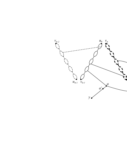
Figure 2: Schematic diagram of the choice of cutting bond. Solid lines represent $C_{n}$, dashed lines $C_{n-1}$, and bold dashed lines represent $\mathcal{B}_{n+1}$.

The first step in the second expansion is the identification of a suitable pivotal bond at which to sever the connection to $y$. We begin by applying Fubini’s theorem to interchange the $n^{{\rm th}}$ and $(n+1)^{{\rm st}}$ (bond/site) expectations, and regard the clusters $C_{n\pm 1}$ as being fixed. The occurrence of the events $(F_{1}^{\prime})_{l}$ on levels $l=n-1,n,n+1$ enforces a compatibility between $C_{n}$ and $C_{n\pm 1}$, in the sense that certain connections are required to occur for $C_{n}$. These connections are depicted schematically in Figure 2. We omit any discussion of the easier special cases where it is the expectation at level-0 or $N$ that is differentiated.

We recall the definition of the backbone of a cluster $C_{n+1}$ connecting $v_{n}$ to $u_{n+1}$, namely the set of all sites $x$ for which there are disjoint connections $x\longleftrightarrow v_{n}$ and $x\longleftrightarrow u_{n+1}$. We denote this backbone as $\mathcal{B}(C_{n+1})\equiv\mathcal{B}_{n+1}$. We also recall the existence of an ordering of the pivotal bonds for the connection from a site to a set of sites, as defined in Definition 2.1(d). The cutting bond is defined to be the last pivotal bond $(a^{\prime},a)$ for the connection $y\rightarrow\{v_{n-1},u_{n}\}\cup\mathcal{B}_{n+1}$. It is possible that no such pivotal bond exists, and in that case, no expansion is required.

In choosing the cutting bond, we require it to be pivotal for $\{v_{n-1},u_{n}\}$ to preserve (on the $a$ side of the cluster $C_{n}$) the backbone structure of the cluster $C_{n}$ which is required by $F_{1}^{\prime}(v_{n-1},u_{n};C_{n-1})_{n}$. Also, we require the cutting bond to be pivotal for $\mathcal{B}_{n+1}$ to ensure that we do not cut off as a tail something which may be needed to ensure that, as required by $F_{1}^{\prime}(v_{n},u_{n+1};C_{n})_{n+1}$, the last sausage of $C_{n+1}$ is connected through $C_{n}$.

Having chosen the cutting bond, we now begin to set the scene for the expansion. This requires an examination of the overall conditions present in the level-$n$ expectation. In addition to $F_{1}^{\prime}(v_{n-1},u_{n};C_{n-1})_{n}$ itself, there are conditions arising from $F_{1}^{\prime}(v_{n},u_{n+1};C_{n})_{n+1}$. The latter event can be decomposed as

$$F_{1}^{\prime}(v_{n},u_{n+1};C_{n})_{n+1}=F_{0}(v_{n},u_{n+1})_{n+1}\cap H_{\rm cut}(\mathcal{B}_{n+1})_{n},$$ (5.25)

where

$$F_{0}(v_{n},u_{n+1})_{n+1}= \left\{v_{n}\longleftrightarrow u_{n+1}\;\&\;v_{n}\longleftrightarrow{/}\hskip 7.74998ptG\right\}$$ (5.26)

$$H_{\rm cut}(\mathcal{B}_{n+1})_{n}= \Bigl{\{}C_{n}\textrm{ intersects }\mathcal{B}_{n+1}\textrm{ such that the level-$(n+1)$ connections satisfy}$$

$$(v_{n+1}^{\prime}\Longleftrightarrow u_{n+1}\textrm{ through }C_{n})\;\&\;(v_{n}\longleftrightarrow u_{n+1}^{\prime}\textnormal{ in }{{{\mathbb{Z}}}^{d}}\backslash C_{n})\Bigr{\}},$$ (5.27)

with $(u_{n+1}^{\prime},v_{n+1}^{\prime})$ the last pivotal bond for the level-$(n+1)$ connnection from $v_{n}$ to $u_{n+1}$ required by $(F_{1})_{n+1}$. (If there is no such pivotal bond, the requirements in (5.27) are replaced by $v_{n}\Longleftrightarrow u_{n+1}$ through $C_{n}$). Our task now is to rewrite the overall level-$n$ condition $F_{1}^{\prime}(v_{n-1},u_{n};C_{n-1})_{n}\cap H_{\rm cut}(\mathcal{B}_{n+1})_{n}\cap\left\{y\in C_{n}\right\}_{n}$ into a form suitable for generating the expansion.

Recall the definition of $\tilde{C}^{(a,a^{\prime})}(A)$ given in Definition 2.1. We define several events, as in Section 2.2. These events depend on $y,v_{n-1},u_{n},C_{n-1},\mathcal{B}_{n+1}$, but to simplify the notation we make only the $y$-dependence explicit in the notation. Let

$$H_{1}(y)_{n}=\, \left\{y\longleftrightarrow v_{n-1}\right\}\cap F_{1}^{\prime}(v_{n-1},u_{n};C_{n-1})_{n}\cap H_{\rm cut}(\mathcal{B}_{n+1})_{n},$$ (5.28)

$$H_{1}^{\prime}(y)_{n}=\, H_{1}(y)_{n}\cap\left\{y\Longleftrightarrow\{v_{n-1},u_{n}\}\cup\mathcal{B}_{n+1}\right\},$$ (5.29)

$$H_{1}^{\prime\prime}(a,a^{\prime})_{n}=\, \{H_{1}^{\prime}(a)_{n}\textnormal{ occurs on }\tilde{C}_{n}^{\{a,a^{\prime}\}}(\{v_{n-1},u_{n}\}\cup\mathcal{B}_{n+1})\},$$ (5.30)

$$H_{1}(a,a^{\prime},y)_{n}=\, H_{1}(y)_{n}\cap\left\{(a^{\prime},a)\textrm{ is the last occupied pivotal bond for }y\rightarrow\{v_{n-1},u_{n}\}\cup\mathcal{B}_{n+1}\right\}.$$ (5.31)

Then the overall level-$n$ event $H_{1}(y)_{n}$ is the disjoint union

$$H_{1}(y)_{n}=H_{1}^{\prime}(y)_{n}\bigcup^{\cdot}\biggl{(}\bigcup_{(a,a^{\prime})}^{\cdot}H_{1}(a,a^{\prime},y)_{n}\biggr{)}.$$ (5.32)

In (5.32), configurations in $H_{1}(y)_{n}$ have been classified according to the last pivotal bond $(a^{\prime},a)$. The appearance of $H_{1}^{\prime}$ corresponds to the possibility that there is no such pivotal bond, and in this case, no expansion will be required.

For the configurations in which there is a pivotal bond, we will use the following important lemma.

Lemma 5.3.

The events $H_{1}(a,a^{\prime},y)_{n}$ and $H_{1}^{\prime\prime}(a,a^{\prime})_{n}$ obey

$$H_{1}(a,a^{\prime},y)_{n}=\, H_{1}^{\prime\prime}(a,a^{\prime})_{n}\cap\left\{(y\longleftrightarrow a^{\prime}\;\&\;y\longleftrightarrow{/}\hskip 7.74998ptG)\textnormal{ occurs in }{{{\mathbb{Z}}}^{d}}\backslash\tilde{C}_{n}^{\{a,a^{\prime}\}}(\{v_{n-1},u_{n}\}\cup\mathcal{B}_{n+1})\right\}$$

$$\cap\left\{\{a,a^{\prime}\}\textnormal{ is occupied}\right\}.$$ (5.33)

Before proving the lemma, we note that together with (5.32) and Lemma 2.4 it implies the identity

$$\left\langle I[H_{1}(y)_{n}]\right\rangle_{n}^{\tilde{}}=\left\langle I[H_{1}^{\prime}(y)_{n}]\right\rangle_{n}^{\tilde{}}+p_{c}\sum_{(a,a^{\prime})}\langle I[H_{1}^{\prime\prime}(a,a^{\prime})_{n}]\,\tau_{h}^{\tilde{C}_{n}^{\{a,a^{\prime}\}}(\{v_{n-1},u_{n}\}\cup\mathcal{B}_{n+1})}(a^{\prime},y)\rangle_{n}^{\tilde{}}.$$ (5.34)

This will be the point of departure for the second expansion. Initially, the restricted two-point function appearing in the above equation should be with respect to the conditional, rather than the usual expectation. However, there is no difference between the two. To see this, note that the event that $a^{\prime}\longleftrightarrow y$ in ${{{\mathbb{Z}}}^{d}}\backslash\tilde{C}_{n}^{\{a,a^{\prime}\}}(\{v_{n-1},u_{n}\}\cup\mathcal{B}_{n+1})$ is independent of the bond $\{u_{n},v_{n}\}$, since this bond touches the set $\tilde{C}_{n}^{\{a,a^{\prime}\}}(\{v_{n-1},u_{n}\}\cup\mathcal{B}_{n+1})$. Therefore either expectation can be used for the restricted two-point function, and for simplicity, we will use the ordinary unconditional expectation.

Proof of Lemma 5.3. To abbreviate the notation, we write $A=\{v_{n-1},u_{n}\}\cup\mathcal{B}_{n+1}$, and define

$$F_{\rm piv}=\{(a^{\prime},a)\textrm{ is pivotal for }y\rightarrow A\}.$$ (5.35)

By definition of $H_{1}(a,a^{\prime},y)_{n}$,

$$H_{1}(a,a^{\prime},y)_{n}=\left\{\{a,a^{\prime}\}\textrm{ is occupied }\right\}\cap H_{1}(y)_{n}\cap\left\{a\Longleftrightarrow A\right\}\cap F_{\rm piv}.$$ (5.36)

We introduce the events

$$\mathcal{F}_{1} =\left\{a\longleftrightarrow v_{n-1}\right\}_{n}\cap\left\{a\Longleftrightarrow A\right\}_{n}\cap F_{1}^{\prime}(v_{n-1},u_{n};C_{n-1})_{n}\cap H_{\rm cut}(\mathcal{B}_{n+1})_{n},$$ (5.37)

$$\mathcal{F}_{2} =\left\{y\longleftrightarrow a^{\prime}\;\&\;y\longleftrightarrow{/}\hskip 7.74998ptG\right\}_{n},$$ (5.38)

and claim that

$$\begin{split}H_{1}(a,a^{\prime},y)_{n}&=\{\mathcal{F}_{1}\textnormal{ occurs on }\tilde{C}^{\{a,a^{\prime}\}}(A)\}\cap\{\mathcal{F}_{2}\textnormal{ occurs in }{{{\mathbb{Z}}}^{d}}\backslash\tilde{C}^{\{a,a^{\prime}\}}(A)\}\\ &\quad\cap\left\{\{a,a^{\prime}\}\textrm{ is occupied }\right\}\cap F_{\rm piv}.\end{split}$$ (5.39)

Assuming the claim, Lemma 2.5 can then be employed to rewrite the last event in the above, to give

$$H_{1}(a,a^{\prime},y)_{n} =\bigl{\{}(\mathcal{F}_{1}\;\&\;a\longleftrightarrow A)\textnormal{ occurs on }\tilde{C}^{\{a,a^{\prime}\}}(A)\bigr{\}}\cap\left\{\{a,a^{\prime}\}\textrm{ is occupied }\right\}$$

$$\quad\cap\bigl{\{}(\mathcal{F}_{2}\;\&\;y\longleftrightarrow a^{\prime})\textnormal{ occurs in }{{{\mathbb{Z}}}^{d}}\backslash\tilde{C}^{\{a,a^{\prime}\}}(A)\bigr{\}}.$$ (5.40)

In view of the definitions of $\mathcal{F}_{1}$ and $\mathcal{F}_{2}$, this implies the desired identity (5.33).

It remains to prove (5.39). Combining (5.36) and (5.28), we have

$$H_{1}(a,a^{\prime},y)_{n} =\left\{\{a,a^{\prime}\}\textrm{ is occupied }\right\}\cap\left\{y\longleftrightarrow v_{n-1}\right\}\cap F_{1}^{\prime}(v_{n-1},u_{n};C_{n-1})_{n}$$

$$\quad\cap H_{\rm cut}(\mathcal{B}_{n+1})_{n}\cap\left\{a\Longleftrightarrow A\right\}\cap F_{\rm piv}.$$ (5.41)

To see that this can be written in the form (5.39), we will analyze the various events in the above expression.

We begin with $\left\{y\longleftrightarrow v_{n-1}\right\}$, and note that

$$\left\{y\longleftrightarrow v_{n-1}\right\}\cap F_{\rm piv}$$ (5.42)

$$\hskip 28.45274pt=\left\{y\longleftrightarrow a^{\prime}\right\}\cap\left\{\{a,a^{\prime}\}\textrm{ is occupied }\right\}\cap\{a\longleftrightarrow v_{n-1}\textnormal{ occurs on }\tilde{C}^{\{a,a^{\prime}\}}(A)\}\cap F_{\rm piv}.$$

In fact, the right side is clearly contained in the left side. Conversely, for a configuration on the left side, since $v_{n-1}\in A$, the bond $(a^{\prime},a)$ must also be pivotal for $y\longleftrightarrow v_{n-1}$, and this implies that $\left\{y\longleftrightarrow a^{\prime}\right\}$, that $\{a^{\prime},a\}$ is occupied, and that $a\longleftrightarrow v\textnormal{ occurs on }\tilde{C}^{\{a,a^{\prime}\}}(v_{n-1})$. Since $\tilde{C}^{\{a,a^{\prime}\}}(v_{n-1})\subset\tilde{C}^{\{a,a^{\prime}\}}(A)$, this implies $\{a\longleftrightarrow v_{n-1}\textnormal{ occurs on }\tilde{C}^{\{a,a^{\prime}\}}(A)\}$. This proves (5.42). Now, by Lemma 2.5, $F_{\rm piv}$ is the intersection of the events $\{y\longleftrightarrow a^{\prime}\textnormal{ occurs in }{{{\mathbb{Z}}}^{d}}\backslash\tilde{C}^{\{a,a^{\prime}\}}(A)\}$ and $\{a\longleftrightarrow A\textnormal{ occurs on }\tilde{C}^{\{a,a^{\prime}\}}(A)\}$, and hence it follows from (5.42) that

$$\left\{y\longleftrightarrow v_{n-1}\right\}\cap F_{\rm piv} =\left\{\{a,a^{\prime}\}\textrm{ is occupied }\right\}\cap\{a\longleftrightarrow v_{n-1}\textnormal{ occurs on }\tilde{C}^{\{a,a^{\prime}\}}(A)\}$$

$$\quad\cap\{y\longleftrightarrow a^{\prime}\textnormal{ in }{{{\mathbb{Z}}}^{d}}\backslash\tilde{C}^{\{a,a^{\prime}\}}(A)\}.$$ (5.43)

Next we prove that

$$F_{1}^{\prime}(v_{n-1},u_{n};C_{n-1})_{n}\cap F_{\rm piv}\cap\left\{y\longleftrightarrow v_{n-1}\right\}\cap\left\{\{a,a^{\prime}\}\textnormal{ is occupied }\right\}$$

$$\hskip 28.45274pt=\left\{F_{1}^{\prime}(v_{n-1},u_{n};C_{n-1})\textnormal{ occurs on }\tilde{C}_{n}^{\{a,a^{\prime}\}}(A)\right\}\cap\left\{y\longleftrightarrow{/}\hskip 7.74998ptG\textnormal{ in }{{{\mathbb{Z}}}^{d}}\backslash\tilde{C}_{n}^{\{a,a^{\prime}\}}(A)\right\}$$

$$\hskip 42.67912pt\cap\{y\longleftrightarrow a^{\prime}\textnormal{ in }{{{\mathbb{Z}}}^{d}}\backslash\tilde{C}^{\{a,a^{\prime}\}}(A)\}\cap\{a\longleftrightarrow v_{n-1}\textnormal{ occurs on }\tilde{C}^{\{a,a^{\prime}\}}(A)\}$$

$$\hskip 42.67912pt\cap\left\{\{a,a^{\prime}\}\textnormal{ is occupied }\right\}.$$ (5.44)

As a first observation, we note that by (5.3), the second last line in the above can be replaced by $\{y\longleftrightarrow v_{n-1}\}\cap F_{\rm piv}$, and we will interpret the right side in this way. To prove (5.3), we begin by supposing we have a configuration in the left side. To show that it is in the right side, it suffices to show that the first two events on the right side must then occur. By the $G$-free condition in $F_{1}^{\prime}$, together with the fact that $y\in C(v_{n-1})$, it follows that $\{v_{n-1}\longleftrightarrow{/}\hskip 7.74998ptG\textnormal{ occurs on }\tilde{C}^{\{a,a^{\prime}\}}(A)\}$ and that $\{y\longleftrightarrow{/}\hskip 7.74998ptG\textnormal{ in }{{{\mathbb{Z}}}^{d}}\backslash\tilde{C}_{n}^{\{a,a^{\prime}\}}(A)\}$. As for the bond connections required by $F_{1}^{\prime}$, these are conditions on the backbone $\mathcal{B}_{n}$, which are independent of bonds not touching $\tilde{C}^{\{a,a^{\prime}\}}(A)$ since $F_{\rm piv}$ occurs. Thus these connections must occur on $\tilde{C}^{\{a,a^{\prime}\}}(A)$, and we have shown that the left side of (5.3) is contained in the right side. Conversely, given a configuration on the right side, we need to show that $F_{1}^{\prime}$ occurs. The necessary bond connections again occur since $F_{\rm piv}$ occurs. To see that, in addition, $v_{n-1}\longleftrightarrow{/}\hskip 7.74998ptG$, we note that when $\{y\longleftrightarrow v_{n-1}\}\cap F_{\rm piv}$ occurs, $C_{n}(v_{n-1})=\tilde{C}_{n}^{\{a,a^{\prime}\}}(a)\stackrel{{\scriptstyle\cdot}}{{\cup}}\tilde{C}_{n}^{\{a,a^{\prime}\}}(a^{\prime})$, where the union is disjoint. But for a configuration on the right side of (5.3), the two clusters forming this disjoint union must be $G$-free. This completes the proof of (5.3).

Turning now to $H_{\rm cut}(\mathcal{B}_{n+1})_{n}$, we claim that

$$H_{\rm cut}(\mathcal{B}_{n+1})_{n}\cap F_{\rm piv}=\{H_{\rm cut}(\mathcal{B}_{n+1})_{n}\textnormal{ occurs on }\tilde{C}^{\{a,a^{\prime}\}}(A)\}\cap F_{\rm piv}.$$ (5.45)

In fact, if the left side occurs, then the right side occurs because $F_{\rm piv}$ requires $(a^{\prime},a)$ to be pivotal for $y$’s connection to $\mathcal{B}_{n+1}$ and hence all $C_{n}$’s connections to $\mathcal{B}_{n+1}$ are independent of bonds not touching $\tilde{C}^{\{a,a^{\prime}\}}(A)$. Conversely, the right side is contained in the left side for the same reason.

Finally, we claim that

$$\left\{a\Longleftrightarrow A\right\}\cap F_{\rm piv}=\{a\Longleftrightarrow A\textnormal{ occurs on }\tilde{C}^{\{a,a^{\prime}\}}(A)\}\cap F_{\rm piv}.$$ (5.46)

In fact, because $\left\{a\Longleftrightarrow A\right\}$ is increasing, the right side is contained in the left side. Conversely, for a configuration on the left side, it must be the case that $\{a\Longleftrightarrow A\textnormal{ occurs on }\tilde{C}^{\{a,a^{\prime}\}}(a)\}$, and since $\tilde{C}^{\{a,a^{\prime}\}}(a)\subset\tilde{C}^{\{a,a^{\prime}\}}(A)$, the right side occurs.

The event $H_{1}(a,a^{\prime},y)_{n}$ is the intersection of the events occurring on the left sides of (5.3), (5.45) and (5.46). Therefore it is the intersection of the events occurring on the right sides of these equations. A rearrangement of these right side events then gives (5.39) and completes the proof. ∎

We are now in a position to obtain the identity (5.24), starting from (5.34) and using the one-$M$ scheme. With $N$ and $n$ fixed, the first step is to rewrite $\tau^{\tilde{C}}_{h}$ in (5.34) using (2.19). The result is

$$\left\langle I[H_{1}(y)_{n}]\right\rangle_{n}^{\tilde{}}= \left\langle I[H_{1}^{\prime}(y)_{n}]\right\rangle_{n}^{\tilde{}}+p_{c}\sum_{(a_{0},b_{0})}\left\langle I[H_{1}^{\prime\prime}(a_{0},b_{0})_{n}]\right\rangle_{n}^{\tilde{}}\,\tau_{h}(b_{0},y)$$

$$-p_{c}\sum_{(a_{0},b_{0})}\bigl{\langle}I[H_{1}^{\prime\prime}(a_{0},b_{0})_{n}]\langle I[F_{1}(b_{0},y;\tilde{C}_{n}^{\{a_{0},b_{0}\}}(\{v_{n-1},u_{n}\}\cup\mathcal{B}_{n+1}))\rangle_{(n,1)}\bigr{\rangle}_{n}^{\tilde{}}$$

$$+p_{c}\sum_{(a_{0},b_{0})}\bigl{\langle}I[H_{1}^{\prime\prime}(a_{0},b_{0})_{n}]\langle I[F_{2}(b_{0},y;\tilde{C}_{n}^{\{a_{0},b_{0}\}}(\{v_{n-1},u_{n}\}\cup\mathcal{B}_{n+1}))\rangle_{(n,1)}\bigr{\rangle}_{n}^{\tilde{}}.$$ (5.47)

We further expand the term containing $F_{1}$ using (2.31), leaving the term containing $F_{2}$ as it is. Let $\tilde{C}_{(n,0)}=\tilde{C}_{n}^{\{a_{0},b_{0}\}}(\{v_{n-1},u_{n}\}\cup\mathcal{B}_{n+1})$. For $j\geq 1$, let $\tilde{C}_{(n,j)}=\tilde{C}_{(n,j)}^{\{a_{j},b_{j}\}}(b_{j-1})$, $Z_{(n,j)}^{\prime}=I[F_{1}^{\prime}(b_{j-1},y;\tilde{C}_{(n,j-1)}]$, and $Z_{(n,j)}^{\prime}=I[F_{1}^{\prime\prime}(b_{j-1},a_{j},b_{j};\tilde{C}_{(n,j-1)}]$.

The first iteration can be written schematically as

$$\left\langle(H_{1})_{n}\right\rangle_{n}^{\tilde{}}= \left\langle(H_{1}^{\prime})_{n}\right\rangle_{n}^{\tilde{}}+\left\langle(H_{1}^{\prime\prime})_{n}\right\rangle_{n}^{\tilde{}}\,\tau-\left\langle(H_{1}^{\prime\prime})_{n}\langle(F_{1})_{(n,1)}\rangle_{(n,1)}\right\rangle_{n}^{\tilde{}}+\left\langle(H_{1}^{\prime\prime})_{n}\langle(F_{2})_{(n,1)}\rangle_{(n,1)}\right\rangle_{n}^{\tilde{}}$$

$$= \left\langle(H_{1}^{\prime})_{n}\right\rangle_{n}^{\tilde{}}+\left\langle(H_{1}^{\prime\prime})_{n}\right\rangle_{n}^{\tilde{}}\,\tau_{h}-\left\langle(H_{1}^{\prime\prime})_{n}\langle Z_{(n,1)}^{\prime}\rangle_{(n,1)}\right\rangle_{n}^{\tilde{}}-\left\langle(H_{1}^{\prime\prime})_{n}\langle Z_{(n,1)}^{\prime\prime}\rangle_{(n,1)}\right\rangle_{n}^{\tilde{}}\tau$$

$$+\left\langle(H_{1}^{\prime\prime})_{n}\left\langle Z^{\prime\prime}_{(n,1)}\langle(F_{1})_{(n,2)}\rangle_{(n,2)}\right\rangle_{(n,1)}\right\rangle_{n}^{\tilde{}}$$

$$+\left\langle(H_{1}^{\prime\prime})_{n}\langle(F_{2})_{(n,1)}\rangle_{(n,1)}\right\rangle_{n}^{\tilde{}}-\left\langle(H_{1}^{\prime\prime})_{n}\left\langle Z^{\prime\prime}_{(n,1)}\langle(F_{2})_{(n,2)}\rangle_{(n,2)}\right\rangle_{(n,1)}\right\rangle_{n}^{\tilde{}},$$ (5.48)

and we continue expanding the term containing $F_{1}$, to infinite order. The expansion to infinite order will be justified by the diagrammatic estimates of the next section. This leads to an identity that can be abbreviated as

$$\left\langle(H_{1})_{n}\right\rangle_{n}^{\tilde{}}=\hat{u}^{(n)}_{h}(0)+\hat{v}^{(n)}_{h}(0)\chi_{h}+\hat{e}^{(n)}_{h}(0),$$ (5.49)

where the first and second terms respectively comprise the terms with innermost expectation involving $Z^{\prime}$ and $Z^{\prime\prime}$, and the last term comprises those involving $F_{2}$. Explicitly,

$$\hat{v}_{h}^{(n)}(0) =\sum_{\ell=0}^{\infty}(-1)^{\ell}\hat{v}_{h}^{(n,\ell)}(0),\quad\quad\hat{v}_{h}^{(n,\ell)}(0)=\tilde{{\mathbb{E}}}_{n}(H_{1}^{\prime\prime})_{n}\,{{\mathbb{E}}}_{(n,1)}Z_{(n,1)}^{\prime\prime}\,\cdots{{\mathbb{E}}}_{(n,\ell)}Z_{(n,\ell)}^{\prime\prime}\,$$ (5.50)

$$\hat{e}_{h}^{(n)}(0) =\sum_{\ell=1}^{\infty}(-1)^{\ell}\hat{e}_{h}^{(n,\ell)}(0),\quad\quad\hat{e}_{h}^{(n,\ell)}(0)=\tilde{{\mathbb{E}}}_{n}(H_{1}^{\prime\prime})_{n}\,{{\mathbb{E}}}_{(n,1)}Z_{(n,1)}^{\prime\prime}\,\cdots{{\mathbb{E}}}_{(n,\ell-1)}Z_{(n,\ell-1)}^{\prime\prime}\,{{\mathbb{E}}}_{(n,\ell)}(F_{2})_{(n,\ell)},$$ (5.51)

and $\hat{u}_{h}^{(n)}(0)$ is defined as in (5.50) with $Z_{(n,\ell)}^{\prime}$ replacing $Z_{(n,\ell)}^{\prime\prime}$, and $H_{1}^{\prime}$ replacing $H_{1}^{\prime\prime}$ for $\ell=0$. In the $\ell=0$ term, only the leftmost expectation occurs.

Defining

$$\hat{\mathcal{V}}_{h}^{(N,n,\ell)}(0)={{\mathbb{E}}}_{0}I[E_{0}^{\prime\prime}]\,{{\mathbb{E}}}_{1}Y_{1}^{\prime\prime}\,\cdots{{\mathbb{E}}}_{n-1}Y_{n-1}^{\prime\prime}\,\tilde{{\mathbb{E}}}_{n+1}I[(F_{0})_{n+1}]\,\tilde{{\mathbb{E}}}_{n}\hat{v}^{(n,\ell)}_{h}(0)\,{{\mathbb{E}}}_{n+2}Y_{n+2}^{\prime\prime}\,\cdots{{\mathbb{E}}}_{N}Y_{N}^{\prime\prime},$$ (5.52)

this gives (5.24) with

$$\hat{\mathcal{V}}_{h}^{(N)}(0)=\sum_{n=0}^{N}\sum_{\ell=0}^{\infty}(-1)^{N}\hat{\mathcal{V}}_{h}^{(N,n,\ell)}(0)$$ (5.53)

and analogous expressions for $\hat{\mathcal{U}}^{(N)}_{h}(0)$ and $\hat{\mathcal{E}}^{(N)}_{h}(0)$. The right side of (5.52) requires special interpretation for the terms $n=0,N$.

5.4 Proof of Proposition 5.1

Proposition 5.1 follows from (5.24) and the following lemma. Section 5.4 is devoted to proving the lemma. The constant $K_{1}$ of Proposition 5.1 is given by $K_{1}=\hat{\mathcal{V}}_{0}(0)$, where $\hat{\mathcal{V}}_{0}(0)$ appears in the lemma.

Lemma 5.4.

The series $\hat{\mathcal{U}}_{h}(0)=\sum_{N=0}^{\infty}\hat{\mathcal{U}}_{h}^{(N)}(0)$, $\hat{\mathcal{V}}_{h}(0)=\sum_{N=0}^{\infty}\hat{\mathcal{V}}_{h}^{(N)}(0)$, and $\hat{\mathcal{E}}_{h}(0)=\sum_{N=0}^{\infty}\hat{\mathcal{E}}_{h}^{(N)}(0)$ converge absolutely. Moreover, $\hat{\mathcal{U}}_{h}(0)=O(1)$, $\hat{\mathcal{E}}_{h}(0)=o_{h}(1)\chi_{h}$, and

$$\hat{\mathcal{V}}_{h}(0)=\hat{\mathcal{V}}_{0}(0)+o_{h}(1),\qquad\hat{\mathcal{V}}_{0}(0)=1+O(\lambda).$$ (5.54)

Proof.   The analysis of $\hat{\mathcal{U}}_{h}(0)$ is almost identical to that of $\hat{\mathcal{V}}_{h}(0)$, so we discuss only $\hat{\mathcal{V}}_{h}(0)$ and $\hat{\mathcal{E}}_{h}(0)$. The proof consists of obtaining suitable diagrammatic estimates on $\hat{\mathcal{V}}_{h}^{(N,n,\ell)}(0)$ and $\hat{\mathcal{E}}_{h}^{(N,n,\ell)}(0)$ (see (5.52)). Roughly speaking, the bounds will involve horizontal “ladder” diagrams like those encountered in the bounds on $\hat{\Phi}_{h}(k)$, with an additional vertical ladder resulting from the nested expectation of $\hat{v}_{h}^{(n,\ell)}(0)$ or $\hat{e}_{h}^{(n,\ell)}(0)$. We will estimate these diagrams with the help of the power counting methodology of Appendix A.

We first consider the case $\ell=0$, and then move on to $\ell\geq 1$. Finally, we will prove (5.54).

The case $\ell=0$

There is no contribution to $\hat{\mathcal{E}}_{h}^{(N)}(0)$ arising from $\ell=0$, so we are concerned here with $\hat{\mathcal{V}}_{h}^{(N)}(0)$. Our goal is a diagrammatic estimate for

$$\hat{\mathcal{V}}_{h}^{(N,n,0)}(0)={{\mathbb{E}}}_{0}I[E_{0}^{\prime\prime}]\,{{\mathbb{E}}}_{1}Y_{1}^{\prime\prime}\,\cdots\tilde{{\mathbb{E}}}_{n-1}Y_{n-1}^{\prime}\,\tilde{{\mathbb{E}}}_{n+1}I[(F_{0})_{n+1}]\,\tilde{{\mathbb{E}}}_{n}(H_{1}^{\prime\prime})_{n}\,{{\mathbb{E}}}_{n+2}Y_{n+2}^{\prime\prime}\,\cdots{{\mathbb{E}}}_{N}Y_{N}^{\prime\prime}.$$ (5.55)

(We omit any discussion of the special cases $n=0,N$, which can be handled similarly.) This estimate will involve a modification of the diagrams used to estimate $\hat{\Phi}_{h}(0)$, obtained by “growing” a vertical diagram from the horizontal diagrams encountered in bounding $\hat{\Phi}_{h}(0)$.

We first note that, by (5.25) and (5.28)–(5.30), the intersection $(F_{0})_{n+1}\cap(H_{1}^{\prime\prime})_{n}$ is a subset of

$$\left\{a_{0}\longleftrightarrow v_{n-1}\right\}\cap\left\{a_{0}\Longleftrightarrow\{v_{n-1},u_{n}\}\cup\mathcal{B}_{n+1}\right\}\cap F_{1}^{\prime}(v_{n-1},u_{n};C_{n-1})_{n,b}\cap F_{1}^{\prime}(v_{n},u_{n+1};C_{n})_{n+1,b},$$ (5.56)

where the subscripts $b$ denote bond events with site conditions relaxed. Thus the bond connections that gave rise to the diagrammatic estimates on $\hat{\Phi}_{h}(k)$ in Section 3.2, due to $(F_{1}^{\prime})_{n,b}$ and $(F_{1}^{\prime})_{n+1,b}$, remain present after differentiation. The event

$$\left\{a_{0}\longleftrightarrow v_{n-1}\right\}\cap\left\{a_{0}\Longleftrightarrow\{v_{n-1},u_{n}\}\cup\mathcal{B}_{n+1}\right\}$$ (5.57)

provides additional connections that can be bounded using the BK inequality. In fact, (5.57) implies the existence of either (i) two disjoint level-$n$ paths $a_{0}\longleftrightarrow\{v_{n-1},u_{n}\}$, or (ii) disjoint level-$n$ paths $a_{0}\longleftrightarrow\{v_{n-1},u_{n}\}$ and $a_{0}\longleftrightarrow\mathcal{B}_{n+1}$. We now consider the diagrammatic implications of these two cases.

In case (i), the two connections implied by $a_{0}\Longleftrightarrow\{v_{n-1},u_{n}\}$ are added to the connections due to $(F_{1}^{\prime})_{n,b}$ that arise in the diagrams bounding this part of $\hat{\Phi}_{h}(k)$. This can be bounded, using the BK inequality, by adding two lines to the lines appearing already in the diagrammatic estimate for this part of $\hat{\Phi}_{h}(k)$ (the “old” lines), with the lines going from $a$ to two new vertices, say $c$ and $d$. Thus the resulting new diagrams are obtained by performing construction 1 followed by construction 2 of Section A.2 to the old diagrams. Examples of this construction are given in Figure 3 (a–b).

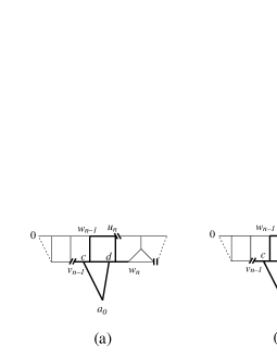
Figure 3: (a,b) Examples of diagrams arising from case (i). (c,d) An example of the diagrammatic bound of case (ii). Thick lines represent level-$n$ connections and thin lines represent levels-$(n\pm 1)$.

In case (ii), we add disjoint connections $a_{0}\longleftrightarrow\{v_{n-1},u_{n}\}$ and $a_{0}\longleftrightarrow\mathcal{B}_{n+1}$. We need only consider the case where the second of these paths is disjoint from the paths extracted from the event $(F_{1}^{\prime})_{n}$, because otherwise the situation reduces to case (i). For the path resulting from $a_{0}\longleftrightarrow\{v_{n-1},u_{n}\}$, we add a new vertex $c$ on an existing level-$n$ line of the $\Phi$ diagram, and then connect this vertex $c$ and $a_{0}$ with a new line. This takes care of the level-$n$ connection, and the situation is depicted in Figure 3 (c). For the second path, we must have a path from $a_{0}$ to some point $d$ in $\mathcal{B}_{n+1}$. We now have to ask how this $d$ is connected, via level-$(n+1)$ connections, to the rest of a level-$(n+1)$ diagram of $\Phi_{h}(k)$. For this purpose, we recall that $\mathcal{B}_{n+1}$ is the set of all points which are on a path from $v_{n}$ to $u_{n+1}$. As an upper bound, we just require $d\Longleftrightarrow\{v_{n},u_{n+1}\}$, which brings us back to the situation of case (i). Thus there are sites $e,f$ on the level-$(n+1)$ lines, with lines from $d$ to each of these sites. This is depicted in Figure 3 (d). The net result is an application of construction 1 (at $e$) followed by two applications of construction 2.

In summary, the resulting diagrams can be obtained by applying construction 1, followed by one or two applications of construction 2, to the diagrams used previously to bound $\hat{\Phi}_{h}(k)$, with the construction applied either at level-$n$ or on levels-$n$ and $n+1$. Now we bound these diagrams, in several steps.

We begin by decomposing the diagrams as in Section 3.2, both from the side of level-$0$ and level-$N$. These estimates produce triangles, with corresponding factors of $\lambda$. The decomposition from level-$0$ stops at level-$(n-2)$, and that from level-$N$ stops at level-$(n+2)$, with levels $n-1$, $n$ and $n+1$ remaining to be handled. A diagram corresponding to these levels will be open at its two ends, with a supremum over the displacement corresponding to the opening. This can be bounded above by the diagram obtained by closing the two ends and by closing the small openings corresponding to pivotal bonds. The possible results, before application of constructions 1 and 2, are depicted in Figure 4 (a), with the dashed lines representing the lines which are “moved” to close the diagram as an upper bound. There are eight possible combinations in all, with an example depicted in Figure 4 (b).

For the nearest-neighbour model in sufficiently high dimensions, we may employ squares, pentagons, etc. in our estimates, and it is not difficult to see that the diagrams obtained after applying constructions 1 and 2 are all $O(1)$. We therefore restrict attention now to the spread-out model. It can be checked that each of the eight diagrams can be obtained by applying construction 2 to the bubble, as depicted in Figure 4 (c). By Lemma A.3, for $d>6$, each of these diagrams therefore has infrared degree at least that of the bubble diagram, which has $\underline{\deg}_{0}=d-4$. Thus, by (A.14), the diagrams applied by a subsequent application of constructions 1 and 2 will have $\underline{\deg}_{0}\geq d-6>0$. By Theorem A.1, these diagrams are therefore convergent and $O(1)$.

In conclusion, we obtain the bound

$$|\hat{\mathcal{V}}_{h}^{(N,n,0)}(0)|\leq\min\{O(1),O(\lambda^{N-3})\}.$$ (5.58)

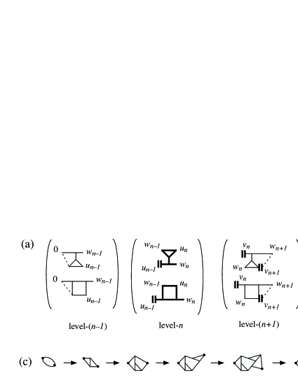
Figure 4: (a) The combinations producing the central diagram remaining after decomposition. (b) An example of a combination in (a). (c) Construction of the diagram in (b) via application of construction 2 to the bubble.

The case $\ell\geq 1$

We now consider the case $\ell\geq 1$, and obtain the bounds

$$|\hat{\mathcal{V}}_{h}^{(N,n,\ell)}(0)|\leq\min\{O(1),O(\lambda^{N+\ell-4})\},\quad\quad|\hat{\mathcal{E}}_{h}^{(N,n,\ell)}(0)|\leq\min\{O(1),O(\lambda^{N+\ell-4})\}o_{h}(1)\chi_{h}.$$ (5.59)

This is sufficient to prove Lemma 5.4, apart from (5.54) which we will prove later. The quantities on the left side of (5.59) will be bounded in terms of diagrams like those encountered above for $\ell=0$, but with further growth in the “vertical” direction. For $\mathcal{V}$, this vertical growth arises from additional expectations of $F_{1}^{\prime\prime}$, whereas for $\mathcal{E}$, the expectation at level-$(n,\ell)$ is $F_{2}^{\prime\prime}$. These modifications to the $\ell=0$ diagrams do not depend on levels $0$ to $n-2$ or on levels $n+2$ to $N$, and the expectations corresponding to these levels can be bounded by triangles as before to give rise to a factor $\lambda^{N-3}$ multiplied by a diagram with two ends closed as in the example shown in Figure 4 (b). Our task now is to understand the structure of this remaining diagram, with its vertical growth, and to bound it appropriately. We begin by considering the case $\ell=1$ of (5.59).

First, we consider $\hat{\mathcal{V}}_{h}^{(N,n,1)}(0)$. In view of (5.3)–(5.3), this requires estimation of

$$\bigl{\langle}I[H_{1}^{\prime\prime}(a_{0},b_{0})_{n}]\langle I[F_{1}^{\prime\prime}(b_{0},y;\tilde{C}_{n}^{\{a_{0},b_{0}\}}(\{v_{n-1},u_{n}\}\cup\mathcal{B}_{n+1}))\rangle_{(n,1)}\bigr{\rangle}_{n}^{\tilde{}}.$$ (5.60)

In a similar fashion to the case $\ell=0$ already treated, the $H_{1}^{\prime\prime}$ leads to application of constructions 1 and 2 applied to the $\hat{\Phi}_{h}(k)$-diagram reduced as in Figure 4 (b). This construction gives an infrared degree $\underline{\deg}_{0}\geq d-6>0$, as before. However, there are now additional new connections arising from $F_{1}^{\prime}$ in the level-$(n,1)$ expectation. These connections are as depicted in Figure 5 (a). They correspond to construction 3, which does not lower the infrared degree. It is not difficult to see that (5.60) is $O(1)$ for the nearest-neighbour model in sufficiently high dimensions. For the spread-out model, it is also $O(1)$, by power counting. This gives to an overall bound of order $\min\{1,\lambda^{N-3}\}$ for $\hat{\mathcal{V}}_{h}^{(N,n,1)}(0)$.

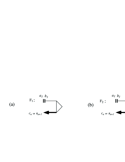
Figure 5: (a) The connections arising from level-$(n,1)$ in $\hat{\mathcal{V}}_{h}^{(N,n,1)}(0)$. (b) The connections arising from level-$(n,1)$ in $\hat{\mathcal{E}}_{h}^{(N,n,1)}(0)$.

Consider now $\hat{\mathcal{E}}_{h}^{(N,n,1)}(0)$, for which $F_{2}$ occurs on level-$(n,1)$. We first remove triangles as above, obtaining a factor of order $\min\{1,\lambda^{N-3}\}$. We then apply the cut-the-tail Lemma 3.5 in the usual way, extracting a factor $\chi_{h}$. The tail and remaining connections due to $F_{2}$ are depicted in Figure 5 (b). A factor $M_{h}$ arises from the connection to $G$, and the three remaining lines due to $F_{2}$ can be estimated by a factor of the triangle diagram. The remaining diagram is obtained from a diagram from the $\ell=0$ case by addition of a vertex on one of the lines corresponding to level-$n$ or level-$(n+1)$. For the nearest-neighbour model in sufficiently high dimensions, we may employ the square and larger diagrams and conclude an overall bound here of $O(1)M_{h}\chi_{h}=O(1)$. However, as we now explain, the spread-out model in dimensions $d>6$ requires more care.

Arguing as in Example 4.5, using Lemma 4.3 we may choose any one of the diagrammatic lines arising in any expectation other than level-$(n,1)$ to be $G$-free. We may therefore regard the additional vertex mentioned in the previous paragraph as residing on a massive line, with $\mu^{2}=\chi_{h}^{-1}$. Thus this extra vertex at worst reduces $\underline{\deg}_{0}$ by 2 to $d-8$ (according to Lemma A.3), but does not change $\underline{\deg}_{\mu}$. Hence the diagram is convergent for $h>0$, and by Theorem A.2, its rate of divergence as $h\rightarrow 0$ is bounded above by $O(\mu^{d-8}|\log\mu|^{L})=O(\chi_{h}^{(6-d)/2}|\log\chi_{h}|^{L})\chi_{h}=o_{h}(1)\chi_{h}$, consistent with (5.59).

Now we turn to the case $\ell\geq 2$, beginning with $\hat{\mathcal{V}}_{h}^{(N,n,\ell)}(0)$. Again we bound the expectations corresponding to levels-0 to $n-2$ and $n+2$ to $N$ by triangles, and close up the ends of the resulting diagram. Each expectation from levels-$(n,1)$ to $(n,\ell)$ corresponds diagrammatically to construction 2 applied to the diagrams encountered for the case $\ell=0$, and does not decrease the infrared degree. We may estimate each of these expectations with a triangle (each providing a factor $\lambda$), leaving a bounded diagram. This gives the desired bound for $\hat{\mathcal{V}}_{h}^{(N,n,\ell)}(0)$. For $\hat{\mathcal{E}}_{h}^{(N,n,\ell)}(0)$, we combine the method used for $\hat{\mathcal{V}}_{h}^{(N,n,\ell)}(0)$ with that employed for $\hat{\mathcal{E}}_{h}^{(N,n,1)}(0)$.

Proof of (5.54)

First we consider $\hat{\mathcal{V}}_{h}-\hat{\mathcal{V}}_{0}$. As we have seen, diagrams contributing to $\hat{\mathcal{V}}_{h}(0)$ are finite. As in (3.59), the difference gives rise to a connection to $G$. This is bounded pointwise by $M_{h}$, and hence the dominated convergence theorem can be applied to conclude that $\hat{\mathcal{V}}_{h}(0)-\hat{\mathcal{V}}_{0}(0)=o_{h}(1)$.

Finally, we argue that $\hat{\mathcal{V}}_{0}(0)=1+O(\lambda)$. Consider first the nearest-neighbour model. Using the square and higher diagrams if necessary, we can bound $\sum_{N,n,\ell}\hat{\mathcal{V}}_{h}^{(N,n,\ell)}(0)$ by $O(\lambda)$ for all terms except $N=n=\ell=0$. This can be seen from the fact that these terms all include at least one expectation having a pivotal bond, and the occurrence of a pivotal bond implies a bound $O(\lambda)$. The remaining term is the first term of (5.18). In that term, the contribution due to $u_{0}=0$ is readily seen to be $1+O(\lambda)$, while the contribution due to $u_{0}\neq 0$ is $O(\lambda)$. This gives the desired result for the nearest-neighbour model.

For the spread-out model, we argue similarly. However, in this case there are contributions from diagrams that we are unable to bound using a factor of the triangle that is clearly $O(\lambda)$. We have used power counting, previously, to bound these contributions by $O(1)$. To improve these bounds to $O(\lambda)$, we appeal to dominated convergence via the following argument (similar to [16, Lemma 5.9]). First we observe that by [16, (5.36)], if $k\neq 0$ then $\lim_{L\rightarrow\infty}1-\hat{D}(k)=1$. It follows that the limit of any convergent diagram containing summation over a pivotal bond $\{u,v\}$ is the corresponding integral of $e^{ik\cdot(v-u)}$, integrated over $[-\pi,\pi]^{d}$. This integral is zero. Since all the diagrams that were bounded using power counting do contain such a pivotal bond, we obtain the desired bound $O(\lambda)$.

∎

5.5 Differentiation of $\hat{\Xi}_{h}(0)$

In this section, we discuss the second expansion used in the proof of Proposition 5.2. Our analysis of $\hat{\Xi}_{h}(0)$ has much in common with the above analysis of $\hat{\Phi}_{h}(0)$, but there are also important differences. For $\hat{\Phi}_{h}(0)$, we used the fact that all connections involved in the definition of $\hat{\Phi}_{h}(0)$ were $G$-free to show that its derivative gave rise to a “tail” corresponding, after a second expansion to cut off the tail, to a factor of $\chi_{h}$. Integration of this factor of $\chi_{h}$ then gave rise to the $M_{h}$ appearing in (5.6). For $\hat{\Xi}_{h}(0)$, on the other hand, there is a connection to $G$ explicitly demanded in the expectation containing $W^{\prime}$. Although this easily gives rise to a bound involving $M_{h}$, we need to extract a factor of the magnetization in an asymptotic relation. We do not have an expansion that can be used to “cut off” a factor of $M_{h}$, so we will differentiate in this expectation to convert this connection to $G$ to a $G$-free tail. This tail can then be cut off, as a factor of the susceptibility, by means of a second expansion.

By the fundamental theorem of calculus, $\hat{\Xi}_{h}^{(n,m)}(0)$ can be written as

$$\hat{\Xi}_{h}^{(n,m)}(0) = (-1)^{m+n-1}\int_{0}^{h}du{{\mathbb{E}}}_{0,h}I[E_{0}^{\prime\prime}]{{\mathbb{E}}}_{1,h}Y_{1}^{\prime\prime}\cdots\tilde{{\mathbb{E}}}_{n-1,h}Y_{n-1}^{\prime}\frac{d}{du}\tilde{{\mathbb{E}}}_{n,u}W_{n}^{\prime}$$ (5.61)

$$\hskip 79.66771pt\times\;\tilde{{\mathbb{E}}}_{n+1,h}Y_{n+1}^{\prime}{{\mathbb{E}}}_{n+2,h}Y_{n+2}^{\prime\prime}\cdots{{\mathbb{E}}}_{n+m,h}Y_{n+m}^{\prime\prime},$$

where subscripts indicate the value of the magnetic field for each expectation. The factor $W_{n}^{\prime}$ involves the events $F_{3}^{\prime}$ and $F_{5}^{\prime}$, which require a connection to $G$, while the factors $Y_{j}$ involve only $G$-free connections.

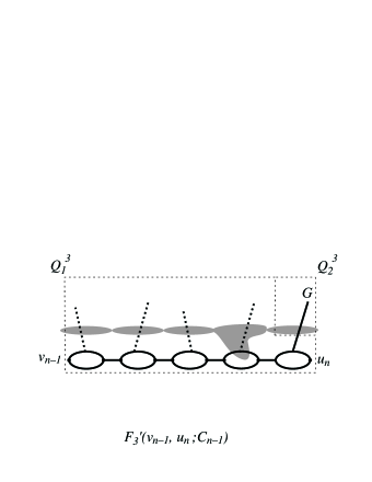
Figure 6: Schematic depiction of $Q^{3}_{1},Q^{3}_{2},Q^{5}_{1},Q^{5}_{2}$. Crosshatched regions represent $C_{n-1}$ and dotted lines represent possible but not mandatory connections in $C(v_{n-1})$.

To understand the derivative here, we introduce the clusters $Q^{j}_{1},Q^{j}_{2}$ ($j=3,5$) depicted in Figure 6. Explicitly, these are defined in conjunction with the occurrence of the event $F_{j}^{\prime}(v_{n-1},u_{n};\tilde{C}_{n-1})$, as follows:

$$Q^{3}_{2} = \{y\in\mbox{ last sausage of }{C}(v_{n-1}):u_{n}\stackrel{{\scriptstyle{C}_{n-1}}}{{\longleftrightarrow}}y\},$$

$$Q^{3}_{1} = C(v_{n-1})\backslash Q^{3}_{2},$$

$$Q^{5}_{2} = \{y\in{C}(v_{n-1})\backslash[\mbox{last sausage of }{C}(v_{n-1})]:v_{n-1}\stackrel{{\scriptstyle{C}_{n-1}}}{{\longleftrightarrow}}y\},$$

$$Q^{5}_{1} = C(v_{n-1})\backslash Q^{5}_{2}.$$

The $u$-dependence of $F_{3}^{\prime}$ and $F_{5}^{\prime}$ is then given by

$$e^{-u|Q^{j}_{1}|}\,(1-e^{-u|Q^{j}_{2}|})\quad(j=3,5).$$ (5.62)

Its derivative is

$$-|Q^{j}_{1}|e^{-u|Q^{j}_{1}|}\,(1-e^{-u|Q^{j}_{2}|})+|Q^{j}_{2}|e^{-u(|Q^{j}_{1}|+|Q^{j}_{2}|)}.$$ (5.63)

The second term will turn out to be the main term, for both $j=3,5$. The first term will give rise to error terms that can be handled more easily, using bounds which we defer to Section 5.6. We divide these contributions as

$$\hat{\Xi}_{h}^{(n,m)}(0)=\int_{0}^{h}du\left(\hat{\mathcal{M}}_{h,u}^{(n,m)}(0)+\hat{\mathcal{N}}_{h,u}^{(n,m)}(0)\right),$$ (5.64)

where $\hat{\mathcal{M}}_{h,u}^{(n,m)}(0)$ comprises the main terms due to the second term of (5.63), and $\hat{\mathcal{N}}_{h,u}^{(n,m)}(0)$ contains the terms corresponding to the first term of (5.63). In the remainder of this section, we consider only $\hat{\mathcal{M}}_{h,u}^{(n,m)}(0)$, because this is the term for which we apply a second expansion.

We first discuss the contribution to $\hat{\mathcal{M}}_{h,u}^{(n,m)}(0)$ arising from the $j=3$ case of (5.63). The result of the differentiation is $u$-dependence of the form which corresponds to the cluster $C_{n}$ being entirely $G$-free. We write the prefactor $|Q^{3}_{2}|$ as $\sum_{y}I[y\in Q^{3}_{2}]$. Our goal is to use a second expansion to cut off the connection to $y$, as in Section 5.3.

As in Section 5.3, the first step is the identification of a suitable pivotal bond at which to sever the connection to $y$. Again we apply Fubini’s theorem to interchange the $n^{{\rm th}}$ and $(n+1)^{{\rm st}}$ (bond/site) expectations, and regard the clusters $C_{n\pm 1}$ as being fixed. The occurrence of the events $(F_{1}^{\prime})_{l}$, $l=n\pm 1$ and the event $(F_{3}^{\prime})_{n}$ enforces a compatibility between $C_{n}$ and $C_{n\pm 1}$, in the sense that certain connections are required to occur for $C_{n}$. These connections are depicted schematically in Figure 7. In particular, the site $y$ is in the last sausage for $v_{n-1}\longrightarrow u_{n}$, and is connected to $v_{n-1}$ and $u_{n}$ through $\tilde{C}_{n-1}$, since $y\in Q^{3}_{2}$.

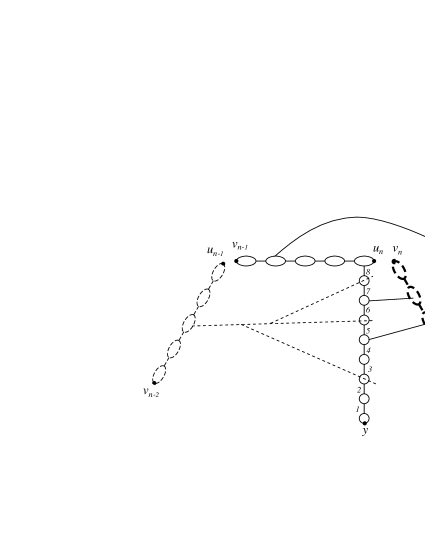
Figure 7: Schematic depiction of the choice of cutting bond for $F_{3}$. Solid lines represent $C_{n}$, dashed lines $C_{n-1}$, and bold dashed lines represent $\mathcal{B}_{n+1}$. Pivotal bonds in the last sausage are numbered 1 to 8. In this example, the cutting bond is bond 4.

To define the cutting bond, we let $\mathcal{P}(y)$ be the set of occupied pivotal bonds for $y\rightarrow u_{n}$, and given $b\in\mathcal{P}(y)$, we let $b_{+}$ be the endpoint of $b$ such that $u_{n}\in\tilde{C}_{n}^{b}(b_{+})$. We define the following two subsets of $\mathcal{P}(y)$:

$$\mathcal{P}_{n+1}(y) = \{b\in\mathcal{P}(y):b\textnormal{ is an occupied pivotal for }y\rightarrow\mathcal{B}_{n+1}\},$$

$$\mathcal{P}_{n-1}(y) = \{b\in\mathcal{P}(y):b_{+}\stackrel{{\scriptstyle{C}_{n-1}}}{{\longleftrightarrow}}u_{n}\}.$$

In Figure 7, $\mathcal{P}_{n+1}(y)=\{1,2,3,4\}$, while $\mathcal{P}_{n-1}(y)=\{1,2,3,4,5,6,7\}$. The cutting bond is then defined to be the last element of $\mathcal{P}_{n-1}(y)\cap\mathcal{P}_{n+1}(y)$, in the direction $y\rightarrow u_{n}$. In the example of Figure 7, the cutting bond is bond 4. It is possible that no such pivotal bond exists, and in that case, no expansion will be required.

The reason for the above choice for the cutting bond is as in Section 5.3. We require the cutting bond to be pivotal for $\mathcal{B}_{n+1}$ to ensure that we do not cut off as a tail something which may be needed to insure the intersection/avoidance properties between $C_{n}$ and $\mathcal{B}_{n+1}$ imposed by $(F_{3}^{\prime})_{n}$ and $(F_{1}^{\prime})_{n+1}$. We also want to maintain the connections through $C_{n-1}$ on the last sausage of $C_{n}$, and our choice does preserve these connections. This is analogous to the first expansion, where we cut at the first pivotal bond after the condition $v\stackrel{{\scriptstyle A}}{{\longleftrightarrow}}x$ has been satisfied.

Having chosen the cutting bond, we next examine the overall conditions present in the level-$n$ expectation. In addition to $F_{3}^{\prime}(v_{n-1},u_{n};C_{n-1})_{n}$ itself, there are conditions arising from the event $F_{1}^{\prime}(v_{n},u_{n+1};C_{n})_{n+1}$. Recalling the definitions in Section 5.3, the latter event can be decomposed as

$$F_{1}^{\prime}(v_{n},u_{n+1};C_{n})_{n+1}=F_{0}(v_{n},u_{n+1})_{n+1}\cap H_{\rm cut}(\mathcal{B}_{n+1})_{n}.$$ (5.65)

Our task now is to rewrite the overall level-$n$ condition $F_{3,b}^{\prime}(v_{n-1},u_{n};C_{n-1})_{n}\cap\{v_{n-1}\longleftrightarrow{/}\hskip 7.74998ptG\}_{n}\cap H_{\rm cut}(\mathcal{B}_{n+1})_{n}\cap\left\{y\in Q^{3}_{2}\right\}_{n}$ into a form suitable for generating the expansion. Here, $F_{3,b}^{\prime}(v_{n-1},u_{n};C_{n-1})_{n}$ denotes the intersection of $\{v_{n-1}\longleftrightarrow u_{n}\}$ with the event that the last sausage of $v_{n-1}\rightarrow u_{n}$ is connected to $C_{n-1}$.

As in Section 5.3, we define the events:

$$H_{3}(y)_{n}=\, \left\{y\in Q^{3}_{2}\right\}\cap F_{3,b}^{\prime}(v_{n-1},u_{n};C_{n-1})_{n}\cap\{v_{n-1}\longleftrightarrow{/}\hskip 7.74998ptG\}_{n}\cap H_{\rm cut}(\mathcal{B}_{n+1})_{n},$$ (5.66)

$$H_{3}^{\prime}(y)_{n}=\, H_{3}(y)_{n}\cap\left\{\mathcal{P}_{n-1}(y)\cap\mathcal{P}_{n+1}(y)=\emptyset\right\},$$ (5.67)

$$H_{3}^{\prime\prime}(a,a^{\prime})_{n}=\, \{H_{3}^{\prime}(a)_{n}\textnormal{ occurs on }\tilde{C}_{n}^{\{a,a^{\prime}\}}(\{v_{n-1},u_{n}\}\cup\mathcal{B}_{n+1})\},$$ (5.68)

$$H_{3}(a,a^{\prime},y)_{n}=\, H_{3}(y)_{n}\cap\left\{(a^{\prime},a)\textrm{ is the last occupied pivotal bond in }\mathcal{P}_{n-1}(y)\cap\mathcal{P}_{n+1}(y)\right\}.$$ (5.69)

Classifying configurations in $H_{3}(y)_{n}$ according to the last pivotal bond $(a,a^{\prime})$ (if there is one) yields the disjoint union

$$H_{3}(y)_{n}=H_{3}^{\prime}(y)_{n}\bigcup^{\cdot}\biggl{(}\bigcup_{(a,a^{\prime})}^{\cdot}H_{3}(a,a^{\prime},y)_{n}\biggr{)}.$$ (5.70)

For $H_{3}^{\prime}(y)_{n}$, no second expansion is required. For the configurations in which there is a pivotal bond, we will use the following lemma.

Lemma 5.5.

The events $H_{3}(a,a^{\prime},y)_{n}$ and $H_{3}^{\prime\prime}(a,a^{\prime})_{n}$ obey

$$H_{3}(a,a^{\prime},y)_{n}=\, H_{3}^{\prime\prime}(a,a^{\prime})_{n}\cap\left\{(y\longleftrightarrow a^{\prime}\;\&\;y\longleftrightarrow{/}\hskip 7.74998ptG)\textnormal{ occurs in }{{{\mathbb{Z}}}^{d}}\backslash\tilde{C}_{n}^{\{a,a^{\prime}\}}(\{v_{n-1},u_{n}\}\cup\mathcal{B}_{n+1})\right\}$$

$$\cap\left\{\{a,a^{\prime}\}\textnormal{ is occupied}\right\}.$$ (5.71)

We omit the proof of Lemma 5.5, since it proceeds in the same way as the proof of Lemma 5.3. However, there is one respect which is somewhat different. Unlike the analysis for $H_{1}(y)$, for $H_{3}^{\prime}$ it is not possible to write the “no pivotal” condition as $\{y\Longleftrightarrow C_{n-1}\cup\mathcal{B}_{n+1}\}$. It is true that every configuration in $H_{3}^{\prime}$ obeys $\{y\Longleftrightarrow C_{n-1}\cup\mathcal{B}_{n+1}\}$, but the converse is not true. For example, in the configuration of Figure 7, the true cutting bond is bond 4, even though $\{y\Longleftrightarrow C_{n-1}\cup\mathcal{B}_{n+1}\}$ occurs already after bond 2. But this difference from the situation in Lemma 5.3 is a minor one, and because our choice of the cutting bond imposes no $C_{n-1}$-related conditions on the $a^{\prime}$-side of the connection $y\longleftrightarrow a^{\prime}$, the analysis can proceed as before.

Now we note that together with (5.70) and Lemma 2.4, Lemma 5.5 implies the identity

$$\left\langle I[H_{3}(y)_{n}]\right\rangle_{n}^{\tilde{}}=\left\langle I[H_{3}^{\prime}(y)_{n}]\right\rangle_{n}^{\tilde{}}+p_{c}\sum_{(a,a^{\prime})}\langle I[H_{3}^{\prime\prime}(a,a^{\prime})_{n}]\,\tau_{u}^{\tilde{C}_{n}^{\{a,a^{\prime}\}}(\{v_{n-1},u_{n}\}\cup\mathcal{B}_{n+1})}(a^{\prime},y)\rangle_{n}^{\tilde{}}.$$ (5.72)

As in (5.34), the restricted two-point function in (5.72) is with respect to the ordinary unconditional expectation. The identity (5.72) is exactly analogous to (5.34), and the second expansion can be derived for (5.61) using the one-$M$ scheme, exactly as was done in Section 5.3. A minor difference here is that the level-$n$ expectation has magnetic field $u$. As a result, the expansion for the level-$n$ expectation is (5.3) with all the $H_{1}$ replaced by $H_{3}$, and with all the expectations of levels-$(n,m)$ having magnetic field $u$. Then we substitute this result back into (5.61). The result of the expansion will be given below, after we consider the case of $F_{5}$.

We now consider the main contribution to the $F_{5}$ case, which arises from the $j=5$ case of the seond term of (5.63). The choice of cutting bond is defined in exactly the same way as it was for the case of $F_{3}$, and the second expansion proceeds in the same way. We define $H_{5}$ events as in (5.66)–(5.68), with $F_{3}^{\prime}$ and $\{y\in Q^{3}_{2}\}$ in (5.66) respectively replaced by $F_{5}^{\prime}$ and $\{y\in Q^{5}_{2}\}$. This leads, as above, to the identity

$$\left\langle I[H_{5}(y)_{n}]\right\rangle_{n}^{\tilde{}}=\left\langle I[H_{5}^{\prime}(y)_{n}]\right\rangle_{n}^{\tilde{}}+p_{c}\sum_{(a,a^{\prime})}\langle I[H_{5}^{\prime\prime}(a,a^{\prime})_{n}]\,\tau_{u}^{\tilde{C}_{n}^{\{a,a^{\prime}\}}(\{v_{n-1},u_{n}\}\cup\mathcal{B}_{n+1})}(a^{\prime},y)\rangle_{n}^{\tilde{}}.$$ (5.73)

The second expansion then proceeds as usual, via the one-$M$ scheme. We perform the second expansion to infinite order, as will be justified by the bounds of the next section.

To summarize, the second expansion yields a result of the form

$$\hat{\mathcal{M}}_{h,u}^{(n,m)}(0)=\hat{\mathcal{G}}_{h,u}^{(n,m)}(0)+\hat{\mathcal{H}}_{h,u}^{(n,m)}(0)\chi_{u}+\hat{\mathcal{R}}_{h,u}^{(n,m)}(0).$$ (5.74)

The terms on the right side are sums of doubly nested expectations, with the second nesting occurring at level $n$ of the original nested expectation defining $\hat{\Xi}^{(n,m)}_{h}(0)$. The term $\hat{\mathcal{G}}_{h,u}^{(n,m)}(0)$ contains the terms in which the innermost expectation in the second nesting carries a single prime, and is analogous to $\mathcal{U}$ of (5.24). The term $\hat{\mathcal{H}}_{h,u}^{(n,m)}(0)$ contains the terms in which the innermost expectation in the second nesting carries a double prime, and is analogous to $\mathcal{V}$ of (5.24). The term $\hat{\mathcal{R}}_{h,u}^{(n,m)}(0)$ contains the terms in which the innermost expectation in the second nesting involves $F_{2}$, and is analogous to $\mathcal{E}$ of (5.24). Each of these three quantities can be written as a sum over $\ell$, where $\ell$ is the number of expectations nested within the $n^{\rm th}$ expectation.

5.6 Proof of Proposition 5.2

Lemma 5.6.

Let $u\in[0,h]$. The series $\hat{\mathcal{G}}_{h,u}(0)=\sum_{n,m=1}^{\infty}\hat{\mathcal{G}}_{h,u}^{(n,m)}(0)$, $\hat{\mathcal{H}}_{h,u}(0)=\sum_{n,m=1}^{\infty}\hat{\mathcal{H}}_{h,u}^{(n,m)}(0)$, $\hat{\mathcal{R}}_{h,u}(0)=\sum_{n,m=1}^{\infty}\hat{\mathcal{R}}_{h,u}^{(n,m)}(0)$, and $\hat{\mathcal{N}}_{h,u}(0)=\sum_{n,m=1}^{\infty}\hat{\mathcal{N}}_{h,u}^{(n,m)}(0)$ converge absolutely. Moreover, $\hat{\mathcal{G}}_{h,u}(0)=O(1)$, $\hat{\mathcal{R}}_{h,u}(0)=o_{h}(1)\chi_{u}$, $\hat{\mathcal{N}}_{h,u}(0)=o_{h}(1)\chi_{u}$, and

$$\hat{\mathcal{H}}_{h,u}(0)=\hat{\mathcal{H}}_{0,0}(0)+o_{h}(1),\quad\quad\hat{\mathcal{H}}_{0,0}(0)=O(\lambda).$$ (5.75)

Combining (5.64), (5.74), and Lemma 5.6, we have

$$\hat{\Xi}_{h}(0)=\int_{0}^{h}du\left(\hat{\mathcal{H}}_{0,0}(0)\chi_{u}+o_{h}(1)\chi_{u}\right)=\left(\hat{\mathcal{H}}_{0,0}(0)+o_{h}(1)\right)M_{h}.$$ (5.76)

This gives Proposition 5.2 with with $K_{2}=-\hat{\mathcal{H}}_{0,0}(0)$.

Proof of Lemma 5.6. The bounds on $\hat{\mathcal{G}}_{h,u}^{(n,m)}(0)$ are similar to those on $\hat{\mathcal{H}}_{h,u}^{(n,m)}(0)$, and will not be discussed further. Also, the arguments required for the nearest-neighbour and spread-out models are slightly different, as in the proof of Lemma 5.4, and for simplicity we restrict attention in what follows to the spread-out model.

Before beginning the proof in earnest, we examine the diagrams used to bound $\hat{\Xi}_{h}^{(n,m)}(0)$ in more detail. These differ from the diagrams of $\hat{\Phi}_{h}^{(n+m)}(0)$ only at levels $n-1,n,n+1$. When performing diagrammatic estimates, the other expectations can be bounded using triangles. These triangles give rise to a factor $\min\{1,\lambda^{n+m-3}\}$. Recalling (4.33)–(4.34) and Figure 4 (a), we are left with the truncated diagrams depicted schematically in Figure 8. The factor $\lambda^{n+m-3}$ controls the sums over $n,m$, and it suffices to obtain an appropriate bound on the truncated diagram, modified to take into account the diagrammatic changes arising in $\mathcal{N},\mathcal{H},\mathcal{R}$.

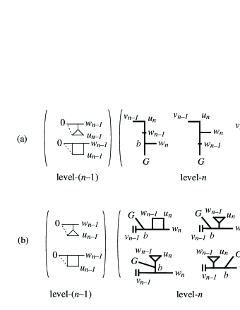
Figure 8: The truncated diagrams contributing to $\Xi$ due to (a) $F_{3}$ and (b) $F_{5}$.

It is helpful to examine the infrared degree of divergence of the diagrams of Figure 8. Consider first the diagrams of Figure 8 (a) with the line terminating at $G$ and the vertex at $b$ (for the first diagram) or $w_{n-1}$ (for the second and third diagrams) omitted, and those of Figure 8 (b) with the line terminating at $G$ and the vertex at $b$ omitted. We call these the amputated truncated diagrams. As in Figure 4 (c), it can be seen that the infrared degree of divergence of the amputated truncated diagrams is at least $d-4$. If we then restore the vertex at $w_{n-1}$ or $b$ to an amputated truncated diagram, this is construction 1 and hence the resulting diagram has infrared degree at least $d-6$, by Lemma A.3.

We divide the proof of Lemma 5.6 into several parts. First, we consider the error term $\mathcal{N}$. We then consider the $\ell=0$ contribution to $\mathcal{H}$. Then we move on to the contributions of $\ell\geq 1$ to $\mathcal{H}$ and $\mathcal{R}$. Finally, we prove (5.75). Our discussion will be brief at points where it does not differ substantially from the proof of Lemma 5.4.

Bounds on $\mathcal{N}$

The error term $\mathcal{N}$ is generated by the first term of (5.63), which involves adding a connection to $y\in Q_{1}^{3}$ or $y\in Q_{1}^{5}$, and then summing over $y$.

Consider first the case of an added connection to $y\in Q_{1}^{5}$. If we ignore the connection to $G$ in an upper bound, this corresponds to adding a vertex at level-$n$ to a truncated amputated diagram, with a line emanating to $y$. We can use the cut-the-tail Lemma 3.5 to extract a factor of $\chi_{u}$, multiplied by a diagram with infrared degree $d-6$. (This also involves an application of construction 2, which does not decrease the infrared degree.) However, if we recall that this diagram actually has a connection to $G$, we can use the dominated convergence theorem to obtain an overall bound $o_{h}(1)\chi_{u}$. The sum over $m,n$ can then be performed, thanks to the factor $\lambda^{n+m-3}$ mentioned previously.

Now consider the case of an added connection to $y\in Q_{1}^{3}$. In this case, the connection to $G$ plays an essential role in maintaining diagram connectivity, and it cannot be ignored. However, we can use Lemma 3.5 to produce a factor $\chi_{u}$, we can extract a factor $M_{u}$ from the connection to $G$, and by employing a $G$-free line from the expectation at level-$(n-1)$ or level-$(n+1)$ we can bound the remaining diagram by an analysis similar to that used to bound $\hat{\mathcal{E}}_{h}^{(N,n,1)}(0)$ in Section 5.4. The overall result is a bound $\chi_{u}M_{u}h^{(d-8)/4}\leq o_{h}(1)\chi_{u}$.

The case $\ell=0$

We now bound the diagrams contributing to the lowest order ($\ell=0$) contributions to $\mathcal{H}$, i.e.,

$${{\mathbb{E}}}_{0}I[E_{0}^{\prime\prime}]\,{{\mathbb{E}}}_{1}Y_{1}^{\prime\prime}\,\cdots\tilde{{\mathbb{E}}}_{n-1}Y_{n-1}^{\prime}\,\tilde{{\mathbb{E}}}_{n+1}I[(F_{0})_{n+1}]\,\tilde{{\mathbb{E}}}_{n}(H_{j}^{\prime\prime})_{n}\,{{\mathbb{E}}}_{n+2}Y_{n+2}^{\prime\prime}\,\cdots{{\mathbb{E}}}_{n+m}Y_{n+m}^{\prime\prime},$$ (5.77)

where $j=3$ or $j=5$. The discussion parallels the corresponding part of the proof of Lemma 5.4. The diagram is truncated as described above, and we bound the modification of the amputated truncated diagram which takes into account the additional connections implied by $H_{j}^{\prime\prime}$. We will argue that these connections arise from application of construction 1 followed by constructions 2 or 3. Thus the infrared degree of divergence is reduced from at least $d-4$ to at worst $d-6$, by (A.13)–(A.14), and hence the diagrams are $O(1)$.

Consider first the case $j=3$. In addition to the bond connections required by $F_{3}^{\prime}(v_{n-1},u_{n};C_{n-1})$, we add connections due to $a_{0}\in Q^{3}_{2}$ and $\mathcal{P}_{n-1}(a_{0})\cap\mathcal{P}_{n+1}(a_{0})=\emptyset$. The site $a_{0}$ is located in the place of $G$ of Figure 8 (a). By definition, it is either the case that $\mathcal{P}_{n-1}(a_{0})\subset\mathcal{P}_{n+1}(a_{0})$ or $\mathcal{P}_{n+1}(a_{0})\subset\mathcal{P}_{n-1}(a_{0})$. Thus we need only consider the two cases (i) $\mathcal{P}_{n-1}(a_{0})=\emptyset$ and (ii) $\mathcal{P}_{n+1}(a_{0})=\emptyset$.

We first consider case (i). This is depicted in Figure 9 (a). The extra required (disjoint) connections are $a_{0}\longleftrightarrow w_{n-1}$ and $a_{0}\longleftrightarrow b$. Here $b$ is a new vertex, while $w_{n-1}$ was existing. Thus this is an application of construction 2, which does not reduce the infrared degree. (A similar construction can be applied in the case where the connection to $w_{n}$ emerges from the sausage containing $w_{n-1}$.)

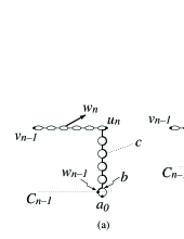
Figure 9: Original configurations for $\Xi$ ($F_{3}$ case), and new connections required for $a_{0}$.

We next consider case (ii). There are several geometries to consider, three of which are depicted in Figure 9 (b-d). In (b) and (c), there are additional disjoint paths from an existing vertex $b$ in the $\Xi$-diagram to $a_{0}$ (in (b), we take $b=w_{n-1}$) and from $a_{0}$ to a new vertex $c\in\mathcal{B}_{n+1}$. We may then argue as we did in the proof of Lemma 5.4 that $c$ is then connected to existing diagram lines from level-$(n+1)$ in such a way that the overall additional lines are of the form of construction 3. The geometry of Figure 9 (d), in which the connection to $w_{n}$ emerges from the sausage of $a_{0}$, deserves special comment. In this case, we may neglect any additional connection to $\mathcal{B}_{n+1}$ beyond that already present due to the connection from $b$ to $w_{n}$. The new lines to be added are those from $b$ to $a_{0}$ and from $a_{0}$ to $d$ (new), which is an application of construction 2.

Next, we move on to the case $j=5$ in (5.77), which involves $Q_{2}^{5}$ shown schematically in Figure 6.

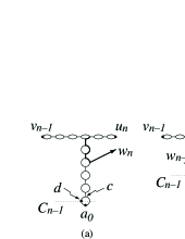
Figure 10: Original configurations for $\Xi$ ($F_{5}$ case), and new connections required for $a_{0}$.

Four of the relevant geometries are depicted in Figure 10. In (a), the new connections link $a_{0}$ to $d$ (existing) and $a_{0}$ to $c$ (new), which is construction 2. In (b), the new connections link $a_{0}$ to $w_{n-1}$ and $a_{0}$ to $d$ (new), which is construction 3. In (c), the new connections link $a_{0}$ to $c$ (existing) and $a_{0}$ to $d$ (new), which is construction 3. Finally, in (d), the new connections link $a_{0}$ to $c$ (existing) and $a_{0}$ to $d$ (new), which is construction 2. None of these constructions decrease the infrared degree from its original value of $d-6$, so the diagrams are $O(1)$.

The case $\ell\geq 1$

This case is bounded exactly as was done in the proof of Lemma 5.4. Note that we require massive lines to estimate $\mathcal{R}$, but after differentiation the level-$n$ expectation becomes $G$-free and the massive lines can be obtained as before. One new ingredient here is that we have two magnetic fields $h$ and $u$, but the simple inequalities $u\leq h$, $M_{u}\leq M_{h}$, and $\chi_{u}\geq\chi_{h}$ can be applied.

Proof of (5.75)

The proof that $\hat{\mathcal{H}}_{h,u}(0)=\hat{\mathcal{H}}_{0,0}(0)+o_{h}(1)$ proceeds as in the portion of the proof of Lemma 5.4 showing that $\hat{\mathcal{V}}_{h}(0)-\hat{\mathcal{V}}_{0}(0)=o_{h}(1)$, apart from the fact that now we have two magnetic fields $h$ and $u$. We again write the difference as a telescopic sum of differences at each level, and each difference implies a connection to $G$. We further decompose this sum of nested expectations as plus or minus sums of positive expectations. The difference can then be bounded above by setting $u=h$, since increasing the magnetic field increases the difference. Then our previous discussion applies.

To prove $\hat{\mathcal{H}}_{0,0}(0)=\lambda$, we use the dominated convergence theorem as in the proof that $\hat{\mathcal{V}}_{0}(0)=1+O(\lambda)$. However, each term in $\hat{\mathcal{H}}_{0,0}(0)$ contains at least one loop with a pivotal bond, and the $O(1)$ contribution does not occur. ∎

A Power counting for Feynman diagrams

In Section A.1, we summarize results of [27, 28] concerning the estimation of Feynman diagrams using the quantum field theoretic technique of power counting. Then in Section A.2, we provide a lemma which allows for an efficient application of these results for the Feynman diagrams arising in this paper.

A.1 Power counting

Consider a Feynman diagram $G$ consisting of $N$ internal lines, no external lines, and $V$ vertices. Each (internal) line carries a $d$-dimensional momentum $p_{i}$ ($i=1,2,\ldots,N$), and represents a propagator

$$\frac{1}{p_{i}^{2}+\mu_{i}^{2}},$$ (A.1)

where the mass $\mu_{i}$ of the $i^{\rm th}$ line can be either $0$ or $\mu>0$, with $\mu$ not depending on $i$. The massless ($\mu_{i}=0$) and massive $(\mu_{i}=\mu$) lines are fixed in $G$.

The Feynman diagrams encountered in this paper have propagator $\hat{\tau}_{h,p_{c}}(k)$. By Proposition 3.1, this propagator is bounded above by a constant multiple of $([1-\hat{D}(k)]+h^{1/2})^{-1}$, with the constant independent of $\Omega$. For both the nearest-neighbour and spread-out models, $1-\hat{D}(k)$ is bounded below by a universal constant multiple of $k^{2}/d$ (see [25, Appendix A]). Therefore $\hat{\tau}_{h,p_{c}}(k)$ is bounded above by a propagator of the form (A.1) times a factor $d$ which should be taken into account in bounding diagrams for the nearest-neighbour model, but which is unimportant for the spread-out model. Diagram lines with $h>0$ have mass $\mu=h^{1/4}$.

Each of the $V$ vertices of $G$ imposes a momentum conservation condition, according to Kirchoff’s law. Of these, $V-1$ are independent, with the momentum conservation at the other vertex then guaranteed by overall momentum conservation. As a result, we have $V-1$ independent momentum constraints. This leaves $L=N-V+1$ independent momenta $k_{j}$ ($j=1,2,\ldots,L$), called loop momenta, which can be chosen from $\{p_{i}\}_{i=1}^{N}$. The choice of loop momenta is not uniquely determined by $G$. Given a choice of loop momenta $\{k_{j}\}_{j=1}^{L}$, each $p_{i}$ can be written as a linear combination of the $k_{j}$. The Feynman integral $I_{G}$ giving the value of the Feynman diagram $G$ is then

$$I_{G}=\int_{[-\pi,\pi]^{d}}\frac{d^{d}k_{1}}{(2\pi)^{d}}\cdots\int_{[-\pi,\pi]^{d}}\frac{d^{d}k_{L}}{(2\pi)^{d}}\prod_{i=1}^{N}\frac{1}{p_{i}^{2}+\mu_{i}^{2}}.$$ (A.2)

The value of $I_{G}$ is independent of the choice of loop momenta.

Our goals are (i) to provide a sufficient condition for convergence of $I_{G}$ when $\mu\geq 0$, and (ii) to determine the rate of divergence of $I_{G}$, as $\mu\rightarrow 0$, in the case where $I_{G}$ is convergent for $\mu>0$ but not for $\mu=0$. For this, we will use the infrared degree of divergence $\underline{\deg}_{\mu}(G)$, which is defined as follows. First, given a set $\mathcal{G}$ of $L$ loop momenta, and a subset $\mathcal{H}\subset\mathcal{G}$ of cardinality $\ell$, we define the infrared degree of divergence of $\mathcal{H}$ by

$$\underline{\deg}_{\mu}(\mathcal{H})=d\ell-2\#\{\textrm{massless line momenta determined by $\mathcal{H}$}\}.$$ (A.3)

Note that (A.3) makes sense for $d\in{\mathbb{R}}$. For $\underline{\deg}_{0}$, all lines are regarded as massless, whereas for $\underline{\deg}_{\mu}$, only the lines for which $\mu_{i}=0$ are massless. In (A.3), a line momentum $p_{i}$ is said to be determined by $\mathcal{H}$ if $p_{i}$ is in the linear span of $\mathcal{H}$. Then we define the infrared degree of divergence of the full graph $G$ by

$$\underline{\deg}_{\mu}(G)=\min_{\mathcal{G}}\,\min_{\mathcal{H}:\mathcal{H}\subset\mathcal{G},\mathcal{H}\neq\emptyset}\,\underline{\deg}_{\mu}(\mathcal{H}),$$ (A.4)

where the minimum is taken over all choices $\mathcal{G}$ of loop momenta for $G$ and over all nonempty subsets $\mathcal{H}\subset\mathcal{G}$. The following theorem, which is [27, Theorem 1], asserts that a Feynman integral is finite if its infrared degree of divergence is positive.

Theorem A.1.

The Feynman integral $I_{G}$ converges if $\underline{\deg}_{\mu}(G)>0$.

Theorem A.1 implies that a diagram is more likely to be convergent in high dimensions. We define $d_{c}(G)$, the critical dimension of a diagram $G$, by

$$d_{c}(G)=\inf\{d\in{\mathbb{R}}:\underline{\deg}_{0}(G)>0\}.$$ (A.5)

By definition, $I_{G}$ converges if $d>d_{c}(G)$.

We now consider the situation where $I_{G}$ is convergent for $\mu>0$ but not for $\mu=0$. In this case, the following theorem, which we will show to be a consequence of [27, Theorem 2], indicates that the infrared degree of divergence $\underline{\deg}_{0}(G)$ bounds the rate of divergence of $I_{G}$ in the limit $\mu\rightarrow 0$.

Theorem A.2.

Suppose $\underline{\deg}_{\mu}(G)>0$ but $\underline{\deg}_{0}(G)\leq 0$. Then the Feynman integral $I_{G}$ is finite for $\mu>0$, and, as $\mu\rightarrow 0$, obeys the bound

$$I_{G}\leq\mbox{const.}\mu^{\underline{\deg}_{0}(G)}|\log\mu|^{L}.$$ (A.6)

Proof.   Making the change of variables $\tilde{k}_{i}=\mu^{-1}k_{i},\;\tilde{p}_{j}=\mu^{-1}p_{j}$ gives

$$I_{G}=\mu^{dL-2N}\int_{[-\pi/\mu,\pi/\mu]^{d}}\frac{d^{d}\tilde{k}_{1}}{(2\pi)^{d}}\cdots\int_{[-\pi/\mu,\pi/\mu]^{d}}\frac{d^{d}\tilde{k}_{L}}{(2\pi)^{d}}\prod_{i=1}^{N}\frac{1}{\tilde{p}_{i}^{2}+\tilde{\mu}_{i}^{2}}\equiv\mu^{dL-2N}J_{G},$$ (A.7)

where $\tilde{\mu}_{i}$ is zero or one, depending on whether $\mu_{i}$ is zero or $\mu$. The rate of divergence of $J_{G}$ is given in [27] in terms of the ultraviolet degree of divergence. This is defined as follows. Given a set of loop momenta $\mathcal{G}$ for $G$, and a subset $\mathcal{H}\subset\mathcal{G}$ of cardinality $\ell$, we define

$$\overline{\deg}(G)=\max_{\mathcal{G}}\max_{\mathcal{H}:\mathcal{H}\subset\mathcal{G},\mathcal{H}\neq\emptyset}\,\overline{\deg}(\mathcal{H}),\;\;\mbox{ where}\;\;\overline{\deg}(\mathcal{H})=d\ell-2\#\{\textrm{line momenta depending on $\mathcal{H}$}\}.$$ (A.8)

Here, a line momentum $p_{i}$ is said to be depending on $\mathcal{H}$ if it is not determined by $\mathcal{G}\backslash\mathcal{H}$. Also, since there is no mention of massless lines in the definition of the ultraviolet degree of divergence, there is no need to distinguish $\overline{\deg}_{\mu}$ and $\overline{\deg}_{0}$. It then follows from [27, Corollary to Theorem 2] that

$$J_{G}\leq\begin{cases}\textrm{const}.&(\overline{\deg}(G)<0)\\ \textrm{const}.\,\mu^{-\overline{\deg}(G)}|\log\mu|^{L}\quad&(\overline{\deg}(G)\geq 0).\end{cases}$$ (A.9)

Therefore

$$I_{G}\leq\mbox{const.}\mu^{dL-2N-\max\{0,\overline{\deg}(G)\}}|\log\mu|^{L}.$$ (A.10)

It remains to relate the exponent of $\mu$ on the right side to $\underline{\deg}_{0}(G)$. First, we claim that for any subset $\mathcal{H}\subset\mathcal{G}$,

$$\underline{\deg}_{0}(\mathcal{H})=dL-2N-\overline{\deg}(\mathcal{G}\backslash\mathcal{H}).$$ (A.11)

Here, we employ the convention $\underline{\deg}_{0}(\emptyset)=\overline{\deg}(\emptyset)=0$. The claim follows from the fact that the set $\mathcal{G}$ of all line momenta is the disjoint union of the set of line momenta determined by $\mathcal{H}$ and the set of line momenta depending on $\mathcal{G}\backslash\mathcal{H}$. Now, we take the minimum of (A.11) over all $\mathcal{G}$ and nonempty $\mathcal{H}\subset\mathcal{G}$. This leads to

$$\underline{\deg}_{0}(G) =dL-2N-\max_{\mathcal{G}}\max_{\mathcal{H}:\mathcal{H}\subset\mathcal{G},\mathcal{H}\neq\emptyset}\overline{\deg}(\mathcal{G}\backslash\mathcal{H})=dL-2N-\max_{\mathcal{G}}\max_{\mathcal{H}:\mathcal{H}\subset\mathcal{G},\mathcal{H}\neq\mathcal{G}}\overline{\deg}(\mathcal{H})$$

$$=dL-2N-\max\biggl{\{}0,\max_{\mathcal{G}}\max_{\mathcal{H}:\mathcal{H}\subset\mathcal{G};\mathcal{H}\neq\emptyset,\mathcal{G}}\overline{\deg}(\mathcal{H})\biggr{\}}.$$ (A.12)

We first consider the case where the maximum in the definition (A.8) of $\overline{\deg}(G)$ is attained at some $\mathcal{H}\neq\mathcal{G}$. Then (A.1) implies that $dL-2N-\max\{0,\overline{\deg}(G)\}=\underline{\deg}_{0}(G)$, and the bound of the theorem follows from (A.10).

This leaves the case where the maximum is attained at $\mathcal{H}=\mathcal{G}$, which implies $\overline{\deg}(G)=dL-2N$. Suppose first that $dL-2N<0$. Then we may include the case $\mathcal{H}=\mathcal{G}$ in the right side of (A.1) without changing its value, so again we have $dL-2N-\max\{0,\overline{\deg}(G)\}=\underline{\deg}_{0}(G)$ and the desired result follows from (A.10). Finally, suppose that $\overline{\deg}(G)=dL-2N\geq 0$. Relaxing the condition $\mathcal{H}\neq\mathcal{G}$ on the right side of (A.1) gives $\underline{\deg}_{0}(G)\geq dL-2N-\max\{0,\overline{\deg}(G)\}=dL-2N-(dL-2N)=0$. Since $\underline{\deg}_{0}(G)\leq 0$ by hypothesis, we may assume that $\underline{\deg}_{0}(G)=0$. The desired result then follows from (A.10), because the exponent of $\mu$ in (A.10) is zero (as we have just shown), and thus $I_{G}\leq\textrm{const}.\mu^{0}|\log\mu|^{L}=\textrm{const}.\mu^{\underline{\deg}_{0}(G)}|\log\mu|^{L}$. ∎

Theorems A.1 and A.2 reduce the analysis of Feynman integrals to the evaluation of the infrared degree of divergence. In the next section, we give a practical method for calculating the infrared degree of divergence of some of the Feynman diagrams arising in this paper.

A.2 Inductive power counting

Our goal in this section is to provide a lemma which allows the infrared degree of divergence of some of the Feynman diagrams appearing in this paper to be accurately estimated in terms of the infrared degree of divergence of related but simpler Feynman diagrams. This involves constructions in which a new Feynman diagram $G^{j}$ ($j=1,2,3$) is obtained from $G$ by the addition of new lines and/or vertices. These constructions are illustrated in Figure 11. The following lemma gives bounds on $\underline{\deg}(G^{j})$ in terms of $\underline{\deg}(G)$. In the lemma, either $\underline{\deg}_{\mu}(G)$ or $\underline{\deg}_{0}(G)$ can be used.

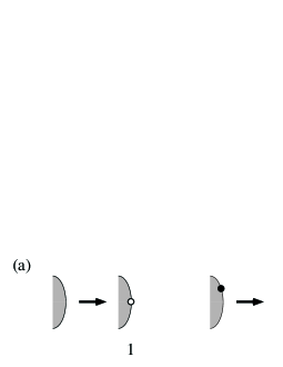
Figure 11: (a) A portion of $G$ is shown together with the corresponding portion of $G^{j}$ resulting from construction $j$. Solid dots denote vertices already present in $G$, while open dots denote new vertices, present in $G^{j}$ but not in $G$. Only those parts of $G$ which are changed are shown. (b) An example of construction 2 is depicted.

Lemma A.3.

The infrared degree of divergence of $G^{j}$ is bounded in terms of that of $G$ as follows:

$$\underline{\deg}(G^{j})\geq\begin{cases}\underline{\deg}(G)-2&(j=1)\\ \underline{\deg}(G)+\min\{0,d-6\}&(j=2).\end{cases}$$ (A.13)

Note that construction 3 results from two applications of construction 2, and hence

$$\underline{\deg}(G^{3})\geq\underline{\deg}(G)+2\min\{0,d-6\}.$$ (A.14)

Proof of Lemma A.3. We begin with the observation that, by definition, $\underline{\textnormal{deg}}(\mathcal{H})$ depends only on the subspace spanned by $\mathcal{H}$. Therefore, given $p^{\prime}{\not\in}\mathcal{H}$ with $p^{\prime}$ determined by $\mathcal{H}$, we can replace some vector $p\in\mathcal{H}$ by $p^{\prime}$ without changing $\underline{\textnormal{deg}}(\mathcal{H})$. This fact was called naturalness in [28].

Now we turn to the proof of (A.13) for Construction 1. In Construction 1, we add a new vertex to an existing line with momentum (say) $p_{1}$, thereby introducing a new line momentum $q_{1}$, as in Figure 12. Let $V$ be the number of vertices of $G$. The momentum conservation equations for $G$, which take the form $\sum_{j=1}^{N}\Lambda_{ij}p_{j}=0$ ($i=1,\ldots,V-1$) for some integers $\Lambda_{ij}$, are then supplemented with an additional equation $q_{1}=p_{1}$ for $G^{1}$. Choose $\mathcal{H}^{\prime}$ such that the minimum in the definition of $\underline{\textnormal{deg}}(G^{1})$ is attained at $\mathcal{H}^{\prime}$. Either $q_{1}$ is determined by $\mathcal{H}^{\prime}$ or it is not. If it is not, then $\mathcal{H}^{\prime}$ is a linearly independent subset of the $p_{j}$ obeying $\sum_{j=1}^{N}\Lambda_{ij}p_{j}=0$, and hence serves also as a subset $\mathcal{H}=\mathcal{H}^{\prime}$ of possible loop momenta for $G$. Therefore

$$\underline{\textnormal{deg}}(G^{1})=\underline{\textnormal{deg}}(\mathcal{H}^{\prime})=\underline{\textnormal{deg}}(\mathcal{H})\geq\underline{\textnormal{deg}}(G).$$ (A.15)

If, on the other hand, $q_{1}$ is determined by $\mathcal{H}^{\prime}$, then by naturalness, we may assume $p_{1}\in\mathcal{H}^{\prime}$ and $q_{1}{\not\in}\mathcal{H}^{\prime}$. Let $\mathcal{H}=\mathcal{H}^{\prime}$. Then $\mathcal{H}$ again serves as a subset of possible loop momenta for $G$. Since $\mathcal{H}$ determines one fewer line than $\mathcal{H}^{\prime}$ (due to the absence of $q_{1}$), we have

$$\underline{\textnormal{deg}}(G^{1})=\underline{\textnormal{deg}}(\mathcal{H}_{1}^{\prime})=\underline{\textnormal{deg}}(\mathcal{H})-2\geq\underline{\textnormal{deg}}(G)-2.$$ (A.16)

This completes the proof of (A.13) for Construction 1.

Next, we turn to the proof of (A.13) for Construction 2. Momenta before and after Construction 2 are labelled as in Figure 12. Suppose $G$ has $V$ vertices. The momentum conservation equations for $G$ can again be written as

$$\sum_{j=1}^{N}\Lambda_{ij}p_{j}=0\quad(i=1,\ldots,V-1).$$ (A.17)

For $G^{2}$, the corresponding equations can be written, for some integers $C_{i}$, in the form

$$\sum_{j=1}^{N}\Lambda_{ij}p_{j}=C_{i}q_{1}\quad(i=1,\ldots,V-1),\qquad q_{1}=q_{2},\qquad q_{3}=p_{2}+p_{3}.$$ (A.18)

The fact that the same coefficients $\Lambda_{ij}$ arise for $G$ and $G^{2}$ can easily be checked by comparing momentum conservation at vertices $a,b$ for $G$ with that at $a,b,c,d$ for $G^{2}$. Suppose the minimum in the definition of $\underline{\textnormal{deg}}(G^{2})$ is attained by $\mathcal{H}^{\prime}$. We again consider two cases, depending on whether $q_{1}$ is determined by $\mathcal{H}^{\prime}$ or not.

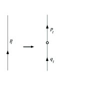
Figure 12: Constructions 1, 2 and labels of relevant momenta.

Suppose first that $q_{1}$ is determined by $\mathcal{H}^{\prime}$. By naturalness, we can assume $q_{1}\in\mathcal{H}^{\prime}$. Also, we can assume $q_{3}{\not\in}\mathcal{H}^{\prime}$, because if $q_{3}\in\mathcal{H}^{\prime}$ then $p_{1}$ is also determined (and would not be in $\mathcal{H}^{\prime}$ since $p_{1}=q_{1}+q_{3}$), and thus by naturalness, we can take $p_{1}$ rather than $q_{3}$ as a member of $\mathcal{H}^{\prime}$. We therefore assume that $q_{1}\in\mathcal{H}^{\prime}$ and $q_{3}{\not\in}\mathcal{H}^{\prime}$. Define $\mathcal{H}=\mathcal{H}^{\prime}\backslash\{q_{1}\}$. Since $\mathcal{H}^{\prime}$ is a set of loop momenta corresponding to the momentum constraints $\sum_{j=1}^{N}\Lambda_{ij}p_{j}=C_{i}q_{1}$, it follows that $\mathcal{H}$ is a set of loop momenta corresponding to $\sum_{j=1}^{N}\Lambda_{ij}p_{j}=0$, and hence is a subset of loop momenta for $G$. Comparing (A.17) and (A.18) shows that the number of $G$’s line momenta $p_{j}$ determined by $\mathcal{H}$ is the same as for $\mathcal{H}^{\prime}$. Since $\mathcal{H}$ has one fewer momentum than $\mathcal{H}^{\prime}$, and since there are at most three more lines determined by $\mathcal{H}^{\prime}$ than by $\mathcal{H}$ (namely $q_{1},q_{2},q_{3}$), we have

$$\underline{\textnormal{deg}}(G^{2})=\underline{\textnormal{deg}}(\mathcal{H}^{\prime})\geq\underline{\textnormal{deg}}(\mathcal{H})+d-6\geq\underline{\textnormal{deg}}(G)+d-6.$$ (A.19)

It remains to consider the case where $q_{1}$ is not determined by $\mathcal{H}^{\prime}$. In this case, at most one of the line momenta $p_{1}$ and $q_{3}$ is determined. However, the choice of labels $p_{1}$ and $q_{3}$ for these two lines was arbitrary, and we can and do choose the labelling that guarantees that the line momentum corresponding to $q_{3}$ is not determined. Since none of $q_{1},q_{2},q_{3}$ is determined, we have $q_{1},q_{2},q_{3}{\not\in}\mathcal{H}^{\prime}$. We now define $\mathcal{H}=\mathcal{H}^{\prime}$. It is conceivable that $\mathcal{H}$ may not be a subset of a set of line momenta for $G$, since independence of line momenta for $G^{2}$ (with its additional line momenta $q_{i}$) does not necessarily imply independence for $G$. To deal with this, we note that we can extend the definition (A.3) of $\underline{\textnormal{deg}}(\mathcal{H})$ also to dependent $\mathcal{H}$, and still maintain (A.4), because a dependent $\mathcal{H}$ will span a smaller space than an independent $\mathcal{H}$ consisting of the same number of vectors and hence cannot give the minimum in (A.4). Thus we have

$$\underline{\textnormal{deg}}(G^{2})=\underline{\rm deg}(\mathcal{H}^{\prime})\geq\underline{\rm deg}(\mathcal{H})\geq\underline{\textnormal{deg}}(G)$$ (A.20)

where the first inequality follows from the fact that $\mathcal{H}$ may determine more momenta in $G$ than in $G^{2}$ (since $q_{1}$ provides an additional degree of freedom in (A.18) compared to (A.17)), and the second inequality makes use of the extended definition of $\underline{\textnormal{deg}}(\mathcal{H})$ described above.

Combining (A.19) and (A.20) completes the proof of (A.13) for Construction 2, and the lemma is proved. ∎

References

- [1] M. Aizenman. The geometry of critical percolation and conformal invariance. In Hao Bai-Lin, editor, STATPHYS 19, Proceedings Xiamen 1995. World Scientific, (1996).
- [2] M. Aizenman. On the number of incipient spanning clusters. Nucl. Phys. B [FS], 485:551–582, (1997).
- [3] M. Aizenman. Scaling limit for the incipient spanning clusters. In K.M. Golden, G.R. Grimmett, R.D. James, G.W. Milton, and P.N. Sen, editors, Mathematics of Materials: Percolation and Composites. Springer, (1997).
- [4] M. Aizenman and A. Burchard. Hölder regularity and dimension bounds for random curves. Duke Math. J. To appear.
- [5] M. Aizenman and C.M. Newman. Tree graph inequalities and critical behavior in percolation models. J. Stat. Phys., 36:107–143, (1984).
- [6] D. Aldous. Tree-based models for random distribution of mass. J. Stat. Phys., 73:625–641, (1993).
- [7] D.J. Barsky and M. Aizenman. Percolation critical exponents under the triangle condition. Ann. Probab., 19:1520–1536, (1991).
- [8] C. Borgs, J.T. Chayes, R. van der Hofstad, and G. Slade. Mean-field lattice trees. Ann. Combinatorics. To appear.
- [9] J.T. Chayes, L. Chayes, and R. Durrett. Inhomogeneous percolation problems and incipient infinite clusters. J. Phys. A: Math. Gen., 20:1521–1530, (1987).
- [10] D. Dawson and E. Perkins. Measure-valued processes and renormalization of branching particle systems. In R. Carmona and B. Rozovskii, editors, Stochastic Partial Differential Equations: Six Perspectives. AMS Math. Surveys and Monographs, (1998).
- [11] E. Derbez and G. Slade. Lattice trees and super-Brownian motion. Canad. Math. Bull., 40:19–38, (1997).
- [12] E. Derbez and G. Slade. The scaling limit of lattice trees in high dimensions. Commun. Math. Phys., 193:69–104, (1998).
- [13] G. Grimmett. Percolation. Springer, Berlin, (1989).
- [14] T. Hara. Mean field critical behaviour for correlation length for percolation in high dimensions. Prob. Th. and Rel. Fields, 86:337–385, (1990).
- [15] T. Hara and G. Slade. The scaling limit of the incipient infinite cluster in high-dimensional percolation. II. Integrated super-Brownian excursion. Preprint.
- [16] T. Hara and G. Slade. Mean-field critical behaviour for percolation in high dimensions. Commun. Math. Phys., 128:333–391, (1990).
- [17] T. Hara and G. Slade. The number and size of branched polymers in high dimensions. J. Stat. Phys., 67:1009–1038, (1992).
- [18] T. Hara and G. Slade. Mean-field behaviour and the lace expansion. In G. Grimmett, editor, Probability and Phase Transition, Dordrecht, (1994). Kluwer.
- [19] T. Hara and G. Slade. The self-avoiding-walk and percolation critical points in high dimensions. Combinatorics, Probability and Computing, 4:197–215, (1995).
- [20] T. Hara and G. Slade. The incipient infinite cluster in high-dimensional percolation. Electron. Res. Announc. Amer. Math. Soc., 4:48–55, (1998). http:www.ams.orgera.
- [21] H. Kesten. The incipient infinite cluster in two-dimensional percolation. Probab. Th. Rel. Fields, 73:369–394, (1986).
- [22] J.-F. Le Gall. The uniform random tree in a Brownian excursion. Probab. Th. Rel. Fields, 96:369–383, (1993).
- [23] J.-F. Le Gall. Branching processes, random trees and superprocesses. In Proceedings of the International Congress of Mathematicians, Berlin 1998, volume III, pages 279–289, (1998). Documenta Mathematica, Extra Volume ICM 1998.
- [24] J.-F. Le Gall. The Hausdorff measure of the range of super-Brownian motion. In M. Bramson and R. Durrett, editors, Perplexing Problems in Probability: Papers in Honor of Harry Kesten, Basel, (1999). Birkhäuser.
- [25] N. Madras and G. Slade. The Self-Avoiding Walk. Birkhäuser, Boston, (1993).
- [26] B.G. Nguyen. Gap exponents for percolation processes with triangle condition. J. Stat. Phys., 49:235–243, (1987).
- [27] T. Reisz. A convergence theorem for lattice Feynman integrals with massless propagators. Commun. Math. Phys., 116:573–606, (1988).
- [28] T. Reisz. A power counting theorem for Feynman integrals on the lattice. Commun. Math. Phys., 116:81–126, (1988).
- [29] G. Slade. Lattice trees, percolation and super-Brownian motion. In M. Bramson and R. Durrett, editors, Perplexing Problems in Probability: Papers in Honor of Harry Kesten, Basel, (1999). Birkhäuser.
- [30] G. Toulouse. Perspectives from the theory of phase transitions. Nuovo Cimento, 23B:234–240, (1974).
- [31] W-S. Yang and Y. Zhang. A note on differentiability of the cluster density for independent percolation in high dimensions. J. Stat. Phys., 66:1123–1138, (1992).