Ribbon Graphs, Quadratic Differentials on Riemann Surfaces, and Algebraic Curves Defined over $\overline{\mathbb{Q}}$

Abstract.

It is well known that there is a bijective correspondence between metric ribbon graphs and compact Riemann surfaces with meromorphic Strebel differentials. In this article, it is proved that Grothendieck’s correspondence between dessins d’enfants and Belyi morphisms is a special case of this correspondence. For a metric ribbon graph with edge length $1$, an algebraic curve over $\overline{\mathbb{Q}}$ and a Strebel differential on it is constructed. It is also shown that the critical trajectories of the measured foliation that is determined by the Strebel differential recover the original metric ribbon graph. Conversely, for every Belyi morphism, a unique Strebel differential is constructed such that the critical leaves of the measured foliation it determines form a metric ribbon graph of edge length $1$, which coincides with the corresponding dessin d’enfant.

0. Introduction

In this article we give a self-contained explanation of the relation between ribbon graphs (combinatorial data), algebraic curves defined over $\overline{\mathbb{Q}}$ (algebraic and arithmetic data), and Strebel differentials on Riemann surfaces (analytic data).

For a given Riemann surface, we ask when it has the structure of an algebraic curve defined over the field $\overline{\mathbb{Q}}$ of algebraic numbers. A theorem of Belyi [1] answers this question saying that a nonsingular Riemann surface is an algebraic curve defined over $\overline{\mathbb{Q}}$ if and only if there is a holomorphic map of the Riemann surface onto $\mathbb{P}^{1}$ that is ramified only at $0$, $1$ and $\infty$. Such a map is called a Belyi map.

Grothendieck discovered that there is a natural bijection between the set of isomorphism classes of connected ribbon graphs and the set of isomorphism classes of Belyi maps. Thus a ribbon graph defines a Riemann surface with a complex structure and, moreover, its algebraic structure over $\overline{\mathbb{Q}}$. If we start with a Belyi map, then the corresponding ribbon graph is just the inverse image of the interval $[0,1]$ of $\mathbb{P}^{1}$. Grothendieck called these graphs Child’s Drawings (dessins d’enfants). We refer to [10] for more detail on this subject.

Another correspondence between ribbon graphs and Riemann surfaces, this time between metric ribbon graphs and arbitrary Riemann surfaces, has been known since the work of Harer, Mumford, Penner, Thurston, and others (see [3]). In this second correspondence, a ribbon graph arises as the union of critical leaves of a measured foliation defined on a Riemann surface by a meromorphic quadratic differential called a Strebel differential [2, 12]. When the Riemann surface is defined over $\overline{\mathbb{Q}}$, it coincides with the same surface that is given by the Grothendieck correspondence between ribbon graphs and algebraic curves defined over $\overline{\mathbb{Q}}$.

In this paper we give constructive proofs of these facts using canonical coordinate systems arising from Strebel differentials on a Riemann surface. The Child’s Drawings, Belyi maps and Strebel differentials are related in a very simple way, and they are explicitly described in terms of simple formulas.

Although these formulas could be written down in a few pages (see Section 6), for the sake of completeness we have included a detailed description of the theory which relates metric ribbon graphs and moduli spaces of Riemann surfaces with marked points.

In Section 1, we give a definition of ribbon graphs and their automorphisms. Thurston’s orbifolds and their Euler characteristics are defined in Section 2. With these preparations, in Section 3 we prove that the space of all isomorphism classes of metric ribbon graphs (i.e., ribbon graphs with a positive real number assigned to each edge) is a differentiable orbifold. Since a simplicial complex can be arbitrarily singular, this statement is not trivial. In Section 4, we review Strebel differentials on a Riemann surface, and construct a canonical coordinate system. The natural bijection between the space of metric ribbon graphs and the moduli space of Riemann surfaces with marked points is given in Section 5 by means of an explicit construction of the Strebel differential in terms of canonical coordinates corresponding to a metric ribbon graph. Finally, in Section 6, we give an explicit formula for the Belyi map corresponding to an arbitrary ribbon graph in terms of these canonical local coordinates.

The correspondence between metric ribbon graphs, quadratic differentials and the moduli space of Riemann surfaces is well-known to specialists. Moreover, formulas for these correspondences have appeared in the literature, in more or less explicit form. Nevertheless, the authors believe that our formulation of this correspondence is more precise, and leads to a simple formulation of some properties of algebraic curves defined over $\overline{\mathbb{Q}}$, which may be useful for further study.

Acknowledgement.

The authors thank Bill Thurston for explaining his work [11] to them. They are also grateful to Francesco Bottacin and Regina Parsons who has made valuable suggestions and improvements to the article. The work is partially supported by funding from the University of California, Davis, the University of Wisconsin, Eau Claire, and the NSF.

1. Ribbon graphs

A graph is a finite collection of points and line segments connected in certain ways, and a ribbon graph is a graph drawn on an oriented surface. A more careful definition of these objects is necessary when we consider their isomorphism classes.

Definition 1.1.

A graph $\Gamma=({\mathcal{V}},{\mathcal{E}},i)$ consists of a finite set ${\mathcal{V}}=\{V_{1},V_{2},\cdots,V_{v}\}$ of vertices and a finite set ${\mathcal{E}}$ of edges, together with a map $i$ from ${\mathcal{E}}$ to the set $({\mathcal{V}}\times{\mathcal{V}})/\mathfrak{S}_{2}$ of unordered pairs of vertices, called the incidence relation. An edge and a vertex are said to be incident if the vertex is in the image of the edge under $i$. The quantity

$$a_{jk}=|i^{-1}(V_{j},V_{k})|$$

gives the number of edges that connect two vertices $V_{j}$ and $V_{k}$. The degree, or valence, of a vertex $V_{j}$ is the number

$$\deg(V_{j})=\sum_{k\neq j}a_{jk}+2a_{jj},$$

which is the number of edges incident to the vertex. A loop, that is, an edge with only one incident vertex, contributes twice to the degree of its incident vertex. The degree of every vertex is required to be positive (no isolated vertices). The degree sequence of $\Gamma$ is the ordered list of degrees of the vertices:

$$(\deg(V_{1}),\deg(V_{2}),\cdots,\deg(V_{v})),$$

where the vertices are arranged so that the degree sequence is non-decreasing.

In this article, for the most part, we shall consider only graphs whose vertices all have degree at least $3$.

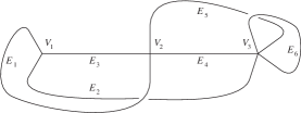
Figure 1.1. A graph consisting of $3$ vertices and $6$ edges.

Definition 1.2.

A traditional graph isomorphism $\phi=(\alpha,\beta)$ from a graph $\Gamma=({\mathcal{V}},{\mathcal{E}},i)$ to another graph $\Gamma^{\prime}=({\mathcal{V}}^{\prime},{\mathcal{E}}^{\prime},i^{\prime})$ is a pair of bijective maps

$$\alpha:{\mathcal{V}}\overset{\sim}{\longrightarrow}{\mathcal{V}}^{\prime}\qquad\text{and}\qquad\beta:{\mathcal{E}}\overset{\sim}{\longrightarrow}{\mathcal{E}}^{\prime}$$

that preserve the incidence relation, i.e., a diagram

(1.1) $$\begin{CD}{\mathcal{E}}@>{i}>{}>({\mathcal{V}}\times{\mathcal{V}})/\mathfrak{S}_{2}\\ @V{\beta}V{\wr}V@V{\wr}V{\alpha\times\alpha}V\\ {\mathcal{E}}^{\prime}@>{}>{i^{\prime}}>({\mathcal{V}}^{\prime}\times{\mathcal{V}}^{\prime})/\mathfrak{S}_{2}\end{CD}$$

commutes.

The traditional graph automorphism is not the natural notion when we consider graphs in the context of Riemann surfaces and Feynman diagram expansions. The reason is that the above definition of a graph does not distinguish between the half-edges, so that one cannot distinguish which vertex is associated to which half-edge, and thus the group of traditional group automorphisms is smaller than the automorphism group we will need to consider. One can treat the notion of graphs with distinguished half edges independently, but it is possible to embed the theory of such graphs within the ordinary definition of graphs by introducing the notion of the edge refinement of a graph $\Gamma=(\mathcal{V},\mathcal{E},i)$, which is the graph

$$\Gamma_{\mathcal{E}}=({\mathcal{V}}\coprod{\mathcal{V}}_{\mathcal{E}},{\mathcal{E}\coprod\mathcal{E}},i_{\mathcal{E}})$$

with the middle point of each edge of $\Gamma$ added as a degree 2 vertex, where ${\mathcal{V}}_{\mathcal{E}}$ denotes the set of all these midpoints of edges. The set of vertices of $\Gamma_{\mathcal{E}}$ is the disjoint union ${\mathcal{V}}\coprod{\mathcal{V}}_{\mathcal{E}}$, and the set of edges is the disjoint union ${\mathcal{E}}\coprod{\mathcal{E}}$ because the midpoint $V_{E}$ divides the edge $E$ into two parts. The incidence relation is described by a map

(1.2) $$i_{\mathcal{E}}:{\mathcal{E}}\coprod{\mathcal{E}}\longrightarrow{\mathcal{V}}\times{\mathcal{V}}_{\mathcal{E}},$$

because each edge of $\Gamma_{\mathcal{E}}$ connects exactly one vertex of ${\mathcal{V}}$ to a vertex of ${\mathcal{V}}_{\mathcal{E}}$. An edge of $\Gamma_{\mathcal{E}}$ is called a half-edge of $\Gamma$. For every vertex $V\in\mathcal{V}$ of $\Gamma$, the set $i_{\mathcal{E}}^{-1}(\{V\}\times\mathcal{V}_{\mathcal{E}})$ consists of half-edges incident to $V$. Note that we have

$$\deg(V)=|i_{\mathcal{E}}^{-1}(\{V\}\times{\mathcal{V}}_{\mathcal{E}})|.$$

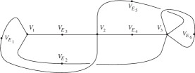
Figure 1.2. Edge refinement of the graph of Figure 1.1, with $9$ vertices and $12$ edges.

Definition 1.3.

Let $\Gamma=({\mathcal{V}},{\mathcal{E}},i)$ be a graph without vertices of degree less than $3$. The automorphism group ${\text{\rm{Aut}}}(\Gamma)$ is the group of traditional graph automorphisms of the edge refinement $\Gamma_{\mathcal{E}}$.

For example, the graph with one degree $4$ vertex and two edges has $(\mathbb{Z}/2\mathbb{Z})^{3}$ as its automorphism group, while the traditional graph automorphism group is just $\mathbb{Z}/2\mathbb{Z}$ (Figure 1.3).

Figure 1.3. A graph and its edge refinement.

Definition 1.4.

Let $\Gamma$ be a graph. Two edges $E_{1}$ and $E_{2}$ are connected if there is a vertex $V$ of $\Gamma$ such that both $E_{1}$ and $E_{2}$ are incident to $V$. A sequence of connected edges is an ordered set

(1.3) $$(E_{1},E_{2},\cdots,E_{k})$$

of edges of $\Gamma$ such that $E_{j}$ and $E_{j+1}$ are connected for every $j=1,2,\cdots,k-1$. A graph $\Gamma$ is connected if for every pair of vertices $V$ and $V^{\prime}$ of $\Gamma$, there is a sequence of connected edges (1.3) for some integer $k$ such that $E_{1}$ is incident to $V$ and $E_{k}$ is incident to $V^{\prime}$.

In this article we consider only connected graphs.

Definition 1.5.

A ribbon graph (or fatgraph) is a graph $\Gamma=({\mathcal{V}},{\mathcal{E}},i)$ together with a cyclic ordering on the set of half-edges incident to each vertex of $\Gamma$.

A ribbon graph can be represented on a positively oriented plane (i.e. a plane with counter-clockwise orientation) as a set of points corresponding to the vertices, connected by arcs for each edge between the points corresponding to its incident vertices, arranged so that the cyclic order of edges at a vertex corresponds to the orientation of the plane. Intersections of the arcs at points other than the vertices are ignored. The half edges incident to a vertex can be replaced with thin strips joined at the vertex, with the cyclic order at the vertex determining a direction on the boundaries of the strip (Figure 1.4).

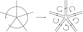
Figure 1.4. Oriented strips determined by the cyclic order at a vertex.

The strips corresponding to the two half edges are connected following the orientation of their boundaries to form ribbons, determining a figure which is no longer planar, but is an oriented surface with boundary given by the boundaries of the ribbons (Figure 1.5).

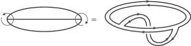
Figure 1.5. Oriented surface with boundary determined by a ribbon graph.

Thus a ribbon graph can be considered as an oriented surface with boundary, as is illustrated by Figure 1.6.

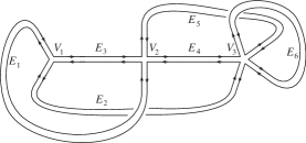
Figure 1.6. Ribbon graph of Figure 1.1 as an oriented surface.

Definition 1.6.

An automorphism of a ribbon graph $\Gamma$ is an automorphism of the underlying graph that preserves the cyclic ordering of half-edges at every vertex.

Since we deal mainly with ribbon graphs from now on, we use the notation ${\text{\rm{Aut}}}(\Gamma)$ for the automorphism group of a ribbon graph $\Gamma$. The characteristic difference between a graph and a ribbon graph is that the latter has a boundary.

Definition 1.7.

Let $\Gamma=({\mathcal{V}},{\mathcal{E}},i,c)$ be a ribbon graph, where $c$ denotes the cyclic ordering of half-edges at each vertex. A directed edge $\overrightarrow{E}$ is an ordering $E^{-}$ and $E^{+}$ of the half-edges that form the edge $E$. A boundary component(hole) of $\Gamma$ is a cyclic sequence of connected directed edges

$$(\overrightarrow{E_{0}},\overrightarrow{E_{1}},\cdots,\overrightarrow{E_{q-1}},\overrightarrow{E_{q}}=\overrightarrow{E_{0}})$$

such that the half-edges $E_{i}^{+}$ and $E_{i+1}^{-}$ are incident to a vertex $V_{i}$ of $\Gamma$, with $E_{i}^{+}$ immediately preceding $E_{i+1}^{-}$ with respect to the cyclic order assigned to the half-edges at $V_{i}$.

The ribbon graphs of Figure 1.5 and Figure 1.6 have only one boundary component. We denote by $b(\Gamma)$ the number of boundary components of a ribbon graph $\Gamma$.

Definition 1.8.

The group of ribbon graph automorphisms of $\Gamma$ that preserve the boundary components is denoted by ${\text{\rm{Aut}}}_{\partial}(\Gamma)$, which is a subgroup of ${\text{\rm{Aut}}}(\Gamma)$.

Since a boundary component of a ribbon graph is defined to be a cyclic sequence of directed edges, the topological realization of the ribbon graph has a well-defined orientation and each boundary component has an induced orientation that is compatible with the cyclic order. Thus we can attach an oriented disk to each boundary component of a ribbon graph $\Gamma$ so that the total space, which we denote by $C(\Gamma)$, is a compact oriented topological surface.

The attached disks and the underlying graph $\underline{\Gamma}$ of a ribbon graph $\Gamma$ defines a cell-decomposition of $C(\Gamma)$. Let $v(\Gamma)$ denote the number of vertices and $e(\Gamma)$ the number of edges of $\Gamma$. Then the genus $g(C(\Gamma))$ of the closed surface $C(\Gamma)$ is determined by a formula for the Euler characteristic:

(1.4) $$v(\Gamma)-e(\Gamma)+b(\Gamma)=2-2g(C(\Gamma)).$$

The ribbon graph of Figure 1.5 has two vertices, three edges and one boundary component. Thus the surface $C(\Gamma)$ is a torus.

Figure 1.7. Cell-decomposition of a torus by a graph drawn on it.

The ribbon graph of Figure 1.6 has three vertices, six edges and one boundary component. Thus the genus of the closed surface $C(\Gamma)$ associated with this ribbon graph is 2.

Figure 1.8. Cell-decomposition of a surface of genus $2$ by a ribbon graph.

In the next section we study metric ribbon graphs, which are ribbon graphs with a metric, that is, an assignment of a positive real number (length) to each edge of the graph. The set of all metrics on $\Gamma$ determines a topological space homeomorphic to $\mathbb{R}^{e(\Gamma)}_{+}$, on which the automorphism group of the ribbon graph acts. We wish to study the structure of the space of isomorphism classes of metrics under this action. A graph automorphism can act trivially on the space of metrics on $\Gamma$, and this happens precisely when the automorphism preserves the edges of $\Gamma$, but possibly interchanges some of its half-edges. Let us determine all ribbon graphs that have a non-trivial graph automorphism acting trivially on the set of edges.

Definition 1.9.

A ribbon graph $\Gamma$ is exceptional if the natural homomorphism

(1.5) $$\phi_{\Gamma}:{\text{\rm{Aut}}}(\Gamma)\longrightarrow\mathfrak{S}_{e(\Gamma)}$$

of the automorphism group of $\Gamma$ to the permutation group of edges is not injective.

Let $\Gamma$ be an exceptional graph and $\sigma\in{\text{\rm{Ker}}}(\phi_{\Gamma})$ a nontrivial automorphism of $\Gamma$. Since none of the edges are interchanged by $\sigma$, the graph can have at most two vertices. If the graph has two vertices, then $\sigma$ interchanges the vertices while all edges are fixed. The only possibility is a graph with two vertices of degree $j$, $(j\geq 3)$, as in Figure 1.5 and in Figure 1.9 below.

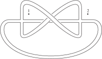
Figure 1.9. Exceptional graph type 1.

If $j$ is odd, then it has only one boundary component, as in Figure 1.5. The genus of the surface $C(\Gamma)$ is given by

(1.6) $$g(C(\Gamma))=\frac{j-1}{2}.$$

For an even $j$, the graph has two boundary components, as in Figure 1.9, and

(1.7) $$g(C(\Gamma))=\frac{j-2}{2}.$$

In both cases, the automorphism group is the product group

(1.8) $${\text{\rm{Aut}}}(\Gamma)=\mathbb{Z}/2\mathbb{Z}\times\mathbb{Z}/j\mathbb{Z},$$

with the factor $\mathbb{Z}/2\mathbb{Z}$ acting trivially on the set of edges.

When $\Gamma$ has two boundary components, then

$${\text{\rm{Aut}}}_{\partial}(\Gamma)=\mathbb{Z}/j\mathbb{Z},$$

which is a factor of (1.8). Note that ${\text{\rm{Aut}}}_{\partial}(\Gamma)$ acts faithfully on the set of edges in this case. Of course, in the case of one boundary component, ${\text{\rm{Aut}}}_{\partial}(\Gamma)$ coincides with ${\text{\rm{Aut}}}(\Gamma)$, so it does not act faithfully.

To obtain the one-vertex case, we only need to contract one of the edges of the two-vertex case considered above. The result is a graph with one vertex of degree $2k$, as shown in Figure 1.10.

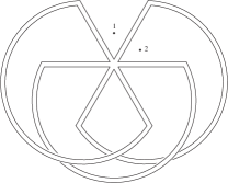
Figure 1.10. Exceptional graph type 2

When $k$ is even, the graph has only one boundary component, and the genus of the surface $C(\Gamma)$ is

(1.9) $$g(C(\Gamma))=\frac{k}{2}.$$

If $k$ is odd, then the graph has two boundary components and the genus is

(1.10) $$g(C(\Gamma))=\frac{k-1}{2}.$$

The automorphism group is $\mathbb{Z}/(2k)\mathbb{Z}$, but the action on $\mathbb{R}_{+}^{k}$ factors through

$$\mathbb{Z}/(2k)\mathbb{Z}\longrightarrow\mathbb{Z}/k\mathbb{Z}.$$

Here again, in the 2 component case the automorphism group fixing the boundary, ${\text{\rm{Aut}}}_{\partial}(\Gamma)=\mathbb{Z}/k\mathbb{Z}$, acts faithfully on the set of edges.

We have thus classified all exceptional graphs. These exceptional graphs appear for arbitrary genus $g$. The graph of Figure 1.9 has two distinct labelings of the boundary components, but since they can be interchanged by the action of a ribbon graph automorphism, there is only one equivalence class of ribbon graphs with labeled boundary over this underlying ribbon graph. The automorphism group that preserves the boundary is $\mathbb{Z}/4\mathbb{Z}$. Thus the space of metric ribbon graphs with labeled boundary is $\mathbb{R}_{+}^{4}/(\mathbb{Z}/4\mathbb{Z})$. The change of labeling, or the action of $\mathfrak{S}_{2}$, has a non-trivial effect on the graph level, but does not act at all on the space $\mathbb{R}_{+}^{4}/(\mathbb{Z}/4\mathbb{Z})$. The space of metric ribbon graphs is also $\mathbb{R}_{+}^{4}/(\mathbb{Z}/4\mathbb{Z})$, which is not the $\mathfrak{S}_{2}$-quotient of the space of metric ribbon graphs with labeled boundary.

The other example of an exceptional graph, Figure 1.10, gives another interesting case. This time the space of metric ribbon graphs with labeled boundary and the space of metric ribbon graphs without referring to the boundary are both $\mathbb{R}_{+}^{3}/(\mathbb{Z}/3\mathbb{Z})$. The group $\mathfrak{S}_{2}$ of changing the labels on the boundary has again no effect on the space.

The analysis of exceptional graphs shows that labeling all edges does not induce labeling of the boundary components of a ribbon graph. However, if we label all half-edges of a ribbon graph, then we have a labeling of the boundary components as well. We will come back to this point when we study the orbifold covering of the space of metric ribbon graphs by the space of metric ribbon graphs with labeled boundary components.

2. Orbifolds and the Euler Characteristic

A space obtained by patching pieces of the form

$$\frac{\text{smooth open ball}}{\text{finite group}}$$

together was called a $V$-manifold by Satake [9] and an orbifold by Thurston [13]. From the latter we cite:

Definition 2.1.

An orbifold $Q=\left(X(Q),\{U_{i}\}_{i\in I},\{G_{i}\}_{i\in I},\{\phi_{i}\}_{i\in I}\right)$ is a set of data consisting of

1. a Hausdorff topological space $X(Q)$ that is called the underlying space,

2. a locally finite open covering

   $$X(Q)=\bigcup_{i\in I}U_{i}$$

   of the underlying space,

3. a set of homeomorphisms

   $$\phi_{i}:U_{i}\overset{\sim}{\longrightarrow}\widetilde{U}_{i}/G_{i}.$$

   where $\widetilde{U}_{i}$ is an open subset of $\mathbb{R}^{n}$ and $G_{i}$ is a finite group acting faithfully on $\widetilde{U}_{i}$.

Whenever $U_{i}\subset U_{j}$, there is an injective group homomorphism

$$f_{ij}:G_{i}\longrightarrow G_{j}$$

and an embedding

$$\tilde{\phi}_{ij}:\widetilde{U}_{i}\longrightarrow\widetilde{U}_{j}$$

such that

$$\tilde{\phi}_{ij}(\gamma x)=f_{ij}(\gamma)\tilde{\phi}_{ij}(x)$$

for every $\gamma\in G_{i}$ and $x\in\widetilde{U}_{i}$, and such that the diagram below commutes.

$$\begin{CD}\widetilde{U}_{i}@>{\tilde{\phi}_{ij}}>{}>\widetilde{U}_{j}\\ @V{}V{}V@V{}V{}V\\ \widetilde{U}_{i}/G_{i}@>{\phi_{ij}=\tilde{\phi}_{ij}/G_{i}}>{}>\widetilde{U}_{j}/f_{ij}(G_{i})\\ \Big{\|}@V{}V{}V\\ \widetilde{U}_{i}/G_{i}@>{}>{}>\widetilde{U}_{j}/G_{j}\\ @A{\phi_{i}}A{\wr}A@A{\wr}A{\phi_{j}}A\\ U_{i}@>{\text{inclusion}}>{}>U_{j}.\end{CD}$$

The space $Q$ is called an orbifold locally modeled on $\mathbb{R}^{n}$ modulo finite groups. An orbifold is said to be differentiable if the group $G_{i}$ is a finite subgroup of the orthogonal group $O(n)$ acting on $\mathbb{R}^{n}$, and the local models $\mathbb{R}^{n}/G_{i}$ are glued together by diffeomorphisms.

Definition 2.2.

A surjective map

$$\pi:Q_{0}\longrightarrow Q_{1}$$

of an orbifold $Q_{0}$ onto $Q_{1}$ is said to be an orbifold covering if the following conditions are satisfied:

1. The map $\pi$ induces a surjective continuous map

   $$\pi:X(Q_{0})\longrightarrow X(Q_{1})$$

   between the underlying spaces, which is not generally a covering map of the topological spaces.

2. For every $x\in Q_{0}$, there is an open neighborhood $U\subset Q_{0}$, an open subset $\widetilde{U}\subset\mathbb{R}^{n}$, a finite group $G_{1}$ a subgroup $G_{0}\subset G_{1}$, and homeomorphisms $U\overset{\sim}{\longrightarrow}\widetilde{U}/G_{0}$ and $\pi(U)\overset{\sim}{\longrightarrow}\widetilde{U}/G_{1}$ such that the diagram below commutes.

   $$\begin{CD}U@>{\pi}>{}>\pi(U)\\ @V{\wr}V{}V@V{}V{\wr}V\\ \widetilde{U}/G_{0}@>{}>{}>\widetilde{U}/G_{1}\end{CD}$$

3. For every $y\in Q_{1}$, there is an open neighborhood $V$ of $y$, an open subset $\widetilde{V}\subset\mathbb{R}^{n}$, a finite group $G^{\prime}_{1}$, a subgroup $G^{\prime}_{0}\subset G^{\prime}_{1}$, and a connected component $U^{\prime}$ of $\pi^{-1}(V)$ making the diagram below commute.

   $$\begin{CD}U^{\prime}@>{\pi}>{}>V\\ @V{\wr}V{}V@V{}V{\wr}V\\ \widetilde{V}/G^{\prime}_{0}@>{}>{}>\widetilde{V}/G^{\prime}_{1}\end{CD}$$

If a group $G$ acts on a Riemannian manifold $M$ properly discontinuously by isometries, then

$$\pi:M\longrightarrow M/G$$

is an example of a differentiable covering orbifold.

Given point $x$ of an orbifold $Q$, there is a well-defined group $G_{x}$ associated to it. Let $U=\widetilde{U}/G$ be a local open coordinate neighborhood of $x\in Q$. Then the isotropy subgroup of $G$ that stabilizes any inverse image of $x$ in $U$ is unique up to conjugation. We define $G_{x}$ to be this isotropy group. When the isotropy group of $x$ is non-trivial, then $x$ is said to be a singular point of the orbifold. The set of non-singular points is open and dense in the underlying space $X(Q)$. An orbifold cell-decomposition of an orbifold is a cell-decomposition of $X(Q)$ such that the group $G_{x}$ is the same along each stratum. We denote by $G_{C}$ the group associated with a cell $C$.

Thurston extended the notion of the Euler characteristic to orbifolds.

Definition 2.3.

If an orbifold $Q$ admits an orbifold cell-decomposition, then we define the Euler characteristic by

(2.1) $${\hbox{\raise 1.5pt\hbox{$\chi$}}}(Q)=\sum_{C:\text{cell}}(-1)^{\text{dim}(C)}\frac{1}{|G_{C}|}.$$

The next theorem gives us a useful method to compute the Euler characteristic.

Theorem 2.4.

Let

$$\pi:Q_{0}\longrightarrow Q_{1}$$

be a covering orbifold. We define the sheet number of the covering $\pi$ to be the cardinality $k=|\pi^{-1}(y)|$ of the preimage $\pi^{-1}(y)$ of a non-singular point $y\in Q_{1}$. Then

(2.2) $${\hbox{\raise 1.5pt\hbox{$\chi$}}}(Q_{1})=\frac{1}{k}{\hbox{\raise 1.5pt\hbox{$\chi$}}}(Q_{0}).$$

Proof.

We first observe that for an arbitrary point $y$ of $Q_{1}$, we have

$$k=\sum_{x:\pi(x)=y}\frac{|G_{x}|}{|G_{y}|}.$$

Let

$$Q_{1}=\coprod_{j}C_{j}$$

be an orbifold cell-decomposition of $Q_{1}$, and

$$\pi^{-1}(C_{j})=\coprod_{i}C_{ij}$$

a division of the preimage of $C_{j}$ into its connected components. Then

$$\begin{split}k{\hbox{\raise 1.5pt\hbox{$\chi$}}}(Q_{1})&=k\sum_{j}(-1)^{\text{dim}(C_{j})}\frac{1}{|G_{C_{j}}|}\\ &=\sum_{j}(-1)^{\text{dim}(C_{j})}\sum_{i}\frac{|G_{C_{j}}|}{|G_{C_{ij}}|}\frac{1}{|G_{C_{j}}|}\\ &=\sum_{ij}(-1)^{\text{dim}(C_{ij})}\frac{1}{|G_{C_{ij}}|}\\ &={\hbox{\raise 1.5pt\hbox{$\chi$}}}(Q_{0}).\end{split}$$

∎

Corollary 2.5.

Let $G$ be a finite subgroup of $\mathfrak{S}_{n}$ that acts on $\mathbb{R}_{+}^{n}$ by permutation of the coordinate axes. Then $\mathbb{R}_{+}^{n}/G$ is a differentiable orbifold and

(2.3) $${\hbox{\raise 1.5pt\hbox{$\chi$}}}\left(\mathbb{R}_{+}^{n}/G\right)=\frac{(-1)^{n}}{|G|}.$$

Remark.

We note that in general

$${\hbox{\raise 1.5pt\hbox{$\chi$}}}\left(\mathbb{R}_{+}^{n}/G\right)\neq\frac{(-1)^{n}}{|G|},$$

unless $G$ acts on $\mathbb{R}_{+}^{n}$ faithfully.

Example 2.1.

Let us study the quotient space $\mathbb{R}_{+}^{n}/\mathfrak{S}_{n}$. We denote by

$$\Delta(123\cdots n)$$

the interior of a regular $n$-hyperhedron of $(n-1)$ dimensions. Thus $\Delta(12)$ is a line segment, $\Delta(123)$ is an equilateral triangle, and $\Delta(1234)$ is a regular tetrahedron. The space $\mathbb{R}_{+}^{n}$ is a cone over $\Delta(123\cdots n)$:

$$\mathbb{R}_{+}^{n}=\Delta(123\cdots n)\times\mathbb{R}_{+}.$$

The closure $\overline{\Delta(123\cdots n)}$ has $n$ vertices $x_{1},\cdots,x_{n}$. Let $x_{12}$ be the midpoint of the line segment $\overline{x_{1}x_{2}}$, $x_{123}$ the barycenter of the triangle $\triangle{x_{1}x_{2}x_{3}}$, etc., and $x_{123\cdots n}$ the barycenter of $\Delta(123\cdots n)$.

The $(n-1)$-dimensional region

(2.4) $$F=CH(x_{1},x_{12},x_{123},\cdots,x_{123\cdots n}),$$

which is the convex hull of the set of $n$ points $\{x_{1},x_{12},x_{123},\cdots,x_{123\cdots n}\}$, is the fundamental domain of the $\mathfrak{S}_{n}$-action on $\Delta(123\cdots n)$ induced by permutation of vertices. It can be considered as a cell complex of the orbifold $\mathbb{R}_{+}^{n}/\mathfrak{S}_{n}$. It has $\binom{n-1}{k}$ $k$-cells for every $k$ (Figure 2.1).

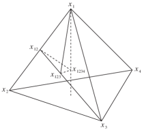
Figure 2.1. $\Delta(1234)$.

The isotropy group of each cell is easily calculated. For example, the isotropy group of the 2-cell $CH(x_{12}x_{123}x_{123\cdots n})$ is

$$\mathfrak{S}(12)\times\mathfrak{S}(456\cdots n),$$

where $\mathfrak{S}(abc\cdots z)$ is the permutation group of the specified letters. The definition of the Euler characteristic (2.1) and a computation using (2.2) gives an interesting combinatorial identity

(2.5) $$\begin{split}{\hbox{\raise 1.5pt\hbox{$\chi$}}}\left(\mathbb{R}_{+}^{n}/\mathfrak{S}_{n}\right)=&-{\hbox{\raise 1.5pt\hbox{$\chi$}}}\left(\Delta(123\cdots n)/\mathfrak{S}_{n}\right)\\ &=-\sum_{k=0}^{n-1}(-1)^{k}\sum_{\begin{subarray}{c}m_{0}+m_{1}+\cdots+m_{k}=n\\ m_{0}\geq 1,m_{1}\geq 1,\cdots,m_{k}\geq 1\end{subarray}}\frac{1}{m_{0}!m_{1}!\cdots m_{k}!}\\ &=\frac{(-1)^{n}}{n!}.\end{split}$$

The $\mathfrak{S}_{n}$-action of the cell-decomposition of

$$\Delta(123\cdots n)/\mathfrak{S}_{n}$$

gives a cell-decomposition of $\Delta(123\cdots n)$ itself, and hence a cell-decomposition of $\mathbb{R}_{+}^{n}$. We call this cell-decomposition the canonical cell-decomposition of $\mathbb{R}_{+}^{n}$, and denote it by $\square(\mathbb{R}_{+}^{n})$. For every subgroup $G\subset\mathfrak{S}_{n}$, the fixed point set of an element of $G$ is one of the cells of $\square(\mathbb{R}_{+}^{n})$. In particular, $\square(\mathbb{R}_{+}^{n})$ induces a cell-decomposition of the orbifold $\mathbb{R}_{+}^{n}/G$, which we call the canonical orbifold cell-decomposition of $\mathbb{R}_{+}^{n}/G$.

3. The Space of Metric Ribbon Graphs

The goal of this section is to show that the space of all metric ribbon graphs with fixed Euler characteristic and number of boundary components forms a differentiable orbifold. The metric ribbon graph space could a priori have complicated singularities, but it turns out that it only has quotient singularities given by certain finite group actions on Euclidean spaces of a fixed dimension. This is due to the behavior of the local deformations of a metric ribbon graph. The deformations of a metric ribbon graph which we will discuss below are related to certain questions in computer science. We refer to [11] for more detail.

Let $RG_{g,n}$ denote the set of all isomorphism classes of connected ribbon graphs $\Gamma$ with no vertices of degree less than $3$ such that

(3.1) $$\begin{cases}{\hbox{\raise 1.5pt\hbox{$\chi$}}}(\Gamma)=v(\Gamma)-e(\Gamma)=2-2g-n\\ b(\Gamma)=n,\end{cases}$$

where $v(\Gamma)$, $e(\Gamma)$ and $b(\Gamma)$ denote the number of vertices, edges and boundary components of $\Gamma$, respectively. If an edge $E$ of $\Gamma$ is incident to two distinct vertices $V_{1}$ and $V_{2}$, then we can construct another ribbon graph $\Gamma^{\prime}\in RG_{g,n}$ by removing the edge $E$ and joining the vertices $V_{1}$ and $V_{2}$ to a single vertex, with the cyclic order of the joined vertex determined by the cyclic order of the edges incident to $V_{1}$ starting from the edge following $E$ up to the edge preceding $E$, followed by the edges incident to $V_{2}$ starting with the edge following $E$ and ending with the edge preceding $E$. The ribbon graph $\Gamma^{\prime}$ is called a contraction of $\Gamma$. A partial ordering can be introduced into $RG_{g,n}$ by defining

(3.2) $$\Gamma_{2}\prec\Gamma_{1}$$

if $\Gamma_{2}$ is obtained by a series of contractions applied to $\Gamma_{1}$. Since contraction decreases the number of edges and vertices by one, a graph with only one vertex is a minimal graph, and a trivalent graph (a graph with only degree $3$ vertices) is a maximal element. Every graph can be obtained from a trivalent graph by applying a series of contractions.

The inverse operation to the contraction of a ribbon graph is expansion. Every vertex of degree $d\geq 4$ of a ribbon graph $\Gamma$ can be expanded by adding a new edge as shown in Figure 3.1.

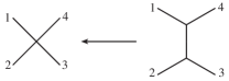
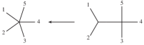
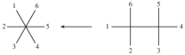
Figure 3.1. The arrow indicates contraction of an edge. The inverse direction is expansion of a vertex.

In the process of expansion of an ribbon graph $\Gamma$, we identify two expanded graphs if there is a ribbon graph isomorphism from one to the other that preserves all the original half-edges of $\Gamma$. Thus when we expand a vertex of degree $d\geq 4$, there are $d(d-3)/2$ ways of expanding it by adding an edge. The situation is easier to understand by looking at the dual graph of Figure 3.2, where the arrows again indicate the contraction map.

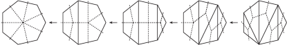
Figure 3.2. A series of expansions of a vertex of degree $7$ and the dual graphs.

Consider the portion of a ribbon graph consisting of a vertex of degree $d\geq 4$ and $d$ half-edges labeled by the numbers $1$ through $d$. We denote this portion by ${\ast_{d}}$. The dual graph of ${\ast_{d}}$ is a convex polygon with $d$ sides. The process of expansion by adding an edge to the center vertex of ${\ast_{d}}$ corresponds to drawing a diagonal line between two vertices of the $d$-gon, as in Figure 3.2. The number $d(d-3)/2$ corresponds to the number of diagonals in a convex $d$-gon. Expanding the graph further corresponds to adding another diagonal to the polygon in such a way that the added diagonal does not intersect with the existing diagonals except at the vertices of the polygon. The expansion process terminates after $d-3$ iterations, the number non-intersecting diagonals which can be placed in a convex $d$-gon. Note that such a maximal expansion is trivalent at the internal vertices, and its dual defines a triangulation of the polygon. The number of all triangulations of a $d$-gon is equal to

$$\frac{1}{d-1}\binom{2d-4}{d-2},$$

which is called the Catalan number.

A metric ribbon graph is a ribbon graph with a positive real number assigned to each edge, called the length of the edge. For a ribbon graph $\Gamma\in RG_{g,n}$, the space of isomorphism classes of metric ribbon graphs with $\Gamma$ as the underlying graph is a differentiable orbifold

(3.3) $$\frac{\mathbb{R}_{+}^{e(\Gamma)}}{{\text{\rm{Aut}}}(\Gamma)},$$

where the action of ${\text{\rm{Aut}}}(\Gamma)$ on $\mathbb{R}_{+}^{e(\Gamma)}$ is through the natural homomorphism

(3.4) $$\phi:{\text{\rm{Aut}}}(\Gamma)\longrightarrow\mathfrak{S}_{e(\Gamma)}.$$

For the exceptional graphs $\Gamma_{\rm{ex}}$ in Definition 1.9, we have

(3.5) $$\frac{\mathbb{R}_{+}^{e(\Gamma_{\rm{ex}})}}{{\text{\rm{Aut}}}(\Gamma_{\rm{ex}})}=\frac{\mathbb{R}_{+}^{e(\Gamma_{\rm{ex}})}}{{\text{\rm{Aut}}}(\Gamma)/(\mathbb{Z}/2\mathbb{Z})}.$$

For integers $g$ and $n$ satisfying

(3.6) $$\begin{cases}g\geq 0\\ n\geq 1\\ 2-2g-n<0,\end{cases}$$

we define the space of isomorphism classes of metric ribbon graphs satisfying the topological condition (3.1) by

(3.7) $$RG_{g,n}^{\text{met}}=\coprod_{\Gamma\in RG_{g,n}}\frac{\mathbb{R}_{+}^{e(\Gamma)}}{{\text{\rm{Aut}}}(\Gamma)}.$$

Each component (3.3) of (3.7) is called a rational cell of $RG_{g,n}^{\text{met}}$. The rational cells are glued together by the contraction operation in an obvious way. A rational cell has a natural quotient topology.

Let us compute the dimension of $RG_{g,n}^{\text{met}}$. We denote by $v_{j}(\Gamma)$ the number of vertices of a ribbon graph $\Gamma$ of degree $j$. Since these numbers satisfy

$$\begin{split}-(2-2g-n)&=-v(\Gamma)+e(\Gamma)\\ &=-\sum_{j\geq 3}v_{j}(\Gamma)+\frac{1}{2}\sum_{j\geq 3}jv_{j}(\Gamma)\\ &=\sum_{j\geq 3}\left(\frac{j}{2}-1\right)v_{j}(\Gamma),\end{split}$$

the number $e(\Gamma)$ of edges takes its maximum value when all vertices have degree $3$. In that case,

$$3v(\Gamma)=2e(\Gamma)$$

holds, and we have

(3.8) $$\dim(RG_{g,n}^{\text{met}})=\max_{\Gamma\in RG{g,n}}(e(\Gamma))=6g-6+3n.$$

To prove that $RG_{r,s}^{\rm{met}}$ is a differentiable orbifold, we need to show that for every element $\Gamma_{\rm{met}}\in RG_{r,s}^{\rm{met}}$, there is an open neighborhood $U_{\epsilon}(\Gamma_{\rm{met}})$ of $\Gamma_{\rm{met}}$, an open disk $\widetilde{U}_{\epsilon}(\Gamma_{\rm{met}})\subset\mathbb{R}^{6g-6+3n}$, and a finite group $G_{\Gamma}$ acting on $\widetilde{U}_{\epsilon}(\Gamma_{\rm{met}})$ through orthogonal transformations such that

$$\widetilde{U}_{\epsilon}(\Gamma_{\rm{met}})/G_{\Gamma}\cong U_{\epsilon}(\Gamma_{\rm{met}}).$$

Definition 3.1.

Let $\Gamma_{\rm{met}}\in RG_{g,n}^{\rm{met}}$ be a metric ribbon graph, and $\epsilon>0$ a positive number smaller than the half of the length of the shortest edge of $\Gamma_{\rm{met}}$. The $\epsilon$-neighborhood $U_{\epsilon}(\Gamma_{\rm{met}})$ of $\Gamma_{\rm{met}}$ in $RG_{g,n}^{\rm{met}}$ is the set of all metric ribbon graphs $\Gamma^{\prime}_{\rm{met}}$ that satisfy the following conditions:

1. $\Gamma\preceq\Gamma^{\prime}$.

2. The edges of $\Gamma^{\prime}_{\rm{met}}$ that are contracted in $\Gamma_{\rm{met}}$ have length less than $\epsilon$.

3. Let $E^{\prime}$ be an edge of $\Gamma^{\prime}_{\rm{met}}$ that is not contracted and corresponds to an edge $E$ of $\Gamma_{\rm{met}}$ of length $L$. Then the length $L^{\prime}$ of $E^{\prime}$ is in the range

   $$L-\epsilon<L^{\prime}<L+\epsilon.$$

Remark.

The length of an edge of $\Gamma^{\prime}_{\rm{met}}$ that is not contracted in $\Gamma_{\rm{met}}$ is greater than $\epsilon$.

The topology of the space $RG_{g,n}^{\rm{met}}$ is defined by these $\epsilon$-neighborhoods. When $\Gamma_{\rm{met}}$ is trivalent, then $U_{\epsilon}(\Gamma_{\rm{met}})$ is the $\epsilon$-neighborhood of $\mathbb{R}_{+}^{e(\Gamma)}$ in the usual sense.

Definition 3.2.

Let $\Gamma\in RG_{g,n}$ be a ribbon graph and $\Gamma_{\mathcal{E}}$ its edge-refinement. We choose a labeling of all edges of $\Gamma_{\mathcal{E}}$, i.e., the half-edges of $\Gamma$. The set $X_{\succeq\Gamma}$ consists of $\Gamma$ itself and all its expansions. Two expansions are identified if there is a ribbon graph isomorphism of one expansion to the other that preserves the original half-edges coming from $\Gamma_{\mathcal{E}}$. The space of metric expansions of $\Gamma$, which is denoted by $X_{\succeq\Gamma}^{\rm{met}}$, is the set of all graphs in $X_{\succeq\Gamma}$ with a metric on each edge.

To understand the structure of $X_{\succeq\Gamma}^{\rm{met}}$, let us consider the expansion process of a vertex of degree $d\geq 4$. Since expansion is essentially a local operation, the whole picture can be seen from this local consideration. Let ${\ast_{d}}$ denote the tree graph consisting of a single vertex of degree $d$ with $d$ half-edges attached to it. Although ${\ast_{d}}$ is not the type of ribbon graph we are considering, we can define the space $X_{\succeq{\ast_{d}}}^{\rm{met}}$ of metric expansions of ${\ast_{d}}$ in the same way as in Definition 3.2. Since the edges of ${\ast_{d}}$ correspond to half-edges of our ribbon graphs, we do not assign any metric to them. Thus $\dim(X_{\succeq{\ast_{d}}}^{\rm{met}})=d-3$. As we have noted in Figure 3.2, the expansion process of ${\ast_{d}}$ can be more effectively visualized by looking at the dual polygon. A maximal expansion corresponds to a triangulation of the starting $d$-gon by non-intersecting diagonals. Since there are $d-3$ additional edges in a maximally expanded tree graph, each maximal graph is a metric tree homeomorphic to $\mathbb{R}_{+}^{d-3}$. There is a set of $d-4$ non-intersecting diagonals in a $d$-gon that is obtained by removing one diagonal from a triangulation $T_{1}$ of the $d$-gon, or removing another diagonal from another triangulation $T_{2}$. The transformation of the tree graph corresponding to $T_{1}$ to the tree corresponding to $T_{2}$ is the so-called fusion move. If we consider the trivalent trees as binary trees, then the fusion move is also known as rotation [11].

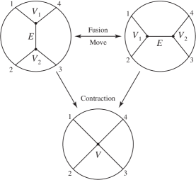
Figure 3.3. Fusion move and contraction.

Two $(d-3)$-dimensional cells are glued together along a $(d-4)$-dimensional cell. The number of $(d-3)$-dimensional cells in $X_{\succeq{\ast_{d}}}$ is equal to the Catalan number.

Theorem 3.3.

The space $X_{\succeq{\ast_{d}}}^{\rm{met}}$ is homeomorphic to $\mathbb{R}^{d-3}$, and its combinatorial structure defines a cell decomposition of $\mathbb{R}^{d-3}$, where each cell is a convex cone with vertex at the origin. The origin, corresponding to the graph ${\ast_{d}}$, is the only $0$-cell of the cell complex.

The group $\mathbb{Z}/d\mathbb{Z}$ acts on $X_{\succeq{\ast_{d}}}^{\rm{met}}$ through orthogonal transformations with respect to the natural Euclidean structure of $\mathbb{R}^{d-3}$.

Remark.

In [11], the rotation distance between the top dimensional cells of $X_{\succeq{\ast_{d}}}^{\rm{met}}$ was studied in terms of hyperbolic geometry, which has a connection to the structure of binary search trees.

Proof.

Draw a convex $d$-gon on the $xy$-plane in $xyz$-space. Let $\mathcal{V}$ be the set of vertices of the $d$-gon, and consider the set $f\in\mathbb{R}^{\mathcal{V}}$ of all functions

$$f:\mathcal{V}\longrightarrow\mathbb{R}.$$

An element $f\in\mathbb{R}^{\mathcal{V}}=\mathbb{R}^{d}$ can be represented by its function graph

(3.9) $$Graph(f)=\{(V,f(V))\;|\;V\in\mathcal{V}\}\subset\mathbb{R}^{3}.$$

Let us denote by $CH(Graph(f))$ the convex hull of $Graph(f)$ in $\mathbb{R}^{3}$. If we view the convex hull from the top, we see a $d$-gon with a set of non-intersecting diagonals.

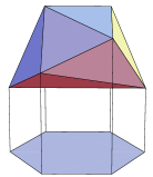
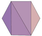
Figure 3.4. The convex hull of the function graph of $f\in\mathbb{R}^{\mathcal{V}}$ and its view from the top.

Viewing the convex hull from the positive direction of the $z$-axis, we obtain a map

(3.10) $$\xi:\mathbb{R}^{\mathcal{V}}\longrightarrow X_{\succeq{\ast_{d}}},$$

where we identify $X_{\succeq{\ast_{d}}}$ with the set of arrangements of non-intersecting diagonals of a convex $d$-gon. A generic point of $\mathbb{R}^{\mathcal{V}}$ corresponds to a triangulation of the $d$-gon as in Figure 3.4, but special points give fewer diagonals on the $d$-gon. For example, if $f$ is a constant function, then the function graph $Graph(f)$ is flat and the top view of its convex hull is just the $d$-gon without any diagonals in sight.

This consideration leads us to note that the map $\xi$ factors through

(3.11) $$\begin{CD}\mathbb{R}^{\mathcal{V}}@>{pr}>{}>\frac{\mathbb{R}^{\mathcal{V}}}{{\text{\rm{Affine}}}(\mathbb{R}^{2},\mathbb{R})}\\ \Big{\|}@V{}V{\eta}V\\ \mathbb{R}^{\mathcal{V}}@>{\xi}>{}>X_{\succeq{\ast_{d}}},\end{CD}$$

where

$${\text{\rm{Affine}}}(\mathbb{R}^{2},\mathbb{R})\cong\mathbb{R}^{3}$$

is the space of affine maps of $\mathbb{R}^{2}$ to $\mathbb{R}$. Such an affine map induces a map of $\mathcal{V}$ to $\mathbb{R}$, but the image is flat and no diagonals are produced in the $d$-gon.

The map $\eta$ of (3.11) is surjective, because we can explicitly construct a function $f$ that corresponds to an arbitrary element of $X_{\succeq{\ast_{d}}}$. We also note that the inverse image of an $m$-diagonal arrangement ($0\leq m\leq d-3$) is a cone of dimension $m$ with vertex at the origin. It is indeed a convex cone, because if two points of

(3.12) $$\frac{\mathbb{R}^{\mathcal{V}}}{{\text{\rm{Affine}}}(\mathbb{R}^{2},\mathbb{R})}=\mathbb{R}^{d-3}$$

correspond to the same diagonal arrangement of $X_{\succeq{\ast_{d}}}$, then every point on the line segment connecting these two points corresponds to the same arrangement. To see this, let $\mathcal{V}=\{V_{1},V_{2},\cdots,V_{d}\}$, and let a function $f\in\mathbb{R}^{\mathcal{V}}$ satisfy

$$f(V_{d-2})=f(V_{d-1})=f(V_{d})=0.$$

Then $f$ can be thought of an element of the quotient space (3.12). Take two such functions $f$ and $g$ that correspond to the same $m$-diagonal arrangement of the $d$-gon. The line segment connecting these two functions is

(3.13) $$h_{t}=f+t(g-f),$$

where $0\leq t\leq 1$. This means that the point $h_{t}(V_{j})\in\mathbb{R}^{3}$ is on the vertical line segment connecting $f(V_{j})$ and $g(V_{j})$ for all $j=1,2,3,\cdots,d-3.$ Thus the top roof of the convex hull $CH(Graph(h_{t}))$ determines the same arrangement of the diagonals on the $d$-gon as $CH(Graph(f))$ and $CH(Graph(g))$ do.

Since the inverse image of an $m$-diagonal arrangement is an $m$-dimensional convex cone, it is homeomorphic to $\mathbb{R}_{+}^{m}$. Hence $X_{\succeq{\ast_{d}}}$ defines a cell decomposition of $\mathbb{R}^{d-3}$, which is homeomorphic to $X_{\succeq{\ast_{d}}}^{\rm{met}}$, as claimed.

The convex $d$-gon on the plane can be taken as a regular $d$-gon centered at the origin. The cyclic group $\mathbb{Z}/d\mathbb{Z}$ naturally acts on $\mathcal{V}$ through rotations. This action induces an action on $\mathbb{R}^{\mathcal{V}}$ through permutation of axes, which is an orthogonal transformation with respect to the standard Euclidean structure of $\mathbb{R}^{d}$. A rotation of $\mathcal{V}$ induces a rotation of the horizontal plane $\mathbb{R}^{2}$, thus the space of affine maps of $\mathbb{R}^{2}$ to $\mathbb{R}$ is invariant under the $\mathbb{Z}/d\mathbb{Z}$-action. The action therefore descends to the orthogonal complement ${\text{\rm{Affine}}}(\mathbb{R}^{2},\mathbb{R})^{\perp}$ in $\mathbb{R}^{\mathcal{V}}$. Thus $\mathbb{Z}/d\mathbb{Z}$ acts on

$$X_{\succeq{\ast_{d}}}^{\rm{met}}\cong{\text{\rm{Affine}}}(\mathbb{R}^{2},\mathbb{R})^{\perp}\cong\mathbb{R}^{d-3}$$

by orthogonal transformations with respect to its natural Euclidean structure.

∎

Example 3.1.

The space of metric expansions of a vertex of degree $6$ is a cell decomposition of $\mathbb{R}^{3}$. There are nine $1$-cells, twenty-one $2$-cells, and fourteen $3$-cells. In Figure 3.5, the axes are depicted in the usual orientation, with the vertical axis representing the $z$ coordinate. The $\mathbb{Z}/6\mathbb{Z}$-action on $\mathbb{R}^{3}$ is generated by the orthogonal transformation

$$\begin{pmatrix}-\frac{1}{2}&0&\frac{\sqrt{3}}{2}\\ 0&-1&0\\ -\frac{\sqrt{3}}{2}&0&-\frac{1}{2}\end{pmatrix}.$$

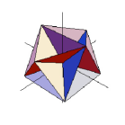
Figure 3.5. The space of metric expansions of a vertex of degree $6$.

Theorem 3.4.

Let $\Gamma\in RG_{g,n}$. Then

(3.14) $$X_{\succeq\Gamma}^{\rm{met}}\cong\mathbb{R}_{+}^{e(\Gamma)}\times\mathbb{R}^{6g-6+3n-e(\Gamma)}.$$

The combinatorial structure of $X_{\succeq\Gamma}$ determines a cell decomposition of $\mathbb{R}_{+}^{e(\Gamma)}\times\mathbb{R}^{6g-6+3n-e(\Gamma)}$. The group ${\text{\rm{Aut}}}(\Gamma)$ acts on $X_{\succeq\Gamma}^{\rm{met}}$ as automorphisms of the cell complex, which are orthogonal transformations with respect to its natural Euclidean structure through the homeomorphism (3.14). The action of ${\text{\rm{Aut}}}(\Gamma)$ on the metric edge space $\mathbb{R}_{+}^{e(\Gamma)}$ may be non-faithful (when $\Gamma$ is exceptional), but its action on $\mathbb{R}^{6g-6+3n-e(\Gamma)}$ is always faithful except for the case $(g,n)=(1,1)$.

Proof.

The expansion process of $\Gamma$ takes place at each vertex of degree $4$ or more. Since we identify expansions only when there is an isomorphism fixing all original half-edges coming from $\Gamma$, the expansion can be done independently at each vertex. Let $\ast(1),\cdots,\ast(v)$ be the list of vertices of $\Gamma$ and $d_{j}$ the degree of $\ast(j)$. We arrange the degree sequence of $\Gamma$ as

$$(\overset{n_{3}}{\overbrace{3,3,\cdots,3}},\overset{n_{4}}{\overbrace{4,4,\cdots,4}},\cdots,\overset{n_{m}}{\overbrace{m,m,\cdots,m}}).$$

Note that

$$n_{3}+n_{4}+\cdots+n_{m}=v=v(\Gamma)$$

is the number of vertices of $\Gamma$. Then

$$X_{\succeq\Gamma}^{\rm{met}}=\mathbb{R}_{+}^{e(\Gamma)}\times\prod_{j=1}^{v}X_{\succeq\ast(j)}^{\rm{met}},$$

and the second factor is homeomorphic to

$$\prod_{j=1}^{v}X_{\succeq\ast(j)}^{\rm{met}}\cong\prod_{\mu=3}^{m}\left(\mathbb{R}^{\mu-3}\right)^{n_{\mu}}=\mathbb{R}^{\rm{codim}(\Gamma)},$$

where

$${\rm{codim}}(\Gamma)=6g-6+3n-e(\Gamma)=\sum_{\mu=3}^{m}(\mu-3)n_{\mu}.$$

The group

$$G(\Gamma)=\prod_{\mu=3}^{m}\mathfrak{S}_{n_{\mu}}\rtimes\mathbb{Z}/\mu\mathbb{Z}$$

acts naturally on $\prod_{j=1}^{v}X_{\succeq\ast(j)}^{\rm{met}}$ through orthogonal transformations because each factor $\mathbb{Z}/\mu\mathbb{Z}$ acts on $X_{\succeq\ast(j)}^{\rm{met}}$ through orthogonal transformations if $d_{j}=\mu$, and the symmetric group $\mathfrak{S}_{n_{\mu}}$ acts on $\left(\mathbb{R}^{\mu-3}\right)^{n_{\mu}}$ by permutations of factors, which are also orthogonal transformations.

Since ${\text{\rm{Aut}}}(\Gamma)$ is a subgroup of $G(\Gamma)$, it acts on $\prod_{j=1}^{v}X_{\succeq\ast(j)}^{\rm{met}}$ through orthogonal transformations. It’s action on $\mathbb{R}_{+}^{e(\Gamma)}$ is by permutations of axes, thus it is also orthogonal in the standard embedding of $\mathbb{R}_{+}^{e(\Gamma)}$ into $\mathbb{R}^{e(\Gamma)}$. Therefore, ${\text{\rm{Aut}}}(\Gamma)$ acts on $X_{\succeq\Gamma}^{\rm{met}}$ through orthogonal transformations with respect to the natural Euclidean structure of $X_{\succeq\Gamma}^{\rm{met}}$.

The action of ${\text{\rm{Aut}}}(\Gamma)$ on $\mathbb{R}^{\rm{codim}(\Gamma)}$ is faithful because all half-edges of $\Gamma$ are labeled in $X_{\succeq\Gamma}^{\rm{met}}$, except for the case $(g,n)=(1,1)$. There are only two graphs in $RG_{1,1}$, and both are exceptional. Thus the ${\text{\rm{Aut}}}(\Gamma)$-action on $X_{\succeq\Gamma}^{\rm{met}}$ has a redundant factor $\mathbb{Z}/2\mathbb{Z}$ for $RG_{1,1}$. ∎

Theorem 3.5.

The space

$$RG_{g,n}^{\rm{met}}=\coprod_{\Gamma\in RG_{g,n}}\frac{\mathbb{R}_{+}^{e(\Gamma)}}{{\text{\rm{Aut}}}(\Gamma)}$$

of metric ribbon graphs is a differentiable orbifold locally modeled by

(3.15) $$\frac{X_{\succeq\Gamma}^{\rm{met}}}{{\text{\rm{Aut}}}(\Gamma)}.$$

Proof.

For every ribbon graph ${\Gamma}\in RG_{g,n}$, there is a natural map

(3.16) $$\widetilde{\mu}_{\Gamma}:X_{\succeq\Gamma}^{\rm{met}}\longrightarrow RG_{g,n}^{\rm{met}},$$

assigning to each metric expansion of $\Gamma$ its isomorphism class as a metric ribbon graph. Since the ${\text{\rm{Aut}}}(\Gamma)$-action on $X_{\succeq\Gamma}^{\rm{met}}$ induces ribbon graph isomorphisms, the map (3.16) factors through the map $\mu_{\Gamma}$ of the quotient space:

(3.17) $$X_{\succeq\Gamma}^{\rm{met}}\longrightarrow\frac{X_{\succeq\Gamma}^{\rm{met}}}{{\text{\rm{Aut}}}(\Gamma)}\overset{\mu_{\Gamma}}{\longrightarrow}RG_{g,n}^{\rm{met}}.$$

The inverse image $\widetilde{\mu}_{\Gamma}^{-1}(U_{\epsilon}(\Gamma_{\rm{met}}))$ of the $\epsilon$-neighborhood $U_{\epsilon}(\Gamma_{\rm{met}})$ is an open subset of $X_{\succeq\Gamma}^{\rm{met}}$ that is homeomorphic to a disk. We claim that

(3.18) $$\mu_{\Gamma}:\frac{\widetilde{\mu}_{\Gamma}^{-1}(U_{\epsilon}(\Gamma_{\rm{met}}))}{{\text{\rm{Aut}}}(\Gamma)}\overset{\sim}{\longrightarrow}U_{\epsilon}(\Gamma_{\rm{met}})$$

is a homeomorphism for every metric ribbon graph $\Gamma_{\rm{met}}$ if $\epsilon>0$ is chosen sufficiently small compared to the shortest edge length of $\Gamma_{\rm{met}}$.

Take a point $\Gamma_{\rm{met}}^{0}\in U_{\epsilon}(\Gamma_{\rm{met}})$, and let

$$\Gamma_{\rm{met}}^{j}\in\widetilde{\mu}_{\Gamma}^{-1}(\Gamma_{\rm{met}}^{0}),\qquad j=1,2,$$

be two inverse images. The ribbon graph isomorphism $\widetilde{\alpha}$ that brings $\Gamma_{\rm{met}}^{1}$ to $\Gamma_{\rm{met}}^{2}$ preserves the set $K$ of contracting edges. Since $\Gamma_{\rm{met}}^{j}$ modulo the contracting edges $K$ is the graph $\Gamma_{\rm{met}}$, $\widetilde{\alpha}$ induces an automorphism $\alpha\in{\text{\rm{Aut}}}(\Gamma)$. Thus $\widetilde{\alpha}$ factors into the product of an automorphism $\alpha$ of $\Gamma$ and a permutation of $K$. As an element of $X_{\succeq\Gamma}^{\rm{met}}$, a permutation of contracting edges in $K$ fixes the element. Thus $\Gamma_{\rm{met}}^{2}$ is an $\alpha$-image of $\Gamma_{\rm{met}}^{1}$ in $X_{\succeq\Gamma}^{\rm{met}}$. This shows that (3.18) is a natural bijection.

Since the topology of the space of metric ribbon graphs is determined by these $\epsilon$-neighborhoods, the map $\mu_{\Gamma}$ is continuous. Thus for a small enough $\epsilon$, we have a homeomorphism (3.18).

The metric ribbon graph space is covered by local coordinate patches

(3.19) $$\bigcup_{\Gamma\in RG_{g,n}^{\rm{met}}}\mu_{\Gamma}\left(\frac{\widetilde{\mu}_{\Gamma}^{-1}(U_{\epsilon}(\Gamma_{\rm{met}}))}{{\text{\rm{Aut}}}(\Gamma)}\right)=RG_{g,n}^{\rm{met}},$$

where

$$\frac{\widetilde{\mu}_{\Gamma}^{-1}(U_{\epsilon}(\Gamma_{\rm{met}}))}{{\text{\rm{Aut}}}(\Gamma)}\subset\frac{X_{\succeq\Gamma}^{\rm{met}}}{{\text{\rm{Aut}}}(\Gamma)}$$

is a differentiable orbifold. Let

$$\Gamma_{\rm{met}}^{\prime\prime}\in\mu_{\Gamma}\left(\frac{\widetilde{\mu}_{\Gamma}^{-1}(U_{\epsilon}(\Gamma_{\rm{met}}))}{{\text{\rm{Aut}}}(\Gamma)}\right)\cap\mu_{\Gamma^{\prime}}\left(\frac{\widetilde{\mu}_{\Gamma^{\prime}}^{-1}(U_{\epsilon}(\Gamma_{\rm{met}}^{\prime}))}{{\text{\rm{Aut}}}(\Gamma^{\prime})}\right)$$

be a metric ribbon graph in the intersection of two coordinate patches. Then $\Gamma^{\prime\prime}\succeq\Gamma$ and $\Gamma^{\prime\prime}\succeq\Gamma^{\prime}$. There is a small $\delta$ such that

$$\mu_{\Gamma^{\prime\prime}}\left(\frac{\widetilde{\mu}_{\Gamma^{\prime\prime}}^{-1}(U_{\delta}(\Gamma_{\rm{met}}^{\prime\prime}))}{{\text{\rm{Aut}}}(\Gamma^{\prime\prime})}\right)\subset\mu_{\Gamma}\left(\frac{\widetilde{\mu}_{\Gamma}^{-1}(U_{\epsilon}(\Gamma_{\rm{met}}))}{{\text{\rm{Aut}}}(\Gamma)}\right)\cap\mu_{\Gamma^{\prime}}\left(\frac{\widetilde{\mu}_{\Gamma^{\prime}}^{-1}(U_{\epsilon}(\Gamma_{\rm{met}}^{\prime}))}{{\text{\rm{Aut}}}(\Gamma^{\prime})}\right).$$

If we label the edges of $\Gamma^{\prime\prime}$ that are not contracted in $\Gamma$, then we have an embedding

$$X_{\succeq\Gamma^{\prime\prime}}^{\rm{met}}\subset X_{\succeq\Gamma}^{\rm{met}}$$

that induces

$$\frac{\widetilde{\mu}_{\Gamma^{\prime\prime}}^{-1}(U_{\delta}(\Gamma_{\rm{met}}^{\prime\prime}))}{{\text{\rm{Aut}}}(\Gamma^{\prime\prime})}\subset\frac{\widetilde{\mu}_{\Gamma}^{-1}(U_{\epsilon}(\Gamma_{\rm{met}}))}{{\text{\rm{Aut}}}(\Gamma)}.$$

These inclusion maps are injective diffeomorphisms with respect to the natural differentiable structure of $X_{\succeq\Gamma}^{\rm{met}}$. The same is true for $\Gamma^{\prime\prime}$ and $\Gamma^{\prime}$. This implies that the local coordinate neighborhoods of (3.19) are patched together by diffeomorphisms. ∎

Remark.

The local map $\mu_{\Gamma}$ of (3.18) is not a homeomorphism if $\epsilon$ takes a large value. In particular,

$$\frac{X_{\succeq\Gamma}^{\rm{met}}}{{\text{\rm{Aut}}}(\Gamma)}$$

does not map injectively to $RG_{g,n}^{\rm{met}}$ via the natural map $\mu_{\Gamma}$.

Theorem 3.6.

The Euler characteristic of $RG_{g,n}^{\rm{met}}$ as an orbifold is given by

(3.20) $${\hbox{\raise 1.5pt\hbox{$\chi$}}}(RG_{g,n}^{\rm{met}})=\sum_{\Gamma\in RG_{g,n}}\frac{(-1)^{e(\Gamma)}}{|{\text{\rm{Aut}}}(\Gamma)|},\qquad(g,n)\neq(1,1).$$

For $(g,n)=(1,1)$, we have

(3.21) $${\hbox{\raise 1.5pt\hbox{$\chi$}}}(RG_{1,1}^{\rm{met}})=\sum_{\Gamma\in RG_{1,1}}\frac{(-1)^{e(\Gamma)}}{|{\text{\rm{Aut}}}(\Gamma)|/2}=-\frac{1}{3}+\frac{1}{2}=\frac{1}{6}.$$

Proof.

Since the ${\text{\rm{Aut}}}(\Gamma)$-action on $\mathbb{R}_{+}^{e(\Gamma)}$ is through the representation

$${\text{\rm{Aut}}}(\Gamma)\longrightarrow\mathfrak{S}_{e(\Gamma)},$$

we have the canonical orbifold cell decomposition of $\mathbb{R}_{+}^{e(\Gamma)}/{\text{\rm{Aut}}}(\Gamma)$ defined in Example 2.1. Gluing all these canonical cell decompositions of the rational cells of the orbifold $RG_{g,n}^{\rm{met}}$, we obtain an orbifold cell decomposition of the entire space $RG_{g,n}^{\rm{met}}$. To determine the isotropy subgroups of each orbifold cell, we need the local model (3.18). We note that the ${\text{\rm{Aut}}}(\Gamma)$-action on $\widetilde{\mu}_{\Gamma}^{-1}(U_{\epsilon}(\Gamma_{\rm{met}}))$ is faithful if $(g,n)\neq(1,1)$. If ${\text{\rm{Aut}}}(\Gamma)$ acts on $\mathbb{R}_{+}^{e(\Gamma)}$ faithfully, then the contribution of the rational cell $\mathbb{R}_{+}^{e(\Gamma)}/{\text{\rm{Aut}}}(\Gamma)$ to the Euler characteristic of $RG_{g,n}^{\rm{met}}$ is

$$\frac{(-1)^{e(\Gamma)}}{|{\text{\rm{Aut}}}(\Gamma)|}.$$

But if $\Gamma$ is exceptional, then the rational cell

$$\frac{\mathbb{R}_{+}^{e(\Gamma)}}{{\text{\rm{Aut}}}(\Gamma)}=\frac{\mathbb{R}_{+}^{e(\Gamma)}}{{\text{\rm{Aut}}}(\Gamma)/(\mathbb{Z}/2\mathbb{Z})}$$

is itself a singular set of $X_{\succeq\Gamma}^{\rm{met}}/{\text{\rm{Aut}}}(\Gamma)$. The contribution of the Euler characteristic of $RG_{g,n}^{\rm{met}}$ from this rational cell is thus

$$\frac{(-1)^{e(\Gamma)}}{2\cdot|{\text{\rm{Aut}}}(\Gamma)/(\mathbb{Z}/2\mathbb{Z})|}=\frac{(-1)^{e(\Gamma)}}{|{\text{\rm{Aut}}}(\Gamma)|}.$$

Summing all these, we obtain the formula for the Euler characteristic.

The case of $(g,n)=(1,1)$ is still different because all graphs in $RG_{1,1}$ are exceptional. The general formula (3.20) gives $-1/6+1/4=1/12$, but since the factor $\mathbb{Z}/2\mathbb{Z}$ of ${\text{\rm{Aut}}}(\Gamma)$ acts trivially on $X_{\succeq\Gamma}^{\rm{met}}$, the factor $2$ has to be modified. ∎

The computation of (3.20) was first done in [4] using a combinatorial argument, and then in [7] and [6] using an asymptotic analysis of Hermitian matrix integrals. The result is

(3.22) $$\sum_{\Gamma\in RG_{g,n}}\frac{(-1)^{e(\Gamma)}}{|{\text{\rm{Aut}}}(\Gamma)|}=-\frac{(2g+n-3)!(2g)(2g-1)}{(2g)!n!}\zeta(1-2g)$$

for every $g\geq 0$ and $n>0$ subject to $2-2g-n<0$.

Let $RGB_{g,n}$ denote the set of isomorphism classes of connected ribbon graphs with labeled boundary components subject to the topological condition (3.1), and

(3.23) $$RGB_{g,n}^{\text{met}}=\coprod_{\Gamma\in RGB_{g,n}}\frac{\mathbb{R}_{+}^{e(\Gamma)}}{{\text{\rm{Aut}}}_{\partial}(\Gamma)}$$

the space of metric ribbon graphs with labeled boundary components, where

$${\text{\rm{Aut}}}_{\partial}(\Gamma)$$

is the automorphism group of a ribbon graph $\Gamma$ preserving the boundary labeling. The same argument of the previous section applies without any alteration to show that $RGB_{g,n}^{\text{met}}$ is a differentiable orbifold locally modeled by

$$\frac{X_{\succeq\Gamma}^{\rm{met}}}{{\text{\rm{Aut}}}_{\partial}(\Gamma)}.$$

The definition of the space of metric expansions $X_{\succeq\Gamma}^{\rm{met}}$ does not refer to the labeling of the boundary components of a ribbon graph $\Gamma$, but it requires labeling of all half-edges of $\Gamma$. As we noted at the end of Section 1, labeling of the half-edges induces an order of boundary components. Thus every expansion of $\Gamma$ appearing in $X_{\succeq\Gamma}^{\rm{met}}$ has a boundary labeling that is consistent with the boundary labeling of $\Gamma$.

Theorem 3.7.

For every genus $g\geq 0$ and $n\geq 1$ subject to (3.6), the natural forgetful projection

(3.24) $$pr:RGB_{g,n}^{\text{met}}\longrightarrow RG_{g,n}^{\text{met}}$$

is an orbifold covering of degree $n!$.

Proof.

Let $\Gamma$ be a ribbon graph. We label the boundary components of $\Gamma$, and denote by $B$ the set of all permutations of the boundary components. The cardinality $|B|$ of $B$ is $n!$. The automorphism group ${\text{\rm{Aut}}}(\Gamma)$ acts on the set $B$, and by definition the isotropy subgroup of ${\text{\rm{Aut}}}(\Gamma)$ of each element of $B$ is isomorphic to the group ${\text{\rm{Aut}}}_{\partial}(\Gamma)$. The orbit space $B/{\text{\rm{Aut}}}(\Gamma)$ is the set of ribbon graphs with labeled boundary. Thus the inverse image of the local model $X_{\succeq\Gamma}^{\rm{met}}/{\text{\rm{Aut}}}(\Gamma)$ by $pr^{-1}$ is the disjoint union of $|B/{\text{\rm{Aut}}}(\Gamma)|$ copies of $X_{\succeq\Gamma}^{\rm{met}}/{\text{\rm{Aut}}}_{\partial}(\Gamma)$:

(3.25) $$pr^{-1}\left(\frac{X_{\succeq\Gamma}^{\rm{met}}}{{\text{\rm{Aut}}}(\Gamma)}\right)=\overset{|B/{\text{\rm{Aut}}}(\Gamma)|{\text{-copies}}}{\overbrace{\frac{X_{\succeq\Gamma}^{\rm{met}}}{{\text{\rm{Aut}}}_{\partial}(\Gamma)}\coprod\cdots\coprod\frac{X_{\succeq\Gamma}^{\rm{met}}}{{\text{\rm{Aut}}}_{\partial}(\Gamma)}}}.$$

Since the projection restricted to each local model

$$pr:\frac{X_{\succeq\Gamma}^{\rm{met}}}{{\text{\rm{Aut}}}_{\partial}(\Gamma)}\longrightarrow\frac{X_{\succeq\Gamma}^{\rm{met}}}{{\text{\rm{Aut}}}(\Gamma)}$$

is an orbifold covering of degree $|{\text{\rm{Aut}}}(\Gamma)/{\text{\rm{Aut}}}_{\partial}(\Gamma)|$, the map

(3.26) $$pr_{\Gamma}:pr^{-1}\left(\frac{X_{\succeq\Gamma}^{\rm{met}}}{{\text{\rm{Aut}}}(\Gamma)}\right)\longrightarrow\frac{X_{\succeq\Gamma}^{\rm{met}}}{{\text{\rm{Aut}}}(\Gamma)}$$

is an orbifold covering of degree

$$|B/{\text{\rm{Aut}}}(\Gamma)|\cdot|{\text{\rm{Aut}}}(\Gamma)/{\text{\rm{Aut}}}_{\partial}(\Gamma)|=|B|=n!.$$

Since the projection of (3.24) is just a collection of $pr_{\Gamma}$ of (3.26),

$$pr:RGB_{g,n}^{\rm{met}}\longrightarrow{RG}_{g,n}^{\rm{met}}$$

is an orbifold covering of degree $n!$ as desired. ∎

As an immediate consequence, we have

Corollary 3.8.

The Euler characteristic of $RGB_{g,n}^{\rm{met}}$ is given by

(3.27) $${\hbox{\raise 1.5pt\hbox{$\chi$}}}(RGB_{g,n}^{\rm{met}})=n!\cdot{\hbox{\raise 1.5pt\hbox{$\chi$}}}(RG_{g,n}^{\rm{met}}).$$

4. Strebel differentials on Riemann surfaces

A Riemann surface is a patchwork of complex domains. Let us ask the question in the opposite direction: If we are given a compact Riemann surface, then how can we find coordinate patches that represent the complex structure? In this section we give a canonical coordinate system on a Riemann surface once a finite number of points on the surface and the same number of positive real numbers are chosen. The key technique is the theory of Strebel differentials [12]. Using Strebel differentials, we can encode the holomorphic structure of a Riemann surface in the combinatorial data of ribbon graphs.

Let $C$ be a compact Riemann surface. We choose a finite set of labeled points $\{p_{1},p_{2},\cdots,p_{n}\}$ on $C$, and call them marked points on the Riemann surface. The bridge that connects the complex structure of a Riemann surface and combinatorial data is the Strebel differential on the Riemann surface. Let $K_{C}$ be the canonical sheaf of $C$. A holomorphic quadratic differential defined on $C$ is an element of $H^{0}(C,K_{C}^{\otimes 2})$, where $K_{C}^{\otimes 2}$ denotes the symmetric tensor product of the canonical sheaf. In a local coordinate $z$ on $C$, a quadratic differential $q$ is represented by $q=f(z)\big{(}dz\big{)}^{2}$ with a locally defined holomorphic function $f(z)$. With respect to a coordinate change $w=w(z)$, the local expressions

$$q=f(z)\big{(}dz\big{)}^{2}=g(w)\big{(}dw\big{)}^{2}$$

transform by

(4.1) $$f(z)=g(w(z))\left(\frac{dw(z)}{dz}\right)^{2}.$$

A meromorphic quadratic differential on $C$ is a holomorphic quadratic differential $q$ defined on $C$ except for a finite set $\{p_{1},\cdots,p_{n}\}$ of points of $C$ such that at each singularity $p_{j}$ of $q$, there is a local expression $q=f_{j}(z)\big{(}dz\big{)}^{2}$ with a meromorphic function $f_{j}$ that has a pole at $z=p_{j}$. If $f_{j}(z)$ has a pole of order $r$ at $p_{j}$, then we say $q$ has a pole of order $r$ at $z=p_{j}$.

Let $q=f(z)\big{(}dz\big{)}^{2}$ be a meromorphic quadratic differential defined on $C$. A real parametric curve

(4.2) $$\gamma:(a,b)\owns t\longmapsto\gamma(t)=z\in C$$

parameterized on an open interval $(a,b)$ of a real axis is a horizontal leaf (or in the classical terminology, a horizontal trajectory) of $q$ if

(4.3) $$f(\gamma(t))\left(\frac{d\gamma(t)}{dt}\right)^{2}>0$$

for every $t\in(a,b)$. If

(4.4) $$f(\gamma(t))\left(\frac{d\gamma(t)}{dt}\right)^{2}<0$$

holds instead, then the parametric curve $\gamma$ of (4.2) is called a vertical leaf of $q$. The collection of all horizontal or vertical leaves form a real codimension 1 foliation on the Riemann surface $C$ minus the singular points and zeroes of $q$. There are three important examples of the foliations for our study.

Example 4.1.

Let $q=\big{(}dz\big{)}^{2}$. Then the horizontal lines

$$\alpha(t)=t+ci,\qquad t\in{\mathbb{R}}$$

are the horizontal leaves of $q$, and

$$\beta(t)=it+c,\qquad t\in{\mathbb{R}}$$

are the vertical leaves for every $c\in{\mathbb{R}}$. Each of these defines a simple foliation on the complex plane $\mathbb{C}$. In Figure 4.1, horizontal leaves are described by straight lines, and vertical leaves are indicated by broken lines.

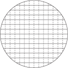
Figure 4.1. Foliations defined by $(dz)^{2}$.

If a quadratic differential $q=f(z)(dz)^{2}$ is holomorphic and non-zero at $z=z_{0}$, then on a neighborhood of $z_{0}$ we can introduce a canonical coordinate

(4.5) $$w(z)=\int_{z_{0}}^{z}\sqrt{f(z)}dz.$$

It follows from (4.1) that in the $w$-coordinate the quadratic differential is given by $q=(dw)^{2}$. Therefore, the leaves of $q$ near $z_{0}$ look exactly as in Figure 4.1 in the canonical coordinate. This explains the classical terminology of horizontal and vertical trajectories. We remark here that although the coordinate $w(z)$ is called canonical, still there is an ambiguity of coordinate change

(4.6) $$w(z)\longmapsto-w(z)+a$$

with an arbitrary complex constant $a$.

Using the canonical coordinate, it is obvious to see the following:

Proposition 4.1.

Let $S$ be an open Riemann surface and $q$ a holomorphic quadratic differential on $S$. Then for every point $p\in S$, there is a unique horizontal leaf and a vertical leaf passing through $p$. Moreover, these leaves intersect at a right angle with respect to the conformal structure of $S$ near $p$.

When a holomorphic quadratic differential has a zero, then the foliation behaves differently.

Example 4.2.

Let $q=z^{m}(dz)^{2}$. Then $(m+2)$ half rays

$$\alpha_{k}:(0,\infty)\owns t\longmapsto t\cdot{\text{\rm{exp}}}\left(\frac{2\pi ik}{m+2}\right)\in\mathbb{C},\qquad k=0,1,\cdots,m+1$$

give the horizontal leaves that have $z=0$ on the boundary (the straight lines of Figure 4.2), and another set of $(m+2)$ half rays

$$\beta_{k}:(0,\infty)\owns t\longmapsto t\cdot{\text{\rm{exp}}}\left(\frac{\pi i+2\pi ik}{m+2}\right)\in\mathbb{C},\qquad k=0,1,\cdots,m+1$$

gives the vertical leaves (the broken lines of Figure 4.2).

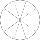
Figure 4.2. Horizontal and vertical leaves of $z^{3}(dz)^{2}$.

The foliation becomes quite wild at singularities of $q$. However, the situation is milder around a quadratic pole with a negative real coefficient .

Example 4.3.

Let $q=-\left(\frac{dz}{z}\right)^{2}$. Then every concentric circle centered at $0$,

$$\alpha(t)=re^{it},\qquad t\in\mathbb{R},r>0,$$

is a horizontal leaf, and all the half-rays

$$\beta(t)=te^{i\theta},\qquad t>0,0\leq\theta<2\pi,$$

give the vertical leaves. We note that all horizontal leaves are compact curves (Figure 4.3).

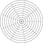
Figure 4.3. Horizontal compact leaves and vertical leaves of $-\frac{1}{z^{2}}(dz)^{2}$.

The fundamental theorem we need is:

Theorem 4.2 (Strebel [12]).

Let $g$ and $n$ be integers satisfying that

(4.7) $$\begin{cases}g\geq 0\\ n\geq 1\\ 2-2g-n<0,\end{cases}$$

and $(C,(p_{1},\cdots,p_{n}))$ a smooth Riemann surface of genus $g$ with $n$ marked points $p_{1},\cdots,p_{n}$. Choose an ordered $n$-tuple $(a_{1},\cdots,a_{n})\in\mathbb{R}_{+}^{n}$ of positive real numbers. Then there is a unique meromorphic quadratic differential $q$ on $C$ satisfying the following conditions:

1. $q$ is holomorphic on $C\setminus\{p_{1},\cdots,p_{n}\}$.

2. $q$ has a double pole at each $p_{j}$, $j=1,\cdots,n$.

3. The union of all noncompact horizontal leaves forms a closed subset of $C$ of measure zero.

4. Every compact horizontal leaf $\alpha$ is a simple loop circling around one of the poles, say $p_{j}$, and it satisfies

   (4.8) $$a_{j}=\oint_{\alpha}\sqrt{q},$$

   where the branch of the square root is chosen so that the integral has a positive value with respect to the positive orientation of $\alpha$ that is determined by the complex structure of $C$.

This unique quadratic differential is called the Strebel differential. Note that the integral (4.8) is automatically a real number because of (4.3). Every noncompact horizontal leaf of a Strebel differential defined on $C$ is bounded by zeros of $q$, and every zero of degree $m$ of $q$ bounds $m+2$ horizontal leaves, as we have seen in Example 4.2.

Let $\gamma(t)$ be a noncompact horizontal leaf bounded by two zeros $z_{0}=\gamma(t_{0})$ and $z_{1}=\gamma(t_{1})$ of $q=f(z)(dz)^{2}$. Then we can assign a positive real number

(4.9) $$L(\gamma)=\int_{z_{0}}^{z_{1}}\sqrt{q}=\int_{t_{0}}^{t_{1}}\sqrt{f(\gamma(t))}\frac{d\gamma(t)}{dt}dt$$

by choosing a branch of $\sqrt{f(z)}$ near $z_{0}$ and $z_{1}$ so that the integral becomes positive. As before, the integral is a real number because $\gamma$ is a horizontal leaf. We call $L(\gamma)$ the length of the edge $\gamma$ with respect to $q$. Note that the length (4.9) is independent of the choice of the parameter $t$. The length is also defined for any compact horizontal leaf by (4.8). Thus every horizontal leaf has a uniquely defined length, and hence the Strebel differential $q$ defines a measured foliation on the open subset of the Riemann surface that is the complement of the set of zeroes and poles of $q$.

Around every marked point $p_{j}$ there is a foliated disk of compact horizontal leaves with length equal to the prescribed value $a_{j}$. As the loop becomes larger in size (but not in length, because it is a constant), it hits zeroes of $q$ and the shape becomes a polygon (Figure 4.4).

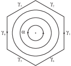
Figure 4.4. A foliated disk with compact horizontal leaves.

Let the polygon be an $m$-gon, $\gamma_{1},\cdots,\gamma_{m}$ the noncompact horizontal leaves surrounding $p_{j}$, and $\alpha$ a compact horizontal leaf around the point. Then we have

(4.10) $$a_{j}=L(\alpha)=L(\gamma_{1})+\cdots L(\gamma_{m}).$$

We note that some of the $\gamma_{j}$’s may be the same noncompact horizontal leaf on the Riemann surface $C$. The collection of all compact horizontal leaves surrounding $p_{j}$ forms a punctured disk with its center at $p_{j}$. Glue all these punctured disks to noncompact horizontal leaves and the zeroes of the Strebel differentials, and fill the punctures with points $\{p_{1},\cdots,p_{n}\}$. Then we obtain a compact surface, which is the underlying topological surface of the Riemann surface $C$.

Corollary 4.3.

Let $g$ and $n$ be integers satisfying (4.7), and

(4.11) $$(C,(p_{1},p_{2},\cdots,p_{n}),(a_{1},a_{2},\cdots,a_{n}))$$

a nonsingular Riemann surface of genus $g$ with $n$ marked points and an ordered $n$-tuple of positive real numbers. Then there is a unique cell-decomposition $\square_{q}$ of $C$ consisting of $v$ $0$-cells, $e$ $1$-cells, and $n$ $2$-cells, where $v$ is the number of zeroes of the Strebel differential $q$ associated with (4.11), and

$$e=v-2+2g+n.$$

Proof.

The $0$-cells, or the vertices, of $\square_{q}$ are the zeroes of the Strebel differential $q$ of (4.11). The $1$-cells, or the edges, are the noncompact horizontal leaves that connect the $0$-cells. Since each $1$-cell has a finite positive length and the union of all $1$-cells is closed and has measure zero on $C$, the number of $1$-cells is finite. The union of all compact horizontal leaves that are homotopic to $p_{j}$ (together with the center $p_{j}$) forms a $2$-cell, or a face, that is homeomorphic to a $2$-disk. There are $n$ such $2$-cells. The formula for the Euler characteristic

$$v-e+n=2-2g$$

determines the number of edges. ∎

The $1$-skeleton, or the union of the $0$-cells and $1$-cells, of the cell-decomposition $\square_{q}$ that is defined by the Strebel differential is a ribbon graph. The cyclic order of half-edges at each vertex is determined by the orientation of the Riemann surface. A vertex of the graph that comes from a zero of degree $m$ of the Strebel differential has degree $m+2$. Thus the graph we are considering here does not have any vertices of degree less than $3$. Since each edge of the graph has the unique length by (4.9), the graph is a metric ribbon graph.

Let us give some explicit examples of the Strebel differentials. We start with a meromorphic quadratic differential which is not a Strebel differential, but nonetheless an important example because it plays the role of a building block.

Example 4.4.

Consider the meromorphic quadratic differential

(4.12) $$q_{0}=\frac{1}{4\pi^{2}}\frac{(d\zeta)^{2}}{\zeta(1-\zeta)}=\frac{1}{4\pi^{2}}\left(\frac{1}{\zeta}+\frac{1}{1-\zeta}\right)(d\zeta)^{2}$$

on $\mathbb{P}^{1}$. It has simple poles at $0$ and $1$, and a double pole at $\infty$. The line segment $[0,1]$ is a horizontal leaf of length $1/2$. The whole $\mathbb{P}^{1}$ minus $[0,1]$ and infinity is covered with a collection of compact horizontal leaves which are confocal ellipses

(4.13) $$\zeta=a\cos\theta+\frac{1}{2}+ib\sin\theta,$$

where $a$ and $b$ are positive constants that satisfy

$$a^{2}=b^{2}+\frac{1}{4}.$$

We have

$$\frac{1}{4\pi^{2}}\frac{(d\zeta)^{2}}{\zeta(1-\zeta)}=\frac{1}{4\pi^{2}}(d\theta)^{2}$$

under (4.13). The length of each compact leaf is $1$.

Figure 4.5. Horizontal leaves of $\frac{1}{4\pi^{2}}\frac{(d\zeta)^{2}}{\zeta(1-\zeta)}$.

Example 4.5.

Recall the Weierstrass elliptic function

(4.14) $$\begin{split}\wp(z)&=\frac{1}{z^{2}}+\sum_{\begin{subarray}{c}(m,n)\in\mathbb{Z}^{2}\\ (m,n)\neq(0,0)\end{subarray}}\left(\frac{1}{(z-m-n\tau)^{2}}-\frac{1}{(m+n\tau)^{2}}\right)\\ &=\frac{1}{z^{2}}+\frac{g_{2}z^{2}}{20}+\frac{g_{3}z^{4}}{28}+\frac{g_{2}^{2}z^{6}}{1200}+\frac{3g_{2}g_{3}z^{8}}{6160}+\cdots\end{split}$$

defined on the elliptic curve

(4.15) $$E_{\tau}=\frac{\mathbb{C}}{\mathbb{Z}\oplus\mathbb{Z}\tau}$$

of modulus $\tau$ with $Im(\tau)>1$, where $g_{2}$ and $g_{3}$ are defined by

(4.16) $$g_{2}=\sum_{\begin{subarray}{c}(m,n)\in\mathbb{Z}^{2}\\ (m,n)\neq(0,0)\end{subarray}}\frac{60}{(m+n\tau)^{4}},\quad\text{and}\quad g_{3}=\sum_{\begin{subarray}{c}(m,n)\in\mathbb{Z}^{2}\\ (m,n)\neq(0,0)\end{subarray}}\frac{140}{(m+n\tau)^{6}}.$$

Let $z$ be a coordinate on $E_{\tau}$. It is customary to write

$$\omega_{1}=1/2,\quad\omega_{2}=(1+\tau)/2,\quad\quad\omega_{3}=\tau/2$$

and

$$e_{j}=\wp(\omega_{j}),\qquad j=1,2,3.$$

The quantities $g_{2}$, $g_{3}$ and $e_{j}$’s satisfy the following relation:

$$4x^{3}-g_{2}x-g_{3}=4(x-e_{1})(x-e_{2})(x-e_{3}).$$

Let us consider the case when $\tau=i=\sqrt{-1}$. We have $g_{2}=4$, $g_{3}=0$, $e_{1}=-e_{3}=1$ and $e_{2}=0$. In particular, the elliptic curve is defined over $\mathbb{Q}$. The Weierstrass $\wp$-function maps the interior of the square spanned by $0,\omega_{1},\omega_{2},\omega_{3}$ biholomorphically onto the upper half plane, and the boundary of the square to the real axis (see for example, [8]). A Strebel differential is given by

(4.17) $$q=-\frac{4}{\pi^{2}}\wp(z)(dz)^{2}.$$

The series expansion of (4.14) tells us that the horizontal leaves near $0$ are closed loops that are centered at the origin. The differential $q$ has a double zero at $\omega_{2}$, which we see from the Weierstrass differential equation

$$\wp^{\prime}(z)^{2}=4\wp(z)^{3}-4\wp(z)=4\left(\wp(z)-e_{1}\right)\left(\wp(z)-e_{2}\right)\left(\wp(z)-e_{3}\right).$$

The real curve $\omega_{1}+it$ is a horizontal leaf, because on the edge $\overline{\omega_{1}\omega_{2}}$ the Weierstrass function $\wp(z)$ takes values in $[e_{2},e_{1}]$. The curve $\omega_{3}+t$ is also a horizontal leaf, because on the edge $\overline{\omega_{3}\omega_{2}}$ the function $\wp(z)$ takes values in $[e_{3},e_{2}]$. In the above consideration we used the fact that $\wp(z)$ is an even function:

$$\wp(z)=\wp(-z).$$

An extra $\mathbb{Z}/2\mathbb{Z}$ symmetry comes from the transformation property

$$\wp(iz)=-\wp(z).$$

To prove that (4.17) is indeed a Strebel differential, we just note that $q$ is the pull-back of the building block $q_{0}$ of (4.12) via a holomorphic map

(4.18) $$\phi:E_{i}\overset{\wp^{2}}{\longrightarrow}\mathbb{P}^{1}.$$

Indeed,

$$q=-\frac{4}{\pi^{2}}\wp(z)(dz)^{2}=\frac{1}{4\pi^{2}}\frac{(d\wp^{2})^{2}}{\wp^{2}(1-\wp^{2})}.$$

The inverse image of the interval $[0,1]$ is the degree $4$ ribbon graph with one vertex, two edges and one boundary component (Figure 4.6).

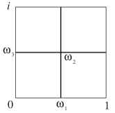
Figure 4.6. Elliptic curve of modulus $\tau=i$ and a ribbon graph on it.

Another interesting case is $\tau=e^{\pi i/3}$, which corresponds to $g_{2}=0$, $g_{3}=4$, and

$$e_{1}=1,\quad e_{2}=e^{2\pi i/3},\quad e_{3}=e^{4\pi i/3}.$$

Again the elliptic curve is defined over $\mathbb{Q}$. The zeroes of $\wp(z)$ are

$$p=\frac{\omega_{1}+\omega_{2}+\omega_{3}}{3}\quad\text{and}\quad 2p=\frac{2(\omega_{1}+\omega_{2}+\omega_{3})}{3}.$$

The Weierstrass function $\wp(z)$ maps the line segment $\overline{p\omega_{1}}$ onto $[0,1]$, $\overline{p\omega_{2}}$ to $\overline{0e_{2}}$, and $\overline{p\omega_{3}}$ to $\overline{0e_{3}}$, respectively (Figure 4.7).

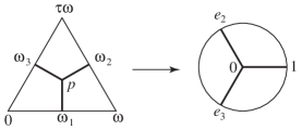
Figure 4.7. Weierstrass $\wp$-function for $g_{2}=0,g_{3}=4$.

A Strebel differential is given by

(4.19) $$q=-\frac{9}{\pi^{2}}\wp(z)(dz)^{2},$$

and the non-compact leaves form a regular hexagonal network, which possesses a $\mathbb{Z}/3\mathbb{Z}$-symmetry (Figure 4.8).

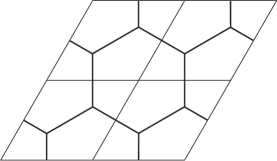
Figure 4.8. A honeycomb.

We note that (4.19) is the pull-back of the building block $q_{0}$ via a map

$$E_{e^{\pi i/3}}\overset{\wp^{3}}{\longrightarrow}\mathbb{P}^{1}.$$

Indeed, we have

$$q=-\frac{9}{\pi^{2}}\wp(z)(dz)^{2}=\frac{1}{4\pi^{2}}\frac{(d\wp^{3})^{2}}{\wp^{3}(1-\wp^{3})}.$$

We can now construct the canonical coordinate system by using the Strebel differential once we give $n$ marked points on a Riemann surface and an $n$-tuple of real numbers. Let $(C,(p_{1},p_{2},\cdots,p_{n}),(a_{1},a_{2},\cdots,a_{n}))$ be the set of data of (4.11), and $q$ the Strebel differential associated with the data. We recall that for every point of a vertical leaf there is a horizontal leaf intersecting perpendicularly at the point (Proposition 4.1). Since the set of compact horizontal leaves of $q$ forms an open dense subset of $C$, which is indeed the disjoint union of punctured open $2$-disks, every vertical leaf of $q$ extends to one of the points $p_{j}$. In particular, a vertical leaf starting at a zero of $q$ should end at one of the poles.

Theorem 4.4.

The set of all vertical leaves that connect zeroes and poles of $q$, together with the cell-decomposition $\square_{q}$ of $C$ by the noncompact horizontal leaves, defines a canonical triangulation $\Delta_{q}$ of $C$.

Proof.

The cell-decomposition $\square_{q}$ of $C$ defined by the noncompact horizontal leaves of $q$ defines a polygonalization of $C$. Each polygon Figure 4.4 has a unique center, which is a pole of $q$. The vertical leaves that connect zeroes and poles supply the edges necessary for a triangulation of each polygon (Figure 4.9). ∎

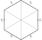
Figure 4.9. Triangulation of a polygon

Let $\Gamma_{q}$ denote a ribbon graph consisting of zeroes of $q$ as vertices and noncompact horizontal leaves of $q$ as edges. By the property of the Strebel differential, we have

(4.20) $$\begin{cases}{\hbox{\raise 1.5pt\hbox{$\chi$}}}(\Gamma_{q})=v(\Gamma_{q})-e(\Gamma_{q})=2-2g\\ b(\Gamma_{q})=n.\end{cases}$$

In particular, the closed surface associated with the ribbon graph $\Gamma_{q}$ is the underlying topological surface of the Riemann surface $C$. For every edge $E$ of $\Gamma_{q}$, there are two triangles of $\Delta_{q}$ that share $E$. Gluing these two triangles along $E$, we obtain a diamond shape as in Figure 4.10. This is the set of all vertical leaves that intersect with $E$. Let $V$ and $V^{\prime}$ be the endpoints of $E$, and give a direction to $E$ from $V$ to $V^{\prime}$. We allow the case that $E$ has only one endpoint. In that case, we assign an arbitrary direction to $E$. For a point $P$ in the triangles, the canonical coordinate

(4.21) $$z=z(P)=\int_{V}^{P}\sqrt{q}$$

maps the diamond shape to a strip

(4.22) $$U_{E}=\{z\in\mathbb{C}\;|\;0<Re(z)<L\}$$

of infinite height and width $L$ in the complex plane, where $L$ is the length of $E$. We identify the open set $U_{E}$ as the union of two triangles on the Riemann surface $C$ by the canonical coordinate $z$ (Figure 4.10). The local expression of $q$ on $U_{E}$ is of course

(4.23) $$q=(dz)^{2}.$$

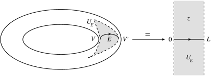
Figure 4.10. Triangulation and a canonical coordinate system of a Riemann surface.

Let the degree of $V$ be $m$. We note that every quadratic differential has an expression

(4.24) $$q=\frac{m^{2}}{4}w^{m-2}(dw)^{2}$$

around a zero of degree $m-2$. So we use (4.24) as the expression of the Strebel differential $q$ on an open neighborhood $U_{V}$ around $V$ with a coordinate $w$ such that $V$ is given by $w=0$. On the intersection

$$U_{E}\cap U_{V},$$

we have

(4.25) $$q=(dz)^{2}=\frac{m^{2}}{4}w^{m-2}(dw)^{2}$$

from (4.23) and (4.24). Solving this differential equation with the initial condition that $z=0$ and $w=0$ define the same point $V$, we obtain the coordinate transform

(4.26) $$w=w(z)=cz^{2/m},$$

where $c$ is an $m$th root of unity. Thus $U_{E}$ and $U_{V}$ are glued on the Riemann surface $C$ in the way described in Figure 4.11.

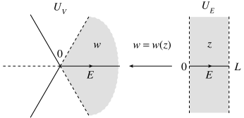
Figure 4.11. Gluing a strip to a neighborhood of a vertex by $w=w(z)=z^{2/3}$.

Since we have

$$\oint\sqrt{q}=a_{j}$$

around a quadratic pole $p_{j}$, we can choose a local coordinate $u$ on an open disk $U_{j}$ centered at $p_{j}$ such that

(4.27) $$q=-\frac{a_{j}^{2}}{4\pi^{2}}\frac{(du)^{2}}{u^{2}}.$$

The coordinate disk $U_{j}$, which is the union of the horizontal leaves that are zero-homotopic to $p_{j}$, can be chosen so that its boundary consists of a collection of edges $E_{1},\cdots,E_{\mu}$ for some $\mu$. Let $z_{k}$ be the canonical coordinate on $U_{E_{k}}$. Equations (4.23) and (4.27) give us a differential equation

(4.28) $$(dz_{k})^{2}=-\frac{a_{j}^{2}}{4\pi^{2}}\frac{(du)^{2}}{u^{2}}.$$

Its solution is given by

(4.29) $$u=u(z_{k})=\gamma e^{2\pi iz_{k}/a_{j}},$$

where $\gamma$ is a constant of integration. Since the edges $E_{1},\cdots,E_{\mu}$ surround the point $p_{j}$, the constant of integration for each $z_{k}$ is arranged so that the solution $u$ of (4.29) covers the entire disk. The precise form of gluing function of open sets $U_{E_{k}}$’s and $U_{j}$ is given by

(4.30) $$u=u(z_{k})={\text{\rm{exp}}}\left(2\pi i\frac{L_{1}+L_{2}+\cdots+L_{k-1}+z_{k}}{L_{1}+L_{2}+\cdots+L_{\mu}}\right),\qquad k=1,2,\cdots,\mu,$$

where the length $L_{k}$ satisfies the condition

$$a_{j}=L_{1}+L_{2}+\cdots+L_{\mu}.$$

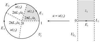
Figure 4.12. Gluing a strip to a neighborhood of a pole by $u=u(z_{1})={\text{\rm{exp}}}(2\pi iz_{1}/a_{j})$.

The open coordinate charts $U_{E}$’s, $U_{V}$’s and $U_{j}$’s cover the whole Riemann surface $C$. We call them the canonical coordinate charts.

Definition 4.5.

The canonical coordinate system of the data

$$(C,(p_{1},p_{2},\cdots,p_{n}),(a_{1},a_{2},\cdots,a_{n}))$$

is the covering

(4.31) $$C=\bigcup_{E}U_{E}\cup\bigcup_{V}U_{V}\cup\bigcup_{j=1}^{n}U_{j}$$

of the Riemann surface $C$ by the canonical coordinate charts, where the union is defined by the gluing functions (4.26) and (4.30).

We note that the canonical coordinate $z$ we have chosen for the strip $U_{E}$ around an edge $E$ depends on the direction of the edge. If we use the opposite direction, then the coordinate changes to

(4.32) $$z\longmapsto L-z,$$

where $L$ is the length of $E$, as before. This change of coordinate does not affect the differential equations (4.25) and (4.28), because

$$(dz)^{2}=(d(L-z))^{2}.$$

5. Combinatorial description of the moduli spaces of Riemann surfaces

We have defined the space of metric ribbon graphs with labeled boundary components by

$$RGB_{g,n}^{\rm{met}}=\coprod_{\Gamma\in RGB_{g,n}}\frac{\mathbb{R}_{+}^{e(\Gamma)}}{{\text{\rm{Aut}}}_{\partial}(\Gamma)}.$$

The Strebel theory defines a map

(5.1) $$\sigma:\mathfrak{M}_{g,n}\times\mathbb{R}_{+}^{n}\longrightarrow RGB_{g,n}^{\text{met}},$$

where $\mathfrak{M}_{g,n}$ is the moduli space of Riemann surfaces of genus $g$ with $n$ ordered marked points. In what follows, we prove that the map $\sigma$ is bijective. The case of $(g,n)=(1,1)$ is in many ways exceptional. For $(g,n)=(0,3)$, all Strebel differentials are explicitly computable. Thus we can construct the identification map

$$\mathfrak{M}_{0,3}\times\mathbb{R}_{+}^{3}=RGB_{0,3}^{\text{met}}$$

directly. This topic is studied at the end of this section. We also examine the orbifold covering $RGB_{0,3}^{\rm{met}}\rightarrow RG_{0,3}^{\rm{met}}$ there.

The product group $\mathbb{R}_{+}^{n}$ acts naturally on $\mathfrak{M}_{g,n}\times\mathbb{R}_{+}^{n}$. Therefore it acts on the space $RGB_{g,n}^{\rm{met}}$ through the bijection $\sigma$. However, the $\mathbb{R}_{+}^{n}$-action on $RGB_{g,n}^{\text{met}}$ is complicated. We give an example in this section which shows that the action does not preserve the rational cells.

Theorem 5.1.

There is a natural bijection

$$\mathfrak{M}_{g,n}\times\mathbb{R}_{+}^{n}=RGB_{g,n}^{\text{met}}.$$

Proof.

The proof breaks down into three steps. In Step 1, we construct a map

(5.2) $$\coprod_{\Gamma\in RGB_{g,n}}\mathbb{R}_{+}^{e(\Gamma)}\longrightarrow\mathfrak{M}_{g,n}\times\mathbb{R}_{+}^{n}.$$

We then prove that the map descends to

(5.3) $$\beta:RGB_{g,n}^{\text{met}}\longrightarrow\mathfrak{M}_{g,n}\times\mathbb{R}_{+}^{n}$$

by considering the action of the graph automorphism groups preserving the boundary order in Step 2. From the construction of Step 1 we will see that $\beta$ is a right-inverse of the map $\sigma$ of (5.1), i.e., $\sigma\circ\beta$ is the identity of $RGB_{g,n}^{\text{met}}$. In Step 3 we prove that $\beta$ is also a left-inverse of the map $\sigma$.

Step 1.

Our starting point is a metric ribbon graph $\Gamma_{\rm{met}}$ with labeled boundary components. We label all edges, and give an arbitrary direction to each edge. To each directed edge $\overrightarrow{E}$ of $\Gamma_{\rm{met}}$, we assign a strip

$$U_{\overrightarrow{E}}=\{z\in\mathbb{C}\;|\;0<Re(z)<L\}$$

of infinite length and width $L$, where $L$ is the length of $E$ (see Figure 5.1). The open real line segment $(0,L)\subset U_{\overrightarrow{E}}$ is identified with the edge $\overrightarrow{E}$. The strip $U_{\overrightarrow{E}}$ has a complex structure defined by the coordinate $z$, and a holomorphic quadratic differential $(dz)^{2}$ on it. Every horizontal leaf of the foliation defined by this quadratic differential is a horizontal line of length $L$. If we use the opposite direction of $\overrightarrow{E}$, then $U_{\overrightarrow{E}}$ should be rotated $180^{\circ}$ about the real point $L/2$, and the coordinate is changed to $L-z$.

Figure 5.1. A strip of infinite length with horizontal leaves.

Let $V$ be a degree $m$ vertex of $\Gamma$. There are $m$ half-edges attached to $V$, although some of them may belong to the same edge. Let $1,2,\cdots,m$ be the cyclic order of the half-edges chosen at $V$. We give a direction to each edge by defining the positive direction to be the one coming out from $V$, and name the edges $\overrightarrow{E}_{1},\overrightarrow{E}_{2},\cdots,\overrightarrow{E}_{m}$. If an edge goes out as a half-edge number $j$ and comes back as another half-edge number $k$, then we use the convention that $\overrightarrow{E}_{j}=\overleftarrow{E}_{k}$, where $\overleftarrow{E}_{k}$ denotes the edge $E_{k}$ with the opposite direction. We denote by $L_{j}$ the length of $E_{j}$.

Let us place the vertex $V$ at the origin of the $w$-plane. We glue a neighborhood of the boundary point $0$ of each of the strips $U_{\overrightarrow{E}_{1}},\cdots,U_{\overrightarrow{E}_{m}}$ together on the $w$-plane by

(5.4) $$w=e^{2\pi i(j-1)/m}z_{j}^{2/m},\qquad j=1,2,\cdots,m.$$

An open neighborhood $U_{V}$ of $w=0$ is covered by this gluing, if we include the boundary of each $U_{\overrightarrow{E}_{j}}$. It follows from (5.4) that the expression of the quadratic differential $(dz_{j})^{2}$ changes into

(5.5) $$(dz_{j})^{2}=\frac{m^{2}}{4}w^{m-2}(dw)^{2}$$

in the $w$-coordinate for every $j$. So we define a holomorphic quadratic differential $q$ on $U_{V}$ by (5.5). Note that $q$ has a zero of degree $m-2$ at $w=0$. At least locally on $U_{V}$, the horizontal leaves of the foliation defined by $q$ that have $V$ as a boundary point coincide with the image of the edges $E_{1},\cdots,E_{m}$ via (5.4).

Next, let us consider the case when edges $\overrightarrow{E}_{1},\overrightarrow{E}_{2},\cdots,\overrightarrow{E}_{h}$ form an oriented boundary component $B$ of $\Gamma$, where the direction of $\overrightarrow{E}_{k}$ is chosen to be compatible with the orientation of $B$. Here again we allow that some of the edges are actually the same, with the opposite direction. As before, let $L_{k}$ be the length of $E_{k}$, and put

(5.6) $$a_{B}=L_{1}+L_{2}+\cdots L_{h}.$$

This time we glue the upper half of the strips $U_{\overrightarrow{E}_{1}},\cdots,U_{\overrightarrow{E}_{h}}$ (or the lower half, if the edge has the opposite direction) into the unit disk of the $u$-plane by

(5.7) $$u={\text{\rm{exp}}}\left(\frac{2\pi i}{a_{B}}(L_{1}+L_{2}+\cdots+L_{k-1}+z_{k})\right),\qquad k=1,2,\cdots,h.$$

We note that the entire unit disk on the $u$-plane, which we denote by $U_{B}$, is covered by this gluing, if the boundary lines of the strips are included.

It follows from this coordinate transform that

(5.8) $$(dz_{k})^{2}=-\frac{a_{B}^{2}}{4\pi^{2}}\frac{(du)^{2}}{u^{2}}.$$

Thus the holomorphic quadratic differential $q$ naturally extends to a meromorphic quadratic differential on the union

$$U_{B}\cup\bigcup_{k=1}^{h}U_{\overrightarrow{E}_{k}}$$

which has a pole of order 2 at $u=0$ with a negative real coefficient. The horizontal leaves of the foliation defined by $q$ are concentric circles that are centered at $u=0$, which correspond to the horizontal lines on $U_{\overrightarrow{E}_{k}}$ through (5.7). Note that the length of a compact horizontal leaf around $u=0$ is always $a_{B}$.

Now define a compact Riemann surface $C(\Gamma_{\rm{met}})$ by gluing all the $U_{V}$’s, $U_{B}$’s and the strips $U_{\overrightarrow{E}}$’s by (5.4) and (5.7):

(5.9) $$C(\Gamma_{\rm{met}})=\bigcup_{V:\text{ vertex of }\Gamma}U_{V}\cup\bigcup_{E:\text{ edge of }\Gamma}U_{\overrightarrow{E}}\cup\bigcup_{\begin{subarray}{c}B:\text{ boundary}\\ \text{component of }\Gamma\end{subarray}}U_{B}.$$

Since there are two directions for every edge $E$, both the upper half part and the lower half part of a strip $U_{\overrightarrow{E}}$ are included in the union of all $U_{B}$’s. Thus the union (5.9) is compact. The Riemann surface $C(\Gamma_{\rm{met}})$ has $n=b(\Gamma)$ marked points each of which is the center of the unit disk $U_{B}$. The ordering of the boundary components of the ribbon graph determines an ordering of the marked points on the Riemann surface. Attached to each marked point we have a positive real number $a_{B}$. The Riemann surface also comes with a meromorphic quadratic differential whose local expressions are given by $(dz_{j})^{2}$, (5.5), and (5.8). It is a Strebel differential on $C(\Gamma_{\rm{met}})$. The metric ribbon graph corresponding to this Strebel differential is, by construction, exactly the original graph $\Gamma_{\rm{met}}$, which has a natural ordering of the boundary components. Thus we have constructed a map (5.2).

Step 2.

Let us consider the effect of a graph automorphism $f\in{\text{\rm{Aut}}}_{\partial}(\Gamma)$ on (5.9). Let $p_{1},\cdots,p_{n}$ be the marked points of $C(\Gamma_{\rm{met}})$, and $a_{1},\cdots,a_{n}$ the corresponding positive numbers. We denote by $E_{1},\cdots,E_{e}$ the edges of $\Gamma$, and by $U_{\overrightarrow{E}_{1}},\cdots,U_{\overrightarrow{E}_{e}}$ the corresponding strips with a choice of direction. Then the union of the closures of these strips cover the Riemann surface minus the marked points:

$$C(\Gamma_{\rm{met}})\setminus\{p_{1},\cdots,p_{n}\}=\bigcup_{j=1}^{e}\overline{U}_{\overrightarrow{E}_{j}}.$$

A graph automorphism $f:\Gamma_{\rm{met}}\rightarrow\Gamma_{\rm{met}}$ induces a permutation of edges and flip of directions, and hence a permutation of strips $U_{\overrightarrow{E}_{1}},\cdots,U_{\overrightarrow{E}_{e}}$ and a change of coordinate $z_{j}$ to $L_{j}-z_{j}$. If $f$ fixes a vertex $V$ of degree $m$, then it acts on $U_{V}$ by rotation of angle an integer multiple of $2\pi/m$, which is a holomorphic automorphism of $U_{V}$. The permutation of vertices induced by $f$ is a holomorphic transformation of the union of $U_{V}$’s. Since $f$ preserves the boundary components of $\Gamma$, it does not permute $U_{B}$’s, but it may rotate each $U_{B}$ following the effect of the permutation of edges. In this case, the origin of $U_{B}$, which is one of the marked points, is fixed, and the orientation of the boundary is also fixed. Thus the graph automorphism induces a holomorphic automorphism of $C(\Gamma_{\rm{met}})\setminus\{p_{1},\cdots,p_{n}\}$. This holomorphic automorphism preserves the ordering of the marked points. Thus we conclude that (5.2) descends to a map $\beta$ which satisfies $\sigma\circ\beta=id$.

Step 3.

We still need to show that $\beta\circ\sigma$ is the identity map of $\mathfrak{M}_{g,n}\times\mathbb{R}_{+}^{n}$, but this is exactly what we have shown in the previous section.

This completes the proof of Theorem 5.1. ∎

Example 5.1.

Let us consider the complex projective line $\mathbb{P}^{1}$ with three ordered marked points, to illustrate the equality

$$\mathfrak{M}_{0,3}\times\mathbb{R}_{+}^{3}=RGB_{0,3}^{\text{met}}$$

and the covering map

$$RGB_{0,3}^{\text{met}}\longrightarrow RG_{0,3}^{\text{met}}.$$

The holomorphic automorphism group of $\mathbb{P}^{1}$ is $PSL(2,\mathbb{C})$, which acts on $\mathbb{P}^{1}$ triply transitively. Therefore, we have a biholomorphic equivalence

$$(\mathbb{P}^{1},(p_{1},p_{2},p_{3}))\cong(\mathbb{P}^{1},(0,1,\infty)).$$

In other words, $\mathfrak{M}_{0,3}$ is just a point. Choose a triple $(a_{0},a_{1},a_{\infty})$ of positive real numbers. The unique Strebel differential is given by

(5.10) $$q=-\frac{1}{4\pi^{2}}\left(a\left(\frac{dx}{x}\right)^{2}+b\left(\frac{dx}{1-x}\right)^{2}+c\left(\frac{dx}{x(1-x)}\right)^{2}\right),$$

where

$$\begin{cases}a=\frac{1}{2}\left(a_{0}^{2}+a_{\infty}^{2}-a_{1}^{2}\right)\\ b=\frac{1}{2}\left(a_{1}^{2}+a_{\infty}^{2}-a_{0}^{2}\right)\\ c=\frac{1}{2}\left(a_{0}^{2}+a_{1}^{2}-a_{\infty}^{2}\right).\end{cases}$$

The behavior of the foliation of the Strebel differential $q$ depends on the discriminant

$$ab+bc+ca=\frac{1}{4}\left(a_{0}+a_{1}+a_{\infty}\right)\left(a_{0}+a_{\infty}-a_{1}\right)\left(a_{1}+a_{\infty}-a_{0}\right)\left(a_{0}+a_{1}-a_{\infty}\right).$$

Case 1.

$ab+bc+ca>0$. The graph is trivalent with two vertices and three edges, as given in Figure 5.2. The two vertices are located at

(5.11) $$\frac{a\pm i\sqrt{ab+bc+ca}}{a+b},$$

and the length of edges $L_{1}$, $L_{2}$ and $L_{3}$ are given by

(5.12) $$\begin{cases}L_{1}=\frac{1}{2}\left(a_{0}+a_{\infty}-a_{1}\right)=\frac{1}{2}\left(\sqrt{a+c}+\sqrt{a+b}-\sqrt{b+c}\right)\\ L_{2}=\frac{1}{2}\left(a_{1}+a_{\infty}-a_{0}\right)=\frac{1}{2}\left(\sqrt{b+c}+\sqrt{a+b}-\sqrt{a+c}\right)\\ L_{3}=\frac{1}{2}\left(a_{0}+a_{1}-a_{\infty}\right)=\frac{1}{2}\left(\sqrt{a+c}+\sqrt{b+c}-\sqrt{a+b}\right).\end{cases}$$

Note that positivity of $L_{1},L_{2}$ and $L_{3}$ follows from $ab+bc+ca>0$. The space of metric ribbon graphs with ordered boundary in this case is just $\mathbb{R}_{+}^{3}$ because there is only one ribbon graph with boundary order of this type and the only graph automorphism that preserves the boundary order is the identity transformation.

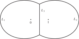
Figure 5.2. The critical horizontal leaves of the Strebel differential for $ab+bc+ca>0$.

The natural $\mathfrak{S}_{3}$-action on the space of $(a_{0},a_{1},a_{\infty})$ induces faithful permutations of $L_{1}$, $L_{2}$ and $L_{3}$ through (5.12). The geometric picture can be easily seen from Figure 5.3. The normal subgroup $\mathbb{Z}/3\mathbb{Z}$ of $\mathfrak{S}_{3}$ acts on $\mathbb{P}^{1}$ as rotations about the axis connecting the north pole and the south pole, where the poles of Figure 5.3 represent the zeroes (5.11) of the Strebel differential. Note that the three non-compact leaves intersect at a zero of $q$ with $120^{\circ}$ angles. The action of the whole group $\mathfrak{S}_{3}$ is the same as the dihedral group $D_{3}$ action on the triangle $\triangle 01\infty$. As a result, $\mathfrak{S}_{3}$ acts faithfully on $(L_{1},L_{2},L_{3})$ as its group of permutations.

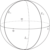
Figure 5.3. A degree $3$ graph on a sphere.

The special case $(a_{0},a_{1},a_{\infty})=(2,2,2)$ is of particular interest. The Strebel differential (5.10) is the pull-back of the building block $q_{0}$ of (4.12) via a rational map

(5.13) $$\zeta=\frac{4(x^{2}-x+1)^{3}}{27x^{2}(1-x)^{2}},$$

and the ribbon graph Figure 5.2 is the inverse image of the interval $[0,1]$ of this map.

Case 2.

$ab+bc+ca=0$. There are three ribbon graphs with labeled boundary components in this case, whose underlying graph has 1 vertex of degree $4$ and two edges (Figure 5.4). The vertex is located at $a/(a+b)$. Each of the three graphs corresponds to one of the three factors, $\left(a_{0}+a_{\infty}-a_{1}\right)$, $\left(a_{1}+a_{\infty}-a_{0}\right)$, and $\left(a_{0}+a_{1}-a_{\infty}\right)$, of the discriminant being equal to $0$. For example, when $\left(a_{0}+a_{1}-a_{\infty}\right)=0$, and the lengths of the edges are given by

$$\begin{cases}L_{1}=a_{0}=\sqrt{a+c}\\ L_{2}=a_{1}=\sqrt{b+c}\\ L_{3}=0.\end{cases}$$

The $\mathfrak{S}_{3}$-action on $(a_{0},a_{1},a_{\infty})$ interchanges the three types of ribbon graphs with boundary order in Case 2. The automorphism group of the ribbon graph of Case 2 is $\mathbb{Z}/2\mathbb{Z}$, and only the identity element preserves the boundary order.

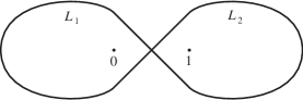
Figure 5.4. Case $ab+bc+ca=0$.

Case 3.

$ab+bc+ca<0$. The underlying graph is of degree $3$ with two vertices and three edges, but the topological type is different from Case 1 (Figure 5.5). The two vertices are on the real axis located at

$$\frac{a\pm\sqrt{-(ab+bc+ca)}}{a+b}.$$

There are again three different ribbon graphs with ordered boundary, each of which corresponds to one of the three factors of the discriminant being negative. For example, if $\left(a_{0}+a_{1}-a_{\infty}\right)<0$, then the length of edges are given by

$$\begin{cases}L_{1}=a_{0}=\sqrt{a+c}\\ L_{2}=a_{1}=\sqrt{b+c}\\ L_{3}=\frac{1}{2}\left(-a_{0}-a_{1}+a_{\infty}\right)=\frac{1}{2}\left(-\sqrt{a+c}-\sqrt{b+c}+\sqrt{a+b}\right).\end{cases}$$

$L_{3}$ is positive because $ab+bc+ca<0$.

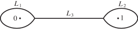
Figure 5.5. Case $ab+bc+ca<0$.

In Case 2 and Case 3, the automorphism group of the ribbon graph without ordered boundaries is $\mathbb{Z}/2\mathbb{Z}$. In every case, we can make the length of edges arbitrary by a suitable choice of $(a_{0},a_{1},a_{\infty})$. The discriminant $ab+bc+ca$ divides the space $\mathbb{R}_{+}^{3}$ of triples $(a_{0},a_{1},a_{\infty})$ into 7 pieces: 3 copies of $\mathbb{R}_{+}^{3}$ along the $a_{0}$, $a_{1}$ and $a_{\infty}$ axes where the discriminant is negative, the center piece of $\mathbb{R}_{+}^{3}$ characterized by positivity of the discriminant, and 3 copies of $\mathbb{R}_{+}^{2}$ separating the 4 chambers that correspond to the zero points of the discriminant (Figure 5.6):

(5.14) $$\mathbb{R}_{+}^{3}=\mathbb{R}_{+}^{3}\coprod\mathbb{R}_{+}^{2}\coprod\mathbb{R}_{+}^{2}\coprod\mathbb{R}_{+}^{2}\coprod\mathbb{R}_{+}^{3}\coprod\mathbb{R}_{+}^{3}\coprod\mathbb{R}_{+}^{3}.$$

The product group $\mathbb{R}_{+}^{3}$ acts on the space of $(a_{0},a_{1},a_{\infty})$ by multiplication, but the action does not preserve the canonical rational cell-decomposition of $RGB_{0,3}^{\rm{met}}$. Indeed, this action changes the sign of the discriminant.

The three $\mathbb{R}_{+}^{3}$’s along the axes are equivalent under the $\mathfrak{S}_{3}$-action on the space of $(a_{0},a_{1},a_{\infty})$, and each has a $\mathfrak{S}_{2}$-symmetry. The three walls separating the chambers are also equivalent under the $\mathfrak{S}_{3}$-action, and again have the same symmetry. Only the central chamber is acted on by the full $\mathfrak{S}_{3}$. Thus we have

(5.15) $$\begin{CD}\mathbb{R}_{+}^{3}@=\mathbb{R}_{+}^{3}\coprod\mathbb{R}_{+}^{2}\coprod\mathbb{R}_{+}^{2}\coprod\mathbb{R}_{+}^{2}\coprod\mathbb{R}_{+}^{3}\coprod\mathbb{R}_{+}^{3}\coprod\mathbb{R}_{+}^{3}\\ @V{}V{}V@V{}V{}V\\ \mathbb{R}_{+}^{3}/\mathfrak{S}_{3}@=\mathbb{R}_{+}^{3}/\mathfrak{S}_{3}\coprod\mathbb{R}_{+}^{2}/\mathfrak{S}_{2}\coprod\mathbb{R}_{+}^{3}/\mathfrak{S}_{2}.\end{CD}$$

Figure 5.6. Partition of $RGB_{0,3}^{\rm{met}}=\mathbb{R}_{+}^{3}$.

The multiplicative group $\mathbb{R}_{+}$ acts naturally on the ribbon graph complexes $RG_{g,n}^{\rm{met}}$ and $RGB_{g,n}^{\rm{met}}$ by the multiplication of all the edge lengths by a constant. Since the graph automorphism groups ${\text{\rm{Aut}}}(\Gamma)$ and ${\text{\rm{Aut}}}_{\partial}(\Gamma)$ act on the edge space $\mathbb{R}_{+}^{e(\Gamma)}$ through a permutation of coordinate axes, the multiplicative $\mathbb{R}_{+}$-action and the action of the graph automorphism groups commute. Therefore, we have well-defined quotient complexes $RG_{g,n}^{\rm{met}}/\mathbb{R}_{+}$ and $RGB_{g,n}^{\rm{met}}/\mathbb{R}_{+}$. Since $\mathbb{R}_{+}^{e(\Gamma)}$ is a cone over the $(e(\Gamma)-1)$-dimensional regular $e(\Gamma)$-hyperhedron $\Delta(123\cdots e(\Gamma))$ and since the graph automorphism groups act on the hyperhedron, the quotient of each rational cell is a rational simplex

$$\frac{\Delta(123\cdots e(\Gamma))}{{\text{\rm{Aut}}}(\Gamma)}.$$

Thus the quotient complexes $RG_{g,n}^{\rm{met}}/\mathbb{R}_{+}$ and $RGB_{g,n}^{\rm{met}}/\mathbb{R}_{+}$ are rational simplicial complexes.

These quotient complexes are orbifolds modeled on

$$\frac{X_{\succeq\Gamma}^{\rm{met}}/\mathbb{R}_{+}}{G},$$

where $G$ denotes either ${\text{\rm{Aut}}}(\Gamma)$ or ${\text{\rm{Aut}}}_{\partial}(\Gamma)$. From (3.14), we have

(5.16) $$\frac{X_{\succeq\Gamma}^{\rm{met}}/\mathbb{R}_{+}}{{\text{\rm{Aut}}}(\Gamma)}=\frac{\Delta(123\cdots e(\Gamma))\times\mathbb{R}^{\rm{codim}(\Gamma)}}{{\text{\rm{Aut}}}(\Gamma)}.$$

Since $\Delta(123\cdots e(\Gamma))$ is homeomorphic to $\mathbb{R}_{+}^{e(\Gamma)-1}$, the quotient complexes are topological orbifolds.

On the moduli space $\mathfrak{M}_{g,n}\times\mathbb{R}_{+}^{n}$, the multiplicative group $\mathbb{R}_{+}$ acts on the space of $n$-tuples $\mathbb{R}_{+}^{n}$ through the multiplication of constants. The action has no effect on $\mathfrak{M}_{g,n}$. Thus we have the quotient space

$$\frac{\mathfrak{M}_{g,n}\times\mathbb{R}_{+}^{n}}{\mathbb{R}_{+}}=\mathfrak{M}_{g,n}\times\Delta(123\cdots n).$$

The bijection of Theorem 5.1 is equivariant under the $\mathbb{R}_{+}$-action, and we have

(5.17) $$\mathfrak{M}_{g,n}\times\Delta(123\cdots n)=\coprod_{\Gamma\in RGB_{g,n}}\frac{\Delta(123\cdots e(\Gamma))}{{\text{\rm{Aut}}}_{\partial}(\Gamma)}.$$

This gives us an orbifold realization of the space $\mathfrak{M}_{g,n}\times\Delta(123\cdots n)$ as a rational simplicial complex. When $n=1$, the space $\Delta(1)$ consists of just a point. Therefore, we have a rational simplicial complex realization

(5.18) $$\mathfrak{M}_{g,1}=\coprod_{\Gamma\in RG_{g,1}}\frac{\Delta(123\cdots e(\Gamma))}{{\text{\rm{Aut}}}(\Gamma)}.$$

6. Belyi maps and algebraic curves defined over $\overline{\mathbb{Q}}$

We have shown that a metric ribbon graph defines a Riemann surface and a Strebel differential on it. One can ask a question: when does this Riemann surface have the structure of an algebraic curve defined over $\overline{\mathbb{Q}}$? Using Belyi’s theorem [1], we can answer this question.

Definition 6.1.

Let $C$ be a nonsingular Riemann surface. A Belyi map is a holomorphic map

$$f:C\longrightarrow\mathbb{P}^{1}$$

that is ramified only at $0$, $1$ and $\infty$.

Theorem 6.2 (Belyi’s Theorem [1]).

A nonsingular Riemann surface $C$ has the structure of an algebraic curve defined over $\overline{\mathbb{Q}}$ if and only if there is a Belyi map onto $\mathbb{P}^{1}$.

Corollary 6.3.

A nonsingular Riemann surface $C$ has the structure of an algebraic curve defined over $\overline{\mathbb{Q}}$ if and only if there is a Belyi map

$$f:C\longrightarrow\mathbb{P}^{1}$$

such that the ramification degrees over $0$ and $1$ are $3$ and $2$, respectively. Such a Belyi map is called trivalent.

Proof.

Let $C$ be an algebraic curve over $\overline{\mathbb{Q}}$ and $h:C\longrightarrow\mathbb{P}^{1}$ a Belyi map. Then the composition $f=\phi\circ h$ of $h$ and

$$\phi:\mathbb{P}^{1}\owns x\longmapsto\zeta=\frac{4(x^{2}-x+1)^{3}}{27x^{2}(1-x)^{2}}\in\mathbb{P}^{1}$$

of (5.13) gives a trivalent Belyi map. We first note that

$$\frac{d\zeta}{dx}=-\frac{4(x-2)(x+1)(2x-1)(x^{2}-x+1)^{2}}{27x^{3}(1-x)^{3}}.$$

Thus the ramification points of $\phi$ are $x=-1$, $x=1/2$, $x=2$, and

$$x=\frac{1\pm i\sqrt{3}}{2}.$$

The critical values of $\phi$ are

$$\phi(-1)=\phi(1/2)=\phi(2)=1$$

and

$$\phi\left(\frac{1\pm i\sqrt{3}}{2}\right)=0,$$

and the ramification degrees at $1$ and $0$ are $2$ and $3$, respectively. $\phi$ sends $\{0,1,\infty\}$ to $\infty$, at which it is also ramified. Since $h$ is not ramified at $e^{\pm i\pi/3}$, $-1$, $1/2$, or $2$, the composed map $f$ is ramified only at $0$, $1$, and $\infty$ with the desired ramification degrees.

The inverse image of the interval $[0,1]$ via $\phi$ is a ribbon graph of Figure 6.1. This graph is obtained by adjoining two circles of radius $1$ that are centered at $0$ and $1$ together with a common boundary at $1/2$. ∎

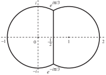
Figure 6.1. The inverse image of $[0,1]$ via $\zeta=\frac{4(x^{2}-x+1)^{3}}{27x^{2}(1-x)^{2}}$. It is obtained by joining two circles of radius $1$ at $1/2$.

Definition 6.4.

A child’s drawing, or Grothendieck’s dessin d’enfant, is the inverse image of the line segment $[0,1]$ by a Belyi map.

Theorem 6.5.

Let $\Gamma_{\rm{met}}$ be a metric ribbon graph with no vertices of degree less than $3$. It gives rise to an algebraic curve defined over $\overline{\mathbb{Q}}$ if all the edges have the same length, which can be chosen to be $1$. The metric ribbon graph determines a unique Belyi map

$$f:C(\Gamma_{\rm{met}})\longrightarrow\mathbb{P}^{1}$$

such that the child’s drawing associated with $f$ is the edge refinement of $\Gamma_{\rm{met}}$. The Strebel differential $q$ on $C(\Gamma_{\rm{met}})$ is the pull-back of the building block $q_{0}$ of (4.12) via the Belyi map, i.e.,

$$q=f^{*}\left(\frac{(d\zeta)^{2}}{4\pi^{2}\zeta(1-\zeta)}\right).$$

Conversely, every nonsingular algebraic curve over $\overline{\mathbb{Q}}$ can be constructed from a trivalent metric ribbon graph with edge length $1$.

Proof.

Let $\Gamma_{\rm{met}}$ be a metric ribbon graph whose edges all have length $1$, $C(\Gamma_{\rm{met}})$ be the Riemann surface defined by the metric ribbon graph, and $q$ the Strebel differential on $C(\Gamma_{\rm{met}})$ whose noncompact leaves are $\Gamma_{\rm{met}}$. We take the canonical triangulation $\Delta_{q}$ of Theorem 4.4 and the canonical coordinate system of Definition 4.5.

For every edge $E$ of $\Gamma_{\rm{met}}$, we define a map from a triangle with base $E$ into $\mathbb{P}^{1}$ as follows. The triangle can be identified with the upper half of the strip of Figure 5.1. So we define

(6.1) $$\{z\in\mathbb{C}\;|\;0\leq Re(z)\leq 1,Im(z)\geq 0\}\owns z\longmapsto\zeta=\sin^{2}(\pi z)\in\mathbb{P}^{1}.$$

We note that (6.1) is equivalent to

(6.2) $$(dz)^{2}=q_{0}=\frac{1}{4\pi^{2}}\frac{(d\zeta)^{2}}{\zeta(1-\zeta)}.$$

We wish to show that this map consistently extends to a holomorphic Belyi map

$$f:C(\Gamma_{\rm{met}})\longrightarrow\mathbb{P}^{1}.$$

The map (6.1) extends to the whole strip in an obvious way. The point $z=1/2$ is mapped to $\zeta=1$, at which the map is ramified with ramification degree $2$.

At a vertex $V$ to which $E$ is incident, the canonical coordinate is given by

$$w=2^{2\pi ik/m}z^{2/m}$$

as in (5.4), where $m$ is the degree of $V$ and $k$ is an integer. In terms of the $w$-coordinate, the map (6.1) is given by

$$\zeta=\sin^{2}(\pm\pi w^{m/2})=\pi^{2}w^{m}+\cdots.$$

This expression does not depend on the choice of an edge attached to $V$, hence the map (6.1) extends consistently to a neighborhood of $V$. The map is ramified at $\zeta=0$ with local ramification degree $m$.

Finally, let us consider a boundary component of $\Gamma_{\rm{met}}$ consisting of $k$ edges. From (5.7), we have a local coordinate $u$ on the boundary disk that is given by

$$u={\text{\rm{exp}}}\left(\frac{2\pi i(j+z)}{k}\right),$$

where $j$ is an integer. Then

$$z=\frac{k}{2\pi i}\log u-j.$$

Noting that

$$\sin^{2}(x)=-\frac{e^{2ix}+e^{-2ix}-2}{4},$$

we have

(6.3) $$\zeta=-\frac{1}{4}(u^{k}+u^{-k}-2).$$

This map sends $u=0$ to $\zeta=\infty$, and is independent of the choice of edge around $u=0$ and branch of the logarithm function. The map (6.3) is equivalent to the relation

$$-\frac{k^{2}}{4\pi^{2}}\frac{(du)^{2}}{u^{2}}=\frac{(d\zeta)^{2}}{4\pi^{2}\zeta(1-\zeta)}=q_{0}.$$

We have thus shown that the map (6.1) extends to a holomorphic map $f$ from the whole Riemann surface $C(\Gamma_{\rm{met}})$ onto $\mathbb{P}^{1}$ that is ramified only at $0,1,\infty$. The unique Strebel differential $q$ is given by $f^{*}q_{0}$.

Conversely, let $C$ be a nonsingular algebraic curve defined over $\overline{\mathbb{Q}}$. Let

$$f:C\longrightarrow\mathbb{P}^{1}$$

be a trivalent Belyi map. Then the inverse image of the interval $[0,1]$ via $f$ is the edge refinement of a trivalent metric ribbon graph on $C$ whose edge length is $1$ everywhere. It is the union of noncompact leaves of the Strebel differential $f^{*}q_{0}$ on $C$. Starting from this child’s drawing, we recover the complex structure of $C$. ∎

We have already given two examples of genus $1$ in Section 4 and one example of genus $0$ in Section 5.

Theorem 6.5 does not completely characterize which metric ribbon graphs correspond to algebraic curves defined over $\overline{\mathbb{Q}}$. Furthermore, in Grothendieck’s dessin d’enfant graphs which have vertices of degree 2 and 1 also appear. It is possible to incorporate the vertices of degree 2 coming from these child’s drawings in terms of usual ribbon graphs (those with no vertices having degree less than 3) by sharpening the statement of the theorem as follows.

Corollary 6.6.

Let $\Gamma_{\rm{met}}$ be a metric ribbon graph, such that the ratios of the lengths of its edges are all rational, (so they can be chosen to be positive integers). Then there is a unique Belyi map $f:C(\Gamma_{\rm{met}})\longrightarrow\mathbb{P}^{1}$, such that if $\tilde{\Gamma}_{\rm{met}}$ is the metric graph obtained by replacing each edge of length $n$ with $n$ edges of length 1 by inserting $n-1$ vertices of degree 2 in the edge, then the child’s drawing associated with $f$ is the edge refinement of $\tilde{\Gamma}_{\rm{met}}$. In addition, the Strebel differential $q$ on $C(\Gamma_{\rm{met}})$ is given by $q=f^{*}q_{0}$.

Proof.

Essentially, the only change in the proof of the theorem needed is to replace the map $\sin^{2}(\pi z)$ from the strip associated with an edge $E$ with the map $\sin^{2}(n\pi z)$. This will add $n-1$ additional zeros on the edge, each with ramification degree $2$. ∎

To obtain the complete classification of metric ribbon graphs which correspond to algebraic curves defined over $\overline{\mathbb{Q}}$, we shall have to consider ribbon graphs which have vertices of degree 1. In the theory of Strebel differentials, vertices of degree 1 correspond to poles of order 1 of the quadratic differential. There is a uniqueness theorem concerning Strebel differentials which have poles of order at most 2 as well. See Theorem 7.6 in [5] for a precise statement of the result.

For our purposes, we really only need to address the question of how to construct a Riemann surface corresponding to a metric ribbon graph. The reader can easily verify that the construction of a Riemann surface corresponding to a metric ribbon graph given in Theorem 5.1 still applies when we allow the graphs to have vertices of degree 1 or 2. Furthermore, the construction also yields a quadratic differential, which has poles of order 1 for vertices of degree 1, and neither a pole nor a zero for vertices of degree 2 (although they will lie on the critical trajectories).

The same methods as in Theorem 6.5 allow one to construct a Belyi map from the Riemann surface corresponding to this more general type of ribbon graph, by associating the metric ribbon graph with all edges having length 1 to the graph. Putting this all together, we come up with the following.

Theorem 6.7.

There is a one to one correspondence between the following:

1. The set of isomorphism classes of ribbon graphs.

2. The set of isomorphism classes of child’s drawings.

3. The set of isomorphism classes of Belyi maps.

This correspondence is given as follows. A ribbon graph $\Gamma$ corresponds to a metric ribbon graph $\Gamma_{{\rm met}}$ with all edges having length 1, giving rise to a Riemann surface $C(\Gamma_{{\rm met}})$ and a Strebel differential $q$ which is the pullback of the quadratic differential $q_{0}$ by the unique Belyi map from $C(\Gamma_{{\rm met}})$ to $\mathbb{P}^{1}$ whose associated child’s drawing is the edge refinement of $\Gamma_{\rm met}$. Moreover, this correspondence between ribbon graphs and Belyi maps agrees with the Grothendieck correspondence.

Grothendieck’s use of the terminology child’s drawing to illustrate the relationship between graphs and algebraic curves emphasizes how strange and beautiful it is that a deep area of mathematics can be described in such simple terms. In our construction, we have shown how to take a Child’s drawing, associate a metric ribbon graph to it, construct a Riemann surface equipped with a quadratic differential, as well as a Belyi map from this surface to $\mathbb{P}^{1}$. It is amazing how much information is concealed within such a simple picture.

References

- [1] G. V. Belyi, On galois extensions of a maximal cyclotomic fields, Math. U.S.S.R. Izvestija 14 (1980), 247–256.
- [2] Fredderick P. Gardiner, Teichmüller theory and quadratic differentials, John Wiley & Sons, 1987.
- [3] John L. Harer, The cohomology of the moduli space of curves, in Theory of Moduli, Montecatini Terme, 1985 (Edoardo Sernesi, ed.), Springer-Verlag, 1988, pp. 138–221.
- [4] John L. Harer and Don Zagier, The Euler characteristic of the moduli space of curves, Inventiones Mathematicae 85 (1986), 457–485.
- [5] Eduard Looijenga, Cellular decompositions of compactified moduli spaces of pointed curves, in Moduli Space of Curves (R. H. Dijkgraaf et al., ed.), Birkhaeuser, 1995, pp. 369–400.
- [6] Motohico Mulase, Asymptotic analysis of a hermitian matrix integral, International Journal of Mathematics 6 (1995), 881–892.
- [7] Robert C. Penner, Perturbation series and the moduli space of Riemann surfaces, Journal of Differential Geometry 27 (1988), 35–53.
- [8] Giovanni Sansone and Johan Gerretsen, Lectures on the theory of functions of a complex variable, volume i and ii, Wolters-Noordhoff Publishing, 1960, 1969.
- [9] Ichiro Satake, The Gauss-Bonnet theorem for V-manifold, Journal of the Mathematical Society of Japan 9 (1957), 464–492.
- [10] Leila Schneps, The grothendieck theory of dessins d’enfants, London Mathematical Society Lecture Notes Series, vol. 200, 1994.
- [11] Daniel D. Sleator, Robert E. Tarjan, and William P. Thurston, Rotation distance, triangulations, and hyperbolic geometry, Journal of the American Mathematical Society 1 (1988), 647–681.
- [12] Kurt Strebel, Quadratic differentials, Springer-Verlag, 1984.
- [13] William Thurston, Three-dimensional geometry and topology, volume 1 and 2, Princeton University Press, 1997, (volume 2 to be published).