Lectures on the Asymptotic Expansion of a Hermitian Matrix Integral

Abstract.

In these lectures three different methods of computing the asymptotic expansion of a Hermitian matrix integral is presented. The first one is a combinatorial method using Feynman diagrams. This leads us to the generating function of the reciprocal of the order of the automorphism group of a tiling of a Riemann surface. The second method is based on the classical analysis of orthogonal polynomials. A rigorous asymptotic method is established, and a special case of the matrix integral is computed in terms of the Riemann $\zeta$-function. The third method is derived from a formula for the $\tau$-function solution to the KP equations. This method leads us to a new class of solutions of the KP equations that are transcendental, in the sense that they cannot be obtained by the celebrated Krichever construction and its generalizations based on algebraic geometry of vector bundles on Riemann surfaces. In each case a mathematically rigorous way of dealing with asymptotic series in an infinite number of variables is established.

0. Introduction

The purpose of these lectures is to explain three different methods of calculation of the asymptotic expansion of a Hermitian matrix integral.

The first method is a combinatorial one using the technique of Feynman diagram expansion. This method leads us directly to the connection between the matrix integrals and the moduli spaces of pointed Riemann surfaces [3], [4], [11], [15]. The second method is the classical asymptotic analysis of orthogonal polynomials. It allows us to compute the integral explicitly in the special case known as the Penner Model, which is related to the Euler characteristic of the moduli spaces of Riemann surfaces. We will see that the values are expressed in terms of the Riemann zeta function. Except for this special case, the integral in general reduces to a Selberg integral which is not explicitly computable. However, through the fact that the Hermitian matrix integral satisfies the KP equations, we give another expression of the asymptotic expansion as a $\tau$-function of the KP equations.

The Hermitian matrix integral thus connects three different worlds of mathematics: the moduli theory of Riemann surfaces through combinatorics, the Riemann zeta function through classical asymptotic analysis, and the theory of integrable systems through $\tau$-functions of the KP equations. We explain these relations in this article, however, no attempt will be made to give any conceptual or geometric explanation why the KP equations are related to the topology of moduli spaces of pointed Riemann surfaces.

Riemann’s collected work is a great source of imagination to a mathematician. The Riemann theta functions were introduced in his monumental paper Theorie der Abel’schen Functionen that was published in Crelle’s journal in 1857. Two years later he published a paper on the prime number distribution where he studied the property of the zeta function as a complex analytic function. These papers are unrelated, but we note that his proof of the functional equation of the zeta function is based on the transformation property of a Jacobi theta function with respect to the Jacobi imaginary transform $\tau\mapsto-1/\tau$. The Jacobi theta functions are the 1-dimensional version of the Riemann theta functions, and the Jacobi imaginary transform is a special case of more general modular transforms in the moduli parameters. The coincidental equivalence between the functional equation of the Riemann zeta function and the modular invariance of a theta function is mysterious. How much more did Riemann know about the relations between these two types of functions?

In the following sections we explore another relation between these two types of functions. The way we will encounter the moduli spaces of Riemann surfaces is quite different from Riemann’s in the above mentioned paper of 1857. They appear very naturally in the asymptotic expansion of Hermitian matrix integrals, which can be considered as a kind of generalization of the Riemann theta functions. We know that Riemann theta functions associated with Riemann surfaces are characterized as finite-dimensional solutions to the system of KP equations [1], [5], [10], [13]. The matrix integrals that we will investigate in this article satisfy again the same KP equations, though this time they are truly infinite-dimensional solutions [7].

Using a combinatorial and number-theoretic method, Harer and Zagier [3] obtained a formula for the Euler number of the moduli space of pointed Riemann surfaces (defined as an algebraic stack or an orbifold) in terms of the Riemann zeta function. Later an analytic method of calculating the asymptotic expansion of a special Hermitian matrix integral was proposed by Penner [11]. He discovered that the coefficients of the asymptotic series are given in terms of special values of the Riemann zeta function. Penner’s proposed computation coincides with the formula of Harer and Zagier, except for the subtle point of giving an ordering to the set of marked points or not. The calculation of the asymptotic expansion of the Penner model has been rigorously performed [9]. The theorem of Harer and Zagier gives an amazing relation between the Riemann zeta function and the Riemann theta functions, if we think the latter to be essentially related to the moduli spaces of Riemann surfaces.

We add to this link yet another player: the KP equations. The observation [8] that the Hermitian matrix integral is a continuum soliton solution to the KP equation is suggestive from the geometric point of view. Soliton solutions represent singular Riemann surfaces with rational double points. When we increase the number of singularities to continuum infinity, the $\tau$-function of the soliton solution converges to a Hermitian matrix integral that has the information of the Euler characteristic of the moduli spaces of pointed Riemann surfaces. We do not know why.

Many explicit formulas for solutions of the KP equations have been established. All these solutions are based on the one-to-one correspondence between certain class of solutions of the KP equations and a set of geometric data consisting of an arbitrary irreducible algebraic curve, which can be singular as well, and a torsion-free sheaf defined on it [6]. Let us call a solution to the KP equations transcendental if it does not correspond to any algebraic curve. How can we construct a transcendental solution, then? An answer has been obtained by an accident. It turns out that the Hermitian matrix integrals we deal with in this article are transcendental solutions of the KP equations. This is closely related to the unexpected $sl(2)$ stability condition of the points of the infinite-dimensional Grassmannian of Sato [12] that correspond to the matrix integrals. Again we do not have any satisfactory explanation why the KP equations, the $sl(2)$ stability condition, and the Euler characteristic of the moduli spaces of pointed Riemann surfaces are related. The last section is devoted to this topic.

The organization of the article is as follows. In Section 1 we explain the technique of the Feynman diagram expansion through a toy model. A Feynman diagram is a kind of graph, but the notion of the automorphism group of a Feynman diagram is different from the usual graph theoretic automorphism. This topic is carefully treated in this section. Section 2 is devoted to explaining the ribbon graph expansion of a Hermitian matrix integral. The mathematical method of dealing with asymptotic series in an infinite number of variables is also explained in this section. The Penner model is rigorously calculated in Section 3, following the idea of [9]. The value we obtain is the Euler characteristic of the moduli spaces of pointed Riemann surfaces calculated by Harer and Zagier, but we will not go into the moduli theory in this article. The third expression of the asymptotic expansion of the Hermitian matrix integral is computed by using the formula for the $\tau$-function solution to the KP equations in Section 4. This solution is transcendental, which is proved in Section 5 from the $sl(2)$ stability condition of the point of the Grassmannian that corresponds to the Hermitian matrix integral. The last two sections contain our new results, including Theorem 4.2 and Theorem 5.2, which were presented in the UIC Workshop in 1997.

Acknowledgement.

This article is based on the series of lectures delivered by the author as graduate courses at Kyoto University (1994, 1995), Mathematical Society of Japan Summer Institute for Youth (1995), Humboldt Universität zu Berlin (1995, 1996), and the University of California, Davis (1994, 1996). He thanks the organizers and the enthusiastic audience of these courses, in particular, Mikio and Yasuko Sato, Takahiro Shiota, and Kenji Ueno of Kyoto, Thomas Friedrich, Herbert Kurke, and Ines Quandt of Berlin, and Michael Pencava and Craig Tracy of Davis, for encouragements and valuable comments. The author’s special thanks are due to Laura Loos who went through the earlier version of the lecture notes and made useful comments and suggestions that are incorporated in this article.

1. Feynman diagram expansion of a toy model

Let us start with a simple integral:

(1.1) $$\int_{-\infty}^{\infty}e^{-x^{2}/2}dx=\sqrt{2\pi}.$$

According to Lord Kelvin, a mathematician is one to whom that is as obvious as that twice two makes four is to you. However, the usual proof of this formula using polar coordinates of a plane is really trivial, and it is hardly a good qualification for a mathematician. It is plausible that Lord Kelvin had in mind a proof using functions only in one variable and appealing to an infinite product expansion of trigonometric functions, that requires reasonably deep knowledge of function theory.

The integral we consider is a variation of (1.1):

(1.2) $$Z(t)=\int_{-\infty}^{\infty}e^{-x^{2}/2}e^{t\cdot x^{4}/4!}\frac{dx}{\sqrt{2\pi}}.$$

We want to know the integral $Z(t)$ as a function of $t$. Since

$$\big{|}e^{t\cdot x^{4}/4!}\big{|}=e^{Re(t)\cdot x^{4}/4!}$$

for every $x\in{\mathbb{R}}$, the integral converges to make $Z(t)$ a holomorphic function in $t$ for $Re(t)<0$. Unfortunately there is no analytic method to give a simple closed formula like (1.1) for (1.2), so we need a different approach. Since a holomorphic function defined on a domain is completely determined by its convergent Taylor expansion at a point in the domain, we can try to find a convergent power series expansion of $Z(t)$. But here again we encounter the same problem, and the only thing we can do is restricted to the power series expansion of $Z(t)$ at $t=0$. At a boundary point of the domain where the function is not holomorphic, there is no longer a Taylor expansion, but we still have a useful power series expansion called an asymptotic expansion.

Definition 1.1.

Let $\Omega$ be an open domain of the complex plane ${\mathbb{C}}$ having the origin $0$ on its boundary, and let $h(z)$ be a holomorphic function defined on $\Omega$. A formal power series

$$\sum_{v=0}^{\infty}a_{v}z^{v}$$

is said to be an asymptotic expansion of $h(z)$ on $\Omega$ at $z=0$ if

(1.3) $$\lim_{\begin{subarray}{c}z\rightarrow 0\\ z\in\Omega\end{subarray}}\frac{h(z)-\sum_{v=0}^{m}a_{v}z^{v}}{z^{m+1}}=a_{m+1}$$

holds for all $m\geq 0$.

If $h(z)$ happens to be holomorphic at $z=0$, then the Taylor series expansion of $h(z)$ at the origin is by definition an asymptotic expansion. Formula (1.3) shows that if $h(z)$ admits an asymptotic expansion, then it is unique. However, we cannot recover the original holomorphic function from its asymptotic expansion. Let us compute the asymptotic expansion of $e^{1/z}$ defined on a domain

(1.4) $$\Omega_{\epsilon}=\{z\in{\mathbb{C}}|\pi/2+\epsilon<\arg(z)<3\pi/2-\epsilon\}$$

for a small $\epsilon>0$. Since

$$\lim_{\begin{subarray}{c}z\rightarrow 0\\ z\in\Omega_{\epsilon}\end{subarray}}\frac{e^{1/z}-0}{z^{m+1}}=0$$

for any $m\geq 0$, the asymptotic expansion of $e^{1/z}$ at the origin is the $0$-series. Thus the asymptotic expansion does not recognize the difference between $e^{1/z}$ and the $0$-function. We will use this fact many times in Section 3 when we compute the Penner model. This example also shows us that even when $h(z)$ is not holomorphic at $z=0$, its asymptotic expansion can be a convergent power series.

To indicate that the asymptotic expansion of a holomorphic function is not equal to the original function, we use the following notation:

$${{\mathcal{A}}}\big{(}h(z)\big{)}=\sum_{v=0}^{\infty}a_{v}z^{v}.$$

If two holomorphic functions $h(z)$ and $f(z)$ defined on $\Omega$ have the same asymptotic expansion at $z=0$, then we write

$$h(z)\overset{A}{\equiv}f(z).$$

Thus $0\overset{A}{\equiv}e^{1/z}$ at $z=0$ as holomorphic functions defined on the domain $\Omega_{\epsilon}$. For two holomorphic functions $f(z)$ and $g(z)$ defined on $\Omega$ admitting the asymptotic expansions at $0$, we have

$$\begin{split}\mathcal{A}\big{(}f(z)+g(z)\big{)}&=\mathcal{A}\big{(}f(z)\big{)}+\mathcal{A}\big{(}g(z)\big{)}\\ \mathcal{A}\big{(}f(z)\cdot g(z)\big{)}&=\mathcal{A}\big{(}f(z)\big{)}\cdot\mathcal{A}\big{(}g(z)\big{)}.\end{split}$$

We note that the asymptotic expansion of a holomorphic function does depend on the choice of the domain $\Omega$. For example, $e^{1/z}$ does not admit any asymptotic expansion at $z=0$ as a holomorphic function on the right half plane. However, if

$$\Omega_{1}\subset\Omega_{2},\qquad 0\in\partial\Omega_{1}\cap\partial\Omega_{2},$$

as in Figure 1.1, and $h(z)$ has an asymptotic expansion on $\Omega_{2}$ at $z=0$, then it also admits an asymptotic expansion on $\Omega_{1}$ at $z=0$, which is actually the same series.

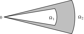
Figure 1.1. Domains $\Omega_{1}\subset\Omega_{2}$

We can also define the asymptotic expansion of a real analytic function: if $K$ is an open interval of the real axis with $0$ as its one of the boundary points and $h(z)$ a real analytic function on $K$, then the same formula (1.3), replacing $\Omega$ by $K$, defines the asymptotic expansion of $h(z)$ at $z=0$.

Now let us compute the asymptotic expansion of $Z(t)$ of (1.2) as a holomorphic function defined on $\Omega_{\epsilon}=\{t\in{\mathbb{C}}|\pi/2+\epsilon<\arg(t)<3\pi/2-\epsilon\}$. The Taylor expansion of the exponential gives

$$\int_{-\infty}^{\infty}e^{-x^{2}/2}e^{t\cdot x^{4}/4!}\frac{dx}{\sqrt{2\pi}}=\int_{-\infty}^{\infty}e^{-x^{2}/2}\sum_{v=0}^{\infty}\frac{1}{(4!)^{v}\cdot v!}\cdot x^{4v}\cdot t^{v}\cdot\frac{dx}{\sqrt{2\pi}}.$$

The infinite integral and the infinite sum we have here are not interchangeable. But let’s just interchange them and see what happens:

(1.5) $$\sum_{v=0}^{\infty}\frac{1}{(4!)^{v}\cdot v!}\left(\int_{-\infty}^{\infty}e^{-x^{2}/2}\cdot x^{4v}\cdot\frac{dx}{\sqrt{2\pi}}\right)t^{v}.$$

Note that this is a well-defined formal power series in $t$ because the integral

$$\int_{-\infty}^{\infty}e^{-x^{2}/2}\cdot x^{4v}\cdot\frac{dx}{\sqrt{2\pi}}$$

converges.

Lemma 1.2.

The formal power series (1.5) gives the asymptotic expansion of $Z(t)$:

$${\mathcal{A}}\left(\int_{-\infty}^{\infty}e^{-x^{2}/2}\sum_{v=0}^{\infty}\frac{1}{(4!)^{v}\cdot v!}\cdot x^{4v}\cdot t^{v}\cdot\frac{dx}{\sqrt{2\pi}}\right)\\ =\sum_{v=0}^{\infty}\frac{t^{v}}{(4!)^{v}\cdot v!}\left(\int_{-\infty}^{\infty}e^{-x^{2}/2}\cdot x^{4v}\cdot\frac{dx}{\sqrt{2\pi}}\right).$$

Although we cannot get an equality by interchanging the integral and the sum because the power series expansion of the integrand of Lemma 1.2 is not uniformly convergent on the infinite interval $(-\infty,\infty)$, at least we obtain a formula which is correct in one direction.

Proof.

Using the linearity of the integral, we have

$$\int_{-\infty}^{\infty}e^{-x^{2}/2}\sum_{v=0}^{\infty}\frac{1}{(4!)^{v}\cdot v!}\cdot x^{4v}\cdot t^{v}\cdot\frac{dx}{\sqrt{2\pi}}-\sum_{v=0}^{m}\frac{t^{v}}{(4!)^{v}\cdot v!}\int_{-\infty}^{\infty}e^{-x^{2}/2}\cdot x^{4v}\cdot\frac{dx}{\sqrt{2\pi}}$$

$$= \int_{-\infty}^{\infty}e^{-x^{2}/2}\sum_{v=m+1}^{\infty}\frac{1}{(4!)^{v}\cdot v!}\cdot x^{4v}\cdot t^{v}\cdot\frac{dx}{\sqrt{2\pi}}$$

$$= t^{m+1}\int_{-\infty}^{\infty}e^{-x^{2}/2}\sum_{a=0}^{\infty}\frac{1}{(4!)^{m+1+a}\cdot{(m+1+a)!}}\cdot x^{4(m+1+a)}\cdot t^{a}\cdot\frac{dx}{\sqrt{2\pi}}.$$

As long as $t$ stays in $\Omega_{\epsilon}=\{t\in{\mathbb{C}}|\pi/2+\epsilon<\arg(t)<3\pi/2-\epsilon\}$, we can divide the above expression by $t^{m+1}$ and take the limit $t\rightarrow 0$, because the integral converges. The result is the $(m+1)$-th coefficient of the asymptotic expansion, which proves the claim. ∎

How can we calculate the coefficient of the expansion? The standard technique is the following:

$$\int_{-\infty}^{\infty}e^{-x^{2}/2}\cdot x^{4v}\cdot\frac{dx}{\sqrt{2\pi}} =\int_{-\infty}^{\infty}e^{-x^{2}/2}\cdot\left.\left(\frac{d}{dy}\right)^{4v}e^{xy}\right|_{y=0}\cdot\frac{dx}{\sqrt{2\pi}}$$

$$=\left(\frac{d}{dy}\right)^{4v}\int_{-\infty}^{\infty}e^{-x^{2}/2}\cdot e^{xy}\cdot\left.\frac{dx}{\sqrt{2\pi}}\right|_{y=0}$$

$$=\left(\frac{d}{dy}\right)^{4v}\left.\int_{-\infty}^{\infty}e^{-(x-y)^{2}/2}\cdot e^{y^{2}/2}\cdot\frac{dx}{\sqrt{2\pi}}\right|_{y=0}$$

$$=\left.\left(\frac{d}{dy}\right)^{4v}e^{y^{2}/2}\right|_{y=0},$$

where we have used the translational invariance of the integral (1.1). Note that the integration is reduced to a differentiation. All we need now is a Taylor coefficient of the exponential function $e^{y^{2}/2}$, from which we obtain

(1.6) $$\int_{-\infty}^{\infty}e^{-x^{2}/2}\cdot x^{4v}\cdot\frac{dx}{\sqrt{2\pi}}=\left.\left(\frac{d}{dy}\right)^{4v}e^{y^{2}/2}\right|_{y=0}=\frac{(4v)!}{(2v)!\cdot 2^{2v}}=(4v-1)!!,$$

where the double factorial is defined by

$$(2n-1)!!=(2n-1)\cdot(2n-3)\cdot(2n-5)\cdots 5\cdot 3\cdot 1.$$

The quantity (1.6) has a combinatorial meaning. Let us denote the differential operator $d/dy$ by a dot $\bullet$. We have $4v$ dots attacking the fort $e^{y^{2}/2}$. Since $y$ is set equal to $0$ after the operation, if only one dot attacks the fort, the result would be just $0$:

$$\left.\frac{d}{dy}\ e^{y^{2}/2}\right|_{y=0}=y\ e^{y^{2}/2}\big{|}_{y=0}=0.$$

To obtain a nonzero result, the dots have to attack the fort by pairs:

$$\left.\left(\frac{d}{dy}\right)^{2}e^{y^{2}/2}\right|_{y=0}=y^{2}\ e^{y^{2}/2}\big{|}_{y=0}+e^{y^{2}/2}\big{|}_{y=0}=1.$$

Noting that the result we get by the paired attack is $1$, we conclude that the value of the integral (or the differentiation) (1.6) is equal to

$${\text{\emph{The number of ways of making $2v$ pairs out of $4v$ dots}}}\\ \begin{aligned} =&\binom{4v}{2}\binom{4v-2}{2}\binom{4v-4}{2}\cdots\left.\binom{4}{2}\binom{2}{2}\right/(2v)!\\ =&\frac{4v(4v-1)}{2}\cdot\frac{(4v-2)(4v-3)}{2}\cdots\frac{4\cdot 3}{2}\cdot\left.\frac{2\cdot 1}{2}\right/(2v)!\\ =&\frac{(4v)!}{(2v)!\cdot 2^{2v}}.\end{aligned}$$

These pairs can be visualized by a diagram like Figure 1.2. Let us call such a diagram a pairing scheme. Thus (1.6) gives the number of pairing schemes of $4v$ dots. An example of a pairing scheme of $8=4\times 2$ dots is given in Figure 1.2.

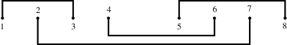
Figure 1.2. Pairing Scheme

The coefficient of the asymptotic expansion of Lemma 1.2 has an extra factor of $1/(4!)^{v}\cdot{v}!$. How can we interpret it combinatorially? Here enters the idea of Feynman diagrams. The $4v$ dots are grouped into $v$ sets of $4$ dots. Let us replace each set of $4$ dots by a cross, identifying the four dots with the four endpoints of the cross. Then the pairing scheme changes into a Feynman diagram, as shown in Figure 1.3, by connecting the endpoints according to the pairing rules. This is an example of a graph. We use this word for a CW complex like Figure 1.3 in this article. A graph $\Gamma=(V,E,i)$ consists of a finite set $V$ of vertices, a finite set $E$ of edges, and the incidence relation $i$ of vertices and edges. The number of half-edges coming out of a vertex of a graph is called the degree of the vertex. A degree $d$ graph is a graph whose vertices have the same degree $d$. A degree $3$ graph is also called a trivalent graph. The order of the graph $\Gamma$ is the number of vertices $|V|$ of $\Gamma$.

When we make the Feynman diagram $\Gamma$ from a pairing scheme, we consider the center of a cross as a vertex and a pairing of dots as an edge of the graph $\Gamma$. Figure 1.3 is thus considered as a degree $4$ graph of order $2$.

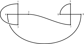
Figure 1.3. Feynman Diagram

As a graph we can interchange the $v$ crosses freely, and in each cross we can place the four edges in any way we want, as long as the strings are attached. The degrees of freedom for these moves are exactly $(4!)^{v}\cdot v!$. Thus we (tentatively) conclude that the $v$-th coefficient of the asymptotic expansion of the integral $Z(t)$ is the number of degree $4$ graphs of order $v$. As an example, let us compute the simplest case $v=1$. From the above considerations, the number of degree $4$ graphs with one vertex should be

$$\frac{(4-1)!!}{4!}=\frac{1}{8}.$$

But this is impossible! What went wrong?

The number of different pairing schemes of $4$ dots is three, as in Figure 1.4. When we factored out (1.6) by $(4!)^{v}\cdot v!$, we assumed that interchanging the $v$ crosses and renumbering each edge of a cross would lead to a different pairing scheme that still corresponds to the same graph. In other words, we assumed that the group ${\mathfrak{S}}_{v}\rtimes({\mathfrak{S}}_{4})^{v}$ acts on the set of all pairing schemes freely, where ${\mathfrak{S}}_{n}$ denotes the permutation group of $n$ letters, and the product is the semi-direct product of two factors with $({\mathfrak{S}}_{4})^{v}$ as its normal subgroup. But as we see clearly from the above example, some pairing schemes are stable under the action of non-trivial permutations. The isotropy group that stabilizes any of the three pairing schemes of Figure 1.4 is $({\mathbb{Z}}\big{/}2{\mathbb{Z}})^{3}$.

Figure 1.4. Pairing Schemes of 4 Dots

Since our graphs are constructed from pairing schemes, we define the automorphism group in the following manner:

Definition 1.3.

The automorphism group ${\text{\rm Aut}}(\Gamma)$ of a graph $\Gamma$ is the isotropy subgroup $I_{P}$ of ${\mathfrak{S}}_{v}{\rtimes}({\mathfrak{S}}_{4})^{v}$ that preserves the original pairing scheme $P$. If pairing schemes $P$ and $P^{\prime}$ correspond to $\Gamma$, then the isotropy groups $I_{P}$ and $I_{P^{\prime}}$ are conjugate to one another in ${\mathfrak{S}}_{v}\rtimes({\mathfrak{S}}_{4})^{v}$. Therefore, as an abstract group, ${\text{\rm Aut}}(\Gamma)$ is well-defined.

Remark.

Our definition of ${\text{\rm Aut}}(\Gamma)$ does not coincide with the traditional graph theoretic definition of automorphism.

The correct interpretation of $1/8$ is then $1/|{\text{\rm Aut}}(\Gamma)|$, where $\Gamma$ in this case is the degree $4$ graph with only one vertex, and we denote by $|{\text{\rm Aut}}(\Gamma)|$ the order of the group. More generally, we can interpret the formal power series (1.5) as a summation over the set of all pairing schemes modulo the group ${\mathfrak{S}}_{v}\rtimes({\mathfrak{S}}_{4})^{v}$, which is equivalent to the set of all degree $4$ graphs. The contribution of a graph $\Gamma$ is modified by the weight of $1/|{\text{\rm Aut}}(\Gamma)|$. Summarizing, we have established: The asymptotic expansion of the integral $Z(t)$ is given by

$${{\mathcal{A}}}\left(\int_{-\infty}^{\infty}e^{-x^{2}/2}e^{t\cdot x^{4}/4!}\frac{dx}{\sqrt{2\pi}}\right)=\sum_{v=0}^{\infty}\left(\sum_{\begin{subarray}{c}{\text{degree $4$ graph}}\\ \Gamma{\text{ of order $v$}}\end{subarray}}\frac{1}{|{\text{\rm Aut}}(\Gamma)|}\right)\cdot t^{v}.$$

Since the number of degree $4$ graphs with a fixed number of vertices is finite, the right hand side of the above formula is a well-defined element of the power series ring ${\mathbb{Q}}[[t]]$. The degree of each vertex of the graph is $4$, which is due to the power $4$ in the exponent of the integral. The same argument thus establishes

Theorem 1.4.

The asymptotic formula

$${{\mathcal{A}}}\left(\int_{-\infty}^{\infty}e^{-x^{2}/2}e^{t\cdot x^{2j}/(2j)!}\frac{dx}{\sqrt{2\pi}}\right)=\sum_{v=0}^{\infty}\left(\sum_{\begin{subarray}{c}{\text{degree $2j$ graph }}\\ \Gamma{\text{ of order $v$}}\end{subarray}}\frac{1}{|{\text{\rm Aut}}(\Gamma)|}\right)\cdot t^{v}\in{\mathbb{Q}}[[t]]$$

holds for an arbitrary $j\geq 2$.

We can consider more general graphs with the integral

(1.7) $$Z(t_{1},t_{2},\cdots,t_{2m})=\int_{-\infty}^{\infty}e^{-x^{2}/2}{{\text{\rm exp}}}\left(\sum_{j=1}^{2m}\frac{t_{j}}{j!}x^{j}\right)\frac{dx}{\sqrt{2\pi}},$$

where $m\geq 2$ is an integer. The integral converges if $t_{2m}$ is in the domain $\Omega_{\epsilon}$ of (1.4) and determines a holomorphic function on

$$(t_{1},t_{2},\cdots,t_{2m})\in{\mathbb{C}}^{2m-1}\times\Omega_{\epsilon}.$$

We can expand $Z(t_{1},t_{2},\cdots,t_{2m})$ as a Taylor series in $(t_{1},t_{2},\cdots,t_{2m-1})\in{\mathbb{C}}^{2m-1}$ and as an asymptotic series in $t_{2m}\in\Omega_{\epsilon}$ at the origin. Fix a value of $t_{2m}\in\Omega_{\epsilon}$. Then

$${{\text{\rm exp}}}\left({t_{2m}}\cdot x^{2m}/{(2m)!}\right)$$

acts as a uniformizing factor so that the power series expansion of the integrand in terms of $x$ converges uniformly on $(-\infty,\infty)$ for all values of $t_{1}$, $t_{2}$, $\cdots$, $t_{2m-1}\in{\mathbb{C}}$. Therefore, we can interchange the infinite integral and the infinite sums:

$$Z(t_{1},t_{2},\cdots,t_{2m})=\int_{-\infty}^{\infty}e^{-x^{2}/2}{{\text{\rm exp}}}\left(\sum_{j=1}^{2m}\frac{t_{j}}{j!}x^{j}\right)\frac{dx}{\sqrt{2\pi}}$$

$$=\int_{-\infty}^{\infty}e^{-x^{2}/2}{{\text{\rm exp}}}\left(\frac{t_{1}}{1!}x\right)\cdots{{\text{\rm exp}}}\left(\frac{t_{2m-1}}{(2m-1)!}x^{2m-1}\right)\cdot{{\text{\rm exp}}}\left(\frac{t_{2m}}{(2m)!}x^{2m}\right)\frac{dx}{\sqrt{2\pi}}$$

$$=\int_{-\infty}^{\infty}e^{-x^{2}/2}\left(\sum_{v_{1}=0}^{\infty}\frac{{t_{1}}^{v_{1}}}{v_{1}!\cdot(1!)^{v_{1}}}\right)\cdots\left(\sum_{v_{2m-1}=0}^{\infty}\frac{{t_{2m-1}}^{v_{2m-1}}}{v_{2m-1}!\cdot((2m-1)!)^{v_{2m-1}}}\right)$$

$$\quad\times\left(\sum_{v_{2m}=0}^{\infty}\frac{{t_{2m}}^{v_{2m}}}{v_{2m}!\cdot((2m)!)^{v_{2m}}}\right)x^{v_{1}+2v_{2}+\cdots+(2m)v_{2m}}\frac{dx}{\sqrt{2\pi}}$$

$$=\left(\sum_{v_{1}=0}^{\infty}\frac{{t_{1}}^{v_{1}}}{v_{1}!\cdot(1!)^{v_{1}}}\right)\cdots\left(\sum_{v_{2m-1}=0}^{\infty}\frac{{t_{2m-1}}^{v_{2m-1}}}{v_{2m-1}!\cdot((2m-1)!)^{v_{2m-1}}}\right)$$

$$\quad\times\int_{-\infty}^{\infty}e^{-x^{2}/2}\left(\sum_{v_{2m}=0}^{\infty}\frac{{t_{2m}}^{v_{2m}}}{v_{2m}!\cdot((2m)!)^{v_{2m}}}\right)x^{v_{1}+2v_{2}+\cdots+(2m)v_{2m}}\frac{dx}{\sqrt{2\pi}}.$$

We already know that

$${\mathcal{A}}\left(\int_{-\infty}^{\infty}e^{-x^{2}/2}\left(\sum_{v_{2m}=0}^{\infty}\frac{{t_{2m}}^{v_{2m}}}{v_{2m}!\cdot((2m)!)^{v_{2m}}}\right)x^{v_{1}+2v_{2}+\cdots+(2m)v_{2m}}\frac{dx}{\sqrt{2\pi}}\right)\\ =\sum_{v_{2m}=0}^{\infty}\frac{{t_{2m}}^{v_{2m}}}{v_{2m}!\cdot((2m)!)^{v_{2m}}}\int_{-\infty}^{\infty}e^{-x^{2}/2}x^{v_{1}+2v_{2}+\cdots+(2m)v_{2m}}\frac{dx}{\sqrt{2\pi}}$$

at $t_{2m}=0$ when the top integral is considered to be a holomorphic function in $t_{2m}\in\Omega_{\epsilon}$ . Therefore, we have

(1.8) $${{\mathcal{A}}}\left(\int_{-\infty}^{\infty}e^{-x^{2}/2}{{\text{\rm exp}}}\left(\sum_{j=1}^{2m}\frac{t_{j}}{j!}x^{j}\right)\frac{dx}{\sqrt{2\pi}}\right)\\ =\sum_{v_{1}=0}^{\infty}\frac{{t_{1}}^{v_{1}}}{v_{1}!\cdot(1!)^{v_{1}}}\cdots\sum_{v_{2m}=0}^{\infty}\frac{{t_{2m}}^{v_{2m}}}{v_{2m}!\cdot((2m)!)^{v_{2m}}}\int_{-\infty}^{\infty}e^{-x^{2}/2}x^{v_{1}+2v_{2}+\cdots+(2m)v_{2m}}\frac{dx}{\sqrt{2\pi}}.$$

We now apply the Feynman diagram expansion to the above integral. First, we have

$$\int_{-\infty}^{\infty}e^{-x^{2}/2}x^{v_{1}+2v_{2}+\cdots+(2m)v_{2m}}\frac{dx}{\sqrt{2\pi}}=\left.\left(\frac{d}{dy}\right)^{v_{1}+2v_{2}+\cdots+(2m)v_{2m}}e^{y^{2}/2}\right|_{y=0}.$$

The pairing scheme of the dot diagram has $v_{1}$ sets of single dot, $v_{2}$ sets of double dots, $\cdots$, and $v_{2m}$ sets of $2m$ dots. Passing to a Feynman diagram, we have a graph with $v_{j}$ vertices of degree $j$ for $j=1,2,\cdots,2m$. Thus

Theorem 1.5.

We have the following asymptotic formula:

$${{\mathcal{A}}}\left(\int_{-\infty}^{\infty}e^{-x^{2}/2}{\text{\rm exp}}\left(\sum_{j=1}^{2m}\frac{t_{j}}{j!}x^{j}\right)\frac{dx}{\sqrt{2\pi}}\right)=\sum_{\begin{subarray}{c}{\text{Graph }}\Gamma{\text{ with}}\\ {\text{vertices of degree }}\leq 2m\end{subarray}}\frac{1}{|{\text{\rm Aut}}(\Gamma)|}\cdot\prod_{j=1}^{2m}t_{j}^{v_{j}(\Gamma)},$$

where $v_{j}(\Gamma)$ denotes the number of vertices of degree $j$ in $\Gamma$.

Note that the asymptotic series is a well-defined element of the formal power series ring

$${\mathbb{Q}}[[t_{1},t_{2},\cdots,t_{2m}]],$$

because there are only finitely many graphs for given numbers $v_{1}(\Gamma)$, $v_{2}(\Gamma)$, $\cdots$, $v_{2m}(\Gamma)$.

Definition 1.6.

The automorphism group of $\Gamma$ is defined as the isotropy subgroup of

$$\prod_{j=1}^{2m}{\mathfrak{S}}_{v_{j}}\rtimes{\mathfrak{S}}_{j}^{v_{j}}$$

that stabilizes the pairing scheme corresponding to $\Gamma$.

As before, the definition of ${\text{\rm Aut}}(\Gamma)$ as an abstract group does not depend on the particular choice of the pairing scheme corresponding to the graph.

Let us now consider the relation between general graphs and connected graphs. Let $a_{v}$ be the number of arbitrary degree $j$ graphs of order $v$ and $c_{v}$ the number of connected degree $j$ graphs of order $v$, where $j\geq 1$ is a fixed number. From Figure 1.5, it is obvious that

(1.9) $$a_{v}=\sum_{n_{1}+2n_{2}+3n_{3}+\cdots=v}\frac{c_{1}^{n_{1}}\cdot c_{2}^{n_{2}}\cdot c_{3}^{n_{3}}\cdots}{n_{1}!\cdot n_{2}!\cdot n_{3}!\cdots},$$

where $n_{i}$ is the number of connected components with $i$ vertices in a given graph. Formula (1.9) is equivalent to a simple functional relation in terms of generating functions:

(1.10) $$\sum_{v=0}^{\infty}a_{v}t_{j}^{v}={\text{\rm exp}}\left(\sum_{v=1}^{\infty}c_{v}t_{j}^{v}\right),$$

where we use the convention that $a_{0}=1$ and $c_{0}=0$.

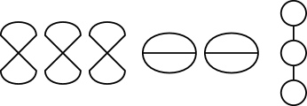
Figure 1.5. A Disconnected Graph

In a more general case, let $\mathbf{v}=(v_{1},v_{2},\cdots,v_{2m})$ and

$$t^{\mathbf{v}}=\prod_{j=1}^{2m}t_{j}^{v_{j}}.$$

We denote by $c_{\mathbf{v}}$ the number of connected graphs with $v_{j}$ vertices of degree $j$, where $1\leq j\leq 2m$, and by $a_{\mathbf{v}}$ the number of all graphs with $v_{j}$ vertices of degree $j$. Then we have

(1.11) $$\begin{split}\sum_{\mathbf{v}}a_{\mathbf{v}}t^{\mathbf{v}}&={\text{\rm exp}}\left(\sum_{\mathbf{v}}c_{\mathbf{v}}t^{\mathbf{v}}\right)\\ &=1+\sum_{\mathbf{v}}c_{\mathbf{v}}t^{\mathbf{v}}+\frac{1}{2!}\left(\sum_{\mathbf{v}}c_{\mathbf{v}}t^{\mathbf{v}}\right)^{2}+\frac{1}{3!}\left(\sum_{\mathbf{v}}c_{\mathbf{v}}t^{\mathbf{v}}\right)^{3}+\cdots,\end{split}$$

where the $n$-th term of the right hand side counts the number of graphs consisting of $n$ connected components. The factor $1/(n!)$ means that we can permute the $n$ connected components without changing the original graph.

The case we are considering is slightly more complicated because the generating function we have in Theorem 1.5 counts the number of graphs with weight $1\big{/}|{\text{\rm Aut}}(\Gamma)|$. The automorphism group of a graph $\Gamma$ consisting of $n$ connected components $\Gamma_{1}$, $\cdots$, $\Gamma_{n}$ is the semi-direct product

(1.12) $${\text{\rm Aut}}(\Gamma)={\mathfrak{S}}_{n}\rtimes\prod_{j=1}^{n}{\text{\rm Aut}}(\Gamma_{j}).$$

Therefore, we have

$$\frac{1}{|{\text{\rm Aut}}(\Gamma)|}=\frac{1}{n!}\cdot\prod_{j=1}^{n}\frac{1}{|{\text{\rm Aut}}(\Gamma_{j})|}.$$

Note that the right hand side is the product of $n$ factors following the key factor $1/(n!)$. It shows, therefore, that the exponential formula (1.11) connecting connected graphs and general graphs also holds in the case we are investigating. Thus we have established

Theorem 1.7.

The asymptotic series involving only connected graphs is given by

$$\log{{\mathcal{A}}}\left(\int_{-\infty}^{\infty}e^{-x^{2}/2}{\text{\rm exp}}\left(\sum_{j=1}^{2m}\frac{t_{j}}{j!}x^{j}\right)\frac{dx}{\sqrt{2\pi}}\right)\\ =\sum_{\begin{subarray}{c}{\text{Connected graph }}\Gamma{\text{ with}}\\ {\text{vertices of degree }}\leq 2m\end{subarray}}\frac{1}{|{\text{\rm Aut}}(\Gamma)|}\cdot\prod_{j=1}^{2m}t_{j}^{v_{j}(\Gamma)}.$$

We note here that the function $\log$ is not considered as an analytic function. It is applied to the formal power series appearing in the right hand side of Theorem 1.5 as the inverse power series of ${\text{\rm exp}}(z)$ defined by

$$\log(1-z)=-\sum_{n=1}^{\infty}\frac{1}{n}z^{n}.$$

2. Matrix integrals and ribbon graphs/fatgraphs

Let ${\mathcal{H}}_{n}$ denote the space of all $n\times n$ Hermitian matrices. It is an $n^{2}$-dimensional Euclidean space with a metric

$$\sqrt{{\text{\rm trace}}(X-Y)^{2}},\qquad X,Y\in{\mathcal{H}}_{n}.$$

The standard volume form on ${\mathcal{H}}_{n}$, which is compatible with the above metric, is given by

$$d\mu(X)=dx_{11}\wedge dx_{22}\wedge\cdots\wedge dx_{nn}\wedge\left(\bigwedge_{i<j}d(Rex_{ij})\wedge d(Imx_{ij})\right)$$

for $X=[x_{ij}]\in{\mathcal{H}}_{n}$. It is important to note that the metric and the volume form of ${\mathcal{H}}_{n}$ are invariant under the conjugation $X\longmapsto UXU^{-1}$ by a unitary matrix $U\in U(n)$. The main subject of this section is the Hermitian matrix integral

(2.1) $$Z_{n}(t,m)=\int_{{\mathcal{H}}_{n}}{\text{\rm exp}}\left(-\frac{1}{2}{\text{\rm trace}}(X^{2})\right){\text{\rm exp}}\left({\text{\rm trace}}\sum_{j=3}^{2m}\frac{t_{j}}{j}X^{j}\right)\frac{d\mu(X)}{N},$$

where

(2.2) $$N=\int_{{\mathcal{H}}_{n}}{\text{\rm exp}}\left(-\frac{1}{2}{\text{\rm trace}}(X^{2})\right)d\mu(X)=2^{n/2}\cdot\pi^{n^{2}/2}$$

is a normalization constant to make $Z_{n}(0,m)=1$. We note that $Z_{n}(t,m)$ is a holomorphic function in $(t_{3},t_{4},\cdots,t_{2m-1})\in{\mathbb{C}}^{2m-3}$ and

$$t_{2m}\in\Omega_{\epsilon}=\{t\in\mathbb{C}|\pi/2+\epsilon<\arg(t)<3\pi/2-\epsilon\}$$

($\epsilon>0$), because the dominating term ${\text{\rm trace}}(X^{2m})$ is positive definite on ${\mathcal{H}}_{n}$. Thus we can expand $Z_{n}(t,m)$ as a convergent power series in $t_{3}$, $t_{4}$, $\cdots$, $t_{2m-1}$ about $0$, and as an asymptotic series in $t_{2m}$ at $t_{2m}=0$.

We also note here that we do not include the $t_{1}$ and $t_{2}$ terms in the integral because of our interests in topology, which will become clearer as we proceed. From the point of view of graphs, we do not allow degree $1$ and $2$ vertices in this section.

Corresponding to the fact that the integral (2.1) has richer structure than (1.8), the Feynman diagrams appearing in the asymptotic expansion of $Z_{n}(t,m)$ have more information than just a graph as in Theorem 1.5. As we are going to see below, the new information we have from the Hermitian matrix integral is that the graph is drawn on a compact oriented surface. Suppose we have such a graph drawn on an oriented surface, as in Figure 2.1.

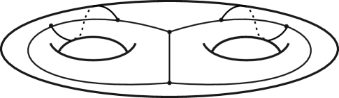
Figure 2.1. Graph on a Surface

Locally at each vertex of the graph, the orientation of the surface gives rise to a cyclic order of the edges coming out of the vertex, as shown in Figure 2.2.

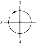
Figure 2.2. Cyclic Order of Edges

A graph drawn on a surface thus gives a graph with a cyclic order of edges at each vertex. An example, that is corresponding to Figure 2.1, is shown in Figure 2.3.

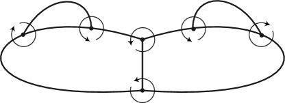
Figure 2.3. Ribbon Graph

Note that two circles are reversed in Figure 2.3, corresponding to the fact that two edges of the graph of Figure 2.1 go around the back side of the surface.

Conversely, suppose we have a connected graph $\Gamma_{rib}$ with a cyclic order of edges assigned to each vertex. To indicate that we have the extra information of cyclic order at each vertex, we use $\Gamma_{rib}$ and distinguish it from the underlying graph $\Gamma$. We can construct a compact oriented surface $C(\Gamma_{rib})$ canonically such that the graph $\Gamma$ is drawn on it, as follows. First, the graph around each vertex can be drawn on a positively oriented plane that is compatible with the cyclic order. Next we fatten the local part of the graph into a crossroad of multiple intersection. The orientation of the plane defines an orientation on each sidewalk of the crossroad, as in Figure 2.4.

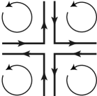
Figure 2.4. Oriented Crossroad

The roads are connected to the other parts of the graph, with matching orientation on the sidewalks. Then we obtain an oriented surface with boundary. Figure 2.5 shows such a surface with boundary.

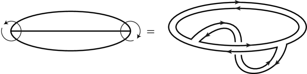
Figure 2.5. Ribbon Graph and Surface with Boundary

Let $b(\Gamma_{rib})$ denote the number of boundary components of this oriented surface ($=$ fattened graph) made out of $\Gamma_{rib}$. From the construction, each boundary component has a unique orientation compatible with that of the fattened graph. Thus a boundary component is indeed an oriented circle, which we also call a boundary circuit. So we can attach an oriented $2$-dimensional disk to each boundary component of the fattened graph to construct a compact oriented surface $C(\Gamma_{rib})$.

Definition 2.1.

A ribbon graph (or a fatgraph) is a graph with a cyclic order of edges assigned to each vertex.

The ribbon graph $\Gamma_{rib}$ of Figure 2.5 has only one boundary component, and the resulting compact surface $C(\Gamma_{rib})$ is the 2-torus on which the underlying graph $\Gamma$ is drawn (Figure 2.6).

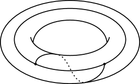
Figure 2.6. 3-valent Graph on a Torus

We have shown that every graph drawn on an oriented surface is a ribbon graph, and conversely, that every connected ribbon graph $\Gamma_{rib}$ gives rise to a canonical compact oriented surface $C(\Gamma_{rib})$ on which the underlying graph is drawn. The attached boundary disks and the underlying graph $\Gamma$ give a cell-decomposition of $C(\Gamma_{rib})$.

Lemma 2.2.

Let $\Gamma_{rib}$ be a connected ribbon graph with vertices of degree $\geq 3$, and $v_{j}(\Gamma)$ denote the number of vertices of the underlying graph $\Gamma$ of degree $j$. Then the genus $g(C(\Gamma_{rib}))$ of the canonical oriented surface $C(\Gamma_{rib})$ associated with $\Gamma_{rib}$ is computed by the following formula:

$$2-2g(C(\Gamma_{rib}))=\sum_{j\geq 3}v_{j}(\Gamma)-\frac{1}{2}\sum_{j\geq 3}j\cdot v_{j}(\Gamma)+s(\Gamma_{rib}).$$

Proof.

The total number of vertices of the cell-decomposition is given by $\sum_{j\geq 3}v_{j}(\Gamma)$. Since each edge is bounded by two vertices (possibly the same), the number of edges is given by $\frac{1}{2}\sum_{j\geq 3}j\cdot v_{j}(\Gamma)$. By construction, $b(\Gamma_{rib})$ is the number of $2$-cells. Thus the Euler characteristic of a compact surface gives the above formula. ∎

To see how ribbon graphs appear in the matrix integral, let us consider a simple example:

$$\int_{{\mathcal{H}}_{n}}{\text{\rm exp}}\left(-\frac{1}{2}{\text{\rm trace}}(X^{2})\right)\cdot{\text{\rm exp}}\left(\frac{t}{4}{\text{\rm trace}}X^{4}\right)\frac{d\mu(X)}{N}.$$

Using the same argument as in Lemma 1.2 we can prove the asymptotic formula

$${{\mathcal{A}}}\left(\int_{{\mathcal{H}}_{n}}{\text{\rm exp}}\left(-\frac{1}{2}{\text{\rm trace}}(X^{2})\right)\cdot{\text{\rm exp}}\left(\frac{t}{4}{\text{\rm trace}}X^{4}\right)\frac{d\mu(X)}{N}\right)\\ =\sum_{v=0}^{\infty}\frac{t^{v}}{4!\cdot v!}\int_{{\mathcal{H}}_{n}}{\text{\rm exp}}\left(-\frac{1}{2}{\text{\rm trace}}(X^{2})\right)\cdot\big{(}{\text{\rm trace}}X^{4}\big{)}^{v}\frac{d\mu(X)}{N}.$$

We need another matrix $Y=[y_{ij}]\in{\mathcal{H}}_{n}$ and a differential operator

$$\frac{\partial}{\partial Y}=\left[\frac{\partial}{\partial y_{ij}}\right]$$

to compute the asymptotic expansion of the integral.

Lemma 2.3.

For every $j>0$ and $v>0$, we have

(2.3) $$\left.\left({\text{\rm trace}}\left(\frac{\partial}{\partial Y}\right)^{j}\right)^{v}e^{{\text{\rm trace}}(X^{t}\cdot Y)}\right|_{Y=0}=\left({\text{\rm trace}}X^{j}\right)^{v}.$$

Proof.

Suppose that $Y$ and $X$ are both arbitrary complex matrices of size $n$. Then for each $j>0$, we have

$${\text{\rm trace}}\left.\left(\frac{\partial}{\partial Y}\right)^{j}e^{{\text{\rm trace}}(X^{t}\cdot Y)}\right|_{Y=0}\\ =\left.\sum_{i_{1},i_{2},i_{3},\cdots,i_{j}=1}^{n}\frac{\partial}{\partial y_{i_{1}i_{2}}}\frac{\partial}{\partial y_{i_{2}i_{3}}}\cdots\frac{\partial}{\partial y_{i_{j}i_{1}}}{\text{\rm exp}}\left(\sum_{k,\ell=1}^{n}x_{k\ell}\cdot y_{k\ell}\right)\right|_{Y=0}\\ =\sum_{i_{1},i_{2},i_{3},\cdots,i_{j}=1}^{n}x_{i_{1}i_{2}}x_{i_{2}i_{3}}\cdots x_{i_{j}i_{1}}={\text{\rm trace}}X^{j}.$$

Repeating it $v$ times, we obtain the desired formula (2.3) for general complex matrices. Certainly, the formula holds after changing coordinates:

(2.4) $$\begin{cases}y_{ij}=u_{ij}+\sqrt{-1}w_{ij}\quad{\text{ for }}i<j\\ y_{ji}=u_{ij}-\sqrt{-1}w_{ij}\quad{\text{ for }}i<j\\ y_{ii}=u_{ii}\end{cases},$$

where $u_{ij}$ and $w_{ij}$ are complex variables. Since (2.3) is an algebraic formula, it holds for an arbitrary field of characteristic $0$. In particular, (2.3) holds for real $u_{ij}$ and $w_{ij}$, which proves the lemma. ∎

Therefore, we have

$$\int_{{\mathcal{H}}_{n}}{\text{\rm exp}}\left(-\frac{1}{2}{\text{\rm trace}}(X^{2})\right)\cdot\big{(}{\text{\rm trace}}X^{4}\big{)}^{v}\frac{d\mu(X)}{N}$$

$$= \left.\int_{{\mathcal{H}}_{n}}{\text{\rm exp}}\left(-\frac{1}{2}{\text{\rm trace}}(X^{2})\right)\cdot\left({\text{\rm trace}}\left(\frac{\partial}{\partial Y}\right)^{4}\right)^{v}e^{{\text{\rm trace}}(X^{t}\cdot Y)}\right|_{Y=0}\frac{d\mu(X)}{N}$$

$$= \left.\left({\text{\rm trace}}\left(\frac{\partial}{\partial Y}\right)^{4}\right)^{v}\int_{{\mathcal{H}}_{n}}{\text{\rm exp}}\left(-\frac{1}{2}{\text{\rm trace}}(X-Y^{t})^{2}\right)\cdot e^{1/2{\text{\rm trace}}(Y^{t})^{2}}\right|_{Y=0}\frac{d\mu(X)}{N}$$

$$= \left.\left({\text{\rm trace}}\left(\frac{\partial}{\partial Y}\right)^{4}\right)^{v}e^{1/2{\text{\rm trace}}Y^{2}}\right|_{Y=0}$$

$$= \left.\left(\sum_{i,j,k,\ell}\frac{\partial}{\partial y_{ij}}\frac{\partial}{\partial y_{jk}}\frac{\partial}{\partial y_{k\ell}}\frac{\partial}{\partial y_{\ell i}}\right)^{v}{\text{\rm exp}}\left(\frac{1}{2}\sum_{i,j}y_{ij}y_{ji}\right)\right|_{Y=0}.$$

The only nontrivial contribution of the differentiation comes from paired derivatives:

$$\left.\frac{\partial}{\partial y_{ij}}\frac{\partial}{\partial y_{k\ell}}{\text{\rm exp}}\left(\frac{1}{2}\sum_{i,j}y_{ij}y_{ji}\right)\right|_{Y=0}=\frac{\partial}{\partial y_{ij}}y_{\ell k}=\delta_{i\ell}\cdot\delta_{jk}.$$

If we denote by $\bullet_{ij}$ the differential operator $\frac{\partial}{\partial y_{ij}}$, then we have a pairing scheme of $4v$ dots as before, and the pairing of two dots $\bullet_{ij}$ and $\bullet_{k\ell}$ contributes $\delta_{i\ell}\cdot\delta_{jk}$. Thus

(2.5) $$\begin{split}&\left.\left({\text{\rm trace}}\left(\frac{\partial}{\partial Y}\right)^{4}\right)^{v}e^{1/2{\text{\rm trace}}Y^{2}}\right|_{Y=0}\\ &\quad=\sum_{i_{1},j_{1},k_{1},\ell_{1}=1}^{n}\cdots\sum_{i_{v},j_{v},k_{v},\ell_{v}=1}^{n}\sum_{\begin{subarray}{c}{\text{All pairings}}\\ {\text{$P$ of $4v$ dots}}\end{subarray}}\left(\prod_{\begin{subarray}{c}{\text{All paired dots}}\\ (\bullet_{ij},\bullet_{k\ell}){\text{ in }}P\end{subarray}}\delta_{i\ell}\cdot\delta_{jk}\right).\end{split}$$

A symbolic description of the contribution of parings is given in Figures 2.7.

$$\raisebox{-8.53581pt}{\psfig{width=86.72377pt}}=\delta_{ik}\delta_{jj}\delta_{ki}\delta_{\ell\ell}\\ \raisebox{-11.38109pt}{\psfig{width=86.72377pt}}=\delta_{i\ell}\delta_{jk}\delta_{ji}\delta_{k\ell}\\ \raisebox{-11.38109pt}{\psfig{width=86.72377pt}}=\delta_{ii}\delta_{j\ell}\delta_{j\ell}\delta_{kk}$$

Figure 2.7. Pairing Contribution

An interpretation of Figure 2.7 in terms of Feynman Diagrams was introduced by ’tHooft [14]. The set of four indexed dots $\bullet_{ij}\bullet_{jk}\bullet_{k\ell}\bullet_{\ell i}$ is replaced by a crossroad (Figure 2.8).

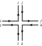
Figure 2.8. Indexed Crossroad

Since $\bullet_{ij}=\frac{\partial}{\partial y_{ij}}$ is different from $\bullet_{ji}=\frac{\partial}{\partial y_{ji}}$, the different roles of the indices are represented by an arrow. If $\bullet_{ij}$ is connected to $\bullet_{jk}$, then it gives a contribution of $\delta_{ik}\cdot\delta_{jj}$. ’tHooft visualized this situation graphically by making a crossroad loop (Figure 2.9).

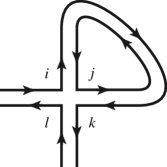
Figure 2.9. Crossroad Loop

Note that the orientation of the sidewalks of this crossroad loop is consistent. Thus we obtain a ribbon graph, as we expected.

The passage from the pairing scheme to a ribbon graph has again some redundancy. In Section 1, the permutation group ${\mathfrak{S}}_{j}$ appeared for a vertex of degree $j$. This is due to the fact that a scalar monomial $x_{1}x_{2}\cdots x_{j}$ is invariant under the ${\mathfrak{S}}_{j}$-action. In the case of matrix integrals, a monomial is of type ${\text{\rm trace}}(X_{1}X_{2}\cdots X_{j})$, which is invariant under the action of the cyclic group ${\mathbb{Z}}/j{\mathbb{Z}}$, but not under the full symmetric group ${\mathfrak{S}}_{j}$. This is the origin of the appearance of the extra cyclic order of the edges at each vertex.

Definition 2.4.

Let $P$ be a pairing scheme of indexed dots and $\Gamma_{rib}$ the corresponding ribbon graph. Then the group

$$\prod_{j}\left({\mathfrak{S}}_{v_{j}(\Gamma)}\rtimes\big{(}{\mathbb{Z}}/j{\mathbb{Z}}\big{)}^{v_{j}(\Gamma)}\right)$$

acts on the set of all pairing schemes. As before, we define the automorphism group of a ribbon graph $\Gamma_{rib}$ to be the isotropy subgroup of the above group that fixes $P$. As an abstract group, ${\text{\rm Aut}}(\Gamma_{rib})$ does not depend on the choice of the pairing scheme of indexed dots corresponding to $\Gamma_{rib}$.

One more difference between the matrix integral and the integrals considered in Section 1 is the appearance of the size of matrix in the calculation. To illustrate this effect, let us continue our consideration of the degree $4$ case with one vertex:

(2.6) $$\begin{split}{}&\frac{1}{4\cdot 1!}\int_{{\mathcal{H}}_{n}}e^{-1/2{\text{\rm trace}}(X^{2})}{\text{\rm trace}}(X^{4})\frac{d\mu(X)}{N}\\ &=\frac{1}{4}\sum_{i,j,k,\ell=1}^{n}\left(\delta_{ik}\delta_{jj}\delta_{ki}\delta_{\ell\ell}+\delta_{i\ell}\delta_{jk}\delta_{ji}\delta_{k\ell}+\delta_{ii}\delta_{j\ell}\delta_{j\ell}\delta_{kk}\right)\\ &=\frac{1}{4}(n^{3}+n+n^{3})=\frac{1}{2}n^{3}+\frac{1}{4}n.\end{split}$$

As shown in Figure 2.10 there are two degree $4$ ribbon graphs of order one. The one on the left has the automorphism group ${\mathbb{Z}}/2{\mathbb{Z}}$, while the second has ${\mathbb{Z}}/4{\mathbb{Z}}$.

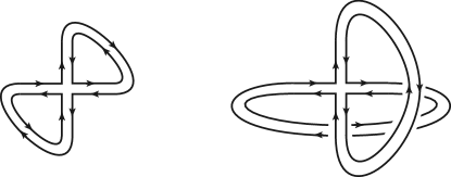
Figure 2.10. Degree 4 Ribbon Graphs with 1 Vertex

We also note that the exponent of $n$ in (LABEL:eq2.45) is exactly the number of boundary components of the ribbon graph which is considered as a surface with boundary. For every $v\geq 1$, we now have

$$\frac{1}{4^{v}\cdot v!}\int_{{\mathcal{H}}_{n}}e^{-1/2{\text{\rm trace}}(X^{2})}\big{(}{\text{\rm trace}}(X^{4})\big{)}^{v}\frac{d\mu(X)}{N}\\ =\sum_{\begin{subarray}{c}{\text{degree $4$ ribbon graph}}\\ \Gamma_{rib}{\text{ of order $v$}}\end{subarray}}\frac{1}{|{\text{\rm Aut}}(\Gamma_{rib})|}n^{b(\Gamma_{rib})}\in{\mathbb{Q}}[n].$$

The same argument that we used to prove Theorem 1.5 works and we have:

Theorem 2.5.

The asymptotic expansion of the Hermitian matrix integral (2.1) is given by

$${{\mathcal{A}}}\left(\int_{{\mathcal{H}}_{n}}{\text{\rm exp}}\left(-\frac{1}{2}{\text{\rm trace}}(X^{2})\right){\text{\rm exp}}\left({\text{\rm trace}}\sum_{j=3}^{2m}\frac{t_{j}}{j}X^{j}\right)\frac{d\mu(X)}{N}\right)\\ =\sum_{\begin{subarray}{c}{\text{Ribbon graph $\Gamma_{rib}$ with}}\\ {\text{vertices of degree }}3,4,\cdots,2m\end{subarray}}\frac{1}{|{\text{\rm Aut}}(\Gamma_{rib})|}n^{b(\Gamma_{rib})}\cdot\prod_{j=3}^{2m}{t_{j}}^{v_{j}(\Gamma)},$$

where $b(\Gamma_{rib})$ denotes the number of boundary components of the ribbon graph $\Gamma_{rib}$, and $v_{j}(\Gamma)$ the number of degree $j$ vertices in the underlying graph $\Gamma$.

Here we note that for given values of $v_{3}(\Gamma),\cdots,v_{2m}(\Gamma)$, the number of ribbon graphs is finite. Thus the above asymptotic series belongs to $\big{(}{\mathbb{Q}}[n]\big{)}[[t_{3},t_{4},\cdots,t_{2m}]]$. The relation between connected ribbon graphs and arbitrary ribbon graphs are the same as in Section 1. In particular, since (1.12) also holds for ribbon graphs, application of the logarithm gives us

Theorem 2.6.

$$\log{{\mathcal{A}}}\left(\int_{{\mathcal{H}}_{n}}{\text{\rm exp}}\left(-\frac{1}{2}{\text{\rm trace}}(X^{2})\right){\text{\rm exp}}\left({\text{\rm trace}}\sum_{j=3}^{2m}\frac{t_{j}}{j}X^{j}\right)\frac{d\mu(X)}{N}\right)\\ =\sum_{\begin{subarray}{c}{\text{Connected ribbon graph $\Gamma_{rib}$}}\\ {\text{with maximum degree }}2m\end{subarray}}\frac{1}{|{\text{\rm Aut}}(\Gamma_{rib})|}n^{b(\Gamma_{rib})}\cdot\prod_{j=3}^{2m}{t_{j}}^{v_{j}(\Gamma)}.$$

This formula is particularly useful, because we are interested in connected Riemann surfaces and only connected ribbon graphs give rise to connected surfaces. Using Lemma 2.2, we can rearrange the summation in terms of the genus of a compact oriented surface and the number of marked points on it:

(2.7) $$\begin{split}&\log{\mathcal{A}}\left(Z_{n}(t,m)\right)\\ &\qquad=\sum_{\begin{subarray}{c}g\geq 0,s>0\\ 2-2g-s<0\end{subarray}}\left(\sum_{\begin{subarray}{c}{\text{Connected ribbon graph }}\Gamma_{rib}\\ {\text{with vertices of degree }}3,4,\cdots,2m,\\ {\hbox{\raise 1.5pt\hbox{$\chi$}}}(\Gamma)=2-2g-s,b(\Gamma_{rib})=s\end{subarray}}\frac{n^{s}}{|{\text{\rm Aut}}(\Gamma_{rib})|}\cdot\prod_{j=3}^{2m}t_{j}^{v_{j}(\Gamma)}\right),\end{split}$$

where ${\hbox{\raise 1.5pt\hbox{$\chi$}}}(\Gamma)$ denotes the Euler characteristic of the underlying graph $\Gamma$. Note that Lemma 2.2 implies that

$$2-2g(C(\Gamma_{rib}))-b(\Gamma_{rib})<0$$

for every ribbon graph $\Gamma_{rib}$. Let $v(\Gamma)$ and $e(\Gamma)$ be the total number of vertices and edges of the graph $\Gamma$, respectively. Then

(2.8) $$\begin{cases}{\hbox{\raise 1.5pt\hbox{$\chi$}}}(\Gamma)=v(\Gamma)-e(\Gamma)\\ v(\Gamma)=v_{3}(\Gamma)+v_{4}(\Gamma)+\cdots+v_{2m}(\Gamma)\\ e(\Gamma)=\frac{1}{2}\big{(}3\cdot v_{3}(\Gamma)+4\cdot v_{4}(\Gamma)+\cdots+2m\cdot v_{2m}(\Gamma)\big{)},\end{cases}$$

because the vertices of $\Gamma$ have degree in between $3$ and $2m$. Thus for every fixed $g$ and $s$, the second summation of (2.7) is a finite sum, which again shows that (2.7) is an element of the formal power series ring

$$\big{(}{\mathbb{Q}}[n]\big{)}[[t_{3},t_{4},\cdots,t_{2m}]].$$

The number $g$ is of course the genus of $C(\Gamma_{rib})$. The topological type of the ribbon graph $\Gamma_{rib}$ is the same as the compact surface $C(\Gamma_{rib})$ minus $b(\Gamma_{rib})$ points. The number of boundary components becomes the number of marked points of a Riemann surface in later sections.

Let $\big{(}{\mathbb{Q}}[n]\big{)}[[t_{3},t_{4},\cdots]]$ be the formal power series ring in infinitely many variables. The adic topology of this ring is given by the degree

$$\deg t_{j}=j,\qquad j\geq 3$$

and the ideal ${\mathfrak{I}}_{j}(t)$ of $\big{(}{\mathbb{Q}}[n]\big{)}[[t_{3},t_{4},\cdots]]$ generated by polynomials in $t_{3},t_{4},\cdots$ of degree greater than $j$, with coefficients in ${\mathbb{Q}}[n]$. We have a natural projection

$$\pi_{j}:\big{(}{\mathbb{Q}}[n]\big{)}[[t_{3},t_{4},\cdots]]\longrightarrow\big{(}{\mathbb{Q}}[n]\big{)}[[t_{3},t_{4},\cdots]]\big{/}{\mathfrak{I}}_{j}(t)=\big{(}{\mathbb{Q}}[n]\big{)}[[t_{3},\cdots,t_{j}]]\big{/}{\mathfrak{I}}_{j}(t).$$

For each fixed $j$, the projection image

$$\pi_{j}\big{(}\log{{\mathcal{A}}}\big{(}Z_{n}(t,m)\big{)}\big{)}\in\big{(}{\mathbb{Q}}[n]\big{)}[[t_{3},t_{4},\cdots]]\big{/}{\mathfrak{I}}_{j}(t)=\big{(}{\mathbb{Q}}[n]\big{)}[[t_{3},\cdots,t_{j}]]\big{/}{\mathfrak{I}}_{j}(t)$$

is stable for all $2m\geq j$. Since

$$\big{(}{\mathbb{Q}}[n]\big{)}[[t_{3},t_{4},\cdots]]=\lim_{\begin{subarray}{c}\longleftarrow\\ j\end{subarray}}\big{(}{\mathbb{Q}}[n]\big{)}[[t_{3},t_{4},\cdots]]\big{/}{\mathfrak{I}}_{j}(t)$$

and

$$\left\{\pi_{2m}\big{(}\log{{\mathcal{A}}}\big{(}Z_{n}(t,m)\big{)}\big{)}\right\}_{m\geq 2}$$

defines an element of the projective system, it gives a well-defined formal power series in infinitely many variables. We denote it symbolically by

(2.9) $$\begin{split}\lim_{m\rightarrow\infty}\log&{{\mathcal{A}}}\big{(}Z_{n}(t,m)\big{)}\\ &\qquad=\left\{\pi_{2m}\big{(}\log{{\mathcal{A}}}\big{(}Z_{n}(t,m)\big{)}\big{)}\right\}_{m\geq 2}\in\big{(}{\mathbb{Q}}[n]\big{)}[[t_{3},t_{4},\cdots]].\end{split}$$

Going back to the Feynman diagram expansion (2.7), we have an equality

(2.10) $$\begin{split}\lim_{m\rightarrow\infty}\log&{{\mathcal{A}}}\big{(}Z_{n}(t,m)\big{)}\\ &\qquad=\sum_{\begin{subarray}{c}g\geq 0,s>0\\ 2-2g-s<0\end{subarray}}\left(\sum_{\begin{subarray}{c}{\text{Connected ribbon graph }}\Gamma_{rib}\\ {\text{with vertices of degree }}\geq 3,\\ {\hbox{\raise 1.5pt\hbox{$\chi$}}}(\Gamma)=2-2g-s,b(\Gamma_{rib})=s\end{subarray}}\frac{n^{s}}{|{\text{\rm Aut}}(\Gamma_{rib})|}\cdot\prod_{j\geq 3}t_{j}^{v_{j}(\Gamma)}\right)\end{split}$$

as an element of $\big{(}{\mathbb{Q}}[n]\big{)}[[t_{3},t_{4},\cdots]]$. For each fixed $g$ and $s$, the maximum possible valency of the ribbon graphs in the second summation is $4g+2s-2$. To see this, let $\Gamma$ be a graph with the largest possible degree $\ell$. Since the Euler characteristic of $\Gamma$ is given by $2-2g-s=v(\Gamma)-e(\Gamma)$, the degree becomes maximum when $\Gamma$ has only one vertex. Thus

$$2-2g-s=1-\frac{1}{2}\ell.$$

This shows us that the right hand side of (2.10) does not have any infinite products.

3. Asymptotic analysis of the Penner model

There are no known analytic methods to compute the matrix integral $Z_{n}(t,m)$ for general $m$. It is therefore an amazing observation of Penner that at the limit of $m\rightarrow\infty$ a certain specialization of $Z_{n}(t,m)$ is actually computable. In this section we study the Penner model and calculate its asymptotic expansion analytically.

The specialization Penner considered is the substitution

(3.1) $$t_{j}=-\big{(}\sqrt{z}\big{)}^{j-2},\quad j=3,4,\cdots,2m$$

in the matrix integral $Z_{n}(t,m)$, where $\sqrt{z}$ is defined for $Re(z)>0$. The condition

$$\pi/2+\epsilon<\arg(t_{2m})<3\pi/2-\epsilon$$

for $t_{2m}$ translates into the condition

(3.2) $$|\arg(z)|<\frac{\pi}{2m-2}.$$

Thus we have a holomorphic function

(3.3) $$\begin{split}&P_{n}(z,m)\\ &=\int_{{\mathcal{H}}_{n}}{\text{\rm exp}}\left(-\frac{1}{2}{\text{\rm trace}}(X^{2})\right){\text{\rm exp}}\left(-\sum_{j=3}^{2m}\frac{(\sqrt{z})^{j-2}}{j}{\text{\rm trace}}(X^{j})\right)\frac{d\mu(X)}{N}\\ &=\int_{{\mathcal{H}}_{n}}{\text{\rm exp}}\left(-\sum_{j=2}^{2m}\frac{(\sqrt{z})^{j-2}}{j}{\text{\rm trace}}(X^{j})\right)\frac{d\mu(X)}{N}\end{split}$$

defined on the region of the complex plane given by (3.2).

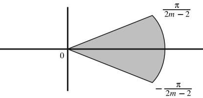
Figure 3.1. Wedge-shape Domain

We note that the domain (3.2) still makes sense as the positive real axis when we take the limit $m\rightarrow\infty$. The quantity $N$ is the same normalization constant as in (2.2).

The asymptotic expansion of (3.3) at $z=0$ can be calculated by making the same substitution (3.1) in Theorem 2.5. Taking the logarithm, we obtain

(3.4) $$\begin{split}\log{\mathcal{A}}&\left(P_{n}(z,m)\right)\\ &=\sum_{\begin{subarray}{c}g\geq 0,s>0\\ 2-2g-s<0\end{subarray}}\left(\sum_{\begin{subarray}{c}{\text{Connected ribbon graph }}\Gamma_{rib}\\ {\text{with vertices of degree }}3,4,\cdots,2m,\\ {\hbox{\raise 1.5pt\hbox{$\chi$}}}(\Gamma)=2-2g-s,b(\Gamma_{rib})=s\end{subarray}}\frac{(-1)^{e(\Gamma)}}{|{\text{\rm Aut}}(\Gamma_{rib})|}\right)n^{s}\cdot(-z)^{2g+s-2},\end{split}$$

where we used (2.8) to compute

$$\prod_{j=3}^{2m}\left(-(\sqrt{z})^{j-2}\right)^{v_{j}(\Gamma)} =(-1)^{\Sigma_{j=3}^{2m}v_{j}(\Gamma)}\cdot z^{\frac{1}{2}\Sigma_{j=3}^{2m}jv_{j}(\Gamma)-\Sigma_{j=3}^{2m}v_{j}(\Gamma)}$$

$$=(-1)^{v(\Gamma)}z^{e(\Gamma)-v(\Gamma)}$$

$$=(-1)^{e(\Gamma)}(-z)^{-{\hbox{\raise 1.5pt\hbox{$\chi$}}}(\Gamma)}.$$

Note that the right hand side of (3.4) is a well-defined element of $\big{(}{\mathbb{Q}}[n]\big{)}[[z]]$. For every $\nu>0$, the terms in $\log{\mathcal{A}}\left(P_{n}(z,m)\right)$ of degree less than or equal to $\nu$ with respect to $z$ are stable for all $m\geq\nu+1$. Again by the same argument we used in Section 2, we can define an element

$$\lim_{m\rightarrow\infty}\log{\mathcal{A}}\left(P_{n}(z,m)\right)\in\big{(}{\mathbb{Q}}[n]\big{)}[[z]].$$

Thus we have an equality

(3.5) $$\begin{split}\lim_{m\rightarrow\infty}\log{{\mathcal{A}}}&\left(\int_{{\mathcal{H}}_{n}}{\text{\rm exp}}\left(-\sum_{j=2}^{2m}\frac{(\sqrt{z})^{j-2}}{j}{\text{\rm trace}}(X^{j})\right)\frac{d\mu(X)}{N}\right)\\ &=\sum_{\begin{subarray}{c}g\geq 0,s>0\\ 2-2g-s<0\end{subarray}}\left(\sum_{\begin{subarray}{c}{\text{Connected ribbon graph }}\Gamma_{r}\\ {\text{ with vertices of degree }}\geq 3,\\ {\hbox{\raise 1.5pt\hbox{$\chi$}}}(\Gamma)=2-2g-s,b(\Gamma_{rib})=s\end{subarray}}\frac{(-1)^{e(\Gamma)}}{|{\text{\rm Aut}}(\Gamma_{rib})|}\right)n^{s}\cdot(-z)^{2g+s-2}\end{split}$$

as a well-defined element of $\big{(}{\mathbb{Q}}[n]\big{)}[[z]]$. We recall that in (2.10) we proved that the number of ribbon graphs in the second summation for fixed $g$ and $s$ is finite.

Let us now compute $\lim_{m\rightarrow\infty}\log{\mathcal{A}}\left(P_{n}(z,m)\right)$. The standard analytic technique to compute the Hermitian matrix integrals is the following formula. Let $f(X)$ be a function on $X\in{\mathcal{H}}_{n}$ which is invariant under the conjugation by a unitary matrix $U\in U(n)$:

$$f(X)=f(U^{-1}\cdot X\cdot U)=f(k_{0},k_{1},\cdots,k_{n-1}),$$

where $k_{0},k_{1},\cdots,k_{n-1}$ are the eigenvalues of the Hermitian matrix $X$. If $f(X)$ is integrable on ${\mathcal{H}}_{n}$ with respect to the measure $d\mu(X)$, then

(3.6) $$\int_{{\mathcal{H}}_{n}}f(X)d\mu(X)=c(n)\cdot\int_{{\mathbb{R}}^{n}}f(k_{0},k_{1},\cdots,k_{n-1})\Delta(k)^{2}dk_{0}dk_{1}\cdots dk_{n-1},$$

where

(3.7) $$c(n)=\frac{\pi^{n(n-1)/2}}{n!\cdot(n-1)!\cdots 2!\cdot 1!},$$

and

$$\Delta(k)=\Delta\big{(}k_{0},k_{1}\cdots,k_{n-1}\big{)}=\det\begin{pmatrix}1&k_{0}&k_{0}^{2}&\ldots&k_{0}^{n-1}\\ 1&k_{1}&k_{1}^{2}&\ldots&k_{1}^{n-1}\\ 1&k_{2}&k_{2}^{2}&\ldots&k_{2}^{n-1}\\ \vdots&\vdots&\vdots&\ddots&\vdots\\ 1&k_{n-1}&k_{n-1}^{2}&\ldots&k_{n-1}^{n-1}\end{pmatrix}=\prod_{i>j}(k_{i}-k_{j})$$

is the Vandermonde determinant. The proof of (3.6) goes as follows:

Let $\overset{\circ}{{\mathcal{H}}}_{n}$ denote the open dense subset of ${\mathcal{H}}_{n}$ consisting of non-singular Hermitian matrices of size $n$ with $n$ distinct eigenvalues. If $f(X)$ is a regular integrable function on ${\mathcal{H}}_{n}$, then

$$\int_{{\mathcal{H}}_{n}}f(X)d\mu(X)=\int_{\overset{\circ}{{\mathcal{H}}}_{n}}f(X)d\mu(X).$$

We denote by $\overset{\circ}{\mathbb{R}}{}^{n}$ the space of real diagonal matrices of all distinct, non-zero eigenvalues. Here again integration over ${\mathbb{R}}^{n}$ is equal to integration over $\overset{\circ}{{\mathbb{R}}}{}^{n}$. Since every Hermitian matrix is diagonalizable by a unitary matrix, we have a surjective map

$$U(n)\times\overset{\circ}{{\mathbb{R}}}{}^{n}\owns\left(U,\begin{bmatrix}k_{0}\\ &\ddots\\ &&k_{n-1}\end{bmatrix}\right)\longmapsto U\cdot\begin{bmatrix}k_{0}\\ &\ddots\\ &&k_{n-1}\end{bmatrix}\cdot U^{-1}\in\overset{\circ}{{\mathcal{H}}}_{n}.$$

The fiber of this map is the set of all unitary matrices that are commutative with a generic real diagonal matrix, which can be identified with the product of two subgroups

$$T^{n}\cdot W_{n}\subset U(n),$$

where $T^{n}\subset U(n)$ is the maximal torus of $U(n)$, and $W_{n}\subset U(n)$ the group of permutation matrices of size $n$. Note that

$$\dim U(n)=\dim{{\mathcal{H}}}_{n}=n^{2},\quad\dim T^{n}=n.$$

Therefore, the induced map

$$h:U(n)\big{/}T^{n}\times\overset{\circ}{{\mathbb{R}}}{}^{n}\longrightarrow\overset{\circ}{{\mathcal{H}}}_{n}$$

is a covering map of degree $|W_{n}|=n!$. We need the Jacobian determinant of $h$. Put

$$X=\big{[}x_{ij}\big{]}=U\cdot\begin{bmatrix}k_{0}\\ &\ddots\\ &&k_{n-1}\end{bmatrix}\cdot U^{-1}\in\overset{\circ}{{\mathcal{H}}}_{n},$$

and denote

$$dX=\big{[}dx_{ij}\big{]}.$$

Then

$$dX =dU\cdot\begin{bmatrix}k_{0}\\ &\ddots\\ &&k_{n-1}\end{bmatrix}\cdot U^{-1}+U\cdot\begin{bmatrix}dk_{0}\\ &\ddots\\ &&dk_{n-1}\end{bmatrix}\cdot U^{-1}$$

$$\quad-U\cdot\begin{bmatrix}k_{0}\\ &\ddots\\ &&k_{n-1}\end{bmatrix}\cdot U^{-1}\cdot dU\cdot U^{-1}$$

$$=U\cdot\begin{bmatrix}dk_{0}\\ &\ddots\\ &&dk_{n-1}\end{bmatrix}\cdot U^{-1}+\big{[}dU\cdot U^{-1},X\big{]}$$

$$=U\cdot\left(\begin{bmatrix}dk_{0}\\ &\ddots\\ &&dk_{n-1}\end{bmatrix}+\left[U^{-1}\cdot dU,\begin{bmatrix}k_{0}\\ &\ddots\\ &&k_{n-1}\end{bmatrix}\right]\right)\cdot U^{-1}$$

$$=U\cdot\left(\begin{bmatrix}dk_{0}\\ &\ddots\\ &&dk_{n-1}\end{bmatrix}+\left[\big{(}k_{j}-k_{i}\big{)}d\omega_{ij}\right]\right)\cdot U^{-1},$$

where

$$U^{-1}\cdot dU=\big{[}d\omega_{ij}\big{]},$$

which is a skew Hermitian matrix. In terms of the above expression, we compute

$$d\mu(X)=dk_{0}\wedge\cdots\wedge dk_{n-1}\wedge\left(\bigwedge_{i<j}(k_{j}-k_{i})^{2}Re(d\omega_{ij})\wedge\Im(d\omega_{ij})\right).$$

Thus the integration on $\overset{\circ}{{\mathcal{H}}}_{n}$ is separated to integration on $U(n)\big{/}T^{n}$ and $\overset{\circ}{{\mathbb{R}}}{}^{n}$. Let

$$c(n)=\frac{1}{n!}\int_{U(n)\big{/}T^{n}}\bigwedge_{i<j}Re(d\omega_{ij})\wedge\Im(d\omega_{ij}).$$

Then we obtain

$$\int_{\overset{\circ}{{\mathcal{H}}}_{n}}f(X)d\mu(X)=c(n)\int_{\overset{\circ}{{\mathbb{R}}}{}^{n}}\Delta(k)^{2}f(k_{0},\cdots,k_{n-1})dk_{0}\cdots dk_{n-1}.$$

For computation of $c(n)$, we refer to, for example, Bessis-Itzykson-Zuber [2].

Using formula (3.6), we can reduce our integral to

$$P_{n}(z,m)=\frac{c(n)}{N}\int_{{\mathbb{R}}^{n}}\Delta(k)^{2}\prod_{i=0}^{n-1}\left({\text{\rm exp}}\left(-\sum_{j=2}^{2m}\frac{(\sqrt{z})^{j-2}}{j}k_{i}^{j}\right)dk_{i}\right).$$

At this stage, one might want to compute

$$\lim_{m\rightarrow\infty}{\text{\rm exp}}\left(-\sum_{j=2}^{2m}\frac{(\sqrt{z})^{j-2}}{j}k_{i}^{j}\right) ={\text{\rm exp}}\left(\frac{1}{z}\log(1-\sqrt{z}k_{i})+\frac{k_{i}}{\sqrt{z}}\right)$$

$$=(1-\sqrt{z}k_{i})^{1/z}\cdot e^{k_{i}/\sqrt{z}}$$

$$=z^{1/z}\cdot e^{1/z}\cdot x^{1/z}\cdot e^{-x},$$

where

$$x=\frac{1-\sqrt{z}k_{i}}{z}.$$

Since the above function in $x$ is proportional to the Laguerre potential, one might expect that the integral becomes computable. However, such a substitution requires a very careful treatment. First of all, we have to justify the limit $m\rightarrow\infty$ taken inside the integral over the whole space. Secondly, the integral with respect to $k_{i}$ is for the entire real axis, which translates to an integral in $x$ again on the entire real line. Since the Laguerre potential is not integrable for negative $x$, the above formal computation cannot be justifiable inside the integral sign. What should we do, then?

The following is our key idea to compute the Penner model.

Theorem 3.1 ([9]).

Let ${\mathfrak{I}}_{\nu}(z)=z^{\nu}\cdot{\mathbb{C}}[[z]]$ denote the ideal of ${\mathbb{C}}[[z]]$ generated by $z^{\nu}$, and

$$\pi_{\nu}:{\mathbb{C}}[[z]]\longrightarrow{\mathbb{C}}[[z]]\big{/}{\mathfrak{I}}_{\nu}(z)$$

the natural projection. For an arbitrary polynomial $p(k)\in{\mathbb{C}}[k]$, consider the following two asymptotic series:

$$a(z,m)={{\mathcal{A}}}\left(\int_{-\infty}^{\infty}p(k)\cdot{\text{\rm{exp}}}\left(-\sum_{j=2}^{2m}\frac{(\sqrt{z})^{j-2}}{j}k^{j}\right)dk\right)\in{\mathbb{C}}[[z]]$$

as $z\rightarrow+0$ with $|{\text{\rm{arg}}}(z)|<\frac{\pi}{2m-2}$, and

$$b(z)={{\mathcal{A}}}\left(\sqrt{z}(ez)^{1/z}\int_{0}^{\infty}p\left(\frac{1-zx}{\sqrt{z}}\right)\cdot x^{1/z}\cdot e^{-x}\cdot dx\right)\in{\mathbb{C}}[[z]]$$

as $z\rightarrow+0$ with $z>0$. Then for every $m>2$, we have

$$\pi_{m}\big{(}a(z,m)\big{)}=\pi_{m}\big{(}b(z)\big{)}$$

as an element of ${\mathbb{C}}[[z]]\big{/}{\mathfrak{I}}_{m}(z)$. In other words,

$$\lim_{m\rightarrow\infty}{{\mathcal{A}}}\left(\int_{-\infty}^{\infty}p(k)\cdot{\text{\rm{exp}}}\left(-\sum_{j=2}^{2m}\frac{(\sqrt{z})^{j-2}}{j}k^{j}\right)dk\right)\\ ={{\mathcal{A}}}\left(\sqrt{z}(ez)^{1/z}\int_{0}^{\infty}p\left(\frac{1-zx}{\sqrt{z}}\right)\cdot x^{1/z}\cdot e^{-x}\cdot dx\right)$$

holds with respect to the ${\mathfrak{I}}_{m}(z)$-adic topology of ${\mathbb{C}}[[z]]$.

Remark.

The above integrals are never equal as holomorphic functions in $z$. The limit $m\rightarrow\infty$ makes sense only for real positive $z$, and the equality holds only asymptotically.

Proof.

Putting $y=\sqrt{z}k$, we have

$$\int_{-\infty}^{\infty}p(k)\cdot{\text{\rm{exp}}}\left(-\sum_{j=2}^{2m}\frac{(\sqrt{z})^{j-2}}{j}k^{j}\right)dk\\ =\frac{1}{\sqrt{z}}\int_{-\infty}^{\infty}p\left(\frac{y}{\sqrt{z}}\right)\cdot{\text{\rm{exp}}}\left(-\frac{1}{z}\sum_{j=2}^{2m}\frac{y^{j}}{j}\right)dy\\ =\int_{-\infty}^{\infty}d\nu(y,m),$$

where

$$d\nu(y,m)=\frac{1}{\sqrt{z}}\cdot p\left(\frac{y}{\sqrt{z}}\right)\cdot{\text{\rm{exp}}}\left(-\frac{1}{z}\sum_{j=2}^{2m}\frac{y^{j}}{j}\right)dy.$$

Let us decompose the integral into three pieces:

(3.8) $$\int_{-\infty}^{\infty}d\nu(y,m)=\int_{-\infty}^{-1}d\nu(y,m)+\int_{-1}^{1}d\nu(y,m)+\int_{1}^{\infty}d\nu(y,m).$$

Note that the polynomial $\sum_{j=2}^{2m}\frac{y^{j}}{j}$ of degree $2m$ takes positive values on the intervals $(-\infty,-1]$ and $[1,\infty)$. Since $p(k)$ is a polynomial, it is obvious that the asymptotic expansion of the first and the third integrals of the right hand side of (3.8) for $z\rightarrow+0$ with $z>0$ is the $0$-series. Therefore, we have

$$\int_{-\infty}^{\infty}d\nu(y,m)\overset{A}{\equiv}\int_{-1}^{1}d\nu(y,m).$$

On the interval $[-1,1]$, if we fix a $z$ such that $Re(z)>0$, then the convergence

$$\lim_{m\rightarrow\infty}{\text{\rm{exp}}}\left(-\frac{1}{z}\sum_{j=2}^{2m}\frac{y^{j}}{j}\right)=(1-y)^{1/z}\cdot e^{y/z}$$

is absolute and uniform with respect to $y$. Thus, for a new variable $t=1-y$, we have

$$\lim_{m\rightarrow\infty}\int_{-1}^{1}d\nu(y,m)$$

$$=\frac{1}{\sqrt{z}}\int_{-1}^{1}p\left(\frac{y}{\sqrt{z}}\right)(1-y)^{1/z}e^{y/z}dy$$

$$=\frac{1}{\sqrt{z}}e^{1/z}\int_{0}^{2}p\left(\frac{1-t}{\sqrt{z}}\right)t^{1/z}e^{-t/z}dt$$

$$=\frac{1}{\sqrt{z}}e^{1/z}\int_{0}^{\infty}p\left(\frac{1-t}{\sqrt{z}}\right)t^{1/z}e^{-t/z}dt-\frac{1}{\sqrt{z}}e^{1/z}\int_{2}^{\infty}p\left(\frac{1-t}{\sqrt{z}}\right)t^{1/z}e^{-t/z}dt.$$

This last integral is

$$\frac{1}{\sqrt{z}}e^{1/z}\int_{2}^{\infty}p\left(\frac{1-t}{\sqrt{z}}\right)t^{1/z}e^{-t/z}dt=\frac{1}{\sqrt{z}}\int_{2}^{\infty}p\left(\frac{1-t}{\sqrt{z}}\right)e^{(1+\log t-t)/z}dt.$$

Since $1+\log t-t<0$ for $t\geq 2$, the asymptotic expansion of this integral as $z\rightarrow+0$ with $z>0$ is the $0$-series. Therefore, since the integrals do not depend on the integration variables, we have

$$\lim_{m\rightarrow\infty}{{\mathcal{A}}}\left(\int_{-\infty}^{\infty}p(k)\cdot{\text{\rm{exp}}}\left(-\sum_{j=2}^{2m}\frac{(\sqrt{z})^{j-2}}{j}k^{j}\right)dk\right)\\ ={{\mathcal{A}}}\left(\frac{1}{\sqrt{z}}e^{1/z}\int_{0}^{\infty}p\left(\frac{1-t}{\sqrt{z}}\right)t^{1/z}e^{-t/z}dt\right)\\ ={{\mathcal{A}}}\left(\sqrt{z}e^{1/z}z^{1/z}\int_{0}^{\infty}p\left(\frac{1-zx}{\sqrt{z}}\right)x^{1/z}e^{-x}dx\right)$$

as a formal power series in $z$. This completes the proof of Theorem. ∎

By applying Theorem 3.1 for each $k_{i}$, we obtain

(3.9) $$\begin{split}&\lim_{m\rightarrow\infty}{{\mathcal{A}}}\left(\int_{{\mathbb{R}}^{n}}\Delta(k)^{2}\cdot\prod_{i=0}^{n-1}{\text{\rm{exp}}}\left(-\sum_{j=2}^{2m}\frac{(\sqrt{z})^{j-2}}{j}k_{i}^{j}\right)dk_{i}\right)\\ &={{\mathcal{A}}}\left(\left(\sqrt{z}e^{1/z}z^{1/z}\right)^{n}\int_{0}^{\infty}\cdots\int_{0}^{\infty}\Delta\left(\frac{1-zx}{\sqrt{z}}\right)^{2}\cdot\prod_{i=0}^{n-1}x_{i}^{1/z}e^{-x_{i}}dx_{i}\right)\\ &={{\mathcal{A}}}\left(\left(\sqrt{z}e^{1/z}z^{1/z}\right)^{n}z^{\frac{n(n-1)}{2}}\int_{0}^{\infty}\cdots\int_{0}^{\infty}\Delta(x)^{2}\cdot\prod_{i=0}^{n-1}x_{i}^{1/z}e^{-x_{i}}dx_{i}\right),\end{split}$$

where we used the multilinear property of the Vandermonde determinant. We can use the standard technique of orthogonal polynomials to compute the above integral. Let $p_{j}(x)$ be a monic orthogonal polynomial in $x$ of degree $j$ with respect to the measure

$$d\lambda(x)=x^{1/z}e^{-x}dx$$

defined on $K=[0,\infty)$ for a positive $z>0$:

$$\int_{K}p_{i}(x)p_{j}(x)d\lambda(x)=\delta_{ij}\parallel p_{j}(x)\parallel^{2}.$$

Because of the multilinearity of the determinant, we have once again

$$\Delta(x)=\det\left(x_{i}^{j}\right)=\det\left(p_{j}(x_{i})\right).$$

Therefore,

(3.10) $$\begin{split}&\int_{K^{n}}\Delta(x)^{2}d\lambda(x_{0})\cdots d\lambda(x_{n-1})\\ &=\int_{K^{n}}\det\left(p_{j}(x_{i})\right)\det\left(p_{j}(x_{i})d\lambda(x_{i})\right)\\ &=\int_{K^{n}}\sum_{\sigma\in{{\mathfrak{S}}}_{n}}\sum_{\tau\in{{\mathfrak{S}}}_{n}}{\text{sign}}(\sigma){\text{sign}}(\tau)\prod_{i=0}^{n-1}p_{\sigma(i)}(x_{i})\prod_{i=0}^{n-1}p_{\tau(i)}(x_{i})d\lambda(x_{i})\\ &=\sum_{\sigma\in{{\mathfrak{S}}}_{n}}\sum_{\tau\in{{\mathfrak{S}}}_{n}}{\text{sign}}(\sigma){\text{sign}}(\tau)\prod_{i=0}^{n-1}\int_{K}p_{\sigma(i)}(x)p_{\tau(i)}(x)d\lambda(x)\\ &=\sum_{\sigma\in{{\mathfrak{S}}}_{n}}{\text{sign}}(\sigma)^{2}\prod_{i=0}^{n-1}\int_{K}p_{\sigma(i)}(x)p_{\sigma(i)}(x)d\lambda(x)\\ &=n!\prod_{i=0}^{n-1}\parallel p_{i}(x)\parallel^{2}.\end{split}$$

For a real number $z>0$, the Laguerre polynomial

$$L_{m}^{1/z}(x)=\sum_{j=0}^{m}\binom{m+1/z}{m-j}\frac{(-1)^{j}}{j!}x^{j}=\frac{(-1)^{m}}{m!}x^{m}+\cdots$$

of degree $m$ satisfies the orthogonality condition

(3.11) $$\int_{0}^{\infty}L_{i}^{1/z}(x)L_{j}^{1/z}(x)e^{-x}x^{1/z}dx=\delta_{ij}\frac{(j+1/z)!}{j!}.$$

Thus we can use

(3.12) $$p_{i}(x)=(-1)^{i}\cdot i!\cdot L_{i}^{1/z}(x)$$

for the computation. From (3.9)–(3.12), we have

(3.13) $$\begin{split}&\lim_{m\rightarrow\infty}{{\mathcal{A}}}\left(\int_{{\mathbb{R}}^{n}}\Delta(k)^{2}\cdot\prod_{i=0}^{n-1}{\text{\rm{exp}}}\left(-\sum_{j=2}^{2m}\frac{(\sqrt{z})^{j-2}}{j}k_{i}^{j}\right)dk_{i}\right)\\ &\quad={{\mathcal{A}}}\left(\left(\sqrt{z}e^{1/z}z^{1/z}\right)^{n}z^{\frac{n(n-1)}{2}}n!\prod_{i=0}^{n-1}i!\cdot\left(i+\frac{1}{z}\right)!\right)\\ &\qquad={{\mathcal{A}}}\left((ez)^{\frac{n}{z}}\cdot z^{\frac{n^{2}}{2}}\cdot n!\prod_{i=0}^{n-1}i!\cdot\left(-1+\frac{1}{z}\right)!\cdot\left(i+\frac{1}{z}\right)^{n-i}\right).\end{split}$$

Applying (3.6) and (3.13) to (3.5), we conclude

(3.14) $$\begin{split}&\lim_{m\rightarrow\infty}\log{{\mathcal{A}}}\left(\frac{1}{N}\int_{{\mathcal{H}}_{n}}{\text{\rm exp}}\left(-\sum_{j=2}^{2m}\frac{(\sqrt{z})^{j-2}}{j}{\text{\rm trace}}(X^{j})\right)d\mu(X)\right)\\ &=\log{{\mathcal{A}}}\left(\frac{1}{N}\cdot\pi^{\frac{n(n-1)}{2}}\cdot(ez)^{\frac{n}{z}}\cdot z^{\frac{n^{2}}{2}}\cdot\prod_{i=0}^{n-1}\left(-1+\frac{1}{z}\right)!\cdot\left(i+\frac{1}{z}\right)^{n-i}\right)\\ &=\log{{\mathcal{A}}}\left(\frac{1}{N}\cdot\pi^{\frac{n(n-1)}{2}}\cdot(ez)^{\frac{n}{z}}\cdot z^{\frac{n^{2}}{2}}\cdot\left(\Gamma\left(\frac{1}{z}\right)\right)^{n}\cdot\prod_{i=0}^{n-1}\left(i+\frac{1}{z}\right)^{n-i}\right)\\ &=\text{const}+\frac{n}{z}+\frac{n}{z}\log z+\frac{n^{2}}{2}\log z+n\log{{\mathcal{A}}}\left(\Gamma\left(\frac{1}{z}\right)\right)\\ &\qquad+\sum_{i=0}^{n-1}(n-i)\log\frac{1+iz}{z}\\ &=\text{const}+\frac{n}{z}+\frac{n}{z}\log z-\frac{n}{2}\log z+n\log{{\mathcal{A}}}\left(\Gamma\left(\frac{1}{z}\right)\right)\\ &\qquad+\sum_{r=1}^{\infty}\frac{(-1)^{r-1}}{r}\left(\sum_{i=0}^{n-1}(n-i)i^{r}\right)z^{r}.\end{split}$$

Let us recall Stirling’s formula:

(3.15) $$\log{{\mathcal{A}}}\left(\Gamma\left(\frac{1}{z}\right)\right)=-\frac{1}{z}\log z-\frac{1}{z}+\frac{1}{2}\log z+\sum_{r=1}^{\infty}\frac{b_{2r}}{2r(2r-1)}z^{2r-1}+\text{const},$$

where $b_{r}$ is the Bernoulli number defined by

$$\frac{x}{e^{x}-1}=\sum_{r=0}^{\infty}\frac{b_{r}}{r!}x^{r}.$$

We are not interested in the constant term (the term independent of $z$) of (3.15) because the asymptotic series in question, (3.5), has no constant term. We can see that substitution of (3.15) in (3.14) eliminates all the logarithmic terms as desired:

$$\lim_{m\rightarrow\infty}\log{{\mathcal{A}}}\left(\frac{1}{N}\int_{{\mathcal{H}}_{n}}{\text{\rm exp}}\left(-\sum_{j=2}^{2m}\frac{(\sqrt{z})^{j-2}}{j}{\text{\rm trace}}(X^{j})\right)d\mu(X)\right)\\ =\sum_{r=1}^{\infty}\frac{b_{2r}}{2r(2r-1)}\cdot n\cdot z^{2r-1}+\sum_{r=1}^{\infty}\frac{(-1)^{r-1}}{r}\left(\sum_{i=0}^{n-1}(n-i)i^{r}\right)z^{r}.$$

Let

$$\phi_{r}(x)=\sum_{q=0}^{r-1}\binom{r}{q}b_{q}x^{r-q}$$

denote the Bernoulli polynomial. Then we have

$$\sum_{i=1}^{n-1}i^{r}=\frac{\phi_{r+1}(n)}{r+1}.$$

Thus for $r>0$,

$$\sum_{i=0}^{n-1}(n-i)i^{r}=\frac{n\phi_{r+1}(n)}{r+1}-\frac{\phi_{r+2}(n)}{r+2}\\ =\sum_{q=0}^{r}\frac{1}{r+1}\binom{r+1}{q}b_{q}\cdot n^{r+2-q}-\sum_{q=0}^{r+1}\frac{1}{r+2}\binom{r+2}{q}b_{q}\cdot n^{r+2-q}\\ =\sum_{q=0}^{r}\frac{r!(1-q)}{q!(r+2-q)!}b_{q}\cdot n^{r+2-q}-b_{r+1}\cdot n.$$

Therefore, we have

(3.16) $$\begin{split}&\sum_{r=1}^{\infty}\frac{b_{2r}}{2r(2r-1)}\cdot n\cdot z^{2r-1}+\sum_{r=1}^{\infty}\frac{(-1)^{r-1}}{r}\left(\sum_{i=0}^{n-1}(n-i)i^{r}\right)z^{r}\\ &=-\sum_{r=1}^{\infty}\frac{1}{2r}b_{2r}\cdot n\cdot z^{2r-1}+\sum_{r=1}^{\infty}\sum_{q=0}^{r}(-1)^{r}\frac{(r-1)!(q-1)}{q!(r+2-q)!}b_{q}\cdot n^{r+2-q}\cdot z^{r}\\ &=-\sum_{r=1}^{\infty}\frac{1}{2r}b_{2r}\cdot n\cdot z^{2r-1}+\sum_{r=1}^{\infty}(-1)^{r-1}\frac{1}{r(r+1)(r+2)}n^{r+2}\cdot z^{r}\\ &\qquad+\sum_{r=2}^{\infty}\sum_{q=1}^{[r/2]}(-1)^{r}\frac{(r-1)!(2q-1)}{(2q)!(r+2-2q)!}b_{2q}\cdot n^{r+2-2q}\cdot z^{r}.\end{split}$$

It is time to switch the summation indices $r$ and $q$ to $g$ and $s$ as in (3.5). The first sum of the third line of (3.16) is the case when we specify a single point on a Riemann surface of arbitrary genus $g=r$. The second sum is for genus 0 case with more than two points specified. So we use $s=r+2$ for the number of points. In the third sum, $q=g\geq 0$ is the genus and $r+2-2q=s\geq 2$ is the number of points. Thus (3.16) is equal to

(3.17) $$\begin{split}&\sum_{g=1}^{\infty}\zeta(1-2g)\cdot n\cdot z^{2g-1}+\sum_{s=3}^{\infty}(-1)^{s-1}\frac{1}{s(s-1)(s-2)}n^{s}\cdot z^{s-2}\\ &+\sum_{g=1}^{\infty}\sum_{s=2}^{\infty}(-1)^{s-1}\frac{(2g+s-3)!}{(2g-2)!s!}\zeta(1-2g)\cdot n^{s}\cdot z^{-2+2g+s},\end{split}$$

where we used Euler’s formula

$$\zeta(1-2g)=-\frac{b_{2g}}{2g},$$

and the fact that $b_{0}=1$ and $b_{2q+1}=0$ for $q\geq 1$. Note that the first two summations of (3.17) are actually the special cases of the third summation corresponding to $s=1$ and $g=0$. Thus we have established:

Theorem 3.2.

$$\lim_{m\rightarrow\infty}\log{{\mathcal{A}}}\left(\frac{1}{N}\int_{{\mathcal{H}}_{n}}{\text{\rm exp}}\left(-\sum_{j=2}^{2m}\frac{(\sqrt{z})^{j-2}}{j}{\text{\rm trace}}(X^{j})\right)d\mu(X)\right)\\ =-\sum_{\begin{subarray}{c}g\geq 0,s>0\\ 2-2g-s<0\end{subarray}}\frac{(2g+s-3)!(2g)(2g-1)}{(2g)!s!}\zeta(1-2g)\cdot n^{s}\cdot(-z)^{-2+2g+s}.$$

Since the asymptotic expansion is unique, from (3.5) we obtain

(3.18) $$\sum_{\begin{subarray}{c}{\text{Connected ribbon graph }}\Gamma_{rib}\\ {\text{ with vertices of degree }}\geq 3,\\ {\hbox{\raise 1.5pt\hbox{$\chi$}}}(\Gamma)=2-2g-s,b(\Gamma_{rib})=s\end{subarray}}\frac{(-1)^{e(\Gamma)}}{|{\text{\rm Aut}}(\Gamma_{rib})|}=-\frac{(2g+s-3)!(2g)(2g-1)}{(2g)!s!}\zeta(1-2g)$$

for every $g\geq 0$ and $s>0$ subject to $2-2g-s<0$.

Remark.

If we have taken into account the values of $c(n)$ and $N$ in the above computation, then we will see that all the constant terms appearing in the computation automatically cancel out.

Let us examine a couple of examples.

Example 3.1.

The simplest case is $g=0$ and $s=3$. The underlying graph $\Gamma$ of a ribbon graph $\Gamma_{rib}$, whose topological type is $S^{2}$ minus three points, should satisfy

(3.19) $${\hbox{\raise 1.5pt\hbox{$\chi$}}}(\Gamma)=v(\Gamma)-e(\Gamma)=2-2g-s=-1\qquad{\text{and}}$$

(3.20) $$3v(\Gamma)\leq 2e(\Gamma).$$

Eqn.(3.19) gives the Euler characteristic of a tri-punctured sphere, and Eqn.(3.20) states that every vertex of $\Gamma$ has degree at least 3. It follows from these conditions that

$$e(\Gamma)\leq 3.$$

There are only three graphs in this case, as shown in Figure 3.2.

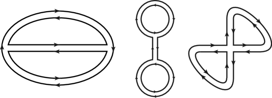
Figure 3.2. Ribbon Graphs for $g=0,s=3$

The automorphism groups of these ribbon graphs are $\mathfrak{S}_{2}\rtimes\mathbb{Z}/3\mathbb{Z}=\mathfrak{S}_{3}$, $\mathbb{Z}/2\mathbb{Z}$, and again $\mathbb{Z}/2\mathbb{Z}$, respectively. Thus the left hand side of (3.18) is

$$\frac{(-1)^{3}}{3!}+\frac{(-1)^{3}}{2}+\frac{(-1)^{2}}{2}=-\frac{1}{6}.$$

The right hand side is coming from the term $n^{3}(-z)^{1}$ of the second summation in (3.17). The value is, of course,

$$-\frac{1}{3(3-1)(3-2)}=-\frac{1}{6}.$$

It can be also computed from (3.18):

$$-\frac{(2g+s-3)!(2g)(2g-1)}{(2g)!s!}\zeta(1-2g)=\frac{(2g)(2g-1)b_{2g}}{(2g)!3!(2g)}=-\frac{1}{6}.$$

Example 3.2.

The next simple case is $g=s=1$. Since the Euler characteristic condition is the same as in Example 3.1, the only possibilities are again graphs with 1 vertex and 2 edges or 2 vertices and 3 edges. There are two ribbon graphs satisfying the conditions: Figure 2.5 and the graph on the right in Figure 2.10. The first one has $\mathfrak{S}_{2}\times\mathbb{Z}/3\mathbb{Z}$ as its automorphism group, which happens to be a degenerate case of the semi-direct product. The automorphism group of the second graph is $\mathbb{Z}/4\mathbb{Z}$, as noted in Section 2. Thus we have

$$\frac{(-1)^{3}}{6}+\frac{(-1)^{2}}{4}=\frac{1}{12}=-\zeta(-1).$$

4. KP equations and matrix integrals

There are no analytic methods of evaluating the Hermitian matrix integral

$$Z_{n}(t,m)=\int_{{\mathcal{H}}_{n}}{\text{\rm exp}}\left(-\frac{1}{2}{\text{\rm trace}}(X^{2})\right){\text{\rm exp}}\left({\text{\rm trace}}\sum_{j=3}^{2m}\frac{t_{j}}{j}X^{j}\right)\frac{d\mu(X)}{N}.$$

However, there is an interesting fact about this integral: it satisfies the system of the KP equations. In this section we give a proof of this fact.

To investigate the most general case, we define

(4.1) $$Z_{n}(t,m,\phi)=\int_{{\mathcal{H}}_{n}}{\text{\rm exp}}\left({\text{\rm trace}}\sum_{j=1}^{2m}\frac{t_{j}}{j}X^{j}\right)\phi(X)\frac{d\mu(X)}{N},$$

where $\phi(X)$ is a $U(n)$-invariant function on ${\mathcal{H}}_{n}$ which is determined by $n$ functions $\phi_{0}(k),\cdots,\phi_{n-1}(k)$ in one variable in the following manner:

(4.2) $$\phi(X)=\phi(k_{0},k_{1},\cdots k_{n-1})=\frac{\det\begin{pmatrix}\phi_{0}(k_{0})&\phi_{1}(k_{0})&\ldots&\phi_{n-1}(k_{0})\\ \phi_{0}(k_{1})&\phi_{1}(k_{1})&\ldots&\phi_{n-1}(k_{1})\\ \vdots&\vdots&\ddots&\vdots\\ \phi_{0}(k_{n-1})&\phi_{1}(k_{n-1})&\ldots&\phi_{n-1}(k_{n-1})\end{pmatrix}}{\Delta\big{(}k_{0},k_{1}\cdots,k_{n-1}\big{)}},$$

where $k_{0},\cdots,k_{n-1}$ are eigenvalues of $X$. Unlike (2.1), we allow terms containing $t_{1}X$ and $t_{2}X^{2}$ in the integral (4.1). Using (3.6), we have

$$Z_{n}(t,m,\phi)=\int_{{\mathcal{H}}_{n}}{\text{\rm exp}}\left({\text{\rm trace}}\sum_{\alpha=1}^{2m}\frac{t_{\alpha}}{\alpha}X^{\alpha}\right)\phi(X)\cdot\frac{d\mu(X)}{N}\\ =\frac{c(n)}{N}\int_{{\mathbb{R}}^{n}}{\text{\rm exp}}\left(\sum_{i=0}^{n-1}\sum_{\alpha=1}^{2m}\frac{t_{\alpha}}{\alpha}k_{i}^{\alpha}\right)\Delta(k_{0},\cdots,k_{n-1})\det\left(\phi_{j}(k_{i})\right)dk_{0}\cdots dk_{n-1}.$$

Here we need a simple formula. Let $\phi_{0}(k),\cdots,\phi_{n-1}(k)$ and $\psi_{0}(k),\cdots,\psi_{n-1}(k)$ be $2n$ arbitrary functions in $k$. Then

(4.3) $$\det\left[\phi_{i}(k_{\ell})\right]\cdot\det\left[\psi_{j}(k_{\ell})\right]=\sum_{\sigma\in{\mathfrak{S}}_{n}}\det\left[\phi_{i}(k_{\sigma(j)})\cdot\psi_{j}(k_{\sigma(j)})\right],$$

where $\sigma$ runs over all permutations of ${\mathfrak{S}}_{n}$. To prove (4.3), we calculate the left hand side by the usual product formula of the determinant. Then it becomes a summation of $n^{n}$ terms. Because of the multilinearity of the determinants, only $n!$ of these terms are nonzero. Rearranging the $n!$ terms, we obtain the above formula. Using this formula for $\psi_{j}(k)=k^{j}$, we obtain

$$\begin{split}&Z_{n}(t,m,\phi)\\ &=\frac{c(n)}{N}\int_{{\mathbb{R}}^{n}}{\text{\rm exp}}\left(\sum_{i=0}^{n-1}\sum_{\alpha=1}^{2m}\frac{t_{\alpha}}{\alpha}k_{i}^{\alpha}\right)\sum_{\sigma\in{\mathfrak{S}}_{n}}\det\left(\phi_{j}(k_{\sigma(i)})k_{\sigma(i)}^{i}\right)dk_{0}\cdots dk_{n-1}\\ &=\frac{c(n)}{N}\int_{{\mathbb{R}}^{n}}\sum_{\sigma\in{\mathfrak{S}}_{n}}{\text{\rm exp}}\left(\sum_{i=0}^{n-1}\sum_{\alpha=1}^{2m}\frac{t_{\alpha}}{\alpha}k_{\sigma(i)}^{\alpha}\right)\det\left(\phi_{j}(k_{\sigma(i)})k_{\sigma(i)}^{i}\right)dk_{0}\cdots dk_{n-1}\\ &=\frac{c(n)}{N}\sum_{\sigma\in{\mathfrak{S}}_{n}}\det\left(\int_{{\mathbb{R}}^{n}}{\text{\rm exp}}{\left(\sum_{\alpha=1}^{2m}\frac{t_{\alpha}}{\alpha}k_{\sigma(i)}^{\alpha}\right)}\phi_{j}(k_{\sigma(i)})k_{\sigma(i)}^{i}\right)dk_{0}\cdots dk_{n-1}\\ &=n!\cdot\frac{c(n)}{N}\det\left(\int_{-\infty}^{\infty}{\text{\rm exp}}{\left(\sum_{\alpha=1}^{2m}\frac{t_{\alpha}}{\alpha}k_{i}^{\alpha}\right)}\phi_{j}(k_{i})k_{i}^{i}dk_{i}\right)\\ &=n!\cdot\frac{c(n)}{N}\det\left(\int_{-\infty}^{\infty}{\text{\rm exp}}{\left(\sum_{\alpha=1}^{2m}\frac{t_{\alpha}}{\alpha}k^{\alpha}\right)}\phi_{j}(k)k^{i}dk\right).\end{split}$$

The above computation makes sense as a complex analytic function in

$$(t_{1},\cdots,t_{2m-1},t_{2m})\in{\mathbb{C}}^{2m-1}\times\{t_{2m}\in{\mathbb{C}}|Re(t_{2m})<0\},$$

on which the integral converges, provided that $|\phi_{j}(k)|$ grows slower than ${\text{\rm exp}}(k^{2m})$. To compare our $t_{j}$’s with the standard time variables in the KP theory, let us set

$$T_{\alpha}=\frac{t_{\alpha}}{\alpha}.$$

Now we use the formula

(4.4) $${\text{\rm exp}}\left(\sum_{\alpha=1}^{2m}T_{\alpha}k^{\alpha}\right)=\sum_{r=0}^{\infty}p_{r}(T)k^{r},$$

where

(4.5) $$p_{r}(T)=\sum_{n_{1}+2n_{2}+3n_{3}+\cdots+(2m)n_{2m}=r}\frac{T_{1}^{n_{1}}\cdot T_{2}^{n_{2}}\cdot T_{3}^{n_{3}}\cdots T_{2m}^{n_{2m}}}{n_{1}!\cdot n_{2}!\cdot n_{3}!\cdots n_{2m}!}$$

is a weighted homogeneous polynomial in ${\mathbb{Q}}[T_{1},\cdots,T_{2m}]$ of degree $r$. The relation (4.4) holds as an entire function in $T_{1},\cdots,T_{2m}$ and $k$. Note that we have encountered this formula already as (1.9). From (4.4), we have

$$Z_{n}(t,m,\phi)=n!\cdot\frac{c(n)}{N}\det\left(\int_{-\infty}^{\infty}\sum_{r=0}^{\infty}p_{r}(T)k^{r}\phi_{j}(k)k^{i}dk\right)\\ =n!\cdot\frac{c(n)}{N}\det\left(\int_{-\infty}^{\infty}\sum_{r=0}^{\infty}p_{r-i}(T)k^{r}\phi_{j}(k)dk\right),$$

where we define $p_{r}(T)=0$ for $r<0$.

Lemma 4.1.

Let $\phi_{j}(k)$, $j=0,\cdots,n-1$, be a function defined on ${\mathbb{R}}$ such that

$$\int_{-\infty}^{\infty}k^{r}\phi_{j}(k)dk$$

exists for all $r\geq 0$. Then as a holomorphic function defined for $Re(t_{2m})<0$, we have

$${{\mathcal{A}}}\left(\int_{-\infty}^{\infty}{\text{\rm exp}}{\left(\sum_{\alpha=1}^{2m}\frac{t_{\alpha}}{\alpha}k^{\alpha}\right)}\phi_{j}(k)k^{i}dk\right)=\sum_{r=0}^{\infty}p_{r-i}(T)\int_{-\infty}^{\infty}k^{r}\phi_{j}(k)dk$$

as $t_{2m}\rightarrow 0$.

Proof.

The argument is the same as the one we used in Section 1. We choose a fixed $t_{2m}$ so that $Re(t_{2m})<0$. Because of the uniform convergence of the power series expansion of the integrand, we can interchange the integral and the infinite sums for $\alpha=1,\cdots,2m-1$. Using (1.8), (4.4) and (4.5), we have

$$\begin{split}&{{\mathcal{A}}}\left(\int_{-\infty}^{\infty}{\text{\rm exp}}{\left(\sum_{\alpha=1}^{2m}T_{\alpha}k^{\alpha}\right)}\phi_{j}(k)k^{i}dk\right)\\ &=\sum_{n_{1}=0}^{\infty}\frac{{T_{1}}^{n_{1}}}{n_{1}!}\cdots\sum_{n_{2m}=0}^{\infty}\frac{{T_{2m}}^{n_{2m}}}{n_{2m}!}\int_{-\infty}^{\infty}k^{i+n_{1}+2n_{2}+\cdots+(2m)n_{2m}}\phi_{j}(k)dk\\ &=\sum_{r=0}^{\infty}p_{r}(T)\int_{-\infty}^{\infty}k^{i+r}\phi_{j}(k)dk.\end{split}$$

∎

Thus we have established

(4.6) $$\begin{split}{{\mathcal{A}}}\left(Z_{n}(t,m,\phi)\right)&=n!\cdot\frac{c(n)}{N}\det\left(\sum_{r=0}^{\infty}p_{r-i}(T)\int_{-\infty}^{\infty}k^{r}\phi_{j}(k)dk\right)\\ &=\det\left(\sum_{r=0}^{\infty}p_{r-i}(T)\xi_{rj}\right),\end{split}$$

where

$$\xi_{rj}=n!\cdot\frac{c(n)}{N}\int_{-\infty}^{\infty}k^{r}\phi_{j}(k)dk.$$

We recall that the determinant in (4.6) is an $n\times n$ determinant. Sato [12] proved that any size determinant of the form

(4.7) $$\det\left(\sum_{r=0}^{\infty}p_{r-i}(T)\xi_{rj}\right)$$

satisfies the Hirota bilinear form of the KP equations. He also proved that every power series solution of the KP system should be written as (4.7), allowing certain infinite determinants. A necessary background of the KP theory can be found in [7].

We have thus proved the following theorem.

Theorem 4.2.

If $\phi_{j}(k)$, $j=0,\cdots,n-1$, satisfies that

$$\left|\int_{-\infty}^{\infty}k^{r}\phi_{j}(k)dk\right|<+\infty$$

for all $r\geq 0$, then the asymptotic expansion of the matrix integral $Z_{n}(t,m,\phi)$ satisfies the KP equations with respect to $T_{1},T_{2},\cdots,T_{2m}$. Moreover, if we choose a value of $T_{2m}$ such that $Re(T_{2m})<0$ and fix it, then $Z_{n}(t,m,\phi)$ itself is an entire holomorphic solution to the KP equations with respect to $(T_{1},T_{2},\cdots,T_{2m-1})\in{{\mathbb{C}}}^{2m-1}$. In particular,

$$u(T_{1},T_{2},T_{3},\cdots)=\frac{\partial^{2}}{\partial T_{1}^{2}}\log(Z_{n}(t,m,\phi))$$

is a meromorphic solution to the KP equation

$$\frac{3}{4}u_{22}=\left(u_{3}-\frac{1}{4}u_{111}-3uu_{1}\right)_{1},$$

where $u_{j}$ denotes the partial derivative of $u$ with respect to $T_{j}$.

The formula we have just established is a continuum version of the famous Hirota soliton solution of the KP equations [12]. The most general soliton solution of the KP equations due to Mikio and Yasuko Sato depends on $nM+M$ parameters $c_{ij}$ and $\lambda_{i}$, where $0\leq i\leq M-1$ and $0\leq j\leq n-1$. Let

$$\eta(T,k)=\sum_{\alpha=1}^{2m}T_{\alpha}k^{\alpha}.$$

Then Sato-Sato’s soliton solution is given by

$$\sum_{0\leq i_{0}<\cdots<i_{n-1}\leq M-1}{\text{\rm exp}}\left(\sum_{j=0}^{n-1}\eta(T,\lambda_{i_{j}})\right)\\ \Delta(\lambda_{i_{0}},\cdots,\lambda_{i_{n-1}})\det\begin{pmatrix}c_{i_{0}0}&\ldots&c_{i_{0}n-1}\\ \vdots&&\vdots\\ c_{i_{n-1}0}&\ldots&c_{i_{n-1}n-1}\end{pmatrix}.$$

This coincides with our $Z_{n}(t,m,\phi)$ if we take

$$\phi_{j}(k)=\sum_{i=0}^{M-1}c_{ij}\delta(k-\lambda_{i}).$$

Therefore, our matrix integral $Z_{n}(t,m,\phi)$ of (4.1) with (4.2) is indeed a continuum soliton solution of the KP equations.

So far we have dealt with the matrix integrals with a fixed integer $m$ in this section. As before, we can take the limit $m\rightarrow\infty$ of these integrals, which gives formal power series solutions of the whole hierarchy of the KP equations. Note that the determinant expression of (4.6) does not have any explicit mention on the integer $m$. Therefore, we have obtained the third asymptotic formula for the matrix integral:

(4.8) $$\lim_{m\rightarrow\infty}{{\mathcal{A}}}\left(Z_{n}(t,m,\phi)\right)=n!\cdot\frac{c(n)}{N}\det\left(\sum_{r=0}^{\infty}p_{r-i}(T)\int_{-\infty}^{\infty}k^{r}\phi_{j}(k)dk\right).$$

5. Transcendental solutions of the KP equations and the Grassmannian

There are several different ways to construct solutions to the KP equations. The Krichever construction and its generalizations are based on the correspondence between certain points of the Grassmannian of Sato [12] and the algebro-geometric data consisting of an irreducible algebraic curve (possibly singular) and a torsion-free sheaf on it [6]. These solutions deserve to be called algebraic, because they carry geometric information of algebraic curves. Let us call a solution to the KP equations transcendental if no algebraic curve corresponds to this solution. The natural question we can ask is: how can we construct a transcendental solution?

In this section we show that the Hermitian matrix integrals we have been dealing with in the earlier sections are indeed transcendental solutions.

The technique we show that these matrix integrals are transcendental solutions is based on the observation that the points of the Grassmannian corresponding to these solutions satisfy a peculiar $sl(2)$ stability condition. Since these solutions are deeply related to the moduli theory of Riemann surfaces, the appearance of $sl(2)$ is mysteriously suggestive. At present we do not have any geometric explanation of the relation between the KP equations, the $sl(2)$ stability on the Grassmannian, and the moduli theory of pointed Riemann surfaces.

Let $V=\mathbb{C}((z))$ denote the field of formal Laurent series in one variable $z$. We fix its polarization

(5.1) $$\mathbb{C}((z))=\mathbb{C}[z^{-1}]\oplus\mathbb{C}[[z]]\cdot z.$$

For a vector subspace $W\subset V$, there is a natural map

(5.2) $$\gamma_{W}:W\hookrightarrow V\longrightarrow V/\mathbb{C}[[z]]z\cong\mathbb{C}[z^{-1}].$$

The infinite-dimensional Grassmannian is defined by

(5.3) $$Gr=\{W\subset V\;|\;\gamma_{W}:W\longrightarrow\mathbb{C}[z^{-1}]{\text{ is Fredholm of index }}0\}.$$

The big-cell of the Grassmannian is the subset of $Gr$ consisting of vector subspaces $W\subset V$ such that $\gamma_{W}$ of (5.2) is an isomorphism.

Let $W$ be a point of the big-cell of the Grassmannian. We can choose a basis

$$\langle w_{0},w_{1},w_{2},\cdots\rangle$$

for $W$ such that

(5.4) $$w_{j}=z^{-j}+\sum_{i=1}^{\infty}c_{ij}z^{i},\qquad j=0,1,2,\cdots.$$

The Bosonization is a map

(5.5) $$Gr\longrightarrow\mathbb{P}(\mathbb{C}[[T_{1},T_{2},T_{3},\cdots]])$$

that assigns a $\tau$-function $\tau_{W}$ to each point $W$ of the Grassmannian. For a point $W$ of the big-cell with a basis (5.4), the Bosonization has an infinite determinant expression

(5.6) $$\tau_{W}=\det\left(p_{i-j}(T)+\sum_{\mu=1}^{\infty}p_{\mu+i}(T)c_{\mu j}\right).$$

The infinite determinant gives a well-defined element of $\mathbb{C}[[T_{1},T_{2},T_{3},\cdots]]$ in the same manner as we have explained in the earlier sections. Sato’s formula (4.7) gives another expression of the Bosonization map. For more detail, we refer to [7] and [8].

The commutative stabilizer of $W\in Gr$ is defined by

(5.7) $$A_{W}=\{a\in\mathbb{C}((z))\;|\;a\cdot W\subset W\}.$$

The key idea that connects the KP equations and algebraic curves is that the commutative stabilizer is the coordinate ring of an algebraic curve. If the greatest common divisor of the pole order of elements in $A_{W}$ is $1$, then the Bosonization $\tau_{W}$ of $W$ is essentially the Riemann theta function associated with the algebraic curve $C$ whose coordinate ring is $A_{W}$ [5], [7].

Definition 5.1.

A solution of the KP equations $\tau_{W}$ is said to be transcendental if

(5.8) $$A_{W}=\mathbb{C}.$$

Remark.

It is known that if $A_{W}\neq\mathbb{C}$, then the Bosonization $\tau_{W}$ of $W$ is a solution to the KP equation corresponding to a vector bundle $\mathcal{F}$ on an algebraic curve $C$ such that

(5.9) $$H^{0}(C,\mathcal{F})=H^{1}(C,\mathcal{F})=0$$

[6]. Conversely, there is a solution corresponding to an arbitrary torsion-free sheaf $\mathcal{F}$ defined on an arbitrary (possibly singular) algebraic curve $C$ satisfying (5.9). None of these solutions are transcendental.

The Hermitian matrix integral we have discussed in Section 2 gives a transcendental solution to the KP equations.

Theorem 5.2.

Choose arbitrary positive integers $k$ and $n$, and let

$$a=(a_{1},a_{2},\cdots,a_{2k})\in\mathbb{C}^{2k}$$

be a complex vector such that $Re(a_{2k})<0$. Define a formal Laurent series

(5.10) $$w_{j}=\sum_{r=0}^{\infty}\left(\int_{-\infty}^{\infty}\lambda^{r+j}{\text{\rm exp}}\left(\sum_{\mu=1}^{2k}a_{\mu}\lambda^{\mu}\right)d\lambda\right)z^{r+1-n}\in\mathbb{C}((z))$$

for $j=0,1,2,\cdots,n-1$, and let

(5.11) $$W(a)=\langle w_{0},w_{1},\cdots,w_{n-1},z^{-n},z^{-n-1},\cdots\rangle\in Gr$$

be a point of the Grassmannian spanned by $w_{0},w_{1},\cdots,w_{n-1}$, and $z^{-n},z^{-n-1},\cdots$. Then the $\tau$-function corresponding to $W(a)$ is given by the asymptotic expansion of a Hermitian matrix integral:

(5.12) $$\tau_{W(a)}=\lim_{m\rightarrow\infty}\mathcal{A}\left(\int_{\mathcal{H}_{n}}{\text{\rm exp}}\left(\sum_{j=1}^{2m}T_{j}{\text{\rm trace}}(X^{j})\right){\text{\rm exp}}\left(\sum_{\mu=1}^{2k}a_{\mu}{\text{\rm trace}}(X^{\mu})\right)dX\right),$$

where we take $Re(T_{2m})<0$ first and then let $m\rightarrow\infty$ to determine a well-defined formal power series in $\mathbb{C}[[T_{1},T_{2},T_{3},\cdots]]$. Define a linear differential operator

(5.13) $$L_{i}(a)=z^{1-i}\frac{d}{dz}+\frac{(3n-1)+i(n-1)}{2}z^{-i}+\sum_{\mu=1}^{2k}\mu a_{\mu}z^{-i-\mu}$$

for $i=-1,0,1$. These differential operators satisfy the $sl(2,\mathbb{C})$ relation

$$[L_{i}(a),L_{j}(a)]=(i-j)L_{i+j}(a).$$

The point $W(a)$ of the Grassmannian satisfies the non-commutative stability condition

(5.14) $$L_{i}(a)\cdot W(a)\subset W(a),\qquad i=-1,0,1.$$

Moreover, $\tau_{W(a)}$ is a transcendental solution of the KP equations.

Proof.

The function

$${\text{\rm exp}}\left(\sum_{\mu=1}^{2k}a_{\mu}{\text{\rm trace}}(X^{\mu})\right)$$

is a special case of the function $\phi(X)$ defined in (4.2). Thus the results of the previous section proves that $\tau_{W(a)}$ is a $\tau$-function of the KP equations corresponding to the point of the Grassmannian $W(a)$.

Let us first prove that the $sl(2)$ stability condition (5.14) implies that the commutative stabilizer is trivial:

$$A_{W(a)}=\mathbb{C}.$$

Suppose $f(z)\in A_{W(a)}\subset\mathbb{C}((z))$, and let ${\text{\rm ord}}(f)=\nu>0$, where we define the pole order by

$${\text{\rm ord}}(z^{-\nu})=\nu.$$

Since $L_{-1}(a)$ and $f$ stabilize $W(a)$,

$$[L_{-1}(a),f]=z^{2}\frac{df}{dz}\in A_{W(a)}$$

also stabilizes $W(a)$. Note that

$${\text{\rm ord}}([L_{-1}(a),f])=\nu-1.$$

Thus we can immediately conclude that

$$A_{W(a)}=\mathbb{C}[z^{-1}].$$

But then

(5.15) $$L_{-1}(a)-\sum_{\mu=1}^{2k}\mu a_{\mu}z^{1-\mu}=z^{2}\frac{d}{dz}+\frac{(3n-1)-(n-1)}{2}z$$

stabilizes $W(a)$. Since the new stabilizer (5.15) decreases the order of elements of $W(a)$ exactly by $1$, $W(a)$ must have an element of arbitrary negative order. But this contradicts to the Fredholm condition of $W(a)$. This means $A_{W(a)}=\mathbb{C}$, hence $\tau_{W(a)}$ is a transcendental solution.

Now all we need is to show (5.14), which can be verified by a straightforward computation. First, we note a simple formula

(5.16) $$\begin{split}0&=\int_{-\infty}^{\infty}\frac{d}{d\lambda}\left(\lambda^{\alpha}{\text{\rm exp}}\left(\sum_{\mu=1}^{2k}a_{\mu}\lambda^{\mu}\right)d\lambda\right)\\ &=\int_{-\infty}^{\infty}\alpha\lambda^{\alpha-1}{\text{\rm exp}}\left(\sum_{\mu=1}^{2k}a_{\mu}\lambda^{\mu}\right)d\lambda\\ &\quad+\int_{-\infty}^{\infty}\sum_{\mu=1}^{2k}\mu a_{\mu}\lambda^{\alpha+\mu-1}{\text{\rm exp}}\left(\sum_{\mu=1}^{2k}a_{\mu}\lambda^{\mu}\right)d\lambda.\\ \end{split}$$

Let us compute the effect of the differential operators (5.13) on the basis elements of $W(a)$. First, we have

$$L_{-1}(a)w_{j}=\left(z^{2}\frac{d}{dz}+nz+\sum_{\mu=1}^{2k}\mu a_{\mu}z^{1-\mu}\right)\sum_{r=0}^{\infty}z^{r+1-n}\int_{-\infty}^{\infty}\lambda^{r+j}e^{\sum_{\mu=1}^{2k}a_{\mu}\lambda^{\mu}}d\lambda\\ =\sum_{r=0}^{\infty}(r+1)z^{r+2-n}\int_{-\infty}^{\infty}\lambda^{r+j}e^{\sum_{\mu=1}^{2k}a_{\mu}\lambda^{\mu}}d\lambda\\ \qquad+\sum_{r=0}^{\infty}\sum_{\mu=1}^{2k}z^{r+2-n-\mu}\int_{-\infty}^{\infty}\lambda^{r+j}\mu a_{\mu}e^{\sum_{\mu=1}^{2k}a_{\mu}\lambda^{\mu}}d\lambda\\ =\sum_{r=0}^{\infty}rz^{r+1-n}\int_{-\infty}^{\infty}\lambda^{r+j-1}e^{\sum_{\mu=1}^{2k}a_{\mu}\lambda^{\mu}}d\lambda\\ \qquad+\sum_{\mu=1}^{2k}\sum_{r=0}^{\mu-2}z^{r+2-n-\mu}\int_{-\infty}^{\infty}\lambda^{r+j}\mu a_{\mu}e^{\sum_{\mu=1}^{2k}a_{\mu}\lambda^{\mu}}d\lambda\\ \qquad+\sum_{\mu=1}^{2k}\sum_{r=\mu-1}^{\infty}z^{r+2-n-\mu}\int_{-\infty}^{\infty}\lambda^{r+j}\mu a_{\mu}e^{\sum_{\mu=1}^{2k}a_{\mu}\lambda^{\mu}}d\lambda\\ =\sum_{r=0}^{\infty}rz^{r+1-n}\int_{-\infty}^{\infty}\lambda^{r+j-1}e^{\sum_{\mu=1}^{2k}a_{\mu}\lambda^{\mu}}d\lambda\\ \qquad+\sum_{\mu=1}^{2k}\sum_{r=0}^{\mu-2}z^{r+2-n-\mu}\int_{-\infty}^{\infty}\lambda^{r+j}\mu a_{\mu}e^{\sum_{\mu=1}^{2k}a_{\mu}\lambda^{\mu}}d\lambda\\ \qquad+\sum_{\mu=1}^{2k}\sum_{r=0}^{\infty}z^{r+1-n}\int_{-\infty}^{\infty}\lambda^{r+j+\mu-1}\mu a_{\mu}e^{\sum_{\mu=1}^{2k}a_{\mu}\lambda^{\mu}}d\lambda\\ =\sum_{r=0}^{\infty}rz^{r+1-n}\int_{-\infty}^{\infty}\lambda^{r+j-1}e^{\sum_{\mu=1}^{2k}a_{\mu}\lambda^{\mu}}d\lambda\\ \qquad+\sum_{\mu=1}^{2k}\sum_{r=0}^{\mu-2}z^{r+2-n-\mu}\int_{-\infty}^{\infty}\lambda^{r+j}\mu a_{\mu}e^{\sum_{\mu=1}^{2k}a_{\mu}\lambda^{\mu}}d\lambda\\ \qquad-\sum_{r=0}^{\infty}z^{r+1-n}\int_{-\infty}^{\infty}(r+j)\lambda^{r+j-1}e^{\sum_{\mu=1}^{2k}a_{\mu}\lambda^{\mu}}d\lambda\\ =-jw_{j-1}+\sum_{\mu=1}^{2k}\sum_{r=0}^{\mu-2}z^{r+2-n-\mu}\int_{-\infty}^{\infty}\lambda^{r+j}\mu a_{\mu}e^{\sum_{\mu=1}^{2k}a_{\mu}\lambda^{\mu}}d\lambda\\ \in W(a)\\$$

for all $j=0,1,2,\cdots,n-1$. Note that $w_{-1}$ does not appear in the above computation because of the combination $jw_{j-1}$. For the basis elements $z^{-n},z^{-n-1},\cdots,$ we have

$$\begin{split}L_{-1}(a)z^{-n-i}&=\left(z^{2}\frac{d}{dz}+nz+\sum_{\mu=1}^{2k}\mu a_{\mu}z^{1-\mu}\right)z^{-n-i}\\ &=(-i)z^{-n-i+1}+\sum_{\mu=1}^{2k}\mu a_{\mu}z^{1-\mu-n-i}\in W(a)\\ \end{split}$$

for all $i\geq 0$. We note that the term $z^{-n+1}$ does not appear in this computation. Thus we conclude

$$L_{-1}(a)\cdot W(a)\subset W(a).$$

For $j=0$, we have

$$L_{0}(a)w_{j}=\left(z\frac{d}{dz}+\frac{3n-1}{2}+\sum_{\mu=1}^{2k}\mu a_{\mu}z^{-\mu}\right)\sum_{r=0}^{\infty}z^{r+1-n}\int_{-\infty}^{\infty}\lambda^{r+j}e^{\sum_{\mu=1}^{2k}a_{\mu}\lambda^{\mu}}d\lambda\\ =\sum_{r=0}^{\infty}(r+\frac{n+1}{2})z^{r+1-n}\int_{-\infty}^{\infty}\lambda^{r+j}e^{\sum_{\mu=1}^{2k}a_{\mu}\lambda^{\mu}}d\lambda\\ \qquad+\sum_{r=0}^{\infty}\sum_{\mu=1}^{2k}z^{r+1-n-\mu}\int_{-\infty}^{\infty}\lambda^{r+j}\mu a_{\mu}e^{\sum_{\mu=1}^{2k}a_{\mu}\lambda^{\mu}}d\lambda\\ =\frac{n+1}{2}w_{j}+\sum_{r=0}^{\infty}rz^{r+1-n}\int_{-\infty}^{\infty}\lambda^{r+j}e^{\sum_{\mu=1}^{2k}a_{\mu}\lambda^{\mu}}d\lambda\\ \qquad+\sum_{\mu=1}^{2k}\sum_{r=0}^{\mu-1}z^{r+1-n-\mu}\int_{-\infty}^{\infty}\lambda^{r+j}\mu a_{\mu}e^{\sum_{\mu=1}^{2k}a_{\mu}\lambda^{\mu}}d\lambda\\ \qquad+\sum_{\mu=1}^{2k}\sum_{r=\mu}^{\infty}z^{r+1-n-\mu}\int_{-\infty}^{\infty}\lambda^{r+j}\mu a_{\mu}e^{\sum_{\mu=1}^{2k}a_{\mu}\lambda^{\mu}}d\lambda\\ =\frac{n+1}{2}w_{j}+\sum_{r=0}^{\infty}rz^{r+1-n}\int_{-\infty}^{\infty}\lambda^{r+j}e^{\sum_{\mu=1}^{2k}a_{\mu}\lambda^{\mu}}d\lambda\\ \qquad+\sum_{\mu=1}^{2k}\sum_{r=0}^{\mu-1}z^{r+1-n-\mu}\int_{-\infty}^{\infty}\lambda^{r+j}\mu a_{\mu}e^{\sum_{\mu=1}^{2k}a_{\mu}\lambda^{\mu}}d\lambda\\ \qquad+\sum_{\mu=1}^{2k}\sum_{r=0}^{\infty}z^{r+1-n}\int_{-\infty}^{\infty}\lambda^{r+j+\mu}\mu a_{\mu}e^{\sum_{\mu=1}^{2k}a_{\mu}\lambda^{\mu}}d\lambda\\ =\frac{n+1}{2}w_{j}+\sum_{r=0}^{\infty}rz^{r+1-n}\int_{-\infty}^{\infty}\lambda^{r+j}e^{\sum_{\mu=1}^{2k}a_{\mu}\lambda^{\mu}}d\lambda\\ \qquad+\sum_{\mu=1}^{2k}\sum_{r=0}^{\mu-1}z^{r+1-n-\mu}\int_{-\infty}^{\infty}\lambda^{r+j}\mu a_{\mu}e^{\sum_{\mu=1}^{2k}a_{\mu}\lambda^{\mu}}d\lambda\\ \qquad-\sum_{r=0}^{\infty}z^{r+1-n}\int_{-\infty}^{\infty}(r+j+1)\lambda^{r+j}e^{\sum_{\mu=1}^{2k}a_{\mu}\lambda^{\mu}}d\lambda\\ =\left(\frac{n+1}{2}-j-1\right)w_{j}+\sum_{\mu=1}^{2k}\sum_{r=0}^{\mu-1}z^{r+1-n-\mu}\int_{-\infty}^{\infty}\lambda^{r+j}\mu a_{\mu}e^{\sum_{\mu=1}^{2k}a_{\mu}\lambda^{\mu}}d\lambda\\ \in W(a)\\$$

for all $j=0,1,2,\cdots,n-1$. It is obvious that

$$L_{0}(a)\cdot z^{-n-i}\in W(a)$$

for $i\geq 0$. Finally, for $j=1$, we have

$$L_{1}(a)w_{j}\\ =\left(\frac{d}{dz}+(2n-1)z^{-1}+\sum_{\mu=1}^{2k}\mu a_{\mu}z^{-\mu-1}\right)\sum_{r=0}^{\infty}z^{r+1-n}\int_{-\infty}^{\infty}\lambda^{r+j}e^{\sum_{\mu=1}^{2k}a_{\mu}\lambda^{\mu}}d\lambda\\ =\sum_{r=0}^{\infty}(r+n)z^{r-n}\int_{-\infty}^{\infty}\lambda^{r+j}e^{\sum_{\mu=1}^{2k}a_{\mu}\lambda^{\mu}}d\lambda\\ \qquad+\sum_{r=0}^{\infty}\sum_{\mu=1}^{2k}z^{r-n-\mu}\int_{-\infty}^{\infty}\lambda^{r+j}\mu a_{\mu}e^{\sum_{\mu=1}^{2k}a_{\mu}\lambda^{\mu}}d\lambda\\ =\sum_{r=-1}^{\infty}(r+n+1)z^{r+1-n}\int_{-\infty}^{\infty}\lambda^{r+j+1}e^{\sum_{\mu=1}^{2k}a_{\mu}\lambda^{\mu}}d\lambda\\ \qquad+\sum_{\mu=1}^{2k}\sum_{r=0}^{\mu}z^{r-n-\mu}\int_{-\infty}^{\infty}\lambda^{r+j}\mu a_{\mu}e^{\sum_{\mu=1}^{2k}a_{\mu}\lambda^{\mu}}d\lambda\\ \qquad+\sum_{\mu=1}^{2k}\sum_{r=\mu+1}^{\infty}z^{r-n-\mu}\int_{-\infty}^{\infty}\lambda^{r+j}\mu a_{\mu}e^{\sum_{\mu=1}^{2k}a_{\mu}\lambda^{\mu}}d\lambda\\ =z^{-n}\int_{-\infty}^{\infty}\lambda^{j}e^{\sum_{\mu=1}^{2k}a_{\mu}\lambda^{\mu}}d\lambda+\sum_{r=0}^{\infty}(r+n+1)z^{r+1-n}\int_{-\infty}^{\infty}\lambda^{r+j+1}e^{\sum_{\mu=1}^{2k}a_{\mu}\lambda^{\mu}}d\lambda\\ \qquad+\sum_{\mu=1}^{2k}\sum_{r=0}^{\mu}z^{r-n-\mu}\int_{-\infty}^{\infty}\lambda^{r+j}\mu a_{\mu}e^{\sum_{\mu=1}^{2k}a_{\mu}\lambda^{\mu}}d\lambda\\ \qquad+\sum_{\mu=1}^{2k}\sum_{r=0}^{\infty}z^{r+1-n}\int_{-\infty}^{\infty}\lambda^{r+j+\mu+1}\mu a_{\mu}e^{\sum_{\mu=1}^{2k}a_{\mu}\lambda^{\mu}}d\lambda\\ =z^{-n}\int_{-\infty}^{\infty}\lambda^{j}e^{\sum_{\mu=1}^{2k}a_{\mu}\lambda^{\mu}}d\lambda+\sum_{r=0}^{\infty}(r+n+1)z^{r+1-n}\int_{-\infty}^{\infty}\lambda^{r+j+1}e^{\sum_{\mu=1}^{2k}a_{\mu}\lambda^{\mu}}d\lambda\\ \qquad+\sum_{\mu=1}^{2k}\sum_{r=0}^{\mu}z^{r-n-\mu}\int_{-\infty}^{\infty}\lambda^{r+j}\mu a_{\mu}e^{\sum_{\mu=1}^{2k}a_{\mu}\lambda^{\mu}}d\lambda\\ \qquad-\sum_{r=0}^{\infty}z^{r+1-n}\int_{-\infty}^{\infty}(r+j+2)\lambda^{r+j+1}e^{\sum_{\mu=1}^{2k}a_{\mu}\lambda^{\mu}}d\lambda\\ =z^{-n}\int_{-\infty}^{\infty}\lambda^{j}e^{\sum_{\mu=1}^{2k}a_{\mu}\lambda^{\mu}}d\lambda+(n-j-1)w_{j+1}\\ \qquad+\sum_{\mu=1}^{2k}\sum_{r=0}^{\mu}z^{r-n-\mu}\int_{-\infty}^{\infty}\lambda^{r+j}\mu a_{\mu}e^{\sum_{\mu=1}^{2k}a_{\mu}\lambda^{\mu}}d\lambda\\ \in W(a)\\$$

for all $j=0,1,2,\cdots,n-1$. Note that the term $w_{n}$ does not appear in the computation. It is again obvious that

$$L_{1}(a)\cdot z^{-n-i}\in W(a)$$

for $i\geq 0$. This completes the proof of the $sl(2)$ stability of $W(a)$, and hence we have established the theorem. ∎

The action of these $sl(2)$ generators on $W(a)$ is very subtle, and it does not seem to allow any generalization. For example, the above proof does not apply for the Virasoro generators $L_{i}(a)$ other than $i=-1,0,1$, although the operators $L_{i}(a)$ are defined for all $i\in\mathbb{Z}$ and they satisfy the Witt algebra relation

$$[L_{i}(a),L_{j}(a)]=(i-j)L_{i+j}(a)$$

for $i,j\in\mathbb{Z}$.

References

[1]
Enrico Arbarello and C. De Concini.
On a set of equations characterizing the Riemann matrices.
Annals of Mathematics, 120:119–140, 1984.
[2]
D. Bessis, C. Itzykson, and J. B. Zuber.
Quantum field theory techniques in graphical enumeration.
Advances in Applied Mathematics, 1:109–157, 1980.
[3]
J. Harer and D. Zagier.
The Euler characteristic of the moduli space of curves.
Inventiones Mathematicae, 85:457–485, 1986.
[4]
Maxim Kontsevich.
Intersection theory on the moduli space of curves and the matrix
Airy function.
Communications in Mathematical Physics, 147:1–23, 1992.
[5]
Motohico Mulase.
Cohomological structure in soliton equations and jacobian varieties.
Journal of Differential Geometry, 19:403–430, 1984.
[6]
Motohico Mulase.
Category of vector bundles on algebraic curves and infinite
dimensional Grassmannians.
International Journal of Mathematics, 1:293–342, 1990.
[7]
Motohico Mulase.
Algebraic theory of the KP equations.
In Robert C. Penner and Shing-Tung Yau, editors, Perspectives in
Mathematical Physics, pages 151–217. International Press Inc., 1994.
[8]
Motohico Mulase.
Matrix integrals and integrable systems.
In K. Fukaya, M. Furuta, T. Kohno, and D. Kotschick, editors, Topology, Geometry and Field Theory, pages 111–127. World Scientific
Publishing Co., 1994.
[9]
Motohico Mulase.
Asymptotic analysis of a hermitian matrix integral.
International Journal of Mathematics, 6:881–892, 1995.
[10]
David Mumford.
An algebro-geometric constructions of commuting operators and of
solutions to the Toda lattice equations, Korteweg-de Vries equations
and related nonlinear equations.
In Proceedings of the International Symposium on Algebraic
Geometry, Kyoto 1977, pages 115–153. Kinokuniya Publishers, 1978.
[11]
Robert C. Penner.
Perturbation series and the moduli space of Riemann surfaces.
Journal of Differential Geometry, 27:35–53, 1988.
[12]
Mikio Sato.
Soliton equations as dynamical systems on an infinite-dimensional
Grassmann manifold.
Kokyuroku of the Research Institute for Mathematical Sciences,
Kyoto University, 439:30–46, 1981.
[13]
Takahiro Shiota.
Characterization of jacobian varieties in terms of soliton equations.
Inventiones Mathematicae, 83:333–382, 1986.
[14]
G. ’tHooft.
A planer diagram theory for strong interactions.
Nuclear Physics B, 72:461–473, 1974.
[15]
Edward Witten.
Two dimensional gravity and intersection theory on moduli space.
Surveys in Differential Geometry, 1:243–310, 1991.