The Significance of the $C$-Numerical Range and
the Local $C$-Numerical Range in Quantum Control and Quantum Information

Zusammenfassung

This paper shows how $C$-numerical-range related new strucures may arise from practical problems in quantum control—and vice versa, how an understanding of these structures helps to tackle hot topics in quantum information.

We start out with an overview on the role of $C$-numerical ranges in current research problems in quantum theory: the quantum mechanical task of maximising the projection of a point on the unitary orbit of an initial state onto a target state $C$ relates to the $C$-numerical radius of $A$ via maximising the trace function $|\operatorname{tr}\{C^{\dagger}UAU^{\dagger}\}|$. In quantum control of $n$ qubits one may be interested (i) in having $U\in SU(2^{n})$ for the entire dynamics, or (ii) in restricting the dynamics to local operations on each qubit, i.e. to the $n$-fold tensor product $SU(2)\otimes SU(2)\otimes\cdots\otimes SU(2)$. Interestingly, the latter then leads to a novel entity, the local $C$-numerical range $W_{\rm loc}(C,A)$, whose intricate geometry is neither star-shaped nor simply connected in contrast to the conventional $C$-numerical range. This is shown in the accompanying paper on Relative $C$-Numerical Ranges for Application in Quantum Control and Quantum Information [1]. We present novel applications of the $C$-numerical range in quantum control assisted by gradient flows on the local unitary group: (1) they serve as powerful tools for deciding whether a quantum interaction can be inverted in time (in a sense generalising Hahn’s famous spin echo); (2) they allow for optimising witnesses of quantum entanglement. We conclude by relating the relative $C$-numerical range to problems of constrained quantum optimisation, for which we also give Lagrange-type gradient flow algorithms.

We are currently in the midst of a second quantum revolution. The
first one gave us new rules that govern physical reality. The second
one will take these rules and  use them to develop new technologies.
X                                                   Dowling and Milburn, 2003 [2]

It was the main goal of the talk entailing this paper to entice the numerical range community to showing further interest in problems of optimisation and control of quantum systems. By illustrating how important properties of $C$-numerical ranges relate to reachability and optimisation in quantum dynamics, we wish to foster cross-fertilisation leading—in turn—also to new discoveries in numerical ranges. These may go beyond or follow earlier work on applying higher-rank numerical ranges [3] to quantum error correction [4], or numerical ranges of derivations to anti-symmetric quantum states [5], on optimising coherence transfer in quantum systems [6, 7, 8], which entailed special interest in the $C$-numerical range of nilpotent matrices relevant in spectroscopy [9, 10]. As contribution to our end, we present some new results on what we introduce as relative $C$-numerical range [1], we relate some of our recent results in quantum control to numerical ranges, and we express corner stones of quantum control in the setting of numerical ranges. A reader interested in the quantum aspects may appreciate the paper being organised such as to pursue these issues in reverse order, whereas the one driven by impatient curiosity may prefer to jump into Section 1.5 or Chapters 2 and 3 right away.

1 Overview on $C$-Numerical Ranges in Quantum Control

Controlling quantum systems offers a great potential for performing computational tasks or for simulating the behaviour of other quantum systems [11, 12]. This is because the complexity of many problems [13] reduces upon going from classical to quantum hardware. It roots in Feynman’s observation [11] that the resources required for simulating a quantum system on a classical computer increase exponentially with the system size. In turn, he concluded that using quantum hardware might therefore exponentially decrease the complexity of certain classical computation problems. Coherent superpositions of quantum states used as so-called ‘qubits’ can be viewed as a particularly powerful resource of quantum parallelism unparalleled by any classical system. Important applications are meanwhile known in quantum computation, quantum search and quantum simulation: most prominently, there is the exponential speed-up by Shor’s quantum algorithm of prime factorisation [14, 15], which relates to the general class of quantum algorithms [16, 17] solving hidden subgroup problems in an efficient way [18].

However, for exploiting the power of quantum systems, one has to steer them by classical controls such as voltage gates, radio-frequency pulses, or laser beams. It is highly desirable to do so in an optimal way, because the shapes of these controls critically determine the performance of the quantum system in terms of overlap of its actual final states with the desired target states. Here, the aim is to show how quantum optimal control relates to finding points on the unitary orbit of the initial quantum state $A$ (in its density matrix representation) maximally projecting onto the desired target state $C$ which is equivalent to maximising the target function

$$F(U)=|\operatorname{tr}\{UAU^{\dagger}C^{\dagger}\}|$$ (1)

over all unitaries to yield the $C$-numerical radius of $A$. This is the scope in systems that are fully controllable in the sense that every propagator $U\in SU(2^{n})$ can be realised on the physical system in question.

Yet, often only local unitary operations $K\in SU(2)\otimes SU(2)\otimes\cdots\otimes SU(2)$ are actually available. Then the corresponding optimisation problems are confined to a subset of the conventional $C$-numerical range: this is the motivation to introduce the local $C$-numerical range $W_{\rm loc}(C,A)$ as a special case of the relative $C$-numerical range $W_{\mathbf{K}}(C,A)$, whose intricate geometry is analysed in more detail in the accompanying paper [1].

In view of practical applications in quantum control, we finally give an outlook on contrained optimisation problems, i.e., those in which extremal points in the $C$-numerical range are searched subject to fulfilling contraints such as keeping $UAU^{\dagger}$ orthogonal to an undesired state $D$ or leaving a neutral state $E$ invariant.

Since in general, a precise characterisation of solutions in algebraic terms is often beyond reach, we resort to numerical methods based on gradient flows on the unitary group.

1.1 Quantum Dynamics: Notations and Relation to $C$-Numerical Range

As usual in quantum mechanics, one may choose to represent a state of a pure quantum system by a state vector in Hilbert space, $|\psi\rangle{}\in\mathcal{H}$. Its norm induced by the scalar product can be set to $\langle\psi|\psi\rangle{}=1$, as will be assumed henceforth. The operators associated to quantum mechanical observables such as the Hamiltonian $H$ are selfadjoint, so $H=H^{\dagger}$. Then the Hamiltonian dynamics is governed by Schrödinger’s equation of motion

$$|\dot{\psi}(t)\rangle{}=-iH\;|\psi(t)\rangle{}\quad\text{solved by}\quad|\psi(t)\rangle{}=e^{-itH}\;|\psi(0)\rangle{}={U(t)}\;|\psi(0)\rangle{}\;.$$ (2)

Invoking Stone-von Neumann’s theorem, the solution involves a time evolution by an element $U(t)$ of the strongly continuous one-parameter group $\mathcal{U}:=\{e^{-itH}\,|\,t\in\mathbb{R}^{\,}{}\}$ generated by the Hamiltonian $H$, see e.g. [19].

Non-pure quantum states comprise the settings of classically mixed states as well as reduced representations of quantum systems allowing for the description of open dissipative systems. In these cases, one may choose to represent the state by a positive-semidefinite trace-class operator, the density operator $\rho\in\mathcal{B}_{1}(\mathcal{H})$ with $\rho\geq 0$ being normalised to $\operatorname{tr}\rho=1$. With the trace-class operators $\mathcal{B}_{1}(\mathcal{H})$ forming a two-sided ideal in the bounded ones $\mathcal{B}(\mathcal{H})$, its dynamics follows Liouville-von Neumann’s equation

$$\dot{\rho}(t)=-i[H,\rho(t)]\quad\text{solved by}\quad\rho(t)={U}(t)\rho(0){U(t)^{\dagger}}\quad,\quad U(t)=e^{-itH}$$ (3)

and thus ‘dwells’ on the unitary orbit of the initial state $\mathcal{O}_{u}\big{(}\rho(0)\big{)}$.

Next, consider the expectation value of observables $B=B^{\dagger}\in\mathcal{B}(\mathcal{H})$ in either setting. For pure quantum states it takes the form of the scalar product $\langle\cdot|\cdot\rangle{}$

$$\langle B\rangle{}(t):=\langle\psi(t)B|\psi(t)\rangle{}$$ (4)

while for non-pure states (using the Hilbert-Schmidt analogue $\operatorname{tr}\{\cdot^{\dagger}\cdot\}$) it reads

$$\langle\langle B\rangle{}\rangle{}(t)=\operatorname{tr}\big{(}B^{\dagger}\rho(t)\big{)}=\operatorname{tr}\big{(}B^{\dagger}\;U(t)\rho(0)U(t)^{\dagger}\big{)}\quad.$$ (5)

Clearly, in pure states the expectation value is an element of the field of values $\langle B\rangle{}(t)\in W(B):=\{\langle u|Bu\rangle{}\,\big{|}\|u\|{}=1\}$, whereas in non-pure states it is an element of the $C$-numerical range $\langle\langle B\rangle{}\rangle{}(t)\in W(B,\rho(0))$ then taking the form of a real line segment. The latter is of particular significance, e.g., in ensemble spectroscopy, where it is customary to collect all signal-relevant components of the selfadjoint operator $B$ in a new operator $C$ that need no longer be Hermitian, and likewise the pertinent terms of $\rho(0)$ in a general complex operator $A$. Thus moving from the selfadjoint operators $B,\rho$ to arbitrary, not necessarily Hermitian (yet bounded) operators $A,C$, the analogue to the ensemble expectation value then becomes a general element of the $C$-numerical range $W(C,A):=\{\operatorname{tr}(C^{\dagger}\;UAU^{\dagger})|U\in\mathcal{U}(\mathcal{H})\}$, where here and henceforth $A,C\in\operatorname{Mat}{}_{n}(\mathbb{C}^{\,}{})$ are taken to be finite-dimensional in view of spin and pseudo-spin systems.

The key features of $W(C,A)$ [20, 21] may thus be exploited for quantum optimisation and control. They comprise: (i) the $C$-spectrum of $A$ is a subset of $W(C,A)$; (ii) $W(C,A)$ is always compact, connected and star-shaped [22] with respect to the centre $\operatorname{tr}\{A\}\operatorname{tr}\{C^{\dagger}\}/N$; it is convex if (but not only if) $C$ is normal with collinear eigenvalues in the complex plane, or if there is a $\mu\in\mathbb{C}^{\,}{}$ so that $(C-\mu{\rm 1\negthickspace l}{})$ has rank 1; it is a circular disc in the complex plane [23] if there is a $\mu\in\mathbb{C}^{\,}{}$ so that $(C-\mu{\rm 1\negthickspace l}{})$ is unitarily similar to block-shift form; (iii) the corners of the boundary $\partial{W(C,A)}$ at which no tangent exists are always elements of the $C$-spectrum of $A$; (iv) for normal $C$ with collinear eigenvalues in the complex plane (as well as in some degenerate cases [21]) $W(C,A)$ is the closed convex hull of the $C$-spectrum of $A$ thus forming a convex polygonal disc in the complex plane.

1.2 Geometry of Optimisation within $C$-Numerical Ranges

In the context of $C$-numerical ranges, there are geometric optimisation tasks immediately related to problems of quantum control, e.g., finding points on the unitary orbit of (the initial state) $A$ that

1. show a minimum Euclidean distance to (the target state) $C$ corresponds to the maximum real part of the $C$-numerical range by

   $${||C-UAU^{\dagger}||}_{2}^{2}={||A||}_{2}^{2}+{||C||}_{2}^{2}-2\operatorname{Re}\operatorname{tr}\{C^{\dagger}\;UAU^{\dagger}\}\quad,$$ (6)

   while those that

2. enclose a minimal angle (mod $\pi$) to $C$ relate to the $C$-numerical radius $r(C,A):=\underset{U}{\max}|\operatorname{tr}\{C^{\dagger}UAU^{\dagger}\}|$ by

   $$\cos^{2}_{A,C}\,(U)=\frac{|\operatorname{tr}\{C^{\dagger}UAU^{\dagger}\}|^{2}}{{\|A\|}_{2}^{2}\cdot{\|C\|}_{2}^{2}}\quad.$$ (7)

Clearly, the mathematical limits to unitary transfer from $A$ onto $C$ are physically meaningful only if all the transformations in the entire unitary group can be realised in the given experimental setting. This is what we will analyse in the next section.— In a fully controllable system, the $C$-numerical radius coincides with the maximal transfer of relevant components collected in $A$ onto the target $C$. In coherent ensemble spectroscopy, this is identical to the maximal spectroscopic signal amplitudes obtainable in the absence of relaxation [6, 7].

1.3 Controllability of Quantum Systems

The standard bilinear control system with state $X(t)$, drift $A$, controls $B_{j}$, and control amplitudes $u_{j}\in\mathbb{R}^{\,}{}$ reads

$$\dot{X}(t)=\big{(}A+\sum_{j=1}^{m}u_{j}(t)B_{j}\big{)}\;X(t)\quad,$$ (8)

while $X(t)\in\mathcal{GL}_{N}(\mathbb{C}^{\,}{})$ and $A,B_{j}\in\operatorname{Mat}{}_{N}(\mathbb{C}^{\,}{})$. Thus Hamiltonian quantum dynamics following Schrödinger’s equation

$$|\dot{\psi}(t)\rangle{} = -i\big{(}H_{d}+\sum_{j=1}^{m}u_{j}(t)H_{j}\big{)}\;|\psi(t)\rangle{}$$ (9)

$${\dot{U}(t)} = -i\big{(}H_{d}+\sum_{j=1}^{m}u_{j}(t)H_{j}\big{)}\;{U(t)}\quad,$$ (10)

can be cast into the above setting. Here $H_{d}$ is the drift term, $H_{j}$ are the control Hamiltonians with $u_{j}(t)$ as control amplitudes. For $n$ qubits, $|\psi\rangle{}\in\mathbb{C}^{\,2^{n}}{}$, $U\in SU(2^{n})$, and $i\,H_{\nu}\in\mathfrak{su}(2^{n})$.

Definition 1.1 ((Full Controllability)).

A system is fully controllable, if to every initial state $A$ the entire unitary orbit $\mathcal{O}_{u}(A)$ can be reached.

In the special case of Hermitian operators this means any final state $X(t)=:C$ can be reached from any initial state $X(0)=:A$ as long as the operators $A$ and $C$ share the same spectrum of eigenvalues.

Corollary 1.2.

[24]
The bilinear system of Eqn. 10 is fully controllable if and only if drift and controls are a generating set of $\mathfrak{su}(2^{n})$ by way of the commutator, in the sense $\langle{H_{d},H_{j}}\,|\,j=1,2,\dots,m\rangle_{\rm Lie}={\mathfrak{su}(2^{n})}$.

Example 1.3 (($n$ weakly coupled spin-$\tfrac{1}{2}$ qubits):).

Let $\sigma_{x}=\left(\begin{smallmatrix}\,0&\,1\,\\ \,1&\,0\,\end{smallmatrix}\right)$, $\sigma_{y}=\left(\begin{smallmatrix}0&-i\\ i&\phantom{-}0\end{smallmatrix}\right)$, $\sigma_{z}=\left(\begin{smallmatrix}1&\phantom{-}0\\ 0&-1\end{smallmatrix}\right)$ be the Pauli matrices. In $n$ spins-$\tfrac{1}{2}$, a $\sigma_{kx}$ for spin $k$ is tacitly embedded as ${\rm 1\negthickspace l}{}\otimes\cdots{\rm 1\negthickspace l}{}\otimes\sigma_{x}\otimes{\rm 1\negthickspace l}{}\otimes\cdots{\rm 1\negthickspace l}{}$ where $\sigma_{x}$ is at position $k$. The same holds for $\sigma_{ky}$, $\sigma_{kz}$, and in the weak coupling terms $\sigma_{kz}\sigma_{\ell z}$ with $1\leq k<\ell\leq n$.

Theorem 1.4 ((Controllability of Coupled Qubits)).

[7]
A system of $n$ qubits is fully controllable, if e.g. the control Hamiltonians $H_{j}$ comprise the Pauli matrices $\{{\sigma_{kx},\sigma_{ky}}\,|\,k=1,2,\dots n\}$ on every single qubit selectively and the drift Hamiltonian $H_{d}$ encompasses the Ising pair interactions $\{{J_{k\ell}}\;{(\sigma_{kz}\sigma_{\ell z})/2}\,|\,k<\ell=2,\dots n\}$, where the coupling topology of $J_{k\ell}\neq 0$ may take the form of any connected graph.

This theorem has meanwhile been generalised to other types of couplings [25, 26].

Example 1.5 ((Quantum Gates)).

:
In quantum computing, the logical gate operations have a unitary representation. Therefore, implementing a unitary gate by a sequence of evolutions under drift and control terms of the respective hardware (i.e., the physical quantum system) can be seen as the quantum compilation task: it translates the unitary gates into the machine code of physically accessible controls.

Corollary 1.6.

The following are equivalent:

1. in a quantum system of $n$ coupled spins-$\tfrac{1}{2}$, the drift $H_{d}$ and the controls $H_{j}$ form a generating set of $\mathfrak{su}(2^{n})$;

2. every unitary transformation $U\in SU(2^{n})$ can be realised by that system;

3. there is a set of universal quantum gates for the quantum system;

4. the quantum system is fully controllable;

5. the reachability set to the generalised expectation value $\langle\langle C\rangle{}\rangle{}(t)=\operatorname{tr}\{C^{\dagger}A(t)\}$ coincides with the $C$-numerical range $W(C,A)$ for all $A,C\in\operatorname{Mat}{}_{2^{n}}(\mathbb{C}^{\,}{})$.

Proof 1.7.

: (1) $\Leftrightarrow$ (2) follows by using the surjectivity of the exponential map in compact connected groups [24]; (2) $\Leftrightarrow$ (3) express the same fact in the terminology of group theory (2) and quantum computing (3); (4) $\Leftrightarrow$ (1) follows by Corollary 1.2; (4) $\Leftrightarrow$ (5) by definition of full controllability via reachability of the entire unitary orbit $\mathcal{O}_{u}(A)$.

1.4 Tasks in Optimal Quantum Control

‘Optimise a scalar quality function subject to the equation of motion governing the dynamics of the system to be steered’–this is the formal setting of many an engineering problem both in classical and quantum systems.

Extending the notions of quantum dynamics introduced above in Sec. 1.1, there are two principle types of scenarios, (i) closed Hamiltonian systems evolving without relaxation and (ii) systems open to dissipation. Define $U(t):=e^{-itH}$ and the unitary conjugation map $\operatorname{Ad}_{U}(\cdot):=U(\cdot)U^{-1}$ as well as the commutation operator $\operatorname{ad}_{H}(\cdot):=[H,\cdot]$ to obtain the following equations of motion:
(i) closed Hamiltonian systems

1. pure state $$\dot{|\psi\rangle{}} =-iH\;|\psi\rangle{}\hskip 28.45274pt |\psi\rangle{}(t) \in\mathcal{H}\overset{\rm iso}{=}{}\mathbb{C}^{\,}{}^{N}$$ (11)

2. gate $$\dot{U} =-iH\;U U(t) \in\mathcal{U}(\mathcal{H})$$ (12)

3. non-pure state $$\dot{\rho} =-i\operatorname{ad}_{H}\;(\rho) \rho(t) \in\mathcal{B}_{1}(\mathcal{H})$$ (13)

4. projective gate $$\dot{\operatorname{Ad}}_{U} =-i\operatorname{ad}_{H}\;\circ\;\operatorname{Ad}_{U}\,,\quad \operatorname{Ad}_{U}(t) \in\mathcal{U}\big{(}\mathcal{B}_{1}(\mathcal{H})\big{)}$$ (14)

(ii) open dissipative systems

3’. non-pure state $$\dot{\rho} =-(i\operatorname{ad}_{H}\,+\,\Gamma)\;(\rho)\hskip 25.6073pt \rho(t) \in\mathcal{B}_{1}(\mathcal{H})$$ (15)

4’. contractive map $$\dot{\chi} =-(i\operatorname{ad}_{H}\,+\,\Gamma)\;\circ\;\chi,\; \chi(t) \in\mathcal{GL}\big{(}\mathcal{B}_{1}(\mathcal{H})\big{)}$$ , (16)

where $\mathcal{H}$ is a finite dimensional Hilbert space while $\mathcal{U}(\mathcal{H})$ and $\mathcal{B}_{1}(\mathcal{H})$ denote the respective unitary group as well as the trace-class operators over $\mathcal{H}$, and $\mathcal{GL}\big{(}\mathcal{B}_{1}(\mathcal{H})\big{)}$ is the general linear group over $\mathcal{B}_{1}(\mathcal{H})$. Note that Eqn. 12 is the operator equation to Eqn. 11 referring to the unitary map of the entire basis. Likewise, for the unitary conjugation map, Eqn. 14 is the operator equation to Eqn. 13. If the density operator $\rho$ is viewed as a vector in Liouville space, e.g. by way of the $\operatorname{vec}$ representation [27], then the map $\operatorname{Ad}_{U}$ is an element of the projective special unitary group

$$\operatorname{Ad}_{U}\in PSU(N)\overset{\rm iso}{=}{}\frac{U(N)}{U(1)}\overset{\rm iso}{=}{}\frac{SU(N)}{\mathbb{Z}_{\,N}{}}\quad,$$ (17)

where $\mathbb{Z}_{\,N}{}$ denotes the centre of $SU(N)$. At the expense of being highly reducible, one may choose the embedded representation $(U^{*}\otimes U)\in SU(N^{2})$ for the convenience of having $(U^{*}\otimes U)\operatorname{vec}(\rho)\,\hat{=}{}\,U\rho\,U^{\dagger}$.

When including dissipation via the positive semidefinite relaxation operator $\Gamma\geq 0$, the operator equation (Eqn. 16) to the Master equation (Eqn. 15) describes the contractive quantum map $\chi(t)$ generalising the unitary conjugation map $\operatorname{Ad}_{U}$ for open dissipative systems.

The scenarios of Eqns. 12, 14, 16 occur in the following typical optimisation problems of quantum control for (tracking over) fixed final times $T$:

• Maximise Experimental Sensitivity in Coherent Spectroscopy by Finding the $C$-Numerical Radius of $A$ [6, 7]:
  maximise transfer amplitude $f(U):=|\operatorname{tr}\{C^{\dagger}A(T)\}|{}=|\operatorname{tr}\{C^{\dagger}UAU^{\dagger}\}|{}$
  subject to equation of motion $\dot{U}(t)=-i{H}{U(t)}$
  

• Realise Unitary Module $U_{\rm G}$ in Minimal Time:[28, 29]
  maximise fidelity $f(\operatorname{Ad}_{U}(T)):=\operatorname{Re}\operatorname{tr}\{\operatorname{Ad}_{U_{G}}^{\dagger}\operatorname{Ad}_{U}(T)\}$
  subject to equation of motion $\dot{\operatorname{Ad}_{U}}(t)=-i\operatorname{ad}_{H}\,\circ\,\operatorname{Ad}_{U}(t)$
  

• Approximate Unitary Module $U_{G}$ with Minimal Relaxative Loss:[30, 31]
  maximise fidelity $f(\chi(T)):=\operatorname{Re}\operatorname{tr}\{\operatorname{Ad}_{U_{G}}^{\dagger}\chi(T)\}$
  subject to Master equation of motion $\dot{\chi}(t)=-(i\operatorname{ad}_{H}+\Gamma)\,\circ\,\chi(t)$

Here we focus on problem A which determines the limit to unitary transfer on a general abstract level. It relates to the $C$-numerical radius in the fully controllable case and to the relative $C$-numerical radius [1] in the non-controllable case. In view of experimental implementation, in a second step, the family of critical unitary operators

$$\mathcal{U}_{0}:=\{U\;\big{|}\;|\operatorname{tr}(C^{\dagger}\,UAU^{\dagger})|=r_{C}(A)\}$$ (18)

may be realised or approximated in concrete experimental settings either in the fastest way (task B) or with least amount of relaxative loss (task C).

1.5 Gradient Flows Determining the $C$-Numerical Range and Radius

In this section, we refer to numerical algorithms based on gradient-flows for obtaining the $C$-numerical radius, which means solving task A in the fully controllable case.

If $A,C\in\operatorname{Mat}{}_{n}(\mathbb{C}^{\,}{})$ are Hermitian, the $C$-numerical range of $A$ is a real line segment. Its maximum results from sorting the eigenvalues of $A,C$ by magnitude in same order as has been shown by von Neumann in 1937 [32] and in view of NMR spectroscopy by Sørensen [33]. For the special case of real symmetric matrices, a gradient flow on the group of special orthogonal matrices $SO(N)$ was presented in the pioneering work of Brockett [34], a thorough analysis of which with convergence-ensuring step sizes for the numerical discretisation schemes can be found in the monography of Helmke and Moore [35]. While in the Hermitian case, the gradient flows generically converge to global extrema, an analogous result for the more general case, where $A,C\in\operatorname{Mat}{}_{n}(\mathbb{C}^{\,}{})$ may be arbitrary complex matrices, is still missing, since it appears much more involved. However, the gradient flows may be generalised as shown in [6, 8], and in all the cases we have been addressing over the years, the maxima found numerically have been on the boundary $\partial{W(C,A)}$ as conjectured in [6].

With $U\,:=\,e^{-i\,t\,H}$ and $f(U)\,:=\,\operatorname{tr}\{C^{\dagger}{}\,UAU^{\dagger}{}\}$, define the target functions

$$F_{1}(U)\,:=\,\operatorname{Re}f(U)\quad\text{and}\quad F_{2}(U)\,:=\,\left|f(U)\right|{}^{2}\;.$$ (19)

For $\nu=1,2$ one finds the Fréchet derivatives of $F_{\nu}$ at $U\in U(N)$ as the linear maps on the tangent space $T_{U}U(N)$ comprising elements of the form $(iHU)$

$$DF_{\nu}(iHU)\,\, =\,\,\operatorname{tr}\{ G^{(\nu)}\,iH\}$$ (22)

$$G^{(1)}=\tfrac{1}{2}\,\{[UAU^{\dagger},C^{\dagger}]\,\,-\,\,[UAU^{\dagger},C^{\dagger}]^{\dagger}{}\}$$

$$G^{(2)}=[UAU^{\dagger},C^{\dagger}]\,f(U)^{*}\,\,-\,\,[UAU^{\dagger},C^{\dagger}]^{\dagger}{}\,f(U)\quad$$

$$\text{\rm so}\quad\operatorname{grad}F_{\nu}(U) = -G^{(\nu)}\,U$$ (23)

is the respective gradient with $G^{(\nu)}$ skew-Hermitian. By compactness of $U(N)$ the solutions of Eqn. 24 exist for all $t\in\mathbb{R}^{\,}{}$ and converge to the set of critical points since $\operatorname{grad}F_{\nu}$ is a real analytic gradient vector field [35].

Clearly, $DF_{\nu}(iHU)=0$ in any direction $H$ implies $G^{(\nu)}=0$. One may integrate the respective differential equation

$$\dot{U}=\operatorname{grad}F_{\nu}(U)$$ (24)

to arrive at the recursive scheme

$$\phantom{\sum\limits_{M}^{N}}U_{k+1}^{(\nu)}\, = \,e^{-\alpha_{k}^{(\nu)}G_{k}^{(\nu)}}\,U_{k}^{(\nu)}\qquad\text{till}\qquad\big{\|}G^{(\nu)}_{k+1}\big{\|}_{2}\to 0\quad.$$ (25)

As will be shown next, this gradient flow can readily be adapted to visualise the actual shape of $W(C,A)$.

(Determining the Boundary $\partial{W(C,A)}$ [6, 7]):
The star-shapedness of the $C$-numerical range of $A$ with respect to the centre $\operatorname{tr}{A}\cdot\operatorname{tr}{C^{\dagger}}/N$[22] is central for the following straightforward gradient algorithm to determine the shape of $W(C,A)$ by (best approximations to) its boundary $\partial{W(C,A)}$:

1. shift the reference frame to the centre of the star: $A\mapsto A-\tfrac{\operatorname{tr}\{A\}}{N}\,{\rm 1\negthickspace l}{}$;

2. modify the above gradient algorithm to drive into the intersection of $\partial{W(C,A)}$ with the positive real axis by the Lagrange approach described in the next paragraph;

3. rotate $W(C,A)$ stepwise in the complex plane by way of multiplying say matrix $A$ with a phase factor $e^{i\,\ell 2\,\pi/m}$;

4. repeat steps (2) and (3) for $\ell=1,2,\dots,m$;

5. retransform the results in (2) into the original reference frame: the intersection points then give an approximation of the circumference $\partial{W(C,A)}$.

Step (2) comprises a constrained optimisation implemented by Lagrange multipliers as described next.
Lagrange Approach to Tracing $\partial{W(C,A)}$ [7]:
Let again $f(U)\,:=\,\operatorname{tr}\{C^{\dagger}{}\,UAU^{\dagger}{}\}$ with $U\in U(N)$, where we assume without loss of generality the reference frame has been chosen such that $A$ is traceless so the star centre coincides with the origin. In order to find the intersection of $\partial{W(C,A)}$ with the positive real axis, one has to maximise $F_{1}(U):=\operatorname{Re}f(U)$ while keeping $F_{2}(U):=\operatorname{Im}f(U)$ zero. To this end, we introduced the Lagrange function

$$L(U):=F_{1}(U)-\lambda\big{(}F_{2}(U)\big{)}^{2}\quad,$$ (26)

with $\lambda$ as multiplier. Its Fréchet derivative has the components

$$D\{F_{1}(U)\}\,(iHU) = \tfrac{1}{2}\,\operatorname{tr}\{([UAU^{\dagger}{},C^{\dagger}]-[UAU^{\dagger}{},C^{\dagger}]^{\dagger})\,iH\}$$ (27)

$$D\{F_{2}(U)\}^{2}\,(iHU) = -i\,\big{(}F_{2}(U)\big{)}\,\operatorname{tr}\{[UAU^{\dagger}{},C^{\dagger}]+[UAU^{\dagger}{},C^{\dagger}]^{\dagger})\,iH\}\qquad$$ (28)

so that one obtains the adapted recursive scheme [7]

$$U_{k+1}=\exp\{-\alpha\,\big{(}[U_{k}^{\phantom{\dagger}}AU_{k}^{\dagger},C_{\phantom{k}}^{\dagger}]{}_{S}\,+2i\,\lambda\,\big{(}F_{2}(U_{k})\big{)}[U_{k}^{\phantom{\dagger}}AU_{k}^{\dagger},C_{\phantom{k}}^{\dagger}]{}_{H}\big{)}\}\,U_{k}\quad,$$ (29)

where for short, $[\cdot,\cdot]_{S}$ and $[\cdot,\cdot]_{H}$ denote the skew-Hermitian and the Hermitian part of the commutator, respectively.

Example 1.8.

[6] Define the following pair of $3\times 3$ matrices

$$\begin{split}A&:=\operatorname{diag}{}\big{(}(0.7385+0.2400i),(0.0353-0.1660i),(0.4509+0.4060i)\big{)}\quad\text{and}\quad\\ C&:=\operatorname{diag}{}\big{(}(0.7189),(-0.1106+0.4789i),(-0.1106-04789i)\big{)}\quad.\end{split}$$ (30)

Fig. 1 shows the $C$-numerical range $W(C,A):=\operatorname{tr}\{UAU^{\dagger}{}C^{\dagger}{}\}$, where the concave triangle is a particular challenge to the algorithm, since it requires 500 points to determine the circumference reaching into the vertices. The Lagrange parameter is dynamically increased with the iterations $k$ [7]. Note that the vertex points derived from the $C$-spectrum of $A$ are perfectly reached. Meanwhile, the shape has been quantitatively corroborated by global optimisation methods—as has also been shown during the wonra in a collaboration with Prof. Tibken’s group.

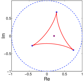
Abbildung 1: (Colour online) The $C$-numerical range for $A,C$ of Example 1.8 using the Lagrange-type gradient-flow algorithm [7] described in the text. The dots give the $C$-spectrum of $A$, where the interior ones coincide with the star centre.

2 Local $C$-Numerical Ranges

In view of applications in quantum control, it is customary to term the $n$-fold tensor product $SU(2)\otimes SU(2)\otimes\cdots\otimes SU(2)$ as the group of local unitary operations $SU_{\rm loc}(2^{n})$. It is a subgroup to the full dynamic group $SU(2^{n})$. Consequently, to a given initial state $A$, the reachability set under local controls amounts to the local unitary orbit $\mathcal{O}_{\rm loc}(A):=\{KAK^{\dagger}|K\in SU_{\rm loc}(2^{n})\}$.

Definition 2.1.

As in the companion paper [1], we define as local $C$-numerical range of $A$ the subset

$$W_{\rm{loc}}(C,A):=\{\operatorname{tr}\,(C^{\dagger}KAK^{\dagger})\;|\;K\in SU_{\rm loc}(2^{n})\}\subseteq W(C,A).$$ (31)

It can be viewed as a projection of the local unitary orbit of the initial state $A$ onto the target state $C$.

As also seen in the concomitant study, in contrast to the usual $C$-numerical range, its local counterpart is no longer star-shaped, nor simply connected. With these stipulations, we will discuss recent applications of the local $C$-numerical range in quantum control.

2.1 Application in Quantum Information

Again, in terms of Euclidean geometry, maximising the real part in $W_{\rm loc}(C,A)$ minimises the distance from $C$ to the local unitary orbit $\mathcal{O}_{\rm loc}(A)$.

In Quantum Information Theory, the minimal distance has an interesting interpretation in the following setting: let $A$ be an arbitrary rank-$1$ state of the form $A=|\psi\rangle\langle\psi|{}$ and let $C=\operatorname{diag}{}(1,0,\dots,0)\in\operatorname{Mat}{}_{2^{n}}(\mathbb{C}^{\,}{})$. Thus in this case $W_{\rm loc}(C,A)$ reduces to what we define as the local field of values ${W_{\rm loc}(A)}$.

Definition 2.2 ((Pure-State Entanglement)).

An $n$-qubit pure state $A=|\psi\rangle\langle\psi|{}$ with $|\psi\rangle{}\in\mathbb{C}^{\,2^{n}}{}$ is termed a product state, if it can be written as a tensor product

$$A=|\psi_{1}\rangle\langle\psi_{1}|{}\otimes|\psi_{2}\rangle\langle\psi_{2}|{}\otimes\cdots\otimes|\psi_{n}\rangle\langle\psi_{n}|{}\quad\text{with}\quad|\psi_{j}\rangle{}\in\mathbb{C}^{\,2}{}\quad,$$ (32)

whereas it is said to be entangled if it cannot.

In the present context, there are important observations with regard to the full unitary orbit $\mathcal{O}_{u}(A)$ and the local unitary orbit $\mathcal{O}_{\rm loc}(A)$ of pure states $A$ of different types:

1. all pure states form an equivalence class coinciding with $\mathcal{O}_{u}(A)$ if $A=|\psi\rangle\langle\psi|{}$ is an arbitrary pure state;

2. generic elements on the full unitary orbit $\mathcal{O}_{u}(A)$ of a pure product state $A$ are pure, yet no longer of product form;

3. all pure product states form an equivalence class coinciding with the local unitary orbit $\mathcal{O}_{\rm loc}(A)$ of an arbitrary pure product state $A$.
   

Consequently, measures of entanglement remain invariant under local unitary transformation.

Corollary 2.3 ((Euclidean Measure of Pure-State Entanglement)).

For $A=|\psi\rangle\langle\psi|{}$, $C=\operatorname{diag}{}(1,0,\dots,0)\in\operatorname{Mat}{}_{2^{n}}(\mathbb{C}^{\,}{})$ the minimial Euclidean distance

$$\Delta:=\underset{K\in SU_{\rm loc}(2^{n})}{\min}\;||KAK^{\dagger}-C||_{2}$$ (33)

is a measure of pure-state entanglement because it quantifies how far $A$ is from the equivalence class of pure product states. It relates to the maximum real part of the local numerical range $W_{\rm loc}(A)$ via

$$\begin{split}{||C-KAK^{\dagger}||}_{2}^{2}&={||A||}_{2}^{2}+{||C||}_{2}^{2}-2\operatorname{Re}\operatorname{tr}\{C^{\dagger}\;KAK^{\dagger}\}\\ &=2-2\operatorname{Re}\operatorname{tr}\{C^{\dagger}\;KAK^{\dagger}\}\quad,\end{split}$$ (34)

where the last equality holds if also $A$ is normalised to $||A||_{2}=1$.

The (squared) Euclidean distance from the nearest pure product state is illustrated in Fig. 2 for the following two examples taken from quantum information theory [36, 37]:

Example 2.4.

First, consider the pure 3-qubit state $A(s):=|\psi_{3}(s)\rangle\langle\psi_{3}(s)|{}$ parameterised by $0\leq s\leq 1$

$$|\psi_{3}(s)\rangle:=\sqrt{s}|W\rangle+\sqrt{1-s}|\tilde{W}\rangle\quad,$$ (35)

where  $|W\rangle{}:=\tfrac{1}{\sqrt{3}}{(0,1,1,0,1,0,0,0)^{t}}\quad{\rm and}\quad|\tilde{W}\rangle{}:=\tfrac{1}{\sqrt{3}}{(0,0,0,1,0,1,1,0)^{t}}$ .

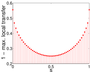
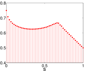
Abbildung 2: Euclidean distances of the pure states of Example 2.4 (a) and Example 2.5 (b) to the nearest pure product state as a function of $s$; here ‘max. local transfer’ denotes $\operatorname{Re}\operatorname{tr}\{C^{\dagger}\;KAK^{\dagger}\}$.

Example 2.5.

Likewise, observe the pure 4-qubit-state $A(s):=|\psi_{4}(s)\rangle\langle\psi_{4}(s)|{}$

$$|\psi_{4}(s)\rangle{}:=\sqrt{s}|GHZ^{\prime}\rangle{}-\sqrt{1-s}|\psi^{+}\rangle{}\otimes|\psi^{+}\rangle{}\quad,$$ (36)

where $|\rm GHZ^{\prime}\rangle{}:=\tfrac{1}{\sqrt{2}}{(0,0,0,1,0,0,0,0,0,0,0,0,1,0,0,0)^{t}}$ and
$|\psi^{+}\rangle{}\otimes|\psi^{+}\rangle{}:=\tfrac{1}{2}{(0,0,0,0,0,1,1,0,0,1,1,0,0,0,0,0)^{t}}$ .

Note that the plots in Fig. 2 quantitatively reproduce the global optimisation results found by numerical quadratic programming methods [36] yet cutting the cpu time by a factor of approx. $35$ in Example 2.4 and by a factor of some $150$ in Example 2.5. Moreover, in both cases, the findings coincide with the exact solutions known algebraically [37].

Caveat: in non-pure states, the problem of entanglement is much more involved, since the state space to non-pure states forms no simplex: a generic density operator has infinitely many decompositions into pure states. For recent overviews, see, e.g., ref. [38, 39]. Hence in those instances the above approach no longer applies.

2.1.1 Significance of Entanglement

Finally, it is the purpose of this tutorial paragraph to show the numerical-range focussed reader why in entangled quantum systems, the total system comprises more information than accessible from putting together the information of all its local subsystems.

To this end, we want to express a bipartite system $(a,b)$ in terms of its subsystems $a$ and $b$ by making use of the respective orthonormal Hilbert space vectors $|a_{\nu}\rangle{}\in\mathcal{H}{}_{a}$ and $|b_{\mu}\rangle{}\in\mathcal{H}{}_{b}$. For simple demonstration, we assume both to be of the same dimension and consider a type of density operator in the total Hilbert space $\mathcal{H}_{a}\otimes\mathcal{H}_{b}$ that can be expanded in the Schmidt bases as

$$\rho_{ab}=\sum_{\mu\nu}\lambda_{\mu\nu}(|a_{\mu}\rangle\langle a_{\nu}|{}\otimes|b_{\mu}\rangle\langle b_{\nu}|{})\quad.$$ (37)

The information locally accessible in subsystem $a$ is encoded in the reduced density operator of subsystem $a$ that is projected out by taking the so-called partial trace $\operatorname{tr}(|b_{\mu}\rangle\langle b_{\nu}|{})$ over the degrees of freedom of subsystem $b$ yielding

$$\begin{split}\rho_{a}:=\operatorname{tr}_{b}\{\rho_{ab}\}&=\operatorname{tr}_{b}\{\Sigma_{\mu\nu}\lambda_{\mu\nu}(|a_{\mu}\rangle\langle a_{\nu}|{}\otimes|b_{\mu}\rangle\langle b_{\nu}|{})\}\\ &=\Sigma_{\mu\nu}\lambda_{\mu\nu}(|a_{\mu}\rangle\langle a_{\nu}|{}\cdot\operatorname{tr}\{|b_{\mu}\rangle\langle b_{\nu}|{}\})\\ &=\Sigma_{\mu\nu}\lambda_{\mu\nu}(|a_{\mu}\rangle\langle a_{\nu}|{}\cdot{\langle b_{\nu}|b_{\mu}\rangle{}})\\ &=\Sigma_{\mu}\lambda_{\mu\mu}|a_{\mu}\rangle\langle a_{\mu}|{}\quad,\end{split}$$ (38)

where the last equality holds, because in the orthonormal Schmidt basis $\langle b_{\nu}|b_{\mu}\rangle{}=\delta_{\mu\nu}$. The following standard examples [40] will illustrate reduced states in the scenarios of product states on one hand, and entangled states on the other.

Example 2.6.

Product states take the form $\rho_{ab}=\rho_{a}\otimes\rho_{b}$, so one trivially finds

$$\rho_{a}=\operatorname{tr}_{b}\{\rho_{a}\otimes\rho_{b}\}=\rho_{a}\cdot\operatorname{tr}\rho_{b}=\rho_{a}$$ (39)

since $\operatorname{tr}\rho_{b}=1$ by definition of a normalised density operator.

Example 2.7.

However, in the Bell state $|\Phi\rangle{}:=\tfrac{1}{\sqrt{2}}(|00\rangle{}+|11\rangle{})$, where it is customary to use the short-hand $|0\rangle{}:=\left(\begin{smallmatrix}1\\ 0\end{smallmatrix}\right)\in\mathbb{C}^{\,2}{}$ and $|1\rangle{}:=\left(\begin{smallmatrix}0\\ 1\end{smallmatrix}\right)$ as well as $|00\rangle{}:=|0\rangle{}\otimes|0\rangle{}\in\mathbb{C}^{\,4}{}$ and likewise $|11\rangle{}:=|1\rangle{}\otimes|1\rangle{}$, one obtains

$$\begin{split}\rho_{ab}&=|\Phi\rangle\langle\Phi|{}=\tfrac{1}{2}(|00\rangle{}+|11\rangle{})(\langle 00|{}+\langle 11|{})\\[5.69054pt] \rho_{a}&=\operatorname{tr}_{b}|\Phi\rangle\langle\Phi|{}\\ &=\tfrac{1}{2}\operatorname{tr}_{b}\big{(}|00\rangle\langle 00|{}+|00\rangle\langle 11|{}+|11\rangle\langle 00|{}+|11\rangle\langle 11|{}\big{)}\\ &=\tfrac{1}{2}\big{(}|0\rangle\langle 0|{}_{a}{\langle 0|0\rangle{}_{b}}+|0\rangle\langle 1|{}_{a}{\langle 1|0\rangle{}_{b}}+|1\rangle\langle 0|{}_{a}{\langle 0|1\rangle{}_{b}}+|1\rangle\langle 1|{}_{a}{\langle 1|1\rangle{}_{b}}\big{)}\\ &=\tfrac{1}{2}\big{(}|0\rangle\langle 0|{}_{a}+|1\rangle\langle 1|{}_{a}\big{)}\\ &=\tfrac{1}{2}{\rm 1\negthickspace l}{}_{a}\\[5.69054pt] \rho_{b}&=\operatorname{tr}_{a}|\Phi\rangle\langle\Phi|{}=\tfrac{1}{2}{\rm 1\negthickspace l}{}_{b}\end{split}$$ (40)

The second example shows the generic situation: although $\rho_{ab}$ is a pure state, the reduced states of the respective subsystems $\rho_{a(b)}\in\mathcal{H}{}_{a(b)}$ are no longer pure.

Compare the information content:

1. $\rho_{ab}^{\phantom{2}}=\rho_{ab}^{2}$ contains all information about the total system;

2. $\rho_{a(b)}$ contains all information about the respective subsystem $a(b)$;

3. the reconstruction $\rho_{ab}^{\prime}:=\rho_{a}\otimes\rho_{b}\neq\rho_{ab}^{\prime 2}$ puts together all information accessible from both local subsystems; this is generically less than in $\rho_{ab}$.
   

In the second example, the reconstruction $\rho_{ab}^{\prime}=\rho_{a}\otimes\rho_{b}=\tfrac{1}{4}{\rm 1\negthickspace l}{}$ is diagonal, whereas the original $\rho_{ab}=\sum_{\mu\nu}\lambda_{\mu\nu}(|a_{\mu}\rangle\langle a_{\nu}|{}\otimes|b_{\mu}\rangle\langle b_{\nu}|{})$ contained off-diagonal terms. Thus it is the coherent phase relation between the local constituents that is inevitably lost upon projection to the respective reduced systems. It cannot be reconstructed a posteriori using but local pieces of information. This shows how in entangled quantum systems, the total system comprises more information than is accessible from putting together the information of all its reduced local subsystems. Measures of entanglement account for this loss of information and thus play an important role in quantum information theory.

2.2 Application in Quantum Simulation

In quantum control, it is of interest to decide, whether a given multi-particle quantum interaction (expressed by some interaction Hamiltonian $H$) can be sign-reversed solely by local unitary operations. If this is the case, one may undo or refocus the time evolution of such an interaction purely by local operations generalising the sense of the celebrated Hahn spin echo [41, 42] in the following way: (0) start with any initial sate, (1) let the interaction evolve for some time $t$ to give the propagator $e^{-itH}$, (2) apply appropriate local operations, (3) let the interaction evolve again for the same duration $t$, (4) apply the inverse to the previous local operations to (5) recover the initial state again as an echo, because steps (2)–(3)–(4) bring about the inverse propagator $e^{+itH}$. Note the same local operations apply to all the initial states; they only depend on the interaction Hamiltonian $H$.

Mathematically, we ask whether there is a $K\in SU_{\rm loc}(2^{n})$ such that

$$K\;e^{-itH}\;K^{\dagger}=e^{+itH}\quad\mbox{for all}\;t\in\mathbb{R}^{\,+}{}\quad.$$ (41)

Due to the equality $K\;e^{-itH}\;K^{\dagger}=e^{-itKHK^{\dagger}}$ the question readily boils down to deciding whether the sign-reversed Hamiltonian $-H$ is on the local unitary orbit of the original Hamiltonian $H$, i.e., does there exist $K\in SU_{\rm loc}(2^{n})$ such that

$$K\;H\;K^{\dagger}=-H\quad.$$ (42)

Recently, we have solved this problem based on its normal form [43]: this is sign reversibility by local $z$-rotations, since every element $K\in SU_{\rm loc}(2^{n})$ is locally unitarily similar to local $z$-rotations. Here, we focus on the relation to local $C$-numerical ranges by illustrating that normalised Hamiltonians $H$ are sign-reversible if and only if $W_{\rm loc}(H,H)=[-1;+1]$, cf. [43]. To this end, define the spin-$\tfrac{1}{2}$ operators

$$J_{0}:={\rm 1\negthickspace l}{}_{2}\;;\quad J_{z}:=\tfrac{1}{2}\operatorname{diag}{}(1,-1)\;;\quad J_{+}:=\left(\begin{smallmatrix}0&1\\ 0&0\end{smallmatrix}\right)\;;\quad J_{-}:=J_{+}^{\dagger}=\left(\begin{smallmatrix}0&0\\ 1&0\end{smallmatrix}\right)\;.$$ (43)

In a single qubit, the $J_{\nu}\in\{J_{0},J_{z},J_{+},J_{-}\}$ are the eigenoperators to the conjugation map $\operatorname{Ad_{e^{-i\phi J_{z}}}}$, i.e.

$$\operatorname{Ad_{e^{-i\phi J_{z}}}}(J_{\nu}):=e^{-i\phi J_{z}}\;J_{\nu}\;e^{+i\phi J_{z}}=e^{-ip_{\nu}\phi}\;J_{\nu}$$ (44)

associated with the respective eigenvalues $e^{-ip_{\nu}\phi}$, $p_{0}=p_{z}=0$ and $p_{\pm}=\pm 1$. In order to generalise the arguments to the case of $z$-rotations on $n$ qubits with individually differing rotation angles on each spin qubit $\phi_{1},\phi_{2},\dots,\phi_{\ell},\dots,\phi_{n}$, we write

$$K_{z}(\phi_{1},\;\dots\;,\phi_{n})=e^{-i\phi_{1}J_{z}}\otimes e^{-i\phi_{2}J_{z}}\otimes\dots\otimes e^{-i\phi_{n}J_{z}}\in{SU}_{\rm loc}(2^{n}).$$ (45)

Now consider a Hamiltonian in normal form $\bar{H}$ taking the special form $\bar{H}:=\bar{H}_{+}+\bar{H}_{-}$ with $\bar{H}_{-}:=\bar{H}_{+}^{\dagger}$, where $\bar{H}_{+}$ is a tensor product of $\operatorname{Ad_{e^{-i\phi J_{z}}}}$ eigenoperators on each spin qubit $\ell=1,\dots,n$ according to

$$\bar{H}_{+}:=J_{\nu_{1}}^{(1)}{}\otimes J_{\nu_{2}}^{(2)}{}\otimes\cdots\otimes J_{\nu_{\ell}}^{(\ell)}{}\otimes\cdots\otimes J_{\nu_{n}}^{(n)}{}$$ (46)

with independent $\nu_{\ell}\in\{0,z,+,-\}$ on each spin qubit. With $\bar{H}_{\pm}$ satisfying

$$\operatorname{Ad_{K_{z}(\phi_{1},\;\dots\;,\phi_{n})}}\big{(}\bar{H}_{\pm}\big{)}=e^{\mp i(p_{\nu_{1}}\phi_{1}+\;\cdots\;+p_{\nu_{n}}\phi_{n})}\;\bar{H}_{\pm}\;,$$ (47)

the Hamiltonian $\bar{H}$ is sign-reversed by local $z$-rotations provided there exists a set of rotation angles $\{\phi_{\ell}\}$ satisfying $\sum_{\ell=1}^{n}p_{\nu_{\ell}}\phi_{\ell}=\pm\pi\;(\operatorname{mod}2\pi)\;.$ This is the case if there is at least one spin qubit $\ell$ giving rise to an interaction of quantum order $p_{\nu_{\ell}}=\pm 1$.

Moreover, a (real) linear combination

$$\bar{H}_{\Sigma}:=\sum_{\lambda=1}^{m}c_{\lambda}\bar{H}_{\lambda}$$ (48)

of Hamiltonians $\bar{H}_{\lambda}:=\bar{H}_{\lambda+}+\bar{H}_{\lambda-}$ with $\bar{H}_{\lambda+}$ as in Eqn. 46 is jointly reversible by individual local $z$-rotations $K_{z}(\phi_{1},\;\dots\;,\phi_{n})$ , if there is at least one consistent set of rotation angles $\{\phi_{\ell}\}$ simultaneously fulfilling a standard linear system of $m$ equations in $n$ variables

$$\begin{pmatrix}p_{1\nu_{1}}&p_{1\nu_{2}}&\cdots&p_{1\nu_{n}}\\ p_{2\nu_{1}}&p_{2\nu_{2}}&\cdots&p_{2\nu_{n}}\\ p_{3\nu_{1}}&p_{3\nu_{2}}&\cdots&p_{3\nu_{n}}\\ \vdots&\vdots&\ddots&\vdots\\ p_{m\nu_{1}}&p_{m\nu_{2}}&\cdots&p_{m\nu_{n}}\\ \end{pmatrix}\begin{pmatrix}\phi_{1}\\ \phi_{2}\\ \vdots\\ \phi_{n}\end{pmatrix}=\begin{pmatrix}\pi\;(\operatorname{mod}2\pi)\\ \pi\;(\operatorname{mod}2\pi)\\ \pi\;(\operatorname{mod}2\pi)\\ \vdots\\ \pi\;(\operatorname{mod}2\pi)\end{pmatrix}.$$ (49)

With these stipulations, we have recently proven the following interrelations in view of local $C$-numerical ranges:

Corollary 2.8 ((Local Time Reversal [43])).

For $H=H^{\dagger}$ with $\|H\|{}_{2}^{\phantom{2}}=1$ the following are equivalent:

1. the Hamiltonian $H$ is sign-reversible under local unitary operations;

2. its local $C$-numerical range comprises $-1$, i.e., $-1\in W_{\rm loc}(H,H)$;

3. its local $C$-numerical range is the interval $[-1\,;\,+1]\;=\;W_{\rm loc}(H,H)$;

4. there exists a $K\in SU_{\rm loc}(2^{n})$ such that $\operatorname{Ad}_{K}(H)=-H$;

5. $H$ is locally unitarily similar to a $\bar{H\;}$ with $\operatorname{Ad}_{K_{z}(\phi_{1},\dots,\phi_{n})}(\bar{H\;})=-\bar{H\;}$;

6. $H$ is locally unitarily similar to a linear combination of the form Eqn. 48 satisfying the system of linear equations given in Eqn. 49;

7. let $\mathfrak{g}=\mathfrak{g}_{0}\oplus\;\bigoplus\limits_{i\neq j}\mathbb{C}^{\,}{}E_{ij}$ be the root-space decomposition of $\mathfrak{sl}(N,\mathbb{C}^{\,}{})$, where $E_{ij}$ denotes the square matrix differing from the zero matrix by just one element, the unity in the $j^{\rm th}$ column of the $i^{\rm th}$ row; then $H$ is locally unitarily similar to a linear combination of root-space elements to non-zero roots (so $i\neq j$) with $\bar{H}_{\Sigma}\,:=\sum_{\lambda=1}^{m}c_{\lambda}E_{ij}^{(\lambda)}$ satisfying the system of linear equations $\sum_{\ell=1}^{n}p_{\lambda,\ell}\cdot\phi_{\ell}=\pi(\operatorname{mod}2\pi)$ for $\lambda=1,2,\dots,m$ as in Eqn. 49.

In ref. [43], we provided more tools to assess local reversibility by means of eigenspaces, graph representations of the interaction topology, spherical tensor methods, and root-space decomposition. Based on assertion (4) we also implemented a gradient-flow algorithm on the group of local unitaries $SU_{\rm loc}(2^{n})$ in order to tackle the problem numerically.

In the accompanying paper, we show the following:

Theorem 2.9 ((Local $C$-Numerical Ranges of Circular Disc Shape [1])).

Let $\mathbf{K}$ be a compact connected subgroup of $U(N)$ with Lie algebra $\mathfrak{k}$, and let $\mathfrak{t}$ be a torus algebra of $\mathfrak{k}$. Then the relative $C$-numerical range $W_{\mathbf{K}}(C,A_{+})$ of a matrix $A_{+}\in\operatorname{Mat}{}_{N}(\mathbb{C}^{\,}{})\setminus 0$ is a circular disc centered at the origin of the complex plane for all $C\in\operatorname{Mat}{}_{N}(\mathbb{C}^{\,}{})$ if and only if there exists a $K\in\mathbf{K}$ and a $\Delta\in\mathfrak{t}$ such that $KA_{+}K^{\dagger}$ is an eigenoperator to $\operatorname{ad}_{\Delta}$ with a non-zero eigenvalue

$$\operatorname{ad}_{\Delta}(KA_{+}K^{\dagger})\equiv[\Delta,KA_{+}K^{\dagger}]=ip\;KA_{+}K^{\dagger}\quad\text{\rm and}\quad p\neq 0\quad.$$ (50)

Clearly, if $KA_{+}K^{\dagger}$ is an eigenoperator of $\operatorname{ad}_{\Delta}$ to the eigenvalue $+ip$ and $A_{-}:=A_{+}^{\dagger}$, then $KA_{-}K^{\dagger}$ shows the eigenvalue $-ip$. $A_{+}$ and $A_{-}$ share the same relative $C$-numerical range of circular symmetry, $W_{K}(C,A_{+})=W_{K}(C,A_{-})$.

Moreover, locally reversible Hamiltonians $H$ and nilpotent matrices $\{A_{+},A_{-}\}$ with rotationally symmetric local $C$-numerical ranges are related as follows:

Corollary 2.10.

Let $\mathbf{K}=SU_{\rm loc}(2^{n})$. Let $A_{+}$ and $A_{-}:=A_{+}^{\dagger}$ both share the same local $C$-numerical ranges $W_{\rm loc}(C,A_{\pm})$ of circular disc shape for all $C$.
Then

1. any linear combination $A_{\lambda}:=A_{+}+\lambda A_{-}$ with $\lambda\in\mathbb{C}^{\,}{}$ and in particular the Hermitian $H:=A_{+}+A_{-}$ are sign reversible by some local $K\in SU_{\rm loc}(2^{n})$, so $W_{\rm loc}(H,H)=[-||A||_{2}^{2};+||A||_{2}^{2}]$, whereas

2. the converse does not necessarily hold: there are locally reversible Hermitian $H$ to which no decomposition into a single pair $\{H_{+},H_{-}\}$ sharing the same rotationally symmetric local $C$-numerical range $W_{\rm loc}(C,H_{\pm})$ exist, but

3. every Hermitian $H\in\operatorname{Mat}{}_{2^{n}}(\mathbb{C}^{\,}{})$ that is locally sign reversible can be decomposed into at most ${2^{n}}\choose{2}$ pairs $(H^{(1)}_{+},H^{(1)}_{-}),(H^{(2)}_{+},H^{(2)}_{-}),\dots$ with each pair sharing the same rotationally symmetric local $C$-numerical range $W_{\rm loc}(C,H^{(\ell)}_{\pm})$.

Proof 2.11.

:

1. Eqn. 50 is equivalent to

   $$\begin{split}\operatorname{Ad}_{e^{-\phi\Delta}}(KA_{+}K^{\dagger})&\equiv e^{-\phi\Delta}(KA_{+}K^{\dagger})e^{+\phi\Delta}\\ &=e^{-\phi\operatorname{ad}_{\Delta}}(KA_{+}K^{\dagger})=e^{-i\phi p}KA_{+}K^{\dagger}\quad,\vspace{-9mm}\end{split}$$ (51)

   thus $p\neq 0$ ensures a $\phi$ with $e^{\pm i\phi p}=-1$ to sign-reverse both $KA_{\pm}K^{\dagger}$.

2. By Corollary 2.8, local sign-reversibility allows for linear combinations of eigenoperators to different $\operatorname{ad}_{\Delta}$-operators with different eigenvalues thus generically violating the conditions for rotational symmetry of Theorem 2.9.

3. By Corollary 2.8 any Hermitian $\bar{H}\in\operatorname{Mat}{}_{2^{n}}(\mathbb{C}^{\,}{})$ locally reversible by $z$-rotations can trivially be decomposed into at most $2^{n}\choose 2$ Hermitian components $(\lambda_{ij}E_{ij}+\lambda_{ij}^{*}E_{ji})$ with $1\leq i<j\leq N=2^{n}$ and $\lambda_{ij}\in\mathbb{C}^{\,}{}$, where the $(\bar{H}_{+}^{(\ell)},\bar{H}_{-}^{(\ell)}):=(\lambda_{ij}E_{ij},\lambda_{ij}^{*}E_{ji})$ share the same rotationally symmetric local $C$-numerical range.

3 Constrained Optimisation and Relative $C$-Numerical Ranges

In quantum control, one may face the problem to maximise the unitary transfer from matrices from $A$ to $C$ subject to suppressing the transfer from $A$ to $D$, or subject to leaving another state $E$ invariant. For tackling those types of problems, in ref. [7] we introduced a ‘constrained $C$-numerical range of $A$’.

Definition 3.1.

The constrained $C$-numerical range of $A$ is defined by

$$W(C,A)\big{|}_{\rm constraint}\,:=\,\big{\{}\operatorname{tr}(UAU^{\dagger}{}C^{\dagger}{})\,\big{|}\;\text{constraint}\big{\}}\subseteq W(C,A)\;.$$ (52)

In ref. [7] we also asked which form it takes and—in view of numerical optimisation—whether it is a connected set with a well-defined boundary. Connectedness is central to any numerical optimisation approach, because otherwise one would have to rely on initial conditions in the connected component of the (global) optimum.

Exploiting the findings on the relative $C$-numerical range of the accompanying paper [1], the structure of constrained $C$-numerical ranges can readily be characterised in some simple cases.

Corollary 3.2.

The constrained $C$-numerical range of $A$ is a connected set in the complex plane, if the constraint can be fulfilled by restricting the full unitary group $U(N)$ to a compact and connected subgroup $\mathbf{K}\subseteq U(N)$.

In this case, the constrained $C$-numerical range $W(C,A)|_{\rm constraint}$ is identical to the relative $C$-numerical range $W_{\mathbf{K}}(C,A)$ and hence the constrained optimisation problem is solved within it, e.g., by the corresponding relative $C$-numerical radius $r_{\mathbf{K}}(C,A)$ .

Proof 3.3.

: Direct consequence of the properties of the relative $C$-numerical range $W_{\mathbf{K}}(C,A)$ introduced in the accompanying paper [1]: if $\mathbf{K}$ is compact and connected, then $W_{\mathbf{K}}(C,A)$ is so as well, since it is a continuous image of a compact and connected set.

Note that although being connected, $W_{\mathbf{K}}(C,A)$ is in general neither star-shaped nor simply connected [1]. So if $\mathbf{K}$ is compact and connected this obviously extends to $W(C,A)|_{\rm constraint}$.

3.0.1 Constraint by Invariance

The problem of maximising the transfer from $A$ to $C$ while leaving $E$ invariant

$$\underset{U}{\max}|\operatorname{tr}\{UAU^{\dagger}{}C^{\dagger}{}\}|\quad\text{\rm subject to}\quad UEU^{\dagger}{}=E$$ (53)

is straightforward in as much as the stabiliser group of $E$

$$\mathbf{K}_{E}:=\{K\in U(N)\,|\,KEK^{\dagger}=E\}$$ (54)

is easy to come by: it is generated by the Lie-algebra elements

$$\mathfrak{k}_{E}:=\{k\in\mathfrak{u}(N)\,|\,\operatorname{ad}_{k}(E)\equiv[k,E]=0\}\quad.$$ (55)

In particular, if $E$ is of the form $E=\mu{\rm 1\negthickspace l}{}+\Omega$ with $\mu\in\mathbb{C}^{\,}{}$ and $\Omega\in\mathfrak{u}(N)$, then $\mathfrak{k}_{E}$ is identical to the centraliser of $\Omega$ in $\mathfrak{u}(N)$.

Lemma 3.4.

The set $\mathfrak{k}_{E}$ is closed under the Lie bracket, hence it is a subalgebra to $\mathfrak{u}(N)$ thus generating a subgroup $\mathbf{K}_{E}\subseteq U(N)$, to wit the stabiliser group.

Proof 3.5.

: Direct consequence of the Jacobi identity for the double commutator: $[[A,B],E]+[[B,E],A]+[[E,A],B]=0$ for all $A,B,E\in\operatorname{Mat}{}_{N}(\mathbb{C}^{\,}{})$. Hence $[k_{1},E]=[k_{2},E]=0$ implies $[[k_{1},k_{2}],E]=0$ and $\mathfrak{k}_{E}$ is a Lie subalgebra to $\mathfrak{u}(N)$ thus generating a compact connected stabiliser group $\mathbf{K}_{E}\subseteq U(N)$.

The stabiliser group of any $E\in\operatorname{Mat}{}_{N}(\mathbb{C}^{\,}{})$ in $U(N)$ is connected. This is in general not the case in $SU(N)$ as easily seen for $E:=\left(\begin{smallmatrix}0&1\\ 0&0\end{smallmatrix}\right)$. However, one can restrict the above optimisation to the connected component of the identity matrix in SU(N) due to the invariance properties of the function $U\mapsto\operatorname{tr}\{UAU^{\dagger}{}C^{\dagger}{}\}$.

A set of generators of $\mathfrak{k}_{E}$ may constructively be found via the kernel of the commutator map by solving a homogeneous linear system

$$\mathfrak{k}_{E}=\ker\operatorname{ad}_{E}\cap\,\mathfrak{su}(N)=\{k\in\mathfrak{su}(N)|({\rm 1\negthickspace l}{}\otimes E-E^{t}\otimes{\rm 1\negthickspace l}{})\operatorname{vec}(k)=0\}\quad.$$ (56)

Corollary 3.6.

If solvable in an non-trivial way, the optimisation problem of Eqn. 53 entails a constrained $C$-numerical range that is connected. Moreover, it takes the form of a relative $C$-numerical range

$$W(C,A)\big{|}_{\operatorname{Ad}_{U}(E)=E}:=\{\operatorname{tr}(UAU^{\dagger}{}C^{\dagger}{})\,|\,UEU^{\dagger}{}=E\}=W_{\mathbf{K}_{E}}(C,A)\quad$$ (57)

and the optimisation problem is solved by the relative $C$-numerical radius $r_{\mathbf{K}_{E}}(C,A)$. In Hermitian $E$, $\mathbf{K}_{E}$ includes a maximal torus group $\mathbf{T}\subset SU(N)$.

Proof 3.7.

: To any $E\in\operatorname{Mat}{}_{N}(\mathbb{C}^{\,}{})$ the existence of a compact connected stabiliser group $\mathbf{K}_{E}\subset U(N)$ can constructively be checked as in Eqn. 56. Moreover, every Hermitian $E$ can be chosen diagonal; hence in that case $\mathfrak{k}_{E}$ includes a maximal torus algebra $\mathfrak{t}$ with $\mathfrak{t}\subset\mathfrak{k}_{E}\subset\mathfrak{u}(N)$. The rest follows.

Obviously, the constraint of leaving $E$ invariant while maximising the transfer from $A$ to $C$ only makes sense, if $A$ and $E$ do not share the same stabiliser group.

Since it may be tedious to check for the stabiliser group $\mathbf{K}_{E}$ of $E$ in each and every practical instance and then project the gradients onto the corresponding subalgebra $\mathfrak{k}_{E}$, a more versatile programming tool would be welcome.

To this type of constrained optimisation, in ref. [7], we also derived a gradient flow based on the Lagrange function (with $f_{C}(U):=\operatorname{tr}\{C^{\dagger}UAU^{\dagger}\}$)

$$L(U)=|f_{C}(U){}|{}^{2}-\lambda\left(\operatorname{tr}\{UEU^{\dagger}{}E^{\dagger}{}\}-||E||_{2}^{2}\right)\quad,$$ (58)

where the constraint $UEU^{\dagger}{}-E=0$ was written in the more convenient form $\operatorname{tr}\{UEU^{\dagger}{}E^{\dagger}{}\}-\|E\|{}_{2}^{2}=0$. The algorithm implements the gradient from the Fréchet derivatives

$$\begin{split}D\,\big{\{}|f_{C}(U){}|{}^{2}&-\lambda f_{E}(U){}+\lambda\,\|E\|{}_{2}^{2}\big{\}}\,(iHU)\\ &=\operatorname{tr}\big{\{}\,\big{(}2\,(f_{C}^{*}(U){}[UAU^{\dagger},C^{\dagger}]{})_{S}-\lambda[UEU^{\dagger},E^{\dagger}]{}\big{)}\,iH\big{\}}\quad,\end{split}$$ (59)

where for short, $(\cdot)_{S}$ denotes the skew-Hermitian part, within the recursion [7]

$$U_{k+1}=\exp\big{\{}-\alpha\,\big{(}2\,(f_{C}^{*}(U_{k}){}[U_{k}^{\phantom{\dagger}}AU_{k}^{\dagger},C_{\phantom{k}}^{\dagger}]{})_{S}-\lambda[U_{k}^{\phantom{\dagger}}EU_{k}^{\dagger},E^{\dagger}]{}\big{)}\,\big{\}}\,U_{k}\quad.$$ (60)

3.0.2 Constraint by Orthogonality

For the sequel of this paragraph, we assume a generic shape of the $C$-numerical range $W(D,A)$ so that $m_{0}\in W(D,A)$ defines the unique point in $W(D,A)$ that is closest to the origin in the complex plane. For these instances, we address the optimisation problem

$$\underset{U}{\max}|\operatorname{tr}\{UAU^{\dagger}{}C^{\dagger}{}\}|\quad\text{\rm subject to}\quad\operatorname{tr}\{UAU^{\dagger}{}D^{\dagger}{}\}=m_{0}\quad.$$ (61)

Clearly, perfect matches exist if $0\in W(D,A)$, because only then are there points on the unitary orbit $\mathcal{O}_{u}(A)$ that are orthogonal to $D$. Moreover by Eqn. 7, the modulus of $m_{0}$ relates to the cosine of the angle between $D$ and points on the unitary orbit $\mathcal{O}_{u}(A)$ that come closest to orthogonality. The corresponding $C$-numerical range constrained by (best approximation to) orthogonality to $D$ takes the form [7]

$$W(C,A)\big{|}_{\operatorname{Ad}_{U}\perp D}\,:=\,\big{\{}\operatorname{tr}\{UAU^{\dagger}{}C^{\dagger}{}\}\,\big{|}\;|\operatorname{tr}\{UAU^{\dagger}{}D^{\dagger}{}\}|\,=\,m_{0}\big{\}}\subseteq W(C,A)\;,$$ (62)

which is more difficult to characterise, because in order to establish whether it is a connected set in the complex plane, one has to check the constraint set

$$\tilde{K}_{D}\,:=\,\{K\subseteq SU(N)\,|\,\operatorname{tr}\{KAK^{\dagger}D^{\dagger}{}\}=m_{0}\;\}$$ (63)

for its properties of (i) forming a subgroup and (ii) connectedness. Generically, already the first condition is violated, and only in the rare event of both of them being fulfilled, the set $\tilde{K}_{D}$ turns into a subgroup ${\mathbf{K}}_{D}$, and hence the constrained $C$-numerical range into the relative $C$-numerical range $W_{{\mathbf{K}}_{D}}(C,A)$. Then the constrained optimisation problem of Eqn. 61 would be solved by the relative $C$-numerical radius $r_{{\mathbf{K}}_{D}}(C,A)$. Even in the special case $m_{0}\,=\,0\in W(D,A)$ it is difficult to make sure the projection of the unitary orbit $\mathcal{O}_{u}(A)$ onto the orthocomplement $D^{\perp}$ of $D$ in the Hilbert space $(\operatorname{Mat}{}_{N}(\mathbb{C}^{\,}{}),\operatorname{tr}\{\cdot^{\dagger}\cdot\})$ is still a smooth manifold. Generically, again this is not the case.

It is for these reasons that addressing orthogonality problems by a Lagrange approach is more promising. For this to make sense, one trivially has to ensure $C$ and $D$ are not scalar multiples of one another, yet is not necessary that perfect orthogonality in the sense of $0\in W(D,A)$ can actually be achieved.

In ref. [7], we devised a Lagrange-type gradient-flow algorithm for solving the constrained optimisation problem of Eqn. 61 numerically. To this end, define $f_{C}(U){}:=\operatorname{tr}\{UAU^{\dagger}{}C^{\dagger}{}\}$ and $f_{D}(U){}:=\operatorname{tr}\{UAU^{\dagger}{}D^{\dagger}{}\}$. Introducing the Lagrange function

$$L(U):=|f_{C}(U){}|{}^{2}-\lambda\,|f_{D}(U){}|{}^{2}\quad,$$ (64)

the task to maximise the transfer from $A$ to $C$ while suppressing the transfer from $A$ to $D$ can be addressed by implementing the gradient of

$$\begin{split}D\big{\{}|f_{C}(U){}|{}^{2}-\lambda\,|f_{D}(U){}|{}^{2}\big{\}}\,(iHU)&\,=\\ \operatorname{tr}\,\big{\{}2\,(f_{C}^{*}(U){}[UAU^{\dagger},C^{\dagger}]{})_{S}\;iH\big{\}}&\,-\,\lambda\,\operatorname{tr}\,\big{\{}2\,(f_{D}^{*}(U){}[UAU^{\dagger},D^{\dagger}]{})_{S}\;iH\big{\}}\end{split}$$ (65)

into the recursive scheme [7]

$$U_{k+1}=\exp\{-2\alpha\,\big{(}(f_{C}^{*}(U_{k}){}[U_{k}^{\phantom{\dagger}}AU_{k}^{\dagger},C_{\phantom{k}}^{\dagger}]{})_{S}\,-\,\lambda\,\big{(}f_{D}^{*}(U_{k}){}[U_{k}^{\phantom{\dagger}}AU_{k}^{\dagger},D_{\phantom{k}}^{\dagger}]{}\big{)}_{S}\big{)}\}\,U_{k}\quad.$$ (66)

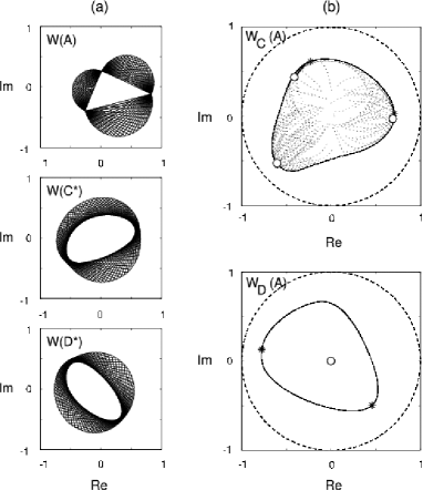
Abbildung 3: Constrained optimisation $A\to C$ suppressing $A\to D$ for matrices $A,C,D$ of Ex. 3.8.

Example 3.8.

In Fig. 3, a first example is given for the matrices

$$A = {\left(\begin{smallmatrix}\phantom{-}0.8359-0.1152i&0&0\\ 0&-0.2593-0.3906i&0\\ 0&0&\phantom{-}0.0151+0.2609i\end{smallmatrix}\right)}$$ (67)

$$C = {\left(\begin{smallmatrix}-0.0318+0.0690i&-0.3522-0.3185i&\phantom{-}0.2351-0.3050i\\ -0.0404+0.0656i&\phantom{-}0.0844-0.2880i&\phantom{-}0.2135+0.3234i\\ \phantom{-}0.3086+0.1076i&\phantom{-}0.1742-0.2291i&-0.2368+0.3585i\end{smallmatrix}\right)}$$ (68)

$$D = {\left(\begin{smallmatrix}-0.2910-0.3480i&-0.2395+0.0274i&-0.2428+0.0656i\\ \phantom{-}0.0836-0.2790i&-0.1836-0.0203i&-0.2427+0.2396i\\ -0.3906-0.1387i&\phantom{-}0.1989-0.2725i&-0.0442+0.3871i\end{smallmatrix}\right)}$$ (69)

the first one of which is normal thus entailing a triangular pattern in its numerical range $W(A)$ shown together with $W(C^{\dagger}{})$ and $W(D^{\dagger}{})$ in column (a). The conventional numerical ranges were calculated using the classical algorithm of Marcus [44, 45, 46]. By the constraint that the transfer from $A$ to $D$ be minimal, the local maxima on the boundary $\partial{W(C,A)}$ of the $C$-numerical range of $A$ (asterisks in column (b)) are shifted to the points indicated by noughts. Note that only the upper left one seems to be displaced from the boundary $\partial{W(C,A)}$ slightly into the interior of $W(C,A)$. All the 100 trajectories (shown as dotted lines) starting from random initial conditions converge into the same maxima, while the transfer from $A$ to $D$ gets zero as shown in the $C$-numerical range $W(D,A)$ at the bottom of column (b).

4 Conclusions

We have shown how $C$-numerical ranges provide the setting for many quantum optimisations. Knowing about its structure paves the way to numerical algorithms, e.g., for plotting its shape. In the accompanying paper, we introduced the relative $C$-numerical range of $A$ as a restriction of the full unitary group $U$ to some compact connected subgroup $\mathbf{K}\subset U$, in which case it is connected but not simply connected. Here we illustrated that this is of practical importance in relevant examples from quantum information: For instance, the maximum real part of the local $C$-numerical range of $A$ (as a special case of the relative $C$-numerical range) directly corresponds to a measure of ‘pure-state entanglement’. In other instances, if the local $C$-numerical range of a normalised interaction Hamiltonian $H$ is $W_{\rm loc}(H,H)=[-1,+1]$, then the interaction is locally reversible. These cases are fully characterised in Lie algebraic terms (by root-space elements to non-zero roots fulfilling a linear system of equations) and they are related to cases, where the local $C$-numerical range is a circular disc in the complex plane.

Moreover, some constrained optimisation problems in quantum control can be treated group theoretically: if the constraining conditions can be translated into restricting the full quantum dynamics on $U$ to a compact connected subgroup $\mathbf{K}$, then the optimisation problem remains within the corresponding connected relative $C$-numerical range and the optimisation amounts to finding its relative $C$-numerical radius. For more general cases we provide numerical algorithms for constrained optimisations of Lagrange-type.

5 Outlook

Motivated by applications in quantum control, the relative $C$-numerical range of $A$ introduced awaits further mathematical elucidation: for instance, what are the properties of its boundary, under which conditions is it simply connected, or even star-shaped? When is it convex? How can one systematically find compact connected subgroups embracing practical constraints of quantum optimisation so that they relate to a connected relative $C$-numerical range? What happens in generalisations where the subgroups are no longer compact and connected? Are there simple instances, in which the correponding restricted $C$-numerical ranges have few connected components and thus are not ‘hopeless’ in view of practical optimisation? Can one prove the conjecture of ref. [6] that in generic cases, the gradient flows of Section 1.5 always converge to points on the boundary $\partial{W(C,A)}$ and there are no local maxima in the interior of $W(C,A)$?
We anticipate that problems in quantum control will profit from mathematical results addressing those questions, and—in turn—studying quantum dynamics will stimulate conceiving new structures worthy of mathematical research.

- [1] G. Dirr, U. Helmke, M. Kleinsteuber, and T. Schulte-Herbrüggen. Relative -Numerical Ranges for Application in Quantum Control and Quantum Information. Accompanying paper in WONRA Proceedings. E-print: http://arxiv.org/pdf/math-ph/0702005, 2007.
- [2] J.P. Dowling and G. Milburn. Quantum Technology: The Second Quantum Revolution. Phil. Trans. R. Soc. Lond. A, 361:1655–1674, 2003.
- [3] C.K. Li, and N.K. Tsing. On the Matrix Numerical Range. Lin. Multilin. Alg., 28:229–239, 1991.
- [4] M.D. Choi, J.A. Holbrook, D.W. Kribs, and K. Życzkowsi. Higher-Rank Numerical Ranges of Unitary and Normal Matrices. E-print: http://arxiv.org/pdf/quant-ph/0608244, 2006.
- [5] N. Bebiano, C.K. Li, and J. da Providência. Some Results on the Numerical Range of a Derivation. SIAM J. Matrix Anal. Appl., 14:1084–1095, 1993.
- [6] S. J. Glaser, T. Schulte-Herbrüggen, M. Sieveking, O. Schedletzky, N. C. Nielsen, O. W. Sørensen, and C. Griesinger. Unitary Control in Quantum Ensembles: Maximising Signal Intensity in Coherent Spectroscopy. Science, 280:421–424, 1998.
- [7] T. Schulte-Herbrüggen. Aspects and Prospects of High-Resolution NMR. PhD Thesis, Diss-ETH 12752, Zürich, 1998.
- [8] U. Helmke, K. Hüper, J. B. Moore, and T. Schulte-Herbrüggen. Gradient Flows Computing the -Numerical Range with Applications in NMR Spectroscopy. J. Global Optim., 23:283–308, 2002.
- [9] G. Dirr, U. Helmke, and M. Kleinsteuber. Lie Algebra Representations, Nilpotent Matrices, and the -Numerical Range. Lin. Alg. Appl., 413:534–566, 2006.
- [10] C.K. Li and H.J. Woerdeman. A Lower Bound on the -Numerical Radius of Nilpotent Matrices Appearing in Coherent Spectroscopy. SIAM J. Matrix Anal. Appl., 27:793–800, 2006.
- [11] R. P. Feynman. Simulating Physics with Computers. Int. J. Theo. Phys., 21:467–488, 1982.
- [12] R. P. Feynman. Feynman Lectures on Computation. Perseus Books, Reading, MA., 1996.
- [13] C. H. Papadimitriou. Computational Complexity. Addison Wesley, Reading, MA., 1995.
- [14] P. W. Shor. Algorithms for Quantum Computation. In Proceedings of the Symposium on the Foundations of Computer Science, 1994, Los Alamitos, California, pages 124–134. IEEE Computer Society Press, New York, 1994.
- [15] P. W. Shor. Polynomial-Time Algorithms for Prime Factorisation and Discrete Logarithm on a Quantum Computer. SIAM J. Comput., 26:1484–1509, 1997.
- [16] R. Jozsa. Quantum Algorithms and the Fourier Transform. Proc. R. Soc. A., 454:323–337, 1998.
- [17] R. Cleve, A. Ekert, C. Macchiavello, and M. Mosca. Quantum Algorithms Revisited. Proc. R. Soc. A., 454:339–354, 1998.
- [18] M. Ettinger, P. Høyer, and E. Knill. The Quantum Query Complexity of the Hidden Subgroup Problem is Polynomial. Inf. Process. Lett., 91:43–48, 2004.
- [19] E.B. Davies. One-Parameter Semigroups. Academic Press, London, 1980.
- [20] M. Goldberg and E.G. Straus. Elementary Inclusion Relations for Generalized Numerical Ranges. Lin. Alg. Appl., 18:1–24, 1977.
- [21] C.-K. Li. -Numerical Ranges and -Numerical Radii. Lin. Multilin. Alg., 37:51–82, 1994.
- [22] W.-S. Cheung and N.-K. Tsing. The C-Numerical Range of Matrices is Star-Shaped. Lin. Multilin. Alg., 41:245–250, 1996.
- [23] C.-K. Li and N. K. Tsing. Matrices with Circular Symmetry on Their Unitary Orbits and -Numerical Ranges. Proc. Amer. Math. Soc., 111:19–28, 1991.
- [24] H. Sussmann and V. Jurdjevic. Controllability of Nonlinear Systems and: Control Systems on Lie Groups. J. Diff. Equat., 12:95–116 and 313–329, 1972.
- [25] T. Schulte-Herbrüggen, K. Hüper, U. Helmke, and S. J. Glaser. Applications of Geometric Algebra in Computer Science and Engineering, chapter Geometry of Quantum Computing by Hamiltonian Dynamics of Spin Ensembles, pages 271–283. Birkhäuser, Boston, 2002.
- [26] F. Albertini and D. D’Alessandro. The Lie Algebra Structure and Controllability of Spin Systems. Lin. Alg. Appl., 350:213–235, 2002.
- [27] R.A. Horn and C.R. Johnson. Topics in Matrix Analysis. Cambridge University Press, Cambridge, 1991.
- [28] N. Khaneja, S. J. Glaser, and R. Brockett. Sub-Riemannian Geometry and Time-Optimal Control of Three-Spin Systems: Quantum Gates and Coherence Transfer. Phys. Rev. A, 65:032301, 2002.
- [29] T. Schulte-Herbrüggen, A. K. Spörl, N. Khaneja, and S. J. Glaser. Optimal Control-Based Efficient Synthesis of Building Blocks of Quantum Algorithms: A Perspective from Network Complexity towards Time Complexity. Phys. Rev. A, 72:042331, 2005.
- [30] T. Schulte-Herbrüggen, A. Spörl, N. Khaneja, and S.J. Glaser. Optimal Control for Generating Quantum Gates in Open Dissipative Systems . E-print: http://arxiv.org/pdf/quant-ph/0609037, 2006.
- [31] P. Rebentrost, I. Serban, T. Schulte-Herbrüggen, and F.K. Wilhelm. Optimal Control of a Qubit Coupled to a Two-Level Fluctuator . E-print: http://arxiv.org/pdf/quant-ph/0612165, 2006.
- [32] J. von Neumann. Some Matrix-Inequalities and Metrization of Matrix-Space. Tomsk Univ. Rev., 1:286–300, 1937. [reproduced in: John von Neumann: Collected Works, A.H. Taub, Ed., Vol. IV: Continuous Geometry and Other Topics, Pergamon Press, Oxford, 1962, pp 205-219].
- [33] O.W. Sørensen. Polarization Transfer Experiments in High-Resolution NMR Spectroscopy. Prog. NMR Spectroc., 21:503–569, 1989.
- [34] R. W. Brockett. Dynamical Systems that Sort Lists, Diagonalise Matrices, and Solve Linear Programming Problems. In Proc. IEEE Decision Control, 1988, Austin, Texas, pages 779–803, 1988. see also: Lin. Alg. Appl., 146 (1991), 79–91.
- [35] U. Helmke and J. B. Moore. Optimisation and Dynamical Systems. Springer, Berlin, 1994.
- [36] J. Eisert, P. Hyllus, O. Gühne, and M. Curty. Complete Hierarchies of Efficient Approximations to Problems in Entanglement Theory. Phys. Rev. A, 70:062317, 2004.
- [37] T.C. Wei and P.M. Goldbart. Geometric Measure of Entanglement and Applications to Bipartite and Multipartite Quantum States. Phys. Rev. A, 68:022307, 2003.
- [38] I. Bengtsson and K. Życzkowski. Geometry of Quantum States, Cambridge University Press, Cambridge, UK, 2006.
- [39] D. Bruss and G. Leuchs, Eds. Lectures on Quantum Information, Section III: Theory of Entanglement, Wiley-VCH, Weinheim, 2007.
- [40] M. A. Nielsen and I. L. Chuang. Quantum Computation and Quantum Information. Cambridge University Press, Cambridge (UK), 2000.
- [41] E. Hahn. Spin Echoes. Phys. Rev., 80:580–601, 1950.
- [42] R. R. Ernst, G. Bodenhausen, and A. Wokaun. Principles of Nuclear Magnetic Resonance in One and Two Dimensions. Clarendon Press, Oxford, 1987.
- [43] T. Schulte-Herbrüggen and A. Spörl. Which Quantum Evolutions can be Reversed by Local Unitary Operations? Algebraic Classification and Gradient-Flow Based Numerical Checks . E-print: http://arxiv.org/pdf/quant-ph/0610061, 2006.
- [44] M. Marcus. Computer Generated Numerical Ranges and Some Resulting Theorems. Lin. Alg. Appl., 20:121–157, 1987.
- [45] M. Marcus. Matrices and Matlab: A Tutorial. Prentice Hall, Englewood Cliffs, N.J., 1993.
- [46] K.E. Gustafson and D.K.M. Rao. Numerical Range: The Field of Values of Linear Operators and Matrices. Springer, New York, 1997.