Parametric representation of “critical” noncommutative QFT models

Abstract

We extend the parametric representation of renormalizable non commutative quantum field theories to a class of theories which we call “critical”, because their power counting is definitely more difficult to obtain.This class of theories is important since it includes gauge theories, which should be relevant for the quantum Hall effect.

I Introduction

Quantum field theories on a non-commutative space-time or NCQFT [1] deserve a systematic investigation. They are intermediate structures between ordinary quantum field theory on commutative space time and string theories [2][3]. They can also be better adapted than ordinary quantum field theory to the description of physical phenomena with non-local effective interactions, such as physics in presence of a strong background field, for example the quantum Hall effect [4][5][6], and perhaps also the confinement.

In the labyrinth of all possible Lagrangians and geometries, we propose to use renormalizability as an Ariane thread. Indeed renormalizable theories are the ones who survive under renormalization group flows, hence should be considered the generic building blocks of physics.

Following the Grosse-Wulkenhaar breakthrough [7][8] and subsequent work [9][10][11], we have now a fairly good understanding of a first class of renormalizable NCQFT’s on the simplest non commutative geometry, the Moyal space. These models fall into two broad categories, depending on their propagators:

• the ordinary models, such as the initial $\phi^{4}_{4}$ model [7][8] with harmonic potential, for which the propagator $C(x,y)$ decays both as $x-y$ and $x+y$ tend to infinity, as shown in the ordinary Mehler kernel representation and

• the so-called critical models whose propagators involve covariant derivatives in a constant external field. The “orientable” Gross-Neveu model in two dimensions [10][11] and the LSZ model in 4 dimensions [12] fall into this category. The propagator $C(x,y)$ in this case only decays as $x-y$ tends to infinity, and simply oscillates when $x+y$ tend to infinity. This second class of models is therefore harder to study but is the relevant one for the quantum Hall effect and for gauge theories.

An important technical tool in ordinary QFT is the parametric representation. It is the most condensed form of perturbation theory, since both position and momenta have been integrated out. It leads to the correct basic objects at the core of QFT and renormalization theory, namely trees. It displays both explicit positivity and a kind of ”democracy” between these trees: indeed the various trees all contribute to the topological polynomial of a graph with the same positive coefficient, as shown in (II.2). This is nothing but the old ”tree matrix theorem” of XIXth century electric circuits adapted to Feynman graphs [13]. Finally parametric representation displays dimension of space time as an explicit parameter, hence it is the natural frame to define dimensional regularization and renormalization, which respects the symmetries of gauge theories.

The parametric representation for ordinary renormalizable NCQFT’s was computed in [14]. It no longer involves ordinary polynomials in the Schwinger parameters but new hyperbolic polynomials. They contain richer information than in ordinary commutative field theory, since they are based on ribbon graphs, and distinguish topological invariants such as the genus of the surface on which these graphs live. The basic objects in these polynomials are ”admissible subgraphs” which are more general than trees; among these subgraphs the leading terms which govern power counting are ”hypertrees” which are the disjoint union of a tree in the direct graph and a tree in the dual graph. Again there is positivity and “democracy” between them. We think these new combinatorial objects will probably stand at the core of the (yet to be developed) non perturbative or ”constructive” theory of NCQFT’s.

In this paper we generalize the work of [14] to the more difficult second class of renormalizable NCQFTs, namely the critical ones. The basic objects (the hypertrees) and the positivity theorems remain essentially the same, but the identification of the leading terms and the ”democracy” theorem between them is much more involved. We rely partly on [11], in which the key difficulty was to check independence between the direct space oscillations coming from the vertices and from the critical propagators. This independence implied renormalizability of the orientable Gross-Neveu model. Our more precise method uses a kind of ”fourth Filk move” inspired by [11] and [14].

This paper is organized as follows. In the next section we briefly recall the parametric representation for commutative QFT and we present the noncommutative model as well as our conventions. The third section computes the first polynomial and its ultraviolet leading terms. We state here our main result, Theorem III.1, which sets an upper bound on the Feynman amplitudes. Moreover, exact power counting as function of the graph genus follows directly from this Theorem. This is an improvement with respect to [11], where only weaker bounds, sufficient just for renormalizability, were established.

The fourth section analyses then the second polynomial, the noncommutative analog of the Symanzik polynomial (II.3). It allows us to recover also the proper power counting dependence in the number of broken faces. Finally, in the last section we present some explicit polynomials for different types of Feynman graphs.

II Parametric Representation; the Noncommutative Model

II.1 Parametric Representation for Commutative QFT

Let us give here the results of the parametric representation for commutative QFT (one can see for example [15] or [16] for further details). The amplitude of a Feynman graph writes

$${\cal A}(p)=\delta(\sum p)\int_{0}^{\infty}\frac{e^{-V(p,\alpha)/U(\alpha)}}{U(\alpha)^{2}}\prod_{\ell=1}^{L}(e^{-m^{2}\alpha_{\ell}}d\alpha_{\ell})\ .$$ (II.1)

where $L$ is the number of internal lines of the graph and $U$ and $V$ are polynomials of the parameters $\alpha_{\ell}$ ($\ell=1,\ldots,L$) associated to each internal line. These so called “topological” or “Symanzik” polynomials have the explicit expressions:

$$U = \sum_{\cal T}\prod_{l\not\in{\cal T}}\alpha_{\ell}\ ,$$ (II.2)

$$V = \sum_{{\cal T}_{2}}\prod_{l\not\in{\cal T}_{2}}\alpha_{\ell}(\sum_{i\in E({\cal T}_{2})}p_{i})^{2}\ ,$$ (II.3)

where $\cal T$ is a (spanning) tree of the graph and ${\cal T}_{2}$ is a $2-$tree, i. e. a tree minus one of its lines.

II.2 The Noncommutative Model

For simplicity we treat in this paper the LSZ model in $4$ dimensions, but the extension to the Gross-Neveu model is straightforwrd. We place ourselves in a Moyal space of dimension $4$

$$[x^{\mu},x^{\nu}]=i\Theta^{\mu\nu},$$ (II.4)

where the the matrix $\Theta$ is

$$\Theta=\begin{pmatrix}\Theta_{2}&0\\ 0&\Theta_{2}\end{pmatrix},\ \ \Theta_{2}=\begin{pmatrix}0&-\theta\\ \theta&0\end{pmatrix}.$$ (II.5)

The Lagrangian is

$${\cal L}=\frac{1}{2}(\partial_{\mu}\Phi+\Omega x_{\mu}\Phi)(\partial^{\mu}\bar{\Phi}+\Omega x^{\mu}\bar{\Phi})+\frac{1}{4!}\bar{\Phi}\star\Phi\star\bar{\Phi}\star\Phi.$$ (II.6)

where the Euclidean metric is used and $\star$ is the Moyal product. For such a model, the propagator between two points $x$ and $y$ was computed in [17] (see Corollary $3.1$)

$$C(x,y) = \int_{0}^{\infty}dt\frac{\tilde{\Omega}}{(2\pi{\rm sinh}\,\tilde{\Omega}t)^{2}}e^{-\frac{1}{2}\tilde{\Omega}({\rm cotanh}\,\tilde{\Omega}t)(x^{2}+y^{2})-\tilde{\Omega}({\rm cotanh}\,\tilde{\Omega}t)x\cdot y-i\tilde{\Omega}x\wedge y}$$ (II.7)

$$= \int_{0}^{\infty}dt\frac{\tilde{\Omega}}{(2\pi{\rm sinh}\,\tilde{\Omega}t)^{2}}e^{-\frac{1}{2}\tilde{\Omega}({\rm cotanh}\,\tilde{\Omega}t)(x-y)^{2}-i\tilde{\Omega}x\wedge y},$$

where $\tilde{\Omega}=\frac{2\Omega}{\theta}$ and

$$x\cdot y = (x^{1}y^{1}+x^{2}y^{2})+(x^{3}y^{3}+x^{4}y^{4}),$$

$$x\wedge y = (x^{1}y^{2}-x^{2}y^{1})+(x^{3}y^{4}-x^{4}y^{3}).$$ (II.8)

Let us now introduce the short and long variables:

$$u=\frac{1}{\sqrt{2}}(x-y),\ v=\frac{1}{\sqrt{2}}(x+y).$$ (II.9)

Moreover let $\alpha_{\ell}=\tilde{\Omega}t$ and

$$t_{\ell}={\rm tanh}\frac{\alpha_{\ell}}{2}.$$ (II.10)

The propagator (II.7) becomes

$$C(x,y)=\int_{0}^{\infty}d\alpha_{\ell}\frac{\tilde{\Omega}(1-t_{\ell}^{2})^{2}}{(4\pi t_{\ell})^{2}}e^{-\frac{1}{2}\tilde{\Omega}\frac{1+t_{\ell}^{2}}{2t_{\ell}}u^{2}+\tilde{\Omega}iu\wedge v}.$$ (II.11)

The vertex $V$ is cyclically symmetric (note that this replaces the larger permutational symmetry of all the fields in the vertex which holds in ordinary commutative QFT). The vertex contribution is written, in position space, as ([10])

$$\delta(x_{1}^{V}-x_{2}^{V}+x_{3}^{V}-x_{4}^{V})e^{2i\sum_{1\leq i<j\leq 4}(-1)^{i+j+1}x_{i}^{V}\Theta^{-1}x_{j}^{V}}$$ (II.12)

where $x_{1}^{V},\ldots,x_{4}^{V}$ are the $4-$vectors of the positions of the $4$ fields incident to the vertex $V$. For further use let us also define the antisymmetric matrix $\sigma$ as

$$\sigma=\begin{pmatrix}\sigma_{2}&0\\ 0&\sigma_{2}\end{pmatrix}\mbox{ with }\sigma_{2}=\begin{pmatrix}0&-i\\ i&0\end{pmatrix}.$$ (II.13)

The $\delta-$function appearing in the vertex contribution (II.12) is written as an integral over some new variables $p_{V}$, called hypermomenta [14]. Note that one associates such a hypermomentum $p_{V}$ to any vertex $V$ via the relation

$$\delta(x_{1}^{V}-x_{2}^{V}+x_{3}^{V}-x_{4}^{V}) = \int\frac{dp^{\prime}_{V}}{(2\pi)^{4}}e^{ip^{\prime}_{V}(x_{1}^{V}-x_{2}^{V}+x_{3}^{V}-x_{4}^{V})}$$ (II.14)

$$= \int\frac{dp_{V}}{(2\pi)^{4}}e^{p_{V}\sigma(x_{1}^{V}-x_{2}^{V}+x_{3}^{V}-x_{4}^{V})}$$

where to pass from the first line to the second of the equation above one has used the change of variable $ip^{\prime}_{V}=p_{V}\sigma$, whose Jacobian is 1.

II.3 Feynman Graphs for NCQFT

In this subsection we give some useful conventions and definitions. Note that this subsection is a recall of [10], [11] and [17].

Let us consider a graph with $n$ vertices, $L$ internal lines and $F$ faces. One has

$$2-2g=n-L+F,$$ (II.15)

where $g\in{\mathbb{N}}$ is the genus of the graph. If $g=0$ one has a planar graph, if $g>0$ one has a non-planar graph. Furthermore, we call a planar graph to be a planar regular graph if it has no faces broken by external lines.

Such a graph has $4n$ corners, $4$ for each vertex. We denote by $N$ the number of external positions and by $\cal I$ the set of $4n-N$ internal corners. The “orientable” form (II.12) of the vertex contribution of our model leads us to associate a sign “+” or “-” to each of the corners of each vertex. These signs alternate when turning around a vertex. The model (II.6) has orientable lines in the sense of [10], that is any internal line joins a “-” corner to a “+” corner and this is the orientation we chose for the lines in our drawings.

Consider ${\cal T}$ a tree of $n-1$ lines. The remaining $L-(n-1)$ lines form the set $\cal L$ of loop lines.

Let us now give some ordering relations. If one starts from the root and turns around the tree in trigonometrical sense, we can number each of the corners in the order they are met.

Moreover, for each vertex $V$ there is a unique tree line going towards the root. We denote it by $\ell_{V}$. This correspondence works both ways. The sign of a tree line $\varepsilon(\ell_{V})$ is

• -1 if the tree line is oriented towards the root and

• 1 if not.

Vertices $V$ which are hooked to a single tree line (which is actually $\ell_{V}$) are called leaves. We also define for any $\ell\in{\cal T}$ a branch $b(\ell)$ as the subgraph containing all the vertices “above” $\ell$ in the tree (see [11]).

Moreover, we define the sign $\varepsilon_{k}(\ell)$ of a loop line entering/exiting a brach associated to some vertex $k$ to be

• $1$ if the loop line enters the branch,

• $-1$ if the loop line exits the branch and

• $0$ if the loop line belongs to the branch.

Let the lines $l=(i,j),\,l^{\prime}=(p,q)$ and the external position $x_{k}$. We define:

• $l\prec l^{\prime}$ if $i<p,q$, and $j<p,q$

• $l\prec k$ if $i,j<k$,

• $l\subset l^{\prime}$ if $p<i,j<q$ or $q<i,j<p$,

• $k\subset l$ if $i<k<j$ or $j<k<i$,

• $l^{\prime}\ltimes l$ if $i<p<j<q$ and $l\ltimes l^{\prime}$ if $i<q<j<p$.

The first Filk move: In [18], T. Filk defined several contractions on a graph or its dual which we refer to as Filk moves. The first Filk move consists in reducing a tree line by gluing up together two vertices into a bigger one (see Fig. 1). Note that the number of faces or the genus of the graph do not change under this operation.

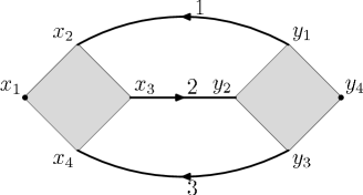
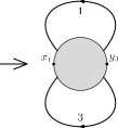
Figure 1: The first Filk Move: the line $2$ is reduced; the two initial vertices are glued up into a “fatter” final one

Repeating this operation for the $n-1$ tree lines, one obtains a single final vertex with all the loop lines hooked to it - a rosette. If a rosette has only one face we refer to it as to a super-rosette (see [14]).

Let us notice that the rosette can be considered as a vertex and one can write down its vertex factor, as done for any vertex entering some Feynman graph. We refer to it as to the rosette factor.

Furthermore, let us remark that the order relations defined above do not change when performing this first Filk move. Thus, as observed in section $3.1$ of [10] one has

Sign Alternation: Signs “+” and “-” alternate when turning around the rosette.

We also define $\ell<\ell^{\prime}$ if the starting point of $\ell$ precedes the end point of $\ell^{\prime}$ in the rosette.

Finally, once we choose a root and an orientation around the rosette, we can define the sign of a loop line $\varepsilon(\ell_{w})$ as $+1$ if the loop line goes in the same sense as the rosette orientation and $-1$ if it does not.

II.4 Parametric Representation for the Noncommutative Model

Note that, as pointed out in [14], the first polynomial in the noncommutative case is the determinant of the quadratic form integrated over all internal positions of the graph save one. One has thus to chose a particular “root” vertex whose position is not integrated. We denote this particular vertex by $\bar{V}$.

Let us now generalize the notions (II.9) of short and long variables at the level of the whole Feynman graph. For this purpose we define the $(L\times 4)$-dimensional incidence matrix $\varepsilon^{V}$ for each of the vertices $V$. Since the graph is orientable (in the sense defined in subsection II.3 above) we can choose

$$\varepsilon_{\ell i}^{V}=(-1)^{i+1},\mbox{ if the line $\ell$ hooks to the vertex $V$ at corner $i$.}$$ (II.16)

We also put

$$\eta^{V}_{\ell,i}=|\varepsilon^{V}_{\ell,i}|,\mbox{ }V=1,\ldots,n,\,\ell=1,\ldots,L\mbox{ and }i=1,\ldots,4.$$

One now has

$$v_{\ell} = \frac{1}{\sqrt{2}}\sum_{V}\sum_{i}\eta^{V}_{\ell i}x^{V}_{i},$$

$$u_{\ell} = \frac{1}{\sqrt{2}}\sum_{V}\sum_{i}\varepsilon^{V}_{\ell i}x^{V}_{i}.$$ (II.17)

Conversely, one has

$$x^{V}_{i}=\frac{1}{\sqrt{2}}\left(\eta^{V}_{\ell i}v_{\ell}+\varepsilon^{V}_{\ell i}u_{\ell}\right).$$

Let us now express the amplitude $\cal A$ of such a noncommutative graph with the help of these long and short variables. One has to put together the expressions of all the propagators (II.11) and vertices (II.12). Moreover, in order to avoid the $\sqrt{2}$ factors, we rescale the external positions $x_{e}$ to $\bar{x}_{e}$ and the hypermomenta $p_{V}$ to $\bar{p}_{V}$. One has:

$${\cal A}_{G}(x_{e}) = K\int\prod_{l}{d\alpha_{l}}\frac{(1-t_{\ell}^{2})^{2}}{t_{\ell}^{2}}\int\prod_{i\in{\cal I}}dx_{i}\prod_{V}dp_{V}\ e^{-\frac{\tilde{\Omega}}{2}\coth(\frac{\alpha_{\ell}}{2})u_{l}^{2}+i\tilde{\Omega}u_{\ell}\wedge v_{\ell}}$$

$$e^{{i}\sum_{1\leq i<j\leq 4}(-1)^{i+j+1}(\eta_{\ell i}^{V}v_{\ell}+\varepsilon^{V}_{\ell i}u_{\ell})\Theta^{-1}(\eta_{\ell^{\prime}j}^{V}v_{\ell^{\prime}}+\varepsilon_{\ell^{\prime}j}^{V}u_{\ell^{\prime}})}\ e^{\bar{p}_{\bar{V}}\sigma\sum(\eta_{\ell i}^{V}v_{\ell}+\varepsilon_{\ell i}u_{\ell})}$$

$$e^{2i[\sum_{i\neq e}\omega(i,e)(\eta^{V}_{\ell i}v_{\ell}+\epsilon_{\ell i}^{V}u_{\ell})\Theta^{-1}\bar{x}_{e}]+4i\sum_{e<e^{\prime}}\bar{x}_{e}\theta^{-1}\bar{x}_{e^{\prime}}+\sum_{e\in V}\bar{p}_{V}\sigma(-1)^{e+1}\bar{x}_{e}}\ ,$$

with $K$ some inessential normalization constant and $\omega(i,e)=1$ if $i<e$ and $-1$ if $i>e$. Singling out the root vertex $\bar{V}$, we write

$${\cal A}_{G}(x_{e},\bar{p}_{\bar{V}}) = K\int\prod_{l}{d\alpha_{l}}\frac{(1-t_{\ell}^{2})^{2}}{t_{\ell}^{2}}\int\prod_{i\in{\cal I}}dx_{i}\prod_{V\neq\bar{V}}dp_{V}\ e^{-\frac{\tilde{\Omega}}{2}\coth(\frac{\alpha_{\ell}}{2})u_{l}^{2}+i\tilde{\Omega}u_{\ell}\wedge v_{\ell}}$$

$$e^{{i}\sum_{1\leq i<j\leq 4}(-1)^{i+j+1}(\eta_{\ell i}^{V}v_{\ell}+\varepsilon^{V}_{\ell i}u_{\ell})\Theta^{-1}(\eta_{\ell^{\prime}j}^{V}v_{\ell^{\prime}}+\varepsilon_{\ell^{\prime}j}^{V}u_{\ell^{\prime}})}\ e^{\bar{p}_{\bar{V}}\sigma\sum(\eta_{\ell i}^{V}v_{\ell}+\varepsilon_{\ell i}u_{\ell})}$$

$$e^{2i[\sum_{i\neq e}\omega(i,e)(\eta^{V}_{\ell i}v_{\ell}+\epsilon_{\ell i}^{V}u_{\ell})\Theta^{-1}\bar{x}_{e}]+4i\sum_{e<e^{\prime}}\bar{x}_{e}\theta^{-1}\bar{x}_{e^{\prime}}+\sum_{e\in V}\bar{p}_{V}\sigma(-1)^{e+1}\bar{x}_{e}}\ .$$

From now on, in order to simplify notations, we forget the bar over the rescaled variables $\bar{x}_{e}$ and $\bar{p}$, but we keep the notation $\bar{V}$ for the chosen root.

One can write the amplitude (II.4) in the condensed way

$${\cal A}_{G}=\int\big{[}\frac{1-t^{2}}{t}\big{]}^{2}d\alpha\int dxdpe^{-\frac{\Omega}{2}XGX^{t}}$$ (II.20)

where

$$X=\begin{pmatrix}x_{e}&p_{\bar{V}}&u&v&p\\ \end{pmatrix}\ \ ,\ \ G=\begin{pmatrix}M&P\\ P^{t}&Q\\ \end{pmatrix}\ .$$ (II.21)

Furthermore, performing the Gaussian integration one obtains:

$${\cal A}_{G}=\int\big{[}\frac{1-t^{2}}{t}\big{]}^{2}d\alpha\frac{1}{\sqrt{{\rm det}Q}}e^{-\frac{\tilde{\Omega}}{2}\begin{pmatrix}x_{e}&\bar{p}\\ \end{pmatrix}[M-PQ^{-1}P^{t}]\begin{pmatrix}x_{e}\\ \bar{p}\\ \end{pmatrix}}\ .$$ (II.22)

This form allows to define the polynomials $HU$ and $HV$, the noncommutative analogs of $U$ and $V$ (see (II.2) and resp. (II.3)). One can write

$${\cal A}_{G}(x_{e})=K\int_{0}^{\infty}\prod_{l}[d\alpha_{l}(1-t_{l}^{2})^{2}]HU_{G}(t)^{-2}e^{-\frac{HV_{G}(t,x_{e})}{HU_{G}(t)}},$$ (II.23)

and resp.

$${\cal A}_{G}(x_{e},\;p_{\bar{V}})=K^{\prime}\int_{0}^{\infty}\prod_{l}[d\alpha_{l}(1-t_{l}^{2})^{2}]HU_{G,\bar{v}}(t)^{-2}e^{-\frac{HV_{G,\bar{V}}(t,x_{e},p_{\bar{V}})}{HU_{G,\bar{V}}(t)}},$$ (II.24)

Note that we refer to the polynomials $HU$ and $HV$ as to hyperbolic polynomials, since they are polynomials in the set of variables $t_{\ell}$ ($\ell=1,\ldots,L$), the hyperbolic tangent of the half-angle of the parameter $\alpha_{\ell}$ associated to each propagator line (see (II.10)).

Using now (II.22) and (II.24) the polynomial $HU_{G,\bar{V}}$ writes

$$HU_{G,\bar{V}}=({\rm det}\,Q)^{\frac{1}{4}}\prod_{\ell=1}^{L}t_{\ell}\ .$$ (II.25)

III The First Hyperbolic Polynomial

We now proceed with the analysis of the polynomial $HU_{G,\bar{V}}$ above, the study of the polynomial $HU_{G}$ being analogous. For this purpose we take a closer look at the matrix $Q$, matrix which can be read out of the developed expression (II.4). Note that the $(4(2L+n-1))$-dimensional matrix $Q$ can be written as

$$Q=A\otimes I_{4}-B\otimes\sigma$$ (III.1)

where $A$ is a $(2L+n-1)$-dimensional diagonal matrix and $B$ is an antisymmetric matrix of the same dimension. In [14] it has been proven that for a matrix of the form (III.1) one has

$$\det Q=[\det(A+B)]^{4}.$$ (III.2)

which, using (II.25) leads to

$$HU_{G,\bar{V}}={\rm det}(A+B)\prod_{\ell=1}^{L}t_{\ell}$$ (III.3)

Let us now study both the diagonal $A$ and the antisymmetric $B$ parts of $Q$.

One has

$$A=\begin{pmatrix}S&0&0\\ 0&0&0\\ 0&0&0\\ \end{pmatrix}$$ (III.4)

where $S$ is a $L-$dimensional diagonal matrix with elements $(1+t_{\ell}^{2})\setminus(2t_{\ell})$.

The antisymmetric part $B$ writes

$$B=\begin{pmatrix}{s}E&C\\ -C^{t}&0\\ \end{pmatrix}\$$ (III.5)

with

$$s=\frac{2}{\theta\tilde{\Omega}}=\frac{1}{\Omega}$$

and

$$C_{\ell V}=\begin{pmatrix}\sum_{i=1}^{4}(-1)^{i+1}\epsilon^{V}_{\ell i}\\ \sum_{i=1}^{4}(-1)^{i+1}\eta^{V}_{\ell i}\\ \end{pmatrix}\ ,$$ (III.6)

$$E=\begin{pmatrix}E^{uu}&E^{uv}\\ E^{vu}&E^{vv}\\ \end{pmatrix},$$ (III.7)

where

$$E^{vv}_{\ell,\ell^{\prime}} = \sum_{V}\sum_{i,j=1}^{4}(-1)^{i+j+1}\omega(i,j)\eta_{\ell i}^{V}\eta_{\ell^{\prime}j}^{V},$$

$$E^{uu}_{\ell,\ell^{\prime}} = \sum_{V}\sum_{i,j=1}^{4}(-1)^{i+j+1}\omega(i,j)\epsilon_{\ell i}^{V}\epsilon_{\ell^{\prime}j}^{V},$$

$$E^{uv}_{\ell,\ell^{\prime}} = \sum_{V}\sum_{i,j=1}^{4}(-1)^{i+j+1}\omega(i,j)\epsilon_{\ell i}^{V}\eta_{\ell^{\prime}j}^{V}+2\Omega\delta_{\ell\ell^{\prime}}.$$ (III.8)

Note that $\omega$ is the antisymmetric matrix for whom $\omega(i,j)=1$ if $i<j$.

Finally in order to have the integer expression (III.6) of the matrix $C$ coupling the $u$ and $v$ variables, we have rescaled by $s$ the hypermomenta $p_{V}$.

We also define the integer entries matrix:

$$B^{\prime}=\begin{pmatrix}E&C\\ -C^{t}&0\\ \end{pmatrix}\ .$$ (III.9)

We denote by $|I|$ the cardinal of the set $I$. Let us now state the following lemma:

Lemma III.1

With $A$ and $B$ given by (III.4) and (III.5)

$$\ \det(A+B)=\sum_{\begin{subarray}{c}I\subset\{1\dotsc L\},\\ n+|I|\;{\rm odd}\end{subarray}}(s^{-1})^{|I|+n-1-2L}n^{2}_{I}\prod_{l\in I}\frac{1+t_{\ell}^{2}}{2t_{\ell}}$$ (III.10)

with $n_{I}=\mathrm{Pf}(B^{\prime}_{\widehat{I}})$, the Pfaffian of the matrix $B^{\prime}$ above with deleted lines and columns $I$ among the first $L$ indices (corresponding to short variables $u$).

Proof: The proof is straightforward, being just a particular case of Lemma III.3 of [14]. $\Box$

Let us now define the integer

$$k_{I}=|I|-L-F+1.$$ (III.11)

Recalling that $2-2g=n-L+F$ one can use (II.25), (III.2) and Lemma III.1 above to obtain

$$HU_{G,{\bar{V}}}(t) = \sum_{\begin{subarray}{c}I\subset\{1\dotsc L\},\\ n+|I|\;{\rm odd}\end{subarray}}s^{2g-k_{I}}\ n_{I}^{2}\prod_{l\in I}\frac{1+t_{\ell}^{2}}{2t_{\ell}}\prod_{l^{\prime}\in\{1,\ldots,L\}}t_{l^{\prime}}\ .$$ (III.12)

Leading Terms in the First Polynomial

By leading terms we understand the terms of (III.12) which have the highest global degree in the $t_{1},\ldots,t_{L}$ variables. It is these terms that govern power counting.

To obtain these leading terms one needs to express the $I$ set in the development (III.12) of $HU_{G,{\bar{V}}}$. If one takes $I=\{1,\ldots,L\}$ then the corresponding Pfaffian is $0$ if $F\geq 2$ and $2^{g}$ iff $F=1$ (by Lemma III.4 of [14]).

Let us now consider $F\geq 2$. We take

$$I=\{1,\ldots,L\}-J_{0}$$ (III.13)

where $J_{0}$ is an admissible set in the sense defined in [14], i.e.

• it contains a tree $\tilde{T}$ in the dual graph and

• its complement contains a tree $T$ in the direct graph

Then the rosette obtained by removing the lines of $J$ and contracting the lines of $T$ is a super-rosette, that is a rosette with exactly one face (see subsection II.3).

In [14] it was proven that

$$F-1\leq|J_{0}|\leq F-1+2g.$$ (III.14)

Thus, the matrix $B^{\prime}$ corresponding to (III.13) has an even size, which we denote by $d$.

We take the admissible set $J_{0}$ such that $|J_{0}|=F-1$. One then has: $d=(n-1)+L+(F-1)$.

From now on, amongst the long variables $v$ we distinguish between the $n-1$ ones corresponding to the tree lines (which we continue to call $v$) and the $L-(n-1)$ ones corresponding to the loop lines (which we refer to as to $w$ variables).

The determinant of $B^{\prime}$ writes as a Grassmannian integral

$${\rm det}B^{\prime}=\int d\bar{\psi}^{u}_{1}d\psi^{u}_{1}\ldots d\bar{\psi}^{u}_{F-1}d\psi^{u}_{F-1}d\bar{\psi}^{w}_{1}d\psi^{w}_{1}\ldots d\bar{\psi}^{w}_{F-1}d\psi^{w}_{F-1}$$

$$d\bar{\psi}^{v}_{1}d\psi^{v}_{1}\ldots d\bar{\psi}^{v}_{n-1}d\psi^{v}_{n-1}d\bar{\psi}^{p}_{1}d\psi^{p}_{1}\ldots d\bar{\psi}^{p}_{n-1}d\psi^{p}_{n-1}e^{-\sum_{i,j=1}^{d}\bar{\zeta}_{i}b^{\prime}_{ij}\zeta_{j}}$$ (III.15)

where by $\zeta$ in the exponent we denote a generic Grassmannian in the set $\{\psi^{u},\psi^{w},\psi^{v},\psi^{p}\}$. Integrating over the Grassmannian variables $\bar{\psi}^{p}_{i},\psi^{p}_{i}$ ($i=1,\ldots,n-1$) one gets

$${\rm det}B^{\prime}=\int d\bar{\psi}^{u}_{1}d\psi^{u}_{1}\ldots d\bar{\psi}^{u}_{F-1}d\psi^{u}_{F-1}d\bar{\psi}^{w}_{1}d\psi^{w}_{1}\ldots d\bar{\psi}^{w}_{F-1}d\psi^{w}_{F-1}$$

$$d\bar{\psi}^{v}_{1}d\psi^{v}_{1}\ldots d\bar{\psi}^{v}_{n-1}d\psi^{v}_{n-1}X_{1}^{v}\bar{X}_{1}^{v}\ldots X_{n-1}^{v}\bar{X}_{n-1}^{v}e^{-\sum_{i,j=1}^{(F-1)+L}\bar{\psi}_{i}b^{\prime}_{ij}\psi_{j}}$$ (III.16)

with

$$X_{1}^{v} = C_{1,1}\psi^{u}_{1}+\ldots C_{L+(F-1),1}\psi^{v}_{n-1},$$

$$\bar{X}_{1}^{v} = C_{1,1}\bar{\psi}^{u}_{1}+\ldots C_{L+(F-1),1}\bar{\psi}^{v}_{n-1},$$

$$\ldots$$

$$X_{n-1}^{v} = C_{1,n-1}\psi^{u}_{1}+\ldots C_{L+(F-1),n-1}\psi^{v}_{n-1},$$

$$\bar{X}_{n-1}^{v} = C_{1,n-1}\bar{\psi}^{u}_{1}+\ldots C_{L+(F-1),n-1}\bar{\psi}^{v}_{n-1}.$$ (III.17)

Note that each pair $X_{i},\bar{X}_{i}$ ($i=1,\ldots,n-1$) corresponds to some vertex $i$ (which is of course different of the root vertex). Let us now put

$$\varepsilon_{j}\chi^{v}_{j} = X^{v}_{j}+\sum\varepsilon(k)X^{v}_{k},$$

$$\varepsilon_{j}\bar{\chi}^{v}_{j} = \bar{X}^{v}_{j}+\sum\varepsilon(k)\bar{X}^{v}_{k}$$ (III.18)

where the sign $\varepsilon_{j}$ is defined in Appendix A and the summation is performed on all the $X_{k}$ corresponding to the vertices entering or exiting the branch of the vertex corresponding to $X^{v}_{j}$.

One can now prove (see Appendix A) that the change of variable (III) is equivalent to

$$\psi^{v}_{k} = \chi^{v}_{k}-\varepsilon(k)\left[\sum\psi^{u}_{\ell}+\sum\varepsilon_{k}(\ell^{\prime})\psi^{w}_{\ell^{\prime}}\right],$$

$$\bar{\psi}^{v}_{k} = \bar{\chi}^{v}_{k}-\varepsilon_{k}\left[\sum\bar{\psi}^{u}_{\ell}+\sum\varepsilon_{k}(\ell^{\prime})\bar{\psi}^{w}_{\ell^{\prime}}\right],$$ (III.19)

where $\varepsilon(k)$ is the sign of the tree line associated to the vertex $k$ and $\varepsilon_{k}(\ell^{\prime})$ is the sign of the loop line $\ell^{\prime}$ which enters or exits the branch associated to the vertex $k$ (see subsection II.3).

Note that the form (III) of this change of variable leads directly to

$$X_{1}^{v}\bar{X}_{1}^{v}\ldots X^{v}_{n-1}\bar{X}^{v}_{n-1}=\chi_{1}^{v}\bar{\chi}_{1}^{v}\ldots\chi^{v}_{n-1}\bar{\chi}^{v}_{n-1}.$$ (III.20)

Furthermore (III) shows that the Jacobian of this triangular change of variables is $1$.

Let us remark here that the antisymmetric character of the matrix is preserved.

The determinant (III) rewrites as

$${\rm det}\,B^{\prime}=\int\bar{d}\bar{\psi}^{u}_{1}d\psi^{u}_{1}\ldots\bar{d}\bar{\psi}^{u}_{F-1}d\psi^{u}_{F-1}d\bar{\psi}^{w}_{1}d\psi^{w}_{1}\ldots d\bar{\psi}^{w}_{F-1}d\psi^{w}_{F-1}$$

$$d\bar{\chi}^{v}_{1}d\chi^{v}_{1}\ldots d\bar{\chi}^{v}_{n-1}d\chi^{v}_{n-1}\chi_{1}\bar{\chi}_{1}\ldots\chi_{n-1}\bar{\chi}_{n-1}e^{-\sum_{i,j=1}^{(F-1)+L}\bar{\zeta}_{i}b^{\prime}_{ij}\zeta_{j}}$$ (III.21)

where the general notation $\zeta$ denotes the Grassmannian variables belonging to the set $\{\psi^{u},\psi^{w},\chi^{v}\}$ and the matrix elements $b^{\prime}_{ij}$ are obtained from the previous ones by the change of variables (III).

The presence of the factor $\chi_{1}\bar{\chi}_{1}\ldots\chi_{n-1}\bar{\chi}_{n-1}$ in the Grassmann integral of (III) selects only the terms with no $\chi_{1}\bar{\chi}_{1}\ldots\chi_{n-1}\bar{\chi}_{n-1}$ in the development of the exponential.

Thus we end up with an antisymmetric matrix of type

$$B^{\prime}=\begin{pmatrix}E^{\prime uu}\ E^{\prime uw}\\ E^{\prime wu}\ E^{\prime ww}\end{pmatrix}\ .$$ (III.22)

As stated above, the elements of this matrix are obtained after performing the change of variable (III). This is nothing but the reduction of the graph via the first Filk move, reduction which has as result the rosette vertex of the graph. One can thus just read the elements of the matrix (III.22) from the rosette factor of the corresponding graph (see subsection II.3) .

Let us recall that

$$L=(n-1)+(F-1)+2g.$$ (III.23)

This leads to a distinction between the case $g=0$ and the case $g\geq 1$ (the non-planar case). We first treat the planar regular Feynman graphs.

III.1 The planar regular case

Since $g=0$, the matrix $B^{\prime}$ in (III.22) is a $2(F-1)-$dimensional matrix.

Let us now give the rosette factor of a planar regular graph, a result firstly obtained in [10], presented here under the form of Corollary $3.4$ of [11]:

$$\delta\big{(}\sum_{k=1}^{N}(-1)^{k+1}x_{k}+\sum_{l\in{\cal T}\cup{\cal L}}u_{l}\big{)}\,\exp\imath\varphi$$ (III.24)

where

$$\varphi=\ \varphi_{E}+\varphi_{X}+\varphi_{U},$$

$$\varphi_{E}=\ 2\sum_{i<j,\,i,j=1}^{N}(-1)^{i+j+1}x_{i}\Theta^{-1}x_{j},$$

$$\varphi_{X}=\ 2\sqrt{2}\sum_{k=1}^{N}\sum_{\begin{subarray}{c}\ell{\prec}k\end{subarray}}(-1)^{k+1}x_{k}\Theta^{-1}u_{l}+2\sqrt{2}\sum_{\ell{\succ}k}u_{l}\Theta^{-1}(-1)^{k+1}x_{k},$$

$$\varphi_{U}=\ 2\sum\limits_{\cal T}\epsilon(l)v_{l}\Theta^{-1}u_{l}+2\sum\limits_{\cal L}\epsilon(\ell)w_{\ell}\Theta^{-1}u_{\ell}$$

$$+4\sum\limits_{\ell\subset\ell^{\prime},\ell^{\prime}\in{\cal L}}\epsilon(\ell^{\prime})w_{\ell^{\prime}}\Theta^{-1}u_{l}+4\sum\limits_{\begin{subarray}{c}\ell\prec\ell^{\prime}\end{subarray}}u_{l^{\prime}}\Theta^{-1}u_{l}.$$

Note the difference in the numerical factors with respect to [11] or [10], difference appearing from the definition (II.9) of the short and long variables.

The rosette factor (III.24) leads to the following results:

Lemma III.2

The block $E^{\prime ww}$ in (III.22) is identically zero.

Proof: It is straightforwrd from (III.24). This expresses the fact that in a rosette of a planar graph the loop lines never cross each others. $\Box$

Lemma III.3

The lower triangular block of $E^{\prime uw}$ is identically zero.

Proof: One sees from (III.24) that $E^{\prime uw}_{\ell\ell^{\prime}}\neq 0$ if $\ell\subset\ell^{\prime}$. Ordering now the loop lines one obtains the result. $\Box$

Lemma III.4

$$E^{\prime uw}_{\ell\ell}=2\left(\Omega-\epsilon(\ell)\right)$$

Proof: Before the reduction of the matrix via the first Filk move, one has $E^{uw}_{\ell\ell}=2\Omega$ (coming from the propagator). The contribution obtained from the first Filk move reduction of the tree is read from (III.24), thus completing the proof. $\Box$

Let us also state:

Lemma III.5

Let $M$ be a $2d$-dimensional antisymmetric matrix such that

• $m_{i,j}=0,\,i=2,\ldots,d$, $d+1\leq j\leq d+i-1$;

• $m_{i,j}=0,\,i=d+2,\ldots,2d$, $d+1\leq j\leq i-1$.

Then

$${\rm det}M=(m_{1,d+1}m_{2,d+2},\ldots,m_{d,2d})^{2}.$$ (III.27)

Proof: We develop the determinant on its first line. The first contribution to be considered is the one of $m_{1,2}$. We now develop the remaining determinant on its first line and chose, lets say, the contribution of $m_{2,3}$. We continue this procedure until we arrive to the contribution of the factor $m_{d-1,d}$. From the first line of the remaining determinant, the only non-zero element is $m_{d,2d}$. However, its corresponding determinant is zero (the determinant of a zero-matrix).

Following the same type of arguments one can show that the only non-zero contribution in the determinant is the one in (III.27). $\Box$

We can now put all the pieces together. By Lemmas III.2, III.3 and III.4 one sees that the matrix $B^{\prime}$ given in (III.22) is exactly of the form of Lemma III.5. We have thus proved:

Proposition III.1

$${\rm Pf}\,B^{\prime}=\prod\limits_{\ell\in\cal L}2\left(\Omega-\epsilon(\ell)\right).$$ (III.28)

Let us now deal with the case of non-planar Feynman graphs, keeping in mind that the interest for the planar non-regular case will be underlined in the next section.

III.2 The non-planar case

Now since $g\geq 1$ the matrix $B^{\prime}$ of (III.22) is a $\left(2(F-1)+2g\right)$-dimensional matrix (see (III.23)). We divide the $(F-1)+2g$ loop variables $w$ in two categories:

• $(F-1)$ “face” variables, which we denote by $w^{f}$ and

• $g$ pairs of “genus” variables, which we denote by $w^{g}$.

Let us recall here the notion of “nice-crossing” [14] for a pair of lines of a rosette obtained from a Feynman graph which is not regular planar. Such a pair of lines $\ell_{1}$ and $\ell_{2}$ realize a nice-crossing if the start of $\ell_{2}$ immediately precedes the end of $\ell_{1}$ in the rosette.

Choosing a tree in the dual graph, the respective $F-1$ lines are our so-called face-lines (see above). The remaining rosette has only one face (i.e. it is a super-rosette, see subsection II.3) and hence one can state that the $g$ pairs of lines form the $g$ nice-crossings of the rosette.

After the reduction of the graph via the first Filk move (resp. the change of variable (III)) the entries of the matrix $B^{\prime}$ (given again by the rosette factor, as above) are more complicated that in the planar regular case.

The general form of the matrix $B^{\prime}$ is

$$B^{\prime}=\begin{pmatrix}E^{\prime uu}&E^{\prime uw^{f}}&E^{\prime uw^{g}}\\ E^{\prime w^{f}u}&E^{\prime w^{f}w^{f}}&E^{\prime w^{f}w^{g}}\\ E^{\prime w^{g}u}&E^{\prime w^{g}w^{f}}&E^{\prime w^{g}w^{g}}\end{pmatrix}.$$ (III.29)

As before, we can read the entries of this matrix from the rosette factor, which now writes (see Corollary $3.3$ of [11])

$$\delta\big{(}\sum_{k=1}^{N}(-1)^{j_{k}+1}s_{j_{k}}+\sum_{l\in{\cal T}\cup\cal L}u_{l}\big{)}\,\exp\imath\varphi,$$ (III.30)

with

$$\varphi=\ \varphi_{E}+\varphi_{X}+\varphi_{U}+\varphi_{W},$$

$$\varphi_{E}=\ 2\sum_{k<l=1}^{N}(-1)^{j_{k}+j_{l}+1}s_{j_{k}}\Theta^{-1}s_{j_{l}},$$

$$\varphi_{X}=\ 2\sqrt{2}\sum_{k=1}^{N}\sum_{\begin{subarray}{c}\ell\prec j_{k}\end{subarray}}(-1)^{j_{k}+1}s_{j_{k}}\Theta^{-1}u_{l}+2\sqrt{2}\sum_{\ell\succ j_{k}}(-1)^{j_{k}+1}u_{l}\Theta^{-1}s_{j_{k}},$$

$$\varphi_{U}=\ 2\sum_{{\cal T}}\epsilon(l)v_{l}\Theta^{-1}u_{l}+2\sum_{{\cal L}}\epsilon(\ell)w_{\ell}\Theta^{-1}u_{\ell}$$

$$+2\sum_{\ell\ltimes\ell^{\prime},\,\ell,\ell^{\prime}\in{\cal L}}\left[\epsilon(\ell)w_{\ell}\Theta^{-1}u_{\ell^{\prime}}+\epsilon(\ell^{\prime})w_{\ell^{\prime}}\Theta^{-1}u_{\ell}\right]+4\sum_{\begin{subarray}{c}\ell\subset\ell^{\prime}\end{subarray},\,\ell^{\prime}\in{\cal L}}\epsilon(\ell^{\prime})w_{\ell^{\prime}}\Theta^{-1}u_{l}$$

$$+4\sum_{\begin{subarray}{c}\ell\prec\ell^{\prime}\end{subarray}}u_{l^{\prime}}\Theta^{-1}u_{l}+2\sum_{\begin{subarray}{c}\ell\ltimes\ell^{\prime}\,\ell,\ell^{\prime}\in{\cal L}\end{subarray}}u_{\ell^{\prime}}\Theta^{-1}u_{\ell},$$

$$\varphi_{W}=\ \sqrt{2}\sum_{\begin{subarray}{c}\ell\supset j_{k},\,\ell\in{\cal L}\end{subarray}}(-1)^{j_{k}}s_{j_{k}}\Theta^{-1}\epsilon(\ell)w_{\ell}+2\sum_{\begin{subarray}{c}\ell\ltimes\ell^{\prime},\,\ell,\ell^{\prime}\in{\cal L}\end{subarray}}\epsilon(\ell^{\prime})w_{\ell^{\prime}}\Theta^{-1}\epsilon(\ell)w_{\ell}.$$

By a direct inspection of (III.30), one notices that the coupling between:

• the $u_{\ell}$’s and the $w^{f}_{\ell^{\prime}}$’s for whom $\ell\subset\ell^{\prime}$ and

• the $w^{f}$’s themselves

is trivial. Furthermore, the coupling between any $u_{\ell}$ and its corresponding $w^{f}_{\ell}$ is $2(\Omega-\epsilon(\ell))$. Moreover (as also observed in [14]), the coupling between the $w^{g}$ variables has a Jordan-block form.

Nevertheless, the situation is more complicated than in the planar regular case because the new elements $w^{g}$ couple in a non-trivial way with the rest of the matrix. In order to bring these new couplings to a trivial form, we perform a sort of “fourth Filk move”, which generalizes the third Filk move introduced in [14].

Let us first treat the case of just one pair of genus lines, say $\ell^{g}_{1}\ltimes\ell^{g}_{2}$. First notice that if some face line crosses such a pair of genus lines, then it must cross both of the lines of the pair. Indeed, assuming it crosses only one of the genus lines, one can see on the rosette that an additional face is added, which cannot be the case.

The fourth Filk move we propose here is the following change of Grassmannian variables:

$$\eta^{w^{g}}_{1}=\psi^{w^{g}}_{1}+\sum_{\ell^{\prime}<\ell_{2}^{g};\,\ell^{\prime}\cap\ell_{2}^{g}}\psi^{w^{f}}_{\ell^{\prime}}-\sum_{\ell^{\prime\prime}>\ell_{2}^{g};\ell^{\prime\prime}\cap\ell_{2}^{g}}\psi^{w^{f}}_{\ell^{\prime\prime}}$$

$$\ \ \ \ \ \ \ \ \ \ \ \ \ \ \ \ \ \ \ \ \ \ \ \ \ \ \ \ \ \ +\sum_{\ell^{\prime}<\ell_{2}^{g};\ell^{\prime}\cap\ell_{2}^{g}}\psi^{u}_{\ell^{\prime}}-\sum_{\ell^{\prime\prime}>\ell_{2}^{g};\ell^{\prime\prime}\cap\ell_{2}^{g}}\psi^{u}_{\ell^{\prime\prime}},$$

$$\eta^{w^{g}}_{2}=\psi^{w^{g}}_{2}-\sum_{\ell^{\prime}<\ell_{1}^{g};\,\ell^{\prime}\cap\ell_{1}^{g}}\psi^{w^{f}}_{\ell^{\prime}}+\sum_{\ell^{\prime\prime}>\ell_{1}^{g};\ell^{\prime\prime}\cap\ell_{1}^{g}}\psi^{w^{f}}_{\ell^{\prime\prime}}$$

$$\ \ \ \ \ \ \ \ \ \ \ \ \ \ \ \ \ \ \ \ \ \ \ \ \ \ \ \ \ \ -\epsilon(\ell^{g}_{1})\epsilon(\ell^{g}_{2})\left(-\sum_{\ell^{\prime}<\ell_{1}^{g};\ell^{\prime}\cap\ell_{1}^{g}}\psi^{u}_{\ell^{\prime}}+\sum_{\ell^{\prime\prime}>\ell_{1}^{g};\ell^{\prime\prime}\cap\ell_{1}^{g}}\psi^{u}_{\ell^{\prime\prime}}\right),$$

$$\bar{\eta}^{w^{g}}_{1}=\bar{\psi}^{w^{g}}_{1}+\sum_{\ell^{\prime}<\ell_{2}^{g};\,\ell^{\prime}\cap\ell_{2}^{g}}\bar{\psi}^{w^{f}}_{\ell^{\prime}}-\sum_{\ell^{\prime\prime}>\ell_{2}^{g};\ell^{\prime\prime}\cap\ell_{2}^{g}}\bar{\psi}^{w^{f}}_{\ell^{\prime\prime}}$$

$$\ \ \ \ \ \ \ \ \ \ \ \ \ \ \ \ \ \ \ \ \ \ \ \ \ \ \ \ \ \ +\sum_{\ell^{\prime}<\ell_{2}^{g};\ell^{\prime}\cap\ell_{2}^{g}}\bar{\psi}^{u}_{\ell^{\prime}}-\sum_{\ell^{\prime\prime}>\ell_{2}^{g};\ell^{\prime\prime}\cap\ell_{2}^{g}}\bar{\psi}^{u}_{\ell^{\prime\prime}},$$

$$\bar{\eta}^{w^{g}}_{2}=\bar{\psi}^{w^{g}}_{2}-\sum_{\ell^{\prime}<\ell_{1}^{g};\,\ell^{\prime}\cap\ell_{1}^{g}}\bar{\psi}^{w^{f}}_{\ell^{\prime}}+\sum_{\ell^{\prime\prime}>\ell_{1}^{g};\ell^{\prime\prime}\cap\ell_{1}^{g}}\bar{\psi}^{w^{f}}_{\ell^{\prime\prime}}$$ (III.31)

$$\ \ \ \ \ \ \ \ \ \ \ \ \ \ \ \ \ \ \ \ \ \ \ \ \ \ \ \ \ \ -\epsilon(\ell^{g}_{1})\epsilon(\ell^{g}_{2})\left(-\sum_{\ell^{\prime}<\ell_{1}^{g};\ell^{\prime}\cap\ell_{1}^{g}}\bar{\psi}^{u}_{\ell^{\prime}}+\sum_{\ell^{\prime\prime}>\ell_{1}^{g};\ell^{\prime\prime}\cap\ell_{1}^{g}}\bar{\psi}^{u}_{\ell^{\prime\prime}}\right).$$

As proven in [14], the terms in $\psi^{w}$ above will produce a trivial coupling between all the $w$ variables (except for the coupling between the two $w$ variables of the lines of a nice crossing coupling, which are not affected by (III.2); these coupling will keep their Jordan-block form mentioned above). Furthermore, notice that the new $\psi^{u}$ terms present in the fourth-Filk move (III.2) do not affect the couplings between the $\psi^{w}$’s (they just affect the lines and columns corresponding to the $u$ variables).

Let us now investigate the change produced by (III.2) in the rest of the couplings of the matrix. We start this investigation with the coupling between an $u_{\ell}$ variable and its corresponding $w^{f}_{\ell}$ variable. As mentioned above, before performing (III.2) this element has the value $2(\Omega-\epsilon(\ell))$. If the line $\ell$ does not cross the pair $\ell^{g}_{1},\ell^{g}_{2}$ then the change of variable (III.2) will not affect the element $E^{\prime uw^{f}}_{\ell}$. Suppose now that $\ell^{g}_{1}<\ell<\ell^{g}_{2}$ (the other cases being analogous). The effect of the $\psi^{w}$ terms in (III.2) on $E^{\prime uw^{f}}_{\ell,\ell}$ is the following:

$$E^{\prime uw^{f}}_{\ell,\ell}\to E^{\prime uw^{f}}_{\ell,\ell}+E^{\prime uw^{g}}_{u,1}+E^{\prime uw^{g}}_{u,2}.$$

The values of $E^{\prime uw^{g}}_{u,1}$ and $E^{\prime uw^{g}}_{u,2}$ can be read of (III.30) to be $2\epsilon(\ell^{g}_{1})$ and resp. $2\epsilon(\ell^{g}_{2})$. One can now distinguish several cases:

• $\epsilon(\ell^{g}_{1})\epsilon(\ell^{g}_{2})=-1$, the contributions of the two lines cancel each other and thus the entry $(u_{\ell},w^{f}_{\ell})$ does not change;

• $\epsilon(\ell^{g}_{1})\epsilon(\ell^{g}_{2})=1$, one can see from the sign alternation property (see subsection II.3) that if $\epsilon(\ell^{g}_{1})=1=\epsilon(\ell^{g}_{2})$ then $\epsilon(\ell)=-1$ (and thus the resp. entry changes from $2(\Omega+1)$ to $2(\Omega-1)$) or vice versa.

Now that this part of the change of variables (III.2) (concerning the $\psi^{w^{f}}$ variables) is completed, the part concerning the $\psi^{u}$’s in (III.2) do not change anymore the value of the $(u_{\ell},w^{f}_{\ell})$ entry. Indeed the new contribution is now given by the entries $(w^{f}_{\ell},w^{g}_{1})$ and $(w^{f}_{\ell},w^{g}_{2})$, which, as already stated above, are equal to $0$ after the third Filk move.

Using the same type of arguments one is able to prove that the coupling between the $u_{\ell}$’s and the $w^{f}_{\ell^{\prime}}$’s for which $\ell\subset\ell^{\prime}$ remains $0$ and furthermore that the $u$’s now couple trivially with the $w^{g}$’s.

Thus, the matrix (III.29) has now the form

$$\begin{pmatrix}E^{\prime\prime uu}&E^{\prime\prime uw^{f}}&0\\ E^{\prime\prime w^{f}u}&0&0\\ 0&0&E^{\prime\prime w^{g},w^{g}}\\ \end{pmatrix}$$ (III.32)

where $E^{\prime\prime w^{g},w^{g}}$ has a Jordan-block form and $E^{\prime\prime uw^{f}}$ has a lower-diagonal zero block and the elements on its diagonal are of the form $2(\Omega\pm 1)$. Hence the Pfaffian is $2^{g}\prod 2(\Omega\pm 1)$.

The case of several pairs of genus-lines which present nice-crossings is treated analogously. One performs a change of variables (III.2) for each of the $g$ pairs of lines. The trickier cases when a face-line crosses two pairs of genus-lines is shown by the sign alternation property (see subsection II.3) not to lead to a different result than above.

Using now (III.12) we can conclude this section with:

Theorem III.1

$$HU_{G,{\bar{V}}}(t)\geq\sum_{J_{0}\,{\rm admissible}}s^{2[g+(F-1)]}\ \left(2^{g}\prod 2(\Omega\pm 1)\right)^{2}$$

$$\prod_{l\in I}\frac{1+t_{\ell}^{2}}{2t_{\ell}}\prod_{l^{\prime}\in\{1,\ldots,L\}}t_{l^{\prime}}\ .$$ (III.33)

Let us firstly remark that the RHS above never vanishes for $\Omega\in[0,1[$.

As anounced in section I, this is the main result of our paper. Let us now argue on its meaning. Indeed, using now (II.24), one has an upper limit for the Feynman amplitude of any noncommutative graph $G$. Moreover, from this formula power counting follows easily, as exhibited in [14]. Through the method proposed in this section we obtain an exact power counting as function of the graph genus, hence an improvement with respect to [11].

Furthermore we observe that the dimension $D$ of space time would appear simply as a parameter in this representation. Therefore this work as well as [14] is the starting point to compute dimensional regularization and dimensional renormalization for all classes of scalar, LSZ or Gross-Neveu models.

Moreover, via our approach, richer topological information is obtained, since we deal with a positivity theorem on some “hypertrees” related to the admissible sets $J_{0}$. The expressions deduced in this section allow the generalization of the notion of “democracy” between (hyper)trees, also present in the case of commutative QFT (see (II.2)).

Let us end this section by another remark. A weaker result than Theorem III.1 can be obtained. This result does not require all the techniques used above and it just states that one has the same type of positivity and improved power counting but just for a smaller class of values for $\Omega\in[0,1[$, namely for the transcendent values of $\Omega$.

Indeed, the Pfaffians $n_{I}$ corresponding to the leading terms in (III.12) are integer coefficient polynomials in $\Omega$, of degree $F-1$:

$$n_{I}=\sum_{k=0}^{F-1}a_{k}\Omega^{k}.$$ (III.34)

Developing the Pfaffian $n_{I}$ one can identify the coefficient $a_{F-1}$ above as the Pfaffian $n_{I,J_{0}}$ of section III of [14] (corresponding to the admissible set $J_{0}$). Moreover, in Lemma III.5 of [14] it was proven that this coefficient is nonvanishing. Therefore, the polynomial (III.34) with integer coefficients can have only a finite number of algebraic roots. These roots could a priori vary when the graph varies, but none can be transcendent.

We can thus conclude that, for $\Omega$ a transcendent number, $n_{I}$ given by (III.34) never vanishes. Recall however that this is a weaker result than Theorem III.1, which holds for any $\Omega\in[0,1[$, transcendent or not.

IV The Second Hyperbolic Polynomial

We now proceed with the analysis of the second hyperbolic polynomial. As before, we focus on the study of $HV_{G,\bar{V}}$, the polynomial $HV_{G}$ being similar. This analysis follows the same lines of the one of section IV of [14].

Comparing (II.22) and (II.23) one has

$$\frac{HV_{G,\bar{V}}}{HU_{G,\bar{V}}}=\frac{\tilde{\Omega}}{2}\begin{pmatrix}x_{e}&p_{\bar{V}}\end{pmatrix}PQ^{-1}P^{t}\begin{pmatrix}x_{e}\\ p_{\bar{V}}\end{pmatrix}$$ (IV.1)

Note that we left aside the matrix $M$ appearing in (II.22) since it factorizes out of the integral.

As in the previous section, the entries of the matrix $P$ are read out of (II.4). Moreover $P$ has the same form as in [14].

The expression (III.1) of the matrix $Q$ implies that its inverse is:

$$Q^{-1}_{\tau\tau^{\prime}}=\frac{(A+B)^{-1}_{\tau\tau^{\prime}}+(A-B)^{-1}_{\tau\tau^{\prime}}}{2}\otimes I_{4}+\frac{(A-B)^{-1}_{\tau\tau^{\prime}}-(A+B)^{-1}_{\tau\tau^{\prime}}}{2}\otimes\sigma.$$ (IV.2)

One thus notices that we deal with a real part given by the $I_{4}$ terms and an imaginary part given by $\sigma$. As already mentioned in [14] we are interested here by the former, which leads to a hyperbolic polynomial that we denote by $HV^{R}_{G,\bar{V}}$.

Furthermore, let $\mathrm{Pf}(B_{\hat{K}\hat{\tau}})$ be the Pfaffian of the matrix obtained from $B$ by deleting the lines and columns in the set ${I,\tau}$ where $\tau\notin I$. Moreover we define $\epsilon_{I,\tau}$ to be the signature of the permutation obtained from $(1,\ldots,d)$ by extracting the positions belonging to $I$ and replacing them at the end in the order

$$1,\dotsc,d\rightarrow 1,\dotsc,\hat{i_{1}},\dotsc,\hat{i_{p}},\dotsc,\hat{i_{\tau}},\dotsc,d,i_{\tau},i_{p}\dotsc,i_{1}\,.$$ (IV.3)

Note that by $d$ we mean the dimension of the matrix (here $2L+n-1$) and by $p$ we mean the cardinal of $I$.

One has

Lemma IV.1

$$\frac{HV^{R}_{G,{\bar{V}}}}{HU_{G,{\bar{V}}}}(x_{e},p_{\bar{V}})=\frac{1}{HU_{G,{\bar{V}}}}\sum_{I}\prod_{\ell}t_{\ell}\prod_{i\in I}\frac{1+t_{i}^{2}}{2t_{i}}\Big{[}\sum_{e}x_{e}\sum_{\tau\notin K}P_{e\tau}\epsilon_{I\tau}\mathrm{Pf}(B_{\hat{I}\hat{\tau}})\Big{]}^{2}.$$

Proof: The proof is straightforward, being just a particular case of Lemma IV.1 of [14]. $\Box$

As in the previous section, we now proceed with the analysis of the leading terms in this sum.

Leading terms

As we have seen, the leading terms are given by the sets $I=\{1,\ldots,L\}\setminus J_{0}$, where $J_{0}$ is an admissible set.

The job to be done is the investigation of the conditions under which Pfaffians of type

$$\epsilon_{I\tau}\mathrm{Pf}(B_{\hat{K}\hat{\tau}})=\int\prod_{\alpha=1\dotsc d}d\chi_{\alpha}\prod_{i\in I}\chi_{i}\chi_{\tau}e^{-\frac{1}{2}\chi B\chi}\,,$$ (IV.4)

are nonzero.

As pointed out in [14], we first distinguish two types of graphs as

• the graphs which do not have any vertex with two opposite external legs and

• the graphs which have at least a vertex with two opposite external legs.

Regarding the former case, we follow exactly the reasoning of [14], and for some external position $x_{e}$ we introduce a dummy Grassmann variable in the Pfaffian integral, which once exponentiated can be interpreted as if we add a new line between $x_{e}$ and the root. We denote this modified graph by $G^{\prime}$. One thus has a one-to-one correspondence between the leading terms in $HV_{G,\bar{V}}$ and the leading terms of $HU_{G^{\prime},\bar{V}}$ in which the dummy line is chosen to be a tree line (see again subsection IV.1 of [14] for further details). Note that these leading terms were computed in section III here.

To any tree in $G^{\prime}$ which contains the above dummy line there corresponds a two-tree $T_{2}$ in $G$ (i.e. a tree without a line, the dummy one).

Let us now recall the definition of a 2-admissible set $J$ in $G$ as a set which satisfies the conditions:

• $J$ is admissible in $G$ and

• the dummy line is a tree of $G^{\prime}$ contained in the complement of $J$.

Now, as argued in [14], the graph obtained from $G$ by deleting the lines $\{1,\ldots,L\}\setminus J$ and contracting the two-tree $T_{2}$ has two faces, the one broken by the root and another one, which we denote by $F_{J}$. The bound analogous to (III.1) is

$$HV^{R}_{G,{\bar{v}}}(x_{e})\geq\sum_{J\ {\rm 2-admissible\ in}\ G}(s^{2[g^{\prime}+(F^{\prime}-1)]}\left(2^{g^{\prime}}\prod 2(\Omega\pm 1)\right)^{2}$$

$$\prod_{\ell\in I}\frac{1+t_{\ell}^{2}}{2t_{\ell}}\prod_{\ell^{\prime}}t_{\ell^{\prime}}[\sum_{e\in F_{J}}(-1)^{e}x_{e}]^{2}\;.$$ (IV.5)

The more complicated case of a graph containing at least a vertex with opposite external legs is more tricky because, as indicated in [14] one has a sum of two Pfaffians which could a priori cancel each other. These two Pfaffians correspond to two graphs $G_{1}^{\prime}$ of genus $g_{1}$ (obtained by adding a dummy line to $G$, as described above) and $G_{2}^{\prime}$ (with one line erased with respect to $G_{1}^{\prime}$) of genus $g_{2}=g_{1}-1$. However, the second one has an additional factor $s$ in its weight in the sum of Lemma IV.1 (see again section IV of [14] for details). In our case, checking the values of the $s$ and the $2$ factors (given by Theorem III.1 or (IV)) appearing in this sum one can easily see that no value of $\Omega$ can cancel it.

V Examples

For the seek of completeness, we give here some examples of planar regular, non-regular and finally non-planar graphs.

V.1 Planar regular graphs

We start be the simplest example, namely the $1-$loop graph. One has here $1$ vertex ($n=1$), one internal line ($L=1$) and two faces ($F=2$). Applying the methods described in this article, one finds, for the loop of Fig. 2

$$HU_{G,\bar{V}}=4s^{2}t(\Omega+1)^{2}.$$ (V.1)

and resp.

$$HU_{G,\bar{V}}=4s^{2}t(\Omega-1)^{2}.$$ (V.2)

for the loop of Fig. 3.

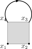
Figure 2: One loop, a first choice

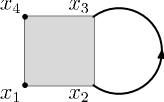
Figure 3: One loop, the second choice

Let us now go along to a more complicated case, the bubble graph (see Fig. 4) which has $n=2$, $L=2$ and $F=2$. One obtains:

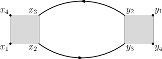
Figure 4: The bubble graph

$$HU_{G,\bar{V}}=2s^{2}(t_{1}+t_{2}+t_{1}^{2}t_{2}+t_{1}t_{2}^{2})(\Omega-1)^{2}.$$ (V.3)

For the sunshine graph (see Fig. 5) one has $n=2$, $L=3$, $F=3$ and

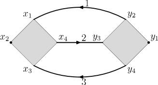
Figure 5: The sunshine graph

$$HU_{G,\bar{V}}=8(1+\Omega)^{2}\ s^{4}\left((-1+\Omega)^{2}t_{2}t_{3}+(-1+\Omega)^{2}t_{1}^{2}t_{2}t_{3}+\right.$$

$$\left.(1+\Omega)^{2}t_{1}(t_{2}+t_{3})(1+t_{2}t_{3})\right).$$ (V.4)

For the half-eye graph (see Fig. 6) one has $n=3$, $L=4$, $F=3$ and

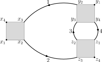
Figure 6: The half-eye Graph

$$HU_{G,\bar{V}}=4s^{4}(\Omega-1)^{2}(\Omega+1)^{2}[t_{3}t_{4}+t_{2}^{2}t_{3}t_{4}+t_{2}(t_{3}+t_{4}+t_{3}^{2}t_{4}+t_{3}t_{4}^{2})$$

$$+t_{1}^{2}\left(t_{3}t_{4}+t_{2}^{2}t_{3}t_{4}+t_{2}(t_{3}+t_{4}+t_{3}^{2}t_{4}+t_{3}t_{4}^{2})\right)$$

$$+t_{1}\left((1+t_{2}^{2})(t_{4}+t_{3}^{2}t_{4})+t_{3}\left(1+64s^{2}t_{2}t_{4}+t_{4}^{2}+t_{2}^{2}(1+t_{4}^{2})\right)\right)].$$ (V.5)

The most complicated example of a planar regular graph we consider is the eye-graph (see Fig. 7), with $n=4$, $L=6$, $F=4$.

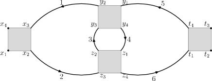
Figure 7: The eye graph

We obtain:

$$HU_{G,\bar{V}}=8\,{(-1+\Omega)}^{4}\,{(1+\Omega)}^{2}\,s^{6}\,({t_{3}}\,{t_{4}}\,({t_{5}}+{t_{6}})\,(1+{t_{5}}\,{t_{6}})$$

$$+{{t_{2}}}^{2}\,{t_{3}}\,{t_{4}}\,({t_{5}}+{t_{6}})\,(1+{t_{5}}\,{t_{6}})$$

$$+{t_{2}}\,({t_{4}}\,({t_{5}}+{t_{6}})\,(1+{t_{5}}\,{t_{6}})+{{t_{3}}}^{2}\,{t_{4}}\,({t_{5}}+{t_{6}})\,(1+{t_{5}}\,{t_{6}})$$

$$+{t_{3}}\,({t_{5}}+{t_{6}}+{t_{5}}\,{t_{6}}\,({t_{5}}+{t_{6}})+{{t_{4}}}^{2}\,({t_{5}}+{t_{6}})\,(1+{t_{5}}\,{t_{6}})$$

$$+{t_{4}}\,(1+64\,\Omega^{2}\,s^{2}\,{t_{5}}\,{t_{6}}+{{t_{6}}}^{2}+{{t_{5}}}^{2}\,(1+{{t_{6}}}^{2}))))$$

$$+{t_{1}}\,((1+{{t_{2}}}^{2})\,{t_{4}}\,({t_{5}}+{t_{6}})\,(1+{t_{5}}\,{t_{6}})$$

$$+(1+{{t_{2}}}^{2})\,{{t_{3}}}^{2}\,{t_{4}}\,({t_{5}}+{t_{6}})\,(1+{t_{5}}\,{t_{6}})+{t_{3}}\,((1+{{t_{2}}}^{2})\,({t_{5}}+{t_{6}})\,(1+{t_{5}}\,{t_{6}})$$

$$+(1+{{t_{2}}}^{2})\,{{t_{4}}}^{2}\,({t_{5}}+{t_{6}})\,(1+{t_{5}}\,{t_{6}})+{t_{4}}\,(1+{{t_{5}}}^{2}$$

$$+64\,\Omega^{2}\,s^{2}\,{t_{5}}\,{t_{6}}+(1+{{t_{5}}}^{2})\,{{t_{6}}}^{2}+64\,\Omega^{2}\,s^{2}\,{t_{2}}\,({t_{5}}+{t_{6}})\,(1+{t_{5}}\,{t_{6}})$$

$$+{{t_{2}}}^{2}\,(1+{{t_{5}}}^{2}+64\,\Omega^{2}\,s^{2}\,{t_{5}}\,{t_{6}}+(1+{{t_{5}}}^{2})\,{{t_{6}}}^{2}))))$$

$$+{{t_{1}}}^{2}\,({t_{3}}\,{t_{4}}\,({t_{5}}+{t_{6}})\,(1+{t_{5}}\,{t_{6}})+{{t_{2}}}^{2}\,{t_{3}}\,{t_{4}}\,({t_{5}}+{t_{6}})\,(1+{t_{5}}\,{t_{6}})$$

$$+{t_{2}}\,({t_{4}}\,({t_{5}}+{t_{6}})\,(1+{t_{5}}\,{t_{6}})+{{t_{3}}}^{2}\,{t_{4}}\,({t_{5}}+{t_{6}})\,(1+{t_{5}}\,{t_{6}})$$

$$+{t_{3}}\,({t_{5}}+{t_{6}}+{t_{5}}\,{t_{6}}\,({t_{5}}+{t_{6}})+{{t_{4}}}^{2}\,({t_{5}}+{t_{6}})\,(1+{t_{5}}\,{t_{6}})$$

$$+{t_{4}}\,(1+64\,\Omega^{2}\,s^{2}\,{t_{5}}\,{t_{6}}+{{t_{6}}}^{2}+{{t_{5}}}^{2}\,(1+{{t_{6}}}^{2})))))).$$ (V.6)

If one chooses the admissible set to be formed of the lines $3,4$ and $6$ the leading term has

$$n_{I}=8(\Omega+1)(\Omega-1)^{2}.$$ (V.7)

V.2 An example of a planar non-regular graph

Let us now show an example of a planar but not regular graph, the broken bubble graph (see Fig. 8). This graph has $n=2$, $L=2$, $F=2$ (and thus $g=0$) but both of the faces are broken by external lines (hence $B=2$).

One gets:

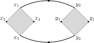
Figure 8: The broken bubble graph

$$HU_{G,\bar{V}}=2s^{2}[(t_{2}+t_{1}^{2}t_{2})(\Omega-1)^{2}+(t_{1}+t_{1}t_{2}^{2})(\Omega+1)^{2}].$$ (V.8)

V.3 Non-planar graphs

In order to investigate all possible cases, we conclude with some non-planar graphs. The simplest one we consider here is the non-planar sunshine graph (see Fig. 9) which has $n=2$, $L=3$ but $F=1$, and hence $g=1$. One gets:

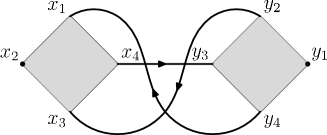
Figure 9: The non-planar sunshine graph

$$HU_{G,\bar{V}}=\frac{1}{2}s^{2}(1+16(1+\Omega^{2})^{2}s^{2}t_{2}t_{3}+t_{3}^{2}+t_{2}^{2}(1+t_{3}^{2})$$

$$+16(-1+2\Omega+\Omega^{2})^{2}s^{2}t_{1}(t_{2}+t_{3}+t_{2}^{2}t_{3}+t_{2}t_{3}^{2})$$

$$+t_{1}^{2}(1+16(1+\Omega^{2})^{2}s^{2}t_{2}t_{3}+t_{3}^{2}+t_{2}^{2}(1+t_{3}^{2})).$$

Let us consider the twisted-eye graph (see Fig. 10), which has $n=5$, $L=6$, $F=2$ and hence $g=1$.

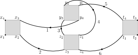
Figure 10: The twisted eye graph

If one chooses as the admissible set the set formed of the line $4$ or $6$ then one gets

$$n_{I}=2^{2}(\Omega-1).$$ (V.10)

The most complicated example we have considered is the Feynman graph of Fig. 11.

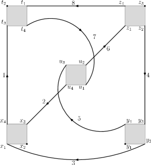
Figure 11: A more complicated non-planar graph

If one chooses the admissible set to be the set formed of the lines $7$ and $8$, one is able to calculate

$$n_{I}=8(\Omega-1)(\Omega+1).$$ (V.11)

Appendix A Proof of formula (III)

We now prove that the change of variables (III) is equivalent to the form (III). We first prove that the formula is true for a leaf vertex and then we proceed by induction to show that it is true for any vertex in the graph.

For some vertex $V$ one has (see (III)):

$$X_{V}^{v} = C_{1,V}\psi^{u}_{1}+\ldots C_{L+(F-1),V}\psi^{v}_{n-1},$$

When dealing with a leaf, one has only one non-zero entry $C_{i,V}$ corresponding to the set of variables $\psi^{v}$. Note that this variable corresponds to the line $\ell_{V}$ (see subsection II.3). We denote its corresponding $\psi^{v}$ variable by $\psi^{v}_{k}$ and we put, as in (III)

$$\varepsilon_{V}\chi^{v}_{V}=X^{v}_{V}.$$

One sends the $\psi_{k}^{v}$ variable from the RHS on the LHS and forces it to have a “+” sign. We now have to investigate the signs of the remaining $\psi^{u}$’s and $\psi^{w}$’s in the RHS. Two cases are to be distinguished:

• the tree line $\ell_{V}$ exits its corresponding vertex $V$ (i.e. is oriented towards the root, $\epsilon(\ell_{V})=-1$)

• the tree line $\ell_{V}$ enters its corresponding vertex $V$ (i.e. is $\epsilon(\ell_{V})=1$).

Consider the first of these two cases. On the RHS one has $C_{k,V}=-1$ and all the $\psi^{u}$ variables will have $+1$ coefficient. Passing $\psi^{v}_{k}$ on the LHS, one has the appropriate signs for the $\psi^{u}$ of the loop lines entering the respective vertex $V$, as indicated by formula (III). The case of the signs of the $\psi^{w}$ variables of the second case above (when the tree line $\ell_{V}$ enters the vertex $V$) is analogous. Finally, let us notice that the sign $\varepsilon_{V}$ is chosen such that the variable $\chi_{j}^{v}$ has a “+” sign on the LHS. One can remark that this sign is nothing but the sign $\varepsilon(\ell_{V})$ of the tree line $\ell_{V}$. We have thus completed the proof of formula (III) for the case of a leaf vertex.

We now prove by induction that our statement remains correct for any vertex in the graph. Let us take such a general vertex $V$, with its associated tree line going towards the root $\ell_{V}$. The vertex can then have a maximum of three other tree lines connecting it to three other vertices which belong to its branch $b(\ell_{V})$. We analyze here just one of these possible other vertices, the other ones being analyzed in exactly the same manner. Let us call this vertex $\mu$ and thus $\ell_{\mu}$ is its associated line going towards the root and joining $\mu$ and $V$. We denote its corresponding $\psi^{v}$ variable by $\psi^{v}_{j}$.

As indicated in (III), we put

$$\varepsilon_{V}\chi^{v}_{V}=X^{v}_{V}-\epsilon(\ell_{\mu})X^{v}_{\mu}.$$

Let us first remark that in the expression of $X^{v}_{V}$ one has $\psi^{v}_{k}$ and $\psi^{v}_{j}$. By an analysis of the signs following the different cases of orientations of the lines $\ell_{\mu}$ and $\ell_{V}$ one sees that the contribution of $\psi^{v}_{j}$ cancels, thus the only $\psi^{v}$ variable which remains is $\psi^{v}_{k}$. Moreover, the loop present will be the loop lines entering the two vertices, that is the loop lines entering the branch $b(\ell_{V})$. Finally, by the same type of analysis as above of the possibilities of orientations of the lines, one concludes that the signs are the ones indicated in (III).

Acknowledgments: We thank R. Gurău and F. Vignes-Tourneret for useful discussions during the preparation of this work.

References

- [1] Douglas M., Nekrasov N.: Noncommutative field theory. Rev. Modern Physics 73, 977–1029 (2001).
- [2] Connes A, Douglas M. R., Schwarz A.: Noncommutative Geometry and Matrix Theory: Compactification on Tori. JHEP 9802, 3-43 (1998)
- [3] Seiberg N., Witten E.: String theory and noncommutative geometry. JHEP 9909, 32-131 (1999)
- [4] Susskind L.: The Quantum Hall Fluid and Non-Commutative Chern Simons Theory.
- [5] Polychronakos A. P.: Quantum Hall states on the cylinder as unitary matrix Chern-Simons theory. JHEP, 06, 70-95 (2001)
- [6] Hellerman S., Van Raamsdonk M.: Quantum Hall physics equals noncommutative field theory. JHEP 10, 39-51 (2001)
- [7] Grosse H. and Wulkenhaar R., Power-counting theorem for non-local matrix models and renormalization, Commun. Math. Phys. 254, 91-127 (2005)
- [8] Grosse H., Wulkenhaar R., Renormalizationof -theory on noncommutative in the matrix base, Commun. Math. Phys. 256, 305-374 (2005)
- [9] Rivasseau V., Vignes-Tourneret F., Wulkenhaar R.: Renormalization of noncommutative -theory by multi-scale analysis. Commun. Math. Phys. 262, 565-594 (2006)
- [10] Gurău R., Magnen J., Rivasseau V., Vignes-Tourneret F.: Renormalization of Non Commutative Field Theory in Direct Space. Commun. Math. Phys. 267, 515-542 (2006)
- [11] Vignes-Tourneret F.: Renormalization of the orientable non-commutative Gross-Neveu model. Ann. Henri Poincaré (in press)
- [12] Langmann E., Szabo R. J., Zarembo K.: Exact solution of quantum field theory on noncommutative phase spaces. JHEP 0401, 17-87 (2004)
- [13] Abdelmalek A.: Grasmann-Berezin Calculus and Theorems of the Matrix-Tree Type. math/0306396, Adv. in Applied Math. 33, 51-70 (2004)
- [14] Gurău R., Rivasseau V.: Parametric representation of noncommutative field theory. Comm. Math. Phys. (in press)
- [15] Itzkinson C., Zuber J.-B.: Quantum Field Theory: McGraw-Hill, New York (1980)
- [16] Rivasseau V.: From perturbative to Constructive Field Theory: Princeton University Press, (1991)
- [17] Gurău R., Rivasseau V., Vignes-Tourneret F.: Propagators for Noncommutative Field Theories. Ann. Henri Poincaré (in press)
- [18] Filk T.: Divergencies in a field theory on quantum space. Phys. Lett. B 376, 53-58 (1996).