LAMINATED WAVE TURBULENCE: GENERIC ALGORITHMS III

Abstract

Model of laminated wave turbulence allows to study statistical and discrete layers of turbulence in the frame of the same model. Statistical layer is described by Zakharov-Kolmogorov energy spectra in the case of irrational enough dispersion function. Discrete layer is covered by some system(s) of Diophantine equations while their form is determined by wave dispersion function. This presents a very special computational challenge - to solve Diophantine equations in many variables, usually 6 to 8, in high degrees, say 16, in integers of order $10^{16}$ and more. Generic algorithms for solving this problem in the case of irrational dispersion function have been presented in our previous papers. In this paper we present a new algorithm for the case of rational dispersion functions. Special importance of this case is due to the fact that in wave systems with rational dispersion the statistical layer does not exist and the general energy transport is governed by the discrete layer alone.

PACS: 47.27.E-, 67.40.Vs, 67.57.Fg

Key Words: Laminated wave turbulence, discrete wave systems, computations in integers, algebraic numbers, complexity of algorithm

1 Introduction

The general theory of fluid mechanics begins in 1741 with the work of Leonhard Euler who was invited by Frederick the Great to construct an intrinsic system of water fountains. Euler began with deducing the equations which are now called Euler equations; they describe the ideal (inviscid) liquid and are derived from the classical Newton’s conservation laws written for a fluid particle. Euler equations, regarded with various boundary conditions and specific values of some parameters describe enormous number of wave systems, for instance, capillary waves, surface water waves, atmospheric planetary waves, drift waves in plasma, Tsunami, freak waves, etc. The general form of reduced Euler equations suitable for studying one specific type of waves can be written as

$$\mathcal{L}(\varphi)=-\varepsilon\mathcal{N}(\varphi)$$

where $\mathcal{L}$ and $\mathcal{N}$ are linear and nonlinear operators correspondingly, and $\varepsilon$ is a small parameter chosen according to the properties of the wave system under consideration. For instance, it can be taken as a ratio of wave amplitude to its length, or as a ratio of a particle velocity to the phase velocity, or some other way. A linear wave is then a solution of the corresponding linear equation $\mathcal{L}(\psi)=0$ and has standard form $A\exp{i[\vec{k}\vec{x}-\omega t]}$ with amplitude $A$, wave vector $\vec{k}$ and dispersion function $\omega_{i}=\omega(\vec{k}_{i})$. The form of dispersion function is defined then by boundary conditions. The existence of a small parameter $\varepsilon$ allows to reduce the study of all nonlinear waves to those which are resonantly interacting, that is, satisfy resonant conditions

$$\begin{cases}\omega(\vec{k}_{1})\pm\omega(\vec{k}_{2})\pm...\pm\omega(\vec{k}_{n+1})=0,\\ \vec{k}_{1}\pm\vec{k}_{2}\pm...\pm\vec{k}_{n+1}=0.\end{cases}$$ (1)

Notice that amplitudes of resonantly interacting waves are not constant any more and standard multi-scale method yields the corresponding system of ordinary differential equations (ODEs) on these amplitudes. The energetic behavior of a wave system depends drastically on whether wave vectors $\vec{k}_{i}$ have real or integer coordinates. The first case (real-valued coordinates) is treated in the frame of statistical wave turbulence (SWT) theory [1], with additional assumption that $\omega(\vec{k}_{i})/\omega(\vec{k}_{j})$ is an algebraic number of degree $\geq 2$. The energy transport in these systems is covered by the wave kinetic equation. The second case (integer-valued coordinates) is described by discrete wave turbulence (DWT) theory [2], and energy transport is presented by a few quasi-periodic processes. Model of laminated turbulence[3] presents SWT and DWT as two layers of a wave system, with elaborate transition from one layer to another. One of the novel problems emerging from this model is the necessity to solve (1) for very big integers.

In the first two articles[4],[5] of this series we presented algorithms for finding resonant wave interactions for irrational dispersion functions, with two illustrative examples: (1) gravitational water waves, $\omega=\sqrt[4]{m^{2}+n^{2}}$ (4-wave interactions); and (2) ocean planetary waves, $\omega=1/\sqrt{m^{2}+n^{2}}$ (3-wave interactions). The key points of the presentation were, first, that our algorithms for these cases differ only in some details and their core is applicable to a wide class of dispersion functions, thus justifying the name of ”generic”. Second, irrational equations in integers were solved without use of floating-point arithmetic and not even resolving the irrationalities involved. This gave us an enormous gain both in performance time and orders of numbers used.

In the present paper we construct a special algorithm for solving (1) in case of a rational dispersion function. Notice that for any rational dispersion function, $\omega(\vec{k}_{i})/\omega(\vec{k}_{j})$ is obviously a rational number, that is, an algebraic number of degree 1. It makes SWT theory not applicative for these type of wave systems because statistical layer of turbulence does not exists and the whole energetic behavior is covered by the discrete layer only. This makes the creation of some fast algorithm for computing integer solutions of (1) for the case of rational dispersion function of high importance.

2 General idea of the algorithm

Obviously, any equation in rational functions in integers can be trivially transformed into a Diophantine equation. For

$$\sum_{i}{\frac{P_{i}}{Q_{i}}}=0$$ (2)

the corresponding Diophantine equation will be

$$\sum_{i}{(P_{i}\prod_{j}Q_{j})}=0\quad j\neq i$$ (3)

which, however, leads to huge powers and extensive search. The idea underlying our algorithm is quite simple and we illustrate it by the example below.

Example

Suppose we need solve in integers an equation

$$a=b\frac{P}{Q},\quad 0<a\leq a_{0},0<b\leq b_{0}$$ (4)

where P/Q is an irreducible fraction. We could transform it into $aQ=bP$ and perform exhaustive search in the region $0<a<a_{0},0<b<b_{0}$ with computational complexity $O(a_{0}b_{0})$.

However, we notice that the number $b\frac{P}{Q}$ is integer only if $b$ is a multiple of the denominator $Q$. Then $(a,b)$ is a solution only if $b=kQ$ with integer $k$. Which immediately gives $a=kP$ and $(kP,kQ)$ is a solution for any $k,\quad 1\leq k\leq\min(P/a_{0},Q/b_{0})$ and these are all the solutions of the equation. Notice that there is no search at all involved.

To show the power of the approach outlined above in practice, we proceed further with the example of spherical planetary waves.

2.1 Example 1: spherical planetary waves

The turbulence of the spherical planetary waves is governed by the barotropic vorticity equation on a sphere

$$\frac{\partial\triangle\psi}{\partial t}+2\frac{\partial\psi}{\partial\lambda}+J(\psi,\triangle\psi)=0$$ (5)

where

$$\triangle\psi=\frac{\partial^{2}\psi}{\partial\phi^{2}}+\frac{1}{\cos^{2}\phi}\frac{\partial^{2}\psi}{\partial\lambda^{2}}-\tan\phi\frac{\partial\psi}{\partial\phi}\quad\mbox{and}\quad J(a,b)=\frac{1}{cos\phi}(\frac{\partial a}{\partial\lambda}\frac{\partial b}{\partial\phi}-\frac{\partial a}{\partial\phi}\frac{\partial b}{\partial\lambda}).$$

A linear wave has the form

$$AP_{n}^{m}(\sin\phi)\exp{i[m\lambda+\frac{2m}{n(n+1)}t]},$$

with constant wave amplitude $A$, dispersion function $\ \omega=-2m/[n(n+1)]\$ and $\ P_{n}^{m}(x)\$ being the associated Legendre function of degree $n$ and order $m$. Resonance conditions in this case have form[6]:

$$\begin{cases}\omega_{1}+\omega_{2}=\omega_{3}\\ m_{1}+m_{2}=m_{3}\\ m_{i}\leq n_{i}\quad\forall i=1,2,3\\ |n_{1}-n_{2}|\leq n_{3}\leq n_{1}+n_{2}\\ n_{1}+n_{2}+n_{3}=1(\mod 2)\\ n_{i}\neq n_{j}\quad\forall i\neq j\\ \end{cases}$$ (6)

where $\omega_{i}=m_{i}/{(n_{i}(n_{i+1}))}$ .

We are going to find all the solutions of Sys. (6) in a finite domain $D$, i.e. $0<m_{i},n_{i}\leq D\quad\forall i=1,2,3$. In our numerical experiments we operated with $D=1000$ further called the main domain.

2.2 Computational Preliminaries

The straightforward approach would be to multiply the first equation of Sys. (6) with all three denominators $n_{i}(n_{i+1})$, substitute $m_{3}$ with $m_{1}+m_{2}$ and perform full search on $m_{1},m_{2},n_{1},n_{2},n_{3}$. This evidently implies $D^{5}$ computation time and operating with numbers of the order of $D^{5}$. For the main domain $D=1000$ this is halfway feasible with a large computer but clearly not for everyday use with a usual PC. Moreover, computation time and order of numbers used grow rapidly with the domain, so when need for computations in larger domains arises, as it surely will, the algorithm will fail.

We are going to present a far more efficient algorithm.

2.3 Algorithm Description

• Step 1: Search on $n_{1},n_{2},n_{3}.$
  

  The search on $n_{1},n_{2},n_{3}$ is organized conventionally. Without loss of generality, consider $n_{1}<n_{2}$. Notice that $n_{3}$ always lies between $n_{1}$ and $n_{2}$ and ¿from the two ”triangle inequalities” of Sys. (6) the second one always holds, while the first one implies $n_{3}>n_{2}-n_{1}$ which limits the search on $n_{3}$ if $n_{2}-n_{1}>n_{1}$. The oddity condition allows us to run the cycle on $n_{3}$ in steps of 2.

  Up to now, the computational complexity is $O(D^{3})$.
  

• Step 2: Cycles elimination on $m_{1},m_{2}$.
  

  The numbers of the form $n(n+1)$ are sometimes called ”box numbers” (analogous to the square numbers $n^{2}$) and we introduce notation $b_{i}=n_{i}(n_{i}+1)$. Now we rewrite the first equation of Sys. (6) as

  $$m_{1}/b_{1}+m_{2}/b_{2}=m_{1}/b_{3}+m_{2}/b_{3}$$ (7)

  or

  $$m_{2}=m_{1}\cdot\frac{b_{3}-b_{1}}{b_{2}-b_{3}}\cdot\frac{b_{2}}{b_{1}}$$ (8)

  Let us find the greatest common divisor GCD of the numerator and denominator of the fraction on the right side and reduce by it. The equation now has the form

  $$m_{2}=m_{1}\cdot\frac{R_{N}}{R_{D}}$$ (9)

  and every solution has the form

  $$m_{1}=kR_{D},m_{2}=kR_{N},\quad k\leq min(n_{1}/R_{D},n_{3}/(R_{N}+R_{D})).$$ (10)

  The second condition follows from

  $$m_{3}=m_{1}+m_{2}\leq n_{3}$$ (11)

  and is stronger than $m_{2}\leq n_{2}$.

  The computational complexity of the whole algorithm is thus $O(\log DD^{3})$, $D^{3}$ for the cycle on $n_{i}$ and $\log D$ for the GCD.

  Remark

  The algorithm above implies operating with numbers of the order of $D^{4}$ in one certain place, namely, transforming

  $$\frac{b_{3}-b_{1}}{b_{2}-b_{3}}\cdot\frac{b_{2}}{b_{1}}\Rightarrow\frac{R_{N}}{R_{D}}.$$ (12)

  This could lead to overflows be $D$ large and computer small, say $D=1000$ and 32 bit computer or $D=10^{6}$ and 64 bit computer. There is, however, an elegant way to avoid difficulties at this point which we describe in the next Step.
  

• Step 3: Avoiding multiplications.
  

  Given the fraction product, we first reduce $b_{3}-b_{1}$ and $b_{2}-b_{3}$ by their GCD, then $b_{2}$ and $b_{1}$ by their GCD. This leaves us with a product of two irreducible fractions $(r_{31}/r_{23})\cdot(r_{2}/r_{1})$. Now we reduce crosswise: $r_{31}$ and $r_{1}$, $r_{23}$ and $r_{2}$. The last reduction gives an ”irreducible product” of two fractions $(rr_{31}/rr_{23})\cdot(rr_{2}/rr_{1})$, i.e. had we performed the multiplications, the resulting fraction would stay irreducible. The reduction schema is presented in Fig. 1.

  

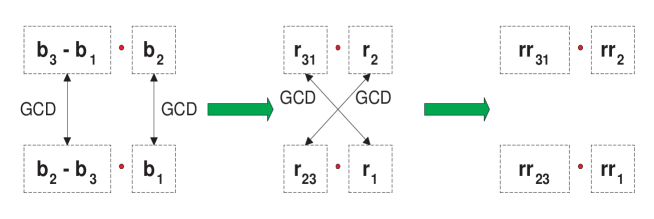
  Figure 1: Bringing a product of two fractions to complete irreducibility without multiplying.

  We still do not perform multiplications for fear of an overflow. But now it is evident that a solution can only exist if $rr_{23}\leq n_{1},\quad rr_{1}\leq n_{1},\quad rr_{31}\leq n_{2},\quad rr_{2}\leq n_{2}$. We first check these inequalities; if one or more of them do not hold, we proceed with the $n$-cycle, otherwise we may safely perform multiplications (both products do not exceed $D^{2}$) and look for solutions.

2.4 Example 2: drift waves in a channel

The turbulence of the drift waves is described by the same equation as in Sec.2.1 but in Descartes coordinates and in the infinite channel[7]. In this case dispersion function has a (slightly simplified) form $\omega=2m/(n^{2}+1)$ and resonance conditions are

$$\begin{cases}\omega_{1}+\omega_{2}=\omega_{3}\\ m_{1}+m_{2}=m_{3}\\ m_{i}\leq n_{i}\quad\forall i=1,2,3\\ n_{i}\neq n_{j}\quad\forall i\neq j\\ \end{cases}$$ (13)

Search cycles on $n_{1}$, $n_{2}$, $n_{3}$ become somewhat more extensive due to the lack of the two conditions mentioned above. On the other hand, the core of the algorithm - the four reductions (Step 2) - are preserved one-to-one, as well as the post-reduction overflow check (Step 3).

The computational complexity of the whole algorithm is also $O(\log DD^{3})$ as in the previous case.

3 Numerical results and some discussion

Our algorithm has been implemented in VBA programming language; for $D=1000$ computation time (without disk output of solutions found) on a low-end PC (800 MHz Pentium III, 512 MB RAM) is about 7.5 minutes. Altogether 7282 solutions (example 1) have been found. Some overall numerical data is given in the Tables and Figures below.

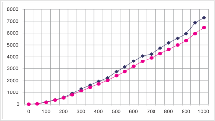
Figure 2: Example 1: Number of all solutions in partial domains: squares (points with diamonds) and circles (points with circles).

In Fig.2 the number of solutions in partial domains is shown for the first example (atmospheric planetary waves) and we conclude that the solutions are concentrated along $X$ and $Y$ axes. In Fig.3 the histogram of vector multiplicities is presented which shows in how many solutions one vector can participate. On the axis $X$ the multiplicity of a vector is shown and on the axis $Y$ the number of vectors with a given multiplicity. One can see immediately that most part of vectors take part only in one solution and multiplicity decreases exponentially with the number of solutions.

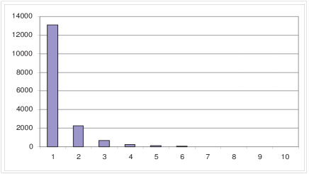
Figure 3: Example 1: Histogram of vector multiplicities.

As to our second example (drift waves in a channel) we notice, first of all, much less solutions ($477$) in the same main domain $D=1000$. Therefore, not much can be said about the asymptotic of solution number in partial domains. There is no need to present multiplicities graphically in this case. In the whole calculation domain $D=1000$ there is just one vector $(1,5)$ participating in solutions with multiplicity $5$, one vector $(78,99)$ with multiplicity $4$ and the overall distribution is as follows:

Multiplicity	1	2	3	4	5
Number of vectors	1254	72	8	1	1

Table 1. Example 2: Vector multiplicities.

In order to understand the energetic behavior of 2-dimensional discrete wave system, the standard way is to present is graphically on the integer lattice in following way. Each node with coordinates $m,n$ presents a corresponding wave vector $\vec{k}=(m,n)$ and nodes-vectors are connected by lines is they are parts of the same solution. An example of this geometrical structure is given in Fig.4.

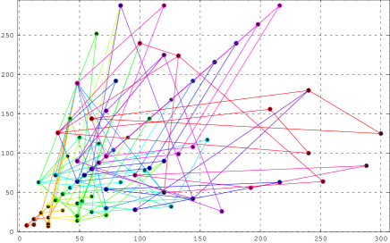
Figure 4: Example of geometrical structure of a solution set.

This geometrical representation is needed in order to understand what sort of equations (ODEs) for the amplitudes of resonantly interacting waves we have to solve. Namely, one single triangle in $\vec{k}$-space corresponds to

$$\begin{cases}\dot{A}_{1}=\alpha_{1}A_{2}A_{3}\\ \dot{A}_{2}=\alpha_{2}A_{1}A_{3}\\ \dot{A}_{3}=\alpha_{3}A_{1}A_{2}\end{cases}$$ (14)

where coefficients $\alpha_{i}$ are known functions on $m_{i},n_{i},\ i=1,2,3$. If one wave takes part in two solutions, we get two systems of this form connected via this wave, for instance, if the second solution corresponds to

$$\dot{A}_{4}=\alpha_{4}A_{5}A_{6},\quad\dot{A}_{5}=\alpha_{5}A_{4}A_{6},\quad\dot{A}_{6}=\alpha_{6}A_{4}A_{4},$$

and they are connected via one wave, say $A_{3}=A_{4}$, then corresponding system of ODEs takes form

$$\begin{cases}\dot{A}_{1}=\alpha_{1}A_{2}A_{3}\\ \dot{A}_{2}=\alpha_{2}A_{1}A_{3}\\ \dot{A}_{3}=\frac{1}{2}(\alpha_{3}A_{1}A_{2}+\alpha_{4}A_{5}A_{6})\\ \dot{A}_{5}=\alpha_{5}A_{3}A_{6}\\ \dot{A}_{6}=\alpha_{6}A_{3}A_{5}\end{cases}$$ (15)

and so on.

Obviously, the geometrical structure is too confusing to be informative and what we really need is a topological structure of a solution set, i.e. the graph formed by triangles as primary elements. Namely, it is enough to compute all non-isomorphic topological elements because all isomorphic elements are described by the same system of ODEs. For instance, all primary elements (isolated resonant triads) are described by (14), all ”butterflies” (groups of two connected triads) are described by (15), etc. The difference between two isomorphic topological elements lies in the coefficients $\alpha_{i}$ which are functions of the wave numbers, and therefore, will take different magnitudes for different resonant triads. Topological structure of the solution set for our first example is shown in Fig. 5 for domain $m,n\leq 50.$ This domain contains 42 solutions: 15 isolated triangles, two ”butterflies” (groups of two connected triangles), one chain of three connected triangles and two more complex graphs.

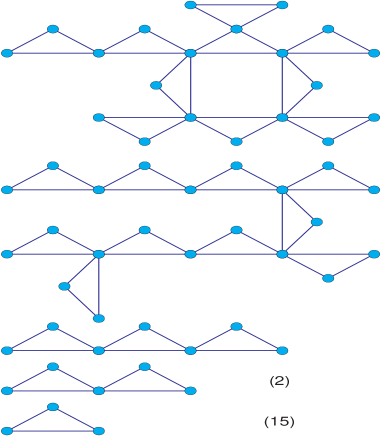
Figure 5: Example 1: Topological structure of solutions for $D=50$.

4 Summary

This paper concludes the series of three papers on generic algorithms for laminated wave turbulence. We have presented algorithms for polynomial dispersion function depending irrationally on the wave vector length $k=\sqrt{m^{2}+n^{2}}$ and for an arbitrary rational dispersion function. We have also shown that the topological elements of the solution set (for the discrete layer of turbulence) give the whole information about the energy transport in these wave systems. In fact we applied this approach for our first example (atmospheric planetary waves) and studied all the topological elements in the meteorologically significant domain ($m,n\leq 21$) for climate range processes[8]. More precisely, we have found analytically solutions of corresponding systems of the form (14) in terms of Jacobean elliptic functions and computed their periods and other properties for characteristic meteorological data. As a result, a novel model of the known physical phenomena - intra-seasonal oscillations in the Earth atmosphere - has been developed.

Our further interest lies now in the area of symbolic computations. Indeed, beginning with an equation like (5) with given boundary conditions, we have a completely constructive procedure of obtaining precise form for: I) resonance conditions (1); II) coefficients $\alpha_{i}$ of the primary element (14); III) all topological elements - as graphs and as corresponding systems of ODEs. All this can be programmed symbolically in MATHEMATICA and solutions can be found using our generic algorithms. This is an on-going work now and we plan to create a useful program tool for making basic research in the area of discrete wave turbulence. There are some open mathematical questions yet to be solved - for instance, the problem of graph isomorphism appearing at the step when all different topological elements have to be computed.

Another possible development would be the study of the 4-wave interactions, that is, with primary elements being not triads but quartets of waves (see example of gravitational water waves[4],[5]). The same constructive procedure as for 3-wave interactions can be applied but the resulting topology will be much more complicated due to the principal difference between 3- and 4-wave systems. In 3-wave system there exist the only mechanism for the energy transport - transport over the scales. In 4-wave system there are two qualitatively different mechanisms of the energy flow - over the scales and over the phases, and they can combine in a highly nontrivial way.

Acknowledgement. E.K. acknowledges the support of the Austrian Science Foundation (FWF) under projects SFB F013/F1304.

References

- [1] V.E. Zakharov, V.S. L’vov, G. Falkovich. Kolmogorov Spectra of Turbulence (Series in Nonlinear Dynamics, Springer, 1992)
- [2] E.A. Kartashova. PRL (72), 2013 (1994); E.A. Kartashova. AMS Transl. (182), 2, 95 (1998) and others
- [3] E.A. Kartashova. JETP Letters (83) 7, 341 (2006)
- [4] E. Kartashova, A. Kartashov. IJMPC 17(11), 1579 (2006)
- [5] E. Kartashova, A. Kartashov. CiCP, to appear (2006)
- [6] J. Pedlosky. Geophysical Fluid Dynamics (Second Edition, Springer, 1987)
- [7] A.M. Balk, S.V. Nazarenko, V.E. Zakharov. Phys. Letters A (152), 5-6, 280 (1991)
- [8] E. Kartashova, V. L’vov. E-print arXiv.org:nlin/0606058. Submitted (a shortened version) to PRL (2006)