A probabilistic approach to Zhang’s sandpile model

Abstract

The current literature on sandpile models mainly deals with the abelian sandpile model (ASM) and its variants. We treat a less known - but equally interesting - model, namely Zhang’s sandpile. This model differs in two aspects from the ASM. First, additions are not discrete, but random amounts with a uniform distribution on an interval $[a,b]$. Second, if a site topples - which happens if the amount at that site is larger than a threshold value $E_{c}$ (which is a model parameter), then it divides its entire content in equal amounts among its neighbors. Zhang conjectured that in the infinite volume limit, this model tends to behave like the ASM in the sense that the stationary measure for the system in large volumes tends to be peaked narrowly around a finite set. This belief is supported by simulations, but so far not by analytical investigations.

We study the stationary distribution of this model in one dimension, for several values of $a$ and $b$. When there is only one site, exact computations are possible. Our main result concerns the limit as the number of sites tends to infinity, in the one-dimensional case. We find that the stationary distribution, in the case $a\geq E_{c}/2$, indeed tends to that of the ASM (up to a scaling factor), in agreement with Zhang’s conjecture. For the case $a=0$, $b=1$ we provide strong evidence that the stationary expectation tends to $\sqrt{1/2}$.

1 Introduction and main results

With the introduction of the sandpile model by Bak, Tang and Wiesenfeld (BTW), the notion of self-organized criticality was introduced, and subsequently applied to several other models such as forest-fire models, and the Bak-Sneppen model for evolution. In turn, these models serve as a paradigm for a variety of natural phenomena in which, empirically, power laws of avalanche characteristics and/or correlations are found, such as the Gutenberg-Richter law for earthquakes. See [12] for a extended overview.

After the work of Dhar [2], the BTW model was later renamed ‘abelian sandpile model’ (ASM), referring to the abelian group structure of addition operators. This abelianness has since served as the main tool of analysis for this model.

A less known variant of the BTW-model has been introduced by Zhang [13], where instead of discrete sand grains, continuous height variables are used. This lattice model is described informally as follows. Consider a finite subset $\Lambda\subset\mathbb{Z}^{d}$. Initially, every lattice site $i\in\Lambda$ is given an energy $0\leq E_{i}<E_{c}$, where $E_{c}$ is the so called critical threshold, and often chosen to be equal to 1. Then, at each discrete time step, one adds a random amount of energy, uniformly distributed on some interval $[a,b]\subset[0,E_{c}]$, at a randomly chosen lattice site. If the resulting energy at this site is still below the critical value then we have arrived at the new configuration. If not, an avalanche is started, in which all unstable sites (that is, sites with energy at least $E_{c}$) ‘topple’ in parallel, i.e., give a fraction $1/2d$ of their energy to each neighbor in $\Lambda$. As usual in sandpile models, upon toppling of boundary sites, energy is lost. As in the BTW-model, the stabilization of an unstable configuration is performed instantaneously, i.e., one only looks at the final stable result of the random addition.

In his original paper, Zhang observes, based on results of numerical simulation (see also [6]), that for large lattices, the energy variables in the stationary state tend to concentrate around discrete values of energy; he calls this the emergence of energy ‘quasi-units’. Therefore, he argues that in the thermodynamic limit, the stationary dynamics should behave as in the discrete ASM. However, Zhang’s model is not abelian (the next configuration depends on the order of topplings in each avalanche; see below), and thus represents a challenge from the analytical point of view. There is no mentioning of this fact in [6, 13], see however [8]; probably they chose the usual parallel order of topplings in simulations.

After its introduction, a model of Zhang’s type (the toppling rule is the same as Zhang’s, but the addition is a deterministic amount larger than the critical energy) has been studied further in the language of dynamical systems theory in [1]. The stationary distributions found for this model concentrate on fractal sets. Furthermore, in these studies, emergence of self-organized criticality is linked to the behavior of the smallest Lyapounov exponents for large system sizes. From the dynamical systems point of view, Zhang’s model is a non-trivial example of an iterated function system, or of a coupled map lattice with strong coupling.

In this paper we rigorously study Zhang’s model in dimension $d=1$ with probabilistic techniques, investigating uniqueness and deriving certain properties of the stationary distribution. Without loss of generality, we take $E_{c}=1$ throughout the paper. In Section 2 we rigorously define the model for $d=1$. We show that in the particular case of $d=1$ and stabilizing after every addition, the topplings are in fact abelian, so that the model can be defined without specifying the order of topplings. In that section, we also include a number of general properties of stationary distributions. For instance, we prove that if the number of sites is finite, then every stationary distribution is absolutely continuous with respect to Lebesgue measure on $(0,1)$, in contrast with the fractal distributions for the model defined in [1] (where the additions are deterministic).

We then study several specific cases of Zhang’s model. For each case, we prove by coupling that the stationary distribution is unique. In Section 4, we explicitly compute the stationary distribution for the model on one site, with $a=0$, by reducing it to the solution of a delay equation [3].

Our main result is in Section 5, for the model with $a\geq 1/2$. We show that in the infinite volume limit, every one-site marginal of the stationary distribution concentrates on a non-random value, which is the expectation of the addition distribution (Theorem 5.5). This supports Zhang’s conjecture that in the infinite volume limit, his model tends to behave like the abelian sandpile. Section 5 contains a number of technical results necessary for proving Theorem 5.5, but which are also of independent interest. For instance, we construct a coupling of the so-called reduction of Zhang’s model to the abelian sandpile model, and we prove that any initial distribution converges exponentially fast to the stationary distribution.

In Section 6, we treat the model for $[a,b]=[0,1]$. We present simulations that indicate the emergence of quasi-units also for this case. However, since in this case there is less correspondence with the abelian sandpile model, we cannot fully prove this. We can prove that the stationary distribution is unique, and we show that if every one-site marginal of the stationary distribution tends to the same value in the infinite volume limit, and in addition if there is a certain amount of asymptotic independence, then this value is $\sqrt{1/2}$. This value is consistent with our own simulations.

2 Model definition

We define Zhang’s model in dimension one as a discrete-time Markov process with state space $\Omega_{N}:=[0,1)^{\{1,2,\ldots,N\}}\subset[0,\infty)^{\{1,2,\ldots,N\}}:=\Xi_{N}$, endowed with the usual sigma-algebra. We write $\eta,\xi\in\Omega_{N}$, configurations of Zhang’s model and $\eta_{j}$ for the $j$th coordinate of $\eta$. We interpret $\eta_{j}$ as the amount of energy at site $j$.

By ${\mathbb{P}}_{\eta}$, we denote the probability measure on (the usual sigma-algebra on) the path space $\Omega_{N}^{\mathbb{N}}$ for the process started in $\eta$. Likewise we use ${\mathbb{P}}_{\nu}$ when the process is started from a probability measure $\nu$ on $\Omega_{N}$, that is, with initial configuration chosen according to $\nu$. The configuration at time $t$ is denoted as $\eta(t)$ and its $j$th component as $\eta_{j}(t)$.

We next describe the evolution of the process. Let $0\leq a<b\leq 1$. At time 0 the process starts in some configuration $\eta\in\Omega_{N}$. For every $t=1,2,\ldots$, the configuration $\eta(t)$ is obtained from $\eta(t-1)$ as follows. At time $t$, a random amount of energy $U_{t}$, uniformly distributed on $[a,b]$, is added to a uniformly chosen site $X_{t}\in\{1,\ldots,N\}$, hence $P(X_{t}=j)=1/N$ for all $j=1,\ldots,N$. We assume that $U_{t}$ and $X_{t}$ are independent of each other and of the past of the process. If, after the addition, the energies at all sites are still smaller than 1, then the resulting configuration is in $\Omega_{N}$ and this is the new configuration of the process.

If however after the addition the energy of site $X_{t}$ is at least 1 - such a site is called unstable - then this site will topple, i.e., transfer half of its energy to its left neighbor and the other half to its right neighbor. In case of a toppling of a boundary site, this means that half of the energy disappears. The resulting configuration after one toppling may still not be in $\Omega_{N}$, because a toppling may give rise to other unstable sites. Toppling continues until all sites have energy smaller than 1 (i.e., until all sites are stable). This final result of the addition is the new configuration of the process in $\Omega_{N}$. The entire sequence of topplings after one addition is called an avalanche.

We call the above model the $(N,[a,b])$-model. We use the symbol $\mathcal{T}_{x}(\xi)$ for the result of toppling of site $x$ in configuration $\xi\in\Xi_{N}$. We write $\mathcal{A}_{u,x}(\eta)$ for the result of adding an amount $u$ at site $x$ of $\eta$, and stabilizing through topplings.

It is not a priori clear that the process described above is well defined. By this we mean that it is not a priori clear that every order in which we perform the various topplings leads to the same final configuration $\eta(t)$. In fact, unlike in the abelian sandpile, topplings according to Zhang’s toppling rule are not abelian in general. To give an example of non-abelian behavior, let $N=2$ and $\xi=(1.2,1.6)$. Then $\mathcal{T}_{1}(\mathcal{T}_{2}(\xi))=\mathcal{T}_{1}((2,0))=(0,1)$, whereas $\mathcal{T}_{2}(\mathcal{T}_{1}(\xi))=\mathcal{T}_{2}((0,2.2))=(1.1,0)$.

Despite this non-abelianness of certain topplings, we will now show that in the process defined above, we only encounter avalanches that consist of topplings with the abelian property. When restricted to a certain subset of $\Omega_{N}$, topplings are abelian, and it turns out that this subset is all we use. (In particular, the example that we just gave cannot occur in our process.)

Proposition 2.1.

The $(N,[a,b])$-model is well defined.

Proof.

We will prove in two steps that all topplings actually encountered in the process are abelian. To this end, we first show that in Zhang’s model in dimension one, we can never create two adjacent unstable sites by making one addition to a stable configuration and toppling unstable sites in any order.

Let $\tilde{\Omega}_{N}\subset\Xi_{N}$ be the set of all (possibly unstable) configurations such that between every pair of unstable sites there is at least one empty site, and such that the energy of any unstable site is smaller than 2. It is clear that by making an addition to a stable configuration, we arrive in $\tilde{\Omega}_{N}$. We show that, for every configuration $\tilde{\eta}\in\tilde{\Omega}_{N}$, the resulting configuration after toppling of one of the unstable sites is still in $\tilde{\Omega}_{N}$. Introducing some notation, we call a site $j$ of a configuration $\eta$

$$\begin{array}[]{lll}\textrm{empty}&\textrm{if}&\eta_{j}=0,\\ \textrm{nonempty}&\textrm{if}&\eta_{j}\in(0,1),\\ \textrm{unstable}&\textrm{if}&\eta_{j}\geq 1.\\ \end{array}$$

An unstable site $i$ of $\tilde{\eta}$ can have either two empty neighbors (first case), two nonempty neighbors (second case) or one nonempty and one empty (third case).

In the first case, toppling of site $i$ cannot create a new unstable site, since $\frac{1}{2}\tilde{\eta}_{i}<1$, but $i$ itself becomes empty. Thus, if there were unstable sites to the left and to the right of $i$, after the toppling there still is an empty site between them.

In the second and third case, the nonempty neighbor(s) of $i$ can become unstable. Suppose the left neighbor $i-1$ becomes unstable. Directly to its right, at $i$, an empty site is created. To its left, there was either no unstable site, or first an empty site and then somewhere an unstable site. The empty site can not have been site $i-1$ itself, because to have become unstable it must have been nonempty. For the right neighbor the same argument applies. Therefore, the new configuration is still in $\tilde{\Omega}_{N}$.

So far, we showed that in the process of stabilization after addition to a stable configuration, only configurations in $\tilde{\Omega}_{N}$ are created. In the second step of the proof we show that, if $\eta\in\tilde{\Omega}_{N}$ and $i$ and $j$ are unstable sites in $\eta$, then

$$\mathcal{T}_{i}(\mathcal{T}_{j}(\eta))=\mathcal{T}_{j}(\mathcal{T}_{i}(\eta)).$$ (1)

To prove this, we consider all different possibilities for $x$. If $x$ is not a neighbor of either $i$ or $j$, then toppling of $i$ or $j$ does not change $\eta_{x}$, so that (1) is obvious. If $x$ is equal to $i$ or $j$, or neighbor to only one of them, then only one of the topplings changes $\eta_{x}$, so that again (1) is obvious. Finally, if $x$ is a neighbor of both $i$ and $j$, then, since $\eta\in\tilde{\Omega}_{N}$, $x$ must be empty before the topplings at $i$ and $j$. We then have

$$\mathcal{T}_{j}(\eta)_{x}=\frac{1}{2}\eta_{j},$$

so that

$$\mathcal{T}_{i}(\mathcal{T}_{j}(\eta))_{x}=\frac{1}{2}\eta_{j}+\frac{1}{2}\eta_{i}=\mathcal{T}_{j}(\mathcal{T}_{i}(\eta))_{x}$$

Therefore, also in this last case (1) is true.

Having established that the topplings of two unstable sites commute, it follows that the final stable result after an addition is independent of the order in which we topple, and hence $\mathcal{A}_{u,x}(\eta(t))$ is well-defined; see [7], Section 2.3 for a proof of this latter fact. ∎

Remark 2.2.

It will be convenient to order the topplings in so-called waves [9]. Suppose the addition of energy at time $t$ takes place at site $k$ and makes this site unstable. In the first wave, we topple site $k$ and then all other sites that become unstable, but we do not topple site $k$ again. After this wave only site $k$ can possibly be unstable. If site $k$ is unstable after this first wave, the second wave starts with toppling site $k$ (for the second time) and then all other sites that become unstable, leaving site $k$ alone, until we reach a configuration in which all sites are stable. This is the state of the process at time $t$. It is easy to see that in each wave, every site can topple at most once.

3 Preliminaries and technicalities

In this section, we discuss a number of technical results which are needed in the sequal, and which are also interesting in their own right. The section is subdivided into three subsections, dealing with connections to the abelian sandpile, avalanches, and nonsingularity of the marginals of stationary distributions, respectively.

3.1 Comparison with the abelian sandpile model

We start by giving some background on the abelian sandpile model in one dimension. In the abelian sandpile model on a finite set $\Lambda\subset\mathbb{Z}$, the amount of energy added is a nonrandom quantity: each time step one grain of sand is added to a random site. When a site is unstable, i.e., it contains at least two grains, it topples by transferring one grain of sand to each of its two neighbors (at the boundary grains are lost). The abelian addition operator is as follows: add a particle at site $x$ and stabilize by toppling unstable sites, in any order. We denote this operator by $a_{x}:\{0,1\}^{\Lambda}\to\{0,1\}^{\Lambda}$. For toppling of site $x$ in the abelian sandpile model, we use the symbol $T_{x}$. Abelian sandpiles have some convenient properties [2]: topplings on different sites commute, addition operators commute, and the stationary measure on finitely many sites is the uniform measure on the set of so-called recurrent configurations. Recurrent (or allowed) configurations are characterized by the fact that they do not contain a forbidden subconfiguration (FSC). A FSC is defined as a restriction of $\eta$ to a subset $W$ of $\Lambda$, such that $\eta_{x}$ is less than the number of neighbors of $x$ in $W$, for all $x$. In [9], a proof can be found that a FSC cannot be created by an addition or by a toppling.

In the one-dimensional case on $N$ sites, the abelian sandpile model behaves as follows. Sites are either empty, containing no grains, or full, containing one grain. When an empty site receives a grain, it becomes full, and when a full site receives a grain, it becomes unstable. In the latter case, the configuration changes in the following manner. Suppose the addition site was $x$. We call the distance to the first site that is empty to the left $i$. If there is no empty site to the left, then $i-1$ is the distance to the boundary. $j$ is defined similarly, but now to the right. After stabilization, the sites in $\{x-i,\ldots,x+j\}\cap\{1,\ldots,N\}$ are full, except for a new empty site at $x-i+j$. Only sites in $\{x-i,\ldots,x+j\}\cap\{1,\ldots,N\}$ have toppled. The amount of topplings of each site is equal to the minimum of its distances to the endsites of the avalanche. For example, boundary sites can never topple more than once in an avalanche. These results follow straightforwardly from working out the avalanche.

The recurrent configurations are those with at most one empty site; a FSC in the one-dimensional case is a subset of $\Lambda$ of more than 1one site, with empty sites at its boundary.

Here is an example of how a non-recurrent state on 11 sites relaxes through topplings. An addition was made to the 7th site; underlined sites are the sites that topple. The topplings are ordered into waves (see Remark 2.2). In the example, the second wave starts on the 5th configuration:

$$110111\underline{2}1101 \to 11011\underline{2}0\underline{2}101\to 1101\underline{2}020\underline{2}01\to 110\underline{2}0121011\to 111011\underline{2}1011$$

$$\to 11101\underline{2}0\underline{2}011\to 1110\underline{2}020111\to 111101\underline{2}0111\to 11110\underline{2}01111$$

$$\to 11111011111.$$

To compare Zhang’s model to the abelian sandpile, we label the different states of a site $j\in\{1,\ldots,N\}$ in $\eta\in\tilde{\Omega}_{N}$ as follows:

$$\begin{array}[]{lll}\textrm{empty}(0)&\textrm{if}&\eta_{j}=0,\\ \textrm{full}(1)&\textrm{if}&\eta_{j}\in[\frac{1}{2},1),\\ \textrm{unstable}(2)&\textrm{if}&\eta_{j}\geq 1,\\ \textrm{anomalous}(a)&\textrm{if}&\eta_{j}\in(0,\frac{1}{2}).\\ \end{array}$$ (2)

Definition 3.1.

The reduction of a configuration $\eta\in\tilde{\Omega}_{N}$ is the configuration denoted by $\mathcal{R}(\eta)\in\{0,1,2,a\}^{\{1,\ldots,N\}}$ corresponding to $\eta$ by (2).

For general $0\leq a<b\leq 1$, we have the following result.

Proposition 3.2.

For any starting configuration $\eta\in\Omega$, there exists a random variable $T\geq 0$ with $P(T<\infty)=1$ such that for all $t\geq T$, $\eta(t)$ contains at most one empty or anomalous site. Moreover, for $t\geq T$, given that $\eta(t)$ contains an empty site $x_{t}$, the distribution of this site is uniform on $\{1,\ldots,N\}$.

To prove this proposition, we first introduce FSC’s for Zhang’s model. We define a FSC in Zhang’s model in one dimension as the restriction of $\eta$ to a subset $W$ of $\{1,\ldots,N\}$, in such a way that $2\eta_{j}$ is less than the number of neighbors of $j$ in $W$, for all $j\in W$. From here on, we will denote the number of neighbors of $j$ in $W$ by $\mbox{deg}_{W}(j)$. To distinguish between the two models, we will from now on call the above Zhang-FSC, and the definition given in Section 3.1 abelian-FSC. From the definition, it follows that a Zhang-FSC in a stable configuration is a restriction to a subset of more than one site, with the boundary sites either empty or anomalous. Note that according to this definition, a stable configuration without Zhang-FSC’s can be equivalently described as a configuration with at most one empty or anomalous site.

Lemma 3.3.

A Zhang-FSC cannot be created by an addition in Zhang’s model.

Proof.

The proof is similar to the proof of the corresponding fact for abelian-FSC’s, which can be found for instance in [7], Section 5. We suppose that $\eta(t)$ does not contain an FSC, and an addition was made at site $x$. If the addition caused no toppling, then it cannot create a Zhang-FSC, because no site decreased its energy. Suppose therefore that the addition caused a toppling in $x$. Then for each neighbor $y$ of $x$

$$\mathcal{T}_{x}(\eta)_{y}\geq\eta_{y}+\frac{1}{2},$$

so that $2\mathcal{T}_{x}(\eta)_{y}\geq 2\eta_{y}+1$. Also $\mathcal{T}_{x}(\eta)_{x}=0$, and all other sites are unchanged by the toppling.

We will now derive a contradiction. Suppose the toppling created a Zhang-FSC, on a subset which we call $W$. It is clear that this means that $x$ should be in $W$, because it is the only site that decreased its energy by the toppling. For all $j\in W$, we should have that $2\mathcal{T}_{x}(\eta)_{j}<\mbox{deg}_{W}(j)$. This means that for all neighbors $y$ of $x$ in $W$, we have $2\eta_{y}<\mbox{deg}_{W}(y)-1$, and for all other $j\in W$ we have $2\eta_{j}<\mbox{deg}_{W}(j)$. From these inequalities it follows that $W\setminus\{x\}$ was already a Zhang-FSC before the toppling, which is not possible, because we supposed that $\eta(t)$ contained no Zhang-FSC.

By the same argument, further topplings cannot create a Zhang-FSC either, and the proof is complete. ∎

Remark 3.4.

We have not defined Zhang’s model in dimension $d>1$, because in that case the resulting configuration of stabilization through topplings is not independent of the order of topplings. But since the proof above only discusses the result of one toppling, Lemma 3.3 remains valid for any choice of order of topplings. The proof is extended simply by replacing the factor 2 by $2d$.

Proof of Proposition 3.2. If $\eta$ already contains at most one non-full, i.e., empty or anomalous site, then it contains no Zhang-FSC’s, and the proposition follows. Suppose therefore that at some time $t$, $\eta(t)$ contains $M(t)$ non-full sites, with $1<M(t)\leq N$. We denote the positions of the non-full sites of $\eta(t)$ by $Y_{i}(t)$, $i=1,\ldots,M(t)$, and we will show that $M(t)$ is nonincreasing in $t$, and decreases to 1 in finite time. Note that for all $1\leq i<j\leq M(t)$, the restriction of $\eta(t)$ to $\{Y_{i}(t),Y_{i}(t)+1,\ldots,Y_{j}(t)\}$ is a Zhang-FSC.

At time $t+1$, we have the following two possibilities. Either the addition causes no avalanche, in that case $M(t+1)\leq M(t)$, or it causes an avalanche. We will call the set of sites that change in an avalanche (that is, all sites that topple at least once, together with their neighbors) the range of the avalanche. We first show that if the range at time $t+1$ contains a site $y\in\{Y_{i}(t),\ldots,Y_{i+1}(t)\}$ for some $i$, then $M(t+1)<M(t)$.

Suppose there is such a site. Then, since $\{Y_{i}(t)+1,\ldots,Y_{i+1}(t)-1\}$ contains only full sites, all sites in this subset will topple and after stabilization of this subset, it will not contain a Zhang-FSC. In other words, in this subset at most one non-full site is created. But since $Y_{i}(t)$ and $Y_{i+1}(t)$ received energy from a toppling neighbor, they are no longer empty or anomalous. Therefore, $M(t+1)<M(t)$.

If there is no such site, then the range is either $\{1,Y_{1}(t)\}$, or $\{Y_{M(t)}(t),N\}$. With the same reasoning as above, we can conclude that in these cases, $Y_{1}(t+1)<Y_{1}(t)$, resp. $Y_{M(t)}(t+1)>Y_{M(t)}(t)$.

Thus, $M(t)$ strictly decreases at every time step where an avalanche contains topplings between two non-full sites. As long as there are at least two non-full sites, such an avalanche must occur eventually. We cannot make infinitely many additions without causing topplings, and we cannot infinitely many times cause an avalanche at $x<Y_{1}(t)$ or $x>Y_{M(t)}(t)$ without decreasing $M(t)$, since after each such an avalanche, these non-full sites ‘move’ closer to the boundary. ∎

In the case that $a\geq 1/2$, we can further specify some characteristics of the model. We prove that for any initial configuration, after at most $N(N-1)$ time steps there is at most one empty site, and the other sites are is full, i.e., there are no anomalous sites. We will call such configurations regular.

Proposition 3.5.

Suppose $a\geq\frac{1}{2}$. Then

1. for any initial configuration $\eta$, for all $t\geq N(N-1)$, $\eta(t)$ is regular,

2. for every stationary distribution $\mu$, and for all $i\in\{1,\ldots,N\}$,

   $$\mu(\eta_{i}=0)=\frac{1}{N+1}.$$

In words, this proposition states that if $a\geq 1/2$, then every stationary distribution concentrates on regular configurations. Moreover, the stationary probability that a certain site $i$ is empty, does not depend on $i$. Note that as a consequence, the stationary probability that all sites are full, is also $\frac{1}{N+1}$.

To prove this proposition, we need the following lemma. In words, it states that if $a\geq 1/2$ and $\eta$ contains no anomalous sites, then the reduction of Zhang’s model (according to Definition 3.1) behaves just as the abelian sandpile model.

Lemma 3.6.

For all $u\in[\frac{1}{2},1)$, for all $\eta\in\Omega_{N}$ which do not contain anomalous sites, and for all $x\in\{1,\ldots,N\}$

$$\mathcal{R}(\mathcal{A}_{u,x}(\eta))=a_{x}(\mathcal{R}(\eta)),$$ (3)

where $a_{x}$ is the addition operator of the abelian sandpile model. In both avalanches, corresponding sites topple the same number of times.

Proof.

Under the conditions of the lemma, site $x$ can be either full or empty. If $x$ is empty, then upon the addition of $u\geq\frac{1}{2}$ it becomes full. No topplings follow, so that in that case we directly have $\mathcal{R}(\mathcal{A}_{u,x}(\eta))=a_{x}(\mathcal{R}(\eta))$.

If $\eta$ is such that site $x$ is full, then upon addition it becomes unstable. We call the configuration after addition, but before any topplings $\tilde{\eta}$. To check if in that case $\mathcal{R}(\mathcal{A}_{u,x}(\eta))=a_{x}(\mathcal{R}(\eta))$, we only need to prove $\mathcal{R}(\mathcal{T}_{x}(\tilde{\eta}))=T_{x}(\mathcal{R}(\tilde{\eta}))$, with $\mathcal{R}(\tilde{\eta})_{x}=2$, since we already know that in both models, the final configuration after one addition is independent of the order of topplings.

In $\mathcal{T}_{x}(\tilde{\eta})$, site $x$ will be empty. This corresponds to the abelian toppling, because site $x$ contained two grains after the addition, and by toppling it gave one to each neighbor. In $\mathcal{T}_{x}(\tilde{\eta})$, the energy of the neighbors of $x$ is their energy in $\eta$, plus at least $\frac{1}{2}$. Thus the neighbors of site $x$ will in $\mathcal{T}_{x}(\tilde{\eta})$ be full if they were empty, or unstable if they were full. Both correspond to the abelian toppling, where the neighbors of $x$ received one grain. ∎

Proof of Proposition 3.5. To prove part (1), we note that any amount of energy that a site can receive during the process, i.e., either an addition or half the content of an unstable neighbor, is at least $1/2$. Thus, anomalous sites can not be created in the process. Anomalous sites can however disappear, either by receiving an addition, or, as we have seen in the proof of Proposition 3.2, when they are in the range of an avalanche.

When we make an addition of at least $1/2$ to a configuration with more than one non-full site, then either the number of non-full sites strictly decreases, or one of the outer non-full sites moves at least one step closer to the boundary. We note that $\eta$ contains at most $N$ non-full sites, and the distance to the boundary is at most $N-1$. When finally there is only one non-full site, then in the next time step it must either become full or be in the range of an avalanche. Thus, there is a random time $T^{\prime}\leq N(N-1)$ such that $\eta(T^{\prime})$ is regular for the first time, and as anomalous sites cannot be created, by Proposition 3.2, $\eta(t)$ is regular for all $t\geq T^{\prime}$.

For $t\geq T^{\prime}$, $\eta(t)$ satisfies the condition of Lemma 3.6. This means that the stationary distribution of the reduction of Zhang’s model must coincide with that of the abelian sandpile model. As we mentioned in Section 3.1, this is the uniform measure on all configurations with at most one empty site. This proves part (2). ∎

3.2 Avalanches in Zhang’s model

We next describe in full detail the effect of an avalanche, started by an addition to a configuration $\eta(t)$ in Zhang’s model. Let $\mathcal{C}(t+1)$ be the range of this avalanche. Recall that we defined the range of an avalanche as the set of sites that change their energy at least once in the course of the avalanche (that is, all sites that topple at least once, together with their neighbors). We denote by $\mathcal{T}(t+1)$ the collection of sites that topple at least once in the avalanche. Finally, $\mathcal{C}^{\prime}(t+1)\subset\mathcal{C}(t+1)$ denotes the collection of anomalous sites that change, but do not topple in the avalanche.

During the avalanche, the energies of sites in the range, as well as $U_{t+1}$, get redistributed through topplings in a rather complicated manner. By decomposing the avalanche into waves (see Remark 2.2), we prove the following properties of this redistribution.

Proposition 3.7.

Suppose an avalanche is started by an addition at site $x$ to configuration $\eta(t)$. For all sites $j$ in $\mathcal{C}(t+1)$, there exist $F_{ij}=F_{ij}(\eta(t),x,U_{t+1})$ such that we can write

$$\eta_{j}(t+1)=\sum_{i\in\mathcal{T}(t+1)}F_{ij}\eta_{i}(t)+F_{xj}U_{t+1}+\eta_{j}(t){\large\bf{1}}_{j\in\mathcal{C}^{\prime}(t+1)},$$ (4)

with

1. $$F_{xj}+\sum_{i\in\mathcal{T}(t+1)}F_{ij}=\mathcal{R}(\eta(t+1))_{j};$$ (5)

2. for all $j\in\mathcal{C}(t+1)$ such that $\eta_{j}(t+1)\neq 0$,

   $$F_{xj}\geq 2^{-\lceil 3N/2\rceil};$$

3. for all $j\in\mathcal{C}(t+1)$ such that $\eta_{j}(t+1)\neq 0$, $j\geq x$, we have

   $$F_{x,j+1}\leq F_{xj};$$

   and similarly, $F_{x,j-1}\leq F_{xj}$ for $j\leq x$.

In words, we can write the new energy of each site in the range of the avalanche at time $t+1$ as a linear combination of energies at time $t$ and the addition $U_{t+1}$, in such a way that the prefactors sum up to 1 or 0. Furthermore, every site in the range receives a positive fraction of at least $2^{-\lceil 3N/2\rceil}$ of the addition. These received fractions are such that larger fractions are found closer to the addition site. We will need this last property in the proof of Theorem 5.5.

Proof of Proposition 3.7. We start with part (1). First, we decompose the avalanche started at site $x$ into waves. We index the waves with $k=1,\ldots,K$, and write out explicitly the configuration after wave $k$, in terms of the configuration after wave $k-1$. The energy of site $i$ after wave $k$ is denoted by $\tilde{\eta}_{i,k}$; we use the tilde to emphasize that these energies are not really encountered in the process. We define $\tilde{\eta}_{i,0}=\eta_{i}(t)+U_{t+1}{\large\bf{1}}_{i=x}$; note that $\tilde{\eta}_{i,K}=\eta_{i}(t+1)$.

In each wave, all participating sites topple only once. We call the outermost sites that toppled in wave $k$, the endsites of this wave, and we denote them by $M_{k}$ and $M^{\prime}_{k}$, with $M_{k}>M^{\prime}_{k}$. For the first wave, this is either a boundary site, or the site next to the empty or anomalous site that stops the wave. Thus, $M_{1}$ and $M^{\prime}_{1}$ depend on $\eta(t)$, $x$ and $U_{t+1}$. All further waves are stopped by the empty sites that were created when the endsites of the previous wave toppled, so that for each $k$, $M_{k+1}=M_{k}-1$ and $M^{\prime}_{k+1}=M^{\prime}_{k}+1$. In every wave but the last, site $x$ becomes again unstable. Only in the last wave, $x$ is an endsite, so that at most one of its neighbors topples.

In wave $k$, first site $x$ topples, transferring half its energy, that is, $\frac{1}{2}\tilde{\eta}_{x,k-1}$, to each neighbor. Then, if $x$ is not an endsite, both its neighbors topple, transferring half of their current energy, that is, $\frac{1}{2}\tilde{\eta}_{x\pm 1,k-1}+\frac{1}{4}\tilde{\eta}_{x,k-1}$, to their respective neighbors. Site $x$ is then again unstable, but it does not topple again in this wave. Thus, the topplings propagate away from $x$ in both directions, until the endsites are reached. Every toppling site in its turn transfers half its current energy, including the energy received from its toppling neighbor, to both its neighbors. Writing out all topplings leads to the following expression, for all sites $i\geq x$. A similar expression gives the updated energies for the sites with $i<x$. Note that for every $k>1$, $\tilde{\eta}_{M_{k}+1,k-1}=0$. Only when $k=1$, it can be the case that site $M_{1}+1$ was anomalous, so that $\tilde{\eta}_{M_{1}+1,0}>0$.

$$\tilde{\eta}_{x,k} = \left(\frac{1}{2}\tilde{\eta}_{x+1,k-1}+\frac{1}{4}\tilde{\eta}_{x,k-1}\right){\large\bf{1}}_{M_{k}>x}+\left(\frac{1}{2}\tilde{\eta}_{x-1,k-1}+\frac{1}{4}\tilde{\eta}_{x,k-1}\right){\large\bf{1}}_{M^{\prime}_{k}<x},$$

$$\tilde{\eta}_{i,k} = \sum_{n=0}^{i+1}\frac{1}{2^{i+2-n}}\tilde{\eta}_{n,k-1},\mbox{for }i=x+1,\ldots,M_{k}-1,$$

$$\tilde{\eta}_{M_{k},k} = 0,$$ (6)

$$\tilde{\eta}_{M_{k}+1,k} = \left\{\begin{array}[]{lll}\tilde{\eta}_{M_{k}-1,k}+\tilde{\eta}_{M_{k}+1,k-1}&\mbox{if}&M_{k}\geq x+2,\\ \frac{1}{2}\tilde{\eta}_{x+1,k-1}+\frac{1}{4}\tilde{\eta}_{x,k-1}+\tilde{\eta}_{x+2,k-1}&&M_{k}=x+1,\\ \frac{1}{2}\tilde{\eta}_{x,k-1}+\tilde{\eta}_{x+1,k-1}&&M_{k}=x.\\ \end{array}\right.$$ (9)

We write for all $j\in\mathcal{C}(t+1)$, with $f_{ij}(k)$ implicitly defined by the coefficients in (3.2),

$$\tilde{\eta}_{j,k}=\sum_{i\in\mathcal{T}(t+1)}f_{ij}(k)\tilde{\eta}_{i,k-1}.$$

Since we made an addition to a stable configuration, we only encounter configurations in $\tilde{\Omega}_{N}$. From a case by case analysis of (3.2), we claim that for all $j\in\mathcal{C}(t+1)$ we have

$$\mathcal{R}(\tilde{\eta}_{j,k})=\sum_{i\in\mathcal{T}(t+1)}f_{ij}(k)\mathcal{R}(\tilde{\eta}_{i,k-1});$$ (10)

the reader can verify this for all cases.

To prove the proposition, we start with $j\in\mathcal{C}^{\prime}(t+1)$, for which we have

$$\eta_{j}(t+1)=\tilde{\eta}_{j,1}=\sum_{i\in\mathcal{T}(t+1)}f_{ij}(1)\tilde{\eta}_{i,0}+\eta_{j}(t),$$

which is (4) with $F_{ij}=f_{ij}(1)$. We also have, according to (10),

$$\mathcal{R}(\eta_{j}(t+1)) = \sum_{i\in\mathcal{T}(t+1)}f_{ij}(1)\mathcal{R}(\tilde{\eta}_{i,0})$$

$$= f_{xj}(1)+\sum_{i\in\mathcal{T}(t+1)}f_{ij}(1),$$

since a site in $\mathcal{C}^{\prime}(t+1)$ becomes full in the avalanche. This proves part (5) of the proposition for such sites.

For all other sites in $\mathcal{C}(t+1)$, we use induction in $k$. For wave $k-1$, we make the induction hypothesis that

$$\tilde{\eta}_{j,k-1}=\sum_{m\in\mathcal{T}(t+1)}F_{mj}(k-1)\eta_{m}(t)+F_{xj}(k-1)U_{t+1},$$ (11)

with

$$\sum_{m\in\mathcal{T}(t+1)}F_{mj}(k-1)+F_{xj}(k-1)=\mathcal{R}(\tilde{\eta}_{j,k-1}).$$ (12)

For $k$ we then obtain

$$\tilde{\eta}_{j,k} = \sum_{i\in\mathcal{T}(t+1)}f_{ij}(k)\tilde{\eta}_{i,k-1}$$

$$= \sum_{m\in\mathcal{T}(t+1)}\sum_{i\in\mathcal{T}(t+1)}F_{mi}(k-1)f_{ij}(k)\eta_{m}(t)+\sum_{i\in\mathcal{T}(t+1)}f_{ij}(k)F_{xi}(k-1)U_{t+1}.$$

We also have

$$\mathcal{R}(\tilde{\eta}_{j,k}) = \sum_{i\in\mathcal{T}(t+1)}f_{ij}(k)\mathcal{R}(\tilde{\eta}_{j,k-1})$$

$$= \sum_{i\in\mathcal{T}(t+1)}f_{ij}(k)\left[\sum_{m\in\mathcal{T}(t+1)}F_{mi}(k-1)+F_{xi}(k-1)\right].$$

Hence, if we define

$$F_{mj}(k)=\sum_{i\in\mathcal{T}(t+1)}f_{ij}(k)F_{mi}(k-1),$$

then (11) and (12) are also true for wave $k$. For $k-1=0$, the hypothesis is also true, with $F_{mi}(0)={\large\bf{1}}_{m=i}$. If we define $F_{ij}:=F_{ij}(K)$, then the first part of the proposition follows.

To prove part (2) of the proposition, we derive a lower bound for $F_{xj}$. The number $K$ of waves in an avalanche is equal to the minimum of the distance to the end sites, leading to the upper bound $K\leq\lceil N/2\rceil$.

After the first wave, (3.2) gives for all nonempty $j\neq x$, $F_{xj}(1)\geq(\frac{1}{2})^{N+1}$. At the start of the next wave, the fraction of $U_{t+1}$ present at $x$ is equal to $F_{xx}(1)=\frac{1}{2}$. Hence, after the second wave, even if we ignore all fractions of $U_{t}$ on sites other than $x$, then we still have, again by (3.2), $F_{xj}(2)>\frac{1}{2}(\frac{1}{2})^{N+1}$. So if before each wave we always ignore all fractions of $U_{t}$ on sites other than $x$, and if we assume the maximum number of waves, then we arrive at a lower bound for nonempty sites $j$:

$$F_{xj}\geq(\frac{1}{2})^{\lceil N/2\rceil-1}(\frac{1}{2})^{N+1}\geq 2^{-\lceil 3N/2\rceil}.$$

To prove part (3) of the theorem (we only discuss the case $j\geq x$, since by symmetry, the case $j\leq x$ is similar), we show that for every $k\in\{1,\dots,K\}$,

$$F_{xx}(k)>F_{x,x+1}(k)>\dots>F_{x,M_{k}-1}(k)=F_{x,M_{k}+1}(k),$$ (13)

and

$$F_{x,M_{k}+1}(k)\geq F_{x,M_{k-1}+1}(k-1).$$ (14)

This is sufficient to prove the theorem, since for every $k$, site $M_{k}+1$ does not change anymore in the waves $k+1,\ldots,K$.

After the first wave, we have from (3.2) that

$$\frac{1}{2}F_{xx}(1)>F_{x,x+1}(1)>\cdots>F_{x,M_{k}-1}(1)=F_{x,M_{k}+1}(1),$$

so that (13) and (14) are satisfied after the first wave. For all other waves except the last wave, we apply induction.

Assume that after wave $k-1$, for $k<K$,

$$\frac{1}{2}F_{xx}(k-1)>F_{x,x+1}(k-1)>\dots>F_{x,M_{k-1}-1}(k-1)=F_{x,M_{k-1}+1}(k-1).$$ (15)

We have seen that this hypothesis is true after the first wave. We rewrite (3.2), for every $k<K$ (so that $M_{k}>1$ and $F_{x,x+1}(k-1)=F_{x,x-1}(k-1)$), as follows:

$$F_{xx}(k) = F_{x,x+1}(k-1)+\frac{1}{2}F_{xx}(k-1),$$

$$F_{x,x+1}(k) = \frac{1}{2}F_{x,x+2}(k-1)+\frac{1}{4}F_{xx}(k),$$

$$F_{x,x+i}(k) = \frac{1}{2}F_{x,x+i+1}(k-1)+\frac{1}{2}F_{x,x-i-1}(k)\hskip 28.45274pt\mbox{for $i=2,\ldots,M_{k}-1$},$$

$$F_{xM_{k}}(k) = 0,$$

$$F_{x,M_{k}+1}(k) = F_{x,M_{k}-1}(k).$$

From (LABEL:plakjesexpressie) and (15), we find the following inequalities, each one following from the previous one:

$$F_{xx}(k)=F_{x,x+1}(k-1)+\frac{1}{2}F_{xx}(k-1)<\frac{1}{2}F_{xx}(k-1)+\frac{1}{2}F_{xx}(k-1)=F_{xx}(k-1),$$

$$F_{x,x+1}(k)=\frac{1}{2}F_{x,x+2}(k-1)+\frac{1}{4}F_{xx}(k)<\frac{1}{2}F_{x,x+1}(k-1)+\frac{1}{4}F_{xx}(k-1)=\frac{1}{2}F_{xx}(k),$$

$$F_{x,x+2}(k)=\frac{1}{2}F_{x,x+3}(k-1)+\frac{1}{2}F_{x,x+1}(k)<\frac{1}{2}F_{x,x+2}(k-1)+\frac{1}{4}F_{xx}(k)=F_{x,x+1}(k).$$

For all $i=2,\ldots,M_{k}-1$, if $F_{x,x+i}(k)<F_{x,x+i-1}(k)$ then

$$F_{x,x+i+1}(k)=\frac{1}{2}F_{x,x+i+2}(k-1)+\frac{1}{2}F_{x,x+i}(k)<\frac{1}{2}F_{x,x+i+1}(k-1)+\frac{1}{2}F_{x,x+i-1}(k)=F_{x,x+i}(k).$$ (17)

Since $F_{x,x+i}(k)<F_{x,x+i-1}(k)$ is true for $i=2$, (15) follows for wave $k$, and (13) is proven for every $k<K$. Moreover, we have

$$F_{x,M_{k}+1}(k)=F_{x,M_{k}-1}(k)=\frac{1}{2}F_{x,M_{k}}(k-1)+\frac{1}{2}F_{x,M_{k}-2}(k).$$

With the above derived $F_{x,M_{k}-1}(k)<F_{x,M_{k}-2}(k)$, it follows that $F_{x,M_{k}}(k-1)<F_{x,M_{k}-2}(k)$, so that

$$F_{x,M_{k}-1}(k)>F_{x,M_{k}}(k-1)=F_{x,M_{k-1}+1}(k-1),$$

which is (14).

Finally we discuss the last wave. In case $M_{K}=0$ we have

$$F_{xx}(K) = 0,$$

$$F_{x,x+1}(K) = \frac{1}{2}F_{xx}(K-1)=F_{x,x+2}(K-1).$$

In case $M_{K}=1$ we have

$$F_{xx}(K) = \frac{1}{2}F_{x,x+1}(K-1)+\frac{1}{4}F_{xx}(K-1),$$

$$F_{x,x+1}(K) = 0,$$

$$F_{x,x+2}(K) = F_{xx}(K)=\frac{1}{2}F_{x,x+1}(K-1)+\frac{1}{4}F_{xx}(K-1)>F_{x,x+1}(K-1).$$

For all $M_{K}>1$ we have

$$F_{xx}(K) = \frac{1}{2}F_{x,x+1}(K-1)+\frac{1}{4}F_{xx}(K-1),$$

$$F_{x,x+1}(K) = \frac{1}{2}F_{x,x+2}(K-1)+\frac{1}{4}F_{xx}(K-1)<F_{xx}(K).$$

We can now use (17) as above for $i=1,\ldots,M_{K}-1$, so that (13) and (14) follow. ∎

3.3 Absolute continuity of one-site marginals of stationary distributions

Consider a one-site marginal $\nu_{j}$ of any stationary distribution $\nu$ of Zhang’s sandpile model. It is easy to see that $\nu_{j}$ will have an atom at 0, because after each avalanche there remains at least one empty site. It is intuitively clear that there can be no other atoms: by only making uniformly distributed additions, it seems impossible to create further atoms. Here we prove the stronger statement that the one-site marginals of any stationary distribution are absolutely continuous with respect to Lebesgue measure on $(0,1)$.

Theorem 3.8.

Let $\nu$ be a stationary distribution for Zhang’s model on $N$ sites. Every one-site marginal of $\nu$ is on $(0,1)$ absolutely continuous with respect to Lebesgue measure.

Proof.

Let $A\subset(0,1)$ be so that $\lambda(A)=0$, where $\lambda$ denotes Lebesgue measure. We pick a starting configuration $\eta$ according to $\nu$. We define a stopping time $\tau$ as the first time $t$ such that all non-zero energies $\eta_{i}(t)$ contain a nonzero contribution of at least one of the added amounts $U_{1},U_{2},\ldots,U_{t}$. We then write, for an arbitrary nonzero site $j$,

$${\mathbb{P}}_{\nu}(\eta_{j}(t)\in A)\leq{\mathbb{P}}_{\nu}(\eta_{j}(t)\in A,\tau<t)+{\mathbb{P}}_{\nu}(t\leq\tau).$$ (18)

The second term at the right hand side tends to 0 as $t\to\infty$ by item 2 of proposition 3.7. We claim that the first term at the right hand side is equal to zero. To this end, we first observe that $\eta_{j}(t)$ is built up of fractions of $\eta_{j}(0)$ and the additions $U_{1},U_{2},\ldots,U_{t}$. These fractions are random variables themselves, and we can bound this term by

$${\mathbb{P}}_{\nu}\left(\sum_{i=1}^{N}Z_{i}\eta_{i}(0)+\sum_{s=1}^{t}Y_{s}U_{s}\in A,\sum_{s=1}^{t}Y_{s}>0\right),$$ (19)

where $Z_{i}$ represents the (random) fraction of $\eta_{i}(0)$ in $\eta_{j}(t)$, and $Y_{s}$ represents the (random) fraction of $U_{s}$ in $\eta_{j}(t)$.

We clearly have that the $U_{s}$ are all independent of each other and of $\eta_{i}(0)$ for all $i$. However, the $U_{s}$ are not necessarily independent of the $Z_{i}$ and the $Y_{s}$, since the numerical value of the $U_{s}$ effects the relevant fractions. Also, we know from the analysis in the previous subsection that the $Z_{i}$ and $Y_{s}$ can only take values in a countable set. Summing over all elements in this set, we rewrite (19) as

$$\sum_{z_{i},y_{s};\sum_{s}y_{s}>0}{\mathbb{P}}_{\nu}\left(\sum_{i=1}^{N}z_{i}\eta_{i}(0)+\sum_{s=1}^{t}y_{s}U_{s}\in A,Z_{i}=z_{i},Y_{s}=y_{s}\right)$$

which is at most

$$\sum_{z_{i},y_{s};\sum_{s}y_{s}>0}{\mathbb{P}}_{\nu}\left(\sum_{i=1}^{N}z_{i}\eta_{i}(0)+\sum_{s=1}^{t}y_{s}U_{s}\in A\right),$$

which, by the independence of the $U_{s}$ and the $\eta_{i}(0)$, is equal to

$$\sum_{z_{i},y_{s};\sum_{s}y_{s}>0}\int{\mathbb{P}}_{\nu}\left(\sum_{i=1}^{N}z_{i}x_{i}+\sum_{s=1}^{t}y_{s}U_{s}\in A\right)d\nu(x_{1},\ldots,x_{N}).$$

Since $\sum_{s=1}^{t}y_{s}>0$, $U_{s}$ are independent uniforms, and by assumption $\lambda(A)=0$, the probabilities inside the integral are clearly zero. Since the left hand side of (18) is equal to $\nu_{j}(A)$ for all $t$, we now take the limit $t\to\infty$ on both sides, and we conclude that $\nu_{j}(A)=0$. ∎

Remark 3.9.

The same proof shows that for every stationary measure $\nu$, and for every $i_{1},\ldots,i_{k}\in\{1,\ldots,N\}$, conditional on $i_{1},\ldots,i_{k}$ being nonempty, the joint distribution of $\eta_{i_{1}},\ldots,\eta_{i_{k}}$ under $\nu$ is absolutely continuous with respect to Lebesgue measure on $(0,1)^{k}$.

4 The $(1,[a,b])$-model

In this section we consider the simplest version of Zhang’s model: the $(1,[a,b])$-model. In words: there is only one site and we add amounts of energy that are uniformly distributed on the interval $[a,b]$, with $0\leq a<b\leq 1$.

4.1 Uniqueness of the stationary distribution

Before turning to the particular case $a=0$, we prove uniqueness of the stationary distribution for all $[a,b]\subseteq[0,1]$.

Theorem 4.1.

(a) The $(1,[a,b])$ model has a unique stationary distribution $\rho=\rho^{ab}$. For every initial distribution ${\mathbb{P}}_{\eta}$ on $\Omega_{1}$, we have time-average total variation convergence to $\rho$, i.e.,

$$\lim_{t\to\infty}\sup_{A\subset\Omega_{1}}\left|\frac{1}{t}\sum_{s=0}^{t}{\mathbb{P}}_{\eta}\left(\eta(s)\in A\right)-\rho(A)\right|=0.$$

(b) In addition, if there exists no integer $m>1$ such that $[a,b]\subseteq[\frac{1}{m},\frac{1}{m-1}]$, (hence in particular if $a=0$), then we have convergence in total variation to $\rho$ for every initial distribution ${\mathbb{P}}_{\eta}$ on $\Omega_{1}$, i.e.,

$$\lim_{t\to\infty}\sup_{A\subset\Omega_{1}}\left|{\mathbb{P}}_{\eta}(\eta(t)\in A)-\rho(A)\right|=0.$$

Proof.

We prove this theorem by constructing a coupling. The two processes to be coupled have initial configurations $\eta^{1}$ and $\eta^{2}$, with $\eta^{1}$,$\eta^{2}\in\Omega_{1}$. We denote by $\eta^{1}(t)$, $\eta^{2}(t)$ two independent copies of the process starting from $\eta^{1}$ and $\eta^{2}$ respectively. The corresponding independent additions at each time step are denoted by $U^{1}_{t}$ and $U^{2}_{t}$, respectively. Let $T_{1}=\min\{t:\eta^{1}(t)=0\}$ and $T_{2}=\min\{t:\eta^{2}(t)=0\}$. Suppose (without loss of generality) that $T_{2}\geq T_{1}$. We define a shift-coupling ([11], Chapter 5) as follows:

$$\begin{array}[]{ll}\hat{\eta}^{1}(t)&=~{}\eta^{1}(t)\hskip 73.97733pt\mbox{for all}~{}t,\\ \hat{\eta}^{2}(t)&=\left\{\begin{array}[]{ll}\eta^{2}(t)&\mbox{for}~{}t<T_{2},\\ \eta^{1}(t-(T_{2}-T_{1}))&\mbox{for}~{}t\geq T_{2}.\\ \end{array}\right.\\ \end{array}$$

Defining $T=\min\{t:\eta^{1}(t)=\eta^{2}(t)=0\}$, we also define the exact coupling

$$\begin{array}[]{ll}\hat{\eta}^{1}(t)&=~{}\eta^{1}(t)\hskip 19.91684pt\mbox{for all}~{}t,\\ \hat{\eta}^{3}(t)&=\left\{\begin{array}[]{ll}\eta^{2}(t)&\mbox{for}~{}t<T,\\ \eta^{1}(t)&\mbox{for}~{}t\geq T.\\ \end{array}\right.\\ \end{array}$$

Since the process is Markov, both couplings have the correct distribution. We write $\tilde{{\mathbb{P}}}={\mathbb{P}}_{\eta_{1}}\times{\mathbb{P}}_{\eta_{2}}$. Since $\tilde{{\mathbb{P}}}(T_{2}<\infty)=\tilde{{\mathbb{P}}}(T_{1}<\infty)=1$, the shift-coupling is always successful, and (a) follows.

To investigate whether $\eta^{1}(t)=\eta^{2}(t)=0$ occurs infinitely often $\tilde{{\mathbb{P}}}$-a.s., we define $\mathcal{N}=\{n:(n-1)a<1\wedge nb>1\}$; this is the set of possible numbers of time steps between successive events $\eta^{1}(t)=0$. In words, an $n\in\mathcal{N}$ is such that, starting from $\eta^{1}=0$, it is possible that in $n-1$ steps we do not yet reach energy 1, but in $n$ steps we do. To give an example, if $a\geq 1/2$, then $\mathcal{N}=\{2\}$.

If the gcd of $\mathcal{N}$ is 1 (this is in particular the case if $a=0$), then the processes $\{t:\eta^{1}(t)=0\}$ and $\{t:\eta^{2}(t)=0\}$ are independent aperiodic renewal processes, and it follows that $\eta^{1}(t)=\eta^{2}(t)=0$ happens infinitely often $\tilde{{\mathbb{P}}}$-a.s.

As we have seen, for $a>0$, the gcd of $\mathcal{N}$ need not be 1. In fact, we can see from the definition of $\mathcal{N}$ that this is the case if (and only if) there is an integer $m>1$ such that $[a,b]\subseteq[\frac{1}{m},\frac{1}{m-1}]$. Then $\mathcal{N}=\{m\}$. For such values of $a$ and $b$, the processes $\{t:\eta^{1}(t)=0\}$ and $\{t:\eta^{2}(t)=0\}$ are periodic, so that we do not have a successful exact coupling. ∎

4.2 The stationary distribution of the $(1,[0,b])$-model

We write $\rho^{b}$ for the stationary measure $\rho^{0b}$ of the $(1,[0,b])$-model and $F^{b}$ for the distribution function of the amount of energy at stationarity, that is,

$$F^{b}(h)=\rho^{b}(\eta:0\leq\eta\leq h).$$

We prove the following explicit solution for $F^{b}(h)$.

Theorem 4.2.

(a) The distribution function of the energy in the $(1,[0,b])$-model at stationarity is given by

$$F^{b}(h)=\left\{\begin{array}[]{ll}0&\mbox{for}~{}h<0,\\ F^{b}(0)>0&\mbox{for}~{}h=0,\\ F^{b}(0)\sum_{\kappa=0}^{m_{h}}\frac{(-1)^{\kappa}}{b^{\kappa}\kappa!}(h-\kappa b)^{\kappa}e^{\frac{h-\kappa b}{b}}&\mbox{for}~{}0<h\leq 1,\\ 1&\mbox{for}~{}h>1,\end{array}\right.$$ (20)

where $m_{h}={\lceil\frac{h}{b}\rceil-1}$ and where

$$F^{b}(0)=\frac{1}{\sum_{\kappa=0}^{m_{h}}\frac{(-1)^{\kappa}}{b^{\kappa}\kappa!}(1-\kappa b)^{\kappa}e^{\frac{1-\kappa b}{b}}}$$

follows from the identity $F^{b}(1)=1$.

(b) For $h\in[0,1]$ we have

$$\lim_{b\rightarrow 0}F^{b}(h)=h.$$

We remark that although in (a) we have a more or less explicit expression for $F^{b}(h)$, the convergence in (b) is not proved analytically, but rather probabilistically.

Proof of Theorem 4.2, part (a). Observe that the process for one site and $a=0$ is defined as

$$\eta(t+1)=\left(\eta(t)+U_{t+1}\right)~{}{\large\bf{1}}_{\eta(t)+U_{t+1}<1}.$$ (21)

We define $F_{t}^{b}={\mathbb{P}}(\eta(t)\leq h)$, and derive an expression for $F_{t+1}^{b}(h)$ in terms of $F_{t}^{b}(h)$. In the stationary situation, these two functions should be equal. We deduce from (21) that for $0\leq h\leq 1$,

$$F_{t+1}^{b}(h)={\mathbb{P}}(\eta(t)+U_{t+1}\leq h)+{\mathbb{P}}(\eta(t)+U_{t+1}\geq 1).$$ (22)

We compute for $0\leq h\leq b,$

$${\mathbb{P}}(\eta(t)+U_{t+1}\leq h) = {\mathbb{P}}(\eta(t)\leq h-U_{t+1})$$ (23)

$$= \int_{0}^{h}\frac{1}{b}{\mathbb{P}}(\eta(t)\leq h-u)\,du$$

$$= \int_{0}^{h}\frac{1}{b}F_{t}^{b}(h-u)\,du,$$

and likewise for $b\leq h\leq 1$ we find

$${\mathbb{P}}(\eta(t)+U_{t+1}\leq h)=\int_{0}^{b}\frac{1}{b}(F_{t}^{b}(h-u))\,du.$$ (24)

Finally,

$${\mathbb{P}}(\eta(t)+U_{t+1}\geq 1) = \int_{0}^{b}\frac{1}{b}(F_{t}^{b}(1)-F_{t}^{b}(1-u))\,du$$ (25)

$$= \int_{0}^{b}\frac{(1-F^{b}_{t}(1-u))}{b}\,du=F_{t+1}^{b}(0).$$

Putting (22), (23), (24) and (25) together leads to the conclusion that the stationary distribution $F^{b}(h)$ satisfies

$$F^{b}(h)=\left\{\begin{array}[]{ll}\int_{0}^{h}\frac{F^{b}(h-u)}{b}\,du+F^{b}(0)&\mbox{if $0\leq h\leq b$,}\\ \int_{0}^{b}\frac{F^{b}(h-u)}{b}\,du+F^{b}(0)&\mbox{if $b\leq h\leq 1$}.\end{array}\right.$$ (26)

Furthermore, since $F^{b}(h)$ is a distribution function, $F^{b}(h)=0$ for $h<0$ and $F^{b}(1)=1$. We can rewrite equation (26) as a differential delay equation. We take $f^{b}(h)=\frac{dF^{b}(h)}{dh}$ the density corresponding to $F^{b}$ for $0<h<1$; this density exists according to Theorem 3.8.

We first consider the case $0<h\leq b$, in which case $m_{h}=0$. We differentiate (26) twice, to get

$$\frac{df^{b}(h)}{dh}=\frac{1}{b}f^{b}(h),$$

which leads to the conclusion that $F^{b}(h)=F^{b}(0)e^{\frac{h}{b}}$, consistent with (20) for $0\leq h\leq b$.

Now we consider the case $b\leq h\leq 1$. We differentiate (26) on both sides to get

$$f^{b}(h)=\frac{1}{b}(F^{b}(h)-F^{b}(h-b)).$$ (27)

At this point, we can conclude that the solution is unique and could in principle be found using the method of steps. However, since we already have the candidate solution given in Theorem 4.2, we only need to check that it indeed satisfies equation (26). We check that for the derivative $f^{b}$ of $F^{b}$ as defined in (20), for $b\leq h\leq 1$,

$$f^{b}(h) = F^{b}(0)\sum_{\kappa=0}^{m_{h}}(-\frac{1}{b})^{\kappa}\frac{1}{\kappa!}\left(\kappa(h-\kappa b)^{\kappa-1}e^{\frac{h-\kappa b}{b}}+(h-\kappa b)^{\kappa}\frac{1}{b}e^{\frac{h-\kappa b}{b}}\right)$$

$$= -\frac{F^{b}(0)}{b}\sum_{\kappa=0}^{m_{h}}(-\frac{1}{b})^{\kappa-1}\frac{1}{(\kappa-1)!}(h-\kappa b)^{\kappa-1}e^{\frac{h-\kappa b}{b}}$$

$$+\frac{F^{b}(0)}{b}\sum_{\kappa=0}^{m_{h}}(-\frac{1}{b})^{\kappa}\frac{1}{\kappa!}(h-\kappa b)^{\kappa}e^{\frac{h-\kappa b}{b}},$$

whereas

$$\frac{F^{b}(h)}{b}=\frac{F^{b}(0)}{b}\sum_{\kappa=0}^{m_{h}}(-\frac{1}{b})^{\kappa}\frac{1}{\kappa!}(h-\kappa b)^{\kappa}e^{\frac{h-\kappa b}{b}}$$

and

$$-\frac{F^{b}(h-b)}{b} = -\frac{1}{b}\sum_{\kappa=0}^{m_{h}-1}(-\frac{1}{b})^{\kappa}\frac{1}{\kappa!}\kappa(h-(\kappa+1)b)^{\kappa}e^{\frac{h-(\kappa+1)b}{b}}$$

$$= -\frac{1}{b}F^{b}(0)\sum_{\kappa=0}^{m_{h}}(-\frac{1}{b})^{\kappa-1}\frac{1}{(\kappa-1)!}(h-\kappa b)^{\kappa-1}e^{\frac{h-\kappa b}{b}},$$

which leads to (27) as required. ∎

We remark that the probability density function $f^{b}(h)$ has an essential point of discontinuity at $h=b$. Figures 1 and 2 show two examples of $f^{b}(h)$.

Figure 1: $f^{b}(h)$ for $b=\frac{1}{2}$. Note the discontinuity at $h=\frac{1}{2}$.

Figure 2: $f^{b}(h)$ for $b=\frac{1}{10}$. This figure illustrates that for small $b$, $f^{b}(h)$ tends to the uniform distribution.

Proof of Theorem 4.2, part (b). Without loss of generality, we start at time $0$ with zero energy. To avoid confusion and express the dependence of the models on the parameter $b$, we will write $\eta^{b}(t)$ for the random state of the $(1,[0,b])$-model at time $t$, with $\eta^{b}=0$.

In this proof, it is helpful to see that the process can be viewed as an alternating renewal process. To this end, we define the following random times, with $i=1,2,\ldots$:

$$T_{i}^{b}(0):=\min\{n>T_{i-1}^{b}(0),\eta^{b}(n)=0\},$$

with $T_{1}^{b}(0)=0$. We also define

$$T_{i}^{b}(h):=\max\{n\in(T_{i}^{b}(0),T^{b}_{i+1}(0)):\eta^{b}(s)\leq h,\forall s\in\{T_{i}^{b}(0)+1,\ldots,n\}\}.$$

We fix $h$. The process alternates between states where $\eta^{b}(t)\leq h$ and $\eta^{b}(t)>h$, such that renewal events occur at times $T_{i}^{b}(0)$. All intervals between successive $T_{i}^{b}(0)$ are i.i.d., as they are all intervals of the form $T_{i}^{b}(h)-T_{i}^{b}(0)$. Thus, the requirements of an alternating renewal process are met, and we can conclude that

$$F^{b}(h)=\lim_{t\to\infty}{\mathbb{P}}_{\eta^{b}}(\eta^{b}(t)\leq h)=\frac{{\mathbb{E}}(T_{1}^{b}(h))+1}{{\mathbb{E}}(T_{2}^{b}(0))},$$ (28)

which is valid for all $b\leq 1$.

To compute the expectations in (28) in the limit $b\to 0$, we use another process: let $U_{1},U_{2},\ldots$ be independent uniform random variables on the interval $[0,1]$ and write (as before) $S_{n}^{1}=U_{1}+\cdots+U_{n}$. We define

$$N(s)=\max\{n\in\mathbb{N}:S_{n}^{1}\leq s\}.$$

The process $\{N(s):s\geq 0\}$ is a renewal process and by the elementary renewal theorem,

$$\lim_{s\rightarrow\infty}\frac{{\mathbb{E}}(N(s))}{s}={\mathbb{E}}(U_{1})=\frac{1}{2}.$$ (29)

Observe that $T_{1}^{b}(h)$ and $N(\frac{h}{b})$ have the same distribution; this is just a rescaling. Likewise, $T_{2}^{b}(0)$ has the same distribution as $N(\frac{1}{b})+1$. Hence,

$$F^{b}(h)=\frac{\mathbb{E}\left(N\left(\frac{h}{b}\right)\right)+1}{\mathbb{E}\left(N\left(\frac{1}{b}\right)\right)+1},$$ (30)

and by (29) we find that

$$\lim_{b\rightarrow 0}\frac{\mathbb{E}\left(N\left(\frac{h}{b}\right)\right)+1}{\ \frac{h}{2b}}=1.$$

Combining this with (30) we conclude that

$$\lim_{b\rightarrow 0}F^{b}(h) = \lim_{b\rightarrow 0}h\cdot\frac{\left(\mathbb{E}\left(N\left(\frac{h}{b}\right)\right)+1\right)\cdot\frac{2b}{h}}{\left(\mathbb{E}\left(N\left(\frac{1}{b}\right)\right)+1\right)\cdot 2b}=h.$$

∎

5 The $(N,[a,b])$-model with $N\geq 2$ and $a\geq\frac{1}{2}$

5.1 Uniqueness of stationary distribution

In the course of the process of Zhang’s model, the energies of all sites can be randomly augmented through additions, and randomly redistributed among other sites through avalanches. Thus at time $t$, every site contains some linear combination of all additions up to time $t$, and the energies at time 0. In a series of lemma’s we derive very detailed properties of these combinations in the case $a\geq 1/2$. These properties are crucial to prove the following result.

Theorem 5.1.

The $(N,[a,b])$ model with $a\geq\frac{1}{2}$, has a unique stationary distribution $\mu=\mu^{ab}$. For every initial distribution $\nu$ on $\Omega_{N}$, ${\mathbb{P}}_{\nu}$ converges exponentially fast in total variation to $\mu$.

We have demonstrated for the case $a\geq\frac{1}{2}$ that after a finite (random) time, we only encounter regular configurations (Proposition 3.5). By Lemma 3.6, if $\eta(t-1)$ is regular, then the knowledge of $\mathcal{R}(\eta(t-1))$ and $X_{t}$ suffices to know the number of topplings of each site at time $t$. Thus, also the factors $F_{ij}$ in Proposition 3.7 are functions of $\mathcal{R}(\eta(t-1))$ and $X_{t}$ only. Using this observation, we prove the following.

Lemma 5.2.

Let $a\geq\frac{1}{2}$. Suppose at some (possibly random) time $\tau$ we have a configuration $\xi(\tau)$ with no anomalous sites. Then for all $j=1,\ldots,N$ and for $t\geq\tau$, we can write

$$\xi_{j}(t)=\sum_{\theta=\tau+1}^{t}A_{\theta j}(t)U_{\theta}+\sum_{m=1}^{N}B_{mj}(t)\xi_{m}(\tau)$$ (31)

in such a way that the coefficients in (31) satisfy

$$A_{\theta j}(t)=A_{\theta j}(\mathcal{R}(\xi(\tau)),X_{\tau+1},\ldots,X_{t})$$

and

$$B_{mj}(t)=B_{mj}(\mathcal{R}(\xi(\tau)),X_{\tau+1},\ldots,X_{t}),$$

and such that for every $j$ and every $t\geq\tau$,

$$\sum_{\theta=\tau+1}^{t}A_{\theta j}(t)+\sum_{m=1}^{N}B_{mj}(t)=\mathcal{R}(\xi(t))_{j}={\large\bf{1}}_{\xi_{j}(t)\neq 0}.$$

Remark 5.3.

Notice that, in the special case that $\tau$ is a stopping time, $A_{\theta j}(t)$ is independent of the amounts added after time $\tau$, i.e., $A_{\theta j}(t)$ and $\{U_{\theta},\theta\geq\tau+1\}$ are independent. We will make use of this observation in Section 5.2.

Proof.

We use induction. We start at $t=\tau$, where we choose $B_{mj}(\tau)=\mathcal{R}(\xi(\tau))_{j}~{}{\large\bf{1}}_{m=j}$. We then have $\sum_{m=1}^{N}B_{mj}(\tau)=\mathcal{R}(\xi(\tau))_{j}$, so that at $t=\tau$ the statement in the lemma is true. We next show that if the statement in the lemma is true at time $t>\tau$, then it is also true at time $t+1$.

At time $t$ we have for every $j=1,\ldots,N$,

$$\xi_{j}(t)=\sum_{\theta=\tau+1}^{t}A_{\theta j}(t)U_{\theta}+\sum_{m=1}^{N}B_{mj}(t)\xi_{m}(\tau),$$

with

$$\sum_{\theta=\tau+1}^{t}A_{\theta j}(t)+\sum_{m=1}^{N}B_{mj}(t)=\mathcal{R}(\xi(t))_{j},$$

where all $A_{\theta j}(t)$ and $B_{mj}(t)$ are determined by $\mathcal{R}(\xi(\tau)),X_{\tau+1},\ldots,X_{t}$, so that $\mathcal{R}(\xi(t))$ is also determined by $\mathcal{R}(\xi(\tau)),X_{\tau+1},\ldots,X_{t}$. We first discuss the case where we added to a full site, so that an avalanche is started. In that case, the knowledge of $\mathcal{R}(\xi(\tau)),X_{\tau+1},\ldots,X_{t+1}$ determines the sets $\mathcal{C}(t+1)$, $\mathcal{T}(t+1)$ and the factors $F_{ij}$ from Proposition 3.7. (This last fact is due to the fact that $a\geq 1/2$.) We write, denoting $X_{t+1}=x$,

$$\xi_{j}(t+1) = \sum_{i\in\mathcal{T}(t+1)}F_{ij}\xi_{i}(t)+F_{xj}U_{t+1}$$

$$= \sum_{i\in\mathcal{T}(t+1)}F_{ij}\left[\sum_{\theta=1}^{t}A_{\theta i}(t)U_{\theta}+\sum_{m=1}^{N}B_{mi}(t)\xi_{m}(\tau)\right]+F_{xj}U_{t+1}.$$

Thus we can identify

$$A_{\theta j}(t+1)=\sum_{i\in\mathcal{T}(t+1)}F_{ij}A_{\theta i}(t),$$ (33)

$$B_{mj}(t+1)=\sum_{i\in\mathcal{T}(t+1)}F_{ij}B_{mi}(t),$$

and

$$A_{t+1,j}(t+1)=F_{xj},$$

so that indeed all $A_{\theta j}(t+1)$ and $B_{mj}(t+1)$ are functions of $\mathcal{R}(\xi(\tau)),X_{\tau+1},\ldots,X_{t+1}$ only. Furthermore,

$$\sum_{\theta=1}^{t+1}A_{\theta j}(t+1)+\sum_{m=1}^{N}B_{mj}(t+1) = \sum_{i\in\mathcal{T}(t+1)}F_{ij}\left[\sum_{\theta=1}^{t}A_{\theta i}(t)+\sum_{m=1}^{N}B_{mi}(t)\right]+F_{xj}$$

$$= \sum_{i\in\mathcal{T}(t+1)}F_{ij}+F_{xj}=\mathcal{R}(\eta_{j}(t+1)),$$

where we used that all sites that toppled must have been full, therefore had reduced value 1.

If no avalanche was started, then the only site that changed is the addition site $x$, and it must have been empty at time $t$. Therefore, we have for all $\theta<t+1$, $A_{\theta x}(t+1)=A_{\theta x}(t)=0$, for all $m$, $B_{mx}(t+1)=B_{mx}(t)=0$ and $A_{t+1,x}(t+1)=1$, so that the above conclusion is the same. ∎

For every $\theta$, we have $\sum_{i\in\mathcal{T}(t+1)}A_{\theta i}(t)\leq 1$, because the addition $U_{\theta}$ gets redistributed by avalanches, but some part disappears through topplings of boundary sites. One might expect that, as an addition gets redistributed multiple times and many times some parts disappear at the boundary, the entire addition eventually disappears, and similarly for the energies $\xi_{j}(\tau)$. Indeed, we have the following results about the behaviour of $A_{\theta i}(t)$ for fixed $\theta$, and about the behaviour of $B_{mj}(t)$ for fixed $m$.

Lemma 5.4.

For every $\theta$, and for $t>\theta$,

1. $\max_{1\leq i\leq N}A_{\theta i}(t)$ and $\max_{1\leq i\leq N}B_{mi}(t)$ are both non-increasing in $t$.

2. For all $\theta,m$ and $i$, $\lim_{t\to\infty}A_{\theta i}(t)=0$, and $\lim_{t\to\infty}B_{mi}(t)=0$.

Proof.

We can assume that $t>\theta$. The proofs for $A_{\theta j}(t)$ and for $B_{mj}(t)$ proceed along the same line, so we will only discuss $A_{\theta j}(t)$. We will show that for every $j$, $A_{\theta j}(t+1)\leq\max_{i}A_{\theta i}(t)$, by considering one fixed $j$. If the energy of site $j$ did not change in an avalanche at time $t+1$, then

$$A_{\theta j}(t+1)=A_{\theta j}(t)\leq\max_{i}A_{\theta i}(t).$$

If site $j$ became empty in the avalanche, then

$$A_{\theta j}(t+1)=0<\max_{i}A_{\theta i}(t).$$

For the third possibility - the energy of site $j$ changed to a nonzero value in an avalanche at time $t+1$ - we use (33), and estimate

$$A_{\theta j}(t+1)=\sum_{i\in\mathcal{T}(t+1)}F_{ij}A_{\theta i}(t)\leq\max_{i}A_{\theta i}(t)\sum_{i\in\mathcal{T}(t+1)}F_{ij}.$$

By Proposition 3.7 part (1) and (2), $\sum_{i\in\mathcal{T}(t+1)}F_{ij}\leq 1-2^{-\lceil 3N/2\rceil}$, so that in this third case,

$$A_{\theta j}(t+1)\leq(1-2^{-\lceil 3N/2\rceil})\max_{i}A_{\theta i}(t)<\max_{i}A_{\theta i}(t).$$

Thus, it follows that $\max_{i}A_{\theta i}(t+1)$ can never be larger than $\max_{i}A_{\theta i}(t)$. This proves part (1). It also follows that when between $t$ and $t+\tau$ all sites have changed at least once, we are sure that $\max_{i}A_{\theta i}(t+\tau)\leq(1-2^{-\lceil 3N/2\rceil})\max_{i}A_{\theta i}(t)$.

We next derive an upper bound for the time that one of the sites can remain unchanged. Suppose at some finite time $t$ when $\eta(t)$ is regular (see Proposition 3.5), we try never to change some sites again. If all sites are full, then this is impossible: the next avalanche will change all sites. If there is an empty site $x$, then the next addition changes either the sites $1,\ldots,x$, or the sites $x,\ldots,N$. In the first case, after the avalanche we have a new empty site $x^{\prime}<x$. If we keep trying not to change the sites $x,\ldots,N$, we have to keep making additions that move the empty site closer to the boundary (site 1). It will therefore reach the boundary in at most $N-1$ time steps. Then we have no choice but to change all sites: we can either add to the empty site and obtain the full configuration, so that with the next addition all sites will change, or add to any other site, which immediately changes all sites. This argument shows that the largest possible number of time steps between changing all sites is $N+1$. We therefore have

$$\max_{i}A_{\theta i}(t)<(1-2^{-\lceil 3N/2\rceil})^{\lfloor\frac{t-\theta}{N+1}\rfloor},$$ (35)

so that

$$\lim_{t\to\infty}\max_{i}A_{\theta i}(t)<\lim_{t\to\infty}(1-2^{-\lceil 3N/2\rceil})^{\lfloor\frac{t-\theta}{N+1}\rfloor}=0.$$

∎

With the above results, we can now prove uniqueness of the stationary distribution.

Proof of Theorem 5.1. By compactness, there is at least one stationary measure $\mu$. To prove the theorem, we will show that there is a coupling $(\hat{\eta}^{1}(t),\hat{\eta}^{2}(t))_{0}^{\infty}$ with probability law $\hat{{\mathbb{P}}}_{(\eta^{1},\eta^{2})}$ for two realizations of the $(N,[a,b])$ model with $a\geq\frac{1}{2}$, such that for all $\epsilon>0$, and for all starting configurations $\eta^{1}$ and $\eta^{2}$, for $t\to\infty$ we have

$$\hat{{\mathbb{P}}}_{(\eta^{1},\eta^{2})}\left(\max_{j}|\hat{\eta}_{j}^{1}(t)-\hat{\eta}_{j}^{2}(t)|>\epsilon\right)=O(e^{-\alpha_{N}t})),$$ (36)

with $\alpha_{N}>0$.

From (36), it follows that the Wasserstein distance ([4], Chapter 11.8) between any two measures $\mu_{1}$ and $\mu_{2}$ on $\Omega_{N}$ vanishes exponentially fast as $t\to\infty$. If we choose $\eta^{1}$ distributed according to $\mu$ stationary, then it is clear that every other measure on $\Omega_{N}$ converges exponentially fast to $\mu$. In particular, it follows that $\mu$ is unique.

As in the proof of Theorem 4.1, the two processes to be coupled have initial configurations $\eta^{1}$ and $\eta^{2}$, with $\eta^{1}$,$\eta^{2}\in\Omega_{N}$. The independent additions at each time step are denoted by $U^{1}_{t}$ and $U^{2}_{t}$, the addition sites $X^{1}_{t}$ and $X^{2}_{t}$.

We define the coupling as follows:

$$\begin{array}[]{ll}\hat{\eta}^{1}(t)&=\eta^{1}(t)\hskip 79.6678pt\mbox{for all $t$}\\ \hat{\eta}^{2}(t)&=\left\{\begin{array}[]{ll}\eta^{2}(t)&\mbox{for}~{}t\leq T,\\ \mathcal{A}_{U^{1}_{t},X^{1}_{t}}(\hat{\eta}^{2}(t-1))&\mbox{for}~{}t>T,\\ \end{array}\right.\\ \end{array}$$

where $T=\min\{t>T^{\prime}:\mathcal{R}(\eta^{1}(t))=\mathcal{R}(\eta^{2}(t))\}$, and $T^{\prime}$ the first time that both $\eta^{1}(t)$ and $\eta^{2}(t)$ are regular. In Proposition 3.5 it was proven that $T^{\prime}\leq N(N-1)$, uniformly in $\eta$. In words, this coupling is such that from the first time on where the reductions of $\hat{\eta}^{1}(t)$ and $\hat{\eta}^{2}(t)$ are the same, we make additions to both copies in the same manner, i.e., we add the same amounts at the same location to both copies. Then, by Lemma 3.6, in both copies the same avalanches will occur. We will then use Lemma 5.4 to show that, from time $T$ on, the difference between $\hat{\eta}^{1}(t)$ and $\hat{\eta}^{2}(t)$ vanishes exponentially fast.

First we show that $\hat{{\mathbb{P}}}_{(\eta^{1},\eta^{2})}(T>t)$ is exponentially decreasing in $t$. There are $N+1$ possible reduced regular configurations. Once $\hat{\eta}^{1}(t)$ is regular, the addition site $X^{1}_{t+1}$ uniquely determines the new reduced regular configuration $\mathcal{R}(\eta^{1}(t+1))$. This new reduced configuration cannot be the same as $\mathcal{R}(\eta^{1}(t))$. Thus, there are $N$ equally likely possibilities for $\mathcal{R}(\eta^{1}(t+1))$, and likewise for $\mathcal{R}(\eta^{2}(t+1))$.

If $\mathcal{R}(\eta^{1}(t))\neq\mathcal{R}(\eta^{2}(t))$, then one of the possibilities for $\mathcal{R}(\eta^{1}(t+1))$ is the same as $\mathcal{R}(\eta^{2}(t))$, so that there are $N-1$ possible reduced configurations that can be reached both from $\eta^{1}(t)$ and $\eta^{2}(t)$. The probability that $\mathcal{R}(\eta^{1}(t+1))$ is one of these is $\frac{N-1}{N}$, and the probability that $\mathcal{R}(\eta^{2}(t+1))$ is the same is $\frac{1}{N}$. Therefore, $T$ is geometrically distributed, with parameter $p_{N}=\frac{N-1}{N^{2}}$.

We now use Lemma 5.2 with $\tau=T$. For $t>T$, we have in this case that $A^{1}_{j\theta}(t)=A^{2}_{j\theta}(t)$ and $B^{1}_{jm}(t)=B^{2}_{jm}(t)$, because from time $T$ on, in both processes the same avalanches occur. Also, for $t>T$, we have chosen $U^{1}(t)=U^{2}(t)$. Therefore, for $t>T$,

$$\hat{\eta}_{j}^{1}(t)-\hat{\eta}_{j}^{2}(t)=\sum_{m=1}^{N}B^{1}_{jm}(t)\left(\hat{\eta}^{1}_{m}(T)-\hat{\eta}^{2}_{m}(T)\right).$$

From (35) in the proof of Lemma 5.4 we know that

$$B^{1}_{jm}(t)\leq(1-2^{-\lceil 3N/2\rceil})^{\lfloor\frac{t-T}{N+1}\rfloor},$$

so that

$$\sum_{m=1}^{N}B^{1}_{jm}(t)\hat{\eta}^{1}_{m}(T)\leq N(1-2^{-\lceil 3N/2\rceil})^{\lfloor\frac{t-T}{N+1}\rfloor},$$

so that for $t>T$, we arrive at

$$\max_{j}|\hat{\eta}_{j}^{1}(t)-\hat{\eta}_{j}^{2}(t)|\leq 2N(1-2^{-\lceil 3N/2\rceil})^{\frac{t-T-1}{N+1}}.$$

We now split $\hat{{\mathbb{P}}}_{(\eta^{1},\eta^{2})}(\max_{j}|\hat{\eta}_{j}^{1}(t)-\hat{\eta}_{j}^{2}(t)|>\epsilon)$ into two terms, by conditioning on $t<2T$ and $t\geq 2T$ respectively. Both terms decrease exponentially in $t$: the first term because the probability of $t<2T$ is exponentially decreasing in $t$, and the second term because for $t\geq 2T$, $\max_{j}|\hat{\eta}_{j}^{1}(t)-\hat{\eta}_{j}^{2}(t)|$ itself is exponentially decreasing in $t$. ∎

A comparison of the two terms ${\mathbb{P}}(t<2T)$ and $\max_{j}|\hat{\eta}_{j}^{1}(t)-\hat{\eta}_{j}^{2}(t)|$ yields that for $N$ large, the second term dominates. We find that $\alpha_{N}$ depends, for large $N$, on $N$ as $\alpha_{N}=-\frac{1}{2}\ln(1-2^{-\lceil 3N/2\rceil})^{\frac{1}{N+1}}$. We see that as $N$ increases, our bound on the speed of convergence decreases exponentially fast to zero. Furthermore, we remark that from the above proof it also follows that all stationary temporal correlations decay exponentially fast, i.e., there exist $\beta_{N}>0$ such that for all square integrable functions $f(\eta)$, with $\int f^{2}d\nu=1$, $\int fd\nu=0$,

$${\mathbb{E}}_{\nu}\left[f(\eta(0))f(\eta(t))\right]\leq e^{-\beta_{N}t}.$$

5.2 Emergence of quasi-units in the infinite volume limit

In Proposition 3.2, we already noticed a close similarity between the stationary distribution of Zhang’s model with $a\geq 1/2$, and the abelian sandpile model. We found that the stationary distribution of the reduced Zhang’s model, in which we label full sites as 1 and empty sites as 0, is equal to that of the abelian sandpile model (Proposition 3.5).

In this section, we find that in the limit $N\to\infty$, the similarity is even stronger. We find emergence of Zhang’s quasi-units in the following sense: as $N\to\infty$, all one-site marginals of the stationary distribution concentrate on a single, nonrandom value. We believe that the same is true for $a<1/2$ also (see Section 6.3 for a related result), but our proof is not applicable in this case, since it heavily depends on Proposition 3.5. To state and prove our result, we introduce the notation $\mu_{N}$ for the stationary distribution for the model on $N$ sites, with expectation and variance ${\mathbb{E}}^{N}$ and ${\mathrm{Var}}^{N}$, respectively.

Theorem 5.5.

In the $(N,[a,b])$ model with $a\geq\frac{1}{2}$, for the unique stationary measure $\mu_{N}$ we have

$$\lim_{N\to\infty}\mu_{N}=\delta_{{\mathbb{E}}(U)}$$ (37)

where $\delta_{{\mathbb{E}}(U)}$ denotes the Dirac measure concentrating on the (infinite-volume) constant configuration $\eta_{i}={\mathbb{E}}(U)$ for all $i\in\mathbb{N}$, and where the limit is in the sense of weak convergence of probability measures.

We will prove this theorem by showing that for $\eta$ distributed according to $\mu_{N}$, in the limit $N\to\infty$, for every sequence $1\leq j_{N}\leq N$,

1. $\lim_{N\to\infty}{\mathbb{E}}^{N}\eta_{j_{N}}={\mathbb{E}}U$,

2. $\lim_{N\to\infty}{\mbox{\em Var}}^{N}(\eta_{j_{N}})=0$.

The proof of the first item is not difficult. However, the proof of the second part is complicated, and is split up into several lemma’s.

Proof of Theorem 5.5, part (1). We choose as initial configuration $\eta\equiv\mathbf{0}$, the configuration with all $N$ sites empty, so that according to Lemma 5.2, we can write

$$\eta_{j_{N}}(t)=\sum_{\theta=1}^{t}A_{\theta j_{N}}(t)U_{\theta}.$$ (38)

Denoting expectation for this process as ${\mathbb{E}}^{N}_{\mathbf{0}}$, we find, using Remark 5.3, that

$${\mathbb{E}}^{N}_{\mathbf{0}}\eta_{j_{N}}(t)={\mathbb{E}}U~{}{\mathbb{E}}^{N}_{\mathbf{0}}\mathcal{R}(\eta(t))_{j_{N}}.$$

First, we take the limit $t\to\infty$. By Theorem 5.1, ${\mathbb{E}}^{N}_{\mathbf{0}}\eta_{j_{N}}(t)$ converges to ${\mathbb{E}}^{N}\eta_{j_{N}}$. From Proposition 3.5, it likewise follows that $\lim_{t\to\infty}{\mathbb{E}}^{N}_{\mathbf{0}}\mathcal{R}(\eta(t))_{j}=\frac{N}{N+1}$. Inserting these and subsequently taking the limit $N\to\infty$ proves the first part. ∎

For the proof of the second, more complicated part, we need a number of lemma’s. First, we rewrite ${\mathrm{Var}}^{N}(\eta_{j_{N}})$ in the following manner.

Lemma 5.6.

$${\mbox{\em Var}}^{N}(\eta_{j_{N}})={\mbox{\em Var}}(U)\lim_{t\to\infty}{\mathbb{E}}^{N}_{\mathbf{0}}\left[\sum_{\theta=1}^{t}(A_{\theta j_{N}}(t))^{2}\right]+({\mathbb{E}}U)^{2}\frac{N}{(N+1)^{2}}.$$

Proof.

We start from expression (38), and use that the corresponding variance ${\mathrm{Var}}_{\mathbf{0}}^{N}$ converges to the stationary ${\mathrm{Var}}^{N}$ as $t\to\infty$ by Theorem 5.1. We rewrite, for fixed $N$ and $j_{N}=j$,

$${\mathrm{Var}}^{N}_{\mathbf{0}}(\eta_{j}(t))={\mathbb{E}}^{N}_{\mathbf{0}}\left[(\eta_{j}(t))^{2}\right]-\left[{\mathbb{E}}^{N}_{\mathbf{0}}\eta_{j}(t)\right]^{2}={\mathbb{E}}^{N}_{\mathbf{0}}\left[\left(\sum_{\theta=1}^{t}A_{\theta j}(t)U_{\theta}\right)^{2}\right]-\left[{\mathbb{E}}^{N}_{\mathbf{0}}\sum_{\theta=1}^{t}A_{\theta j}(t)U_{\theta}\right]^{2}$$

$$={\mathbb{E}}^{N}_{\mathbf{0}}\left[\sum_{\theta=1}^{t}(A_{\theta j}(t))^{2}U_{\theta}^{2}+\sum_{\theta\neq\theta^{\prime}}A_{\theta j}(t)U_{\theta}A_{\theta^{\prime}j}(t)U_{\theta^{\prime}}\right]-\left[{\mathbb{E}}^{N}_{\mathbf{0}}\sum_{\theta=1}^{t}A_{\theta j}(t)U_{\theta}\right]^{2}$$

$$={\mathbb{E}}(U^{2}){\mathbb{E}}^{N}_{\mathbf{0}}\left[\sum_{\theta=1}^{t}(A_{\theta j}(t))^{2}\right]+({\mathbb{E}}U)^{2}{\mathbb{E}}^{N}_{\mathbf{0}}\left[\sum_{\theta\neq\theta^{\prime}}A_{\theta j}(t)A_{\theta^{\prime}j}(t)\right]-({\mathbb{E}}U)^{2}\left[{\mathbb{E}}^{N}_{\mathbf{0}}\sum_{\theta=1}^{t}A_{\theta j}(t)\right]^{2}$$

$$=\left({\mathbb{E}}(U^{2})-({\mathbb{E}}U)^{2}\right){\mathbb{E}}^{N}_{\mathbf{0}}\left[\sum_{\theta=1}^{t}(A_{\theta j}(t))^{2}\right]+({\mathbb{E}}U)^{2}\left[{\mathbb{E}}^{N}_{\mathbf{0}}\left(\sum_{\theta=1}^{t}A_{\theta j}(t)\right)^{2}-\left({\mathbb{E}}^{N}_{\mathbf{0}}\sum_{\theta=1}^{t}A_{\theta j}(t)\right)^{2}\right]$$

$$={\mathrm{Var}}(U)~{}{\mathbb{E}}^{N}_{\mathbf{0}}\left[\sum_{\theta=1}^{t}(A_{\theta j}(t))^{2}\right]+({\mathbb{E}}U)^{2}{\mathrm{Var}}^{N}_{\mathbf{0}}(\mathcal{R}(\eta(t))_{j}).$$

Where in the third equality we used the independence of the $A$-coefficients of the added amounts $U_{\theta}$. We now insert $j=j_{N}$, take the limit $t\to\infty$, and insert $\lim_{t\to\infty}{\mathrm{Var}}^{N}_{\mathbf{0}}(\mathcal{R}(\eta(t))_{j_{N}})={\mathrm{Var}}^{N}(\mathcal{R}(\eta)_{j_{N}})=\frac{N}{(N+1)^{2}}$. ∎

Arrived at this point, in order to prove Theorem 5.5, it suffices to show that

$$\lim_{N\to\infty}\lim_{t\to\infty}{\mathbb{E}}^{N}_{\mathbf{0}}\left[\sum_{\theta=1}^{t}(A_{\theta j_{N}}(t))^{2}\right]=0.$$ (39)

The next lemma’s are needed to obtain an estimate for this expectation. We will adopt the strategy of showing that the factors $A_{\theta j}(t)$ are typically small, so that the energy of a typical site consists of many tiny fractions of additions. To make this precise, we start with considering one fixed $\theta>N(N-1)$, a time $t>\theta$, and we fix $\epsilon>0$.

Definition 5.7.

We say that the event $G_{t}(\alpha)$ occurs, if $\max_{j}A_{\theta j}(t)\leq\alpha$. We say that the event $H_{t}(\epsilon)$ occurs, if $\max_{j}A_{\theta j}(t)\geq\epsilon$, and if in addition there is a lattice interval of size at most $M=\lceil\frac{1}{\epsilon}\rceil+1$, containing $X_{\theta}$, such that for all sites $j$ outside this interval, $A_{\theta j}(t)\leq\epsilon$. (We call the mentioned interval the $\theta$-heavy interval.)

Note that since we have $\sum_{j}A_{\theta j}(t)\leq 1$ for every $\theta$, the number of sites where $A_{\theta j}(t)\geq\epsilon$, cannot exceed $\lceil\frac{1}{\epsilon}\rceil$. In Lemma 5.4, we proved that $\max_{j}A_{\theta j}(t)$ is nonincreasing in $t$, for $t\geq\theta$. Therefore, also $G_{t}(\alpha)$ is increasing in $t$. This is not true for $H_{t}(\epsilon)$, because after an avalanche, the sites where $A_{\theta j}(t)>\epsilon$ might not form an appropriate interval around $X_{\theta}$.

In view of what we want to prove, the events $G_{t}(\epsilon)$ and $H_{t}(\epsilon)$ are good events, because they imply that (if we think of $N$ as being much larger than $M$) $A_{\theta j}(t)\leq\epsilon$ ‘with large probability’. In the case that $G_{t}(\epsilon)$ occurs, $A_{\theta i}(t)\leq\epsilon$ for all $i$, and in the case that $H_{t}(\epsilon)$ occurs, there can be sites that contain a large $A_{\theta i}(t)$, but these sites are in the $\theta$-heavy interval containing $X_{\theta}$. This latter random variable is uniformly distributed on $\{1,\ldots,N\}$, so that there is a large probability that a particular $j$ does not happen to be among them. If we only know that $G_{t}(\alpha)$ occurs for some $\alpha>\epsilon$, then we cannot draw such a conclusion. However, we will see that this is rarely the case.

Lemma 5.8.

For every $N$, for every $\theta>N(N-1)$, for every $\epsilon>0$, for every $K$ and $j$,

1. there exists a constant $c=c(\epsilon)$, such that for $\theta\leq t\leq\theta+K$

   $${\mathbb{P}}^{N}_{\mathbf{0}}(A_{\theta j}(t)>\epsilon)\leq\frac{cK}{N};$$

2. for every $N$ large enough, there exist constants $w=w(\epsilon)$ and $0<\gamma=\gamma(N,\epsilon)<1$, such that for $t>\theta$

   $${\mathbb{P}}^{N}_{\mathbf{0}}(A_{\theta j}(t)>\epsilon)\leq(1-\gamma)^{t-\theta-3w}.$$

In the proof of Lemma 5.8, we need the following technical lemma.

Lemma 5.9.

Consider a collection of real numbers $y_{i}\geq 0$, indexed by $\mathbb{N}$, with $\sum_{i}y_{i}\leq 1$ and such that for some $x\in\mathbb{N}$, $\max_{i\neq x}y_{i}\leq\alpha$. Then, for $j\geq x+\lceil\frac{1}{\alpha}\rceil$, we have

$$\sum_{i=1}^{j-x+2}\frac{1}{2^{i}}y_{j-i+2}~{}\leq~{}f(\alpha):=\left(1-\frac{1}{2^{\lceil\frac{1}{\alpha}\rceil}}\right)\alpha.$$

Proof.

We write

$$\sum_{i=1}^{j-x+2}\frac{1}{2^{i}}y_{j-i+2} = \sum_{i=1}^{\lceil\frac{1}{\alpha}\rceil}\frac{1}{2^{i}}y_{j-i+2}+\sum_{i=\lceil\frac{1}{\alpha}\rceil+1}^{j-x+2}\frac{1}{2^{i}}y_{j-i+2}$$

$$\leq \sum_{i=1}^{\lceil\frac{1}{\alpha}\rceil}\frac{1}{2^{i}}y_{j-i+2}+\frac{1}{2^{\lceil\frac{1}{\alpha}\rceil+1}}\sum_{i=\lceil\frac{1}{\alpha}\rceil+1}^{j-x+2}y_{j-i+2}.$$

Note that index $x$ is in the second sum. For $i=1,\ldots,\lceil\frac{1}{\alpha}\rceil$, write

$$y_{j-i+2}={\alpha}-z_{i},$$

with $0\leq z_{i}\leq{\alpha}$. Then, since ${\alpha}\lceil\frac{1}{\alpha}\rceil\geq 1$ and $\sum_{i}y_{i}\leq 1$, we have $\sum_{i=\lceil\frac{1}{\alpha}\rceil+1}^{j-x+2}y_{j-i+2}\leq\sum_{i=1}^{\lceil\frac{1}{\alpha}\rceil}z_{i}$, so that

$$\sum_{i=1}^{\lceil\frac{1}{\alpha}\rceil}\frac{1}{2^{i}}y_{j-i+2}+\frac{1}{2^{\lceil\frac{1}{\alpha}\rceil+1}}\sum_{i=\lceil\frac{1}{\alpha}\rceil+1}^{j-x+2}y_{j-i+2}\leq\sum_{i=1}^{\lceil\frac{1}{\alpha}\rceil}\frac{1}{2^{i}}({\alpha}-z_{i})+\frac{1}{2^{\lceil\frac{1}{\alpha}\rceil+1}}\sum_{i=1}^{\lceil\frac{1}{\alpha}\rceil}z_{i}$$

$$=\sum_{i=1}^{\lceil\frac{1}{\alpha}\rceil}\frac{1}{2^{i}}{\alpha}-\sum_{i=1}^{\lceil\frac{1}{\alpha}\rceil}\left(\frac{1}{2^{i}}-\frac{1}{2^{\lceil\frac{1}{\alpha}\rceil+1}}\right)z_{i}\leq\sum_{i=1}^{\lceil\frac{1}{\alpha}\rceil}\frac{1}{2^{i}}{\alpha},$$

where in the last step we used $z_{i}\geq 0$. Thus

$$\sum_{i=1}^{j-x+2}\frac{1}{2^{i}}y_{j-i+2}\leq\sum_{i=1}^{\lceil\frac{1}{\alpha}\rceil}\frac{1}{2^{i}}{\alpha}=\left(1-\frac{1}{2^{\lceil\frac{1}{\alpha}\rceil}}\right){\alpha}.$$

∎

Proof of Lemma 5.8, part (1). We first discuss the case $t=\theta$. We show that $H_{\theta}(\epsilon)$ occurs, for arbitrary $\epsilon$.

At $t=\theta$, the addition is made at $X_{\theta}$. From Proposition 3.7 part (3), it follows, for every $\epsilon$, that if after an avalanche there are sites $j$ with $A_{\theta j}(\theta)>\epsilon$ (we will call such sites ‘$\theta$-heavy’ sites), then these sites form a set of adjacent sites including $X_{\theta}$, except for a possible empty site among them. Since we have $\sum_{j=1}^{N}A_{\theta j}(\theta)\leq 1$, there can be at most $\lceil\frac{1}{\epsilon}\rceil$ $\theta$-heavy sites. If the addition was made to an empty site, then $A_{\theta X_{\theta}}(\theta)=1$. Thus, the $\theta$-heavy interval has length at most $1+\lceil\frac{1}{\epsilon}\rceil$, and we conclude that $H_{\theta}(\epsilon)$ occurs. To estimate the probability that $A_{\theta j}(\theta)>\epsilon$, or in other words, the probability that a given site $j$ is in the $\theta$-heavy interval, we use that $X_{\theta}$ is uniformly distributed on $\{1,\ldots,N\}$. Site $j$ can be in the $\theta-$heavy interval if the distance between $X_{\theta}$ and $j$ is at most $1+\lceil\frac{1}{\epsilon}\rceil$, so that ${\mathbb{P}}^{N}_{\mathbf{0}}(A_{\theta j}(\theta)>\epsilon)\leq 2\frac{1+\lceil\frac{1}{\epsilon}\rceil}{N}=:\frac{c_{2}(\epsilon)}{N}$.

We next discuss $\theta<t\leq\theta+K$. We introduce the following constants. We choose a number $w$ such that $f^{w}(1)\leq\epsilon$, with $f$ as in Lemma 5.9, and where $f^{w}$ denotes $f$ composed with itself $w$ times. Note that this is possible because $\lim_{k\to\infty}f^{k}(1)=0$. We choose a combination of $\tilde{\epsilon}_{0}$ and $d$ such that $\tilde{\epsilon}_{w}\leq\epsilon$, with $\tilde{\epsilon}_{k+1}$ defined as $\tilde{\epsilon}_{k}+\frac{1}{2^{d+1}}(f^{k}(1)-\tilde{\epsilon}_{k})$. Finally, we define $\tilde{M_{k}}=\lceil\frac{1}{\tilde{\epsilon}_{0}}\rceil+1+k(1+d)$.

For fixed $\theta$ and a time $t>\theta$, we define three types of avalanches at time $t$: ‘good’, ‘neutral’ and ‘bad’.

Definition 5.10.

For a fixed $\theta$, the avalanche at time $t$ is

• a good avalanche if the following conditions are satisfied:

  1. $X_{t}$ and $X_{\theta}$ are on the same side of the empty site (if present) at $t-1$,

  2. $X_{\theta}$ is at distance at least $\tilde{M}_{w}$ from the boundary,

  3. $X_{t}$ is at distance at least $w$ from the boundary, and from the empty site (if present) at $t-1$,

  4. $X_{t}$ is at distance at least $\tilde{M}_{w}+\lceil\frac{1}{\epsilon}\rceil$ from $X_{\theta}$,

  5. $X_{\theta}$ is at distance at least $\tilde{M}_{w}$ from the empty site (if present) at $t-1$,

• a neutral avalanche if condition (5) is satisfied, but (1) is not,

• a bad avalanche in all other cases.

Having defined the three kinds of avalanches, we now claim the following:

• If $H_{t-1}(\epsilon)$ occurs, then after a neutral avalanche, $H_{t}(\epsilon)$ occurs.

• If $H_{t-1}(\epsilon)$ occurs, then after a good avalanche, $G_{t}(\epsilon)$ occurs.

The first claim (about the neutral avalanche) holds because if condition (5) is satisfied, but (1) is not, then not only is $X_{\theta}$ not in the range of the avalanche, but the distance of $X_{\theta}$ to the empty site is large enough to guarantee that the entire $\theta$-heavy interval is not in the range. Thus, the $\theta$-heavy interval does not topple in the avalanche. It then automatically follows that $H_{t}(\epsilon)$ occurs.

To show the second claim (about the good avalanche), more work is required. We break the avalanche up into waves. Using a similar notation as in the proof of Proposition 3.7, we will denote by $\tilde{A}_{\theta j}(k)$ the fraction of $U_{\theta}$ at site $j$ after wave $k$. We also define another event: we say that $\tilde{H}_{k}(\tilde{M}_{k},\tilde{\alpha_{k}},\tilde{\epsilon_{k}})$ occurs, if $\max_{j}\tilde{A}_{\theta j}(k)\leq\tilde{\alpha}(k)$, and all sites where $\tilde{A}_{\theta j}(k)>\epsilon$ are in an interval of length at most $\tilde{M}_{k}$ containing $X_{\theta}$ (we will call this the $(k$-$\theta)$-heavy interval), with the exception of site $X_{t}$ when it is unstable, in which case we require that $\tilde{A}_{\theta X_{t}}(k)\leq 2\tilde{\epsilon}_{k}$.

We define a ‘good’ wave, as a wave in which all sites of the $(k$-$\theta)$-heavy interval topple, and the starting site $X_{t}$ is at a distance of at least $\frac{1}{\alpha_{k}}$ from the $(k$-$\theta)$-heavy interval. It might become clear now that Definition • ‣ 5.10 has been designed precisely so that a good avalanche is an avalanche that starts with at least $w$ good waves. We will now show by induction in the number of waves that after an avalanche that starts with $w$ good waves, $G_{t}(\epsilon)$ occurs.

For $k=0$, we choose $\tilde{\alpha}_{0}=1$, so that at $k=0$, $\tilde{H}_{0}(\tilde{M}_{0},\tilde{\alpha_{0}},\tilde{\epsilon_{0}})$ occurs. We will choose $\tilde{\alpha}_{k+1}=f(\tilde{\alpha}_{k})$ and $\tilde{\epsilon}_{k+1}=\tilde{\epsilon}_{k}+\frac{1}{2^{d+1}}(\tilde{\alpha}_{k}-\tilde{\epsilon}_{k})$, so that once $\tilde{H}_{w}(\tilde{M}_{w},\tilde{\alpha_{w}},\tilde{\epsilon_{w}})$ occurred, we are sure that after the avalanche $G_{t}(\epsilon)$ occurs, because both $\tilde{\alpha_{w}}$ and $\tilde{\epsilon_{w}}$ are smaller than $\epsilon$. Now all we need to show is that, if $\tilde{H}_{k}(\tilde{M}_{k},\tilde{\alpha_{k}},\tilde{\epsilon_{k}})$ occurs, then after a good wave $\tilde{H}_{k+1}(\tilde{M}_{k+1},\tilde{\alpha}_{k+1},\tilde{\epsilon}_{k+1})$ occurs.

From (3.2), we see that, for all $j>X_{t}$ that topple (and do not become empty),

$$\tilde{A}_{\theta j}(k+1)=\frac{1}{2}\tilde{A}_{\theta,j+1}(k)+\frac{1}{4}\tilde{A}_{\theta j}(k)+\frac{1}{8}\tilde{A}_{\theta,j-1}(k)+\cdots+\frac{1}{2^{j-X_{t}+2}}\tilde{A}_{\theta,X_{t}}(k),$$ (41)

and similarly for $j<X_{t}$. For $j=X_{t}$, we have

$$\tilde{A}_{\theta j}(k+1)=(\frac{1}{2}\tilde{A}_{\theta,j+1}(k)+\frac{1}{4}\tilde{A}_{j,\theta}(k)){\large\bf{1}}_{\tilde{A}_{\theta,j+1}(k)\neq 0}+(\frac{1}{2}\tilde{A}_{\theta,j-1}(k)+\frac{1}{4}\tilde{A}_{j,\theta}(k)){\large\bf{1}}_{\tilde{A}_{\theta,j-1}(k)\neq 0}.$$ (42)

First we use that in a good wave, all sites in the $\theta$-heavy interval topple, and $X_{t}$ is not in this interval. We denote by $m$ the leftmost site of the $\theta$-heavy interval, so that the rightmost site is $m+\tilde{M}(k)$. Suppose, without loss of generality, that $X_{t}<m$. We substitute $\tilde{A}_{\theta j}(k)\leq\tilde{\alpha}_{k}$ for all $j$ in the $\theta$-heavy interval, $\tilde{A}_{X_{t}\theta}(k)\leq 2\tilde{\epsilon}_{k}$, and $\tilde{A}_{\theta j}(k)\leq\tilde{\epsilon}_{k}$ otherwise into (41), to derive for all $j$ that topple:

$$\begin{array}[]{ll}j<m-1,j\neq x&\tilde{A}_{\theta j}(k+1)\leq\tilde{\epsilon}_{k},\\ j=m-1,\ldots,m+\tilde{M}(k)&\tilde{A}_{\theta j}(k+1)<\tilde{\alpha}_{k},\\ j=m+\tilde{M}(k)+d^{\prime}&\tilde{A}_{\theta j}(k+1)<\tilde{\epsilon}_{k}+\frac{1}{2^{d^{\prime}+1}}(\tilde{\alpha}_{k}-\tilde{\epsilon}_{k}),\hskip 28.45274ptd^{\prime}=1,2,\ldots\\ \end{array}$$ (43)

Additionally, by (42), we have $\tilde{A}_{\theta,X_{t}}(k+1)\leq 2\tilde{\epsilon}_{k}$. The factor 2 is only there as long as site $X_{t}$ is unstable. From (43) we have that $\tilde{\alpha}_{k+1}<\tilde{\alpha}_{k}$, but moreover, in a good wave, the variables $\tilde{A}_{\theta j}(k)$ satisfy the conditions of Lemma 5.9, so that in fact $\tilde{\alpha}_{k+1}\leq f(\tilde{\alpha}_{k})$. If we insert our choice of $d$ for $d^{\prime}$, then we can see from (43) that indeed after the good wave $\tilde{H}_{k+1}(\tilde{M}_{k+1},\tilde{\alpha}_{k+1},\tilde{\epsilon}_{k+1})$ occurs.

Now we are ready to evaluate ${\mathbb{P}}^{N}_{\mathbf{0}}(A_{\theta j}(t)>\epsilon)$, for $t\in\{\theta+1,\ldots,\theta+K\}$. As is clear by now, there are three possibilities: $G_{t}(\epsilon)$ occurs, so that $\max_{j}A_{\theta j}(t)\leq\epsilon$, or $H_{t}(\epsilon)$ occurs, in which case $A_{\theta j}(t)$ can be larger than $\epsilon$ if $j$ is in the $\theta$-heavy interval. We derived in the case $t=\theta$ that the probability for this is bounded above by $\frac{c_{2}}{N}$. Finally, it is possible that neither occurs, in which case we do not have an estimate for the probability that $A_{\theta j}(t)>\epsilon$. But for this last case, we must have had at least one bad avalanche between $\theta+1$ and $t$. We will now show that the probability of this event is bounded above by $\frac{Kc_{1}}{N}$, where $c_{1}$ depends only on $\epsilon$.

As stated in Definition • ‣ 5.10, a bad avalanche can occur at time $t$ if at least one of the conditions (2) through (5) is not satisfied. Thus, we can bound the total probability of a bad avalanche at time $t$, by summing the probabilities that the various conditions are not satisfied. We discuss the conditions one by one.

• The probability that condition (2) is not satisfied, is bounded above by $\frac{2\tilde{M}_{w}}{N}$, since $X_{\theta}$ is distributed uniformly on $\{1,\ldots,N\}$.

• The probability that condition (3) is not satisfied, is bounded above by $\frac{4w}{N}$, since $X_{t}$ is distributed uniformly on $\{1,\ldots,N\}$, and independent of the position of the empty site at $t-1$, if present.

• The probability that condition (4) is not satisfied, is bounded above by $\frac{2(\tilde{M}_{w}+\lceil\frac{1}{\epsilon}\rceil)}{N}$, since $X_{t}$ and $X_{\theta}$ are independent.

• The probability that condition (5) is not satisfied is bounded above by $\frac{2\tilde{M}_{w}}{N}$, since the position of the empty site at $t-1$ is uniform on $\{1,\ldots,N\}$.

Thus, the total probability of a bad avalanche at time $t$ is bounded by $\frac{2\tilde{M}_{w}}{N}+\frac{4w}{N}+\frac{2(\tilde{M}_{w}+\lceil\frac{1}{\epsilon}\rceil)}{N}+\frac{2\tilde{M}_{w}}{N}\equiv\frac{c_{1}}{N}$, so that the probability of at least one bad avalanche between $\theta+1$ and $t$ is bounded by $\frac{Kc_{1}}{N}$. We conclude that for $t\in\{\theta+1,\ldots,\theta+K\}$, ${\mathbb{P}}^{N}_{\mathbf{0}}(A_{\theta j}(t)>\epsilon)\leq\frac{Kc_{1}+c_{2}}{N}\leq\frac{cK}{N}$, for some $c>0$. ∎

Proof of Lemma 5.8, part (2). From Lemma 5.9, it follows that if $G_{t}(\alpha)$ occurs, and after $s$ time steps all $\theta$-heavy sites have toppled at least once, in avalanches that all start at least a distance $\lceil\frac{1}{\alpha}\rceil$ from all current $\theta$-heavy sites, then $G_{t+s}(f(\alpha))$ occurs. We will exploit this fact as follows.

Suppose that $G_{t}(\alpha)$ occurs and that in addition, at time $t$ the distribution of the empty set - if present - is uniform on $\{1,\ldots,N\}$. We claim that this implies that $G_{t+2}(f(\alpha))$ occurs with a probability that is bounded below, uniformly in $N$ and $\epsilon$. To see this, observe that if there is no empty site, then all $N$ sites topple in one time step. If there is an empty site, this (meaning all sites topple) also happens in two steps if in the first step, we add to one side of the empty site, and in the second step to the other side. Denote by $e_{1}$ the position of the empty site before the first addition (at $X_{t+1}$), and $e_{2}$ before the second addition (at $X_{t+2}$). If $X_{t+1}<e_{1}$, then $e_{2}<e_{1}$. Therefore, all sites topple if $X_{t+1}<e_{1}$ and $X_{t+2}>e_{1}$. With the distribution of $e_{1}$ uniform on $\{1,\ldots,N\}$, the probability that this happens is bounded below by some constant $\gamma^{\prime}$ independent of $N$ and $\epsilon$. However we have the extra demand that both additions should start at least a distance $\lceil\frac{1}{\alpha}\rceil\leq\lceil\frac{1}{\epsilon}\rceil$ from all current $\theta$-heavy sites, of which there are at most $\lceil\frac{1}{\epsilon}\rceil$. Thus, both additions should avoid at most $\lceil\frac{1}{\epsilon}\rceil^{2}$ sites. The probability that this happens is therefore less than some $\gamma^{\prime}>0$, but it is easy to see that the difference decreases with $N$. We can then conclude that there is an $N^{\prime}$ large enough so that the probability that this happens is at least $\gamma>0$ for all $N\geq N^{\prime}$, with $0<\gamma<1$ independent of $N$ and $\epsilon$.

In view of this, the probability that $G_{\theta+2}(f(1))$ occurs, for $N$ large enough, is at least $\gamma$. We wish to iterate this argument $w$ times. However, the lower bound $\gamma$ is only valid when the distribution of the empty site, if present, is uniform on $\{1,\ldots,N\}$. We do not have this for $\eta(\theta+2)$ since we have information about what happened in the time interval $(\theta,\theta+2)$. However, after one more addition, the position of the empty site in $\eta(\theta+3)$, if present, is again uniform on $\{1,\ldots,N\}$. Since $f^{w}(1)\leq\epsilon$, iterating this argument gives

$${\mathbb{P}}^{N}_{\mathbf{0}}(\max_{j}A_{\theta j}(t)>\epsilon)\leq(1-\gamma)^{t-\theta-3w}.$$

∎

Proof of Theorem 5.5, part (2). By Lemma 5.6, it suffices to prove (39). We estimate, using that $\sum_{\theta}A_{\theta j_{N}}(t)\leq 1$,

$${\mathbb{E}}^{N}_{\mathbf{0}}\left[\sum_{\theta=1}^{t}(A_{\theta j_{N}}(t))^{2}\right]\leq{\mathbb{E}}^{N}_{\mathbf{0}}\left[\max_{1\leq\theta\leq t}A_{\theta j_{N}}(t)\sum_{\theta=1}^{t}A_{\theta j_{N}}(t)\right]\leq{\mathbb{E}}^{N}_{\mathbf{0}}\left[\max_{1\leq\theta\leq t}A_{\theta j_{N}}(t)\right]$$

$$\leq{\mathbb{E}}^{N}_{\mathbf{0}}\left[\max_{t-K\leq\theta\leq t}A_{\theta j_{N}}(t)\right]+{\mathbb{E}}^{N}_{\mathbf{0}}\left[\max_{N(N+1)<\theta<t-K}A_{\theta j_{N}}(t)\right]+{\mathbb{E}}^{N}_{\mathbf{0}}\left[\max_{1\leq\theta\leq N(N+1)}A_{\theta j_{N}}(t)\right].$$

We then for the first two terms estimate, using that $\max_{\theta}A_{\theta j_{N}}(t)\leq 1$,

$${\mathbb{E}}^{N}_{\mathbf{0}}[\max_{\theta}A_{\theta j_{N}}(t)]\leq\epsilon+{\mathbb{P}}^{N}_{\mathbf{0}}(\max_{\theta}A_{\theta j_{N}}(t)>\epsilon)\leq\epsilon+\sum_{\theta}{\mathbb{P}}^{N}_{\mathbf{0}}(A_{\theta j_{N}}(t)>\epsilon).$$

We finally use Lemma 5.8, and choose $K=K_{N}$ increasing with $N$. For $\theta\in[t,t-K_{N}]$, we straightforwardly obtain $\sum_{\theta=t-K_{N}}^{t}{\mathbb{P}}^{N}_{\mathbf{0}}\left(A_{\theta j_{N}}(t)>\epsilon\right)=O(\frac{K_{N}^{2}}{N})$, uniformly in $t$, as $N\to\infty$. For $\theta<t-K_{N}$ we calculate

$$\sum_{\theta<t-K_{N}}{\mathbb{P}}^{N}_{\mathbf{0}}\left(A_{\theta j_{N}}(t)>\epsilon\right)\leq\sum_{t-\theta>K_{N}}(1-\gamma)^{t-\theta-3w}=O((1-\gamma)^{K_{N}}),\hskip 79.6678ptN\to\infty,$$

so that

$${\mathbb{E}}^{N}_{\mathbf{0}}\left[\sum_{\theta=1}^{t}(A_{\theta j_{N}}(t))^{2}\right]\leq 2\epsilon+O(\frac{K_{N}^{2}}{N})+O((1-\gamma)^{K_{N}})+{\mathbb{E}}^{N}_{\mathbf{0}}\left[\max_{1\leq\theta\leq N(N+1)}A_{\theta j_{N}}(t)\right],\hskip 28.45274ptN\to\infty.$$

In the limit $t\to\infty$, by Lemma 5.4 part (2), the last term vanishes. We now choose $K_{N}=N^{1/3}$, to obtain

$$\limsup_{N\to\infty}\lim_{t\to\infty}{\mathbb{E}}^{N}_{\mathbf{0}}\left[\sum_{\theta=1}^{t}(A_{\theta j_{N}}(t))^{2}\right]\leq 2\epsilon,$$

Since $\epsilon>0$ is arbitrary, we finally conclude that

$$\lim_{N\to\infty}\lim_{t\to\infty}{\mathbb{E}}^{N}_{\mathbf{0}}\left[\sum_{\theta=1}^{t}(A_{\theta j_{N}}(t))^{2}\right]=0.$$

∎

6 The $(N,[0,1])$-model

6.1 Uniqueness of the stationary distribution

Theorem 6.1.

The $(N,[0,1])$ model has a unique stationary distribution $\upsilon_{N}$. For every initial distribution $\nu$ on $\Omega_{N}$, ${\mathbb{P}}_{\nu}$ converges in total variation to $\upsilon_{N}$.

Proof.

We prove this theorem again by constructing a successful coupling. For clarity, we first treat the case $N=2$, and then generalize to $N>2$. The coupling is best described in words.

Using the same notation as in previous couplings, we call two independent copies of the process $\eta^{1}(t)$ and $\eta^{2}(t)$, and call the coupled processes $\hat{\eta}^{1}(t)$ and $\hat{\eta}^{2}(t)$. Initially, we choose $\hat{\eta}^{1}(t)=\eta^{1}(t)$, and $\hat{\eta}^{2}(t)=\eta^{2}(t)$. It is easy, but tedious, to show that $\eta^{1}_{1}(t)=\eta^{2}_{1}(t)=0$, while $\mathcal{R}(\eta^{1}_{2}(t))=\mathcal{R}(\eta^{2}_{2}(t))=1$, occurs infinitely often.

At the first such time $T_{1}$ that this occurs, we choose the next addition as follows. Call $\Delta(t)=\eta^{1}_{2}(t)-\eta^{2}_{2}(t)$. We choose $\hat{X}^{2}_{T_{1}+1}=X^{1}_{T_{1}+1}$, and $\hat{U}^{2}_{T_{1}+1}=(U^{1}_{T_{1}+1}+\Delta(T_{1}))\mbox{mod}~{}1$. Observe that the distribution of $\hat{U}^{2}_{T_{1}+1}$ is uniform on $[0,1]$.

This addition is such that with positive probability the full sites are chosen for the addition, and the difference $\Delta(T_{1})$ is canceled. More precisely, this occurs if $X^{1}_{T_{1}+1}=2$, which has probability 1/2, and $(U^{1}_{T_{1}+1}+\Delta(T_{1}))\mbox{mod}~{}1=U^{1}_{T_{1}+1}+\Delta(T_{1})$, which has probability at least 1/2, since $\eta^{1}_{2}(T_{1})$ and $\eta^{2}_{2}(T_{1})$ are both full, therefore $\Delta(T_{1})\leq 1/2$. If this occurs, then we achieve success, i.e., $\hat{\eta}^{1}(T_{1}+1)=\hat{\eta}^{2}(T_{1}+1)$, and from that time on we can let the two coupled processes evolve together.

If $\hat{\eta}^{1}(T_{1}+1)\neq\hat{\eta}^{2}(T_{1}+1)$, then we evolve the two coupled processes independently, and repeat the above procedure at the next instant that $\hat{\eta}^{1}_{1}(t)=\hat{\eta}^{2}_{1}(t)=0$. Since at every such instant, the probability of success is positive, we only need a finite number of attempts. Therefore, the above constructed coupling is successful, and this proves the claim for $N=2$.

We now describe the coupling in the case $N>2$. We will again evolve two processes independently, until a time where $\eta^{1}_{1}(t)=\eta^{2}_{1}(t)=0$, while all other sites are full. At this time we will attempt to cancel the differences on the other $N-1$ sites one by one. We define $\Delta_{j}(t)=\eta^{1}_{j}(t)-\eta^{2}_{j}(t)$, and as before we would be successful if we could cancel all these differences. However, now that $N>2$, we do not want an avalanche to occur during this equalizing procedure, because we need $\eta^{1}_{1}(t)=\eta^{2}_{1}(t)=0$ during the entire procedure. Therefore, we specify $T_{1}$ further: $T_{1}$ is the first time where not only $\eta^{1}_{1}(t)=\eta^{2}_{1}(t)=0$ and all other sites are full, but also $\eta^{1}_{j}(t)<1-\epsilon$ and $\eta^{2}_{j}(t)<1-\epsilon$, for all $j=2,\ldots,N$, with $\epsilon=\frac{1}{2^{N+1}}$. At such a time, a positive amount can be added to each site without starting an avalanche. We will first show that this occurs infinitely often, which also settles the case $N=2$.

By Proposition 3.2, after a finite time $\eta^{1}(t)$ and $\eta^{2}(t)$ contain at most one non-full site. It now suffices to show that for any $\xi(t)\in\Omega_{N}$ with at most one non-full site, with positive probability the event that $\xi_{1}(t+4)=0$, while $\xi_{j}(t+4)\leq 1-\frac{1}{2^{N+1}}$ for every $2\leq j\leq N$, occurs.

One explicit possibility is as follows. The first addition should cause an avalanche. This will ensure that $\xi(t+1)$ contains one empty site. This occurs if the addition site is a full site, and the addition is at least $1/2$. The probability of this is at least $\frac{1}{2}(1-\frac{1}{N})$. The second addition should change the empty site into full. For this to occur, the addition should be at least 1/2, and the empty site should be chosen. This has probability $\frac{1}{2N}$. The third addition should be at least 1/2 to site $1$, so that an avalanche is started that will result in $\xi_{N}(t+3)=0$. This has again probability $\frac{1}{2N}$. Finally, the last addition should be an amount in $[\frac{1}{2},\frac{3}{4}]$, to site $N-1$. Then by (3.2), every site but site $N$ will topple once, and after this avalanche, site 1 will be empty, while every other site contains at most $1-\frac{1}{2^{N+1}}$. This last addition has probability $\frac{1}{4N}$.

Now we show that at time $T_{1}$ defined as above, there is a positive probability of success. To choose all full sites one by one, we require, first, for all $j=2,\ldots,N$ that $X^{1}_{T_{1}+j-1}=j$. This has probability $(\frac{1}{N})^{N-1}$. Second, we need $(U^{1}_{T_{1}+j-1}+\Delta_{j}(T_{1}))\mbox{mod}~{}1=U^{1}_{T_{1}+j-1}+\Delta_{j}(T_{1})$ for all $j=2,\ldots,N$. This event is independent of the previous event and has probability at least $(\frac{1}{2})^{N-1}$. If this second condition is met, then third, we need to avoid avalanches, so for all $j=2,\ldots,N$, $\eta^{1}_{j}(T_{1}+j-1)+U^{1}_{T_{1}+j-1}=\eta^{2}_{j}(T_{1}+j-1)+\hat{U}^{2}_{T_{1}+j-1}<1$. It is not hard to see that this has positive conditional probability, given the previous events. We conclude that the probability of success at time $T_{1}+N-1$ is positive, so that we only need a finite number of such attempts. Therefore, the coupling is successful, and we are done. ∎

6.2 Simulations

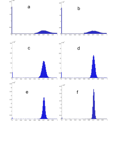
Figure 3: Simulation results for the $(N,[0,1])$-model. The histograms represent observed energies during 100,000 (a,b) and 200,000 iterations (c-f). The system size was 3 sites (a,b), 30 sites (c,d) and 100 sites (e,f). (a),(c) and (e) are boundary sites, (b), (d) and (f) are central sites.

We performed Monte Carlo simulations of the $(N,[0,1])$-model, for various values of $N$. Figure 3 shows histograms of the energies that a site assumes during all the iterations. We started from the empty configuration, but omitted the first 10$\%$ of the observations to avoid recording transient behavior. Further increasing this percentage, or the number of iterations, had no visible influence on the results.

The presented results show that, as the number of sites of the model increases, the energy becomes more and more concentrated around a value close to 0.7. In the next section, we present an argument for this value to be $\sqrt{1/2}$. We further observe that it seems to make a difference where the site is located: at the boundary the variance seems to be larger than in the middle.

6.3 The expected stationary energy per site as $N\to\infty$

From the simulations it appears that for large values of $N$, the energy per site concentrates at a value close to 0.7, for every site. Below we argue, under some assumptions that are consistent with our simulations, that this value should be $\sqrt{1/2}$.

First, we assume that every site has the same expected stationary energy. Moreover, we assume that pairs of sites are asymptotically independent, i.e., $\eta_{x}$ becomes independent of $\eta_{y}$ as $|x-y|\to\infty$. (If the stationary measure is indeed such that the energy of every site is a.s. equal to a constant, then this second assumption is clearly true.) With ${\mathbb{E}}_{\upsilon_{N}}$ denoting expectation with respect to the stationary distribution $\upsilon_{N}$, we say that $(\upsilon_{N})_{N}$ is asymptotically independent if for any $1\leq x_{N},y_{N}\leq N$ with $|x_{N}-y_{N}|\to\infty$, and for any $A,B$ subsets of $\mathbb{R}$ with positive Lebesgue measure, we have

$$\lim_{N\to\infty}\left({\mathbb{E}}_{\upsilon_{N}}({\bf 1}_{\eta_{x_{N}}\in B}|\eta_{y_{N}}\in A)-{\mathbb{E}}_{\upsilon_{N}}({\bf 1}_{\eta_{x_{N}}\in A}\right)=0.$$ (44)

Theorem 6.2.

Suppose that in the $(N,[0,1])$ model, for any sequence $j_{N}\in\{1,\ldots,N\}$,

$$\lim_{N\to\infty}{\mathbb{E}}_{\upsilon_{N}}(\eta_{j_{N}})=\rho,$$ (45)

for some constant $\rho$. Suppose in addition that $(\upsilon_{N})_{N}$ is asymptotically independent. Then we have $\rho=\sqrt{\frac{1}{2}}$.

Proof.

The proof is based on a conservation argument. If we pick a configuration according to $\upsilon_{N}$ and we make an addition $U$, we denote the random amount that leaves the system by $E_{out,N}$. By stationarity, the expectation of $U$ must be the same as the expectation of $E_{out,N}$.

The amount of energy that leaves the system in case of an avalanche, depends on whether or not one of the sites is empty (or behaves as empty). Remember (Proposition 3.2) that when we pick a configuration according to the stationary distribution, then there can be at most one empty or anomalous site. If there is one empty site, then the avalanche reaches one boundary. If there are only full sites, then the avalanche reaches both boundaries, and in case of one anomalous site, both can happen.

However, configurations with no empty site have vanishing probability as $N\to\infty$: we claim that the stationary probability for a configuration to have no empty site, is bounded above by $p_{N}$, with $\lim_{N\to\infty}p_{N}=0$. To see this, we divide the support of the stationary distribution into two sets: $\mathcal{E}$, the set of configurations with one empty site, and $\mathcal{N}$, the set of configurations with no empty site. The only way to reach $\mathcal{N}$ from $\mathcal{E}$, is to make an addition precisely at the empty site. As $X$ is uniformly distributed on $\{1,\ldots,N\}$, this has probability $\frac{1}{N}$, irrespective of the details of the configuration. The only way to reach $\mathcal{E}$ from $\mathcal{N}$, is to cause an avalanche; this certainly happens if an addition of at least $1/2$ is made to a full site. Again, since $X$ is uniformly distributed on $\{1,\ldots,N\}$, and since there is at most one non-full site, this has probability at least $\frac{1}{2}\frac{N-1}{N}$.

Now let $X$ be the (random) addition site at a given time, and denote by $A_{x}$ the event that $X=x$ and that this addition causes the start of an avalanche. Since $E_{out,N}=0$ when no avalanche is started, we can write

$${\mathbb{E}}_{\upsilon_{N}}(E_{out,N})=\sum_{x=1}^{N}{\mathbb{E}}_{\upsilon_{N}}(E_{out,N}|A_{x}){\mathbb{P}}_{\upsilon_{N}}(A_{x}).$$ (46)

We calculate ${\mathbb{P}}_{\upsilon_{N}}(A_{x})$ as follows, writing $U$ for the value of the addition:

$${\mathbb{P}}_{\upsilon_{N}}(A_{x}) = \frac{1}{N}{\mathbb{P}}_{\upsilon_{N}}(\eta_{x}+U\geq 1)=\frac{1}{N}{\mathbb{P}}_{\upsilon_{N}}(U\geq 1-\eta_{x})$$ (47)

$$= \frac{1}{N}\int{\mathbb{P}}_{\upsilon_{N}}(U\geq 1-\eta_{x})d\upsilon_{N}(\eta)=\frac{1}{N}\int\eta_{x}d\upsilon_{N}(\eta)$$

$$= \frac{1}{N}{\mathbb{E}}_{\upsilon_{N}}(\eta_{x}).$$

Let $L_{N}=\lceil\log N\rceil$. Even if the avalanche reaches both boundary sites, the amount of energy that leaves the system can never exceed 2, which implies that

$$\left|\sum_{x=1}^{N}{\mathbb{E}}_{\upsilon_{N}}(E_{out,N}|A_{x})-\sum_{x=2L_{N}}^{N-2L_{N}}{\mathbb{E}}_{\upsilon_{N}}(E_{out,N}|A_{x})\right|\leq 8L_{N}.$$ (48)

It follows from (46), (47) and (48) that

$${\mathbb{E}}_{\upsilon_{N}}(E_{out,N})=\frac{1}{N}\sum_{x=2L_{N}}^{N-2L_{N}}{\mathbb{E}}_{\upsilon_{N}}(E_{out,N}|A_{x}){\mathbb{E}}_{\upsilon_{N}}(\eta_{x})+O(L_{N}/N).$$ (49)

If the avalanche, started at site $x$, reaches the boundary at site 1, then the amount of energy that leaves the system is given by $\frac{1}{2}\eta_{1}+\frac{1}{4}\eta_{2}+\cdots+(\frac{1}{2})^{x}(\eta_{x}+U)$. For all $x\in\{2L_{N},\ldots,N-2L_{N}\}$, this can be written as

$$\frac{1}{2}\eta_{1}+\frac{1}{4}\eta_{2}+\cdots+(\frac{1}{2})^{L_{N}}\eta_{L_{N}}+(\frac{1}{2})^{L_{N}+1}\eta_{L_{N}+1}+\cdots+(\frac{1}{2})^{x}(\eta_{x}+U),$$

where for the last part of this expression, we have the bound

$$(\frac{1}{2})^{L_{N}+1}\eta_{L_{N}+1}+\cdots+(\frac{1}{2})^{x}(\eta_{x}+U)\leq(\frac{1}{2})^{L_{N}}.$$

Since the occurrence of $A_{x}$ depends only on $\eta_{x}$ (and on $X$ and $U$), for $2L_{N}\leq x\leq N-2L_{N}$, by asymptotic independence there is an $\alpha_{N}$, with $\lim_{N\to\infty}\alpha_{N}=0$, such that for all $1\leq i\leq L_{N}$ and $2L_{N}\leq x\leq N-2L_{N}$, we have

$$|{\mathbb{E}}_{\upsilon_{N}}(\eta_{i}|A_{x})-{\mathbb{E}}_{\upsilon_{N}}(\eta_{i})|\leq\alpha_{N},$$

so that

$$\left|{\mathbb{E}}_{\upsilon_{N}}\left(\frac{1}{2}\eta_{1}+\cdots+(\frac{1}{2})^{L_{N}}\eta_{L_{N}}|A_{x}\right)-{\mathbb{E}}_{\upsilon_{N}}\left(\frac{1}{2}\eta_{1}+\cdots+(\frac{1}{2})^{L_{N}}\eta_{L_{N}}\right)\right|\leq\left(\frac{1}{2}+\frac{1}{4}+\cdots\right)\alpha_{N},$$

which is bounded above by $\alpha_{N}$. By symmetry, we have a similar result in the case that the other boundary is reached. In case both boundaries are reached, we simply use that the amount of energy that leaves the system is bounded above by 2.

In view of this, we continue the bound in (49) as follows

$${\mathbb{E}}_{\upsilon_{N}}(E_{out,N}) = \frac{1}{N}\sum_{x=2L_{N}}^{N-2L_{N}}\left({\mathbb{E}}_{\upsilon_{N}}(\frac{1}{2}\eta_{1}+\frac{1}{4}\eta_{2}+\cdots+(\frac{1}{2})^{L_{N}}\eta_{L_{N}}|A_{x})+O((\frac{1}{2})^{L_{N}})\right){\mathbb{E}}_{\upsilon_{N}}(\eta_{x})+$$

$$+O(L_{N}/N)$$

$$= \frac{1}{N}\sum_{x=2L_{N}}^{N-2L_{N}}{\mathbb{E}}_{\upsilon_{N}}(\frac{1}{2}\eta_{1}+\frac{1}{4}\eta_{2}+\cdots+(\frac{1}{2})^{L_{N}}\eta_{L_{N}}){\mathbb{E}}_{\upsilon_{N}}(\eta_{x})+$$

$$+O(\frac{L_{N}}{N})+O((\frac{1}{2})^{L_{N}})+O(\alpha_{N})+O(p_{N}),$$

as $N\to\infty$. Letting $N\to\infty$ and inserting (45) now gives

$$\lim_{N\to\infty}{\mathbb{E}}_{\upsilon_{N}}(E_{out,N})=\rho^{2}.$$

As the expectation of $U$ is $\frac{1}{2}$, we conclude that $\rho=\sqrt{\frac{1}{2}}$. ∎

References

• [1] P. Blanchard, B. Cessac, T. Krüger: A Dynamical System Approach to SOC Models of Zhang’s Type. Journ. of Stat. Phys. 88(1/2), 307-318 (1997)
• [2] D. Dhar: Self-Organized Critical State of Sandpile Automaton Models. Phys. Rev. Lett. 64(14), 1613-1616 (1990)
• [3] O. Diekmann, S.A. van Gils, S.M. Verduyn Lunel and H.-O. Walther: Delay equations; Applied Mathematical Sciences vol. 110. Springer-Verlag, New York, 1995
• [4] R.M. Dudley: Real Analysis and Probability. Wadsworth & Brooks/Cole, California, 1989
• [5] W. Feller: An Introduction to Probability Theory and its Applications, vol. II. John Wiley and Sons, Inc., USA, 1966
• [6] I.M. Janosi: Effect of anisotropy on the self-organized critical state. Phys. Rev. A 42(2), 769-774 (1989)
• [7] R. Meester, F. Redig and D. Znamenski: The abelian sandpile model; a mathematical introduction. Markov Proc. Rel. Fields 7, 509-523 (2001)
• [8] R. Pastor-Satorras and A. Vespignani: Anomalous scaling in het Zhang model. Eur. Phys. J. B 18, 197-200 (2000)
• [9] E.V. Ivashkevich and V.B. Priezzhev: Introduction to the sandpile model. Physica A 254, 97–116 (1998)
• [10] C. Maes, F. Redig, E. Saada and A. van Moffaert: On the thermodynamic limit for a one-dimensional sandpile process. Markov Proc. and Rel. Fields 6(1), 1-21 (2000)
• [11] H. Thorisson: Coupling, Stationarity, and Regeneration. Springer Verlag, New York, 2000
• [12] D.L. Turcotte: Self-organized criticality. Reports on progress in physics 62 (10), 1377-1429 (1999)
• [13] Y.-C. Zhang: Scaling theory of Self-Organized Criticality. Phys. Rev. Lett. 63(5), 470-473 (1989)