Abstract

We present an algorithm for characterising the generalised Dirichlet to Neumann map for moving initial-boundary value problems. This algorithm is derived by combining the so-called global relation, which couples the initial and boundary values of the problem, with a new method for inverting certain one-dimensional integrals. This new method is based on the spectral analysis of an associated ODE and on the use of the d-bar formalism. As an illustration, the Neumann boundary value for the linearised Schrödinger equation is determined in terms of the Dirichlet boundary value and of the initial condition.

1 Introduction

We present a methodology for characterising the generalised Dirichlet to Neumann map for linear evolution PDEs posed on domains whose boundary varies with time. Consider, as an example, the following domain in the $(x,t)$ plane, see figure 1:

$${\bf D}:\quad 0<t<T,\quad l(t)<x<\infty,$$ (1.1)

where $T$ is a positive constant and $l(t)$ is a given monotonic, twice differentiable function. For economy of presentation we assume that $l(t)$ satifies the following:

$$l(t)\in{\bf C}^{2}[0,T],\quad l^{\prime\prime}(t)>0,\quad l(0)=0.$$

Let the scalar complex-valued function $q(x,t)$ satisfy the boundary value problem

$$iq_{t}+q_{xx}=0,\quad(x,t)\in{\bf D},$$

$$q(x,0)=q_{0}(x),\;\;0<x<\infty;\quad q(l(t),t)=f_{0}(t),\;\;0<t<T.$$ (1.2)

We assume that the initial condition $q_{0}(x)$ is a sufficiently smooth function, decaying as $x\to~{}\infty$, that the boundary condition $f_{0}(t)$ is sufficiently smooth, and that these two functions are compatible at the origin, $q_{0}(0)=f_{0}(0)$.

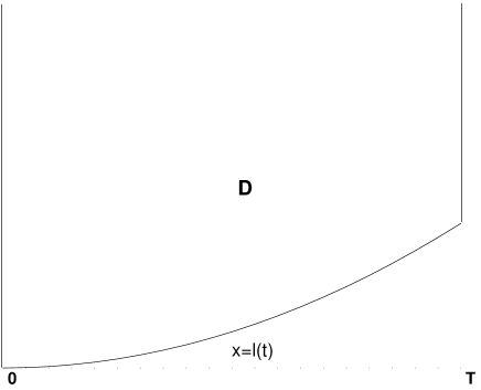
Figure 1: The domain ${\bf D}$ in the $(x,t)$ plane

There exist several different integral representations for the solution of initial-boundary value problems such as those defined by (1.2). These include the representation constructed by using the classical Fourier transform in the $x$ variable, as well as the novel representations presented in [6, 7]. However, these representations are not effective, because they involve unknown boundary values. For example, for the initial-boundary value problem (1.2) these representations involve the unknown function $q_{x}(l(t),t)$.

Thus, the key issue is the characterisation of the generalised Dirichlet to Neumann map, namely the characterisation of the unknown boundary values in terms of the given initial and boundary conditions. For the initial-boundary value problem (1.2) this means computing $q_{x}(l(t),t)$ in terms of $\{q_{0}(x),f_{0}(t)\}$.

Here we present an algorithm for constructing the generalised Dirichlet to Neumann map. For the initial boundary value problem (1.2) this algorithm yields the unknown function $q_{x}(l(t),t)=f_{1}(t)$ through the solution of the Volterra integral equation

$$f_{1}(t)=\frac{2}{3\pi}\int_{0}^{t}J(s,t)f_{1}(s)ds+$$ (1.3)

$$+\frac{2}{3\sqrt{\pi}}{\rm e}^{-i\pi/4}\left[\int_{0}^{t}\frac{{\rm e}^{i\frac{(l(t)-l(s))^{2}}{4(t-s)}}}{\sqrt{t-s}}f_{0}^{\prime}(s)ds+\frac{1}{\sqrt{t}}\int_{0}^{\infty}{\rm e}^{\frac{i(l(t)-x)^{2}}{4t}}q_{0}^{\prime}(x)dx\right],$$

for $0<t<T$, where the kernel $J(s,t)$ is defined by

$$J(s,t)=\frac{l(s)-l(t)}{2(s-t)}\left\{\int_{l^{\prime}(s)/2}^{\infty}{\rm e}^{ik^{2}(s-t)-ik(l(s)-l(t))}dk-i\,G(s,t)\int_{0}^{\infty}{\rm e}^{-ik^{2}(s-t)-k(s-t)\left[l^{\prime}(s)-\frac{l(s)-l(t)}{s-t}\right]}dk\right\},$$ (1.4)

and

$$G(s,t)={\rm e}^{i\frac{l^{\prime}(s)^{2}}{4}(s-t)-i\frac{l^{\prime}(s)}{2}(l(s)-l(t))}.$$ (1.5)

We note the both integrals on the right hand side of equation (1.4) are well defined. In particular, the second integral involves an exponential which decays as $k\to\infty$. Indeed, the real part of the exponent is

$$-k(s-t)\left(l^{\prime}(s)-\frac{l(t)-l(s)}{t-s}\right)=-k(s-t)(l^{\prime}(s)-l^{\prime}(\sigma)),\quad s\leq\sigma\leq t.$$

Recalling that $l^{\prime\prime}(t)>0$, it follows that $l^{\prime}(s)-l^{\prime}(\sigma)\leq 0$, and since $k\geq 0$ and $s-t\leq 0$, the real part of the exponent is negative.

The algorithm involves three steps:

1. Assuming that the solution exists, derive the so-called global relation, namely the relation that couples the initial condition with all boundary values. This step is elementary and it involves only writing the given PDE in a proper divergence form, and applying Green’s theorem. For example, equation (1.2) can be rewritten in the form

$$\left[{\rm e}^{-ikx+ik^{2}t}q(x,t)\right]_{t}-\left[{\rm e}^{-ikx+ik^{2}t}(iq_{x}(x,t)-kq(x,t)\right]_{x}=0,\quad k\in\mathbb{C}.$$ (1.6)

Then an application of Green’s theorem in the domain ${\bf D}$ yields

$$i\int_{0}^{T}{\rm e}^{ik^{2}s-ikl(s)}q_{x}(l(s),s)ds=\int_{0}^{T}{\rm e}^{ik^{2}s-ikl(s)}(k-l^{\prime}(s))f_{0}(s)ds$$

$$+\hat{q}_{0}(k)-{\rm e}^{ik^{2}T}\int_{l(T)}^{\infty}{\rm e}^{-ikx}q(x,T)dx,\quad{\rm Im}(k)\leq 0.$$ (1.7)

2. Consider the integral involving the unknown boundary values and derive a general formula for the inversion of this type of integrals. This step involves the spectral analysis of an appropriate ODE. For example, for the initial boundary value problem (1.2), this ODE is

$$\mu_{t}(t,k)+(ik^{2}-ikl^{\prime}(t))\mu(t,k)=kf(t),\quad 0<t<T,\;\;k\in\mathbb{C}.$$ (1.8)

Using this ODE it is shown in Section 2 that if $F(k)$ is defined in terms of $f(s)$ by the integral

$$F(k)=\int_{0}^{T}{\rm e}^{ik^{2}s-ikl(s)}f(s)ds,\quad k\in\mathbb{C},$$ (1.9)

then $f(t)$ can be obtained in terms of $F(k)$ through the solution of the following Volterra integral equation

$$f(t)=\frac{2}{3\pi}\int_{\partial\Omega_{2}^{-}(t)}{\rm e}^{-ik^{2}t+ikl(t)}F(k)kdk+\frac{2}{3\pi}\int_{0}^{t}J(s,t)f(s)ds,\quad 0<t<T,$$ (1.10)

where $J(s,t)$ is defined by equation (1.4) and $\partial\Omega_{2}^{-}(t)$ is given by

$$\partial\Omega_{2}^{-}(t)=\{k\in\mathbb{R}:\;k\leq l^{\prime}(t)/2\}\cup\{k=k_{R}+ik_{I}:\;k_{R}=l^{\prime}(t)/2,\;k_{I}\leq 0\}$$ (1.11)

with the orientation shown in Figure 2.

Figure 2: The curve $\partial\Omega_{2}^{-}(t)$ in the $k$ plane

3. Use the global relation (1.7) and the inversion formula (1.10) to derive a Volterra integral equation for the unknown boundary values. The global relation (1.7) is of the form (1.9) where $f(t)$ and $F(k)$ are replaced respectively by $if_{1}(t)$ and by

$$\hat{q}_{0}(k)-{\rm e}^{ik^{2}T}\int_{l(T)}^{\infty}{\rm e}^{-ikx}q(x,T)dx+\int_{0}^{T}{\rm e}^{ik^{2}s-ikl(s)}(k-l^{\prime}(s))f_{0}(s)ds.$$ (1.12)

Furthermore, the global relation is valid for $Im(k)\leq 0$, therefore it is valid for $k\in\,\partial\Omega_{2}^{-}(t)$. It is shown in Section 3 that equation (1.3) follows from equation (1.10) by replacing in equation (1.9) $f(s)$ and $F(k)$ by $if_{1}$ and by the expression in (1.12).

It turns out that the second term in (1.12) yields a zero contribution, which is consistent with the evolutionary nature of equation (1.2) ($q(x,t)$ cannot depend on the future time $T$).

Although the generalised Dirichlet to Neumann map is obtained under the assumption of the existence of a unique solution, this map can be justified a posteriori without this assumption, see Theorem 1.1 of [7].

2 The spectral analysis of ordinary differential equations and the inversion of complex integrals

Proposition 2.1

Let $F(k)$ be defined in terms of $f(t)$ by equation (1.9), where $f(t)$ is a sufficiently smooth function. Then $f(t)$ satisfies the Volterra integral equation (1.10).

Proof: (a) We first treat the ODE (1.8) as an equation which defines $\mu(t,k)$ in terms of $f(t)$ and we seek a solution which is bounded for all values of the complex parameter $k$.

By integrating with respect to $t$ from either $0$ or $T$ we find the following two particular solutions of (1.8):

$$\mu_{1}(t,k) = \int_{0}^{t}{\rm e}^{i(k^{2}(s-t)-k(l(s)-l(t))}kf(s)ds,$$ (2.1)

$$\mu_{2}(t,k) = -\int_{t}^{T}{\rm e}^{i(k^{2}(s-t)-k(l(s)-l(t))}kf(s)ds.$$ (2.2)

The functions $\mu_{1}$ and $\mu_{2}$ are entire functions of $k$, which are bounded, respectively, in the domains $\Omega_{1}$ and $\Omega_{2}$ defined by

$$\Omega_{1}(t) = \{k\in\mathbb{C}:\;k_{I}\geq 0,\;k_{R}\leq\frac{l^{\prime}(0)}{2}\}\cup\{k\in\mathbb{C}:\;k_{I}<0,\;k_{R}\geq\frac{l^{\prime}(t)}{2},\;0<t<T\}.$$

$$\Omega_{2}(t) = \{k\in\mathbb{C}:\;k_{I}\geq 0,\;k_{R}>\frac{l^{\prime}(T)}{2}\}\cup\{k\in\mathbb{C}:\;k_{I}\leq 0,\;k_{R}\leq\frac{l^{\prime}(t)}{2},\;0<t<T\}.$$

The domains $\Omega_{1}(t)$ and $\Omega_{2}(t)$, which are depicted in figure 3, are determined by the real part of the exponent of the exponential term appearing in equations (2.1),(2.2), which equals

$${\rm e}^{-(s-t)k_{I}(2k_{R}-\frac{l(s)-l(t)}{s-t})}={\rm e}^{-(s-t)k_{I}(2k_{R}-l^{\prime}(\tau))},$$

where $\tau$ is in the interval bounded by $s$ and $t$.

For $\mu_{1}$, $s-t\leq 0$, thus $\mu_{1}$ is bounded if and only if

$$k_{I}(2k_{R}-l^{\prime}(\tau))\leq 0,$$

i.e.

$$\{k_{I}\geq 0,\;k_{R}\leq\frac{l^{\prime}(\tau)}{2}\}\;{\rm or}\;\{k_{I}\leq 0,\;k_{R}\geq\frac{l^{\prime}(\tau)}{2}\},$$

for every $\tau$ in the interval $0<s<\tau<t$. Taking into account that $l^{\prime}(t)$ is an increasing function, the above inequalities yield the definition of $\Omega_{1}$. Similarly for $\mu_{2}$ and $\Omega_{2}(t)$.

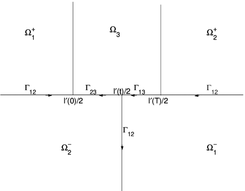
Figure 3: The domains $\Omega_{1}$, $\Omega_{2}$ and $\Omega_{3}$ in the $k$-plane and the contours $\Gamma_{12}$,$\Gamma_{13}$ and $\Gamma_{23}$

A solution of the ODE (1.8) which is bounded in the domain

$$\Omega_{3}=\{k\in\mathbb{C}:\;k_{I}\geq 0,\;\frac{l^{\prime}(0)}{2}\leq k_{R}\leq\frac{l^{\prime}(T)}{2}\},$$ (2.5)

is given by

$$\mu_{3}(t,k,\bar{k})=\int_{S(k_{R})}^{t}{\rm e}^{i(k^{2}(s-t)-k(l(s)-l(t))}kf(s)ds,$$ (2.6)

where the function $S(k_{R})$ is defined on the real interval $[\frac{l^{\prime}(0)}{2},\frac{l^{\prime}(T)}{2}]$ by

$$S(k_{R}):[\frac{l^{\prime}(0)}{2},\frac{l^{\prime}(T)}{2}]\to[0,T],\quad S(k_{R})=s\Longleftrightarrow k_{R}=\frac{l^{\prime}(s)}{2}.$$ (2.7)

In order to prove that the function $\mu_{3}$ is bounded in $\Omega_{3}$, we distinguish two cases:

• $0\leq S(k_{R})<t$

  In this case, $s-t\leq 0$ and since $k_{I}\geq 0$, we need to prove that $k_{R}\leq l^{\prime}(\tau)/2$, which follows from the fact that $l^{\prime}(\tau)/2>l^{\prime}(s)/2\geq k_{R}$.

• $t<S(k_{R})\leq T$

  In this case, $s-t\geq 0$ and since $k_{I}\geq 0$, we need to prove that $k_{R}\geq l^{\prime}(\tau)/2$, which follows from the fact that $l^{\prime}(\tau)/2<l^{\prime}(s)/2\leq k_{R}$.

We emphasise that the function $\mu_{3}(t,k,\bar{k})$, in contrast with the functions $\mu_{1}(t,k)$ and $\mu_{2}(t,k)$, involves $k_{R}$, hence this function dependes on both $k$ and $\bar{k}$.

Integration by parts of the equations defining the $\mu_{j}$’s implies the following asymptotic behaviour

$$\mu_{j}=O\left(\frac{1}{k}\right),\quad k\in\;\Omega_{j},\quad k\to\infty,\quad j=1,2,3.$$ (2.8)

Equations (2.1), (2.2) and (2.6) define a function $\mu(t,k,\bar{k})$ in terms of $f(t)$.

(b) Using the fact that the function $\mu(t,k,\bar{k})$ is bounded in the entire complex $k$ plane, including infinity (see equation (2.8)), it is possible to find an alternative representation for this function using the Pompeiu ( also known as Cauchy-Green, or d-bar) formula [1],

$$\mu(t,k,\bar{k})=\frac{1}{2\pi i}\int_{\gamma(t)}\frac{\rm``jumps^{\prime\prime}}{\lambda-k}d\lambda+\frac{1}{2\pi i}\int\int_{\Omega(t)}\frac{\partial\mu(t,\lambda,\bar{\lambda})}{\partial\bar{\lambda}}\frac{d\lambda\wedge d\bar{\lambda}}{\lambda-k},\quad 0<t<T,\,k\in\mathbb{C},$$ (2.9)

where $d\lambda\wedge d\bar{\lambda}=-2id\lambda_{R}d\lambda_{I}$, $\gamma(t)$ denotes the contour along which the function $\mu$ has a “jump” discontinuity and $\Omega(t)$ is the domain where $\partial\mu/\partial\bar{k}\neq 0$. Before computing the relevant jumps, we note that $\mu_{3}$ coincide with $\mu_{1}$ on the half-line $\{k_{I}>0,\;k_{R}=l^{\prime}(0)/2\}$ and with $\mu_{2}$ on the half-line $\{k_{I}>0,\;k_{R}=l^{\prime}(T)/2\}$. This is consequence of the definition of $S(k_{R})$, which implies that $S(l^{\prime}(s)/2)=s$ for all $0\leq s\leq T$. Thus, the relevant jumps are given by the expressions

$$\mu_{1}-\mu_{2} = \int_{0}^{T}A(k,s,t,)ds,\quad k\in\,\Gamma_{12},$$

$$\mu_{1}-\mu_{3} = \int_{0}^{S(k_{R})}A(k,s,t,)ds,\quad k\in\,\Gamma_{13},$$

$$\mu_{2}-\mu_{3} = \int_{T}^{S(k_{R})}A(k,s,t,)ds,\quad k\in\,\Gamma_{23},$$ (2.10)

where we use the following notation (see figure 3):

$$A(k,s,t) = {\rm e}^{ik^{2}(s-t)-ik(l(s)-l(t))}kf(s),$$ (2.11)

$$\Gamma_{12}(t) = \{k_{I}=0,\;k_{R}\in\,(-\infty,\frac{l^{\prime}(0)}{2})\}\cup\{k_{R}=\frac{l^{\prime}(t)}{2},\;k_{I}\in\,(0,-\infty)\}\cup$$

$$\cup\{k_{I}=0,\;k_{R}\in(\infty,l^{\prime}(T)/2)\},$$

$$\Gamma_{13}(t) = \{k_{I}=0,\;k_{R}\in\,(\frac{l^{\prime}(T)}{2},\frac{l^{\prime}(t)}{2})\},$$ (2.12)

$$\Gamma_{23}(t) = \{k_{I}=0,\;k_{R}\in\,(\frac{l^{\prime}(t)}{2},\frac{l^{\prime}(0)}{2})\}.$$

The direction of integration is depicted in figure 3, and it is also indicated in equations (2.12); for example, $k_{R}\in(-\infty,l^{\prime}(0)/2)$ indicates that the integration is from $-\infty$ to   $l^{\prime}(0)/2$.

Equation (2.6) implies

$$\frac{\partial\mu_{3}(t,k,\bar{k})}{\partial\bar{k}}=-\frac{\partial S(k_{R})}{\partial\bar{k}}k\{{\rm e}^{ik^{2}(s-t)-k(l(s)-l(t))}f(s)\}_{s=S(k_{R})}=-\frac{\partial S(k_{R})}{\partial\bar{k}}A(k,S(k_{R}),t).$$ (2.13)

Hence, using equations (2.10) and (2.13) in equation (2.9), we find the following alternative representation of $\mu$:

$$\mu(t,k,\bar{k})=\frac{1}{2\pi i}\int_{\Gamma_{12}}\left(\int_{0}^{T}A(\lambda,s,t)ds\right)\frac{d\lambda}{\lambda-k}+\frac{1}{2\pi i}\int_{\Gamma_{13}}\left(\int_{0}^{S(k_{R})}A(\lambda,s,t)ds\right)\frac{d\lambda}{\lambda-k}$$

$$+\frac{1}{2\pi i}\int_{\Gamma_{23}}\left(\int_{T}^{S(k_{R})}A(\lambda,s,t)ds\right)\frac{d\lambda}{\lambda-k}-\frac{1}{2\pi i}\int\int_{\Omega_{3}}\frac{\partial S(\lambda_{R})}{\partial\bar{\lambda}}A(\lambda,S(\lambda_{R}),t)\frac{d\lambda\wedge d\bar{\lambda}}{\lambda-k}.$$ (2.14)

(c) The representation of the function $\mu(t,k,\bar{k})$ defined by equations (2.1), (2.2), (2.6) involves $f(t)$, while the represnetation defined by equation (2.14) involves various integrals of $A(k,s,t)$. Thus there exists a relation between $f(t)$ and these integrals of $A$. The simplest way to obtain this relation is to consider the large $k$ asymptotic behaviour of $\mu(t,k,\bar{k})$. Equation (2.14) implies

$$\mu(t,k,\bar{k})=\frac{\mu_{0}(t)}{k}+O\left(\frac{1}{k}\right),\quad\mu_{0}=\lim_{k\to\infty}(k\mu).$$

Substituting this expression in the ODE (1.8) we find $\mu_{0}=f(t)$, thus

$$f(t)=\frac{1}{2\pi}\left\{-\int_{\Gamma_{12}}\left(\int_{0}^{T}A(k,s,t)ds\right)dk-\int_{\Gamma_{13}}\left(\int_{0}^{S(k_{R})}A(k,s,t)ds\right)dk\right.$$

$$-\left.\int_{\Gamma_{23}}\left(\int_{T}^{S(k_{R})}A(k,s,t)ds\right)dk+\int\int_{\Omega_{3}}\frac{\partial S(k_{R})}{\partial\bar{k}}A(k,S(k_{R}),t)dk\wedge d\bar{k}\right\}.$$ (2.15)

Equation (2.15) was first derived in [7] (see equation (3.2) of [7]).

(d) We will now show that equation (2.15) can be transformed into a Volterra integral equation. For this purpose, we split the domain $\Omega_{3}$ in the form $\Omega_{3}=\Omega_{3}^{(1)}(t)\cup\Omega_{3}^{(2)}(t)$ where

$$\Omega_{3}^{(1)}(t)=\{k\in\Omega_{3}:l^{\prime}(0)/2<k_{R}<l^{\prime}(t)/2\},\quad\Omega_{3}^{(2)}(t)=\{k\in\Omega_{3}:l^{\prime}(t)/2<k_{R}<l^{\prime}(T)/2\}.$$ (2.16)

In the domain $\Omega_{3}^{(2)}(t)$ we use the complex form of Green’s theorem, which states that

$$-\int\int_{\Omega_{3}^{(2)}(t)}\frac{\partial\mu_{3}(k,\bar{k})}{\partial\bar{k}}dk\wedge d\bar{k}=\int_{\partial\Omega_{3}^{(2)}(t)}\mu_{3}(k,\bar{k})dk,$$ (2.17)

where the boundary $\partial\Omega_{3}^{(2)}(t)$ of $\Omega_{3}^{(2)}(t)$ has counterclockwise orientation. Recalling that $S(k_{R})=t$ when $2k_{R}=l^{\prime}(t)$, it follows that the contribution of the half line $\{k_{R}=l^{\prime}(t)/2,k_{I}>0\}$ to the right hand side of equation (2.17) vanishes, hence

$$\int\int_{\Omega_{3}^{(2)}(t)}\frac{\partial S(k_{R})}{\partial\bar{k}}A(k,S(k_{R}),t)dk\wedge d\bar{k}=-\int\int_{\Omega_{3}^{(2)}(t)}\frac{\partial\mu_{3}(k,\bar{k})}{\partial\bar{k}}dk\wedge d\bar{k}=$$

$$=\int_{l^{\prime}(t)/2}^{l^{\prime}(T)/2}\int_{S(k_{R})}^{t}A(k,s,t)dsdk+\int_{l(T)}\int_{T}^{t}A(k,s,t)dsdk,$$ (2.18)

where the half line $l(T)$ is defined by

$$l(T)=\{k:k_{R}=l^{\prime}(T)/2,\;0\leq k_{I}<\infty\}.$$ (2.19)

The integrands of the line integrals appearing on the right hand side of equation (2.15) are shown in figure 4, while the integrands of the line integrals appearing on the right hand side of equation (2.18) are shown in figure 5.

Figure 4: The integrands in equation (2.15)

Figure 5: The integrands in equation (2.18)

Adding the integrands in the respective line integrals, we find the contributions depicted in figure (6).

Figure 6: The integrands in the expression obtained by adding (2.15) and (2.18) together. The double lines indicate that the contribution is split into two integrals.

The above analysis, together with the identity

$$\frac{\partial S(k_{R})}{\partial\bar{k}}=\frac{dS(k_{R})}{2dk_{R}},\quad dk\wedge d\bar{k}=-2idk_{R}dk_{I}.$$

implies that equation (2.15) can be rewritten in the following form

$$2\pi f(t) = \int_{\partial\Omega_{2}^{-}(t)}\left(\int_{0}^{T}A(k,s,t)ds\right)\,dk+\int_{\partial\Omega_{2}^{+}(t)}\left(\int_{t}^{T}A(k,s,t)ds\right)dk$$ (2.20)

$$+ \int_{l^{\prime}(0)/2}^{l^{\prime}(t)/2}\left(\int_{0}^{S(k_{R})}A(k,s,t)ds\right)dk+\left\{\int_{l^{\prime}(t)/2}^{\infty}\left(\int_{0}^{t}A(k,s,t)ds\right)dk\right.$$

$$- i\left.\int_{0}^{\infty}\left(\int_{l^{\prime}(0)/2}^{l^{\prime}(t)/2}\left(\frac{dS(k_{R})}{dk_{R}}\right)A(k,S(k_{R}),t)dk_{R}\right)dk_{I},\right\}.$$

As a consequence of splitting the integrals originally appearing together on the right hand side of equation (2.14), the resulting individual integrals in equation (2.20) have a singularity as $k\to\infty$. Hence the last two integrals on the right hand side of equation (2.20) must be considered together (this is indicated by the curly brackets around these terms).

The first term on the right hand side of this expression can be computed in terms of the given data $F(k)$, defined in (1.9), hence this term is known.

The second term equals $(\pi/2)f(t)$. Indeed, the integrand in this term is bounded and analytic in $\Omega_{2}^{+}(t)$, and it behaves like $if(t)/k$ as $k\to\infty$. Thus this term equals

$$if(t)\int_{\pi/2}^{0}id\theta=\frac{\pi}{2}f(t).$$

The third integral in (2.20) can be written in a “Volterra form” by exchanging the order of integration. Indeed, recalling the definition of $S(k_{R})$ and changing variable to $\sigma=S(k_{R})$ so that $k(=k_{R})=l^{\prime}(\sigma)/2$, we find that this integral is equal to

$$\int_{l^{\prime}(0)/2}^{l^{\prime}(t)/2}\left(\int_{0}^{S(k_{R})}A(k,s,t)ds\right)dk=\int_{0}^{t}\left(\int_{l^{\prime}(s)/2}^{l^{\prime}(t)/2}A(k,s,t)dk\right)ds$$

In the double integral we change the variable $k_{R}$ to $s=S(k_{R})$ and rename $k_{I}$ as $k$. This yields

$$\int_{0}^{\infty}\int_{l^{\prime}(0)/2}^{l^{\prime}(t)/2}\frac{dS(k_{R})}{dk_{R}}A(k,S(k_{R}),t)dk_{R}dk_{I}=\int_{0}^{\infty}\left(\int_{0}^{t}A(\frac{l^{\prime}(s)}{2}+ik,s,t)ds\right)dk.$$

Hence equation (2.20) yields

$$\frac{3\pi}{2}f(t)=\int_{\partial\Omega_{2}^{-}(t)}\left(\int_{0}^{T}A(k,s,t)ds\right)dk+\int_{0}^{t}\left(\int_{l^{\prime}(s)/2}^{l^{\prime}(t)/2}A(k,s,t)dk\right)ds+$$ (2.21)

$$\left\{\int_{l^{\prime}(t)/2}^{\infty}\left(\int_{0}^{t}A(k,s,t)ds\right)dk-i\int_{0}^{\infty}\left(\int_{0}^{t}A(\frac{l^{\prime}(s)}{2}+ik,s,t)ds\right)dk\right\}.$$

Setting

$$A(k,s,t)=E(k,s,t)kf(s),\quad E(k,s,t)={\rm e}^{ik^{2}(s-t)-ik(l(s)-l(t))},$$ (2.22)

and using

$$E(\frac{l^{\prime}(s)}{2}+ik,s,t)=E(ik,s,t){\rm e}^{-k(s-t)l^{\prime}(s)}G(s,t),$$

where $G(s,t)$ is given by (1.5), equation (2.21) becomes

$$\frac{3\pi}{2}f(t)=\int_{\partial\Omega_{2}^{-}(t)}\left(\int_{0}^{T}A(k,s,t)ds\right)dk+\int_{0}^{t}\left(\int_{l^{\prime}(s)/2}^{l^{\prime}(t)/2}E(k,s,t)kdk\right)f(s)ds+$$ (2.23)

$$\left\{\int_{l^{\prime}(t)/2}^{\infty}k\left(\int_{0}^{t}E(k,s,t)f(s)ds\right)dk-i\int_{0}^{\infty}\left(\int_{0}^{t}E(ik,s,t)(k-i\frac{l^{\prime}(s)}{2})G(s,t){\rm e}^{-k(s-t)l^{\prime}(s)}f(s)ds\right)dk\right\}.$$

In what follows we will rewrite the terms in the above bracket in a Volterra form. In this regard we note that this bracket is well defined. Indeed, integration by parts of the inner integrals yields

$$\int_{l^{\prime}(t)/2}^{\infty}\left[\frac{f(t)}{ik}+O\left(\frac{1}{k^{2}}\right)\right]dk\\ -i\int_{0}^{\infty}\left[-\frac{f(t)}{k}+O\left(\frac{1}{k^{2}}\right)\right]dk,$$

which shows that the contribution of the singular term $1/k$ at infinity cancels out.

We start by rewriting the bracket as

$$\int_{0}^{t}\left[J_{1}(s,t)+G(s,t)J_{2}(s,t)-\frac{i}{2}G(s,t)l^{\prime}(s)\tilde{J}_{2}(s,t)\right]f(s)ds$$ (2.24)

where

$$J_{1}(s,t) = \lim_{\varepsilon\to 0^{+}}\int_{l^{\prime}(t)/2}^{\infty}{\rm e}^{ik^{2}(s-t+i\varepsilon)-ik(l(s)-l(t))}kdk,$$

$$J_{2}(s,t) = \lim_{\varepsilon\to 0^{+}}\int_{0}^{\infty}{\rm e}^{-ik^{2}(s-t+i\varepsilon)+k(l(s)-l(t))-k(s-t)l^{\prime}(s)}kdk,$$

$$\tilde{J}_{2}(s,t) = \int_{0}^{\infty}E(ik,s,t){\rm e}^{-k(s-t)l^{\prime}(s)}dk.$$ (2.25)

The kernel in the expression (2.24) equals

$$\frac{H(s,t)}{2i(s-t)}+\frac{l(s)-l(t)}{2(s-t)}\left[\tilde{J}_{1}(s,t)-iG(s,t)\tilde{J}_{2}(s,t)\right]$$ (2.26)

where $G(s,t)$ is given by (1.5) and

$$H(s,t)=G(s,t)-{\rm e}^{i\frac{l^{\prime}(t)^{2}}{4}(s-t)-i\frac{l^{\prime}(t)}{2}(l(s)-l(t))},\quad\tilde{J}_{1}(s,t)=\int_{l^{\prime}(t)/2}^{\infty}E(k,s,t)dk.$$ (2.27)

Indeed, integrating by parts the expressions for $J_{1}$ and $J_{2}$ we find

$$J_{1}(s,t) = -\frac{{\rm e}^{i\frac{l^{\prime}(t)^{2}}{4}(s-t)-i\frac{l^{\prime}(t)}{2}(l(s)-l(t))}}{2i(s-t+i0)}+\frac{l(s)-l(t)}{2(s-t)}\int_{l^{\prime}(t)/2}^{\infty}E(k,s,t)dk,$$ (2.28)

$$J_{2}(s,t) = \frac{1}{2i(s-t+i0)}+\left[\frac{l(s)-l(t)}{2i(s-t)}-\frac{l^{\prime}(s)}{2i}\right]\tilde{J}_{2}(s,t).$$ (2.29)

Substituting the above expressions in (2.24) we find that the kernel equals the expression in (2.26).

Using integration by parts of the second term on the right hand side of (2.23), we find

$$\int_{l^{\prime}(s)/2}^{l^{\prime}(t)/2}E(k,s,t)kdk=-\frac{H(s,t)}{2i(s-t)}+\frac{l(s)-l(t)}{2(s-t)}\int_{l^{\prime}(s)/2}^{l^{\prime}(t)/2}E(k,s,t)dk.$$ (2.30)

Adding the expressions in (2.26) and (2.30) we find that the equation (2.23) can be written in the form

$$\frac{3\pi}{2}f(t)=\int_{\partial\Omega_{2}^{-}(t)}\left(\int_{0}^{T}A(k,s,t)ds\right)dk+\int_{0}^{t}J(s,t)f(s)ds,$$

where $J(s,t)$ is the kernel given by (1.4).

Remark 2.1

The direct evaluation of the first integral appearing in expression (1.4), by completing the square in the exponent, yields

$$\int_{l^{\prime}(s)/2}^{\infty}E(k,s,t)dk={\rm e}^{i\frac{(l(t)-l(s))^{2}}{4(t-s)}}\int_{l^{\prime}(s)/2}^{\infty}{\rm e}^{-i(t-s)[k-\frac{l(s)-l(t)}{2(s-t)}]^{2}}dk$$

Setting $\lambda=[k-\frac{l(s)-l(t)}{2(s-t)}]\sqrt{t-s}$, and $\lambda_{0}(s,t)=\sqrt{t-s}\left[l^{\prime}(s)/2-\frac{l(s)-l(t)}{2(s-t)}\right]$, this can be written as

$$\int_{l^{\prime}(s)/2}^{\infty}E(k,s,t)dk=\frac{{\rm e}^{i\frac{(l(t)-l(t))^{2}}{4(t-s)}}}{\sqrt{t-s}}\int_{\lambda_{0}(s,t)}^{\infty}{\rm e}^{-i\lambda^{2}}d\lambda.$$ (2.31)

The integral on the right hand side of equation (2.31) can be expressed in terms of the Gamma function, and of the imaginary error function Erfi$(z)$. Indeed,

$$\int_{\lambda_{0}(s,t)}^{\infty}{\rm e}^{-i\lambda^{2}}d\lambda=\int_{\lambda_{0}(s,t)}^{0}{\rm e}^{-i\lambda^{2}}d\lambda+\int_{0}^{\infty}{\rm e}^{-i\lambda^{2}}d\lambda=$$

$$=\frac{i+1}{2}\sqrt{\frac{\pi}{2}}{\rm Erfi}({\rm e}^{3\pi i/4}\lambda_{0}(s,t))+\frac{\sqrt{\pi}}{2}{\rm e}^{-i\pi/4}.$$

3 The Dirichlet to Neumann map for the linear Schrödinger equation

Proposition 3.1

Let the complex-valued scalar function $q(x,t)$ satusfy the following initial-boundary value problem:

$$\begin{array}[]{lll}iq_{t}+q_{xx}=0,&l^{\prime}(t)<x<\infty,&0<t<T,\\ q(x,0)=q_{0}(x),&&l^{\prime}(t)<x<\infty,\\ q(l(t),t)=f_{0}(t),&&0<t<T,\\ q_{0}(0)=f_{0}(0)&&\end{array}$$ (3.1)

where $l(t)\in{\bf C}^{2}[0,T],\quad l^{\prime\prime}(t)>0,\quad l(0)=0.$ The Dirichlet to Neumann map for this problem is characterised by the linear Volterra integral equation (1.3).

Proof In order to obtain the linear integral equation satisfied by $f_{1}(t)=q_{x}(l(t),t)$ we must replace in equation (1.10) the function $f(t)$ by $if_{1}(t)$, and the function $F(k)$ by the expression in (1.12). Multiplying the latter expression by $k$ we find three terms.

The first term in (1.12), multiplied by $k$, equals

$$k\int_{0}^{\infty}{\rm e}^{-ikx}q_{0}(x)dx=-iq_{0}(0)-i\int_{0}^{\infty}{\rm e}^{-ikx}q_{0}^{\prime}(x)dx.$$ (3.2)

The second term multiplied by $k{\rm e}^{-ik^{2}t+ikl(t)}$ is

$$k{\rm e}^{ik^{2}(T-t)-ik(l(T)-l(t))}\int_{l(T)}^{\infty}{\rm e}^{-ik(x-l(T))}q(x,T)dx.$$ (3.3)

The exponential multiplying the above integral is bounded in the domain $\Omega_{2}^{-}(t)$, while the integral in (3.3) is bounded and analytic for Im$(k)\leq 0$ and is of order $O\left(\frac{1}{k}\right)$ as $k\to\infty$. Thus, the application of Jordan’s lemma (after a suitable change of variables) implies that the integral of (3.3) along $\partial\Omega_{2}^{-}(t)$ vanishes.

The third term in (1.12), multiplied by $k$, equals

$$\int_{0}^{T}{\rm e}^{ik^{2}s-ikl(s)}(k^{2}-kl^{\prime}(s))f_{0}(s)ds=-i{\rm e}^{ik^{2}T-ikl(T)}f_{0}(T)+if_{0}(0)+i\int_{0}^{T}{\rm e}^{ik^{2}s-ikl(s)}f_{0}^{\prime}(s)ds.$$ (3.4)

Adding the terms on the right hand side of equations (3.2) and (3.4) (using the compatibility $q_{0}(0)=f_{0}(0)$), multiplying the resulting expression by ${\rm e}^{-ik^{2}t+ikl(t)}$ and integrating it with respect to $k$ along the contour $\partial\Omega_{2}^{-}(t)$, we find

$$f_{1}(t)=\frac{2}{3\pi}\int_{\partial\Omega_{2}^{-}(t)}{\rm e}^{-ik^{2}t+ikl(t)}\left[\int_{0}^{t}{\rm e}^{ik^{2}s-ikl(s)}f_{0}^{\prime}(s)ds-\int_{0}^{\infty}{\rm e}^{-ikx}q_{0}^{\prime}(x)dx\right]dk$$

$$+\frac{2}{3\pi}\int_{0}^{t}J(s,t)f_{1}(s)ds,\quad 0<t<T.$$ (3.5)

Indeed, the integral involving $f_{0}(T)$ as well as the integral involving $\int_{t}^{T}{\rm e}^{ik^{2}s-ikl(s)}f_{0}^{\prime}(s)ds$ vanish, because the term $\exp[-ik^{2}(t-s)+ik(l(t)-l(s))]$ is bounded and analytic in $\Omega_{2}^{-}(t)$ whenever $s-t\geq 0$.

After exchanging order of integration, the integral over $k$ on the right hand side of equation (3.5) can be computed explicitly, and when this is done equation (3.5) becomes equation (1.3). Indeed,

$$\frac{2}{3\pi}\int_{\partial\Omega_{2}^{-}(t)}{\rm e}^{ik^{2}(s-t)-ik(l(s)-l(t))}dk=\left(\frac{2}{3\pi}\int_{\partial\tilde{\Omega}_{2}^{-}(t,s)}{\rm e}^{-i\lambda^{2}}d\lambda\right)\frac{{\rm e}^{i\frac{(l(t)-l(s))^{2}}{4(t-s)}}}{\sqrt{t-s}}$$ (3.6)

and

$$\frac{2}{3\pi}\int_{\partial\Omega_{2}^{-}(t)}{\rm e}^{-ik^{2}t+ikl(t)-ikx}dk=\left(\frac{2}{3\pi}\int_{\partial\hat{\Omega}_{2}^{-}(t,x)}{\rm e}^{-i\lambda^{2}}d\lambda\right)\frac{{\rm e}^{i\frac{(l(t)-x)^{2}}{4t}}}{\sqrt{t}},$$ (3.7)

where the domains $\tilde{\Omega}_{2}^{-}(t,s)$ and $\tilde{\Omega}_{2}^{-}(t,x)$ are depicted in figure (7) and the functions $a(t,s)$ and $b(t,x)$ appearing in the figures are given by

$$a(t,s)=\frac{\sqrt{t-s}}{2}\left[l^{\prime}(t)-\frac{l(t)-l(s)}{t-s}\right],\quad b(t,x)=\frac{\sqrt{t}}{2}\left[l^{\prime}(t)-\frac{l(t)-x}{t}\right].$$

Figure 7: (7a) The domain $\tilde{\Omega}_{2}^{-}(t,s)$       (7b) The domain $\tilde{\Omega}_{2}^{-}(t,x)$

Since $t\geq s$ it follows that $\frac{l(t)-l(s)}{t-s}=l^{\prime}(\tau)$, $s\leq\tau\leq t$, thus $l^{\prime}(t)-l^{\prime}(\tau)\geq 0$ and hence $a(t,s)\geq 0$. Similarly,

$$l^{\prime}(t)-\frac{l(t)-x}{t}=l^{\prime}(t)-l^{\prime}(\tau)+\frac{x}{2},\quad\tau\leq t,$$

thus $b(t,x)$ is also positive.

The exponential ${\rm e}^{-i\lambda^{2}}$ is bounded in the fourth quadrant of the complex $\lambda$ plane, so that both the lines $a+ik_{I}$ and $b+ik_{I}$, $k_{I}\leq 0$, can be deformed to the real axis. Hence both the $\lambda$ integrals equal

$$\frac{2}{3\pi}\int_{-\infty}^{\infty}{\rm e}^{-i\lambda^{2}}d\lambda=\frac{2}{3\pi}\left[2\int_{0}^{\infty}{\rm e}^{-i\lambda^{2}}d\lambda\right]=\frac{2}{3\pi}{\rm e}^{-i\pi/4}\Gamma\left(\frac{1}{2}\right)=\frac{2}{3\sqrt{\pi}}{\rm e}^{-i\pi/4}.$$

QED

4 Conclusions

The results presented in this paper are perhaps interesting in a broader context, as they illustrate the implementation of a new technique, which allows one to invert complicated integrals, such as the integral defined by equation (1.9). This integral is a simple variant of the elementary integral

$${\cal F}(k)=\int_{0}^{T}{\rm e}^{ik^{2}s}f(s)ds,\quad k\in\mathbb{C}.$$ (4.1)

This integral can be inverted by a straightforward application of the inverse Fourier transform (after a suitable change of variables)

$$f(t)=\frac{1}{\pi}\int_{\partial{\cal I}}{\rm e}^{-ik^{2}t}k{\cal F}(k)dk,\quad 0<t<T,$$ (4.2)

where $\partial{\cal I}$ denotes the boundary of the first quadrant ${\cal I}$ of the complex $k$-plane, with counterclockwise orientation. It is interesting that small variations of elementary integrals such as the integral (1.9), apparently have not been investigated until now. Perhaps this is due to the fact that the analysis of the integral (1.9), in contrast to the analysis of the integral (4.1), involves functions that are not analytic. Indeed, besides using the Fourier transform, there exists an alternative approoach for inverting (4.1), which is based on the spectral analysis of the ODE

$$\mu_{t}(t,k)+ik^{2}\mu(t,k)=kf(t),\quad 0<t<T,\;\;k\in\mathbb{C}.$$ (4.3)

The crucial difference between this equation and the ODE (1.8) (which is associated with the integral (1.9)) is that whereas there exists a solution $\mu(t,k)$ of equation (4.3) which is sectionally analytic, the solution of (1.8) involves $\mu_{3}(t,k,\bar{k})$ for which $\partial\mu_{3}/\partial\bar{k}\neq 0$.

The method used in this paper for inverting the integral (1.9) has its origin in the paper [4], where it was emphasised that techniques developed for the solution of integrable nonlinear PDEs provide a new method for constructing integral transforms pairs. In particular, it was shown in [4] that the spectral analysis of the ODE

$$\mu_{x}(x,k)-ik\mu(x,k)=q(x),\quad x\in\mathbb{R},\;\;k\in\mathbb{C},$$

yields the Fourier transform pair. The first nontrivial application of this method appeared in the work of R. Novikov [10], who was able to invert the attenuated Radon transform by using a simple extension of a novel derivation of the Radon transform obtained in [5] using the methodology of [4]. It appears that our work, which yields the inversion of a large class fo integrals, presents a second nontrivial application of the method of [4]. These integrals are precisely the ones that characterise the Dirichlet to Neumann map for moving initial-boundary value problems. Given the simple form of these integrals, it is natural to expect that they may appear in other applications. The inversion of of the integral characterising the Dirichlet to Neumann map for the heat equation is presented in [3].

The spectral analysis of equation (1.9) was first carried out in [6, 7] where the particular solutions $\mu_{1}$, $\mu_{2}$ and $\mu_{3}$ (see equations (2.1), (2.2), (2.6)) were introduced. However, in [6, 7] the inversion formula for $f(t)$ was left in terms of a two-dimensional integral, and thus it did not provide an effective way of constructing $f(t)$. The crucial new development presented here is the understanding that the double integral can be expressed in terms of single integrals, which in turn yield a Volterra integral equation for $f(t)$.

References

[1]
M.J Ablowitz and A.S. Fokas,
Introduction and applications of complex variables,
Cambridge University Press, 2nd ed. 2004.
[2]
A.S. Fokas,
A unified transform method for solving linear and certain
nonlinear
PDE’s,
Proc. Royal Soc. Series A (1997) 453, 1411–1443.
[3]
A.S. Fokas and S. DeLillo,
The Dirichlet to Neumann map for the heat equation on a moving
boundary (in preparation).
[4]
A.S. Fokas and I.M. Gelfand,
Integrability of linear and nonlinear evolution equations and the
associated nonlinear Fourier transform,
Lett. Math. Phys. (1994) 32, 189-210.
[5]
A.S. Fokas and R. Novikov,
Discrete analogues of d-bar equations and the Radon
transform,
C R Acad Sci. Paris series I (1991) 313, 75-80.
[6]
A.S. Fokas and B. Pelloni,
A method of solving moving boundary value problems
for linear evolution equations,
Phys. Rev. Lett. (2000) 84, 4785-4789.
[7]
A.S. Fokas and B. Pelloni,
Integrable evolution equations in time-dependent
domains,
Inv. Prob. (2001) 17, 919-935.
[8]
A.S. Fokas and L.Y. Sung,
Generalized Fourier transforms, their nonlinearization and
the imaging of the brain,
Notices AMS (2005) 52, 1178-1192.
[9]
Y. Katznelson,
An introduction to harmonic analysis,
Dover, 1976.
[10]
R. G. Novikov,
An inversion formula for the attenuated X-ray transformation,
Ark. Mat. (2002) 40, 145-167.