A class of spatio-temporal and causal stochastic processes, with application to multiscaling and multifractality

Jürgen Schmiegel, Ole E. Barndorff-Nielsen

Thiele Centre for Applied Mathematics in Natural Science,
Aarhus University,

DK–8000 Aarhus, Denmark

and

Hans C. Eggers

Department of Physics,

University of Stellenbosch,

ZA–7600 Stellenbosch, South Africa

We present a general class of spatio-temporal stochastic processes describing the causal evolution of a positive-valued field in space and time. The field construction is based on independently scattered random measures of Lévy type whose weighted amplitudes are integrated within a causality cone. General $n$-point correlations are derived in closed form. As a special case of the general framework, we consider a causal multiscaling process in space and time in more detail. The latter is derived from, and completely specified by, power-law two-point correlations, and gives rise to scaling behaviour of both purely temporal and spatial higher-order correlations. We further establish the connection to classical multifractality and prove the multifractal nature of the coarse-grained field amplitude.

KEYWORDS:
stochastic processes, multifractality, multiscaling, independently scattered random measures, n-point correlations, Lévy basis.
PACS Numbers: 47.27.Eq, 05.40.-a, 02.50.Ey

Nonspecialist summary

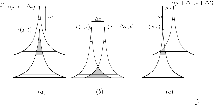
Figure 2: Spatio-temporal overlaps (shaded areas) of the ambit sets separated by a (a) temporal distance $\Delta t$, (b) spatial distance $\Delta x$ and (c) spatio-temporal distance $(\Delta x,\Delta t)$.

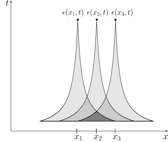
Figure 3: Illustration of the six disjoint contributions to the equal-time three-point correlation $\langle\varepsilon(x_{1},t)\varepsilon(x_{2},t)\varepsilon(x_{3},t)\rangle$.

Throwing many dice many times at different points in space is an example of an uncorrelated random process, because the number of points on a particular die is independent of those on other dice around it, and because the dice do not have any memory. Such uncorrelated random processes may seem unsuitable for describing correlated phenomena in nature. Lévy-based modelling, however, accomplishes exactly that. It does so by making use of overlapping sums of dice as follows: Suppose we have three dice labeled $A$, $B$ and $C$ whose outcomes are uncorrelated. The two variables $X=A+B$ and $Y=B+C$ will nevertheless be correlated since $X$ and $Y$ share the outcome of die $B$. This simple example can be generalised to construct correlated processes in spacetime. Let, for example, the energy $\varepsilon$ at a point $(x,t)$ be determined by the sum of outcomes of all dice occurring within its ambit set, a kind of causality cone similar to Einstein’s familiar light cone (see Figure 1). As shown in Figure 2, two energies at different points will then be correlated if their respective ambit sets overlap, because they will share a common ancestry to some extent. The freedom to choose both the kind of randomness and the form and size of the ambit set permits this approach to mimic different types of correlated behaviour. This article deals with the particular class of phenomena called multifractal and multiscaling, which includes turbulence, data traffic flows, cloud distributions, rain fields and tumour profiles, to name but a few. All of these show a power-law-like behaviour in their correlations which are easily incorporated into the Lévy-based modelling scheme by taking products of random variables rather than their sums. We show how to construct both the kind of randomness (the Lévy basis) and suitable ambit sets for this class, taking as input the measured correlations, and calculate analytically correlations for overlaps of various kinds (see Figures 2 and 3). While this paper concerns itself chiefly with multifractals, the Lévy scheme as such is much more general and can be appled to many other correlated random processes.

1 Introduction

Multifractality [1] has in the last decade become one of a number of well-established approaches to the analysis of time series and spatial patterns, whether nonlinear, random, deterministic, or chaotic. It serves, for example, to characterize the intermittent fluctuations observed in fully developed turbulent flows [2, 3] and in data traffic flows of communication networks [4]. Spatial patterns of cloud distributions and rain fields [5, 6] reveal multifractal properties, as do super-rough tumor profiles [7]. While still controversial, multiscaling has also been applied to financial time series of exchange rates and stock indices [8, 9, 10]. Many other examples may be found in the literature.

Multifractality should not, however, be seen as a mere tool for analysis and characterization: it has also found its way into theoretical modeling. Maybe the simplest construction of a multifractal field is achieved with random multiplicative cascade processes [2] which introduce a hierarchy of scales and multiplicatively redistribute a flux density from large to small scales.

Various generalizations of such purely spatial and discrete cascade processes towards continuous cascade processes in time and/or space, formulated in terms of integrals over an uncorrelated noise field, have been undertaken recently. A purely temporal and causal generalization to a continuous cascade process is, for example, discussed by Schmitt [11], who introduces a log-normal field, itself defined as an integral of a weighted and uncorrelated noise field over an associated time-dependent interval. By judicious choice of integration interval and weight function, the resulting process is stationary and exhibits approximate scaling behaviour of two-point correlations.

Muzy and Bacry [12] discuss a similar approach, constructing a purely temporal multifractal measure with the help of a limiting process. Since, however, the field amplitude depends on times later than the observation time $t$, the model does not obey causality.

The proper description and modeling of spatio-temporal multifractal physical processes clearly calls for a model generalization that is causal, explicitly depends on space and time and does so in a continuous framework. A first step in this direction was achieved in [13], where a continuous and causal spatio-temporal process was constructed in analogy to a discrete cascade process. Analytical forms for two- and three-point correlations for the case of a stable noise field were successfully compared to the corresponding experimental statistics in fully developed turbulent shear flow.

The aim of the work presented here is to provide a general framework for the construction of spatio-temporal processes that permits a unified description of the above-mentioned models [11, 12, 13] while transcending them all. The basic notion in this framework is that of independently scattered random measures of Lévy type. The appealing mathematics behind these measures, as described in [14] (with emphasis on spatio-temporal modeling), provide a characterisation of arbitrary $n$-point correlations independent of the choice of a concrete realisation of the model. This opens up the possibility of designing spatio-temporal processes almost to order, i.e. satisfying prescribed correlations.

As an application, we present the construction of a multiscaling and causal spatio-temporal process that is based on and derived from scaling two-point correlations. In contrast to [11] and [13], where the specification of the probability density of the noise-field must be included from the very beginning, we can construct the process without fixing the marginal distribution of the field-amplitude. This opens up the possibility of tailoring the marginal distribution of the process to the phenomenology of a given application. In particular, the special case of a stable law coincides with [13].

While we will concentrate on multifractal examples in most of this paper, it should be noted that this framework is not restricted to multiscaling (defined as scaling of correlation functions) or multifractal processes (defined as scaling of the coarse-grained process).

The paper is structured as follows. In Section 2, we discuss the general framework for spatio-temporal modeling and derive an explicit expression for $n$-point correlation functions for the general set-up. Based on this result, we turn to the application in the context of causal and multiscaling spatio-temporal processes in Section 3, where we show in detail the multiscaling properties of temporal and spatial $n$-point correlations of arbitrary order and establish a relation between spatio-temporal multiscaling and spatio-temporal multifractality. Section 4 concludes the paper with a summary and a brief outlook.

2 General model approach

The aim of this Section is to define the general framework and to provide useful mathematics for the construction of a class of causal spatio-temporal processes that are based on the integration of an independently scattered random measure of Lévy type. The integral constituting a given observable extends over a finite domain in space-time, called the ambit set $S$. This approach includes the special case of a continuous cascade process in space and/or time as an example. In particular, we recover the temporal cascade processes discussed in [11] and [12], as well as the spatio-temporal cascade process derived in [13]. In this paper, we restrict ourselves to causal processes in $1+1$ dimensions only, referring the reader to [14] and [15] for the general case of $(n{+}1)$-dimensional processes and its various applications and properties.

The basic notion is that of an independently scattered random measure (i.s.r.m) on continous space-time, $\mathbf{R}{\times}\mathbf{R}$. Loosely speaking, the measure associates a random number with any subset of $\mathbf{R}{\times}\mathbf{R}$. Whenever two subsets are disjoint, the associated measures are independent, and the measure of a disjoint union of sets almost certainly equals the sum of the measures of the individual sets. For a mathematically more rigorous definition of i.s.r.m.’s and their theory of integration, see Refs. [14, 16, 17].

Independently scattered random measures provide a natural basis for describing uncorrelated noise processes in space and time. A special class of i.s.r.m.’s is that of homogeneous Lévy bases, where the distribution of the measure of each set is infinitely divisible and does not depend on the location of the subset. In this case, it is easy to handle integrals with respect to the Lévy basis using the well-known Lévy-Khintchine and Lévy-Ito representations for Lévy processes. Here, we state the result and point to [14] for greater detail and rigour.

Let $Z$ be a homogeneous Lévy basis on $\mathbf{R}{\times}\mathbf{R}$, i.e. $Z(S)$ is infinitely divisible for any $S\subset\mathbf{R}{\times}\mathbf{R}$. Then we have the fundamental relation

$$\left\langle\exp\left\{\int_{S}h(a)Z(\mathrm{d}a)\right\}\right\rangle=\exp\left\{\int_{S}\mathrm{K}[h(a)]\mathrm{d}a\right\}\,,$$ (1)

where $\langle\cdots\rangle$ denotes the expectation, $h$ is any integrable deterministic function, and $\mathrm{K}$ denotes the cumulant function of $Z(\mathrm{d}a)$, defined by

$$\ln\left\langle\exp\left\{\xi Z(\mathrm{d}a)\right\}\right\rangle=\mathrm{K}[\xi]\,\mathrm{d}a.$$ (2)

The usefulness of (1) is obvious: it permits explicit calculation of the correlation function of the integrated and $h$-weighted noise field $Z(\mathrm{d}a)$ once the cumulant function $\mathrm{K}$ of $h$ is known.

2.1 General model ansatz

Based on relation (1), we construct a spatio-temporal process that is causal and continuous by defining the observable field $\epsilon(x,t)$ as

$$\epsilon(x,t)=\exp\left\{\int_{S(x,t)}h(x,t;x^{\prime},t^{\prime})Z(\mathrm{d}x^{\prime}{\times}\mathrm{d}t^{\prime})\right\}.$$ (3)

This is clearly a multiplicative process of independent factors $\exp\{h(x,t;x^{\prime},t^{\prime})\;Z(\mathrm{d}x^{\prime}{\times}\mathrm{d}t^{\prime})\}$ made up of a specifiable weight function $h$ and a homogeneous Lévy basis $Z$ over $\mathbf{R}{\times}\mathbf{R}$. Contributions to field amplitude $\epsilon(x,t)$ lie within the influence domain $S(x,t)$, called the associated ambit set. To guarantee causality, we demand that $S$ be nonzero only for times preceding the observation time $t$, i.e. $S(x,t)\subset\mathbf{R}{\times}[-\infty,t]$ (see Figure 1).

Ansatz (3) reduces to the model of Ref. [11] when focusing on one purely temporal dimension, setting $S(t)=[t+1-\lambda,t]$, $\lambda>1$, $h(t;t^{\prime})=(t-t^{\prime})^{-1/2}$ and defining $Z$ to be Brownian motion. Similarly, a non-causal and again purely temporal version of the general model (3) with a conical ambit set leads to the scale-dependent measures used in [12].

As shown in the Appendix and discussed in Section 3.4, our approach also includes the case of a multifractal measure that is constructed without a limit-argument. Moreover, it allows for multifractality in space and time simultaneously. This multifractal case (with the additional assumption of a stable Lévy basis) corresponds to the log-stable process described in [13], where the ambit set is constructed from an analogy to a cascade process. In Section 3.2, we derive the same result from an alternative approach.

Some other applications of (3) are discussed in [14].

The generality of the model (3) is based on the possibility of choosing the constituents of the process $\epsilon(x,t)$ independently. The available degrees of freedom are the weight function $h$, an arbitrary infinitely divisible distribution for the Lévy basis $Z$ (including Brownian motion, stable processes, self-decomposable processes etc.) and the shape of the ambit set $S$. As all of these quantities can be chosen to fit the purpose and application in mind, our ansatz permits sensitive and flexible modeling of the correlation structure of $\epsilon(x,t)$. Despite its generality, the model is tractable enough to yield explicit expressions for arbitrary $n$-point correlations in closed form.

2.2 n-point correlations

The definition of the process $\epsilon(x,t)$ allows for an explicit calculation of arbitrary spatio-temporal $n$-point correlations, defined as

$$c_{n}(x_{1},t_{1};\ldots;x_{n},t_{n})\equiv\left\langle\epsilon(x_{1},t_{1})\cdot\ldots\cdot\epsilon(x_{n},t_{n})\right\rangle\,,$$ (4)

which give a complete characterisation of the correlation structure of $\epsilon(x,t)$.

Using the definition (3) and the fundamental relation (1) we rewrite

$$c_{n}(x_{1},t_{1};\ldots;x_{n},t_{n})=$$ (5)

$$= \left\langle\exp\left\{\sum_{i=1}^{n}\int_{S(x_{i},t_{i})}h(x_{i},t_{i};x^{\prime},t^{\prime})Z(\mathrm{d}x^{\prime}{\times}\mathrm{d}t^{\prime})\right\}\right\rangle$$

$$= \left\langle\exp\left\{\int_{\mathbf{R}{\times}\mathbf{R}}\left(\sum_{i=1}^{n}\mathrm{I}_{S(x_{i},t_{i})}h(x_{i},t_{i};x^{\prime},t^{\prime})\right)Z(\mathrm{d}x^{\prime}{\times}\mathrm{d}t^{\prime})\right\}\right\rangle$$

$$= \exp\left\{\int_{\mathbf{R}{\times}\mathbf{R}}\mathrm{K}\left[\left(\sum_{i=1}^{n}\mathrm{I}_{S(x_{i},t_{i})}h(x_{i},t_{i};x^{\prime},t^{\prime})\right)\right]\mathrm{d}x^{\prime}\mathrm{d}t^{\prime}\right\},$$

where we made use of the index-function

$$\mathrm{I}_{A}(x,t)=\left\{\begin{array}[]{ll}1&\mathrm{when\ }(x,t)\in A\\ &\\ 0&\mathrm{otherwise}\end{array}\right.$$ (6)

for sets $A\subset\mathbf{R}{\times}\mathbf{R}$. The last step in (5) follows from the fundamental equation (1).

To illustrate (5), we consider in more detail the cases $n=2$ and $n=3$ with the abbreviation $S_{i}=S(x_{i},t_{i})$. For $n=2$, it follows that

$$\left\langle\epsilon(x_{1},t_{1})\epsilon(x_{2},t_{2})\right\rangle = \exp\left\{\int_{S_{1}\backslash S_{2}}\mathrm{K}\left[h(x_{1},t_{1};x,t)\right]\mathrm{d}x\,\mathrm{d}t\right\}$$ (7)

$$\times \exp\left\{\int_{S_{2}\backslash S_{1}}\mathrm{K}\left[h(x_{2},t_{2};x,t)\right]\mathrm{d}x\,\mathrm{d}t\right\}$$

$$\times \exp\left\{\int_{S_{1}\cap S_{2}}\mathrm{K}\left[h(x_{1},t_{1};x,t)+h(x_{2},t_{2};x,t)\right]\mathrm{d}x\,\mathrm{d}t\right\}.$$

As illustrated in Figure 2.c, the first and second factor are contributions from the non-overlapping parts of the ambit sets, while the third stems from the overlap of $S(x_{1},t_{1})$ and $S(x_{2},t_{2})$ (the shaded area). The latter factor describes the correlation of the field amplitude $\epsilon$ at different spatio-temporal locations; for locations where the overlap $S(x_{1},t_{1})\cap S(x_{2},t_{2})$ vanishes, we get uncorrelated field amplitudes $\langle\epsilon(x_{1},t_{1})\epsilon(x_{2},t_{2})\rangle-\langle\epsilon(x_{1},t_{1})\rangle\langle\epsilon(x_{2},t_{2})\rangle=0$. Thus, the extension and shape of $S(x,t)$ characterises the range of correlations, while the overlap of two ambits, the weight-function $h$ and the cumulant function $\mathrm{K}$ influences the correlation strength.

In third order we get a similar result. The combinatorics of the overlap of ambit sets for the observation points $(x_{1},t_{1})$, $(x_{2},t_{2})$ and $(x_{3},t_{3})$ yields seven disjoint domains as follows: the three domains $S(x_{1},t_{1})\backslash[S(x_{2},t_{2})\cup S(x_{3},t_{3})]$, $S(x_{2},t_{2})\backslash[S(x_{1},t_{1})\cup S(x_{3},t_{3})]$ and $S(x_{3},t_{3})\backslash[S(x_{1},t_{1})\cup S(x_{2},t_{2})]$ give uncorrelated contributions associated solely with one field amplitude; for instance, $S(x_{1},t_{1})\backslash[S(x_{2},t_{2})\cup S(x_{3},t_{3})]$ is the contribution to $\epsilon(x_{1},t_{1})$ that is independent of $\epsilon(x_{2},t_{2})$ and $\epsilon(x_{3},t_{3})$. A second set of three domains $[S(x_{1},t_{1})\cap S(x_{2},t_{2})]\backslash S(x_{3},t_{3})$, $[S(x_{1},t_{1})\cap S(x_{3},t_{3})]\backslash S(x_{2},t_{2})$ and $[S(x_{2},t_{2})\cap S(x_{3},t_{3})]\backslash S(x_{1},t_{1})$ constitute the contributions to the correlation of two field amplitudes but without that of the third field amplitude. Finally, $S(x_{1},t_{1})\cap S(x_{2},t_{2})\cap S(x_{3},t_{3})$ is the overlap of all three ambit sets that describes the common correlation of all three field amplitudes.

Using the simplified notation $\mathrm{K}_{i_{1},i_{2}.\ldots,i_{j}}\equiv\mathrm{K}[h(x_{i_{1}},t_{i_{1}};x,t)+h(x_{i_{2}},t_{i_{2}};x,t)+\cdots+h(x_{i_{j}},t_{i_{j}};x,t)]$, the result in third order hence reads

$$\left\langle\epsilon(x_{1},t_{1})\epsilon(x_{2},t_{2})\epsilon(x_{3},t_{3})\right\rangle=$$ (8)

$$= \exp\left\{\int_{S_{1}\backslash(S_{2}\cup S_{3})}\!\!\!\!\!\mathrm{K}_{1}\,\mathrm{d}x\,\mathrm{d}t\right\}\exp\left\{\int_{S_{2}\backslash(S_{1}\cup S_{3})}\!\!\!\!\!\mathrm{K}_{2}\,\mathrm{d}x\,\mathrm{d}t\right\}\exp\left\{\int_{S_{3}\backslash(S_{1}\cup S_{2})}\!\!\!\!\!\mathrm{K}_{3}\,\mathrm{d}x\,\mathrm{d}t\right\}$$

$$\times \exp\left\{\int_{(S_{1}\cap S_{2})\backslash S_{3}}\!\!\!\!\!\mathrm{K}_{1,2}\,\mathrm{d}x\,\mathrm{d}t\right\}\exp\left\{\int_{(S_{1}\cap S_{3})\backslash S_{2}}\!\!\!\!\!\mathrm{K}_{1,3}\,\mathrm{d}x\,\mathrm{d}t\right\}\exp\left\{\int_{(S_{2}\cap S_{3})\backslash S_{1}}\!\!\!\!\!\mathrm{K}_{2,3}\,\mathrm{d}x\,\mathrm{d}t\right\}$$

$$\times \exp\left\{\int_{S_{1}\cap S_{2}\cap S_{3}}\!\!\!\!\!\mathrm{K}_{1,2,3}\,\mathrm{d}x\,\mathrm{d}t\right\}\,.$$

It is clear from the above examples that the correlation structure corresponds directly to an intuitive geometrical picture in which the design and the overlap of the ambit sets $S$ determine the correlation structure.

Conversely, one can use some given correlation structure $c_{n}$ as the starting point for designing a suitable shape of the ambit set and weight-function $h$ to fit these requirements, opening up a wide range of applications. As outlined in the next section, multiscaling appears as a specific example, while Ref. [14] provides further insight into the kind of processes that can be modeled and explores the potential of the additive counterpart defined as $\ln\epsilon(x,t)$).

3 Multiscaling model specifications

In this Section, the concept of multiscaling and multifractality is examined in the context of the general model approach presented above. An explicit expression for the ambit set $S$ is derived from scaling two-point correlations, and fusion rules [18] expressing $n$-point correlations solely in terms of scaling relations are formulated. Finally, the link to standard multifractality is established.

3.1 General remarks and assumptions

In order to keep the mathematics as transparent as possible, we will use some simplifying assumptions about the structure of the process $\epsilon(x,t)$. Our goal is the construction of a stationary and translationally invariant process with scaling two-point correlations. For the simplest way to achieve stationarity and translational invariance, we assume $h\equiv 1$ and take the form of the ambit set $S(x,t)$ to be independent of the location $(x,t)$, so that

$$S(x,t)=(x,t)+S_{0}\,,$$ (9)

where the shape of $S_{0}$ is independent of $(x,t)$. (Note that $h\equiv 1$ is not a prerequisite for stationarity and translational invariance. It would be sufficient to require $h(x^{\prime},t^{\prime};x,t)\equiv h(x^{\prime},t^{\prime})$, but we can do without this additional degree of freedom for the special case of scaling relations for two-point correlations.)

Figure 1 illustrates the various features of $S(x,t)$, which we now discuss. At the origin $(0,0)$, it is specified mathematically by

$$S_{0}=\left\{(x,t)\in\mathbf{R}{\times}\mathbf{R}:-T\leq t\leq 0,-g(t+T)\leq x\leq g(t+T)\right\}.$$ (10)

This definition contains a finite decorrelation time $T$, ensuring that no correlation survives for temporal separations $\Delta t$ larger than $T$, e.g. $\langle\epsilon(x,t)\epsilon(x,t+\Delta t)\rangle-\langle\epsilon(x,t)\rangle\langle\epsilon(x,t+\Delta t)\rangle=0$ for all $\Delta t\geq T$.

Spatially, the ambit $S_{0}$ is limited by a function $g(t)$, whose monotonicity ensures that the spatial extension of the causality domain increases monotonically for past times. The nonconstancy of $g$ implies a time-dependent spatial decorrelation length $l(\Delta t)$, since, when two observations are separated by a space-time distance $(\Delta x,\Delta t)$ (as illustrated in Figure 2.c), the two-point correlation $\langle\epsilon(x,t)\epsilon(x+\Delta x,t+\Delta t)\rangle-\langle\epsilon(x,t)\rangle\langle\epsilon(x+\Delta x,t+\Delta t)\rangle$ vanishes for all $\Delta x\geq l(\Delta t)=g(\Delta t)+g(0)$. The spatial decorrelation length $l(\Delta t)$ decreases monotonically with $\Delta t$, and its maximum $l(0)=2g(0)\equiv L$ defines the decorrelation length $L$. This is a physically desirable property.

Finally, we impose a locality condition $g(T)=0$, i.e. the ambit set $S_{0}$ is attached to $(x,t)$ in an unequivocal way.

The procedure followed in the next section starts from the assumption that spatial and temporal two-point correlations scale, and constructs the model according to this requirement. The basic relation we use in the translationally invariant and stationary case under the assumptions (9) and $h\equiv 1$ is

$$\langle\epsilon(x,t)\epsilon(x+\Delta x,t+\Delta t)\rangle$$ (11)

$$= \exp\left\{\int_{S_{1}\backslash S_{2}}\mathrm{K}[1]\mathrm{d}x\,\mathrm{d}t\right\}\exp\left\{\int_{S_{2}\backslash S_{1}}\mathrm{K}[1]\mathrm{d}x\,\mathrm{d}t\right\}\exp\left\{\int_{S_{1}\cap S_{2}}\mathrm{K}[2]\mathrm{d}x\,\mathrm{d}t\right\}$$

$$= \exp\left\{\int_{S_{1}}\mathrm{K}[1]\mathrm{d}x\,\mathrm{d}t\right\}\exp\left\{\int_{S_{2}}\mathrm{K}[1]\mathrm{d}x\,\mathrm{d}t\right\}\exp\left\{\int_{S_{1}\cap S_{2}}(\mathrm{K}[2]-2\mathrm{K}[1])\mathrm{d}x\,\mathrm{d}t\right\}$$

$$= \langle\epsilon\rangle^{2}\exp\biggr{\{}V(\Delta x,\Delta t)(\mathrm{K}[2]-2\mathrm{K}[1])\biggr{\}}\,,$$

where we have used (7) with $h\equiv 1$ and the abbreviations $S_{1}=S(x,t)$, $S_{2}=S(x+\Delta x,t+\Delta t)$ and

$$V(\Delta x,\Delta t)=\mathrm{Vol}(S(x,t)\cap S(x+\Delta x,t+\Delta t))$$ (12)

for the Euclidean volume of the overlap of the ambit sets. Due to translational invariance and stationarity, we have $\langle\epsilon(x,t)\rangle=\langle\epsilon(x+\Delta x,t+\Delta t)\rangle=\langle\epsilon\rangle$.

Assuming that $\mathrm{K}[2]>2\mathrm{K}[1]$ (note that, by the strict convexity of log-Laplace transforms, we always have $\mathrm{K}[2]-2\mathrm{K}[1]\geq 0$), Eq. (11) can be solved for $V$,

$$V(\Delta x,\Delta t)=\frac{1}{\mathrm{K}[2]-2\mathrm{K}[1]}\;\;{\ln\left({\displaystyle\frac{\langle\epsilon(x,t)\epsilon(x+\Delta x,t+\Delta t)\rangle}{\langle\epsilon\rangle^{2}}}\right)}.$$ (13)

This relation establishes a simple geometrical way to design a model with prescribed two-point correlations: one has only to choose ambit sets $S(x,t)$ in a way that the volume of the overlap fulfils (13). This will be done in the next Section for the case of scaling two-point correlations (see [14] for more examples other than scaling relations).

3.2 Construction of the ambit set via scaling two-point correlations

Implementing the general framework (3) together with the above assumptions and procedure, we start out by demanding power-law scaling for the lowest-order spatial and temporal correlations,

$$\left\langle\epsilon(x,t)\epsilon(x+\Delta x,t)\right\rangle=c_{x}(\Delta x)^{-\tau(2)},\;\;\;\Delta x\in[l_{scal},L_{scal}]\subset[0,L],$$ (14)

$$\left\langle\epsilon(x,t)\epsilon(x,t+\Delta t)\right\rangle=c_{t}(\Delta t)^{-\tau(2)},\;\;\;\Delta t\in[t_{scal},T_{scal}]\subset[0,T],$$ (15)

with $c_{x}$ and $c_{t}$ constants. Note that the scaling exponents $\tau(2)$ appearing in (14) and (15) are taken to be identical; differing spatial and temporal scaling exponents, as used previously e.g. in [15], are easily accommodated within our model, but do not satisfy the simpler relations (18) given below.

Following the recipe sketched in (13), we get, using stationarity, for the temporal two-point correlation (15) the expression (see Figures 1 and 2.a)

$$V(0,\Delta t) = \int_{\Delta t}^{T}2g(t)\mathrm{d}t\ =\int_{\Delta t}^{T-T_{scal}}2g(t)\mathrm{d}t\ +\int_{T-T_{scal}}^{T}2g(t)\mathrm{d}t$$ (16)

$$= \frac{\ln c_{t}-\ln(\langle\epsilon\rangle^{2})}{\mathrm{K}[2]-2\mathrm{K}[1]}-\frac{\tau(2)\ln\Delta t}{\mathrm{K}[2]-2\mathrm{K}[1]}$$

for $\Delta t\in[t_{scal},T_{scal}]$, and after differentiation of both sides with respect to $\Delta t$, we obtain the expression

$$g(t)=\frac{\tau(2)}{2(\mathrm{K}[2]-2\mathrm{K}[1])}\frac{1}{t},\;\;\;\;\;t\in[t_{scal},T_{scal}]$$ (17)

for the function $g(t)$ bounding the ambit set $S(x,t)$ within the temporal scaling regime $[t_{scal},T_{scal}]$. The singularity of $g(t)$ for $t\to 0$ and the locality condition $g(T)=0$ retrospectively justify the introduction of the cutoffs $t_{scal}$ and $T_{scal}$ for the temporal scaling regime. We could also have started from the spatial scaling relation (14) to obtain exactly the same functional form for $g(t)$ with

$$g(T_{scal})=\frac{l_{scal}}{2},\;\;\;g(t_{scal})=\frac{L_{scal}}{2}.$$ (18)

Thus the set of scaling relations (14) and (15) are compatible under the assumption of a constant weight-function $h\equiv 1$, i.e. there exists a solution for $g(t)$ that satisfies (14) and (15) simultaneously. This sheds some light on the property of the weight-function $h$ to select compatible temporal and spatial two-point correlations: scaling relations are among the simplest functional forms and allow $h\equiv 1$, while for more advanced studies, such as deviations from scaling for $\Delta t\notin[t_{scal},T_{scal}]$ and $\Delta x\notin[l_{scal},L_{scal}]$, other weight-functions $h$ might be in order. For a brief account of this topic we refer the reader to [14].

To complete the specification of $g(t)$, functional forms in the time intervals $0\leq t\leq t_{scal}$ and $T_{scal}\leq t\leq T$ are needed in principle. For this analytical treatise, however, it is not necessary to specify the functional form of $g(t)$ explicitly for these two time intervals, since we neglect the constants of proportionality $c_{x}$ and $c_{t}$ in (14) and (15) in any case; examples addressing this issue can be found in Ref. [15]. The important point is that the validity of the scaling relations (14) and (15) is independent of a specific choice of $g(t)$ for $t\notin[t_{scal},T_{scal}]$: Figure 1 and Figure 2.a show that, for purely temporal separation, spatial scales in $S$ larger than $L_{scal}$ do not contribute to the ambit overlap $S_{1}\cap S_{2}$ for $\Delta t>t_{scal}$, while spatial scales in $S$ smaller than $l_{scal}$ are completely part of the overlap for $\Delta t<T_{scal}$ and thus contribute only a term constant in $\Delta t$.

Similar results hold for the purely spatial separation shown in Figure 2.b: regions of $S$ smaller than $l_{scal}$ do not contribute to the overlap for $\Delta x>l_{scal}$. The contributions from the large scales $>L_{scal}$ result in a constant, as can easily be seen from

$$V(\Delta x,0) = \int_{0}^{g^{(-1)}(\Delta x/2)}\left(2g(t)-\Delta x\right)\mathrm{d}t$$ (19)

$$= \int_{0}^{t_{scal}}2g(t)\mathrm{d}t\ +\int_{t_{scal}}^{g^{(-1)}(\Delta x/2)}2g(t)\mathrm{d}t\ -\frac{\tau(2)}{\mathrm{K}[2]-2\mathrm{K}[1]},$$

where $g^{(-1)}$ denotes the inverse of $g$. Thus, a specific choice of $g(t)$ for $t<t_{scal}$ only involves the constant $c_{x}$ and does not influence the scaling behaviour (14) as such. The only restriction is $V(0,0)<\infty$ (for finite expectations).

3.3 Structure of higher-order correlations

In the previous Section, we specified the model starting from scaling two-point correlations. It is now straightforward to derive scaling relations for all higher order correlations of purely spatial and temporal type. Section 3.4 shows how these scaling relations imply multifractality.

First we note that, since $h\equiv 1$, equation (5) translates to

$$c_{n}(x_{1},t_{1};\ldots;x_{n},t_{n})=\exp\left\{\int_{\mathbf{R}{\times}\mathbf{R}}\mathrm{K}\left[\sum_{i=1}^{n}\mathrm{I}_{S(x_{i},t_{i})}(x,t)\right]\mathrm{d}x\,\mathrm{d}t\right\}.$$ (20)

The argument of the cumulant function $\mathrm{K}$ in (20) is piecewise constant where $\sum_{i=1}^{n}\mathrm{I}_{S(x_{i},t_{i})}(x,t)$ counts the number of field amplitudes $\epsilon(x_{i},t_{i})$ that contribute to $(x,t)$ via their ambit sets $S(x_{i},t_{i})$. This function vanishes outside of $\bigcup_{i=1}^{n}S(x_{i},t_{i})$.

Focusing first on purely spatial two-point correlations of higher order, we get, using (20), the analog to (11)

$$\left\langle\epsilon(x,t)^{n_{1}}\epsilon(x+\Delta x,t)^{n_{2}}\right\rangle = \left\langle\epsilon(x,t)^{n_{1}}\right\rangle\left\langle\epsilon(x+\Delta x,t)^{n_{2}}\right\rangle$$ (21)

$$\times \exp\left\{V(\Delta x,0)\left(\mathrm{K}[n_{1}+n_{2}]-\mathrm{K}[n_{1}]-\mathrm{K}[n_{2}]\right)\right\}.$$

Translational invariance and (17), (19) imply scaling relations for the higher-order two-point correlations

$$\left\langle\epsilon(x,t)^{n_{1}}\epsilon(x+\Delta x,t)^{n_{2}}\right\rangle\propto(\Delta x)^{-\tau(n_{1},n_{2})},\;\;\;\Delta x\in[l_{scal},L_{scal}],$$ (22)

where

$$\tau(n_{1},n_{2})=\frac{\tau(2)}{\mathrm{K}[2]-2\mathrm{K}[1]}\biggr{(}\mathrm{K}[n_{1}+n_{2}]-\mathrm{K}[n_{1}]-\mathrm{K}[n_{2}]\biggr{)}.$$ (23)

(Again, the convexity of $\mathrm{K}$ implies $\mathrm{K}[n_{1}+n_{2}]-\mathrm{K}[n_{1}]-\mathrm{K}[n_{2}]\geq 0$.) The scaling range of (22) is identical to the scaling range of (14) and does not depend on the order $(n_{1},n_{2})$.

An analogous procedure leads to scaling relations for the spatial higher-order three-point correlations illustrated in Figure 3. For ordered points $x_{1}<x_{2}<x_{3}$ with relative distances assumed to be within the spatial scaling range, $|x_{i}-x_{j}|\in[l_{scal},L_{scal}]$, $(i,j=1,2,3)$, we find that

$$\left\langle\epsilon(x_{1},t)^{n_{1}}\epsilon(x_{2},t)^{n_{2}}\epsilon(x_{3},t)^{n_{3}}\right\rangle$$ (24)

$$\propto \left(x_{2}-x_{1}\right)^{-\tau(n_{1},n_{2})}\left(x_{3}-x_{2}\right)^{-\tau(n_{2},n_{3})}\left(x_{3}-x_{1}\right)^{-\xi(n_{1},n_{2},n_{3})}\,,$$

with a modified exponent $\xi$ defined by

$$\xi(n_{1},n_{2},n_{3})=\tau(n_{1}+n_{2},n_{3})-\tau(n_{2},n_{3})\;.$$ (25)

The reason for the different forms of the exponents $\tau$ and $\xi$ lies, of course, in the different ambit set overlaps: as shown in Figure 3, points $x_{1}$ and $x_{3}$ have only the one neighbour $x_{2}$, while $x_{2}$ has two.

Equation (24) can be viewed as a generalised fusion rule in the sense of [18]. It is easily generalised to $n$-point correlations of arbitrary order because all overlapping ambit sets can be written as a combination of overlaps $V(|x_{i}-x_{j}|,0)\propto\ln|x_{j}-x_{i}|$, as long as $|x_{i}-x_{j}|\in[l_{scal},L_{scal}]$ for all point pairs. As shown by induction in [15], the spatial $n$-point correlation for ordered points $x_{1}<x_{2}<\ldots<x_{n}$ and arbitrary order $(m_{1},\ldots,m_{n})$ satisfying $x_{i+1}-x_{i}\in[l_{scal},L_{scal}]$ has the following structure:

$$\left\langle\epsilon(x_{1},t)^{m_{1}}\cdots\epsilon(x_{n},t)^{m_{n}}\right\rangle$$ (26)

$$\propto \left(\prod_{i=1}^{n-1}\left(x_{i+1}-x_{i}\right)^{-\tau(m_{i},m_{i+1})}\right)\prod_{j=2}^{n-1}\prod_{l=j+1}^{n}\left(x_{l}-x_{l-j}\right)^{-\xi(m_{l-j},\ldots,m_{l})},$$

where

$$\xi(m_{l-j},\ldots,m_{l})=\tau(m_{l-j}+\ldots+m_{l-1},m_{l})-\tau(m_{l-j+1}+\ldots+m_{l-1},m_{l})\,.$$ (27)

The modified scaling-exponents $\xi(m_{1},\ldots,m_{j})$ correspond to (25) for $j=3$ and arise from the nested structure of the overlapping ambit sets. Physically, Eq. (26) implies that spatial $n$-point correlations factorise into contributions arising at the smallest scales $x_{i+1}-x_{i}$, at next-to-smallest scales $x_{i+2}-x_{i}$, and so on up to the largest scale, $x_{n}-x_{1}$.

To complete the discussion of $n$-point correlations, we state the corresponding relation for temporal $n$-point correlations of arbitrary order

$$\left\langle\epsilon(x,t_{1})^{m_{1}}\cdots\epsilon(x,t_{n})^{m_{n}}\right\rangle$$ (28)

$$\propto \left(\prod_{i=1}^{n-1}\left(t_{i+1}-t_{i}\right)^{-\tau(m_{i},m_{i+1})}\right)\prod_{j=2}^{n-1}\prod_{l=j+1}^{n}\left(t_{l}-t_{l-j}\right)^{-\xi(m_{l-j},\ldots,m_{l})}\;,$$

for ordered times $t_{1}<\ldots<t_{n}$ and $|t_{i}-t_{j}|\in[t_{scal},T_{scal}]$, $i,j=1,\ldots,n$. Finally it is to be noted that relations (26) and (28) only hold for purely spatial and purely temporal $n$-point correlations respectively. The general case of arbitrary $n$-point correlations (20) does not allow a similar description in terms of scaling relations, since $V(\Delta x,\Delta t)$ includes mixed terms in $\Delta x$ and $\Delta t$. For a complete discussion of general space-time two-point correlations, we refer again to [15].

3.4 Link to classical multifractality

We complete the discussion of the multiscaling model with an investigation of the relation between multiscaling (defined as scaling of $n$-point correlations (26) and (28)) and classical multifractality (defined as scaling of coarse-grained moments). In the Appendix, we prove that multiscaling implies multifractality in the large scale limit.

The term multifractality in the classical sense refers to $n$-th order moments of the field, coarse-grained at scale $l$ centered on locations $\sigma$, displaying scaling behaviour with some non-linear multifractal scaling exponent $\mu(n)>0$,

$$M_{n}(\sigma,l)=\left\langle\left(\frac{1}{l}\int_{\sigma-l/2}^{\sigma+l/2}\epsilon(\sigma^{\prime})\mathrm{d}\sigma^{\prime}\right)^{n}\right\rangle\propto l^{-\mu(n)}.$$ (29)

Note that this relation applies to stationary processes $\epsilon(\sigma)$ since the right hand side of (29) is independent of the location $\sigma$. Differentiating this relation twice with respect to $l$, it follows in second order, due to stationarity, that the two-point correlations

$$\left\langle\epsilon(\sigma+l)\epsilon(\sigma)\right\rangle\propto l^{-\mu(2)}$$ (30)

scale with the same scaling exponent $\mu(2)$ as $M_{2}$. The inverse need not be true, for the scaling relation (30) becomes singular for $l\rightarrow 0$, though at small scales deviations from (30) have to occur which in turn may destroy the relation (29) [19, 20]. However, (30) indicates a strong connection between scaling of $n$-point correlations and multifractal scaling of order $n$.

The multiscaling model implies scaling relations for $n$-point correlations, with deviations from pure scaling for scales smaller than $l_{scal}$ for spatial correlations and scales smaller than $t_{scal}$ for temporal ones. Thus the question arises whether multifractal exponents $\mu(n)$ are to be expected (see also [15]). To answer this question, we assume the one-point moments $\langle\epsilon(x,t)^{n}\rangle$ to be finite (i.e. we restrict to Lévy bases with $\mathrm{K}[n]<\infty$).

In the Appendix it is shown that the integral moments of temporal type

$$M^{(t)}_{n}(t,l)=\left\langle\left(\frac{1}{l}\int_{t-l/2}^{t+l/2}\epsilon(x,t^{\prime})\mathrm{d}t^{\prime}\right)^{n}\right\rangle\propto l^{-\mu(n)}$$ (31)

asymptotically exhibit scaling behaviour for $t_{scal}\ll l$. Moreover this is also true for the integral moments of spatial type

$$M^{(s)}_{n}(x,l)=\left\langle\left(\frac{1}{l}\int_{x-l/2}^{x+l/2}\epsilon(x^{\prime},t)\mathrm{d}x^{\prime}\right)^{n}\right\rangle\propto l^{-\mu(n)}$$ (32)

for $l_{scal}\ll l$ with the same multifractal scaling exponents

$$\mu(n)=\frac{\tau(2)}{\mathrm{K}[2]-2\mathrm{K}[1]}(\mathrm{K}[n]-n\mathrm{K}[1]).$$ (33)

The crucial assumption that enters the proof of (31) and (32) is

$$\tau(2)\frac{\mathrm{K}[n]-\mathrm{K}[n-1]-\mathrm{K}[1]}{\mathrm{K}[2]-2\mathrm{K}[1]}=\mu(n)-\mu(n-1)<1.$$ (34)

This assumption ensures that large scale correlations dominate the moments of the coarse grained field. It is to note that (34) is a sufficient condition for multifractality in the large-scale limit. The statistics of the energy dissipation in fully developed turbulence is an important example of an observable where condition (34) holds; see Ref. [21].

The identity of spatial and temporal multifractal scaling exponents $\mu(n)$ is clearly a result of the identical scaling behaviour of purely spatial and temporal $n$-point correlations. The scaling of spatial and temporal integral moments is independent of the choice of the boundary function $g(t)$ for $t\notin[t_{scal},T_{scal}]$ as long as $V(0,0)<\infty$. Under these mild restrictions, we are able to model a wide range of scaling exponents $\mu(n)$ by choosing a proper cumulant function $\mathrm{K}$ via the Lévy basis $Z$ that fulfils the sufficient condition (34). Examples are $\mu(n)\propto n^{\alpha}-n$ for a stable basis with index of stability $0<\alpha\leq 2$, $\alpha\neq 1$ and

$$\mu(n)\propto(1-n)\sqrt{\alpha^{2}-\beta^{2}}+n\sqrt{\alpha^{2}-(\beta+1)^{2}}-\sqrt{\alpha^{2}-(\beta+n)^{2}},$$ (35)

with $|\beta+n|\leq\alpha$, for a normal-inverse-Gaussian distribution $\mathrm{NIG}(\alpha,\beta,\delta,\nu)$ [22, 23, 24]. Depending on the parameters that characterize the distributions, there exists a critical order $n_{c}$ where (34) does not hold any more. The $\mathrm{NIG}(\alpha,\beta,\delta,\nu)$ distribution is an example of a Lévy basis where multifractality (29) is defined only up to a finite order $n$, since $\mathrm{K}[n]<\infty$ only for $|\beta+n|\leq\alpha$; for larger $n$, the moments $\langle\epsilon^{n}\rangle$ and $M_{n}$ do not exist.

4 Conclusion

We have presented a general framework for modeling of spatio-temporal processes that allows, even in its generality, an analytical treatment of general spatio-temporal $n$-point correlations. This framework consists of a homogeneous Lévy basis, the concept of an ambit set as an associated influence domain and a weight-function $h$. These three degrees of freedom can be chosen arbitrarily and independently, thus encompassing a wide range of applications. In this respect, we mentioned briefly related work [11, 12, 13] and showed them to be special cases of this framework. In a specific illustration, we have shown that a stationary and translationally invariant version of the general model can be used to construct a multiscaling and multifractal causal spatio-temporal process starting from scaling relations of two-point correlations.

Many applications immediately come to mind. The great flexibility and tractability of the framework’s mathematics might well find its way into modeling of rainfields, cloud distributions and various growth models, to name just a few examples of spatio-temporal processes. Another field of application for the special case of the multiscaling model is the description and modeling of the statistics of the energy-dissipation in fully developed turbulence as a prototype of a multifractal and multiscaling field. A first step in this direction was undertaken in [13], where scaling two- and three-point correlations (15) and (28) were shown to be in excellent correspondence with data extracted from a turbulent shear flow experiment.

Appendix: Scaling relations for integral moments

This appendix proves the classical multifractal property (29) for the multiscaling model in the limit $t_{scal}\ll t\leq T_{scal}$ and $l_{scal}\ll l\leq L_{scal}$ under the assumption that

$$\tau(2)\frac{\mathrm{K}[n]-\mathrm{K}[n-1]-\mathrm{K}[1]}{\mathrm{K}[2]-2\mathrm{K}[1]}<1.$$ (36)

The proof is carried out in detail only for the spatial case; the temporal counter part of the above statement is straightforward.

With the abbreviation $d_{n}(l_{2},\ldots,l_{n})=\langle\epsilon(0,t)\epsilon(l_{2},t)\cdots\epsilon(l_{n},t)\rangle$ , $0<l_{2}<\ldots l_{n}$ for the spatial correlation function of order $n$ and using the translational invariance of the correlation structure, the spatial integral moments of order $n$ (32) are given by

$$M_{n}^{(s)}(x,l)=n!\;l^{-n}\int_{0}^{l}\mathrm{d}l_{n}\int_{0}^{l_{n}}\mathrm{d}l_{n-1}\cdots\int_{0}^{l_{3}}\mathrm{d}l_{2}\left(l-l_{n}\right)d_{n}\;(l_{2},\ldots,l_{n}).$$ (37)

To calculate the involved overlaps of the influence domains, it must be distinguished whether the spatial distances are smaller or larger than $l_{scal}$. In the limit $l_{scal}\ll l$, the dominant contribution is

$$M_{n}^{(s)}(x,l)\approx\tilde{M}_{n}^{(s)}(l)$$

$$= n!\;l^{-n}\int_{(n-1)l_{scal}}^{l}dl_{n}\int_{(n-2)l_{scal}}^{l_{n}-l_{scal}}dl_{n-1}\cdots\int_{l_{scal}}^{l_{3}-l_{scal}}dl_{2}\;\left(l-l_{n}\right)d_{n}(l_{2},\ldots,l_{n}).$$

The proof of the multifractality of $M_{n}^{(s)}(x,l)$ is carried out in two steps. The first part shows that $\tilde{M}_{n}^{(s)}(l)\propto l^{-\mu(n)}$ in the large scale limit. In the second step, we show that the approximation $M_{n}^{(s)}(x,l)\approx\tilde{M}_{n}^{(s)}(l)$ holds for $l\gg l_{scal}$. We also provide a rough estimate for the relative error $|M_{n}^{(s)}(x,l)-\tilde{M}_{n}^{(s)}(l)|/\tilde{M}_{n}^{(s)}(l)$.

The correlation function $d_{n}$ can be rewritten with the help of the generalised fusion rules (26) as

$$d_{n}(l_{2},\ldots,l_{n})\propto\prod_{k=2}^{n}\prod_{j=1}^{k-1}\left(l_{k}-l_{k-j}\right)^{-\xi_{j+1}}$$ (39)

where

$$\xi_{j+1}=\xi(\underbrace{1,\ldots,1}_{j-\rm{times}})$$ (40)

and $\xi_{2}\equiv\tau(1,1)$. In the next step, we define

$$F_{n}(l,l_{scal})$$

$$\equiv l^{-n}\int_{(n-1)l_{scal}}^{l}dl_{n}\int_{(n-2)l_{scal}}^{l_{n}-l_{scal}}dl_{n-1}\cdots\int_{l_{scal}}^{l_{3}-l_{scal}}dl_{2}\left(l-l_{n}\right)\prod_{k=2}^{n}\prod_{j=1}^{k-1}\left(l_{k}-l_{k-j}\right)^{-\xi_{j+1}}.$$

Note that $\tilde{M}_{n}(l)\propto F_{n}(l,l_{scal})$ with a constant of proportionality that is independent of $l$.

With the abbreviation

$$h(k)=-\sum_{j=1}^{k-1}\xi_{j+1},$$ (42)

it follows from (25 and (27) that

$$\sum_{k=2}^{n}h(k)=-\mu(n)$$ (43)

where

$$\mu(n)=\tau(2)\frac{\mathrm{K}[n]-n\mathrm{K}[1]}{\mathrm{K}[2]-2\mathrm{K}[1]}.$$ (44)

Thus we get, using condition (36)

$$h(n)=\mu(n-1)-\mu(n)=-\tau(2)\frac{\mathrm{K}[n]-\mathrm{K}[n-1]-\mathrm{K}[1]}{\mathrm{K}[2]-2\mathrm{K}[1]}>-1.$$ (45)

It follows immediately that

$$\tilde{M}_{n}\,(l)l^{\mu(n)}\propto F_{n}(1,l_{scal}/l).$$ (46)

$F_{n}(1,l_{scal}/l)$ is positive and increasing with increasing $l$. It is easy to show that $F_{n}(1,l_{scal}/l)$ is bounded. From (39) and (42) it follows that $d_{n}<\prod_{k=2}^{n}l_{k}^{h(k)}$ and therefore

$$F_{n}(1,l/l_{scal})<\int_{l_{scal}/l}^{1}\mathrm{d}l_{n}\int_{l_{scal}/l}^{1}\mathrm{d}l_{n-1}\ldots\int_{l_{scal}/l}^{1}\mathrm{d}l_{2}\prod_{k=2}^{n}l_{k}^{h(k)}\leq\prod_{k=1}^{n}\frac{1}{1+h(k)}.$$ (47)

The last step in (47) requires (36) to hold. Since $F_{n}(1,l_{scal}/l)$ is increasing with $l$ and bounded, there exists a constant $c$ with

$$\lim_{l\rightarrow\infty}\tilde{M}_{n}(l)l^{\mu(n)}=c<\infty$$ (48)

and therefore

$$\tilde{M}_{n}(l)\propto l^{-\mu(n)}$$ (49)

in the large scale limit $l\gg l_{scal}$.

To complete the calculations, we provide a rough estimate of the relative error between the exact relation (37) and its approximation (Appendix: Scaling relations for integral moments). By going from (37) to (Appendix: Scaling relations for integral moments) we neglect all $n$-point correlations with one or more distances $|l_{i}-l_{j}|<l_{scal}$. These are ${n\choose 1}$ integrals of the form

(50)

$$n!l^{-n}\int_{(n-1)l_{scal}}^{l}\mathrm{d}l_{n}\ldots\int_{il_{scal}}^{l_{i+2}-l_{scal}}\mathrm{d}l_{i+1}\int_{l_{i+1}-l_{scal}}^{l_{i+1}}\mathrm{d}l_{i}\int_{(i-2)l_{scal}}^{l_{i}-l_{scal}}\mathrm{d}l_{i-1}\ldots\int_{l_{scal}}^{l_{3}-l_{scal}}\mathrm{d}l_{2}(l-l_{n})d_{n}(l_{2},\ldots,l_{n}),$$

where one distance (chosen to be $l_{i+1}-l_{i}$ in (50)) is smaller $l_{scal}$ and ${n\choose 2}$ integrals where two distances are simultaneously smaller $l_{scal}$ etc., and one integral where all distances are smaller than $l_{scal}$. Each of these integrals have an upper bound $l_{scal}^{k}l^{n-k}d_{n}(0,\ldots,0)$ (assumed to be finite), where $k$ denotes the number of distances that are smaller $l_{scal}$. Thus we have

$$\left|M_{n}^{(s)}(x,l)-\tilde{M}_{n}^{(s)}(x,l)\right| \leq n!l^{-n}\sum_{k=1}^{n}{n\choose k}l_{scal}^{k}l^{n-k}d_{n}(0,\ldots,0)$$ (51)

$$= n!l^{-n}d_{n}(0,\ldots,0)\left\{\left(l_{scal}+l\right)^{n}-l^{n}\right\}.$$

The relative error

$$\frac{\left|M_{n}^{(s)}(x,l)-\tilde{M}_{n}^{(s)}(x,l)\right|}{\tilde{M}_{n}^{(s)}(x,l)}\leq\textrm{const.}\times l^{\mu(n)-n}\left\{\left(l_{scal}+l\right)^{n}-l^{n}\right\}$$ (52)

tends to zero for $l\rightarrow\infty$ and $n>\mu(n)$ (which is always true, for $l^{n}M_{n}^{(s)}(x,l)$ is monotonically increasing for positive and finite $n$-point correlations). The results (49) and (52) are independent of the choice of the small scale statistics as long as they are finite.

Figure 1: Illustration of the spatio-temporal ambit set $S(x,t)$ associated with the field amplitude $\epsilon(x,t)$ and bounded by a monotone function $g(t^{\prime}-t+T)$.

References

- [1] Feder, J. (1988): Fractals. Plenum Press, New York.
- [2] Meneveau, C. and Sreenivasan, K.R. (1991): The multifractal nature of turbulent energy dissipation, J. Fluid Mech. 224, 429-484.
- [3] Frisch, U. (1995): Turbulence. The legacy of A.N. Kolmogorov. Cambridge University Press.
- [4] Park, K. and Willinger, W. (2000): Self-similar network traffic and performance evaluation. John Wiley & Sons, New York.
- [5] Lovejoy, S., Schertzer, D. and Watson, B. (1992): Radiative Transfer and Multifractal Clouds: theory and applications. I.R.S. 92, A. Arkin et al., Eds., 108-111.
- [6] Schertzer, D. and Lovejoy, S. (1985): Generalized scale invariance in turbulent phenomena. Physico-Chemical Hydrodynamics Journal 6, 623-635.
- [7] Brú, A., Pastor, J.M., Fernaud, I., Brú, I., Melle, S. and Berenguer, C. (1998): Super-rough dynamics on tumor growth. Phys. Rev. Lett. 81, 4008-4011.
- [8] Muzy, J.F., Delour, J. and Bacry, E. (2000): Modelling fluctuations of financial time series: from cascade process to stochastic volatility model. Eur. Phys. J. B 17, 537-548.
- [9] Calvet, L. and Fisher, A. (2002): Multifractality in Asset Returns: Theory and Evidence. The Review of Economics and Statistics 84, 381-406.
- [10] Barndorff-Nielsen, O.E. and Prause, K. (2001): Apparent scaling. Finance Stochast. 5, 103-113.
- [11] Schmitt, F.G. (2003): A causal multifractal stochastic equation and its statistical properties. Preprint cond-mat/0305655.
- [12] Muzy, J.F. and Bacry, E. (2002): Multifractal stationary random measures and multifractal random walks with log infinitely divisible scaling laws. Phys. Rev. E 66, 056121.
- [13] Schmiegel, J., Cleve, J., Eggers, H.C., Pearson, B.R. and Greiner, M. (2003): Stochastic energy-cascade model for 1+1 dimensional fully developed turbulence. Phys. Lett. A 320, 247-253.
- [14] Barndorff-Nielsen O.E. and Schmiegel, J. (2003): Levy-based Tempo-Spatial Modelling; with Applications to Turbulence. Uspekhi Mat. Nauk 159 63.
- [15] Schmiegel, J. (2002): Ein dynamischer Prozess für die statistische Beschreibung der Energiedissipation in der vollentwickelten Turbulenz. Dissertation TU Dresden, Germany.
- [16] Kallenberg, O. (1989): Random Measures. (4th Ed.) Berlin: Akademie Verlag.
- [17] Kwapien, S. and Woyczynski, W.A. (1992): Random Series and Stochastic Integrals: Single and Multiple, Basel: Birkhäuser.
- [18] L’vov, V. and Procaccia, I. (1996): Fusion rules in turbulent systems with flux equilibrium. Phys. Rev. Lett. 76, 2898-2901.
- [19] Wolf, M., Schmiegel, J. and Greiner, M. (2000): Artificiality of multifractal phase transitions. Phys. Lett. A 266, 276-281.
- [20] Cleve, J., Greiner, M. and Sreenivasan, K.R. (2003): On the surrogacy of the energy dissipation field in fully developed turbulence. Europhys. Lett 61, 756-761.
- [21] Sreenivasan, K.R. and Antonia, R.A. (1997) The phenomenology of small-scale turbulence. Ann. Rev. Fluid Mech. 29, 435-472.
- [22] Barndorff-Nielsen, O.E. (1978): Hyperbolic distributions and distributions on hyperbolae. Scand. J. Statist. 5, 151-157.
- [23] Barndorff-Nielsen, O.E. (1998a): Processes of normal inverse Gaussian type. Finance and Stochastics 2, 41-68.
- [24] Barndorff-Nielsen, O.E. (1998a): Probability and Statistics; selfdecomposability, finance and turbulence. In L. Accardi and C.C. Heyde (Eds.): Proceedings of the Conference “Probability towards 2000”, held at Columbia University, New York, 2-6 October 1995. Berlin: Springer-Verlag. 47-57.