A Combinatorial Optimization Approach to the Stability of Biomacromolecular Structures

Abstract

The application of optimization techniques derived from the study of Euclidean full Steiner Trees to macromolecules like proteins is reported in the present work. We shall use the concept of Euclidean Steiner Ratio Function (SRF) as a good Lyapunov function in order to perform an elementary stability analysis.

Keywords: Steiner, biomacromolecular structure, full trees, geometric chirality.

1 Introduction

Nature has followed mathematical principles of structural organization in the construction of macromolecular configurations. Our proposal in the present work is the modelling of the folded stage of proteins by some combinatorial optimization techniques associated to Euclidean full Steiner trees [1]. This means that henceforth we take the 3-dimensional Euclidean space $\mathbb{E}^{3}$ as our metric manifold. The analysis to be undertaken can be summarized by the trial of obtaining the potential energy minimization of a protein structure through the problem of length minimization of an Euclidean Steiner Tree [2, 3]. Our fundamental pattern of input points will be given by sets of evenly spaced points along a right circular helix of unit radius. We have,

$$P_{j}=(\cos j\omega,\sin j\omega,\alpha j\omega);\,\,\,\,\,\,\,0\leq j\leq n-1,$$ (1.1)

where $\omega$ is the angular coordinate and $2\pi\alpha$ stands for the pitch of the helix.

We also use the result of Steiner points belonging to another helix of the same pitch and smaller radius or

$$S_{k}=(r(\omega,\alpha)\cos k\omega,r(\omega,\alpha)\sin k\omega,\alpha k\omega);\,\,\,\,\,\,\,1\leq k\leq n-2,$$ (1.2)

where

$$r(\omega,\alpha)=\frac{\alpha\omega}{\sqrt{A_{1}(A_{1}+1)}};\,\,\,\,\,\,\,A_{1}=1-2\cos\omega.$$ (1.3)

The function $r(\omega,\alpha)$ above is easily obtained from the requirement of meeting edges at an angle of $120^{\mathrm{o}}$ on each Steiner point. To be rigorous, we should write,

$$r(\omega,\alpha)=\mbox{Max}\left(1,\frac{\alpha\omega}{\sqrt{A_{1}(A_{1}+1)}}\right),$$ (1.4)

where the Max above should be understood as a piecewise choice of the Maple$\circledR$ software.

2 Trees of Helical Point Sets

We now introduce a generalization of the formulae above by thinking on subsequences of input and Steiner points, corresponding to non-consecutive points. These subsequences are of the form:

$$(P_{j})_{m,\,l_{Pmax}}:P_{j},P_{j+m},P_{j+2m},\ldots,P_{j+l_{Pmax}.m}$$ (2.1)

$$(S_{k})_{m,\,l_{Smax}}:S_{k},S_{k+m},S_{k+2m},\ldots,S_{k+l_{Smax}.m}$$ (2.2)

where $l_{P}$, $l_{S}$ are the number of intervals of skipped points before the present point on each subsequence and $(m-1)$ is the number of skipped points.

We also have:

$$0\leq l_{P}\leq l_{Pmax}=\left[\frac{n-j-1}{m}\right];\,\,\,\,\,\,\,\,\,1\leq l_{S}\leq l_{Smax}=\left[\frac{n-k-2}{m}\right]$$ (2.3)

$$0\leq j\leq m-1,\,\,\,\,\,\,\,1\leq k\leq m$$

and the square brackets stand for the greatest integer value.

The sequences corresponding to eqs.(1.1) and (1.2) are of course included in the scheme above. They are $(P_{0})_{1,n-1}$ and $(S_{1})_{1,n-2}$, respectively. In the general case, we can define new sequences of $n$ and $n-2$ points instead those given by eqs.(1.1) and (1.2). We shall have respectively,

$${\mathbb{P}}_{m}=\bigcup_{j=0}^{m-1}(P_{j})_{m,l_{jmax}};\,\,\,\,\,\,\,\,\,{\mathbb{S}}_{m}=\bigcup_{k=1}^{m}(S_{k})_{m,l_{kmax}}.$$ (2.4)

The present development is independent of a specific coordinate representation of the points. If we now assume helical point sets whose points are evenly spaced along right circular helices, we get

$$P_{j+l_{P}m}=(\cos(j+l_{P}m)\omega,\sin(j+l_{P}m)\omega,\alpha(j+l_{P}m)\omega),$$ (2.5)

$$S_{k+l_{S}m}=(r_{m}(\omega,\alpha)\cos(k+l_{S}m)\omega,r_{m}(\omega,\alpha)\sin(k+l_{S}m)\omega,\alpha(k+l_{S}m)\omega).$$ (2.6)

The function $r_{m}(\omega,\alpha)$ is obtained through the same requirement of meeting edges at $120^{\mathrm{o}}$ on each Steiner point. We have, analogously,

$$r_{m}(\omega,\alpha)=\mbox{Max}\left(1,\frac{m\alpha\omega}{\sqrt{A_{m}(A_{m}+1)}}\right),$$ (2.7)

where

$$A_{m}=1-2\cos(m\omega).$$ (2.8)

In figure (1) below we show some sequences of input points for $n=23$.

Figure 1: (A) The sequence $n=23$, $m=1$, $j=0$; (B) The union of the subsequences $n=23$, $m=2$, $j=0$ and $n=23$, $m=2$, $j=1$; (C) The union of the subsequences $n=23$, $m=3$, $j=0$; $n=23$, $m=3$, $j=1$ and $n=23$, $m=3$, $j=2$.

From eqs.(2.5) and (2.6) and figure (1), we can write for the length of the spanning trees

$$l_{SP}(m,\omega,\alpha)=\sqrt{m^{2}\alpha^{2}\omega^{2}+A_{m}+1}\,\,\,.\,\,\sum_{j=0}^{m-1}\left[\frac{n-j-1}{m}\right]+(m-1)\sqrt{\alpha^{2}\omega^{2}+A_{1}+1}.$$ (2.9)

The length of the Steiner Trees is then

$$l_{ST}(m,\omega,\alpha) = (1-r_{m}(\omega,\alpha))\left(m+\sum_{k=1}^{m}\left[\frac{n-k-2}{m}\right]\right)$$

$$+ \sqrt{m^{2}\alpha^{2}\omega^{2}+r_{m}(\omega,\alpha)(A_{m}+1)}\,\,\,.\,\,\sum_{k=1}^{m}\left[\frac{n-k-2}{m}\right]$$

$$+ 2\sqrt{m^{2}\alpha^{2}\omega^{2}+(1-r_{m}(\omega,\alpha))^{2}+r_{m}(\omega,\alpha)(A_{m}+1)}.$$

After using some useful relations like

$$\sum_{j=0}^{m-1}\left[\frac{n-j-1}{m}\right]=n-m$$ (2.11)

$$\sum_{k=1}^{m}\left[\frac{n-k-2}{m}\right]=n-m-2$$ (2.12)

and taking the limit for $n\gg m$, we get

$$l_{SP}(m,\omega,\alpha)=n\sqrt{m^{2}\alpha^{2}\omega^{2}+A_{m}+1}$$ (2.13)

$$l_{ST}(m,\omega,\alpha)=n\left(1+m\alpha\omega\sqrt{\frac{A_{m}}{A_{m}+1}}\right).$$ (2.14)

By following the prescriptions for writing the Steiner Ratio, we can write for the Steiner Ratio Function of very large helical point sets with points evenly spaced along right circular helices

$$\rho(\omega,\alpha)=\frac{\min_{(m)}\left(1+m\alpha\omega\sqrt{\frac{A_{m}}{A_{m}+1}}\right)}{\min_{(m)}\left(\sqrt{m^{2}\alpha^{2}\omega^{2}+A_{m}+1}\right)}$$ (2.15)

where the $\min$ process above should be understood in the sense of a piecewise function formed by the functions corresponding to the values $m=1,2,3,\ldots$

Eq.(2.15) is our proposal for a Steiner Ratio Function (SRF) [4, 5]. It allows for an analytic formulation of the search of the Steiner Ratio which is then defined as the minimum of the SRF function, eq.(2.15). Actually, there is a further restriction to be imposed on function (2.15) in order to characterize it as an useful SRF function. This restriction is that we should consider only full Steiner Trees, i.e., non-degenerated Steiner trees in which there are exactly three edges meeting at each Steiner point. This restriction can be imposed on the spanning trees, by requesting that the angle $\theta_{m}(\omega,\alpha)$ between consecutive edges formed with the points $P_{j+l_{P}m}$ as vertices should be lesser than $120^{\mathrm{o}}$. We have

$$-\frac{1}{2}\leq\cos\theta_{m}(\omega,\alpha)=-1+\frac{(A_{m}+1)^{2}}{2(m^{2}\alpha^{2}\omega^{2}+A_{m}+1)}.$$ (2.16)

In figure (2) below we can see the restrictions corresponding to eq.(2.16), for $m=1,2,3$. The horizontal line is $\cos\theta_{m}=-1/2$.

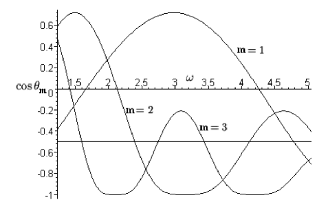
Figure 2: The restriction to Full Steiner Trees. The figure is a section $\alpha=\alpha_{R}$ (eq.(2.19)) of the surfaces given by eq.(2.16) corresponding to $m=1,2,3$.

The $m=1$ spanning tree is the only one which corresponds to Full Steiner trees in a large region of the $\omega$-interval convenient for our work. The other trees, $m=2,3$ correspond to forbidden regions in the same $\omega$-interval. The corresponding Steiner trees to be obtained from the positions of the points $S_{k+l_{S}m}$ and $P_{j+l_{P}m}$ are necessarily degenerate and should not be taken into consideration. Thus, the prescription (2.15) for the SRF function turns into

$$\rho(\omega,\alpha)=\frac{1+\alpha\omega\sqrt{\frac{A_{1}}{A_{1}+1}}}{\min_{(m)}\left(\sqrt{m^{2}\alpha^{2}\omega^{2}+A_{m}+1}\right)}=\mbox{Max}_{(m)}\,\,\rho_{m}(\omega,\alpha)$$ (2.17)

where

$$\rho_{m}(\omega,\alpha)=\frac{1+\alpha\omega\sqrt{\frac{A_{1}}{A_{1}+1}}}{\sqrt{m^{2}\alpha^{2}\omega^{2}+A_{m}+1}}.$$ (2.18)

The function (2.17) has a global minimum in the point

$$(\omega_{R},\alpha_{R})=\left(\pi-\arccos\frac{2}{3},\frac{\sqrt{30}}{9\left(\pi-\arccos\frac{2}{3}\right)}\right)$$ (2.19)

and

$$\rho(\omega_{R},\alpha_{R})=\frac{1}{10}(3\sqrt{3}+\sqrt{7})=0.78419037337\ldots$$ (2.20)

For a proof see [4].

The last value corresponds to the famous main conjecture of ref. [1] about the value of the Steiner Ratio in 3-dimensional Euclidean Space. It lead us also to think that Nature has solved the problem of energy minimization in the organization of intramolecular structure by choosing Steiner Trees as an intrinsic part of this structure [6].

3 The Stability of Steiner Trees Under Elastic Force Deformation

In the following we continue to work in a ${\mathbb{R}}^{3}$ manifold with an Euclidean distance definition. Let us now introduce a tree as that of figure (3)

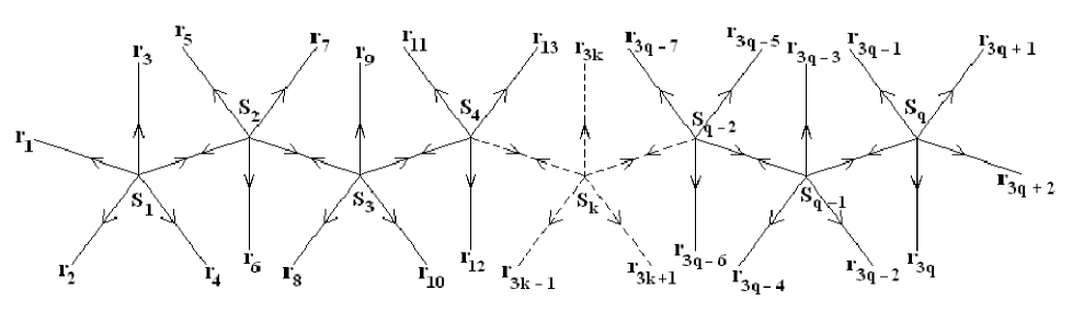
Figure 3: Geometrical scheme for a Steiner Problem with $p=5$.

There are $n$ input points (position vectors $\mathbf{r}_{j}$) and $q=(n-2)/(p-2)$ Steiner points (position vectors $\mathbf{S}_{k}$). If $q$ is not an integer number, there is not a tree with these $n$, $p$ values [7]. In figure (3) with $p=5$, we assume $n$ to be a feasible value. The knowledge of the Steiner Problem tell us that this tree structure is not stable since its total length can be reduced by decreasing the number $p$ [8]. The usual stable Steiner problem corresponds to $p=3$. In this section we shall give another proof of this fact by exploring the concept of a Steiner network with physical interaction among its vertices. The structure depicted at figure (3) is a representative of the network which models the fundamental interactions inside a biomacromolecule. Let us consider the interaction of this structure with similar structures. Let the resulting interaction forces as applied to input and Steiner points be $\mathbf{f}_{j}$, $\mathbf{f}_{S_{k}}$, respectively and let $l_{S_{k}r_{j}}$ be the length of an edge between a Steiner point and an input point on its neighbourhood. We have the following identities:

$$l_{S_{k}r_{j}}=\frac{1}{a_{j}}\,\mathbf{f}_{j}\,\,\cdot\,\,(\mathbf{r}_{j}-\mathbf{f}_{S_{k}})$$ (3.1)

$$l_{S_{k}S_{k+1}}=\frac{1}{a_{S_{k}}}\,\mathbf{f}_{S_{k}}\,\,.\,\,(\mathbf{S}_{k+1}-\mathbf{S}_{k})$$ (3.2)

where $a_{j}$, $a_{S_{k}}$, $j=1,2,\ldots,n$, $k=1,2,\ldots,q$ stand for the modulus of the parallel components to the edges of the resulting forces $\mathbf{f}_{j}$, $\mathbf{f}_{S_{k}}$, respectively.

The total length of the tree above is

$$l=\sum_{j=1}^{m-1}l_{S_{1}r_{j}}+\sum_{j=m}^{2m-3}l_{S_{2}r_{j}}+\sum_{j=2m-2}^{3m-5}\!\!\!l_{S_{3}r_{j}}+\ldots+\sum_{j=n-m+2}^{n}\!\!\!\!\!l_{S_{q}r_{j}}+\,\,\sum_{k=1}^{q-1}l_{S_{k}S_{k+1}}$$ (3.3)

From eqs.(2.20), (3.1), we can write the total length in the form

$$l = \sum_{j=1}^{n}\mathbf{r}_{j}\,\,\cdot\,\,\frac{\mathbf{f}_{j}}{a_{j}}-\mathbf{S}_{1}\cdot\left(\frac{\mathbf{f}_{S_{1}}}{a_{1}}+\sum_{j=1}^{p-1}\frac{\mathbf{f}_{j}}{a_{j}}\right)$$ (3.4)

$$- \sum_{k=2}^{q-1}\mathbf{S}_{k}\,\,\cdot\sum_{j=(k-1)p-2k+4}^{kp-2k+1}\left(\frac{\mathbf{f}_{j}}{a_{j}}+\frac{\mathbf{f}_{S_{k}}}{a_{S_{k}}}+\frac{(-\mathbf{f}_{S_{k-1}})}{a_{S_{k-1}}}\right)$$

$$- \mathbf{S}_{q}\,\,\cdot\,\left(\frac{(-\mathbf{f}_{S_{q-1}})}{a_{S_{q-1}}}+\sum_{j=n-p+2}^{n}\frac{\mathbf{f}_{j}}{a_{j}}\right)\,.$$

We now specialize this set of applied forces at the vertices as being collinear with the edges joining them, or

$$\mathbf{f}_{j}=a_{j}\hat{f}_{j||}\,\,;\,\,\,\,\,\,\,\,\,\,\,\,\,\,\mathbf{f}_{S_{k}}=a_{S_{k}}\hat{f}_{S_{k}||}$$ (3.5)

where the double vertical stroke means “collinear with the edge” and the hat over a letter stands as unit vector.

We now assume that the forces along the edges are Hooke elastic forces

$$\mathbf{f}_{j||}=C(\mathbf{r}_{j}-\mathbf{S}_{k})\,\,\,\,\,\,\,\,\,\mbox{or}\,\,\,\,\,\,\,\,\,\hat{f}_{j||}=\hat{r}_{j}=\frac{\mathbf{r}_{j}-\mathbf{S}_{k}}{||\mathbf{r}_{j}-\mathbf{S}_{k}||}$$ (3.6)

$$\mathbf{f}_{S_{k}||}=C(\mathbf{S}_{k+1}-\mathbf{S_{k}})\,\,\,\,\,\,\,\,\,\mbox{or}\,\,\,\,\,\,\,\,\,\hat{f}_{S_{k}||}=\hat{S}_{k}=\frac{\mathbf{S}_{k+1}-\mathbf{S}_{k}}{||\mathbf{S}_{k+1}-\mathbf{S}_{k}||}$$ (3.7)

where $C$ is the elastic constant.

The assumption of local equilibrium of these forces lead to the conditions:

$$\sum_{j=1}^{p-1}\hat{r}_{j}+\hat{S}_{1}=0$$ (3.8)

$$\sum_{j=(k-1)p-2k+4}^{kp-2k+1}\hat{r}_{j}+\hat{S}_{k}-\hat{S}_{k-1}=0,\,\,\,\,\,\,\,\,\,\,k=2,3,\ldots,q-1$$ (3.9)

$$\sum_{j=n-p+2}^{n}\hat{r}_{j}-\hat{S}_{q-1}=0\,.$$ (3.10)

This is a set of generalized Fermat problems or Steiner Problems [9].

For this equilibrium configuration, eq.(3.3) turns into

$$l=\sum_{j=1}^{n}\mathbf{r}_{j}\,\,\cdot\,\,\hat{f}_{j||}\,.$$ (3.11)

The stability of this equilibrium configuration under a variation of the applied forces can be tested by

$$\delta l=\sum_{j=1}^{n}\mathbf{r}_{j}\,\,\cdot\,\,\delta\hat{f}_{j||}=0\,.$$ (3.12)

We take cartesian coordinates for the ${\mathbb{R}}^{3}$ vectors $\mathbf{r}_{j}=(x_{i},y_{i},z_{i})$, $\mathbf{S}_{k}=(x_{S_{k}},y_{S_{k}},z_{S_{k}})$ and we consider the three independent variations $\delta_{x_{S_{k}}}$, $\delta_{y_{S_{k}}}$, $\delta_{z_{S_{k}}}$ in the coordinates of the Steiner points.

The corresponding variations in the length of the tree are of the form

$$\delta_{x_{S_{k}}}l=\delta_{x_{S_{k}}}\cdot\sum_{j=1}^{n}\frac{-x_{j}(\mathbf{r}_{j}-\mathbf{S}_{k})^{2}+[(\mathbf{r}_{j}-\mathbf{S}_{k})\cdot\mathbf{r}_{j}](x_{j}-x_{S_{k}})}{||\mathbf{r}_{j}-\mathbf{S}_{k}||^{3}}=0$$ (3.13)

and two other analogous expressions for the variations $\delta_{y_{S_{k}}}$, $\delta_{z_{S_{k}}}$.

From the arbitrariness of these variations we can write,

$$\sum_{j=1}^{n}\frac{(\mathbf{r}_{j}-\mathbf{S}_{k})\times[(\mathbf{r}_{j}-\mathbf{S}_{k})\times\mathbf{r}_{j}]}{||\mathbf{r}_{j}-\mathbf{S}_{k}||^{3}}=0\,.$$ (3.14)

We can also write

$$\sum_{j=1}^{n}\frac{(\mathbf{r}_{j}\,\,\cdot\,\,\mathbf{S}_{k})^{2}-r_{j}^{2}S_{k}^{2}}{||\mathbf{r}_{j}-\mathbf{S}_{k}||^{3}}=0\,.$$ (3.15)

We now write the position vectors $\mathbf{r}_{j}$, $\mathbf{S}_{k}$ for the configuration depicted at figure (3). The points can be taken as evenly spaced along right circular helices which radii are 1 and $R_{p}$, respectively. We have,

$$\mathbf{r}_{j}=(\cos(j-1)\omega,\sin(j-1)\omega,\alpha(j-1)\omega)$$ (3.16)

$$\mathbf{S}_{k}=(R_{p}\cos k\omega,R_{p}\sin k\omega,\alpha k\omega)\,.$$ (3.17)

$R_{p}(\omega,\alpha)$ is a function which can be derived from the equilibrium conditions in eqs.(3.7)–(3.9). For $p=3$ there is only one solution given by

$$R_{3}(\omega,\alpha)=\frac{\alpha\omega}{\sqrt{A_{1}(A_{1}+1)}}\,\,;\,\,\,\,\,\,A_{1}=1-2\cos\omega\,.$$ (3.18)

This solution coincides with eq.(1.3).

For $p>3$, another useful solution could be obtained from the equations:

$$\cos(\hat{r}_{j},\hat{r}_{l})=\cos(\hat{r}_{j},\hat{S}_{k})=\cos(\hat{S}_{k},\hat{S}_{m})=-\frac{1}{(p-1)}$$

$$\hskip 85.35826ptj,l=1,2,\cdots,n;\,\,\,\,k,m=1,2,\cdots,q.$$

Curiously, Nature has chosen this solution for $p=4$ to keep sure of partial equilibrium of side chains between the Amide plane conformation in proteins [6, 10, 11].

For the configuration given by eqs.(3.15)–(3.16), eq.(3.15) can be written as

$$\sum_{j=1}^{n}T_{jkp}(\omega,\alpha)=0$$

where the geometrical object $T_{jkp}$ can be written in the coordinates of eqs.(3.16) and (3.17) as

$$T_{jkp}=\hskip 335.7426pt$$

$$\frac{[\cos^{2}(j\!\!-\!\!1\!\!-\!\!k)\omega\!\!-\!\!1\!\!-\!\!\alpha^{2}\omega^{2}(j\!\!-\!\!1)^{2}]R_{p}^{2}+\alpha^{2}\omega^{2}[2R_{p}(j\!\!-\!\!1)k\cos(j\!\!-\!\!1\!\!-\!\!k)\omega\!\!-\!\!k^{2}]}{[1+R_{p}^{2}\!\!-\!\!2R_{p}\cos(j\!\!-\!\!1\!\!-\!\!k)\omega+\alpha^{2}\omega^{2}(j\!\!-\!\!1\!\!-\!\!k)^{2}]^{3/2}}.$$

(3.19)

To each $k$-value, there will be a term $j=k+1$ which dominates the sum above. However, we cannot have $j=k+1$ for $p>3$. This can be seen from the fact for a vertex $S_{k}$ ($k\neq 1,q$) there are ($p-2$) nearest external vertices $r_{j}$. The sequence of their consecutive position vectors is

$$\mathbf{r}_{(k-1)p-2k+4},\ldots\ldots,\mathbf{r}_{kp-2k+1}$$ (3.20)

and the requirement $j=k+1$ corresponds to an integer $p$-value only for $p=3$.

This $p=3$ case which is known to correspond to the most stable problem [8] has as a possible configuration the figure (4) below

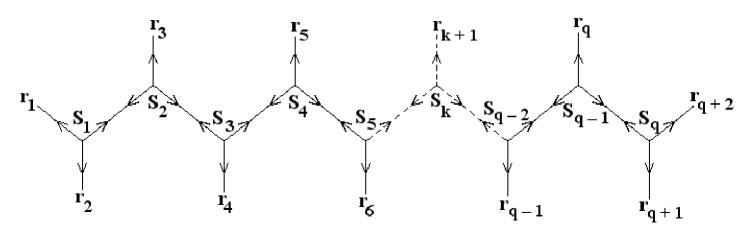
Figure 4: The stable structure of the $p=3$ Steiner Problem.

4 Concluding Remarks

We have stressed on some past publications that there is a self-consistent treatment of the intramolecular organization of biomacromolecules in terms of Steiner networks. This representation is able at deriving information concerning its stability and evolution. The supporting facts for stability are now well-established and the ideas related to the evolution of macromolecules are in their way to be developed and accepted as a preliminary theory of molecular evolution. The missing subject is a full description of geometric chirality and in order to unveil some of its properties, we have proposed to study the influence of some proposals for chirality measure on the dynamics of optimization problems. These are aimed at studying the structures which energy is around the assumed energy of the minimum solution and the variation process of the chiral properties in the neighbourhood of this minimum. We think that this research line is worth of serious scientific work and should take advantage of the best efforts of very good scientific researchers for some years.

References

- [1] Smith, W.D. and MacGregor Smith, J.: On the Steiner Ratio in 3-Space. J. Comb. Theor. A69, 301–332 (1995).
- [2] Mondaini, R.P.: The Euclidean Steiner Ratio and the Measure of Chirality of Biomacromolecules. Gen. Mol. Biol. 27(4), 658–664 (2004).
- [3] Mondaini, R.P.: The Steiner Ratio and the Homochirality of Biomacromolecular Structures. Nonconvex Optimization and its Applications Series – Kluwer Acad. Publ. 74, 373–390 (2004).
- [4] Mondaini, R.P., Oliveira, N.V.: A New Approach to the Study of the Smith + Smith Conjecture. http://www.arxiv.org/math-ph/0506050 (2005).
- [5] Mondaini, R.P.: Modelling the Biomacromolecular Structure with Selected Combinatorial Optimization Techniques. http://www.arxiv.org/math-ph/0502051 (2005).
- [6] MacGregor Smith, J., Toppur, B.: Euclidean Steiner Minimal Trees, Minimal Energy Configurations, and the Embedding Problem of Weighted Graphs in . Discret. Appl. Math. 71, 187–215 (1996).
- [7] Mondaini, R.P.: The Disproof of a Conjecture on the Steiner Ratio in and its consequences for a Full Geometric Description of Macromolecular Chirality. Proc. BIOMAT Symp. 2, 101–177 (2003).
- [8] Gilbert, E. N. and Pollak, H. O.: Steiner Minimal Trees. SIAM J. Appl. Math. 16, 1 (1968).
- [9] Kuhn, H. W.: Steiner’s problem revisited. In: Studies in Optimization, Studies in Math. G.B. Dantzig, B. C. Eaves (eds.) 10 Math. Assoc. Amer. 53–70 (1975).
- [10] Voet, D., Voet, J.G.: Biochemistry. 2nd ed., Wiley, New York (1995).
- [11] Glusker, J.P., Lewis, M., Rossi, M.: Crystal Structure Analysis for Chemists and Biologists. VHC Publications Inc. (1994).