Transverse Evolution Operator for the Gross–Pitaevskii Equation

Transverse Evolution Operator
for the Gross–Pitaevskii Equation
in Semiclassical Approximation

Alexey BORISOV ^†, Alexander SHAPOVALOV ^†‡§ and Andrey TRIFONOV ^‡§

A. Borisov, A. Shapovalov and A. Trifonov

^† Tomsk State University, 36 Lenin Ave., 634050 Tomsk, Russia borisov@phys.tsu.ru, shpv@phys.tsu.ru

^‡ Tomsk Polytechnic University, 30 Lenin Ave., 634050 Tomsk, Russia trifonov@mph.phtd.tpu.edu.ru

^§ Math. Phys. Laboratory, Tomsk Polytechnic University, 30 Lenin Ave., 634050 Tomsk, Russia

Received July 27, 2005, in final form November 13, 2005; Published online November 22, 2005

The Gross–Pitaevskii equation with a local cubic nonlinearity that describes a many-dimensional system in an external field is considered in the framework of the complex WKB–Maslov method. Analytic asymptotic solutions are constructed in semiclassical approximation in a small parameter $\hbar$, $\hbar\to 0$, in the class of functions concentrated in the neighborhood of an unclosed surface associated with the phase curve that describes the evolution of surface vertex. The functions of this class are of the one-soliton form along the direction of the surface normal. The general constructions are illustrated by examples.

WKB–Maslov complex germ method; semiclassical asymptotics; Gross–Pitaevskii equation; solitons; symmetry operators

81Q20; 81R30; 35Q55

1 Introduction

The Gross–Pitaevskii equation (GPE), derived independently by Gross [1] and Pitaevskii [2], arises in various models of nonlinear physical phenomena. This is a Schrödinger-type equation with an external field potential $U(\vec{x},t)$ and a local cubic nonlinearity:

$$\left(-i\hbar\partial_{t}+\frac{{\widehat{\vec{p}}}\,^{2}}{2m}+U(\vec{r})+\varkappa|\Psi(\vec{x},t,\hbar)|^{2}\right)\Psi(\vec{x},t,\hbar)=0.$$ (1)

Here $\vec{x}=(x_{j})\in\mathbb{R}^{n}$; $i,j,k,l=1,\ldots,n$; $t\in\mathbb{R}^{1}$; $\partial_{t}=\partial/\partial t$; $\widehat{\vec{p}}=-i\hbar\nabla$; $\nabla$ is a gradient operator in $\vec{x}$; $\varkappa$ and $\hbar$ are real parameters. The complex function $\Psi(\vec{x},t,\hbar)$ determines the system state, $|\Psi|^{2}=|\Psi(\vec{x},t,\hbar)|^{2}=\Psi(\vec{x},t,\hbar)\Psi^{*}(\vec{x},t,\hbar)$; the function $\Psi^{*}(\vec{x},t,\hbar)$ is complex conjugate to $\Psi(\vec{x},t,\hbar)$.

For $U=0$, $\varkappa<0$, and $n=1$, equation (1) is known to be integrable by the Inverse Scattering Transform (IST) method [3, 4] and to have exact soliton solutions. The solutions are written in terms of space localized functions which conserve their form during the evolution. Solitons have numerous physical applications; for example, they serve to describe the propagation of optical pulse in nonlinear media [5, 6].

The solutions of equation (1) that are not completely localized are also of interest, in particular, in the theory of nonlinear deep-water waves where the two-dimensional ($n=2$) solutions of plane wave solitonlike type are localized only along the wave propagation direction [7].

The Gross–Pitaevskii equation (1) in physical dimensions ($n=2,3$) is used in the mean-field quantum theory of Bose-Einstein condensate (BEC) formed by ultracold bosonic coherent atomic ensembles [8]. As a rule, the function $U(\vec{x},t)$ is the potential of an external field of a magnetic trap and laser radiation. The wave function $\Psi(\vec{x},t,\hbar)$ corresponds to a condensate state. The local nonlinearity term $\varkappa|\Psi(\vec{x},t,\hbar)|^{2}$ arises from an assumption about the delta-shape interatomic potential. For multidimensional cases, no method of exact integration of the GPE is known, to our knowledge, and equation (1) is usually studied for some special cases by computer simulation. However, this approach has natural restrictions and also has nontrivial specific features as long as localized solutions of equation (1) are known to be unstable and to collapse when $n>1$, $U=0$, and $\varkappa<0$ [9]. Therefore, to develop methods for constructing analytical solutions of the GPE (1) for many-dimensional cases is critical.

In this paper we construct a class of asymptotic solutions for the $(1+n)$-dimensional GPE with a focusing local cubic nonlinearity

$$\widehat{L}(\Psi)(\vec{x})=\left[-i\hbar\partial_{t}+{\mathcal{H}}(\hat{\vec{p}},\vec{x},t)-g^{2}|\Psi(\vec{x},t,\hbar)|^{2}\right]\Psi(\vec{x},t,\hbar)=0.$$ (2)

Here $g$ is a real nonlinearity parameter and $\hbar$ is an asymptotic parameter, $\hbar\to 0$. The pseudo-differential operator ${\mathcal{H}}(\hat{\vec{p}},\vec{x},t)$ is Weyl-ordered [10] and its symbol ${\mathcal{H}}({\vec{p}},\vec{x},t)$ is quadratic in $\vec{p}\in\mathbb{R}^{n}$

$${\mathcal{H}}(\hat{\vec{p}},\vec{x},t)=\frac{1}{2}\langle\hat{\vec{p}},{\mathcal{H}}_{pp}(t)\hat{\vec{p}}\rangle+\frac{1}{2}\left(\langle\hat{\vec{p}},\vec{\mathcal{H}}(\vec{x},t)\rangle+\langle\vec{\mathcal{H}}(\vec{x},t),\hat{\vec{p}}\rangle\right)+{\mathcal{H}}_{0}(\vec{x},t),$$ (3)

where $\langle\vec{a},\vec{b}\rangle=$ $\sum\limits_{l=1}^{n}a_{l}b_{l}$; the real functions — the $(n\times n)$-matrix ${\mathcal{H}}_{pp}(t)$, the vector $\vec{\mathcal{H}}(\vec{x},t)$, and the scalar ${\mathcal{H}}_{0}(\vec{x},t)$ — smoothly depend on their arguments. These functions model the external fields imposed on the system described by equation (2).

A formalism of semiclassical asymptotics was developed for the GPE with a nonlocal nonlinearity in [11, 12]. This equation was named the Hartree type equation. The semiclassical asymptotics of the nonstationary Hartree type equation were also studied [13, 14, 15, 16, 17, 18, 19, 20]. This formalism is based on the WKB-Maslov complex germ method, the idea of which was first put forward in [21] and then comprehensively treated in [22, 23, 24].

Further developments of the Maslov method [25, 26] (see also [27] and references therein) allow one to construct the localized solutions of the Cauchy problem in the class of trajectory – concentrated functions.

Here we apply the ideas of the complex germ method and the approach used in [11, 12] to construct the analytic solutions asymptotic in a small parameter $\hbar$, $\hbar\to 0$, for equation (2). The asymptotic solutions are constructed in the class of functions localized in the vicinity of an unclosed surface associated with the phase curve that describes the evolution of the surface vertex.

The functions of this class have the one-soliton form of the one-dimensional nonlinear Schrödinger equation along the surface normal direction. A semiclassical linearization of equation (2) is performed accurate to $O(\hbar^{3/2})$, $\hbar\to 0$. The asymptotic solutions constructed are illustrated by examples.

2 The class of paraboloid-concentrated solitonlike functions

Let us describe a class of functions $\Psi(\vec{x},t,\hbar)$ in which the asymptotics for the GPE (2) are constructed. Following [11, 12], consider equation (2) for the $(1+1)$-dimensional case with no external field ($U=0$)

$$\left(i\hbar\partial_{t}+\frac{1}{2}\hbar^{2}\partial_{x}^{2}+g^{2}|\Psi(x,t,\hbar)|^{2}\right)\Psi(x,t,\hbar)=0,$$ (4)

where $x\in\mathbb{R}^{1}$ and $\partial_{x}=\partial/\partial x$. Equation (4) has a one-soliton solution [3, 4]

$$\Psi(x,t,\hbar)=-\frac{2\eta}{g}\,\frac{1}{{\rm ch}[2\eta(x-x_{0}-{2\xi}t)/{\hbar}]}\exp\left[\frac{i}{\hbar}\big{(}2\xi x-{2}\big{(}\xi^{2}-\eta^{2}\big{)}t+\varphi_{0}\big{)}\right],$$ (5)

where $\xi$, $\eta$, $x_{0}$, and $\varphi_{0}$ are the real parameters.

Earlier [28] we obtained a semiclassical solution of equation (2) with the leading term

$$\Psi(\vec{x},t,\hbar)=g^{-1}\sqrt{\langle\nabla\sigma,{\mathcal{H}}_{pp}(t)\nabla\sigma\rangle}\exp\left(\frac{i}{\hbar}S(\vec{x},t,\hbar)\right){\rm ch^{-1}}\left(\frac{1}{\hbar}\sigma(\vec{x},t,\hbar)\right).$$ (6)

It was assumed that the complex function $\Omega(\vec{x},t,\hbar)=S(\vec{x},t,\hbar)+i\sigma(\vec{x},t,\hbar)$ regularly depends on $\hbar$ and its high-order part, i.e., the function $\Omega(\vec{x},t,0)=$ $\Omega^{(0)}(\vec{x},t)=$ $S^{(0)}(\vec{x},t)+i\sigma^{(0)}(\vec{x},t)$, is a complex solution of the Hamilton–Jacobi equation

$$\partial_{t}\Omega^{(0)}+\mathcal{H}\big{(}\nabla{\Omega^{(0)}},\vec{x},t\big{)}=0.$$ (7)

The functions (6) are localized in the neighborhood of a $t$-parameter family of surfaces

$$\Gamma^{t}=\big{\{}\vec{x}:\sigma(\vec{x},t,0)=\sigma^{(0)}(\vec{x},t)=0\big{\}}.$$ (8)

Assume that the rank of Hesse matrix of the function $\sigma^{(0)}(\vec{x},t)$ is $n$ at any point $\vec{x}\in\Gamma^{t}$.

The construction of global solutions of equation (7) is beyond the scope of this work. Here we consider the evolution of the functions localized in the neighborhood $U_{\vec{x}_{0}}$ of the surface point $\vec{x}_{0}$ (8) at the initial time $t=0$.

Denote by

$$\gamma=\big{\{}\vec{x}:\vec{x}\in\mathbb{R}^{n},\vec{x}=\vec{X}(t),t\geqslant 0\big{\}}$$

a smooth curve passing through the point $\vec{x}_{0}$ ($=\vec{X}(0)$) in the coordinate space $\vec{x}\in\mathbb{R}^{n}$ such that $\vec{X}(t)\in\Gamma^{t}$. This curve plays the role of the “classical trajectory” corresponding to the solution of the quantum equation (2).

In the neighborhood $\tilde{U}_{\vec{X}(t)}\subset\Gamma^{t}$ of the point $\vec{X}(t)\in\gamma$, the hypersurface $\Gamma^{t}$ can be approximated by a simpler surface, for example, by the tangent plane. It is well known that a tangent plane is determined uniquely by its normal and the point of contact. Let $\vec{\pi}(t)$ be a normal vector to the surface $\Gamma^{t}$ at a point $\vec{x}=\vec{X}(t)$.

To construct asymptotic solutions of equation (2) one needs the complex germ [22], i.e. the $n$-dimensional complex space associated with the equation under consideration and functions defined in the neighborhood of the hypersurface (8).

It is more precise to use a second order surface

$$\langle\vec{\pi}(t),\Delta\vec{x}\rangle+\frac{1}{2}\langle\Delta\vec{x},Q_{2}(t)\Delta\vec{x}\rangle=0,\qquad\Delta\vec{x}=\vec{x}-\vec{X}(t),$$ (9)

instead of the tangent plane. The surface (9) with a proper choice of the matrix $Q_{2}(t)$ is a quadratic approximation of (8) in the neighborhood $\tilde{U}_{\vec{X}(t)}$.

Introduce the class ${\mathcal{N}}^{t}_{\hbar}$ of complex functions with the generic element

$$\Psi(\vec{x},t,\hbar)=\Phi(\theta,\vec{x},t,\hbar)=g^{-1}\sqrt{\langle\vec{\pi}(t),\mathcal{H}_{pp}(t)\vec{\pi}(t)\rangle}\exp\left(\frac{i}{\hbar}S(\vec{x},t,\hbar)\right)$$

$$\phantom{\Psi(\vec{x},t,\hbar)=}{}\times{\rm ch}^{-1}(\theta)\big{\{}1+\hbar\,{\rm ch}(\theta)u(\theta,\vec{x},t,\hbar)+i\hbar\,{\rm ch}(\theta)v(\theta,\vec{x},t,\hbar)\big{\}}.$$ (10)

The functions (10) are localized in the neighborhood $U_{\vec{X}(t)}$ of the point $\vec{x}=\vec{X}(t)$. This point is the “vertex” of the surface (9). In equation (10), $\theta=\sigma(\vec{x},t,\hbar)/{\hbar}$ is a “fast” variable; the real functions $u=u(\theta,\vec{x},t,\hbar)$ and $v=v(\theta,\vec{x},t,\hbar)$ are regular in their arguments and are bounded in $\theta$, and

$$\sigma(\vec{x},t,\hbar)=\langle\vec{\pi}(t),\Delta\vec{x}\rangle+\frac{1}{2}\langle\Delta\vec{x},Q_{2}(t)\Delta\vec{x}\rangle+\hbar\sigma^{1}(\vec{x},t,\hbar),$$ (11)

$$S(\vec{x},t,\hbar)=S^{0}(t)+\langle\vec{P}(t),\Delta\vec{x}\rangle+\frac{1}{2}\langle\Delta\vec{x},Q_{1}(t)\,\Delta\vec{x}\rangle+\hbar S^{1}(\vec{x},t,\hbar).$$ (12)

In equations (11) and (12), the real function $S^{0}(t)$, the real $n$-dimensional vector functions $\vec{\pi}(t)$, $\vec{P}(t)$, and $\vec{X}(t)$, the real $(n\times n)$-matrix functions $Q_{1}(t)$ and $Q_{2}(t)$, the real functions $\sigma^{1}(\vec{x},t,\hbar)=\tilde{\sigma}^{1}(\vec{\xi},t,\hbar)$ and $S^{1}(\vec{x},t,\hbar)=\tilde{S}^{1}(\vec{\xi},t,\hbar)$, $\vec{\xi}={\vec{\Delta}x}/{\sqrt{\hbar}}$ are functional parameters of the class ${\mathcal{N}}^{t}_{\hbar}$; $\Delta\vec{x}=\vec{x}-\vec{X}(t)$.

Note that in constructing the class ${\mathcal{N}}^{t}_{\hbar}$, a specific basis, “orthogonal” in some way to the vector $\vec{\pi}(t)$, is used. As a result, the classical trajectory depends on the complex germ as well.

The functions (10) are not normalizable in the space $L_{2}({\mathbb{R}}^{n},d\vec{x})$ since they are localized on an unclosed surface, equation (9). Therefore, the surface $\Gamma^{t}$ (8) (compact in some physical applications) is substituted by its quadratic approximation (9) in the neighborhood $U_{\vec{X}(t)}$. As we are interested in finding functions localized in $U_{\vec{X}(t)}$, we come to the problem of small perturbations on the “background” of the hypersurface (9). To eliminate the “background”, consider the function

$$\tilde{\Psi}(\vec{x},t,\hbar)=\Phi(\theta,\vec{x},t,\hbar)-\Phi(\theta_{0},\vec{x},t,\hbar)\thickapprox g^{-1}\frac{d}{d\theta}\sqrt{{\langle\vec{\pi},{\mathcal{H}}_{pp}(t)\vec{\pi}\rangle}}\,{\rm ch}^{-1}(\theta)$$

$$\phantom{\tilde{\Psi}(\vec{x},t,\hbar)=}{}\times\exp\left(\frac{i}{\hbar}S(\vec{x},t,\hbar)\right)\left\{1+\hbar\,{\rm ch}(\theta)u(\theta,\vec{x},t,\hbar)+i\hbar\,{\rm ch}(\theta)v(\theta,\vec{x},t,\hbar)\right\}\Bigg{|}_{\theta=\theta_{0}}\!\!\theta_{1},\!\!\!$$ (13)

$$\theta=\theta_{0}+\theta_{1},\qquad\theta_{0}=\frac{1}{\hbar}\langle\vec{\pi}(t),\Delta\vec{x}\rangle+\frac{1}{2\hbar}\langle\Delta\vec{x},Q_{2}(t)\Delta\vec{x}\rangle,\qquad\theta_{1}=\tilde{\sigma}^{1}(\vec{\xi},t,\hbar).$$

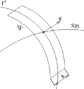
Figure 1:

The functions $\tilde{\Psi}(\vec{x},t,\hbar)$, equation (13), are normalizable in $L_{2}({\mathbb{R}}^{n},d\vec{x})$. Estimating the solutions of equation (2), we use the norm of the functions $\tilde{\Psi}(\vec{x},t,\hbar)$. Taking into account this normalization condition, let us assume that the functions $\tilde{\sigma}^{1}(\vec{\xi},t,\hbar)$ and $\tilde{S}^{1}(\vec{\xi},t,\hbar)$ belong to the Schwartz space ${\mathcal{S}}({\mathbb{R}}^{n-1}_{\xi},d\mu)$, where $d\mu$ is the measure on the hypersurface, determined by equation (9).

The class ${\mathcal{N}}^{t}_{\hbar}$ of the form (10) with $n=1$ includes the exact one-soliton solution (5) of one-dimensional nonlinear Schrödinger equation (4) with a special choice of the functional parameters of the class. If the rank of matrix $Q_{2}(t)$ is $n$, then in one-dimensional case equation (10) can not be transformed to (5) since the argument $\theta$ of the hyperbolic cosine contains the terms quadratic in $x$. The sufficient conditions for such a transformation are

$${\rm rank}\,(Q_{2}(t))=n-1,\qquad{\rm rank}\,(Q_{2}(t),\vec{\pi}(t))=n,$$ (14)

where $(Q_{2}(t),\vec{\pi}(t))$ is the augmented matrix of order $n\times(n+1)$. Note that under conditions (14), the surface (9) has the paraboloidal shape.

Let us expand the operator $\widehat{L}$ in equation (2) in the neighborhood $U_{\vec{X}(t)}$ under the conditions

$$\Delta x_{k}=\hat{O}\big{(}\hbar^{1/2}\big{)},\qquad\Delta\hat{p}_{k}\Big{|}_{\theta=\mathop{\rm const}}=\hat{O}\big{(}\hbar^{1/2}\big{)},\qquad\langle\vec{\pi}(t),\Delta\vec{x}\rangle=\hat{O}(\hbar).$$ (15)

The leading term of the asymptotic in the class of functions (10) under conditions (15) has the form (6).

It is determined by the phase curve $z=Z(t,\hbar)=(\vec{P}(t,\hbar),\vec{X}(t,\hbar))$, vector $\vec{\pi}=\vec{\pi}(t)$, and functions $\sigma(\vec{x},t,\hbar)$ and $S(\vec{x},t,\hbar)$ of the form (11) and (12), respectively. We call these functions the paraboloid-concentrated solitonlike functions.

3 The linear associated Schrödinger equation

The asymptotic leading term is obtained when the asymptotic solution of the equation (2) is constructed accurate to $O(\hbar^{2})$ [28].

Let us substitute (10) in (2), take into account the terms of order $O(\hbar^{2})$, separate the equations with respect to the “fast” variable, and find the solutions of these equations that decrease as $\theta\to\pm\infty$. We than obtain for the function $\Omega=S+i\sigma$

$$\Omega_{t}+{\mathcal{H}}(\nabla\Omega,\vec{x},t)-\frac{i\hbar}{2}\bigg{[}\mathop{\rm Sp}[{\mathcal{H}}_{pp}(t)\Omega_{xx}+{\mathcal{H}}_{px}(\nabla\Omega,\vec{x},t)]$$

$$\phantom{\Omega_{t}}{}+{\langle\vec{\pi},{\mathcal{H}}_{pp}(t)\vec{\pi}\rangle}^{-1}\frac{d}{dt}\langle\vec{\pi},{\mathcal{H}}_{pp}(t)\vec{\pi}\rangle\bigg{]}=0.$$ (16)

With the substitution $\Omega=-i\hbar\ln\left[{\psi(\vec{x},t,\hbar)}{{\langle\vec{\pi},{\mathcal{H}}_{pp}(t)\vec{\pi}\rangle}^{-1/2}}\right]$, equation (16) yields

$$\big{[}-i\hbar\partial_{t}+{\mathcal{H}}(\hat{\vec{p}},\vec{x},t)\big{]}\psi(\vec{x},t,\hbar)=O\big{(}\hbar^{3/2}\big{)},$$

where the operator ${\mathcal{H}}(\hat{\vec{p}},\vec{x},t)$ has the form of (3),

$$\psi(\vec{x},t,\hbar)=\sqrt{\langle\vec{\pi},\mathcal{H}_{pp}(t)\vec{\pi}\rangle}\exp\left[{\frac{i}{\hbar}\Omega(\vec{x},t,\hbar)}\right]=\exp\left[\frac{i}{\hbar}S(\vec{x},t,\hbar)\right]\varphi(\vec{x},t,\hbar),$$ (17)

$$\varphi(\vec{x},t,\hbar)=\sqrt{\langle\vec{\pi},{\mathcal{H}}_{pp}(t)\vec{\pi}\rangle}\exp\left[{-\frac{1}{\hbar}\sigma(\vec{x},t,\hbar)}\right].$$

We call the equation

$$\big{[}-i\hbar\partial_{t}+{\mathcal{H}}(\hat{\vec{p}},\vec{x},t)\big{]}\psi(\vec{x},t,\hbar)=0$$ (18)

the linear associated Schrödinger equation corresponding to the GPE (2).

Therefore, the leading term of the asymptotic solution of the nonlinear equation (2) is constructed by using a solution of the linear equation (18) with conditions (6) and (17).

Note that for the function (6) to satisfy (14) the solution (17) must be chosen in a specific way. Denote the class of these functions by ${\mathcal{S}}_{\hbar}^{t}$.

Let us seek the solutions to equation (18) that possess this property in the class of functions

$$\psi(\vec{x},t,\hbar)=\exp\left[-\frac{1}{\hbar}\langle\vec{\pi},\Delta\vec{x}\rangle\right]\phi(\vec{x},t,\hbar).$$ (19)

Substitution of (19) in (18) yields

$$\big{[}-i\hbar\partial_{t}+i\langle\dot{\vec{\pi}},\Delta\vec{x}\rangle-i\langle{\vec{\pi}},\dot{\vec{x}}\rangle+{\mathcal{H}}\big{(}\vec{p}(t)+i\vec{\pi}+\Delta\hat{\vec{p}},\vec{x},t\big{)}\big{]}\phi(\vec{x},t,\hbar)=O\big{(}\hbar^{3/2}\big{)}.$$ (20)

Let us expand the operator of equation (20) in a power series in $\Delta\vec{x}$ accurate to $O\big{(}\hbar^{3/2}\big{)}$ in terms of the accuracy of (15). We then have

$$\Big{[}-i\hbar\partial_{t}-i\big{[}\langle{\vec{\pi}},(\dot{\vec{x}}-{\mathcal{H}}_{\vec{p}}(t))\rangle-\langle(\dot{\vec{\pi}}+{\mathcal{H}}_{xp}(t)\vec{\pi}),\Delta\vec{x}\rangle-\langle{\vec{\pi},{\mathcal{H}}_{pp}(t)\Delta\hat{\vec{p}}}\rangle\big{]}$$

$$\qquad{}+{\mathcal{H}}(t)-\frac{1}{2}\langle{\vec{\pi},{\mathcal{H}}_{pp}(t)\vec{\pi}}\rangle+\langle{{\mathcal{H}}_{\vec{x}}(t),\Delta\vec{x}}\rangle+\langle{{\mathcal{H}}_{\vec{p}}(t),\Delta\hat{\vec{p}}}\rangle$$

$$\qquad{}+\frac{1}{2}\Big{[}\langle{\Delta\vec{x},{\mathcal{H}}_{xx}(t)\Delta\vec{x}}\rangle+\langle{\Delta\vec{x},{\mathcal{H}}_{xp}(t)\Delta\hat{\vec{p}}}\rangle+\langle{\Delta\hat{\vec{p}},{\mathcal{H}}_{px}(t)\Delta\vec{x}}\rangle$$

$$\qquad{}+\langle{\Delta\hat{\vec{p}},{\mathcal{H}}_{pp}(t)\Delta\hat{\vec{p}}}\rangle\big{]}\Big{]}\phi+O\big{(}\hbar^{3/2}\big{)}=\big{[}-i\hbar\partial_{t}+\hat{\mathcal{H}}_{0}(t)\big{]}\phi+O\big{(}\hbar^{3/2}\big{)}=0.$$ (21)

Therefore, for the solution (19) in the approximation under consideration, the linear associated Schrödinger equation (18) takes the form

$$\big{[}-i\hbar\partial_{t}+\hat{\mathcal{H}}_{0}(t)\big{]}\phi=0.$$ (22)

Here the operator $\hat{\mathcal{H}}_{0}(t)$ (quadratic with respect to the operators $\Delta{\vec{x}}$ and $\Delta\hat{\vec{p}}\,$) is obtained from (21).

Thus, the construction of asymptotic leading term (6) in the class of functions (19) for the nonlinear equation (2) by solving equation (22) is complete.

4 Solutions of the Gross–Pitaevskii equation

The solutions of equation (22) are well-known (see, e.g., [29, 30, 31]). In particular, the evolution operator $\hat{U}_{{\mathcal{H}}_{0}}(t,s)$ is found in explicit form, whose action on the function $\psi(\vec{x},\hbar)$ referred to a time $t=s$ is given by the relation

$$\psi(\vec{x},t,\hbar)=\hat{U}_{{\mathcal{H}}_{0}}(t,s)\psi(\vec{x},\hbar)=\int_{{\mathbb{R}}^{n}}G_{{\mathcal{H}}_{0}}(\vec{x},\vec{y},t,s)\psi(\vec{y},\hbar)d\vec{y}.$$ (23)

Here $G_{{\mathcal{H}}_{0}}(\vec{x},\vec{y},t,s)$ is the Green function of the linear associated Schrödinger equation (22), which is determined by the following conditions:

$$\big{\{}-i\hbar\partial_{t}+\hat{\mathcal{H}}_{0}(t)\big{\}}G_{{\mathcal{H}}_{0}}(\vec{x},\vec{y},t,s)=0,\qquad\lim_{t\to s}G_{{\mathcal{H}}_{0}}(\vec{x},\vec{y},t,s)=\delta(\vec{x}-\vec{y}).$$ (24)

To construct a subclass of the class ${\mathcal{N}}^{t}_{\hbar}$ (10) of solutions of equation (2), let us find a particular solution in the form

$$\phi(\vec{x},t)=N_{\phi}\exp\left\{\frac{i}{\hbar}\left[S^{0}(t)+\hbar S^{1}(t)+i\hbar\sigma^{1}(t)+\langle\vec{P}(t),\Delta\vec{x}\rangle+\frac{1}{2}\langle\Delta\vec{x},Q(t)\Delta\vec{x}\rangle\right]\right\},$$ (25)

where the functions $S^{0}(t)$, $S^{1}(t)$, and $\sigma^{1}(t)$, the $n$-dimensional vectors $\vec{P}(t)$, $\vec{X}(t)$, and the complex $(n\times n)$-matrix $Q(t)$=$Q_{1}(t)+iQ_{2}(t)$ are to be determined; $N_{\phi}$ is a constant.

Substituting (25) in (21) and setting $\dot{\vec{X}}={\mathcal{H}}_{\vec{p}}$, $Q(t)=Q_{1}(t)+iQ_{2}(t)$, we obtain the determining system of equations for $\vec{P}(t)$, $\vec{\pi}(t)$, $\vec{X}(t)$, $Q(t)$

$$\dot{\vec{P}}=-{\mathcal{H}}_{\vec{x}}(\vec{P},\vec{X},t)+Q_{2}{\mathcal{H}}_{pp}(t)\vec{\pi},$$ (26)

$$\dot{\vec{X}}={\mathcal{H}}_{\vec{p}}(\vec{P},\vec{X},t),$$

$$\dot{\vec{\pi}}=-\big{[}{\mathcal{H}}_{xp}\big{(}\vec{P},\vec{X},t\big{)}+Q_{1}(t){\mathcal{H}}_{pp}(t)\big{]}\vec{\pi},$$

$$\dot{Q}+{\mathcal{H}}_{xx}(t)+{\mathcal{H}}_{xp}(t)Q+Q{\mathcal{H}}_{px}(t)+Q{\mathcal{H}}_{pp}(t)Q=0.$$ (27)

Consider the following system of equations

$$\dot{\vec{Z}}={\mathcal{H}}_{px}(\vec{P},\vec{X},t)\vec{Z}+\mathcal{H}_{pp}(t)\vec{W},\qquad\dot{\vec{W}}=-{\mathcal{H}}_{xx}(\vec{P},\vec{X},t)\vec{Z}-{\mathcal{H}}_{xp}(\vec{P},\vec{X},t)\vec{W}.$$ (28)

Equations (28) are called a system in variations in vector form [27].

In general, it has $n$ complex linear independent solutions, which can be written in the form of $2n$-dimensional vector columns

$$a_{j}(t)=\big{(}\vec{W}_{j}(t),\vec{Z}_{j}(t)\big{)}^{\intercal},\qquad j=\overline{1,n}.$$ (29)

For equation (22) the vectors (29) set the symmetry operators which are linear in coordinates and momenta

$$\hat{a}_{j}(t)=N_{j}^{a}\big{[}\langle\vec{Z}_{j}(t),\Delta\hat{\vec{p}}\,\rangle-\langle\vec{W}_{j}(t),\Delta\vec{x}\rangle\big{]},\qquad N_{j}^{a}={\rm const},$$ (30)

since the conditions

$$-i\hbar\frac{\partial\hat{a}_{j}(t)}{\partial t}+[\hat{\mathcal{H}}_{0}(t),\hat{a}_{j}(t)]=0$$ (31)

are satisfied because of the validity of equation (28); $[\hat{\mathcal{H}}_{0}(t),\hat{a}_{j}(t)]=\hat{\mathcal{H}}_{0}(t)\hat{a}_{j}(t)-\hat{a}_{j}(t)\hat{\mathcal{H}}_{0}(t)$ is the commutator of the linear operators.

Let $B(t)$ and $C(t)$ denote the $(n\times n)$-matrices whose columns are constructed of the vectors of the solutions of system (28):

$$B(t)=(\vec{W}_{1}(t),\dots,\vec{W}_{n}(t)),\qquad C(t)=(\vec{Z}_{1}(t),\dots,\vec{Z}_{n}(t)).$$

Then $Q(t)=B(t)C^{-1}(t)$ and $\vec{W}(t)=$ $Q(t)\vec{Z}(t)$, and the system in variations (28) is equivalent to (27) (see [27]).

The normalization factors $N_{j}^{a}$ are chosen as follows. The matrices $B(t)$ and $C(t)$ satisfy the condition

$$D_{0}(t)=\frac{1}{2i}[C^{+}(t)B(t)-B^{+}(t)C(t)]=D_{0}(0)=D_{0}.$$

Here $C^{+}$ is Hermitian adjoint to $C$. In addition, if the matrix $Q(0)=B(0)C^{-1}(0)$ is symmetric at the initial time $t=0$, $Q(0)=Q(0)^{\intercal}$, then $Q(t)=Q(t)^{\intercal}$, $t>0$.

Let

$$D_{0}=\mbox{diag}(d_{1},d_{2},\dots,d_{n-1},0),\qquad d_{j}>0,\qquad N_{j}^{a}=(2\hbar d_{j})^{-1/2},\qquad N_{n}^{a}=1.$$

Then the operators (30) satisfy the ordinary commutation relations

$$[\hat{a}_{j}(t),\hat{a}_{k}^{+}(t)]=\delta_{jk},\qquad j,k=\overline{1,n-1},$$

and all the other commutators are equal to zero.

Let us denote the function $\psi(\vec{x},t,\hbar)$ in (19) as

$$\psi_{0}^{(0)}(\vec{x},t,\hbar)=N_{0}\exp\left[-\frac{1}{\hbar}\langle\vec{\pi}(t),\Delta\vec{x}\rangle\right]|0,t\rangle,$$ (32)

where the function $\phi(\vec{x},t,\hbar)$ of the form (25) is denoted as $|0,t\rangle$. The normalization factor $N_{0}$ is determined from the normalization condition for the function $\Psi(\vec{x},t,\hbar)$ that is a solution of the nonlinear equation (2).

Let us substitute (32) in (22); then

$${\psi_{0}^{(0)}}(\vec{x},t,\hbar)={N_{0}}\sqrt{\frac{\det C(0)}{\det C(t)}}\exp\left[-\frac{1}{\hbar}\langle\vec{\pi}(t),\Delta\vec{x}\rangle\right]$$

$$\phantom{{\psi_{0}^{(0)}}(\vec{x},t,\hbar)=}{}\times\exp\Bigg{\{}\frac{i}{\hbar}\left[\int_{0}^{t}\left[\langle\vec{P}(t),\dot{\vec{X}}(t)\rangle-{\mathcal{H}}(t)+\frac{1}{2}\langle\vec{\pi}(t),{\mathcal{H}}_{pp}(t)\vec{\pi}(t)\rangle\right]dt\right.$$

$$\phantom{{\psi_{0}^{(0)}}(\vec{x},t,\hbar)=}{}\left.+\langle\vec{P}(t),\Delta\vec{x}\rangle+\frac{1}{2}\langle\Delta\vec{x},Q(t)\Delta\vec{x}\rangle\right]\Bigg{\}}.$$

Here $(\vec{P}(t),\vec{X}(t))$ is a solution of the first pair of equations (26), the $(n\times n)$-matrix $C(t)$ is composed of the columns $\vec{Z}_{j}(t)$. Note in addition that $\langle\Delta\vec{x},{\rm Im}Q(t)\Delta\vec{x}\rangle\geq 0$ and

$$\hat{a}_{j}(t)|0,t\rangle=0,\qquad j,k=\overline{1,n-1}.$$ (33)

We have for the function $\psi_{0}^{(0)}(\vec{x},t,\hbar)$

$$\hat{\tilde{a}}_{n}(t)\psi_{0}^{(0)}(\vec{x},t,\hbar)=0,$$ (34)

$$\hat{\tilde{a}}_{n}(t)=\exp\left[\frac{1}{\hbar}\langle\vec{\pi}(t),\Delta\vec{x}\rangle\right]\hat{a}_{n}(t)\exp\left[-\frac{1}{\hbar}\langle\vec{\pi}(t),\Delta\vec{x}\rangle\right]=\hat{a}_{n}(t)-i.$$

Let $\Psi_{0}(\vec{x},t,\hbar)$ denote the function $\Psi(\vec{x},t,\hbar)$, Eq. (6), corresponding to the function $\psi_{0}^{(0)}(\vec{x},t,\hbar)$:

$$\Psi_{0}(\vec{x},t,\hbar)=\sqrt{\frac{\langle\vec{\pi},{\mathcal{H}}_{pp}(t)\vec{\pi}\rangle}{g^{2}}}\frac{\exp\left(\frac{i}{\hbar}S_{0}(\vec{x},t,\hbar)\right)}{{\rm ch}\left(\frac{1}{\hbar}\sigma_{0}(\vec{x},t,\hbar)\right)}.$$ (35)

In accordance with (17), we have

$$S_{0}(\vec{x},t,\hbar)=\int_{0}^{t}\left[\langle\vec{P}(t),\dot{\vec{X}}(t)\rangle-{\mathcal{H}}(t)+\frac{1}{2}\langle\vec{\pi}(t),{\mathcal{H}}_{pp}(t)\vec{\pi}(t)\rangle\right]dt$$

$$\phantom{S_{0}(\vec{x},t,\hbar)=}{}+\langle\vec{P}(t),\Delta\vec{x}\rangle+\frac{1}{2}\langle\Delta\vec{x},Q_{1}(t)\Delta\vec{x}\rangle+\hbar\,{\rm Im}\left[\ln\sqrt{\frac{\det C(0)}{\det C(t)}}\,\right]+\hbar\,{\rm Im}\,N_{0},$$ (36)

$$\sigma_{0}(\vec{x},t,\hbar)=\langle\vec{\pi}(t),\Delta\vec{x}\rangle+\frac{1}{2}\langle\Delta\vec{x},Q_{2}(t)\Delta\vec{x}\rangle+\hbar\ln\sqrt{\langle\vec{\pi}(t),{\mathcal{H}}_{pp}(t)\vec{\pi}(t)\rangle}$$

$$\phantom{\sigma_{0}(\vec{x},t,\hbar)=}{}-\hbar\,{\rm Re}\left[\ln\sqrt{\frac{\det C(0)}{\det C(t)}}\right]-\hbar\,{\rm Re}\,N_{0}.$$ (37)

Equations (35)–(37) determine the leading term of the asymptotic solution of (2) that corresponds to the solution $\psi_{0}^{(0)}(\vec{x},t,\hbar)$ of the form (17) for the linear associated Schrödinger equation (18).

Let us introduce a set of functions $|\nu,t\rangle$ with the help of “creation operators” $\hat{a}_{j}^{+}(t)$, $j=\overline{1,n-1}$, acting on the function $|0,t\rangle$:

$$\psi_{\nu}^{(0)}(\vec{x},t,\hbar)=N_{\nu}\exp\left[-\frac{1}{\hbar}\langle\vec{\pi}(t),\Delta\vec{x}\rangle\right]|\nu,t\rangle$$

$$\phantom{\psi_{\nu}^{(0)}(\vec{x},t,\hbar)}{}=N_{\nu}\exp\left[-\frac{1}{\hbar}\langle\vec{\pi}(t),\Delta\vec{x}\rangle\right]\frac{1}{\sqrt{\nu!}}[\hat{\vec{a}}{}^{+}(t)]^{\nu}|0,t\rangle$$

$$\phantom{\psi_{\nu}^{(0)}(\vec{x},t,\hbar)}{}=N_{\nu}\exp\left[-\frac{1}{\hbar}\langle\vec{\pi}(t),\Delta\vec{x}\rangle\right]\prod_{j=1}^{n-1}\frac{1}{\sqrt{\nu_{j}!}}[\hat{a}_{j}^{+}(t)]^{\nu_{j}}|0,t\rangle$$

$$\phantom{\psi_{\nu}^{(0)}(\vec{x},t,\hbar)}{}={N_{\nu}}{N_{0}}^{-1}H_{\nu}(\vec{x},t,\hbar)\psi_{0}^{(0)}(\vec{x},t,\hbar).$$ (38)

Here $\nu=(\nu_{1},\nu_{2},\dots,\nu_{n-1})\in{\mathbb{Z}}_{+}^{n-1}$ is a mutiindex, $\hat{\vec{a}}{}^{+}(t)=$ $(\hat{a}^{+}_{1}(t),\dots,\hat{a}^{+}_{n-1}(t))$, and $H_{\nu}(\vec{x},t,\hbar)$ are many-dimensional Hermite polynomials. The normalization factors $N_{\nu}$ are determined from the normalization conditions similar to those for $N_{0}$ in (32).

Using expressions similar to (35)–(37), we obtain the function

$$\Psi_{\nu}(\vec{x},t,\hbar)=\sqrt{\frac{\langle\vec{\pi},{\mathcal{H}}_{pp}(t)\vec{\pi}\rangle}{g^{2}}}\frac{\exp\left(\frac{i}{\hbar}S_{\nu}(\vec{x},t,\hbar)\right)}{{\rm ch}\left(\frac{1}{\hbar}\sigma_{\nu}(\vec{x},t,\hbar)\right)},$$ (39)

$$S_{\nu}(\vec{x},t,\hbar)=S_{0}(\vec{x},t,\hbar)+\hbar\,{\rm Im}\,\bigl{[}\ln H_{\nu}(\vec{x},t,\hbar)\bigr{]}+\hbar\,{\rm Im}\,(N_{\nu}-N_{0}),$$ (40)

$$\sigma_{\nu}(\vec{x},t,\hbar)=\sigma_{0}(\vec{x},t,\hbar)-\hbar\,{\rm Re}\,\bigl{[}\ln H_{\nu}(\vec{x},t,\hbar)\bigr{]}-\hbar\,{\rm Re}\,(N_{\nu}-N_{0})$$ (41)

for the function (6) corresponding to $\psi_{\nu}^{(0)}(\vec{x},t,\hbar)$.

Let us define class $\mathcal{K}^{t}_{\hbar}$ of solutions for the linear associated Schrödinger equation (18) as a linear envelope of the functions $\psi_{\nu}^{(0)}(\vec{x},t,\hbar)$. The generic element of class $\mathcal{K}^{t}_{\hbar}$ is given by

$$\psi_{\mathcal{K}}(\vec{x},t,\hbar)=\sum_{|\nu|=0}^{\infty}c_{\nu}\psi_{\nu}^{(0)}(\vec{x},t,\hbar)=\exp\left(-\frac{1}{\hbar}\langle\vec{\pi}(t),\vec{\Delta}x\rangle\right)\phi_{\mathcal{K}}(\vec{x},t,\hbar)$$

$$\phantom{\psi_{\mathcal{K}}(\vec{x},t,\hbar)}{}=\exp\left(-\frac{1}{\hbar}\langle\vec{\pi}(t),\vec{\Delta}x\rangle\right)\sum_{|\nu|=0}^{\infty}c_{\nu}|\nu,t\rangle.$$

The condition

$$\hat{\tilde{a}}_{n}(t)\psi_{\mathcal{K}}(\vec{x},t,\hbar)=\hat{a}_{n}(t)\phi_{\mathcal{K}}(\vec{x},t,\hbar)=0$$ (42)

is valid for the functions of the class $\mathcal{K}^{t}_{\hbar}$. This follows immediately from (33), (34), and (38).

Let $\phi_{\mathcal{K}}(\vec{x},s,\hbar)$ be a function of the class $\mathcal{K}^{s}_{\hbar}$ referred to a start time $s$, and $\hat{U}_{\mathcal{H}_{0}}(t,s)$ is the evolution operator given by (23) and (24).

Then the function

$$\psi_{\mathcal{K}}(\vec{x},t,\hbar)=\exp\left(-\frac{1}{\hbar}\langle\vec{\pi}(t),\vec{\Delta}x\rangle\right)\hat{U}_{\mathcal{H}_{0}}(t,s)\phi_{\mathcal{K}}(\vec{x},s,\hbar)$$

also belongs to the class $\mathcal{K}^{t}_{\hbar}$, since the function

$$\phi_{\mathcal{K}}(\vec{x},t,\hbar)=\hat{U}_{\mathcal{H}_{0}}(t,s)\phi_{\mathcal{K}}(\vec{x},s,\hbar)$$ (43)

is represented as

$$\phi_{\mathcal{K}}(\vec{x},s,\hbar)=\sum_{|\nu|=0}^{\infty}c_{\nu}|\nu,t\rangle.$$

The above relation follows from the uniqueness of solution of the Cauchy problem for equation (22). On the other hand, we have for the symmetry operator $\hat{a}_{n}(t)$ of equation (22) the relation

$$\hat{a}_{n}(t)=\hat{U}_{\mathcal{H}_{0}}(t,s)\hat{a}_{n}(s)\hat{U}^{-1}_{\mathcal{H}_{0}}(t,s)$$

following from (23) and (31). If the function $\phi_{\mathcal{K}}(\vec{x},s,\hbar)$ belongs to the class $\mathcal{K}^{s}_{\hbar}$ at the initial time $s$ and satisfies the condition

$$\hat{a}_{n}(s)\phi_{\mathcal{K}}(\vec{x},s,\hbar)=0,$$ (44)

then condition (42) is also satisfied for the function (43) at a time $t>s$, i.e., we have

$$\hat{a}_{n}(t)\phi_{\mathcal{K}}(\vec{x},t,\hbar)=0.$$

Therefore, the function $\phi_{\mathcal{K}}(\vec{x},t,\hbar)$ belongs to the class $\mathcal{K}^{t}_{\hbar}$.

The evolution operator $\hat{U}_{\mathcal{H}_{0}}(t,s)$ of equation (22) induces the evolution operator $\hat{U}_{\rm tr}(t,s,\cdot)$ for the nonlinear equation (2) in the class ${\mathcal{S}}^{t}_{\hbar}$.

Let a function $\psi(\vec{x},\hbar)$ be referred to an initial time $s$. According to (17), the function $\Psi_{s}(\vec{x},\hbar)$ corresponds to $\psi(\vec{x},\hbar)$. Then the function $\Psi(\vec{x},t,\hbar)$, determined by (23), corresponds to $\psi(\vec{x},t,\hbar)$. This correspondence can be written as a result of the action of the evolution operator $\hat{U}_{\rm tr}(t,s,\cdot)$ on the initial function $\Psi_{s}(\vec{x},\hbar)$,

$$\Psi(\vec{x},t,\hbar)=\hat{U}_{\rm tr}(t,s,\Psi_{s})(\vec{x},t,\hbar).$$ (45)

Using the evolution operators $\hat{U}_{\mathcal{H}_{0}}(t,s,\cdot)$ and $\hat{U}_{\hat{L}}(t,s,\cdot)$ of the forms (23) and (45) respectively, we can define the symmetry operators for the nonlinear equation (2) in the class of functions ${\mathcal{S}}^{t}_{\hbar}$. To that end, let us take the function $\varphi(\vec{x},\hbar)$ from the class ${\mathcal{K}}^{s}_{\hbar}$ which satisfies condition (44) at an initial time $t=s$. Let $\varphi(\vec{x},t,\hbar)$ be a function obtained from Eq. (17) and $\Psi(\vec{x},t,\hbar)$ be the solution of the nonlinear equation (2) related to $\varphi(\vec{x},t,\hbar)$ according to (17).

Consider the operator $\hat{A}$, $\hat{A}:\mathcal{K}^{s}_{\hbar}\to$ $\mathcal{K}^{s}_{\hbar}$ such that

$$[\hat{A},\hat{a}_{n}(s)]=0,$$

and a function $\varphi_{A}(\vec{x},\hbar)=$ $\hat{A}\varphi(\vec{x},\hbar)\in{\mathcal{K}}^{s}_{\hbar}$. Then the function $\Psi_{A}(\vec{x},t,\hbar)$ related to $\varphi_{A}(\vec{x},\hbar)$ by (17) can be treated as a result of the action of the symmetry operator $\hat{A}_{\rm nl}$ of the nonlinear equation (2)

$$\Psi_{A}(\vec{x},t,\hbar)=\hat{A}_{\rm nl}\Psi(\vec{x},t,\hbar).$$

In conclusion, we note that for a nonlinear Schrödinger equation with a focusing nonlinearity, the many-dimensional solutions localized at the initial time are unstable. This leads to the phenomenon of collapse in the course of evolution. The semiclassical asymptotics (39) behave in a similar manner. They can be constructed for special external fields within finite time intervals where singularities typical of collapse appear.

5 The three-dimensional anisotropic oscillator

In case of a harmonic oscillator field, the linear operator $\hat{\mathcal{H}}$, equation (3), reads

$${\mathcal{H}}_{0}(\hat{\vec{p}},\vec{x},t)=\frac{\hat{\vec{p}}\,^{2}}{2m}+\frac{1}{2}\langle\vec{x},K\vec{x}\rangle,\qquad\vec{x}\in{\mathbb{R}}^{3},$$ (46)

where $K=\mathop{\rm diag}\{k_{1},k_{2},k_{3}\}$ with $k_{j}\in{\mathbb{R}}^{1}$, $j=\overline{1,3}$. The GPE (2) then takes the form

$$\left[-i\hbar\partial_{t}+\frac{\hat{\vec{p}}\,^{2}}{2m}+\frac{1}{2}\langle\vec{x},K\vec{x}\rangle-g^{2}|\Psi(x,t,\hbar)|^{2}\right]\Psi(x,t,\hbar)=0.$$ (47)

To construct the asymptotic solutions (6) for equation (47) we solve the dynamic system (26) and (28), which is reduced to

$$\dot{\vec{p}}=-K\vec{x}+\frac{Q_{2}}{m}\vec{\pi},\qquad\dot{\vec{x}}=\frac{1}{m}\vec{p},\qquad\dot{\vec{\pi}}=-\frac{Q_{1}}{m}\vec{\pi},$$ (48)

$$\dot{\vec{Z}}=\frac{1}{m}\vec{W},\qquad\dot{\vec{W}}=-K\vec{Z}$$ (49)

in the case under consideration. Here $\vec{W}_{j}(t)$ and $\vec{Z}_{j}(t)$, $j=\overline{1,3}$, are the linear independent solutions of the system in variations (49), which determine the matrices $B(t)=\big{(}\vec{W}_{1}(t),\vec{W}_{2}(t),\vec{W}_{3}(t)\big{)}$ and $C(t)=\big{(}\vec{Z}_{1}(t),\vec{Z}_{2}(t),$ $\vec{Z}_{3}(t)\big{)}$; $Q(t)=Q_{1}(t)+iQ_{2}(t)=B(t)C^{-1}(t)$, the matrices $Q_{1}(t)$ and $Q_{2}(t)$ being real. The solution of system (48) and (49) is substituted in (36), (37), (40), and (41), and the functions $S_{\nu}(\vec{x},t,\hbar)$, $\sigma_{\nu}(\vec{x},t,\hbar)$ are obtained. The function $\Psi_{\nu}(\vec{x},t,\hbar)$ is then determined by (39).

To write down the solution of systems (48) and (49) and the function $\Psi_{\nu}(\vec{x},t,\hbar)$, we introduce the notation $\Omega_{j}^{+}=\sqrt{k_{j}/m}$ for $k_{j}>0$, $\Omega_{j}^{-}=\sqrt{-k_{j}/m}$ for $k_{j}<0$, $a_{j}(t)=\big{(}\vec{W}_{j}(t),\vec{Z}_{j}(t)\big{)}^{\intercal}$, and $\{a_{j}(t),a_{k}(t)\}$ denoting the skew-scalar product of the $6$-vectors $a_{j}(t)$, $a_{k}(t)$, $j,k=\overline{1,3}$.

Let us also introduce the functions

$$S_{n_{2},n_{3}}(t,\vec{x},\vec{p},\Omega_{1},\Omega_{2},\Omega_{3},{\rm z}(t))=S^{0}(t)+\displaystyle\frac{m}{2}\Omega_{1}x^{2}_{1}\mathop{\rm z}(t)$$

$$\qquad{}+\frac{\pi\hbar}{4}(n_{2}+n_{3})-\hbar\left[\left(n_{2}+\frac{1}{2}\right)\Omega_{2}+\left(n_{3}+\frac{1}{2}\right)\Omega_{3}\right]t+\langle\vec{x},\vec{p}\rangle,$$

$$\sigma_{n_{2},n_{3}}(\pi_{0},t,\vec{x},\Omega_{2},\Omega_{3},{\rm\tilde{z}}(t))=\frac{\pi_{0}x_{1}}{\mathop{\rm\tilde{z}}(t)}+\frac{m\Omega_{2}}{2}x_{2}^{2}+\frac{m\Omega_{3}}{2}x_{3}^{2}-\frac{\hbar}{2}\ln\mathop{|\rm\tilde{z}}(t)|$$

$$\qquad{}-\hbar\ln\left[\frac{1}{\sqrt{n_{2}!n_{3}!}}\sqrt[4]{\frac{m^{2}\Omega_{2}\Omega_{3}}{\pi^{2}\hbar^{2}}}\left(\frac{1}{\sqrt{2}}\right)^{n_{2}+n_{3}}H_{n_{2}}\left(\sqrt{\frac{m\Omega_{2}}{\hbar}}x_{2}\right)H_{n_{3}}\left(\sqrt{\frac{m\Omega_{3}}{\hbar}}x_{3}\right)\right].$$

Here $\vec{x}=(x_{1},x_{2},x_{3})$; $\vec{p}=(p_{1},p_{2},p_{3})$ and $t$ are real variables; $\pi_{0}$, $\Omega_{1}$, $\Omega_{2}$, $\Omega_{3}$ are real constants; $\nu=(n_{2},n_{3})\in{\mathbb{Z}}_{+}^{2}$; ${\rm z}(t)$, ${\rm\tilde{z}}(t)$ are auxiliary real functions, whose form is given below in each case, and the function $S^{0}(t)$ is given by

$$S^{0}(t)=\int^{t}_{0}\left[\langle\dot{\vec{X}}(t),\vec{P}(t)\rangle-\frac{\vec{P}^{2}(t)}{2m}-\frac{1}{2}\langle\vec{X}(t),K\vec{X}(t)\rangle\right]dt.$$ (50)

For the expressions below to have a more compact form, we also use the following notation for trigonometric and hyperbolic functions

$${\rm z^{+}}(t)=-{\rm tg}(t),\qquad{\rm z^{-}}(t)={\rm th}(t);\qquad{\rm\tilde{z}^{+}}(t)=\cos(t),\qquad{\rm\tilde{z}^{-}}(t)={\rm ch}(t);$$

$${\rm\check{z}^{+}}(t)=\sin(t),\qquad{\rm\check{z}^{-}}(t)={\rm sh}(t).$$

The solutions of system in variations, equation (49), are normalized by the conditions

$$\{a_{j}(t),a_{k}(t)\}=\{a_{j}^{*}(t),a_{k}^{*}(t)\}=0,\qquad\{a_{j}(t),a_{k}^{*}(t)\}=2i\big{(}\delta_{kj}-\delta_{1k}\delta_{1j}\big{)},\quad k,j=\overline{1,3}.$$ (51)

The solutions of system (49) normalized by condition (51) determine the matrices $Q_{1}^{\pm}(t)$ and $Q_{2}^{\pm}(t)$, which are found as

$$Q_{1}^{\pm}(t)=\mathop{\rm diag}\,\{\mp m\Omega_{1}^{\pm}\mathop{\rm z^{\pm}}[\Omega_{1}^{\pm}t],0,0\},\qquad Q_{2}^{\pm}(t)=\mathop{\rm diag}\,\{0,m\Omega_{2}^{\pm},m\Omega_{3}^{\pm}\}.$$

The vector $\vec{\pi}(t)$ then takes the form

$$\vec{\pi}{}^{\pm}(t)=\pi_{0}^{\pm}\left(\frac{1}{\mathop{\rm\tilde{z}^{\pm}}[\Omega_{1}^{\pm}t]},0,0\right)^{\intercal},$$

where $\pi_{0}^{\pm}$ are constants of integration.

For the case considered we have $\dot{\vec{p}}{}^{\pm}=-K\vec{x}{}^{\pm}$, $\dot{\vec{x}}{}^{\pm}=\frac{1}{m}\vec{p}{}^{\pm},$ and

$$\vec{P}^{\pm}(t)=\big{(}{\mp\check{R}^{\pm}\Omega_{1}^{\pm}\mathop{\rm\check{z}^{\pm}}[\Omega_{1}^{\pm}t+\varphi_{0}^{\pm}]},0,0\big{)}^{\intercal},\qquad\vec{X}^{\pm}(t)=\big{(}{\tilde{R}^{\pm}\mathop{\rm\tilde{z}^{\pm}}[\Omega_{1}^{\pm}t+\varphi_{0}^{\pm}]}/m,0,0\big{)}^{\intercal},$$

where $\check{R}^{\pm}$ and $\tilde{R}^{\pm}$ are constants of integration. Then, following (39), (40), and (41), we obtain the functions

$$\Psi^{\pm}_{n_{2},n_{3}}(\vec{x},t,\hbar)=\frac{|\vec{\pi}^{\pm}(t)|}{\sqrt{m}g}\frac{\exp\left[\frac{i}{\hbar}S_{n_{2},n_{3}}\big{(}t,\Delta\vec{x}^{\pm},\vec{P}^{\pm}(t),\Omega_{1}^{\pm},\Omega_{2}^{\pm},\Omega_{3}^{\pm},{\rm z^{\pm}}(\Omega_{1}^{\pm}t)\big{)}\right]}{\mathop{\rm ch}\left[\frac{1}{\hbar}\sigma_{n_{2},n_{3}}\big{(}\pi_{0}^{\pm},t,\vec{\Delta x^{\pm}},\Omega_{1}^{\pm},\Omega_{2}^{\pm},\Omega_{3}^{\pm},{\rm\tilde{z}^{\pm}}(\Omega_{1}^{\pm}t)\big{)}\right]}.$$ (52)

Here the multiindex $\nu$ in general formula (39) is of the form $\nu=(n_{2},n_{3})\in{\mathbb{Z}}_{+}^{2}$.

The functions (52) can be considered excited states for equation (2) with equation (18) being the linear associated Schrödinger equation.

Note that for $n_{2}=n_{3}=0$, the expression (52) gives the “vacuum” solution (35).

Let $\varphi(x_{2},x_{3})$ be a function of ${\mathcal{S}}^{t}_{\hbar}$ class. Consider the Cauchy problem for equation (47)

$$\Psi\Big{|}_{t=s}=\frac{|\pi_{0}|}{\sqrt{m}g}\frac{\exp\big{(}i\,\mathop{\rm Im}\,\ln[\varphi(x_{2},x_{3})]\big{)}}{\mathop{\rm ch}\left(\frac{1}{\hbar}\pi_{0}(x_{1}-x_{10})+\mathop{\rm Re}\ln[\varphi(x_{2},x_{3})]\right)}.$$

Let $\hat{U}^{(0)}_{\mathcal{H}_{0}}(t)$ denote the linear evolution operator

$$\varphi(x_{2},x_{3},t)=\hat{U}^{(0)}_{\mathcal{H}_{0}}(t,s)\varphi(x_{2},x_{3})=\int_{\mathbb{R}^{2}}G^{(0)}_{\mathcal{H}_{0}}(x_{2},x_{3},y_{2},y_{3},t,s)\varphi(y_{2},y_{3})dy_{2}dy_{3}$$

with the kernel

$$G^{(0)}_{{\mathcal{H}}_{0}}(x_{2},x_{3},y_{2},y_{3},t,s)=\sum^{\infty}_{n_{2}=n_{3}=0}\frac{1}{n_{2}!n_{3}!}\left(\frac{1}{{2}}\right)^{n_{2}+n_{3}}H_{n_{2}}\left(\sqrt{\frac{m\Omega_{2}}{\hbar}}\Delta x_{2}\right)$$

$$\qquad{}\times H_{n_{3}}\left(\sqrt{\frac{m\Omega_{3}}{\hbar}}\Delta x_{3}\right)H_{n_{2}}\left(\sqrt{\frac{m\Omega_{2}}{\hbar}}\Delta y_{2}\right)H_{n_{3}}\left(\sqrt{\frac{m\Omega_{3}}{\hbar}}\Delta y_{3}\right)$$

$$\qquad{}\times\exp\left\{-i\left[\left(n_{2}+\frac{1}{2}\right)\Omega_{2}+\left(n_{3}+\frac{1}{2}\right)\Omega_{3}\right](t-s)\right\}$$

$$\qquad{}\times\exp\left[-\frac{m}{2\hbar}\left(\Omega_{2}\big{(}\Delta x_{2}^{2}+\Delta y_{2}^{2}\big{)}+\Omega_{3}\big{(}\Delta x^{2}_{3}+\Delta y_{3}^{2}\big{)}\right)\right]\sqrt{\frac{m^{2}\Omega_{2}\Omega_{3}}{\pi^{2}\hbar^{2}}},$$

$$\Delta y_{j}=y_{j}-x_{j0},\qquad\Delta x_{j}=x_{j}-X_{j0}(t),\qquad j=2,3.$$

Using the Mehler formula

$$\sum_{n=0}^{\infty}\frac{1}{n!}\left(\frac{\lambda}{2}\right)^{n}H_{n}(x)H_{n}(y)=\frac{1}{\sqrt{1-\lambda^{2}}}\exp\left[\frac{2xy\lambda-(x^{2}+y^{2})\lambda^{2}}{1-\lambda^{2}}\right],$$

where $\lambda$ is an arbitrary complex parameter, $|\lambda|\leq 1$, we obtain

$$G^{(0)}_{{\mathcal{H}}_{0}}(x_{2},x_{3},y_{2},y_{3},t,s)$$

$$\qquad{}=\sqrt{g_{\hbar}(t-s)}\exp\left[\frac{i}{\hbar}\big{(}f(t,s,\Omega_{2},\Delta x_{2},\Delta y_{2})+f(t,s,\Omega_{3},\Delta x_{3},\Delta y_{3})\big{)}\right].$$

Here

$$g_{\hbar}(t-s)=-\frac{m^{2}\Omega_{2}\Omega_{3}}{4\pi^{2}\hbar^{2}\sin(\Omega_{2}(t-s))\sin(\Omega_{3}(t-s))},$$

$$f(t,s,\Omega,x,y)=-\frac{m\Omega\big{(}2xy-\big{(}x^{2}+y^{2}\big{)}\cos(\Omega(t-s))\big{)}}{2\sin(\Omega(t-s))}.$$

Define the operator $\hat{U}^{(0)}_{\rm tr}$ by its action on the function $\varphi(x_{2},x_{3})\in{\mathcal{S}}^{t}_{\hbar}$ as

$$\Psi^{\pm}(\vec{x},t,\hbar)=\hat{U}^{(0)\pm}_{\rm tr}(\varphi)(\vec{x},t)=\frac{|\pi^{\pm}_{0}|}{\sqrt{m}g|{\rm\tilde{z}^{\pm}}(\Omega_{1}^{\pm}t)|}\exp\left(\frac{i}{\hbar}S^{\pm}_{\varphi}(\vec{x},t)\right)\mathop{\rm ch}{}^{-1}\left(\frac{1}{\hbar}\sigma^{\pm}_{\varphi}(\vec{x},t)\right),$$ (53)

where

$$S^{\pm}_{\varphi}(\vec{x},t)={S^{0}}^{\pm}(t)+P^{\pm}_{1}(t)\Delta x^{\pm}_{1}+\frac{1}{2}m\Omega^{\pm}_{1}(\Delta x^{\pm}_{1})^{2}\mathop{\rm z^{\pm}}[\Omega_{1}^{\pm}t]-\hbar\,{\rm Im}\left(\ln[\varphi(x_{2},x_{3},t)]\right),$$ (54)

$$\sigma^{\pm}_{\varphi}(\vec{x},t)=\frac{\pi^{\pm}_{0}\Delta x^{\pm}_{1}}{{\rm\tilde{z}^{\pm}}[\Omega_{1}^{\pm}t]}-\frac{\hbar}{2}\ln|{\rm\tilde{z}^{\pm}}[\Omega_{1}^{\pm}t]|+\hbar\,{\rm Re}\left(\ln[\varphi(x_{2},x_{3},t)]\right).$$ (55)

Here ${S^{0}}^{\pm}$ is given by (50) with $\vec{P}(t)=\vec{P}(t)^{\pm}$ and $\vec{X}(t)=\vec{X}(t)^{\pm}$, respectively.

We call the operator $\hat{U}^{(0)}_{\rm tr}$ of the form (53), (54), and (55) the “transverse” evolution operator for equation (47). To construct localized solutions for equation (47), we can take, for example, the function

$$\varphi(x_{2},x_{3})=\exp\left[-\frac{1}{\hbar}\left(x_{2}^{2}+x_{3}^{2}\right)\right]$$

as the initial function, i.e., at $t=0$.

Below we put $m=1$, $g=1$, $K=E$ for $\Psi^{+}=\Psi^{+}_{00}$, and $K=-E$ for $\Psi^{-}=\Psi^{-}_{00}$, where $E$ is the unit matrix and $\Psi^{\pm}_{00}$ is the “vacuum” function (52).

Then, for the $(1+1)$-dimensional case, the module of function (52) under the initial conditions $P(0)=0$, $x(0)=0$, $\pi_{0}=1$, $\sigma_{1}(0)=0$ take the form

$$|\Psi^{+}(x,t,\hbar)|=|\cos(t)|^{-1}\mathop{\rm ch}{}^{-1}\left[\frac{1}{\hbar}\left(\frac{x}{\cos(t)}-\frac{\hbar}{2}\ln|\cos(t)|\right)\right]\qquad{\mathop{\rm for}}\qquad K=k=1$$ (56)

or

$$|\Psi^{-}(x,t,\hbar)|=|\mathop{\rm ch}(t)|^{-1}\mathop{\rm ch}{}^{-1}\left[\frac{1}{\hbar}\left(\frac{x}{\mathop{\rm ch}(t)}-\frac{\hbar}{2}\ln\mathop{\rm ch}(t)\right)\right]\qquad{\mathop{\rm for}}\qquad K=k=-1.$$ (57)

  

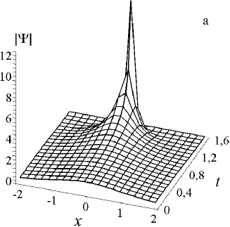
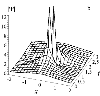
Figure 2:

In Fig. 2a, the function $|\Psi^{+}|$ (56) is shown for the $(1+1)$ space-time and the potential well (${kx^{2}}/{2}$, $k>0$) of the oscillator form in (46) with $\hbar=1$. It can be seen that the solution, being localized at the initial time, is focused within the time interval $(0,\pi/2)$ (in the process of evolution) and collapses. The GPE with an external field was used to describe the dispersion and diffraction of nonlinear waves [32]. The collapse phenomenon was studied in [32] by numerical simulations. The numerical results qualitatively correlate with those obtained by analytic asymptotic methods. The asymptotic solution (53) describes the system for any $T$ within a finite time interval $[0,T]$. If the time interval is short enough, the evolution can end before the collapse occurs.

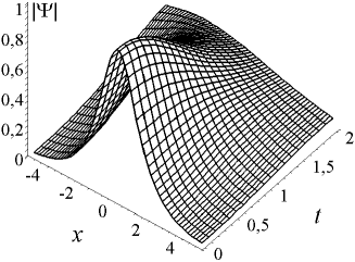
Figure 3:

The function (56) is $\pi$-periodic and its graph is given in Fig. 2b. The term $(-\hbar/2)\ln|\cos(t)|$ in the argument of hyperbolic cosine in equation (56) shifts the function centroid (56) within the time interval $0<t<{\pi}/{2}$. Throughout the evolution time, this gives rise to oscillations of the function maximum about the plane $x=0$.

For the potential hill of the oscillator form (${kx^{2}}/{2}$, $k<0$) in equation (46), the state of the system in the $(1+1)$ space-time is described by $\Psi^{-}$. Let us choose the initial condition for the function $\Psi^{-}$ the same as for $\Psi^{+}$. Then the dynamics of the system is characterized by defocusing and exponential damping (see Fig. 3). The term $(-\hbar/2)\ln(\mathop{\rm ch}(t))$ in the argument of hyperbolic cosine in (57) shifts the function centroid in the negative direction of $x$.

Consider the $(2+1)$-dimensional case. For the functions (52) put $\vec{P}(0)=0$, $\vec{x}(0)=0$, $\pi_{0}=1$, $\sigma_{1}(0)=0$, then we have

$$|\Psi^{+}(\vec{x},t,\hbar)|=|\cos(t)|^{-1}\mathop{\rm ch}{}^{-1}\left[\frac{1}{\hbar}\left(\frac{x_{1}}{\cos(t)}+\frac{x_{2}^{2}}{2}-\frac{\hbar}{2}\ln|\cos(t)|\right)\right],$$ (58)

$$\displaystyle|\Psi^{-}(\vec{x},t,\hbar)|=|\mathop{\rm ch}(t)|^{-1}\mathop{\rm ch}{}^{-1}\left[\frac{1}{\hbar}\left(\frac{x_{1}}{\mathop{\rm ch}(t)}+\frac{x_{2}^{2}}{2}-\frac{\hbar}{2}\ln\mathop{\rm ch}(t)\right)\right].$$ (59)

The functions (58) and (59) coincide at $t=0$. The initial graph of the functions (58) and (59) is presented in Fig. 4a. Figs. 4b,c show the graphs of function (58) for $t=1.2$ and of the function (59) for $t=2$, respectively.

  

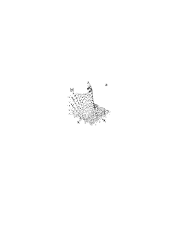
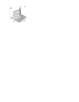
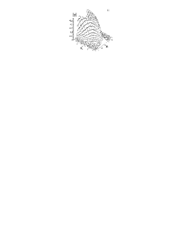
Figure 4:

The solution considered is localized about the parabola with the vertex at the point $\vec{P}\left({t}\right)=0$, $\vec{X}\left({t}\right)=0$ of phase space. In the course of evolution of $|\Psi^{+}|$, the parabola branches disperse and at $t=\pi/2$ it transforms into a straight line. The inverse behavior of the parabola takes place for the evolution of $|\Psi^{-}|$: the parabola branches converge for an infinite time. The amplitude of the functions $|\Psi^{\pm}|$ behaves, in the direction along the coordinate $x$, as in the $(1+1)$-dimensional case.

6 Conclusion remarks

The asymptotics obtained, equation (6), can be regarded as a necessary step in the construction of a global semiclassical asymptotic solution to the GPE (2). It may be supposed that the functions (6) describe the behavior of an element of the global solution in the neighborhood of a ray along the normal $\vec{\pi}$ (Fig. 1) to the (closed) surface about which the global solution is concentrated. Substantiation of these global asymptotics for finite times $t\in[0,T]$, $T=\mbox{\rm const}$, is a special nontrivial mathematical problem. This problem is concerned with obtaining a priori estimates for the solution of a nonlinear equation, which are uniform in parameter $\hbar\in]0,1]$ and is beyond the scope of the present work. Note that, in view of the heuristic considerations given in [15], it seems that the difference between the exact and the constructed formal asymptotic solution can be found with the use of method developed in [15, 23].

The technique of construction of semiclassical asymptotics developed in Section 4 provides a way for solving the problem of correspondence between the classical and quantum results for quantum systems described by nonlinear equations, namely, via finding solutions to the dynamic system (26) and (28). For nonlinear systems this problem differs from the relevant problem in the linear quantum mechanics. For linear quantum systems, a correct formal transition from the quantum theory to the classical one requires imposing special limitations on the quantum states (their semiclassical concentration). The states not satisfying these limitations are regarded as “essentially quantum”, and those satisfying them are considered “near to classical”. Thus, the dynamics of the classical objects obtained is described by the classical Hamiltonian equations no matter the domain where the wave function is concentrated (whether it be a point, a curve, or a surface). The study of the dynamic system (26) and (28) is a separate mathematical subject for research. For example, the Hamiltonian or Poissonian formalisms as applied to this system are of interest.

The construction of “transverse” evolution operator given in Section 4 allows one not only to obtain semiclassical asymptotics but also to construct approximate symmetry operators of special type acting in the class of ${\mathcal{S}}_{\hbar}^{t}$ functions under consideration. Such operators can be naturally referred to as semiclassical symmetry operators [33] (see also [12]).

Acknowledgements

The work was supported in part by a Grant of President of the Russian Federation (No. NSh-1743.2003.2).

References

[1] Gross E.P., Structure of a quantized vortex
in boson systems, Nuovo Cimento, 1961, V.20, N 3, 454–477.
[2] Pitaevskii L.P., Vortex lines in
an imperfect Bose gas, Zh. Eksper. Teor. Fiz., 1961, V.40,
646–651.
[3] Zakharov V.E., Manakov S.V.,
Novikov S.P., Pitaevsky L.P., Theory of solitons: the inverse
scattering method, Moscow, Nauka, 1980 (English transl.: New
York, Plenum, 1984).
[4] Zakharov V.E., Shabat A.B.,
Exact theory of two-dimensional self-focusing and one-dimensional
self-modulation of waves in non-linear media, Zh. Eksper.
Teor. Fiz., 1971, V.61, 118–134 (English transl.: Soviet Physics JETP, 1972, V.34, 62–69).
[5] Hasegawa A., Tappert F., Transmission of
stationary nonlinear optical pulse in dispersive dielectric
fibres, Appl. Phys. Lett., 1973, V.23, 171–172.
[6] Mollenauer L.F., Stolen R.H., Gordon J.P., Experimental
observation of picosecond pulse narrowing and solitons in optical
fibres, Phys. Rev. Lett., 1980, V.45, 1095–1098.
[7] Yuen H.C., Lake B.M., Nonlinear dynamics of deep-water
gravity waves, Advances in Applied Mechanics, 1982, V.22,
67–229.
[8] Dalfovo F., Giorgini S., Pitaevskii L.,
Stringary S., Theory of Bose–Einstein condensation in traped
gases, Rev. Mod. Phys., 1999, V.71, N 3, 463–512.
[9] Zakharov V.E., Synakh V.S.,
On the character of a singularity under self-focusing, Zh.
Eksper. Teor. Fiz., 1975, V.68, 940–947.
[11] Belov V.V., Trifonov A.Yu., Shapovalov A.V., The
trajectory-coherent approximation and the system of moments for
the Hartree type equation, Int. J. Math. and Math. Sci.,
2002, V.32, N 6, 325–370.
[12] Lisok A.L., Trifonov A.Yu., Shapovalov A.V.,