Discrete Lagrangian field theories on Lie groupoids

Abstract

We present a geometric framework for discrete classical field theories, where fields are modeled as “morphisms” defined on a discrete grid in the base space, and take values in a Lie groupoid. We describe the basic geometric setup and derive the field equations from a variational principle. We also show that the solutions of these equations are multisymplectic in the sense of Bridges and Marsden. The groupoid framework employed here allows us to recover not only some previously known results on discrete multisymplectic field theories, but also to derive a number of new results, most notably a notion of discrete Lie-Poisson equations and discrete reduction. In a final section, we establish the connection with discrete differential geometry and gauge theories on a lattice.

1 Introduction

The idea of studying mechanical systems on Lie groupoids first arose in the context of discrete dynamical systems when Moser and Veselov (see [30]) considered the pair groupoid $Q\times Q$ as a discretization of the tangent bundle $TQ$ and used it in their study of discrete integrable systems. Their idea was subsequently used by Weinstein [35], who introduced (among other things) Lagrangian mechanics on an arbitrary Lie groupoid, established a suitable variational principle for it and laid the foundations of discrete reduction.

The theme of mechanics on a Lie groupoid was then picked up again in [24], in which the authors extended Weinstein’s approach by fully exploring the geometry of the various prolongation bundles associated to the groupoid. They gave a direct construction of the Poincaré-Cartan forms and the Legendre transformations, proved the symplecticity of the discrete flow and made the connection with numerous examples of discrete mechanical systems that had been studied before (see [5, 25, 35] and the references therein).

Meanwhile, the foundational idea of Moser and Veselov of replacing $TQ$ by the discretization $Q\times Q$, was extended to the case of field theories by Marsden, Patrick and Shkoller in [26]. Their objective was a systematic study of the geometry of discrete multisymplectic field theories, aimed at the design of robust numerical integrators that conserve an appropriate notion of “symplecticity”. The symplectic nature of their discrete field theories is a consequence of the variational structure and is expressed in terms of a set of distinct one-forms $\theta_{L}^{i}$, called Poincaré-Cartan forms, such that $\sum_{i}\theta_{L}^{i}=\mathrm{d}L$, and they observed that symplectic discretization schemes indeed yield superior results.

A similar approach, but aimed instead at Hamiltonian multisymplectic PDEs, was proposed in [11], based on Bridges’ notion of multisymplecticity in [8, 10] (see also [9, 22]), and again it was observed that multisymplectic discretizations indeed have remarkable energy and momentum conservation properties. Moreover, they showed that a number of classical numerical schemes such as the Euler or Preissman box scheme have a natural interpretation as multisymplectic integrators.

The objective of this paper is to establish the discrete counterpart of Lagrangian multisymplectic field theory, in the case where the discrete fields take values in an arbitrary Lie groupoid. In doing so, we extend both discrete Lagrangian field theory, as treated in [26], as well as mechanics on Lie groupoids [24]. We use techniques from groupoid mechanics and show how they can be generalized quite easily to field theories. In doing so, we develop some new insights into some of the constructions in [26]. Finally, we present a number of new results which require the full machinery developed here. The most notable example is a discrete version of the Lie-Poisson equations for field theories. We finish by presenting some remarks on discrete differential geometry, as it turns out that our way of modeling discrete fields is reminiscent of the way in which discrete connections are usually introduced.

2 Discrete mechanics on Lie groupoids

In this section, we recall some of the basic definitions and results from the theory of Lie groupoids and algebroids. It is not our intention to give a detailed introduction to the suject: for a more in-depth overview, the reader is referred to [23] and the references therein. We will also recall some of the constructions in [24] that will be generalized in the next sections. We note that the definition of a groupoid used here agrees with [24, 35] but differs from [33] with respect to the order of writing the product $gh$.

2.1 Lie groupoids

A groupoid is a set $G$ with a partial multiplication $m$, a subset $Q$ of $G$ whose elements are called identities, two surjective maps $\alpha,\beta:G\rightarrow Q$ (called source and target maps respectively), which both equal the identity on $Q$, and an inversion mapping $i:G\rightarrow G$. A pair $(g,h)$ is said to be composable if the multiplication $m(g,h)$ is defined; the set of composable pairs will be denoted by $G_{2}$. We will denote the multiplication $m(g,h)$ by $gh$ and the inversion $i(g)$ by $g^{-1}$. In addition, these data must satisfy the following properties, for all $g,h,k\in G$:

1. the pair $(g,h)$ is composable if and only if $\beta(g)=\alpha(h)$, and then $\alpha(gh)=\alpha(g)$ and $\beta(gh)=\beta(h)$;

2. if either $(gh)k$ or $g(hk)$ exists, then both do, and they are equal;

3. $\alpha(g)$ and $\beta(g)$ satisfy $\alpha(g)g=g$ and $g\beta(g)=g$;

4. the inversion satisfies $g^{-1}g=\beta(g)$ and $gg^{-1}=\alpha(g)$.

On a groupoid, we have a natural notion of left translation $l_{g}$, defined as $l_{g}(h)=gh$, for any $h\in G$ such that $\alpha(h)=\beta(g)$. There is a similar definition for a right translation $r_{g}$.

A morphism of groupoids is a pair of maps $\phi:G\rightarrow G^{\prime}$ and $f:Q\rightarrow Q^{\prime}$ satisfying $\alpha^{\prime}\circ\phi=f\circ\alpha$, $\beta^{\prime}\circ\phi=f\circ\beta$ and such that $\phi(gh)=\phi(g)\phi(h)$ whenever $(g,h)$ is composable. Note that $(\phi(g),\phi(h))$ is a composable pair whenever $(g,h)$ is composable.

A Lie groupoid is a groupoid for which $G$ and $Q$ are differentiable manifolds, with $Q$ a closed submanifold of $G$, the maps $\alpha,\beta,m$ and $i$ are smooth and $\alpha$ and $\beta$ are submersions. We denote by $\mathcal{F}^{\alpha}(g)$ the $\alpha$-fibre through $g\in G$, i.e. $\mathcal{F}^{\alpha}(g)=\alpha^{-1}(\alpha(g))$, with a similar definition for $\mathcal{F}^{\beta}(g)$. As $\alpha$ and $\beta$ are submersions, both $\mathcal{F}^{\alpha}(g)$ and $\mathcal{F}^{\beta}(g)$ are closed submanifolds of $G$.

Any Lie group $G$ can be considered as a Lie groupoid over a singleton $\{e\}$, where the anchors $\alpha,\beta$ map any element onto $x$ and the multiplication is defined everywhere. Another example of a Lie groupoid is the pair groupoid $Q\times Q$, where $\alpha(q_{1},q_{2})=q_{1}$, $\beta(q_{1},q_{2})=q_{2}$, and multiplication is defined as $(q_{1},q_{2})\cdot(q_{2},q_{3})=(q_{1},q_{3})$. For other, less trivial examples, we refer to the works mentioned above.

2.2 Lie algebroids

A Lie algebroid over $Q$ is a vector bundle $\tau:E\rightarrow Q$ together with a vector bundle map $\rho:E\rightarrow TQ$ (called the anchor map of the Lie algebroid) and a bracket $[\cdot,\cdot]:\mathrm{Sec}(E)\times\mathrm{Sec}(E)\rightarrow\mathrm{Sec}(E)$ defined on the sections of $\tau$, such that

1. $\mathrm{Sec}(E)$ is a real Lie algebra with respect to $[\cdot,\cdot]$;

2. $\rho([\phi,\psi])=[\rho(\phi),\rho(\psi)]$, for all $\phi,\psi\in\mathrm{Sec}(E)$, where the bracket on the right-hand side is the usual Lie bracket of vector fields on $Q$ and we write the composition $\rho\circ\phi$ as $\rho(\phi)$;

3. $[\phi,f\psi]=f[\phi,\psi]+\rho(\phi)(f)\psi$, for all $\phi,\psi\in\mathrm{Sec}(E)$ and $f\in C^{\infty}(Q)$.

The Lie algebroid structure allows us to define an exterior differential $\mathrm{d}_{E}$ on the space of sections of $\bigwedge^{\ast}(E^{\ast})$, as follows: for functions $f\in C^{\infty}(Q)$, we put $\mathrm{d}_{E}f(v)=\rho(v)f$, for $v\in E$, while for sections $\theta$ of $\bigwedge^{k}(E^{\ast})$, we define $\mathrm{d}_{E}\theta$ by

$$\mathrm{d}_{E}\theta(v_{0},v_{1},\ldots,v_{k})=\sum_{i}\rho(v_{i})\theta(v_{0},\ldots,\hat{v}_{i},\ldots,v_{k})\\ +\sum_{i<j}(-1)^{i+j}\theta([v_{i},v_{j}],v_{0},\ldots,\hat{v}_{i},\ldots,\hat{v}_{j},\ldots,v_{k}).$$

It can be shown that $\mathrm{d}_{E}$ is nilpotent: $\mathrm{d}_{E}^{2}=0$.

To any Lie groupoid $G$ over $Q$ one can associate a Lie algebroid $\tau:AG\rightarrow Q$ as follows. At each point $x\in Q$, the fibre $A_{x}G$ is the vector space $V_{x}\alpha=\ker T_{x}\alpha$ and the anchor map $\rho$ on $A_{x}G$ is identified with the restriction of $T_{x}\beta$ to $V_{x}\alpha$. In order to define the bracket on the space of sections, we note that there exists a bijection between sections of $\tau$ and left- and right-invariant vector fields on $G$. More specifically, if $v$ is a section of $\tau$, then the left- and right-invariant vector fields are denoted as $v^{L}$ and $v^{R}$ respectively, and defined by

$$v^{L}(g)=T_{\beta(g)}l_{g}(v_{\beta(g)})\quad\mathrm{and}\quad v^{R}(g)=T_{\alpha(g)}(r_{g}\circ i)(v_{\alpha(g)}).$$ (1)

Let $v$ and $w$ be sections of $\tau$. The bracket $[v,w]$ is then defined by noting that $[v^{L},w^{L}]$ is again a left-invariant vector field, and putting

$$[v,w]^{L}=[v^{L},w^{L}].$$

We remark that our definition of $v^{R}$ differs in sign from the one used in [24].

Conversely, we say that a Lie algebroid $\tau:E\rightarrow Q$ is integrable whenever one can find a Lie groupoid such that $E$ is its associated Lie algebroid. It has been known for some years that not all Lie algebroids are integrable. Necessary and sufficient conditions for integrability have been given in [16].

The Lie algebroid of a Lie group $G$ is just its Lie algebra. The Lie algebroid of the pair groupoid $Q\times Q$ is the tangent bundle $TQ$.

Remark 2.1.

For a given section $v$ of $\tau$, we have denoted the corresponding left- and right-invariant vector fields as $v^{L}$ and $v^{R}$, respectively. We will also use this notation for the pointwise operation, by denoting, for $v_{x}$ an element of $A_{x}G$ and $g\in\alpha^{-1}(x)\subset G$, the left translated vector $T_{x}l_{g}(v_{x})$ as $(v_{x})^{L}(g)$, and similarly the right translated vector $T_{x}(r_{g}\circ i)(v_{x})$ as $(v_{x})^{R}(g)$. $\diamond$

2.3 Lie algebroid morphisms

Consider two vector bundles $\tau^{\prime}:E^{\prime}\rightarrow Q^{\prime}$ and $\tau:E\rightarrow Q$, and let $(\Phi,\varphi)$ be a vector bundle map from $\tau^{\prime}$ to $\tau$. Let $\theta$ be a section of $\bigwedge^{k}(E^{\ast})$. Then the pullback of $\theta$ by $(\Phi,\varphi)$ is the section $\Phi^{\star}\theta$ of $\bigwedge^{k}(E^{\prime\ast})$ defined as

$$(\Phi^{\star}\theta)_{q}(v_{1},\ldots,v_{k})=\theta_{\varphi(q)}(\Phi(v_{1}),\ldots,\Phi(v_{k})),\quad v_{1},\ldots,v_{k}\in E_{q}.$$

Note that we used a “star” $\star$ instead of an “asterisk” $\ast$ to denote the pullback, which should serve as a reminder that we consider the pullback of $\theta$ by a bundle map rather than by an arbitrary differentiable map from $E^{\prime}$ to $E$.

Now, assume that both $\tau$ and $\tau^{\prime}$ are equipped with the structure of a Lie algebroid over $Q$. In this case, a vector bundle map $(\Phi,\varphi)$ is said to be a morphism of Lie algebroids if for each section $\theta$ of $\bigwedge^{k}(E^{\ast})$,

$$\Phi^{\star}\mathrm{d}_{E}\theta=\mathrm{d}_{E^{\prime}}\Phi^{\star}\theta,$$

where $\mathrm{d}_{E}$ and $\mathrm{d}_{E^{\prime}}$ are the differentials on $E$ and $E^{\prime}$, respectively. In other words, $(\Phi,\varphi)$ is a chain map. In [20, 28, 29], a number of equivalent conditions are investigated for a bundle map to be a morphism of Lie algebroids.

2.4 The prolongation of a Lie groupoid over a fibration

Let $G$ be a Lie groupoid over a manifold $Q$ with source and target maps $\alpha$ and $\beta$ and consider a fibration $\pi:P\rightarrow Q$. The prolongation $P^{\pi}G$ is the Lie groupoid over $P$ defined as

$$P^{\pi}G=\{(g;p_{1},p_{2})\in G\times P\times P:\pi(p_{1})=\alpha(g)\text{ and }\beta(g)=\pi(p_{2})\}.$$

Alternatively, $P^{\pi}G$ is defined by means of the following commutative diagram:

(2)

It can be shown that $P^{\pi}G$ is a Lie groupoid over $P$, with source and target mappings $\alpha^{\pi},\beta^{\pi}:P^{\pi}G\rightarrow P$ defined as

$$\alpha^{\pi}(g;p_{1},p_{2})=p_{1}\quad\mathrm{and}\quad\beta^{\pi}(g;p_{1},p_{2})=p_{2},$$

and with multiplication given by

$$(g;p_{1},p_{2})(h;p_{2},p_{3})=(gh;p_{1},p_{3}).$$

Note that $\alpha^{\pi}(h;p_{2},p_{3})=\beta^{\pi}(g;p_{1},p_{2})$ implies that $\alpha(h)=\beta(g)$. Finally, the inversion mapping is defined as

$$i:(g;p_{1},p_{2})\mapsto(g^{-1};p_{2},p_{1}),$$

and we can regard $P$ as a subset of $P^{\pi}G$ via the identification $p\mapsto(\pi(p);p,p)$.

2.4.1 The prolongation $PG$

There is one particular prolongation that will play a significant role in what follows. It is obtained by taking for the fibration $\pi:P\rightarrow Q$ in (2) the Lie algebroid projection $\tau:AG\rightarrow Q$ to obtain

$$P^{\tau}G\subset G\times AG\times AG$$

which, henceforth, we also simply denote as $PG$. We recall that $PG$ consists of triples $(g;v_{x},w_{y})$, where $g\in G$, $v_{x}\in A_{x}G$, $w_{y}\in A_{y}G$, and $x=\alpha(g)$, $y=\beta(g)$. It is pointed out in [24, 33] that $PG$ is isomorphic as a vector bundle over $G$ to the direct sum $V\beta\oplus V\alpha$, where $V\alpha$ is the subbundle of $TG$ consisting of $\alpha$-vertical vectors (and similarly for $V\beta$); the isomorphism $\Theta:PG\rightarrow V\beta\oplus V\alpha$ is defined by

$$\Theta(g;u_{\alpha(g)},v_{\beta(g)})=(T(r_{g}\circ i)(u_{\alpha(g)}),Tl_{g}(v_{\beta(g)})).$$ (3)

It should also be remarked that $PG$ is a vector bundle over $G$, and in fact, $PG$ can be endowed with the structure of an integrable Lie algebroid over $G$, where the anchor map $\hat{\rho}:PG\rightarrow TG$ is given by

$$\hat{\rho}:(g;u_{\alpha(g)},v_{\beta(g)})\mapsto T(r_{g}\circ i)(u_{\alpha(g)})+Tl_{g}(v_{\beta(g)})=(u_{\alpha(g)})^{R}(g)+(v_{\beta(g)})^{L}(g).$$

Given a pair of sections $u,v$ of $AG$, one can construct a section of $PG\rightarrow G$, shortly denoted by $(u,v)$, by considering the map $g\mapsto(g;u_{\alpha(g)},v_{\beta(g)})$. The Lie bracket of sections of $PG$ is then determined by the following definition:

$$[(u,v),(u^{\prime},v^{\prime})]_{PG}=([u,u^{\prime}],[v,v^{\prime}]),$$

where $u,u^{\prime},v,v^{\prime}$ are sections of $AG$ (see [24, Thm. 3.1]).

2.5 The prolongation of a Lie algebroid over a fibration

Let $\tau:E\rightarrow Q$ be a Lie algebroid and consider a fibration $\pi:P\rightarrow Q$. The prolongation $P^{\pi}E$ is the Lie algebroid over $P$ defined as

$$P^{\pi}E=\{(a,v)\in E\times TP:\rho(a)=T\pi(v)\},$$

or by the following commutative diagram as

(4)

We denote by $\hat{\pi}:P^{\pi}E\rightarrow P$ the map defined as $\hat{\pi}(a,v)=\pi_{TP}(v)$, where $\pi_{TP}:TP\rightarrow P$ is the tangent bundle projection of $P$. It can be shown that $\hat{\pi}:P^{\pi}E\rightarrow P$ can be given the structure of a Lie algebroid (see [20, 27, 33]).

2.5.1 The prolongations $P^{\tau}(AG)$ and $P^{\tau^{\ast}}(AG)$

Let $G$ be a Lie groupoid over a manifold $Q$ with Lie algebroid $\tau:AG\rightarrow Q$. By taking for the fibration $\pi$ underlying diagram (4) the map $\tau$, we obtain the prolongation $P^{\tau}(AG)$. It is very useful to think of $P^{\tau}(AG)$ as a sort of Lie algebroid analogue of the tangent bundle to $AG$. Indeed, $P^{\tau}(AG)$ can be equipped with geometric objects, such as a Liouville section and a vertical endomorphism, which have their counterpart in tangent bundle geometry.

Similarly, by taking for $\pi:P\rightarrow Q$ the dual bundle $\tau^{\ast}:A^{\ast}G\rightarrow Q$, we obtain the prolongation $P^{\tau^{\ast}}(AG)$, which is a Lie algebroid over $A^{\ast}G$ and should be thought of as the Lie algebroid analogue of the tangent bundle to $A^{\ast}G$. Just as any cotangent bundle is equipped with a canonical one-form, there exists a canonical section

$$\theta:A^{\ast}G\rightarrow\left[P^{\tau^{\ast}}(AG)\right]^{\ast},$$

defined as follows: for $\alpha\in A^{\ast}G$ and $(v,X_{\alpha})\in(P^{\tau^{\ast}}(AG))_{\alpha}$, we put $\theta_{\alpha}(v,X_{\alpha})=\alpha(v)$. In the case that $G$ is the pair groupoid $Q\times Q$, we have that $A^{\ast}G=T^{\ast}Q$ and we obtain the usual canonical one-form on $T^{\ast}Q$.

It was shown in [20] that $P^{\tau}(AG)$, the prolongation of the Lie algebroid $AG$, is isomorphic to $A(PG)$, the Lie algebroid associated to the prolongation Lie groupoid $PG$.

2.5.2 The prolongations $P^{\alpha}(AG)$ and $P^{\beta}(AG)$

Associated to the source and target mappings $\alpha$ and $\beta$ of a groupoid $G$ there are two prolongations $P^{\alpha}(AG)$ and $P^{\beta}(AG)$, whose fibres over $G$ are defined as follows: for each $g\in G$, put

$$P^{\alpha}_{g}(AG)=\{(v_{\alpha(g)},X_{g})\in A_{\alpha(g)}G\times T_{g}G:T\tau(v_{\alpha(g)})=T\alpha(X_{g})\}$$

and

$$P^{\beta}_{g}(AG)=\{(v_{\beta(g)},X_{g})\in A_{\beta(g)}G\times T_{g}G:T\tau(v_{\beta(g)})=T\beta(X_{g})\}.$$

Both of these algebroids are integrable: indeed, it follows from the general theory that $P^{\alpha}(AG)$ is isomorphic to the Lie algebroid of the prolongation $P^{\alpha}G$, and similarly for $P^{\beta}(AG)$.

Furthermore, we remark that there are two distinguished mappings from $PG$ (regarded as a Lie algebroid over $G$) into $P^{\alpha}(AG)$ and $P^{\beta}(AG)$, given by

$$A(\Phi^{\alpha}):(u_{\alpha(g)},g,v_{\beta(g)})\mapsto(u_{\alpha(g)},T(r_{g}\circ i)(u_{\alpha(g)})+Tl_{g}(v_{\beta(g)}))\in P^{\alpha}(AG)$$

and

$$A(\Phi^{\beta}):(u_{\alpha(g)},g,v_{\beta(g)})\mapsto(v_{\beta(g)},T(r_{g}\circ i)(u_{\alpha(g)})+Tl_{g}(v_{\beta(g)}))\in P^{\beta}(AG).$$

The notations $A(\Phi^{\alpha})$ and $A(\Phi^{\beta})$ serve as a reminder of the fact that these Lie algebroid maps stem from morphisms between the corresponding groupoids (see [24]).

3 The discrete jet bundle. Discrete fields

Let us now turn to field theory. As is customary in most geometric treatments, we model physical fields as sections of a fibre bundle $\pi:Y\rightarrow X$. This approach has received a lot of attention in the past and we refer to [12, 17, 32] for more information. For the sake of simplicity, we will assume from now on that the base space $X$ of $\pi$ is $\mathbb{R}^{2}$, and that $\pi$ is trivial, i.e. $\pi$ is given by $\pi:\mathbb{R}^{2}\times Q\rightarrow\mathbb{R}^{2}$, where $Q$ is the standard fibre.

It is our aim in this section to present a geometric approach to discrete field theories. A crucial element of this setup is the concept of discrete jet bundle. Before going into details, it is perhaps useful to start with a quick overview of what our construction entails.

3.1 Overview

We will introduce a notion of “discrete jet bundle of $\pi$”, using two essentially different ingredients:

1. The existence of a mesh in $X=\mathbb{R}^{2}$, consisting of a discrete subset $V$ of $X$, whose elements are called vertices, and a set $E$ of edges, which are line segments between pairs of vertices. Associated to such a mesh is a set of faces, where a face $f$ is a region in $\mathbb{R}^{2}$ bounded by edges, and such that there are no edges in the interior of $f$.

2. A groupoid $G$ over the standard fibre $Q$ of $\pi$. This is a new element, and its role will become clear in a moment.

We will define a discrete jet as a mapping which assigns to each edge of the mesh an element of $G$ such that two edges which have a vertex in common are mapped onto composable elements of $G$. We will show that each such mapping gives rise to a groupoid morphism from the pair groupoid $V\times V$ (where $V$ is the set of vertices) to $G$. In section 5.1 we will treat the particular case where $G$ is the pair groupoid $Q\times Q$. In that case, a discrete field is an assignment of an element of $Q$ to each point of a grid in $X$, which is a natural way, used for example in finite-difference methods, to think of discrete fields (see [26]).

The manifold $\mathbb{G}^{k}$

There is another, equivalent, way of thinking of discrete jets, which is closely related to the way in which continuous jets are interpreted. Recall that we considered a trivial bundle $\pi:\mathbb{R}^{2}\times Q\rightarrow\mathbb{R}^{2}$. In this case, the jet bundle $J^{1}\pi$ is isomorphic to the product space $\mathbb{R}^{2}\times J^{1}_{0}(\mathbb{R}^{2},Q)$, where $J^{1}_{0}(\mathbb{R}^{2},Q)$ is the manifold of $1$-jets at $0$ of maps $\varphi:\mathbb{R}^{2}\rightarrow Q$, which is itself isomorphic to the Whitney sum $TQ\oplus TQ$. Incidentally, this is the starting point for the so-called $k$-symplectic (here $k=2$) treatment of field theories (see [18, 31] and the references therein). Hence, a natural interpretation of a jet at a point $x\in\mathbb{R}^{2}$ is as an element of $TQ\oplus TQ$.

Let us now repeat this procedure for the discrete case. We start from the base space $X=\mathbb{R}^{2}$ and a given mesh $(V,E)$. As we argued before, there is a natural definition of the set of faces of this mesh as (connected) regions of the plane bounded by edges. Furthermore, as the edges are represented by pairs of vertices, and faces are defined by specifying their bounding edges, a face is completely determined by its corner vertices $x_{1},\ldots,x_{k}$, where the vertices are ordered in such a way that the bounding edges are $(x_{i},x_{i+1})$ (for $i=1,\ldots,k-1$) and $(x_{1},x_{k})$. Each of the pairs $(x_{i},x_{i+1})$ is a Veselov-type discretization of a tangent vector and, hence a face is a natural way of representing a set of $k-1$ vectors. As soon as $k>3$, this set can never be linearly independent. However, it turns out that this makes essentially no difference for the discrete approach, and might even have certain benefits in the design of numerical methods (see [26, p. 42]). We will consider in general only meshes in which each face has the same number of edges, which we denote henceforth as $k$.

Recall that in the continuous case, we interpreted jets as elements of $TQ\oplus TQ$ by considering the values they take on the standard basis of $\mathbb{R}^{2}$. Let us now define a discrete jet as an assignment of $k$ points in $Q$ to any face $\{x_{1},\ldots,x_{k}\}$ of the mesh, in other words: a $k$-tuple $\{q_{1},\ldots,q_{k}\}$ of points in $Q$ (together with the face $\{x_{1},\ldots,x_{k}\}$). Hence the fibre part of our space (the part involving only $Q$) of jets is really a discretization of $TQ\oplus\cdots\oplus TQ$ ($k$ times).

As a slight generalization, we can easily replace the pair groupoid $Q\times Q$ by an arbitrary groupoid $G$ over $Q$: in this case, we are led to the study of a similar manifold $\mathbb{G}^{k}$ (consisting of “faces” in $G$, to be specified later), which is the discrete counterpart of $AG\oplus\cdots\oplus AG$.

In proposition 3.8, we will show how both points of view, i.e. discrete jets on the one hand and the manifold $\mathbb{G}^{k}$ on the other hand, are related.

3.2 Discretizing the base space

3.2.1 The mesh

To discretize $X=\mathbb{R}^{2}$, we will use the concept of a mesh embedded in $X$. Intuitively, such a mesh consists of a discrete subset $V$ of $X$ together with a number of relations specifying which points of $V$ “belong together”. This can be made more rigourous by means of some elementary concepts from graph theory, which we now review.

A graph is a pair of sets $(V,E)$ such that $E$ is a subset of $V\times V$. In contrast to what is usually assumed in graph theory, we will allow $V$ and $E$ to be (countably) infinite. The elements of $V$ are called vertices, while those of $E$ are called edges. Note that the edges in $E$ are undirected.

A graph is simple if there is at most one edge connecting each pair of distinct vertices. In this case, let us represent an edge $e\in E$ by its incident vertices as $e\rightsquigarrow\{x,y\}$. A path between two vertices $x$ and $y$ is a sequence of edges $\{x,p_{1}\},\{p_{1},p_{2}\},\ldots,\{p_{l},y\}$. A graph is said to be connected if there exists a path between any two vertices. In the sequel, we will only consider connected, simple graphs, with the additional condition that there are no “loops”, i.e. no edges $e$ whose incident vertices coincide.

A planar graph is a graph $(V,E)$ where $V$ is a subset of $\mathbb{R}^{2}$ and the edges are curves in $E$ connecting pairs of vertices such that if any two edges intersect, they do so in a common vertex. For a planar graph, there is a notion of face, defined as follows. Consider the geometric realisation $|E|$ of $(V,E)$, which is just the union of all edges. The complement $\mathbb{R}^{2}\backslash|E|$ of $|E|$ is a disconnected set, whose connected components are the faces of the planar graph $(V,E)$. A face is therefore a region in the plane, bounded by a number of edges.

The degree of a face is defined as the number of edges that make up the boundary of that face. Dually, the degree of a vertex is defined as the number of edges arriving in that vertex.

Definition 3.1.

A mesh in $X=\mathbb{R}^{2}$ is a simple and connected planar graph $(V,E)$ in $X$ such that the following conditions are satisfied:

1. the edges are realised as segments of straight lines in $\mathbb{R}^{2}$;

2. the degree of the faces is constant and equal to some natural number $k>2$;

3. the degree of the vertices is always larger than two.

It has to be stressed that the nature of this graph is left entirely unspecified and should be dictated by the problem under scrutiny. Throughout this text, we will illustrate our theory from time to time using some elementary meshes, of which the covering of $\mathbb{R}^{2}$ by quadrangles, as in figure 1, is the most straightforward. This mesh was also used in [26].

A few remarks concerning the above definition are in order. The fact that, given a mesh $(V,E)$, the elements of $E$ are realised as straight line segments, implies that each edge is determined by its begin and end vertex. Similarly, a face $f$ is determined by its $k$ bounding edges $e_{1},\ldots,e_{k}$, each of which can be represented as a pair of vertices $e_{i}=\{x_{i},x_{i+1}\}$ (where $x_{k+1}=x_{1}$), and, hence, $f$ is determined by specifying the set of its “corner” vertices:

$$f\rightsquigarrow\{x_{1},\ldots,x_{k}\}.$$

The set of all faces associated to a mesh $(V,E)$ will be denoted by $F$. One can envisage a more general situation in which the edges are allowed to be more general curves.

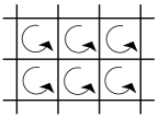
Figure 1: Square mesh in $\mathbb{R}^{2}$, with counterclockwise orientation.

Remark 3.2.

In a recent paper [36] on lattice gauge theories, the author introduces a discretization of space-time by means of a hypothetical “$n$-graph” structure, which is a list of data $X_{0},X_{1},X_{2},\ldots$, where $X_{0}$ is a set of vertices, $X_{1}$ a set of edges, and so on, with sets $X_{i}$ of higher-dimensional objects. These sets have to specify various incidence relations, the nature of which is still not entirely clear. However, the concepts of $n$-graphs or $n$-complexes (weaker versions of $n$-graphs) would be useful in generalising our theory to the case where the base space is no longer two-dimensional or Euclidian. $\diamond$

3.2.2 The local groupoid $E$

In order to bring to the fore the algebraic character of the set of edges $E$ of a given mesh $(V,E)$, we construct a new set $E^{\prime}$, whose elements are ordered pairs $(x,y)\in V\times V$ satisfying the following axioms:

1. $(x,x)\in E^{\prime}$ for all $x\in V$;

2. if $\{x,y\}$ is an element of $E$, then $(x,y)\in E^{\prime}$ and $(y,x)\in E^{\prime}$.

The important difference between $E$ and $E^{\prime}$ is that the elements of $E$ are undirected edges, whereas the elements of $E^{\prime}$ are directed. As we will no longer have a use for $E$, no confusion can arise if we, henceforth, denote $E^{\prime}$ simply by $E$.

If we define the source and target mappings $\alpha_{X},\beta_{X}:E\rightarrow V$ in the usual way as $\alpha_{X}(x,y)=x$ and $\beta_{X}(x,y)=y$, then $E$ is a subset of the pair groupoid $V\times V$, satisfying all but one of the axioms of a discrete groupoid: if $e_{1}=(x,y)$ and $e_{2}=(y,z)$ are elements of $E$ such that $\beta_{X}(e_{1})=\alpha_{X}(e_{2})$, then the multiplication $e_{1}\cdot e_{2}$, defined as $e_{1}\cdot e_{2}=(x,z)$, is an element of $V\times V$ but not necessarily of $E$.

This is strongly reminiscent of the concept of local groupoid introduced by Van Est in [34] in the context of Lie groupoids as, roughly speaking, differentiable groupoids in which the condition $\beta(e_{1})=\alpha(e_{2})$ is necessary but not sufficient for the product $e_{1}\cdot e_{2}$ to exist. Even though in its original definition this concept makes no sense for discrete spaces, the name is nevertheless quite appropriate and so we will continue to refer to $E$ as a local groupoid.

3.2.3 The set of $k$-gons $\mathbb{X}^{k}$

We now introduce the set of $k$-gons $\mathbb{X}^{k}$. The elements of this set are the faces of the mesh, but with a consistent orientation. Indeed, the natural orientation of $X=\mathbb{R}^{2}$ allows us to write down the edges of each face $f$ in (say) counterclockwise direction:

$$f=(x_{k},x_{1}),(x_{1},x_{2}),\ldots,(x_{k-1},x_{k}).$$

We now introduce $\mathbb{X}^{k}$ as the set of all faces, considered as $k$-tuples of edges written down in the counterclockwise direction:

$$\mathbb{X}^{k}=\left\{\big{(}(x_{k},x_{1}),(x_{1},x_{2}),\ldots,(x_{k-1},x_{k})\big{)}\quad\mathrm{where}\>\{x_{1},\ldots,x_{k}\}\in F\right\}.$$

We will also refer to the elements of $\mathbb{X}^{k}$ as $k$-gons and denote them as $[x]:=((x_{k},x_{1}),(x_{1},x_{2}),\ldots,(x_{k-1},x_{k}))$. To refer to the $i$th component of a $k$-gon $[x]$, we will use the subscript notation: $[x]_{1}=(x_{k},x_{1})$ and $[x]_{i}=(x_{i-1},x_{i})$ for $i=2,\ldots,k$. In the following, we will assume that the indices are defined “modulo $k$, plus one”, which allows us to write $[x]_{i}=(x_{i-1},x_{i})$, for all $i=1,\ldots,k$.

It is useful to note that a $k$-gon is not changed by a cyclic permutation of its elements and that the common edge of two adjacent $k$-gons is traversed in opposite directions.

Example 3.3.

In the example given in figure 1, the degree of each face is exactly four as each face is made up of four edges. The elements of $\mathbb{X}^{4}$ are the faces with the counterclockwise orientation indicated on the figure.

3.3 The discrete jet space $\mathbb{G}^{k}$

We now complete our programme of discretizing the jet bundle of $\pi$ by constructing over the fibre $Q$ a structure $\mathbb{G}^{k}$ similar to $\mathbb{X}^{k}$. The elements of $\mathbb{G}^{k}$ are $k$-gons in $G$, each of which is an approximation of a frame by $k$ groupoid elements.

Definition 3.4.

The discrete jet bundle is the manifold $\mathbb{G}^{k}$ consisting of all ordered $k$-tuples $(g_{1},\ldots,g_{k})\in G\times\cdots\times G$ such that

$$(g_{1},g_{2}),(g_{2},g_{3}),\ldots,(g_{k},g_{1})\in G_{2}\quad\mathrm{and}\quad g_{1}\cdot g_{2}\cdots g_{k}=\alpha(g_{1})(=\beta(g_{k})).$$

Elements of $\mathbb{G}^{k}$ will be denoted as $[g]=(g_{1},\ldots,g_{k})$, and, with the “modulo” convention introduced above, a subscript will be used to refer to the individual components: $[g]_{i}=g_{i}$. Note that, whereas $\mathbb{X}^{k}$ is a discrete set due to its compatibility with the mesh, $\mathbb{G}^{k}$ is a smooth manifold and $\dim\mathbb{G}^{k}\geq\dim G$.

The discrete jet bundle $\mathbb{G}^{k}$ can be equipped with the following two operations:

1. the inverse of a given $k$-gon $[g]$, denoted as $[g]^{-1}$ and defined as

   $$[g]^{-1}=(g_{k}^{-1},g_{k-1}^{-1},\ldots,g_{1}^{-1});$$

2. a collection of $k$ mappings $\alpha^{(i)}:\mathbb{G}^{k}\rightarrow Q$, called generalized source maps and defined as $\alpha^{(i)}([g])=\alpha(g_{i})$.

3.4 Discrete fields

The idea of a “discrete field” can be expressed in terms of a mapping that associates to each edge (i.e. to each element of the set $E$, in the extended sense of subsection 3.2.2) an element of the groupoid $G$, and to each vertex in $V$ a unit of $G$, such that whenever two edges are composable, so are their images.

Definition 3.5.

A discrete field is a pair $\phi=(\phi_{(0)},\phi_{(1)})$, where $\phi_{(0)}$ is a map from $V$ to $Q$ and $\phi_{(1)}$ is a map from $E$ to $G$ such that

1. $\alpha(\phi_{(1)}(x,y))=\phi_{(0)}(x)$ and $\beta(\phi_{(1)}(x,y))=\phi_{(0)}(y)$;

2. for each $(x,y)\in E$, $\phi_{(1)}(y,x)=[\phi_{(1)}(x,y)]^{-1}$;

3. for all $x\in V$, $\phi_{(1)}(x,x)=\phi_{(0)}(x)$.

The definition we have given here is strongly reminiscent of that of a groupoid morphism. Of course $E$ is not a proper groupoid but just a subset of $V\times V$. However, a discrete field can easily be extended to a groupoid morphism from $V\times V$ into $G$, as we now show.

Proposition 3.6.

Let $\phi=(\phi_{(0)},\phi_{(1)})$ be a discrete field. Then there exists a unique groupoid morphism $(\varphi,f):V\times V\rightarrow G$ extending $\phi$.

Proof:  First of all, we define $f(x):=\phi_{(0)}(x)\in Q$. Now, let $(x,y)$ be any element of $V\times V$. If $(x,y)\in E$, then we put $\varphi(x,y):=\phi_{(1)}(x,y)$. If $(x,y)\notin E$, then, because of the connectivity of the mesh (see definition 3.1), there exists a sequence $(x,u_{1}),(u_{1},u_{2}),\ldots,(u_{l},y)$ in $E$ such that in the pair groupoid $V\times V$,

$$(x,y)=(x,u_{1})\cdot(u_{1},u_{2})\cdots(u_{l},y).$$ (5)

We now put $\varphi(x,y)=\phi(x,u_{1})\cdot\phi(u_{1},u_{2})\cdots\phi(u_{l},y)$. As each factor on the right-hand side is composable with the next (see property (1) in def. 3.5), this multiplication is well defined. We only have to prove that $\varphi(x,y)$ does not depend on the sequence used in (5). Therefore, consider any other decomposition of $(x,y)$ as a product in $V\times V$ of elements of $E$, i.e.

$$(x,y)=(x,u^{\prime}_{1})\cdot(u^{\prime}_{1},u^{\prime}_{2})\cdots(u^{\prime}_{m},y).$$ (6)

and form the product

$$(x,x)=(x,u_{1})\cdot(u_{1},u_{2})\cdots(u_{l},y)\cdot(y,u^{\prime}_{m})\cdot(u^{\prime}_{m},u^{\prime}_{m-1})\cdots(u^{\prime}_{1},x).$$

By acting on both sides with $\varphi$, we obtain

$$f(x)=\varphi(x,u_{1})\cdots\varphi(u_{l},y)\cdot[\varphi(u_{m}^{\prime},y)]^{-1}\cdots[\varphi(x,u_{1}^{\prime})]^{-1}$$

and therefore

$$f(x)\varphi(x,u_{1}^{\prime})\cdots\varphi(u_{m}^{\prime},y)=\varphi(x,u_{1})\cdots\varphi(u_{l},y).$$

By noting that $f(x)=\alpha(\varphi(x,u_{1}^{\prime}))$, a left-sided unit, we obtain the desired path independence.

To prove that $(\varphi,f)$ is unique, we consider a second groupoid morphism $(\varphi^{\prime},f^{\prime})$ extending $\phi$, i.e. such that

$$\varphi^{\prime}(x,y)=\varphi(x,y)=\phi(x,y)\quad\text{for }(x,y)\in E.$$

Then, let $(x,y)$ be an arbitrary element of $V\times V$. By writing $(x,y)$ as a sequence of elements in $E$ as in (6), and applying $\varphi^{\prime}$ to this product, we may conclude that $\varphi^{\prime}$ coincides with $\varphi$ on the whole of $V\times V$. $\Box$

Remark 3.7.

The preceding proposition makes clear why property 3 of definition 3.5 cannot be omitted. Indeed, consider the Lie group $G=GL(2,\mathbb{R})$, and let $(\phi_{(0)},\phi_{(1)})$ be the pair of constant maps defined as

$$\phi_{(0)}(x)=\left(\begin{matrix}1&0\\ 0&1\end{matrix}\right)\quad\mathrm{and}\quad\phi_{(1)}(x,y)=\left(\begin{matrix}0&1\\ 1&0\end{matrix}\right).$$

The pair $(\phi_{(0)},\phi_{(1)})$ satisfies the requirements of definition 3.5 except for property 3, but cannot be extended to a groupoid morphism. $\diamond$

Henceforth, we will also write $\phi$ for the unique morphism extending a given discrete field $\phi=(\phi_{(0)},\phi_{(1)})$.

From a physical point of view, we are led to consider the mesh $(V,E)$ in $X$ and hence the local groupoid $E$, and we define a discrete field to attach a groupoid element to each element of $E$. From a mathematical point of view, it makes more sense to work with the pair groupoid $V\times V$ because, as a groupoid, it has a richer structure. Proposition 3.6 allows us to tie up both aspects by showing that they are equivalent.

It now remains to make the link between discrete fields, or morphisms of groupoids, on the one hand, and mappings from $\mathbb{X}^{k}$ to $\mathbb{G}^{k}$ on the other hand. It is straightforward to see that a morphism $\phi:V\times V\rightarrow G$ induces a map $\psi:\mathbb{X}^{k}\rightarrow\mathbb{G}^{k}$ by putting

$$\psi([x])=(\phi([x]_{1}),\ldots,\phi([x]_{k})).$$ (7)

(see also figure 2). The map $\psi$ has some properties reminiscent of those of groupoid morphisms. Of particular importance is the following:

Morphism property: if $[x]$ and $[y]$ are elements of $\mathbb{X}^{k}$ having an edge in common, then the images of $[x]$ and $[y]$ under $\psi$ have the corresponding edge in $\mathbb{G}^{k}$ in common. Explicitely:

$$[x]_{l}=([y]_{m})^{-1}\quad\text{ implies that }\quad\psi([x])_{l}=(\psi([y])_{m})^{-1}.$$ (8)

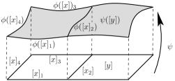
Figure 2: A discrete field $\phi$ and its associated mapping $\psi:\mathbb{X}^{k}\rightarrow\mathbb{G}^{k}$

Proposition 3.8.

There is a one-to-one correspondence between groupoid morphisms $\phi:V\times V\rightarrow G$ and mappings $\psi:\mathbb{X}^{k}\rightarrow\mathbb{G}^{k}$ satisfying the morphism property.

Proof:  We have already associated with a groupoid morphism $\phi$ a map $\psi$ satisfying the morphism property. To prove the converse, let $\psi:\mathbb{X}^{k}\rightarrow\mathbb{G}^{k}$ be a map satisfying the morphism property. Define first $\phi:E\rightarrow G$ as follows.

1. For $(u,u)\in E$, we take a $k$-gon $[x]$ having $u$ as its $l$th vertex: $u=\alpha_{X}([x]_{l})$ and we put

   $$\phi(u,u)=\alpha^{(l)}(\psi([x])).$$

   It is straightforward but rather tedious to show that this expression does not depend on the choice of $[x]$. Let $[y]$ be another $k$-gon, with $u$ as its $m$th vertex. Let us assume for the sake of simplicity that $u$ has degree four (the general case can be dealt with by repeated application of this special case). Then the edges that emerge from $u$ are $[x]_{l}$ and $[y]_{m}$, as well as $([x]_{l-1})^{-1}$ and $([y]_{m-1})^{-1}$ (see figure 3) and there exists exactly one $k$-gon $[z]$ such that

   $$[z]_{n}=([x]_{l})^{-1}\quad\mathrm{and}\quad[z]_{n+1}=([y]_{m-1})^{-1}.$$

   By definition, we have that $\beta(\psi([z])_{n})=\alpha(\psi([z])_{n+1})$ and $\beta(\psi([y])_{m-1})=\alpha(\psi([y])_{m})$. On the other hand, the morphism property ensures that

   $$\psi([x])_{l}=(\psi([z])_{n})^{-1}\quad\mathrm{and}\quad\psi([y])_{m-1}=(\psi([z])_{n+1})^{-1}.$$

   By applying $\alpha$ to the left equality and $\beta$ to the right equality, we finally obtain that

   $$\alpha^{(l)}(\psi([x]))=\alpha^{(m)}(\psi([y])),$$

   which shows that $\phi(u,u)$ does not depend on $[x]$.

   

   Figure 3: A vertex of degree four.

2. For $(u,v)\in E$, $u\neq v$, we take $[x]$ in $\mathbb{X}^{k}$ such that $(u,v)=[x]_{l}$ and we put

   $$\phi(u,v)=\psi([x])_{l}.$$

   This is well defined because of the morphism property and, moreover, $\phi$ satisfies $\phi(y,x)=(\phi(x,y))^{-1}$.

By applying proposition 3.6 we obtain the desired morphism $\phi:V\times V\rightarrow G$. $\Box$

Note that we can still view the developments in the preceding sections as follows. First, the frame bundle of $X$ was discretized by considering the set of $k$-gons $\mathbb{X}^{k}$. Secondly, the jet bundle was discretized by essentially the same procedure: as a jet in the continuous case can be identified with a “horizontal” subspace, we discretised the jet bundle of $\pi$ by approximating jets by $k$-gons in $G$. Finally, we introduced discrete fields as groupoid morphisms from $V\times V$ to $G$, or, equivalently, mappings from $\mathbb{X}^{k}$ to $\mathbb{G}^{k}$ satisfying the morphism property. This property can be seen as the discrete analogue of a section of $J^{1}\pi$ being holonomic.

Remark 3.9.

It is perhaps useful to illustrate the theory developed so far by applying it to groupoid mechanics. In this case, the base space $X$ is $\mathbb{R}$, but all of the constructions for $X=\mathbb{R}^{2}$ carry through to this case. As a discretization of $\mathbb{R}$, we choose the canonical injection $i:\mathbb{Z}\hookrightarrow\mathbb{R}$. A discrete field can then be identified with a bi-infinite sequence of pairwise composable groupoid elements $\ldots,g_{-2},g_{-1},g_{0},g_{1},\ldots$, which is precisely the definition of an admissible sequence in [24, 35]. $\diamond$

3.5 The prolongation $P^{k}\mathbb{G}$

We recall that the discrete jet bundle $\mathbb{G}^{k}$ is equipped with $k$ generalized source maps defined as $\alpha^{(i)}([g])=\alpha([g]_{i})$. By use of these maps, we define the prolongation $P^{k}\mathbb{G}$ of $\mathbb{G}^{k}$ through the following commutative diagram:

Hence, $P^{k}\mathbb{G}$ consists of elements $([g];v_{1},\ldots,v_{k})$, where $v_{i}\in A_{\alpha(g_{i})}G$ for each $i=1,\ldots,k$. We denote by $\pi^{(k)}:P^{k}\mathbb{G}\rightarrow\mathbb{G}^{k}$ the projection which maps $([g];v_{1},\ldots,v_{k})$ onto $[g]$. Furthermore, there exist $k$ bundle morphisms $(P^{(i)},p^{(i)}):P^{k}\mathbb{G}\rightarrow PG$, defined as follows. The base space map $p^{(i)}:\mathbb{G}^{k}\rightarrow G$ is the projection onto the $i$th factor, $p^{(i)}([g])=[g]_{i}$, and the total space map $P^{(i)}$ is defined as

$$P^{(i)}([g];v_{1},\ldots,v_{k})=(g_{i};v_{i},v_{i+1}).$$

The definition of $P^{k}\mathbb{G}$ is strongly reminiscent of that of the prolongation of a Lie groupoid over a fibration (see section 2.4), although in general $\mathbb{G}^{k}$ is not a groupoid. The exact nature of $P^{k}\mathbb{G}$ is unclear at this stage, but we will show (see theorem 3.13) that the algebroid structure of $PG$ can be used to equip $P^{k}\mathbb{G}$ with a Lie algebroid structure by demanding that the maps $(P^{(i)},p^{(i)})$ are Lie-algebroid morphisms.

Remark 3.10.

For $k=2$, the manifold $\mathbb{G}^{2}$ is diffeomorphic to $G$, with the diffeomorphism $\varphi$ mapping each pair $(g,g^{-1})$ onto $g$. Note that $p^{(1)}=\varphi$. In addition, we have that

$$\alpha^{(1)}=\alpha\circ\varphi\quad\mathrm{and}\quad\alpha^{(2)}=\beta\circ\varphi,$$

confirming our intuition that the maps $\alpha^{(i)}$ are some sort of “generalized source maps”. Furthermore, the projection $P^{(1)}$ is given by

$$P^{(1)}(g,g^{-1};u_{\alpha(g)},v_{\beta(g)})=(g;u_{\alpha(g)},v_{\beta(g)}),$$

and so in fact it is just the natural identification of $P^{2}\mathbb{G}$ with $PG$. On the other hand, $P^{(2)}$ is given by

$$P^{(2)}(g,g^{-1};u_{\alpha(g)},v_{\beta(g)})=(g^{-1};v_{\beta(g)},u_{\alpha(g)}).$$

We recalled in section 2.4 that $PG$ is a groupoid over $AG$ in a natural way. A brief comparison shows that $P^{(2)}$ is just the inversion mapping of $PG$, once we use $P^{(1)}$ to identify $PG$ and $P^{2}\mathbb{G}$. $\diamond$

3.5.1 The injection $\mathcal{I}:P^{k}\mathbb{G}\hookrightarrow T\mathbb{G}^{k}$

Of central importance for the following developments is the fact that there exists a bundle injection $\mathcal{I}$ of $P^{k}\mathbb{G}$ into $T\mathbb{G}^{k}$. In order to define $\mathcal{I}$, we recall that a section $v$ of the Lie algebroid $AG$ defines on $G$ a left-invariant vector field $v^{L}$ and a right-invariant vector field $v^{R}$ (see expression (1)). We also recall that we use the same notation for the pointwise operation (see remark 2.1).

Now, let $([g];v_{1},\ldots,v_{k})$ be any element of $P^{k}\mathbb{G}$, and define $\mathcal{I}([g];v_{1},\ldots,v_{k})\in T_{[g]}\mathbb{G}^{k}$ as

$$\mathcal{I}([g];v_{1},\ldots,v_{k})=(v_{1}^{R}(g_{1})+v_{2}^{L}(g_{1}),v_{2}^{R}(g_{2})+v_{3}^{L}(g_{2}),\ldots,v_{k}^{R}(g_{k})+v_{1}^{L}(g_{k})).$$

To prove that the right-hand side is a tangent vector to $\mathbb{G}^{k}$ at $[g]$, we take for each $i=1,\ldots,k$ a curve $t\mapsto h_{i}(t)\in\mathcal{F}^{\alpha}(g_{i})$ in the $\alpha$-fibre through $g_{i}$ such that $h_{i}(0)=\alpha(g_{i})$ and $\dot{h}_{i}(0)=v_{i}$. Then the vector on the right-hand side is the tangent vector at $0$ to the following curve in $\mathbb{G}^{k}$:

$$t\mapsto\big{(}h_{1}^{-1}(t)g_{1}h_{2}(t),h_{2}^{-1}(t)g_{2}h_{3}(t),\ldots,h_{k}^{-1}(t)g_{k}h_{1}(t)\big{)}.$$

Definition 3.11.

Let $[g]$ be an element of $\mathbb{G}^{k}$. The $i$th tangent lift is the map $L^{(i)}_{[g]}:A_{\alpha(g_{i})}G\rightarrow T_{[g]}\mathbb{G}^{k}$ defined as

$$L^{(i)}_{[g]}(v)=\mathcal{I}([g];0,\ldots,0,v,0,\ldots,0)\quad\text{for }v\in A_{\alpha(g_{i})}G,$$

where $v$ occupies the $i$th position among the arguments of $\mathcal{I}([g];\ldots)$. We will frequently use the notation $v^{(i)}_{[g]}$ for the element $L^{(i)}_{[g]}(v)$.

Remark 3.12.

We pointed out that $P^{2}\mathbb{G}$ is isomorphic to $PG$. In this case, the injection $\mathcal{I}$ is given by

$$\mathcal{I}:(g;u_{\alpha(g)},v_{\beta(g)})\mapsto T(r_{g}\circ i)(u_{\alpha(g)})+Tl_{g}(v_{\beta(g)})\in V_{g}\beta\oplus V_{g}\alpha,$$

and coincides with the isomorphism $\Theta:PG\rightarrow V\beta\oplus V\alpha$ (see section 2.4). In this case, the map $\mathcal{I}$ can also be seen as the anchor of the Lie algebroid $PG$. This theme will return in the next section, when we endow $P^{k}\mathbb{G}$ with the structure of a Lie algebroid, with $\mathcal{I}$ as its anchor map. $\diamond$

3.5.2 The Lie algebroid structure on $\pi^{(k)}:P^{k}\mathbb{G}\rightarrow\mathbb{G}^{k}$

In order to endow $P^{k}\mathbb{G}$ with the structure of a Lie algebroid, we introduce the concept of the lift of a section of $PG$ to $P^{k}\mathbb{G}$, not to be confused with the tangent lift of definition 3.11 (In fact, the lift operation defined here will be used only in this section).

We recall that a pair of sections $u,v$ of $AG$ induces a section $X$ of $PG\rightarrow G$ according to $X(g)=(g;u_{\alpha(g)},v_{\beta(g)})$. The Lie bracket on $PG$ is completely determined by its action on sections of this form (see section 2.4.1). We now define the $i$th lift of $X$ as the section $X_{(i)}$ of $P^{k}\mathbb{G}$ constructed as follows:

$$X_{(i)}([g])=([g];0,\ldots,0,\underbrace{u_{\alpha(g_{i})}}_{i},\underbrace{v_{\alpha(g_{i+1})}}_{i+1},0,\ldots,0)\quad\text{for }[g]\in\mathbb{G}^{k}.$$ (9)

We will show that $P^{k}\mathbb{G}$ can be equipped with the structure of a Lie algebroid over $\mathbb{G}^{k}$, and that its Lie bracket is completely determined by its action on sections $X_{(i)}$ of the form (9).

Theorem 3.13.

There exists a unique Lie algebroid structure on $\pi^{(k)}:P^{k}\mathbb{G}\rightarrow\mathbb{G}^{k}$ such that each projection map $P^{(i)}:P^{k}\mathbb{G}\rightarrow PG$ is a morphism of Lie algebroids. This Lie algebroid structure is characterized by

1. the anchor $\rho^{(k)}:P^{k}\mathbb{G}\rightarrow T\mathbb{G}^{k}$ coincides with the injection $\mathcal{I}$ defined in section 3.5.1;

2. for $X,Y\in\mathrm{Sec}(AG)$ and $X_{(i)},Y_{(i)}$ the corresponding $i$th lifts, the bracket of $X_{(i)}$ and $Y_{(i)}$ is determined by

   $$P^{(i)}\circ[X_{(i)},Y_{(i)}]=[X,Y]\circ p^{(i)}.$$ (10)

We denote the associated exterior differential on $\bigwedge(P^{k}\mathbb{G})^{\ast}$ by $\mathrm{d}^{(k)}$.

Proof:  As all of the projection mappings $(P^{(i)},p^{(i)})$ are Lie algebroid morphisms, the anchor $\rho^{(k)}$ of $P^{k}\mathbb{G}$ satisfies

$$\hat{\rho}\circ P^{(i)}=Tp^{(i)}\circ\rho^{(k)},$$

where $\hat{\rho}:PG\rightarrow TG$ is the anchor of $PG$ (see section 2.4.1). Hence, the $i$th component of $\rho^{(k)}([g];v_{1},\ldots,v_{k})$ is just $\rho(g_{i};v_{i},v_{i+1})$, which is equal to $v_{i}^{R}(g_{i})+v_{i+1}^{L}(g_{i})$. We conclude that $\rho^{(k)}$ is precisely the injection $\mathcal{I}$.

The $i$th lift $X_{(i)}$ of $X$ satisfies

$$P^{(i)}\circ X_{(i)}=X\circ p^{(i)}$$ (11)

and the bracket of $X_{(i)}$ and $Y_{(i)}$ is therefore given by the corresponding expression in (10). This follows from [20, def. 1.3] by noting that (11) is the $P^{(i)}$-decomposition of $X_{(i)}$. It is easy to see that the bracket of two $i$th lifts is uniquely determined by (10). That the bracket of two arbitrary sections of $\pi^{(k)}$ is also determined by this expression, is a consequence of the fact that one may lift a basis $\{e_{\alpha}\}$ of sections of $PG$ to yield a basis $\{(e_{\alpha})_{(i)}\}$ of sections of $\pi^{(k)}$. $\Box$

4 Lagrangian field theories

After the discussion in the previous sections of the geometrical background for our treatment of discrete field theories, we now turn to the fields themselves, as well as the equations that govern their behaviour. These equations will turn out to be (implicit or explicit) difference equations.

The key element in constructing these discrete field equations is the specification of a discrete Lagrangian, i.e. a smooth function $L$ on $\mathbb{G}^{k}$. Associated to such a discrete Lagrangian is an action sum — the discrete counterpart of the action integral in continuous field theory. As we will see, the discrete field equations arise by extremizing (in some suitable sense) this action sum.

Before deriving the discrete field equations, we will first construct some intrinsic objects on the prolongation bundle $\pi^{(k)}:P^{k}\mathbb{G}\rightarrow\mathbb{G}^{k}$ and we will argue that all of these objects have a natural counterpart in continuous field theories. These include, among other things, the Poincaré-Cartan forms and the induced Legendre transformations. In § 5, we will make the link with [26] when we turn our attention to an important special case: that of the pair groupoid $G=Q\times Q$.

4.1 The Poincaré-Cartan forms

Let $L:\mathbb{G}^{k}\rightarrow\mathbb{R}$ be a discrete Lagrangian. To $L$ one can associate $k$ sections $\theta^{(i)}_{L}$ of $(\pi^{(k)})^{\ast}:(P^{k}\mathbb{G})^{\ast}\rightarrow\mathbb{G}^{k}$, called Poincaré-Cartan forms, which are defined as follows:

$$\theta^{(i)}_{L}([g];v_{1},\ldots,v_{k})=(v_{i}^{(i)})_{[g]}(L),$$

where $v_{i}\in A_{\alpha(g_{i})}G$ and $v^{(i)}_{i}$ is the $i$th tangent lift of $v_{i}$ to $\mathbb{G}^{k}$ (cf. definition 3.11). As $\sum v^{(i)}_{i}=\mathcal{I}([g];v_{1},\ldots,v_{k})$, we may conclude that

$$\mathrm{d}^{(k)}L=\sum_{i=1}^{k}\theta^{(i)}_{L}.$$

Remark 4.1.

In the case $k=2$, it follows from remark 3.12 that $\theta^{(1)}_{L}$, resp. $\theta^{(2)}_{L}$, can be identified with the Poincaré-Cartan forms $\theta^{-}_{L}$, resp. $\theta^{+}_{L}$, defined in [24] as

$$\theta^{-}_{L}(g;u_{\alpha(g)},v_{\beta(g)})=\mathrm{d}L(g)(u^{R}(g))\quad\mathrm{and}\quad\theta^{+}_{L}(g;u_{\alpha(g)},v_{\beta(g)})=\mathrm{d}L(g)(v^{L}(g)).$$

Indeed, let us consider the function $L_{\mathrm{mech}}$ on $G$ given by $L_{\mathrm{mech}}=\varphi_{\ast}L$, where $\varphi:\mathbb{G}^{2}\rightarrow G$ is the diffeomorphism introduced in remark 3.10, or, explicitely, $L_{\mathrm{mech}}(g)=L(g,g^{-1})$. Then, by definition,

$$\theta_{L}^{(1)}(g,g^{-1};u_{\alpha(g)},v_{\beta(g)})=\frac{\mathrm{d}}{\mathrm{d}t}L(h^{-1}(t)g,g^{-1}h(t))\Big{|}_{0},$$

where $h(t)\in\mathcal{F}^{\alpha}(g)$ is such that $h(0)=\alpha(g)$ and $\dot{h}(0)=u_{\alpha(g)}$. The right-hand side can now be rewritten as

$$\frac{\mathrm{d}}{\mathrm{d}t}L_{\mathrm{mech}}(h^{-1}(t)g)\Big{|}_{0}=\left<\mathrm{d}L_{\mathrm{mech}},T(r_{g}\circ i)(u_{\alpha(g)})\right>=\theta^{-}_{L}(g;u_{\alpha(g)},v_{\beta(g)}).$$

There is a similar identification of $\theta^{(2)}_{L}$ with $\theta^{+}_{L_{\mathrm{mech}}}$. $\diamond$

4.2 The field equations

We now proceed to derive the discrete field equations for a Lie groupoid morphism $\phi:V\times V\rightarrow G$ by varying a discrete action sum. Let $L:\mathbb{G}^{k}\rightarrow\mathbb{R}$ be a discrete Lagrangian and define the action sum as

$$S(\phi)=\sum_{[x]\in\mathbb{X}^{k}}L(\psi([x])),$$ (12)

where $\psi$ is the map from $\mathbb{X}^{k}$ to $\mathbb{G}^{k}$ associated to the morphism $\phi$ (see proposition 3.8). Strictly speaking, one should take care to ensure that this summation is finite by restricting to morphisms $\phi$ whose domain of definition $U\subset V\times V$ only contains a finite number of edges.

4.2.1 Variations

In this section, we define the concept of a variation, both finite and infinitesimal. A key property is that the variation of a groupoid morphism yields a new groupoid morphism. In order to formalize this, we introduce the concept of morphism properties for mappings from $\mathbb{G}^{k}$ onto itself. These properties are very similar to the morphism property introduced in (8).

Let us introduce a slight modification of the source mappings $\alpha^{(i)}$:

$$\hat{\alpha}^{(i)}:\mathbb{G}^{k}\rightarrow\mathbb{G}^{k},\quad\hat{\alpha}^{(i)}([g])=(\alpha([g]_{i}),\ldots,\alpha([g]_{i})).$$

It is obvious that for any $l\leq k$, $\left(\hat{\alpha}^{(i)}([g])\right)_{l}=\alpha^{(i)}([g])$.

Definition 4.2.

A map $\Psi:\mathbb{G}^{k}\rightarrow\mathbb{G}^{k}$ is said to satisfy the morphism properties if, for all $[g],[h]\in\mathbb{G}^{k}$,

1. $\Psi\circ\hat{\alpha}^{(i)}=\hat{\alpha}^{(i)}\circ\Psi$ for $i=1,\ldots,k$;

2. if $[g]_{l}=[h]_{m}$, then $\Psi([g])_{l}=\Psi([h])_{m}$.

Proposition 4.3.

There is a one-to-one correspondence between groupoid morphisms $\Phi:G\rightarrow G$ and mappings $\Psi:\mathbb{G}^{k}\rightarrow\mathbb{G}^{k}$ satisfying the morphism properties.

Proof:  Let $\Phi$ be a morphism from $G$ to itself. As in (7), $\Phi$ induces a mapping $\Psi:\mathbb{G}^{k}\rightarrow\mathbb{G}^{k}$ satisfying the morphism properties, namely:

$$\Psi([g])=\left(\Phi([g]_{1}),\ldots,\Phi([g]_{k})\right).$$

Conversely, let $\Psi:\mathbb{G}^{k}\rightarrow\mathbb{G}^{k}$ be a mapping satisfying the morphism properties and let $g$ be any element of $G$. In order to define $\Phi(g)$, we take any $[\eta]\in\mathbb{G}^{k}$ such that there exists a natural number $l\leq k$ for which $g=[\eta]_{l}$. We then put

$$\Phi(g):=\Psi([\eta])_{l}.$$

Morphism property II ensures that $\Phi(g)$ depends only on $g$ and not on the other components of $[\eta]$. We now have to check that $\Phi$ is a morphism of $G$ to itself.

1. In order to prove that $\alpha\circ\Phi=\Phi\circ\alpha$, we take any $g\in G$ and consider $[\eta]\in\mathbb{G}^{k}$ such that $[\eta]_{l}=g$. Then $\alpha(\Phi(g))=\alpha(\Psi([\eta])_{l})=\alpha^{(l)}(\Psi([\eta]))$.

   However, because of morphism property I we have

   $$\hat{\alpha}^{(l)}\big{(}\Psi([\eta])\big{)}=\Psi\big{(}\hat{\alpha}^{(l)}([\eta])\big{)}=\Psi\big{(}(\alpha(g),\ldots,\alpha(g))\big{)}.$$ (13)

   For any arbitrary $m\leq k$, we have that $\Phi(\alpha(g))=\Psi\big{(}(\alpha(g),\ldots,\alpha(g))\big{)}_{m}$, and so, by considering the $m$th component of (13),

   $$\Phi(\alpha(g)) =\left(\hat{\alpha}^{(l)}\big{(}\Psi([\eta])\big{)}\right)_{m}$$

   $$=\alpha^{(l)}\big{(}\Psi([\eta])\big{)},$$

   from which we conclude that $\alpha(\Phi(g))=\Phi(\alpha(g))$ for all $g\in G$. A similar argument can be used to show that $\Phi$ commutes with $\beta$.

2. We now show that $\Phi(g^{-1})=\Phi(g)^{-1}$ for any $g\in G$. Let

   $$[\xi]=(g,g^{-1},\alpha(g),\ldots,\alpha(g)),$$

   then $\Psi([\xi])_{1}=\Phi(g)$, $\Psi([\xi])_{2}=\Phi(g^{-1})$ and $\Psi([\xi])_{j}=\Phi(\alpha(g))$ for $j=3,\ldots,k$. Moreover, since $\Psi([\xi])\in\mathbb{G}^{k}$, we have, by definition of $\mathbb{G}^{k}$, that $\Psi([\xi])_{1}\cdots\Psi([\xi])_{k}=\alpha(\Psi([\xi])_{1})$, or

   $$\Phi(g)\Phi(g^{-1})\Phi(\alpha(g))\cdots\Phi(\alpha(g))=\alpha(\Phi(g)),$$

   which, after simplication, leads to $\Phi(g^{-1})=\Phi(g)^{-1}$.

3. Finally, we have to show that if $(g,h)$ is a composable pair, i.e. $\beta(g)=\alpha(h)$, then $(\Phi(g),\Phi(h))$ is also composable, and moreover, $\Phi(gh)=\Phi(g)\Phi(h)$. The proof of this property is similar to the proof of the previous property.

   Consider the following $k$-gon:

   $$[\eta]=(g,h,(gh)^{-1},\alpha(g),\ldots,\alpha(g)).$$

   Then, as $\Psi([\eta])\in\mathbb{G}^{k}$, we conclude that, first of all, $\beta(\Phi(g))=\alpha(\Phi(h))$, and secondly

   $$\Phi(g)\Phi(h)\Phi((gh)^{-1})=\alpha\big{(}\Phi(g)\big{)}.$$

   By using the previous properties, as well as some of the standard properties of the groupoid $G$, we find that $\Phi(gh)=\Phi(g)\Phi(h)$.

We conclude that $\Phi:G\rightarrow G$ is a groupoid morphism. $\Box$

Corollary 4.4.

Let $\Psi:\mathbb{G}^{k}\rightarrow\mathbb{G}^{k}$ be a map satisfying the morphism properties. Then for each $[g]\in\mathbb{G}^{k}$,

$$\Psi([g]^{-1})=\Psi([g])^{-1}.$$

Proof:  This can be proved directly, or by noting that $\Psi$ induces a groupoid morphism $\Phi$ such that

$$\Psi([g])=\big{(}\Phi([g]_{1}),\ldots,\Phi([g]_{k})\big{)},$$

and writing out the definition of $[g]^{-1}$ and $\Psi([g])^{-1}$. $\Box$

After these introductory lemmas, we now turn to the concepts of finite and infinitesimal variations of a morphism $\phi:V\times V\rightarrow G$. Before doing so, we remark that any subset $\hat{U}$ of $\mathbb{X}^{k}$ uniquely determines a subset $U$ of $V\times V$, consisting of all the edges of all faces contained in $\hat{U}$. We then define the boundary $\partial U\subset V\times V$ to be the following set:

$$\partial U:=\big{\{}(u,v)\in V\times V:\text{$\exists[x],[y]\in\mathbb{X}^{k}$ such that $[x]_{l}=(u,v),[y]_{m}=(v,u)$}$$

$$\text{and $[x]\in\hat{U},[y]\notin\hat{U}$}\big{\}}.$$

In other words, the boundary $\partial U$ consists of edges that, when traversed in opposite directions, are part of two $k$-gons $[x]$ and $[y]$, one of which is contained in $\hat{U}$, while the other one is not.

Definition 4.5.

A finite variation over $\hat{U}\subset\mathbb{X}^{k}$ of a morphism $\phi:V\times V\rightarrow G$, with associated mapping $\psi:\mathbb{X}^{k}\rightarrow\mathbb{G}^{k}$, is a map $\Psi:\mathbb{R}\times\psi(\hat{U})\rightarrow\psi(\hat{U})$ such that for each fixed $t\in\mathbb{R}$, $\Psi_{t}:=\Psi(t,\cdot)$ satisfies the morphism properties, and which has the following form: for each $[g]\in\psi(\hat{U})$ there exist maps $h_{i}:\mathbb{R}\rightarrow G$ such that

$$\Psi_{t}([g]):=\Psi(t,[g])=(h_{1}(t)^{-1}g_{1}h_{2}(t),h_{2}(t)^{-1}g_{2}h_{3}(t),\ldots,h_{k}(t)^{-1}g_{k}h_{1}(t)),$$ (14)

where $h_{i}(0)=\alpha(g_{i})$ and $h_{i}(t)\in\mathcal{F}^{\alpha}(g_{i})$. In addition, if $[g]_{l}\in\phi(\partial U)$, then $h_{l}(t)=\alpha([g]_{l})$ and $h_{l+1}(t)=\beta([g]_{l})$ for all $t\in\mathbb{R}$.

Note that $\Psi_{t}$ doesn’t have to be defined on the whole on $\mathbb{G}^{k}$, but only on the image of $\hat{U}$ under $\psi$. Note furthermore that $\Psi_{0}$ is the identity mapping on $\psi(\hat{U})$, since each of the curves $h_{i}:\mathbb{R}\rightarrow G$ in (14) satisfies $h_{i}(0)=\alpha(g_{i})$.

Remark 4.6.

It should be emphasised that in (14), each of the curves $h_{i}:\mathbb{R}\rightarrow\mathcal{F}^{\alpha}(g_{i})$ depends only on $\alpha(g_{i})$, and not on the whole of $[g]$ as might be expected. In order to prove this, consider the morphism $\Phi_{t}$ associated to the variation $\Psi_{t}$ and let $g,g^{\prime}$ be elements of $G$ such that $\beta(g)=\alpha(g^{\prime})$. Then

$$\Phi_{t}(g)=h(t)^{-1}gk(t)\quad\mathrm{and}\quad\Phi_{t}(g^{\prime})=h^{\prime}(t)^{-1}g^{\prime}k^{\prime}(t),$$

which makes it clear that $h(t),k(t)$ can only depend on $g$, and $h^{\prime}(t),k^{\prime}(t)$ only on $g^{\prime}$. However, as $(g,g^{\prime})$ is a composable pair, so is their image under $\Phi_{t}$ and therefore $h^{\prime}(t)=k(t)$. We conclude that $k(t)$ cannot depend on $g$ itself but only on $\alpha(g)$. For the variation (14), a similar argument implies that each $h_{i}$ only depends on $\alpha(g_{i})$. $\diamond$

Remark 4.7.

Let $[x],[y]\in\mathbb{X}^{k}$ be two $k$-gons that have an edge in common, e.g. $[x]_{l}=[y]_{m}^{-1}$ for $l,m\leq k$. Consider now their images under the mapping $\psi$ associated to a morphism $\phi:V\times V\rightarrow G$, namely $[\eta]=\phi([x])$ and $[\xi]=\phi([y])$. Because of the morphism property, we conclude that $[\eta]_{l}=[\xi]_{m}^{-1}$. Moreover, $([\eta]_{l-1},[\xi]_{m+1})$ is a composable pair, as is $([\xi]_{m-1},[\eta]_{l+1})$. Let $\Psi$ be a variation of $\phi$; it is interesting to compare its action on $[\eta]$ and $[\xi]$. Putting

$$\Psi_{t}([\eta])=(\ldots,h_{l-1}(t)^{-1}\eta_{l-1}h_{l}(t),h_{l}(t)^{-1}\eta_{l}h_{l+1}(t),h_{l+1}(t)^{-1}\eta_{l+1}h_{l+2}(t),\ldots),$$

where we denote $[\eta]_{i}$ simply by $\eta_{i}$, $i=1,\ldots,k$, the morphism properties that $\Psi_{t}$ has to satisfy, allow us to conclude that the variation of $[\xi]$ is given by the form

$$\Psi_{t}([\xi])=(\ldots,k_{m-1}(t)^{-1}\xi_{m-1}h_{l+1}(t),h_{l+1}(t)^{-1}\xi_{m}h_{l}(t),h_{l}(t)^{-1}\xi_{m+1}k_{m+2}(t),\ldots).$$

The important thing to note is that a composable pair, for example $([\eta]_{l-1},[\xi]_{m+1})$, is mapped to another composable pair, in this case $(\Psi_{t}([\eta])_{l-1},\Psi_{t}([\xi])_{m+1})$. $\diamond$

In conclusion, although definition 4.5 might seem quite involved at first, it has nevertheless a clear geometric interpretation. Indeed, each edge $g$ in the image of $U$ under the discrete field $\phi$ is varied according to the following prescription: there exist curves $h(t)$ and $k(t)$ in $\mathcal{F}^{\alpha}(g)$, with $h(0)=k(0)=\alpha(g)$ such that the variation of $g$ can be expressed as

$$g\mapsto h(t)^{-1}gk(t).$$

The edges of the boundary $\partial U$ are not varied. Imposing the morphism condition on $\Psi_{t}$ ensures us that each edge is varied in a uniquely determined way, and moreover, composable edges (i.e. having a vertex in common) are mapped to composable edges. We have sketched the effect of a finite variation on a discrete field in figure 4.

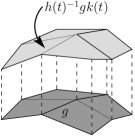
Figure 4: A variation of a discrete field (boundary not shown).

Definition 4.8.

An infinitesimal variation over $\hat{U}\subset\mathbb{X}^{k}$ of a morphism $\phi:V\times V\rightarrow G$ is a section $\Gamma$ of $\pi^{(k)}$, defined on $\psi(\hat{U})$, such that

1. $[g]_{l}=[h]_{m}$ implies that $\Gamma([g])_{l}=\Gamma([h])_{m}$;

2. $[g]_{l}\in\phi(\partial U)$ implies that $\Gamma([g])_{l}=0$,

(with the convention that for $\Gamma([g])=([g];v_{1},\ldots,v_{k})$, $\Gamma([g])_{l}=v_{l}$).

In this definition, the first property ensures that $\Gamma$ attributes a unique Lie algebroid element to each edge, whereas the second property expresses the fact that $\Gamma$ is zero on the image of $\partial U$ under $\phi$. We may therefore conclude that, because of the additional conditions in definition 4.8, an infinitesimal variation can also be interpreted as a section of $PG\rightarrow G$ defined on $\phi(U)$, or equivalently, a section of $\phi^{\ast}PG$ which is zero on $\partial U$.

The infinitesimal variation $\Gamma$ associated to a finite variation $\Psi_{t}$ is generated as follows. For $[g]\in\psi(\hat{U})$, consider the curves $h_{i}:\mathbb{R}\rightarrow G$ (cf. definition 4.5) and put

$$\Gamma([g])=([g];v_{1},\ldots,v_{k}),\quad\mathrm{where}\>v_{i}=\dot{h}_{i}(0).$$

The infinitesimal variation $\Gamma$ will satisfy the required conditions since $\Phi_{t}$ has the morphism properties and leaves the image of $\partial U$ invariant.

Conversely, we may “integrate” an infinitesimal variation $\Gamma$ to yield a finite variation. Let $\gamma$ be the section of $PG$ associated to $\Gamma$, which can be written as $\gamma(g)=(g;u_{\alpha(g)},v_{\beta(g)})$, where $u_{\alpha(g)}\in A_{\alpha(g)}G$ and $v_{\beta(g)}\in A_{\beta(g)}G$. Consider now the left- and right-invariant vector fields $u^{L}$ and $v^{R}$, defined as $u^{L}(g)=(u_{\alpha(g)})^{L}(g)$, and $v^{R}=(v_{\beta(g)})^{R}(g)$. Let $\theta:\mathbb{R}\times G\rightarrow G$ the flow of $u^{L}$, and $\varphi$ the flow of $v^{R}$. We then define a morphism $\Phi_{t}:G\rightarrow G$ by putting $\Phi_{t}(g)=\varphi_{t}(g)g\theta_{t}(g)$. It is easy to check that this composition is well defined. Now, the morphism $\Phi_{t}$ induces a finite variation in the sense of definition 4.5 and by construction the associated infinitesimal variation is equal to the original section $\Gamma$.

4.2.2 The field equations

For the sake of clarity, we will derive the field equations in the case where $X(=\mathbb{R}^{2})$ is covered by a quadrangular mesh as in figure 1. This is also one of the cases covered in [26]. The generalization of the field equations to non-regular meshes is straightforward but involves a lot of notational intricacies.

Let $\phi:V\times V\rightarrow G$ be a discrete field, with associated mapping $\psi:\mathbb{X}^{k}\rightarrow\mathbb{G}^{k}$. Consider a finite subset $\hat{U}$ of $\mathbb{X}^{k}$ with its induced set $U\subset V\times V$, and let $\Psi_{t}$ be a finite variation (according to definition 4.5) over $\hat{U}$ of $\phi$. We denote the composition $\Psi_{t}\circ\psi$ as $\psi_{t}$. Because $\Psi_{t}$ satisfies the morphism properties, $\psi_{t}$ induces in turn a groupoid morphism $\phi_{t}:V\times V\rightarrow G$. Note that $\phi_{0}=\phi$.

We now express that the (restricted) morphism $\phi:(V\times V)\cap U\rightarrow G$ extremizes the action sum (12), i.e.

$$\frac{\mathrm{d}}{\mathrm{d}t}S(\phi_{t})\Big{|}_{t=0}=0$$ (15)

for an arbitrary variation $\Psi_{t}$.

Let $u$ be a vertex in $V$; naturally, $u$ is a common vertex of four quadrangles, denoted by $[x]$, $[\hat{x}]$, $[\tilde{x}]$ and $[\check{x}]$. Let us denote by $[g]$, $[\hat{g}]$, $[\tilde{g}]$ and $[\check{g}]$ their corresponding images under $\psi$ (see figure 5 for a schematic representation of these four quadrangles). We will focus on the variation of the image of the center vertex $u$.

Figure 5: Schematic representation of $[g]$, $[\hat{g}]$, $[\tilde{g}]$, and $[\check{g}]$.

The variation $\Psi_{t}$ will map $[g]$ into a new quadrangle $[g^{\prime}]$ of the following form:

$$[g^{\prime}]=(h_{1}^{-1}(t)g_{1}h_{2}(t),h_{2}^{-1}(t)g_{2}h_{3}(t),h^{-1}_{3}(t)g_{3}h_{4}(t),h_{4}^{-1}(t)g_{4}h_{1}(t)),$$ (16)

and likewise for $[\hat{g}]$, $[\tilde{g}]$ and $[\check{g}]$. However, the latter three each have a vertex in common with $[g]$, and because of morphism property II, their variations will be related, as we pointed out in remark 4.7. More precisely, let us focus on the effects of $h_{3}(t)$: the terms in the action sum involving $h_{3}(t)$ are spelled out below:

$$S(\phi_{t})=\cdots +L(h_{1}^{-1}(t)g_{1}h_{2}(t),h_{2}^{-1}(t)g_{2}h_{3}(t),h_{3}^{-1}(t)g_{3}h_{4}(t),h_{4}^{-1}(t)g_{4}h_{1}(t))$$

$$+L(h_{2}(t)\hat{g}_{1}k_{1}(t),k_{1}^{-1}(t)\hat{g}_{2}k_{3}(t),k_{3}^{-1}(t)\hat{g}_{3}h_{3}(t),h_{3}^{-1}(t)g_{4}h_{2}(t))$$

$$+L(h_{3}^{-1}(t)\tilde{g}_{1}k_{3}(t),k_{3}^{-1}(t)\tilde{g}_{2}l_{3}(t),l_{3}^{-1}(t)\tilde{g}_{3}l_{4}(t),l_{4}^{-1}(t)\tilde{g}_{4}h_{3}(t))$$

$$+L(h_{4}^{-1}(t)\check{g}_{1}h_{3}(t),h_{3}^{-1}(t)\check{g}_{2}l_{4}(t),l_{4}^{-1}(t)\check{g}_{3}m_{4}(t),m_{4}^{-1}(t)\check{g}_{4}h_{4}(t)),$$

where $h_{1}(t),h_{2}(t),h_{3}(t),h_{4}(t)$ as well as $k_{2}(t),k_{3}(t)$, $l_{3}(t),l_{4}(t)$ and $m_{4}(t)$ are determined as in def. 4.5.

It is helpful to keep in mind the following relations:

$$g_{2}=\hat{g}_{4}^{-1},\quad\hat{g}_{3}=\tilde{g}_{1}^{-1}\quad\tilde{g}_{4}=\check{g}_{2}^{-1}\quad\mathrm{and}\quad\check{g}_{1}=g_{3}^{-1},$$

expressing the fact that each of the four $k$-gons $[g],[\hat{g}],[\tilde{g}],[\check{g}]$ has an edge in common with two of the other $k$-gons.

By demanding that $S$ be stationary, we obtain

$$v^{(3)}_{[g]}(L)+v^{(4)}_{[\hat{g}]}(L)+v^{(1)}_{[\tilde{g}]}(L)+v^{(2)}_{[\check{g}]}(L)=0,$$

where $v\in AG$ is given by $v=\dot{h}_{3}(0)$, and the superscript $i$ denotes the $i$th tangent lift of an element of $AG$ to $T\mathbb{G}^{k}$ (see definition 3.11).

In conclusion, we have the following characterization of extremals of the action sum (12).

Theorem 4.9.

Let $\phi:V\times V\rightarrow G$ be a groupoid morphism. For any $u\in V$, consider the vertex $\alpha(g)=\phi(u,u)$ and let $[g]$, $[\hat{g}]$, $[\tilde{g}]$ and $[\check{g}]$ be the four quadrangles having the vertex $\alpha(g)$ in common (as in figure 5).

Then $\phi$ is an extremum of the action sum (12) if and only if, for each such vertex $\alpha(g)$ with associated quadrangles $[g]$, $[\hat{g}]$, $[\tilde{g}]$ and $[\check{g}]$, and for each $v\in A_{\alpha(g)}G$, the following holds:

$$v^{(1)}_{[\tilde{g}]}(L)+v^{(2)}_{[\check{g}]}(L)+v^{(3)}_{[g]}(L)+v^{(4)}_{[\hat{g}]}(L)=0.$$ (17)

We refer to the expressions in (17) as the discrete field equations. In the case where $G$ is the pair groupoid, these equations become (implicit or explicit) difference equations (see [26]). We will return to this case in section 5.1.

4.3 The Legendre transformation

In this section, we introduce a notion of Legendre transformation and use it to show that the pullback of the canonical section of a suitable dual bundle yields the Poincaré-Cartan forms constructed in section 4.1. More precisely, the Legendre transformation will be a collection of $k$ bundle maps from $P^{k}\mathbb{G}$ to the bundle $P^{\tau^{\ast}}(AG)\rightarrow A^{\ast}G$. As sketched in section 2.5.1, the dual of the latter is equipped with a canonical section $\theta$ and the pullback of this section by each of the bundle maps corresponding to the Legendre transformation, will provide the full set of Poincaré-Cartan forms.

We first introduce the pullback bundles $P^{(i)}(AG)$, $i=1,\ldots,k$, constructed by means of the following commutative diagram:

The bundles $P^{(i)}(AG)$ bear the same relation to $\mathbb{G}^{k}$ as $P^{\alpha}(AG)$ and $P^{\beta}(AG)$ to $G$.

4.3.1 The mappings $\mathfrak{P}^{(i)}:P^{k}\mathbb{G}\rightarrow P^{(i)}(AG)$

For each $i=1,\ldots,k$, there is a natural injection $\varphi^{(i)}:G\rightarrow\mathbb{G}^{k}$ defined as

$$\varphi^{(i)}(g)=(\alpha(g),\ldots,\alpha(g),g,g^{-1},\alpha(g),\ldots,\alpha(g))$$

where $g$ and $g^{-1}$ occupy the $i$th and the $(i+1)$th position, respectively.

The projections $P^{(i)}:P^{k}\mathbb{G}\rightarrow PG$, as defined in section 3.5, can be used to define projection mappings $\mathfrak{P}^{(i)}:P^{k}\mathbb{G}\rightarrow P^{(i)}(AG)$ by means of the composition

$$\mathfrak{P}^{(i)}:P^{k}\mathbb{G}\stackrel{{\scriptstyle P^{(i)}}}{{\longrightarrow}}PG\stackrel{{\scriptstyle A(\Phi^{\alpha})}}{{\longrightarrow}}P^{\alpha}(AG)\stackrel{{\scriptstyle\mathrm{id}\times T\varphi^{(i)}}}{{\longrightarrow}}P^{(i)}(AG),$$

where $A(\Phi^{\alpha}):PG\rightarrow P^{\alpha}(AG)$ was defined in section 2.5.2.

Remark 4.10.

For $k=2$, we now show that the projections $\mathfrak{P}^{(1)}$ and $\mathfrak{P}^{(2)}$ can be identified with $A(\Phi^{\alpha})$ and $A(\Phi^{\beta})$, respectively. We recall that $P^{2}\mathbb{G}$ is isomorphic to $PG$ and that there is a diffeomorphism $\varphi:\mathbb{G}^{2}\rightarrow G$ sending each $(g,g^{-1})$ to $g$ (see remark 3.10). Hence, $\varphi^{(1)}$ is just $\varphi^{-1}$ and $\varphi^{(2)}$ equals $\varphi^{-1}\circ i$.

There is a natural identification of $P^{(1)}(AG)$ with $P^{\alpha}(AG)$, and of $P^{(2)}(AG)$ with $P^{\beta}(AG)$. Using these identifications, it is straightforward to see that $\mathfrak{P}^{(1)}$ can be identified with $A(\Phi^{\alpha})$. The identification of $\mathfrak{P}^{(2)}$ with $A(\Phi^{\beta})$ takes some more work. Consider first the composition

$$P^{\alpha}(AG)\stackrel{{\scriptstyle\mathrm{id}\times T\varphi^{(2)}}}{{\longrightarrow}}P^{(2)}(AG)\cong P^{\beta}(AG),$$

which is easily seen to be equal to $\mathrm{id}\times Ti$. We then obtain the following for the map $\mathfrak{P}^{(2)}$, considered as a map into $P^{\beta}(AG)$:

$$\left((\mathrm{id}\times Ti)\circ A(\Phi^{\alpha})\circ P^{(2)}\right) (g,g^{-1};u_{\alpha(g)},v_{\beta(g)})$$

$$=(\mathrm{id}\times Ti\circ A(\Phi^{\alpha}))(g^{-1};v_{\beta(g)},u_{\alpha(g)})$$

$$=(\mathrm{id}\times Ti)(v_{\beta(g)},T(r_{g^{-1}}\circ i)(v_{\beta(g)})+Tl_{g^{-1}}(u_{\alpha(g)}))$$

$$=(v_{\beta(g)},T(r_{g}\circ i)(u_{\alpha(g)})+Tl_{g}(v_{\beta(g)}))$$

$$=A(\Phi^{\beta})(g;u_{\alpha(g)},v_{\beta(g)}),$$

where we again refer to section 2.5.2 for the definition of $A(\Phi^{\beta})$. $\diamond$

4.3.2 Definition of the Legendre transformations

Given a Lagrangian $L:\mathbb{G}^{k}\rightarrow\mathbb{R}$, there are $k$ distinguished bundle maps $(P\mathbb{F}L^{(i)},\mathbb{F}L^{(i)})$ from $P^{k}\mathbb{G}$ to the bundle $P^{\tau^{\ast}}(AG)\rightarrow A^{\ast}G$, which we will call Legendre transformations.

For each $i=1,\ldots,k$, the base map $\mathbb{F}L^{(i)}:\mathbb{G}^{k}\rightarrow A^{\ast}G$ is defined as follows. For each $[g]\in\mathbb{G}^{k}$, $\mathbb{F}L^{(i)}([g])$ is the element of $A^{\ast}_{\alpha(g_{i})}G$ defined by

$$\mathbb{F}L^{(i)}([g])(v_{\alpha(g_{i})})=v^{(i)}_{\alpha(g_{i})}(L)\quad\text{for all}\>v_{\alpha(g_{i})}\in A_{\alpha(g_{i})}G.$$

Recall that $v^{(i)}_{\alpha(g_{i})}$ is the $i$th tangent lift of $v_{\alpha(g_{i})}$ to $T_{[g]}\mathbb{G}^{k}$. The total space map $P\mathbb{F}L^{(i)}:P^{k}\mathbb{G}\rightarrow P^{\tau^{\ast}}(AG)$ is defined as the composition $(\mathrm{id}\times T\mathbb{F}L^{(i)})\times\mathfrak{P}^{(i)}$.

Proposition 4.11.

Let $\theta$ be the canonical section of $[P^{\tau^{\ast}}(AG)]^{\ast}\rightarrow A^{\ast}G$ defined in section 2.5.1. Then, for $i=1,\ldots,k$,

$$(P\mathbb{F}L^{(i)},\mathbb{F}L^{(i)})^{\star}\theta=\theta^{(i)}_{L}.$$

Proof:  Let $([g];v_{1},\ldots,v_{k})$ be an element of $P^{k}\mathbb{G}$ and consider

$$[(P\mathbb{F}L^{(i)},\mathbb{F}L^{(i)})^{\star}\theta]_{[g]}([g];v_{1},\ldots,v_{k})=\theta_{\mathbb{F}L^{(i)}([g])}(P\mathbb{F}L^{(i)}([g];v_{1},\ldots,v_{k})).$$ (18)

Now, the canonical section $\theta$ is defined by the following rule: for $\alpha\in A^{\ast}G$ and $(v,X_{\alpha})$ in $(P^{\tau^{\ast}}(AG))_{\alpha}$, we have that $\theta_{\alpha}(v,X_{\alpha})=\alpha(v)$. Noting that

$$P\mathbb{F}L^{(i)}([g];v_{1},\ldots,v_{k})=(v_{i},\cdot)$$

(the precise form of the second argument doesn’t matter), the right-hand side of (18) then becomes

$$\mathbb{F}L^{(i)}([g])(v_{i})=\theta^{(i)}_{L}([g];v_{1},\ldots,v_{k}),$$

where the last equality follows by comparing the definition of the $i$th Poincaré-Cartan form with the $i$th Legendre transformation. $\Box$

4.4 Variational interpretation of the Poincaré-Cartan forms

In this section, we closely follow some of the ideas set out by Marsden, Patrick, and Shkoller in [26]. In that paper, the authors gave a variational definition of discrete multisymplectic field theories. As we pointed out before, the class of field theories that they consider corresponds to the case where the groupoid $G$ over the standard fibre $Q$ is the pair groupoid $Q\times Q$ (see section 5.1).

We now intend to redo their analysis to prove that the Poincaré-Cartan forms that we defined in section 4.1, also arise when considering variations of a morphism $\phi$ over a set $\hat{U}$ such that the boundary $\partial U$ is not fixed. Moreover, we use these observations to derive a criterion of multisymplecticity, and show that the field equations (see theorem 4.9) are multisymplectic in that sense. Again, this is just an extension to the case of an arbitrary groupoid $G$ of the definitions in [26].

4.4.1 Arbitrary variations

Consider a finite subset $\hat{U}$ of $\mathbb{X}^{k}$ with associated boundary $\partial U$. Now, let $\phi:V\times V$ be a morphism and consider a finite variation $\Psi:\mathbb{R}\times\psi(\hat{U})\rightarrow\psi(\hat{U})$ of $\phi$ over $\hat{U}$ as in definition 4.5. However, we now also allow nontrivial variations of the field on the boundary $\partial U$.

When extremizing the action sum (12), there is now a contribution from the interior of $U$, as well as a contribution from the boundary $\partial U$, which takes the following form (with the notations of section 4.2):

$$\frac{\mathrm{d}}{\mathrm{d}t}S(\phi_{t})\Big{|}_{t=0}=\sum_{[x]\cap\partial U\neq\varnothing}\left(\sum_{l;[x]_{l}\in\partial U}\Big{(}\theta^{(l)}_{L}(\psi([x]))\cdot\Gamma_{\psi([x])}\Big{)}\right),$$

where $\Gamma$ is the infinitesimal variation associated to $\Psi$. Once again, we see how the Poincaré-Cartan forms arise naturally in the context of discrete Lagrangian field theories.

4.4.2 Multisymplecticity

By exactly the same reasoning as in [26], we obtain a concise criterion for multisymplecticity. We will not repeat the entire proof, but we only highlight some of the key points. For more information, the reader is referred to [26].

Let us consider, first of all, the set $\mathcal{M}$ of morphisms $\phi:V\times V\rightarrow G$ that solve the discrete field equations. We also assume that $\mathcal{M}$ can be given the structure of a smooth, infinite-dimensional manifold. Then, a first variation of an element $\phi$ of $\mathcal{M}$ is a section $\Gamma$ of $P^{k}\mathbb{G}$ such that the associated finite variation transforms $\phi$ into new solutions of the discrete field equations. As the action sum $S$ can be interpreted as a function on the set of morphisms from $V\times V$ to $G$, and hence defines by restriction a function (also denoted by $S$) on the set $\mathcal{M}$.

By an argument similar to [26, thm. 4.1], it can then be shown that, for any $\phi\in\mathcal{M}$ and $\Gamma_{1},\Gamma_{2}$ first variations of $\phi$, the trivial identity $\mathrm{d}^{2}S(\phi)(\Gamma_{1},\Gamma_{2})\equiv 0$ can equivalently be written as

$$0=\sum_{[x]\cap\partial U\neq\varnothing}\left(\sum_{l;[x]_{l}\in\partial U}\Big{(}\Omega^{(l)}_{L}(\psi([x]))(\Gamma_{1},\Gamma_{2})\Big{)}\right).$$

This characterization of multisymplecticity involves only the quadrangles $[x]$ that contain edges which are part of the boundary $\partial U$.

5 Examples

5.1 The pair groupoid $G=Q\times Q$

In this section, we treat in detail the case where $G$ is the pair groupoid $Q\times Q$. The results we obtain in this case agree with those in [26], which serves as a justification for our approach.

In this case, it is easy to see that $\mathbb{G}^{k}$ is just $Q^{k}$: the identification is given by

$$\big{(}(q_{k},q_{1}),(q_{1},q_{2}),\ldots,(q_{k-1},q_{k})\big{)}\mapsto(q_{1},q_{2},\ldots,q_{k}).$$

Furthermore, the prolongation algebroid $P^{k}\mathbb{G}$ can be identified with the $k$-fold Cartesian product of $TQ$ with itself. For a vector field $v$ on $Q$, the $i$th tangent lift of $v$ is the following section of $(TQ)^{k}$:

$$v^{(i)}:(q_{1},q_{2},\ldots,q_{k})\mapsto(0,\ldots,0,v(q_{i}),0,\ldots,0),$$

where $v(q_{i})$ occupies the $i$th place.

Now, let $L:\mathbb{G}^{k}\rightarrow\mathbb{R}$ be a Lagrangian and denote by $\hat{L}$ the induced map on $Q^{k}$. Then the $i$th Poincaré-Cartan form is defined as

$$\theta^{(i)}_{L}(q_{1},\ldots,q_{k};v_{1},\ldots,v_{k})=\mathrm{d}\hat{L}(q_{1},\ldots,q_{i-1},\cdot,q_{i+1},\ldots,q_{k})\cdot v_{i},$$

where $v_{i}\in T_{q_{i}}Q$ for $i=1,\ldots,k$. This was the original definition of the Poincaré-Cartan forms in [26].

It is instructive to see what becomes of the concepts of finite and infinitesimal variations in this case: an infinitesimal variation is just a vector field on $Q$, whereas a finite variation is the flow of such a vector field.

As we pointed out before, a morphism $\phi:V\times V\rightarrow Q\times Q$ can be seen as an assigment of an element of $Q$ to each vertex in $V$. For the case of the square mesh of figure 1, we may therefore describe the field by assigning a value $\phi_{i,j}\in Q$ to each vertex $(i,j)$. Let $\hat{L}(q_{1},q_{2},q_{3},q_{4})$ be a Lagrangian density; then $\{\phi_{i,j}\}$ is a solution of the field equations (17) associated to $L$ if and only if, for all $(i,j)\in V$,

$$\frac{\partial L}{\partial q_{1}}(\phi_{i,j},\phi_{i+1,j},\phi_{i+1,j+1},\phi_{i,j+1})+\frac{\partial L}{\partial q_{2}}(\phi_{i-1,j},\phi_{i,j},\phi_{i,j+1},\phi_{i-1,j+1})+$$

$$\frac{\partial L}{\partial q_{3}}(\phi_{i-1,j-1},\phi_{i,j-1},\phi_{i,j},\phi_{i-1,j})+\frac{\partial L}{\partial q_{4}}(\phi_{i,j-1},\phi_{i+1,j-1},\phi_{i+1,j},\phi_{i,j})=0.$$

These equations were first derived in [26].

5.2 The Lie-Poisson equations

Consider now the case where the standard fibre $Q$ is a point, and the groupoid $G$ a Lie group. We will take a particular triangular mesh in $X=\mathbb{R}^{2}$, constructed as follows. The vertices are the points in $\mathbb{R}^{2}$ with integer coordinates:

$$V=\{(i,j)\in\mathbb{R}^{2}:i,j\in\mathbb{Z}\}.$$

However, instead of first specifying the set of edges, we start from the set of faces, which we define to be

$$F=\{\big{(}(i,j),(i+1,j),(i+1,j+1)\big{)}\in V\times V\times V\}.$$

The set of edges then consists of “horizontal” edges of the form $((i,j),(i+1,j))$, “vertical” edges of the form $((i,j),(i,j+1))$, and “diagonal” edges of the form $((i,j),(i+1,j+1))$. This type of mesh was used in [26] as well. The idea behind it is that, in the appropriate physical setting, the horizontal edges represent the spatial direction, whereas the vertical direction represents the time direction.

Let us now consider a discrete Lagrangian $L:\mathbb{G}^{3}\rightarrow\mathbb{R}$. Note that $\mathbb{G}^{3}$ is diffeomorphic to $G\times G$ by mapping an element $(g_{1},g_{2},g_{3})\in\mathbb{G}^{3}$ to $(g_{1},g_{2})$. We denote the induced Lagrangian by $\hat{L}$, where $\hat{L}(g_{1},g_{2})=L(g_{1},g_{2},g_{3})$. Given the fact that our triangular mesh is different from the ones we used in the body of the text, it is perhaps useful to derive the field equations from scratch. Let $\phi:V\times V\rightarrow G$ be a morphism and consider a variation $\Psi$ of $\phi$ over some finite domain $\hat{U}$ in $\mathbb{G}^{3}$. It is easy to see that, if $[g]=\psi([x])$ is an element of $\mathbb{G}^{3}$, then the effect of $\Psi$ on $[g]$ is as follows:

$$[g]\mapsto(h_{1}(t)^{-1}g_{1}h_{2}(t),h_{2}(t)^{-1}g_{2}h_{3}(t),h_{3}(t)^{-1}g_{3}h_{1}(t)),$$

where $h_{1},h_{2},h_{3}$ are now arbitrary curves in $G$, such that $h_{1}(0)=h_{2}(0)=h_{3}(0)=e$, the unit in $G$.

Let us now focus on the factor $h_{1}(t)$. Following essentially the same reasoning as in remark 4.7, we see that $h_{1}(t)$ appears not only in the variation of $[g]$ but in the variation of two additional triangles $[\hat{g}]=\psi([\hat{x}])$ and $[\tilde{g}]=\psi([\tilde{x}])$ in the image of $\psi$ as well (see figure 6).

The terms in the action sum involving $h_{1}(t)$ are therefore

$$S(\phi_{t})=\cdots +{L}(h_{1}(t)^{-1}g_{1}h_{2}(t),h_{2}(t)^{-1}g_{2}h_{3}(t),h_{3}(t)^{-1}g_{3}h_{1}(t))$$

$$+{L}(k_{1}(t)^{-1}\hat{g}_{1}k_{2}(t),k_{2}(t)^{-1}\hat{g}_{2}h_{1}(t),h_{1}(t)^{-1}\hat{g}_{3}k_{1}(t))$$

$$+{L}(m_{1}(t)^{-1}\tilde{g}_{1}h_{1}(t),h_{1}(t)^{-1}\tilde{g}_{2}m_{2}(t),m_{2}(t)^{-1}\tilde{g}_{3}m_{1}(t))$$

$$+\cdots,$$

where $k_{1}(t),k_{2}(t)$ and $m_{1}(t),m_{2}(t)$ correspond to the effect of $\Psi$ on the other vertices. We now rewrite this in terms of the induced Lagrangian $\hat{L}$ and demand that $\phi$ extremizes the action sum to obtain the following set of discrete field equations:

$$0=\frac{\mathrm{d}}{\mathrm{d}t}S(\phi_{t}) =\mathrm{d}\big{[}\hat{L}(\cdot,g_{3})\circ r_{g_{1}}\circ i\big{]}\cdot v_{1}+\mathrm{d}\big{[}\hat{L}(g_{1},\cdot)\circ l_{g_{3}}\big{]}\cdot v_{1}$$

$$+\mathrm{d}\big{[}\hat{L}(\hat{g}_{1},\cdot)\circ r_{g_{3}}\circ i\big{]}\cdot v_{1}+\mathrm{d}\big{[}\hat{L}(\cdot,\tilde{g}_{3})\circ l_{\tilde{g}_{1}}\big{]}\cdot v_{1},$$

where $v_{1}=\dot{h}_{1}(0)$. As $h_{1}(t)$ is arbitrary, this implies that, for any six elements in the image of $\phi$, distributed as in figure 6, the following discrete field equations must hold:

$$\Big{(}l_{g_{3}}^{\ast}\mathrm{d}\hat{L}(g_{1},\cdot)-r_{\hat{g}_{3}}^{\ast}\mathrm{d}\hat{L}(\hat{g}_{1},\cdot)\Big{)}+\Big{(}l_{\tilde{g}_{1}}^{\ast}\mathrm{d}\hat{L}(\cdot,\tilde{g}_{3})-r_{g_{1}}^{\ast}\mathrm{d}\hat{L}(\cdot,g_{3})\Big{)}=0.$$

In this expression, one can recognise, roughly speaking, two separate discrete Lie-Poisson equations (see [25]), one for the “spatial” direction and one for the “time” direction.

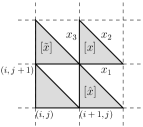
Figure 6: Triangular mesh in $\mathbb{R}^{2}$.

The discrete Lie-Poisson equations arise, among others, in the context of reduction. Let $G$ be a Lie group and consider the pair groupoid $G\times G$ over $G$. Now, if $L:G^{k}\rightarrow\mathbb{R}$ is a discrete Lagrangian, which is left invariant in the sense that $L(gh_{1},gh_{2},gh_{3})=L(h_{1},h_{2},h_{3})$ for all $g,h_{1},h_{2},h_{3}\in G$, and we consider the induced Lagrangian $L^{\prime}:G^{k-1}\rightarrow\mathbb{R}$ defined as

$$L^{\prime}(h_{1}^{-1}h_{2},h_{2}^{-1}h_{3},\ldots,h_{k-1}^{-1}h_{k})=L(h_{1},h_{2},\ldots,h_{k}),$$

then the following holds: a discrete field $\phi:V\times V\rightarrow G$ will solve the field equations for $L$ if its reduced field $\phi:V\times V\rightarrow G$ solves the Lie-Poisson equations. This is proved below in greater generality. Note that one recovers the Lie-Poisson equations by considering the morphism $\Phi:(g,h)\mapsto g^{-1}h$.

Theorem 5.1.

Let $G^{\prime}$ be a Lie groupoid over a manifold $Q^{\prime}$ and consider a morphism $(\Phi,f):(G,Q)\rightarrow(G^{\prime},Q^{\prime})$. Furthermore, let $L^{\prime}:\mathbb{G}^{\prime k}\rightarrow\mathbb{R}$ be a Lagrangian on $\mathbb{G}^{\prime k}$ and consider the induced Lagrangian $L=L^{\prime}\circ\Psi$ on $\mathbb{G}^{k}$, where $\Psi:\mathbb{G}^{k}\rightarrow\mathbb{G}^{\prime k}$ is the map associated to $\Phi$.

A morphism $\phi:V\times V\rightarrow G$ will satisfy the discrete field equations for $L$ if the induced morphism $\Phi\circ\phi:V\times V\rightarrow G^{\prime}$ satisfies the field equations for $L^{\prime}$.

Proof:  The proof relies on the following equality: for $i\leq k$, $[g]\in\mathbb{G}^{k}$, and $v\in A_{x}G$, where $x=\alpha(g_{i})$,

$$v^{(i)}_{[g]}(L)=\left[A\Phi(v)\right]^{(i)}_{\Psi([g])}(L^{\prime}),$$

which is relatively straightforward to prove.

With the same notations as above, this implies that

$$\mathcal{EL}([g],[\hat{g}],[\tilde{g}])\cdot v=\mathcal{EL^{\prime}}(\Psi([g]),\Psi([\hat{g}]),\Psi([\tilde{g}]))\cdot(A\Phi(v)),$$

where we have defined the Euler-Lagrange operator $\mathcal{EL}:\mathbb{G}^{3}\times\mathbb{G}^{3}\times\mathbb{G}^{3}\rightarrow A^{\ast}G$ as

$$\mathcal{EL}([g],[\hat{g}],[\tilde{g}])\cdot v=v^{(1)}_{[g]}(L)+v^{(2)}_{[\tilde{g}]}(L)+v^{(3)}_{[\hat{g}]}(L).$$

Therefore, if $\phi$ is such that $\Phi\circ\phi$ is a solution of the Euler-Lagrange equations for $L^{\prime}$, then $\phi$ itself is a solution of the Euler-Lagrange equations for $L$. $\Box$

Lie-Poisson reduction in discrete field theories is thus very similar to the corresponding theory in mechanics. We glossed over some subtle differences, however, mainly related to the reconstruction problem. This will be treated in more detail in a forthcoming paper.

5.3 Lattice gauge theories and discrete connections

The geometrical setup described in section 3 is very similar to the one used in the treatment of gauge fields on a lattice (see e.g. [19] and the references therein).

Let us consider an arbitrary compact Lie group $G$, which we interpret as a Lie groupoid over a singleton $\{e\}$, with $e$ the unit element of $G$. For definiteness, we assume that the base space $X$ is once again $\mathbb{R}^{2}$ and that a triangulation of $X$ is given.

A discrete gauge field or discrete connection is a map $\psi:E\rightarrow G$, assigning a group element to each edge in $\mathbb{R}^{2}$. The field strength or curvature of such a gauge field is the map $\Omega:F\rightarrow G$ which assigns to each face $f$ the product

$$\Omega(f)=\psi(e_{1})\cdot\psi(e_{2})\cdot\psi(e_{3}),$$

where $e_{1}$, $e_{2}$ and $e_{3}$ are the edges of $f$. Here, we tacitly assume that the edges are oriented and that $\psi(e^{-1})=\psi(e)^{-1}$.

Interpreting the gauge group $G$ as a Lie groupoid over $e$, it is obvious that discrete fields, in the sense of definition 3.5, correspond to flat gauge fields (i.e. gauge fields with vanishing field strength). Indeed, it is precisely the fact that these discrete fields are groupoid morphisms, that makes the field strength vanish.

However, much of our formalism can be extended to the case of arbitrary, non-flat gauge fields. Indeed, let us consider a gauge field $\psi:E\rightarrow G$. In [3], the authors consider a groupoid $\mathcal{P}$, the units of which are the elements of $V$, while the elements of $\mathcal{P}$ are paths in $E$, i.e. sequences of composable elements $e_{1},e_{2},\ldots,e_{m}$ in $E$. A gauge field then gives rise to a morphism $A:\mathcal{P}\rightarrow G$ as follows:

$$A:(e_{1},e_{2},\ldots,e_{m})\mapsto\psi(e_{1})\psi(e_{2})\cdots\psi(e_{m}).$$

If $A$ maps closed loops in $E$ to the unit in $G$, the associated gauge field is flat. In this case, we have the following interesting property: simplicially homotopic paths are mapped to the same element in $G$. This is the discrete version of a well-known property of continuous connections: if $\omega$ is a flat connection, and $\gamma,\gamma^{\prime}$ are closed loops that are homotopic, then the holonomy of $\gamma$ is equal to that of $\gamma^{\prime}$ (see [21, p. 93]). We therefore obtain a morphism $\hat{A}$ from $\hat{\mathcal{P}}$, the groupoid of paths modulo simplicial homotopy, to $G$. In the case where $X=\mathbb{R}^{2}$, $\hat{\mathcal{P}}$ can be identified with $V\times V$, and we are back at our starting point, that of representing flat gauge fields by morphisms from $V\times V$ to $G$.

Remark 5.2.

At first, our use of flat discrete connections might seem to exclude the treatment of gauge theories. A closer look will reveal that the flatness used in the main body of our text plays a similar role as the flatness (or integrability) of the connections used in the connection-theoretic De Donder-Weyl treatment of classical field theories (see [12, 32]) and is hence quite unrelated to the curvature of the fields. $\diamond$

6 Conclusions and outlook

In this paper, we have described a geometric model for discrete field theories. We extended the foundational work done in [26] by allowing for discrete fields that take values in an arbitrary groupoid and we showed that much of the geometric structures from (discrete) field theory, such as the Poincaré-Cartan forms and the notion of multisymplecticity, carry over quite naturally to this setup.

There remain many interesting open problems in this area. In a future publication, we intend to investigate the problem of discrete reduction into further detail, as well as the reconstruction problem. It turns out that, just as in the continuous case (see [13, 14, 15]) there appears an additional condition involving discrete curvature, which is absent from the reconstruction problem in mechanics.

Another interesting link concerns the theory of discrete integrable fields as proposed by Bobenko, Suris, and coworkers (see [1, 7, 6, 4] as well as the references therein). After all, the kind of fields that we investigate here bear some tantalizing resemblances to their zero-curvature representations.

Ultimately, and perhaps not unrelated to the previous point, one would hope that the techniques developed in this paper can be applied to the construction of robust integrators for PDEs. It should be stressed, however, that the concept of “symplectic integrator” for field theories is much more subtle than for simple mechanical systems and that the issue whether multisymplectic integration schemes provide qualitatively better results is usually decided on a case-by-case basis (see for instance [2], where a number of symplectic and multisymplectic schemes are compared in the case of the celebrated Korteweg-de Vries equation).

References

- [1] V. E. Adler, Discrete equations on plane graphs, J. Phys. A: Math. Gen. 34 (2001), 10453–10460.
- [2] U. M. Ascher and R. I. McLachlan, On symplectic and multisymplectic schemes for the KdV equation, To appear in J. Sci. Comput., 2005.
- [3] J. Baez, Quantum Gravity seminar: Gauge Theory and Topology (Week 5, Winter 2005)., Course notes, available from the author’s website http://math.ucr.edu/home/baez/qg-winter2005.
- [4] A. I. Bobenko and U. Pinkall, Discretization of Surfaces and Integrable Systems, Discrete Integrable Geometry and Physics (A. I. Bobenko and R. Seiler, eds.), Oxford University Press, 1999, pp. 3–58.
- [5] A. I. Bobenko and Y. B. Suris, Discrete time Lagrangian mechanics on Lie groups, with an application to the Lagrange top, Comm. Math. Phys. 204 (1999), no. 1, 147–188.
- [6] A. I. Bobenko and Y. B. Suris, Integrable systems on quad-graphs, Int. Math. Res. Not. 11 (2002), 573–611.
- [7] A. I. Bobenko and Y. B. Suris, Discrete differential geometry. Consistency as integrability., Preliminary version of a book, math.DG/0504358.
- [8] T. J. Bridges, Multi-symplectic structures and wave propagation, Math. Proc. Cambridge Philos. Soc. 121 (1997), no. 1, 147–190.
- [9] T. J. Bridges, Canonical multi-symplectic structure on the total exterior algebra bundle, Preprint, 2005.
- [10] T. J. Bridges and G. Derks, Unstable eigenvalues and the linearization about solitary waves and fronts with symmetry, Proc. R. Soc. Lond. A 455 (1999), 2427–2469.
- [11] T. J. Bridges and S. Reich, Multi-symplectic integrators: numerical schemes for Hamiltonian PDEs that conserve symplecticity, Phys. Lett. A 284 (2001), no. 4-5, 184–193.
- [12] J. F. Cariñena, M. Crampin, and L. A. Ibort, On the multisymplectic formalism for first order field theories, Diff. Geom. Appl. 1 (1991), no. 4, 345–374.
- [13] M. Castrillón López, P. L. García Pérez, and T. S. Ratiu, Euler-Poincaré reduction on principal bundles, Lett. Math. Phys. 58 (2001), no. 2, 167–180.
- [14] M. Castrillón López and T. S. Ratiu, Reduction in principal bundles: covariant Lagrange-Poincaré equations, Comm. Math. Phys. 236 (2003), no. 2, 223–250.
- [15] M. Castrillón López, T. S. Ratiu, and S. Shkoller, Reduction in principal fiber bundles: covariant Euler-Poincaré equations, Proc. Amer. Math. Soc. 128 (2000), no. 7, 2155–2164.
- [16] M. Crainic and R. L. Fernandes, Integrability of Lie brackets, Ann. Math. 157 (2003), no. 2, 575–620.
- [17] M. Gotay, J. Isenberg, and J. Marsden, Momentum Maps and Classical Relativistic Fields. Part I: Covariant Field Theory, Preprint, available as physics/9801019.
- [18] C. Günther, The polysymplectic Hamiltonian formalism in field theory and calculus of variations. I. The local case, J. Diff. Geom. 25 (1987), no. 1, 23–53.
- [19] R. Gupta, Introduction to lattice QCD, Course notes, available as hep-lat/9807028.
- [20] P. Higgins and K. Mackenzie, Algebraic constructions in the category of Lie algebroids, J. Algebra 129 (1990), no. 1, 194–230.
- [21] S. Kobayashi and K. Nomizu, Foundations of differential geometry. Vol I, Interscience Publishers, John Wiley & Sons, 1963.
- [22] B. Leimkuhler and S. Reich, Simulating Hamiltonian dynamics, Cambridge Monographs on Applied and Computational Mathematics, vol. 14, Cambridge University Press, Cambridge, 2004.
- [23] K. C. H. Mackenzie, General theory of Lie groupoids and Lie algebroids, London Mathematical Society Lecture Note Series, vol. 213, Cambridge University Press, Cambridge, 2005.
- [24] J. C. Marrero, D. Martín de Diego, and E. Martínez, Discrete Lagrangian and Hamiltonian Mechanics on Lie Groupoids, Available as math.DG/0506299 (2005).
- [25] J. E. Marsden, S. Pekarsky, and S. Shkoller, Discrete Euler-Poincaré and Lie-Poisson equations, Nonlinearity 12 (1999), no. 6, 1647–1662.
- [26] J. E. Marsden, G. W. Patrick, and S. Shkoller, Multisymplectic geometry, variational integrators, and nonlinear PDEs, Comm. Math. Phys. 199 (1998), no. 2, 351–395.
- [27] E. Martínez, Lagrangian mechanics on Lie algebroids, Acta Appl. Math. 67 (2001), no. 3, 295–320.
- [28] E. Martínez, Classical field theory on Lie algebroids: multisymplectic formalism, Preprint, available as math.DG/0411352 (2004).
- [29] E. Martínez, Classical field theory on Lie algebroids: variational aspects, J. Phys. A: Math. Gen. 38 (2005), 7145–7160.
- [30] J. Moser and A. Veselov, Discrete versions of some classical integrable systems and factorization of matrix polynomials, Comm. Math. Phys. 139 (1991), no. 2, 217–243.
- [31] F. Munteanu, A. M. Rey, and M. Salgado, The Günther’s formalism in classical field theory: momentum map and reduction, J. Math. Phys. 45 (2004), no. 5, 1730–1751.
- [32] D. J. Saunders, The Geometry of Jet Bundles, London Mathematical Society Lecture Note Series, vol. 142, Cambridge University Press, 1989.
- [33] D. Saunders, Prolongations of Lie groupoids and Lie algebroids, Houston J. Math. 30 (2004), no. 3, 637–655.
- [34] W. T. Van Est, Rapport sur les S-atlas (Structure transverse des feuilletages), Astérisque 116 (1984), 235–292.
- [35] A. Weinstein, Lagrangian mechanics and groupoids, Mechanics day (Waterloo, ON, 1992), Fields Inst. Commun., vol. 7, Amer. Math. Soc., Providence, RI, 1996, pp. 207–231.
- [36] D. Wise, Lattice -Form Electromagnetism and Chain Field Theory, Preprint available as gr-qc/0510033.