Calogero-Sutherland Model with Anti-periodic Boundary Condition:
Eigenvalues and Eigenstates

Abstract

The $U(1)$ Calogero Sutherland Model with anti-periodic boundary condition is studied. The Hamiltonian is reduced to a convenient form by similarity transformation. The matrix representation of the Hamiltonian acting on a partially ordered state space is obtained in an upper triangular form. Consequently the diagonal elements become the energy eigenvalues. The eigenstates are constructed using Young diagram and represented in terms of Jack symmetric polynomials. The eigenstates so obtained are orthonormalized.

I Introduction

In the past few years several one-dimensional exactly solvable models in quantum many-body theory have been studied. Of particular interest are the models with so-called long-range interaction having direct physical correspondences with various condensed matter systems. The advantage of choosing one-dimensional systems is that many of these systems are exactly solvable due to highly restrictive spatial degrees of freedom. The spatial restriction in one-dimension introduces large quantum fluctuations resulting in failure of mean field approach which is known to work in higher dimensional systems. In addition, there exist physically interesting, realistic systems in one-dimension.

One of the most well known one-dimensional models with long-range interaction is the so-called Calogero-Sutherland model (CSM) calo62 ; suthJMP ; suthPRA . The model incorporates the idea of long-range interaction in one-dimension assuming the interaction to fall off as the inverse square of the distance between the particles. The related Hamiltonian appearing in the work of Sutherland is given by,

$$H=-\sum_{j=1}^{N}\frac{\partial^{2}}{\partial x_{j}^{2}}+\sum_{j<k}\frac{2\alpha(\alpha-1)}{d^{2}(x_{j}-x_{k})}$$ (1)

The Hamiltonian is taken in units of $\hbar^{2}/2m$ and $d(x)$ is equal to,

$$d(x)=\frac{L}{\pi}\sin\left(\frac{\pi x}{L}\right)$$

Figure 1: Interparticle distances $d(x)$ and $d(x_{j+1}-x_{j})$ for particles on a circular chain

The Hamiltonian in Eq.(1) describes a system of non-relativistic quantum particles interacting with an inverse-square two-body potential. Here $\alpha$ is a dimensionless interaction parameter. The topological representation of a one-dimensional chain is simply a circular ring and $d(x_{j}-x_{k})$ is the chord-distance between the particles at position $x_{j}$ and $x_{k}$ on a circle with circumference $L$ (length of the chain). The spinless $U(1)$ CSM with a periodic boundary condition was first investigated by SutherlandsuthJMP ; suthPRA . For a spinless system the periodic boundary condition indicates the fact that when a test particle is transported adiabatically around the ring integral number of times, it does not take up any phase-factor and so the eigenfunctions retain their initial form. The Hamiltonian of $U(1)$ CSM with periodic boundary condition is usually reduced to a simpler form by suitable gauge transformation and the eigenvalues are obtained by operating the reduced Hamiltonian on an ordered state space of all symmetric polynomials. The eigenstates are usually represented in terms of Jack symmetric polynomials. Different generalizations of this model have been proposed and studied habook ; kojiohta ; ohta .

In our present paper we discuss the same model with anti-periodic boundary condition. The general twisted boundary condition habook appears when a magnetic field is allowed to pierce perpendicularly through the plane of one-dimensional ring. As a result, when a test particle is transported adiabatically around the entire system $n$ times it picks up a net phase $\exp(in\phi)$. We have taken $\phi=2\pi p/q$ and $n=jq+k$, where $p$ and $q$ are mutual primes and $j$ and $k$ are integers such that

$$-\infty<j<+\infty,\hskip 56.9055pt0\leq k\leq q-1.$$

Consequently the interaction term becomes,

$$\sum_{n=-\infty}^{+\infty}\frac{\exp{(i\phi n)}}{(x+nL)^{2}}=\sum_{k=0}^{q-1}\sum_{j=-\infty}^{+\infty}\frac{1}{\left[(x+kL)+(qL)j\right]^{2}}=\sum_{k=1}^{q-1}\frac{\exp{(i2\pi px/q)}}{\left[(qL/\pi)\sin{\frac{\pi(x+kL)}{qL}}\right]^{2}}$$ (2)

The effective length of the chain is thus $qL$. The interaction term under general twisted boundary condition reduces to the so-called anti-periodic boundary condition for $p/q=1/2$. Hence the interaction term is,

$$\frac{\cos{(\pi x/L)}}{\frac{L^{2}}{\pi^{2}}\sin^{2}{(\pi x/L)}}$$

The final expression of the Hamiltonian takes the form

$$H=-\sum_{j=1}^{N}\frac{\partial^{2}}{\partial{x_{j}}^{2}}+2\alpha(\alpha-1)\frac{\pi^{2}}{L^{2}}\sum_{j<k}\frac{\cos{[(\pi/L)(x_{j}-x_{k})]}}{\sin^{2}{[(\pi/L)(x_{j}-x_{k})]}}$$ (3)

The most important feature of such type of Hamiltonian is that it has great physical implications in fractional exchange and exclusion statistics. The so-called exchange statistics in two dimension is extremely important in the study of fractional quantum Hall effect (FQHE)hald81 . In one-dimension however, the definition of fractional exchange statistics is rather obscure and incomplete with possible exception of the CSM. For $U(1)$ CSM the fractional exchange statistics can be formulated in the first quantized language by using the one-dimensional analogue of Chern-Simon gauge fieldpoly92 . On the other hand, from the same one-dimensional Hamiltonian appearing in the CSM with periodic boundary condition, an effective low energy model of one-dimensional anyon system can be constructed following the method of Luttinger liquid theoryhald82 ; wen90 ; wen91 . For integer values of interaction parameter this one-dimensional anyon system is equivalent to a coupled system of left and right moving edge states of fractional quantum Hall effect. Actually there have been many suggestions predicting a close relation of CSM with the edge states of quantum Hall systempoly89 .

Another important physical implication of CSM is in the fractional exclusion statistics based on the so-called generalized exclusion principle. The formal definition of fractional exclusion statistics is independent of spatial dimension and is based on the structure of the Hilbert space rather than the configuration space. The idea of fractional exclusion statistics was first formulated by Haldane and applied to the elementary topological excitations of general condensed matter systemhald91 . In the case of $U(1)$ CSM the so-called exclusion statistics is interpreted in terms of real , pseudo and quasi momenta which describe the particle and hole type excitations of the one-dimensional systemha94 . The study of such particle-hole type excitation is extremely important to construct the basic thermodynamic functions of the system under consideration. In addition, the CSM has direct relation with many other branches of physics and mathematics like Selberg integral (a generalization of $\beta$-function) forr92 ; forr93 , $W^{\infty}$ algebra and random matrix theorydyson62 , Jack symmetric polynomialjack etc. which are also helpful in turn to demonstrate many other physical properties of one-dimensional many body system.

In our present discussion we investigate the eigenvalues and eigenstates of Calogero-Sutherland Model with anti-periodic boundary conditions. The model Hamiltonian in Eq.(3) is reduced to a suitable form by breaking the interaction term conveniently. Then, applying successive similarity transformations, we obtain a reduced version of the same Hamiltonian. In order to obtain the eigenvalues, we consider eigenfunctions in the symmetric polynomial form with an ordering in the power of the variables. The action of the Hamiltonian on a partially ordered state gives rise to a family of mother and daughter states. We demonstrate the connection between mother and daughter states for specific examples and their topological representation. Finally an upper triangular representation of the Hamiltonian matrix is obtained where the diagonal terms give the eigenvalues of the Hamiltonian.

The eigenstates of the system is constructed in terms of the Jack symmetric polynomials jack which provide a complete set of linearly independent eigenstates of the Hamiltonian. Such polynomial eigenfunctions were initially proposed to diagonalize the so-called Laplace-Beltrami type differential operator and our present Hamiltonian appears as a modified version of such operator. The Jack symmetric polynomial and all their properties are studied from the related Young diagram representation. The properties of the eigenstates represented by the Jack polynomials are found to depend strongly on the interaction parameter, appearing in the expression of the model Hamiltonian.

II Simplification of the model Hamiltonian

II.1 Gauge transformation

Let us introduce new variable $\lambda$ defined by $\lambda=-\alpha$, in Eq.(3). The expression for the model Hamiltonian becomes

$$H=-\sum_{j=1}^{N}\frac{\partial^{2}}{\partial{x_{j}}^{2}}+2\lambda(\lambda+1)\frac{\pi^{2}}{L^{2}}\sum_{j<k}\frac{\cos{[(\pi/L)(x_{j}-x_{k})]}}{\sin^{2}{[(\pi/L)(x_{j}-x_{k})]}}$$ (4)

Using the transformation $\omega_{j}=\exp(i\pi x_{j}/L)$, we get from Eq.(4),

$$H=\frac{\pi^{2}}{L^{2}}\left[\sum_{j=1}^{N}(\omega_{j}\frac{\partial}{\partial\omega_{j}})^{2}+4\lambda\sum_{j<k}\left(\omega_{j}\frac{\partial}{\partial\omega_{j}}-\omega_{k}\frac{\partial}{\partial\omega_{k}}\right)\frac{\omega_{j}\omega_{k}}{\omega^{2}_{j}-\omega^{2}_{k}}-4\lambda(1-\lambda)\sum_{j<k}\frac{\omega_{j}\omega_{k}}{(\omega_{j}-\omega_{k})^{2}}\right.$$ (5)

$$\left.+2\lambda(1-\lambda)\sum_{j<k}\left(\frac{\omega_{j}^{2}+\omega_{k}^{2}}{\omega_{j}^{2}-\omega_{k}^{2}}\right)^{2}-8\lambda(\lambda-1)\sum_{j<k}\frac{\omega_{j}^{2}+\omega_{k}^{2}}{(\omega_{j}^{2}-\omega_{k}^{2})^{2}}\;\;\omega_{j}\omega_{k}\right]$$

Let us take a similarity transformation with the following ansatz

$$\psi=\prod_{j<k}\left(\frac{\omega_{j}}{\omega_{k}}-\frac{\omega_{k}}{\omega_{j}}\right)^{\lambda}\phi$$ (6)

Therefore, the Hamiltonian in units of $\pi^{2}/L^{2}$ becomes

$$\hat{H}=\sum_{j=1}^{N}\left[\omega_{j}\frac{\partial}{\partial\omega_{j}}\right]^{2}+2\lambda\sum_{j<k}\left(\frac{\omega_{j}+\omega_{k}}{\omega_{j}-\omega_{k}}\right)\left[\omega_{j}\frac{\partial}{\partial\omega_{j}}-\omega_{k}\frac{\partial}{\partial\omega_{k}}\right]+4\lambda(\lambda-1)\sum_{j<k}\frac{\omega_{j}\omega_{k}}{(\omega_{j}-\omega_{k})^{2}}$$ (7)

Using again a second similarity transformation

$$\phi=\prod_{j<k}\left(\frac{\omega_{j}}{\omega_{k}}+\frac{\omega_{k}}{\omega_{j}}-2\right)^{\beta/2}\phi_{0}$$ (8)

where $\beta=\beta(\lambda)$.

As a result the expression in Eq.(7) becomes

$$\widetilde{H}=\sum_{j=1}^{N}\left[\omega_{j}\frac{\partial}{\partial\omega_{j}}\right]^{2}+(2\lambda+\beta(\lambda))\sum_{j<k}\left(\frac{\omega_{j}+\omega_{k}}{\omega_{j}-\omega_{k}}\right)\left[\omega_{j}\frac{\partial}{\partial\omega_{j}}-\omega_{k}\frac{\partial}{\partial\omega_{k}}\right]$$ (9)

Where

$$\beta(\lambda)=\frac{1}{2}\left(1-4\lambda\pm\sqrt{1+8\lambda^{2}}\right)$$ (10)

We get the following expression of the model Hamiltonian

$$\widetilde{H}=\sum_{j=1}^{N}\left[\omega_{j}\frac{\partial}{\partial\omega_{j}}\right]^{2}+A(\lambda)\sum_{j<k}\left(\frac{\omega_{j}+\omega_{k}}{\omega_{j}-\omega_{k}}\right)\left[\omega_{j}\frac{\partial}{\partial\omega_{j}}-\omega_{k}\frac{\partial}{\partial\omega_{k}}\right]$$ (11)

Here

$$A(\lambda)=\frac{1}{2}\left(1\pm\sqrt{1+8\lambda^{2}}\right)$$

The final expression of the model Hamiltonian in Eq.(11) constitutes a commutating family of invariant differential operators for different values of the interaction parameter $A$. For $A=1/2,2,1$ the operator $\widetilde{H}$ represents the radial part of the so-called Laplace-Beltrami type operator on Riemannian symmetric spaces. It is observed that the operator $\widetilde{H}$ has two additive parts, one representing free particle Hamiltonian and another part containing the reduced interaction term. So the Hamiltonian can be written in the following form

$$\widetilde{H}=H_{0}+A(\lambda)H_{1}$$ (12)

II.2 Action of the Hamiltonian on ordered state space

The action of the Hamiltonian in Eq.(12) can be given by the following Bosonic basis states given by the following form

$$|n_{1}....n_{N}\rangle=\sum_{P}\prod_{j=1}^{N}\omega_{j}^{n_{{}_{P_{j}}}}$$ (13)

The set $\{n_{i}|i=1...N\}$ can be considered as a set of Bosonic quantum number with no restriction on their values. The sum extends over all permutations of the integer set $\{n_{i}|i=1...N\}$. With no loss of generality, we can introduce an ordering $(n_{1}\geq n_{2}\geq\dots\geq n_{N})$. The action of $H_{0}$ and $H_{1}$ on such an ordered state space gives the following

$$H_{0}|n_{1}....n_{N}\rangle=\left(\sum_{j=1}^{N}n_{j}^{2}\right)|n_{1}....n_{N}\rangle$$ (14)

and

$$H_{1}|n_{1}....n_{N}\rangle=\sum_{j<k}(n_{j}-n_{k})\left(|n_{1}....n_{N}\rangle+2\sum_{p=1}^{n_{j}-n_{k}-1}|\dots,n_{j}-p,\dots,n_{k}+p,\dots\rangle\right)$$ (15)

III The mother and daughter states

We define $|n_{1}...n_{N}\rangle$ the mother state and the states generated by squeezing a pair of quantum number by one unit like $|\dots,n_{j}-1,\dots,n_{k}+1,\dots\rangle$ as the daughter states. Squeezing of mother states into daughter states is permitted when such squeezing retains the ordering in $n_{j}$, i.e., when ($n_{j}-n_{k}\geq 2$).

Levels: The family of states can be organized into levels such that the members of a given level are mutually not related or unreachable and the daughter of a member of a given level always belong to a lower level in the family. Let $|u\rangle_{1}$ implies the highest level mother state $|u^{\prime}\rangle_{\mu}$ implies the family of daughter states with $1\leq u^{\prime}\leq u$ and $\mu$ is an index for the state in the $u$th level.

III.1 Generation of mother and daughter states

Let us take $|6,4,3,1\rangle$ as the mother state. It is obvious that squeezing a relevant pair of quantum numbers we obtain a sequence of mother and daughter states. Finally we reach an irreducible daughter state. The irreducible state is called the ground state and is commonly denoted by $|1\rangle_{1}$. Table.1 shows the possible mother and daughter states with $|6,4,3,1\rangle$ as the highest level mother state.

Table 1: Mother and daughter state association

Mother State Daughter State $|6,4,3,1\rangle=|6\rangle_{1}$ $|5,5,3,1\rangle=|5\rangle_{1}$ $|6,4,2,2\rangle=|5\rangle_{2}$ $|5,4,4,1\rangle=|4\rangle_{1}$ $|6,3,3,2\rangle=|4\rangle_{2}$ $|5,4,3,2\rangle=|3\rangle_{1}$ $|5,5,3,1\rangle=|5\rangle_{1}$ $|5,4,4,1\rangle=|4\rangle_{1}$ $|5,5,2,2\rangle=|4\rangle_{3}$ $|5,4,3,2\rangle=|3\rangle_{1}$ $|6,4,2,2\rangle=|5\rangle_{2}$ $|6,3,3,2\rangle=|4\rangle_{2}$ $|5,5,2,2\rangle=|4\rangle_{3}$ $|5,4,3,2\rangle=|3\rangle_{1}$ $|5,4,4,1\rangle=|4\rangle_{1}$ $|5,4,3,2\rangle=|3\rangle_{1}$ $|4,4,4,2\rangle=|2\rangle_{1}$

Mother State Daughter State $|6,3,3,2\rangle=|4\rangle_{2}$ $|5,4,3,2\rangle=|3\rangle_{1}$ $|5,3,3,3\rangle=|2\rangle_{2}$ $|5,5,2,2\rangle=|4\rangle_{3}$ $|5,4,3,2\rangle=|3\rangle_{1}$ $|5,4,3,2\rangle=|3\rangle_{1}$ $|4,4,4,2\rangle=|2\rangle_{1}$ $|5,3,3,3\rangle=|2\rangle_{2}$ $|4,4,3,3\rangle=|1\rangle_{1}$ (irreducible daughter state) $|4,4,4,2\rangle=|2\rangle_{1}$ $|4,4,3,3\rangle=|1\rangle_{1}$ (irreducible daughter state) $|5,3,3,3\rangle=|2\rangle_{2}$ $|4,4,3,3\rangle=|1\rangle_{1}$ (irreducible daughter state)

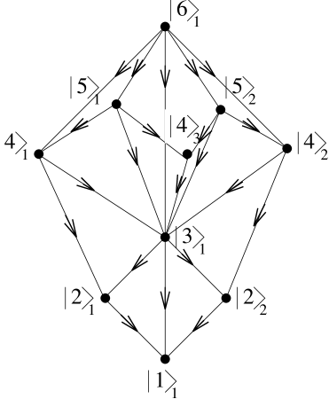
Figure 2: The topological representation of the excitation spectrum

Moreover, as the states in same level are not connected, the Hamiltonian is diagonal in that subspace. The following topological representation shows the connection of mother and daughter states in the excitation spectrum. Let us define $\nu(\eta)$ as the multiplicity of a number in a given state ket taken as a mother state. The weight of an arrow $W$ is given by the following equation:

$$W=\nu(\eta_{i})\nu(\eta_{j})$$

The following table gives the respective weights of the possible transition from the mother to daughter states.

Table 2: Transitions and weights for Calogero-Sutherland model with anti-periodic boundary condition

Transitions Weights (W) $|6\rangle_{1}\rightarrow|5\rangle_{1}$ $1\cdot 1=1$ $|6\rangle_{1}\rightarrow|5\rangle_{2}$ $1\cdot 1=1$ $|6\rangle_{1}\rightarrow|4\rangle_{1}$ $1\cdot 1=1$ $|6\rangle_{1}\rightarrow|4\rangle_{2}$ $1\cdot 1=1$ $|6\rangle_{1}\rightarrow|3\rangle_{1}$ $1\cdot 1=1$ $|5\rangle_{1}\rightarrow|4\rangle_{1}$ $2\cdot 1=2$ $|5\rangle_{1}\rightarrow|4\rangle_{3}$ $1\cdot 1=1$ $|5\rangle_{1}\rightarrow|3\rangle_{1}$ $2\cdot 1=2$ $|5\rangle_{2}\rightarrow|4\rangle_{2}$ $1\cdot 2=2$ $|5\rangle_{2}\rightarrow|4\rangle_{3}$ $1\cdot 1=1$ $|5\rangle_{2}\rightarrow|3\rangle_{1}$ $1\cdot 2=2$

Transitions Weights (W) $|4\rangle_{1}\rightarrow|3\rangle_{1}$ $2\cdot 1=2$ $|4\rangle_{1}\rightarrow|2\rangle_{1}$ $1\cdot 1=1$ $|4\rangle_{2}\rightarrow|3\rangle_{1}$ $1\cdot 2=2$ $|4\rangle_{2}\rightarrow|2\rangle_{2}$ $1\cdot 1=1$ $|4\rangle_{3}\rightarrow|3\rangle_{1}$ $2\cdot 2=4$ $|3\rangle_{1}\rightarrow|2\rangle_{1}$ $1\cdot 1=1$ $|3\rangle_{1}\rightarrow|2\rangle_{2}$ $1\cdot 1=1$ $|3\rangle_{1}\rightarrow|1\rangle_{1}$ $1\cdot 1=1$ $|2\rangle_{1}\rightarrow|1\rangle_{1}$ $3\cdot 1=3$ $|2\rangle_{2}\rightarrow|1\rangle_{1}$ $1\cdot 3=3$

III.2 Sub-family of states

Let us introduce the so-called subfamily of states which consist of the highest level mother state and all her reachable daughters. The total number of subfamily is called the dimension of the family. Since the action of Hamiltonian on a given state space generates states belonging to lower levels, the matrix representation of the Hamiltonian in a partially ordered state space is always triangular. So, the eigenvalues can be read from the diagonal elements of the matrix and there are simple algorithms to find the eigenvectors which we shall discuss later.

Finally, we see that the irreducible daughter state can be of two types

1. $|....m,m,m,.....\rangle$

2. $|....m,m,m,m-1,m-1...\rangle$

Type.1 state corresponds to the ground state with a global Galilean boost and Type.2 states corresponds to a single hole excitation.

IV The energy eigenvalue of the Hamiltonian

The energy of an eigenstate spanned by a family with the highest level mother state$|n_{1}...n_{N}\rangle$ is given by

$$E^{0}(n_{1},\dots,n_{N})=\sum_{j=1}^{N}n_{j}^{2}+A(\lambda)\sum_{j<k}(n_{j}-n_{k})$$ (16)

The off diagonal elements are found to be,

$${{}_{\mu^{\prime}}}\langle u^{\prime}|\tilde{H}|u\rangle_{{}_{\mu}}=\left\{\begin{array}[]{l}\sum_{P}\left(\prod_{i\in P}W_{i}\right)E^{1}(n_{1},\dots,n_{N})\hfill\hskip 28.45274pt\forall\mu>\mu^{\prime}\\ \hfill\\ 0\hfill\forall\mu<\mu^{\prime}\end{array}\right.$$ (17)

with

$$E^{1}(n_{1},\dots,n_{N})=2A(\lambda)\sum_{j<k}(n_{j}-n_{k})$$

The sum in equation Eq.(17) is over all possible paths $P$ from $|u\rangle_{\mu}$ and the product is over all weights $W_{i}$ of the intermediate arrows belonging to $P$. The general matrix elements of the Hamiltonian is given by,

$${{}_{\mu^{\prime}}}\langle u^{\prime}|\tilde{H}|u\rangle_{{}_{\mu}}=\varepsilon_{u^{\prime},\mu^{\prime}}^{u,\mu}$$ (18)

The energy eigenvalue can be represented in terms of a free particle momentum variable that includes the interaction term $A(\lambda)$ in a very intricate way. The full eigenspectrum of CSM can be given by,

$$E=\frac{\hbar^{2}}{2m}\sum_{j=1}^{N}k_{j}^{2}$$ (19)

Where $k_{j}$ is the so-called pseudo-momenta and is written as

$$k_{j}=\frac{1}{L^{\prime}}\left[2\pi I_{J}+\pi(A-1)\sum_{m=1}^{N}{\rm sgn}(k_{j}-k_{m})\right]$$ (20)

Here $L^{\prime}=2L$, $L$ being the length of the chain as mentioned above. The quantum numbers $I_{j}$ are now distinct half-odd integers and are related to $n_{j}$s by the following equation

$$I_{j}=n_{j}+\frac{N+1-2j}{2}$$

V The eigenfunction of the Hamiltonian

The polynomial form of the eigenfunctions of Eq.(12) is represented by Jack polynomialsjack which is symmetric over the variables $\omega_{j}$. It can be shown in fact, that the set of Jack polynomials provide a complete set of linearly independent eigenfunctions of the Hamiltonian of our present problemstanley . The formal structure of the eigenfunctions can be accomplished through the following procedure.

In order to label the symmetric polynomials we choose a sequence of nonnegative integers $\{k_{i}|i=1,\dots,N\}$, in non-increasing order i.e $k_{i}\geq 0$ for all $i$ and $k_{i}\geq k_{j}$ for all $i<j$.

The sequence is known as partitions. All nonzero $k_{j}$ are called parts. The total number of nonzero parts are called length which is denoted by $\ell(\mathbf{k})$. The weight of a partition is given by the formula

$$|\mathbf{k}|=\sum_{j=1}^{\ell(\mathbf{k})}k_{j}$$ (21)

With all the above elements we construct the so-called Young diagram $\Delta(\mathbf{k})$ giving a graphical representation of the partitions. The Young diagram $\Delta(\mathbf{k})$ is given by the following notation

$$\Delta(\mathbf{k})=\{(i,j):1\leq i\leq\ell(\mathbf{k}),1\leq j\leq k_{i}\}$$ (22)

The cell labeled by $(i,j)$ is situated in the $i$th row and the $j$th column of the Young diagram. The diagram of $\mathbf{k}$ is therefore consist of $\ell(\mathbf{k})$ rows of length $k_{j}$. The conjugate of a partition is obtained by changing all the rows of $\Delta(\mathbf{k})$ to columns in non-increasing order from left to right i.e conjugate of $\mathbf{k}$ is denoted by $\mathbf{k}^{\prime}=\{k_{1}^{\prime},k_{2}^{\prime},\dots\}$. As an obvious consequence a partition and it’s conjugate is related by the following relation

$$\sum_{i=1}^{\ell(\mathbf{k})}(i-1)k_{i}=\sum_{i=1}^{\ell(\mathbf{k}^{\prime})}\left({}^{k^{\prime}_{i}}C_{2}\right)$$ (23)

For a given cell $(i,j)$ of the Young diagram we define arm length ($a(s)$) and arm co-length ($a^{\prime}(s)$) given by the following formula

$$a(s)=k_{i}-j,\hskip 28.45274pta^{\prime}(s)=j-1$$ (24)

Similarly,the so-called leg length ($l(s)$) and leg co-length ($l^{\prime}(s)$) are given by the relations

$$l(s)=k^{\prime}_{j}-i,\hskip 28.45274ptl^{\prime}(s)=i-1$$ (25)

And finally the upper and lower hook lengths are given by

$$h^{\uparrow}_{\mathbf{k}}(s)=l(s)+\frac{1+a(s)}{A(\lambda)},\hskip 28.45274pth^{\mathbf{k}}_{\downarrow}(s)=l^{\prime}(s)+1+\frac{a(s)}{A(\lambda)}$$ (26)

The Young diagram of the example studied in section 3 is given in Fig.3 with it’s conjugate in Fig.4.

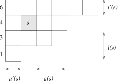
Figure 3: Young diagram for $|6,4,3,1\rangle$                           FIG. 4: Conjugate Young diagram

With the help of above definitions we obtained the orthogonality and normalization of the eigenstates of the Hamiltonian in Eq.(12). The Bosonic basis states $|\mathbf{n}\rangle$ chosen earlier in Eq.(13) are simply the monomial symmetric function and the quantum number $\mathbf{n}$ correspond to the partitions defined in the previous section. Though the quantum numbers may be negative integers, the restriction on them does not affect the construction of the eigenstates since the CSM Hamiltonian is invariant under a global Galilean transformation. Now the eigenstates can be given by so-called Jack symmetric polynomials $J^{1/A}(\omega_{i}|i=1,\dots,N)$. If ($A=1$) the Jack polynomial reduces to Schur functions describing the excitation of the free Fermionic system. At ($A=0$) it becomes the monomial symmetric function which is nothing but the free Bosonic wave function. For ($A=2,1/2$) we get the so-called zonal spherical functions. For ($A\rightarrow\infty$), $J^{1/A}$ reduces to elementary symmetric functions. Let us define a bilinear scalar product on the vector space of all symmetric function of finite degree, i.e.,

$$\langle\eta_{\mathbf{k}}\;,\;\eta_{\mathbf{n}}\rangle_{1/A}=\delta_{\mathbf{k},\mathbf{n}}\omega_{\mathbf{k}}A^{-\ell(\mathbf{k})}$$ (27)

where

$$\eta_{\mathbf{k}}=\eta_{k_{1}}\eta_{k_{2}}\eta_{k_{3}}\dots,\hskip 8.5359pt\eta_{k_{\nu}}=\sum_{j}\omega_{j}^{k_{\nu}},\hskip 8.5359pt\omega_{\mathbf{k}}=\prod_{i\geq 1}i^{m_{i}}m_{i}!,\hskip 8.5359ptm_{i}=m_{i}(\mathbf{k})$$

$\eta_{k_{\nu}}$ is a power sum symmetric function and $m_{i}(\mathbf{k})$ is the number of parts of ($\mathbf{k}=i$). Jack symmetric polynomials have the following propertiesmacd2

1. $\langle J_{\mathbf{k}},J_{\mathbf{n}}\rangle=\delta_{\mathbf{k},\mathbf{n}}j^{A}_{\mathbf{k}}$, where $j^{A}_{\mathbf{k}}$ is a normalization constant.

2. $J_{\mathbf{k}}=\sum_{\mathbf{n}}\gamma_{\mathbf{k},\mathbf{n}}\phi(\mathbf{n})$, where $\gamma_{\mathbf{k},\mathbf{n}}=0$ unless $\mathbf{k}\leq\mathbf{n}$.

3. If $|\mathbf{k}|=p$, then $\gamma_{\mathbf{k},\mathbf{n}}=p!$ where $\mathbf{k}=\{\;\underbrace{1,\dots,1}_{p}\;\}$

By the Gram-Schmidt method of orthogonalization procedure relative to the scalar product on a ring of polynomial $J_{\mathbf{k}}$ can be constructed where $j^{A}_{\mathbf{k}}$ can be given by,

$$j^{A}_{\mathbf{k}}=\prod_{s\in\mathbf{k}}h_{\mathbf{k}}^{\uparrow}(s)h_{\downarrow}^{\mathbf{k}}(s)$$

Jack polynomials are also orthogonal in the following manner,

$$\langle\mathbf{k}|\mathbf{n}\rangle_{1/A}= C_{N}^{2}\prod_{j=1}^{N}\left(\int_{0}^{L^{\prime}}dx_{j}\overline{J_{\mathbf{k}}^{1/A}}(\omega_{1},\omega_{2},\dots,\omega_{N})\right.$$

$$\left.J_{\mathbf{n}}^{1/A}(\omega_{1},\omega_{2},\dots,\omega_{N})\cdot\prod_{i<j}|\omega_{i}-\omega_{j}|^{2A}\right)$$

$$= C_{N}^{2}j^{A}_{\mathbf{k}}\prod_{s\in\mathbf{k}}\frac{N+a^{\prime}(s)/A-l^{\prime}(s)}{N+(a^{\prime}(s)+1)/A-(l^{\prime}(s)+1)}\delta_{\mathbf{k},\mathbf{n}}$$ (28)

where,

$$\omega_{j}=e^{\frac{2\pi x_{j}}{L^{\prime}}},\hskip 28.45274ptC_{N}^{2}=\left(\frac{1}{L^{\prime}}\right)^{N}\frac{\Gamma^{N}(1+A)}{\Gamma(1+AN)},\hskip 28.45274ptL^{\prime}=2L$$

and bar over $\overline{J_{\mathbf{k}}^{1/A}}$ implies complex conjugation.

VI Conclusion

In this article we obtain the energy eigenvalues and the eigenstates of the CSM with anti-periodic boundary condition. The model Hamiltonian is reduced to a convenient form by means of similarity transformations. Finally, we obtain an upper triangular representation of the Hamiltonian in terms of a partially ordered basis. The eigenstates are chosen to be symmetric polynomials known as Jack symmetric polynomials. These eigenfunctions are constructed by studying the Young diagram representation. The orthogonality and normalization of the eigenfunctions are also discussed.

References

• (1) F. Calogero, J. Math. Phys. 3 (1962) 2191, 10 (1969) 2197.
• (2) B. Sutherland, J. Math. Phys. 12 (1971) 246, 12 (1971) 251.
• (3) B. Sutherland, Phys. Rev. A 4 (1971) 2019, 5 (1972) 1372.
• (4) Z. N. C. Ha, ’Quantum Many-Body Systems in One Dimension’, World Sc., Singapore (1996).
• (5) M. Kojima, N. Ohta, Nuc. Phys. B 473 (1996) 455.
• (6) N. Ohta, J. Phys. Soc. Japan 65 (1996) 3769.
• (7) F. D. M. Halden, J. Phys C 14 (1981) 2585.
• (8) A. P. Polychronakos, Phys. Rev. Lett. 69 (1992) 703.
• (9) F. D. M. Halden, Phys. Rev. Lett. 47 (1982) 1840.
• (10) X. G. Wen, Phys. Rev. Lett. 64 (1990) 216, Phys. Rev. B 41 (1990) 12838.
• (11) X. G. Wen, Mod. Phys. Lett. B 5 (1991) 39.
• (12) A. P. Polychronakos, Nucl. Phys. B 324 (1989) 597.
• (13) F. D. M. Halden, Phys. Rev. Lett. 67 (1991) 937.
• (14) Z. N. C. Ha, Phys. Rev. Lett. 73 (1994) 1574.
• (15) P. J. Forrester, Nuc. Phys. B 388 (1992) 671.
• (16) P. J. Forrester, Phys. Lett A 179 (1993) 127.
• (17) F. J. Dyson, J. Math. Phys. 3 (1962) 140, 157, 166.
• (18) H. Jack, Proc. Roy. Soc. (Edinburgh) A 69 (1969) 1.
• (19) R. P. Stanley, Adv. Math. 77 (1989) 76.
• (20) I. G. Macdonald, Symmetric functions and Hall Polynomials, Clarendon Press (Oxford) 2nd Ed. (1995).