Rayleigh Scattering at Atoms with Dynamical Nuclei
Abstract
Scattering of photons at an atom with a dynamical nucleus is studied on the subspace of states of the system with a total energy below the threshold for ionization of the atom (Rayleigh scattering). The kinematics of the electron and the nucleus is chosen to be non-relativistic, and their spins are neglected. In a simplified model of a hydrogen atom or a one-electron ion interacting with the quantized radiation field in which the helicity of photons is neglected and the interactions between photons and the electron and nucleus are turned off at very high photon energies and at photon energies below an arbitrarily small, but fixed energy (infrared cutoff), asymptotic completeness of Rayleigh scattering is established rigorously. On the way towards proving this result, it is shown that, after coupling the electron and the nucleus to the photons, the atom still has a stable ground state, provided its center of mass velocity is smaller than the velocity of light; but its excited states are turned into resonances. The proof of asymptotic completeness then follows from extensions of a positive commutator method and of propagation estimates for the atom and the photons developed in previous papers.
The methods developed in this paper can be extended to more realistic models. It is, however, not known, at present, how to remove the infrared cutoff.
1 Introduction
During the past decade, there have been important advances in our understanding of the mathematical foundations of quantum electrodynamics with non-relativistic, quantum-mechanical matter (“non-relativistic QED”). Subtle spectral properties of the Hamiltonians generating the time evolution of atoms and molecules interacting with the quantized radiation field have been established. In particular, existence of atomic ground states and absence of stable excited states have been proven, and the energies and life times of resonances have been calculated in a rigorously controlled way, for a variety of models; see [BFS98, BFSS99, HS95, Sk98, GLL01, LL03, Gr04, AGG05, BFP05], and references given there. Furthermore, some important steps towards developing the scattering theory for systems of non-relativistic matter interacting with massless bosons, in particular photons, have been taken. Asymptotic electromagnetic field operators have been constructed in [FGS00], and wave operators for Compton scattering have been shown to exist in [Pi03]. Rayleigh scattering, i.e., the scattering of photons at atoms below their ionization threshold, has been analyzed in [FGS02] for models with an infrared cutoff. The results in this paper are based on methods developed in [DG99]. Some earlier results on Rayleigh scattering have been derived in [Sp97]. Compton scattering in models with an infrared cutoff has been studied in [FGS04]. While it is understood how to calculate scattering amplitudes for various low-energy scattering processes in models without an infrared cutoff, all known general methods to prove unitarity of the scattering matrix on subspaces of states of sufficiently low energy, i.e., asymptotic completeness, require the presence of an (arbitrarily small, but positive) infrared cutoff. In [Sp97, DG99, FGS02], Rayleigh scattering has only been studied for models of atoms with static (i.e., infinitely heavy) nuclei.
As suggested by this discussion, the main challenge in the scattering theory for non-relativistic QED presently consists in solving the following problems:
-
i)
To remove the infrared cutoff in the analysis of Rayleigh scattering;
-
ii)
to remove the infrared cutoff in the treatment of Compton scattering of photons at one freely moving electron or ion;
-
iii)
to prove asymptotic completeness of Rayleigh scattering of photons at atoms or molecules with dynamical nuclei.
In this paper, we solve problem iii) in the presence of an (arbitrarily small, but positive) infrared cutoff. In order to render our analysis, which is quite technical, as simple and transparent as possible, we consider the simplest model exhibiting all typical features and challenges encountered in an analysis of problem iii). We consider a hydrogen atom or a one-electron ion. The nucleus is described, like the electron, as a non-relativistic quantum-mechanical point particle of finite mass. We ignore the spin degrees of freedom of the electron and the nucleus. The electron and the nucleus interact with each other through an attractive two-body potential , which can be chosen to be the electrostatic Coulomb potential. Electron and nucleus are coupled to a quantized radiation field. As in [FGS02], the field quanta of the radiation field are massless bosons, which we will call photons. Physically, the radiation field is the quantized electromagnetic field. However, the helicity of the photons does not play an interesting role in our analysis, and we therefore consider scalar bosons.
As announced, we focus our attention on Rayleigh scattering; i.e., we only consider the asymptotic dynamics of states of the atom and the radiation field with energies below the threshold for break-up of the atom into a freely moving nucleus and electron, i.e., below the ionization threshold. Moreover, we introduce an infrared cutoff: Photons with an energy below a certain arbitrarily small, but positive threshold energy do not interact with the nucleus and the electron. While all our other simplifications are purely cosmetic, the presence of an infrared cutoff is crucial in our proof of asymptotic completeness (but not for most other results presented in this paper).
In the model we study, the atom can be located anywhere in physical space and can move around freely, and the Hamiltonian of the system is translation-invariant. This feature suggests to combine and extend the techniques in two previous papers, [FGS02] (Rayleigh scattering with static nuclei) and [FGS04] (Compton scattering of photons at freely moving electrons), and this is, in fact, the strategy followed in the present paper. As in [FGS04], to prove asymptotic completeness we must impose an upper bound on the energy of the state of the system that guarantees that the center of mass velocity of the atom does not exceed one third of the velocity of light. This is a purely technical restriction which we believe can be replaced by one that guarantees that the velocity of the atom is less than the velocity of light. We note that, for realistic atoms, the condition that the total energy of a state be below the ionization threshold of an atom at rest automatically guarantees that the speed of the atom in an arbitrary internal state is much less than a third of the speed of light.
Next, we describe the model studied in this paper more explicitly. The Hilbert space of pure states is given by
| (1) |
where the variables and are the positions of the nucleus and of the electron, respectively, and is the symmetric Fock space over the one-photon Hilbert space , where the variable denotes the momentum of a photon. Vectors in describe pure states of the radiation field.
The Hamiltonian generating the time evolution of states of the system is given by
| (2) |
where
| (3) |
is the Hamiltonian of the atom decoupled from the radiation field. Here and are the momentum operators of the electron and the nucleus, respectively, and and are their masses. The term is the potential of an attractive two-body force, e.g., the electrostatic Coulomb force, between the electron and the nucleus; ( is negative and tends to zero, as , and it is assumed to be such that the spectrum of is bounded from below and has at least one negative eigenvalue). The operator on the r.h.s. of (2) is the Hamiltonian of the free radiation field. It is given by
where is the energy of a photon with momentum , and , are the usual boson creation- and annihilation operators: For every function ,
are densely defined, closed operators on the Fock space , and, for , they satisfy the canonical commutation relations
where denotes the scalar product of and . For , a field operator is defined by
It is a densely defined, self-adjoint operator on . The functions (form factors) and on the right side of (2) are given by
| (4) |
where and belong to the Schwartz space, and
for some (infrared cutoff). In many of our results, we could pass to the limit ; but in our proof of asymptotic completeness of Rayleigh scattering, the condition that is essential. Finally, the parameter on r.h.s. of (2) is a coupling constant; it is assumed to be non-negative and will be chosen sufficiently small in the proofs of our results. (It should be noted that we are using units such that Planck’s constant and the speed of light , and we work with dimensionless variables chosen such that and are independent of .)
In the description of the atom, it is natural to use the following variables:
Here is the position of the center of mass of the atom, and is the position of the electron relative to the one of the nucleus. Then
| (5) |
where , , , and ; (center-of-mass momentum, relative momentum, total mass, reduced mass, respectively). Self-adjointness of on (under appropriate assumptions on ) is a standard result.
In this paper, we study the dynamics generated by on the subspace of states in whose maximal energy is below the ionization threshold
| (6) |
where is the subspace of vectors in with the property that the distance between the electron and the nucleus is at least . Vectors in with a maximal total energy below exhibit exponential decay in , the distance between the electron and the nucleus; see [Gr04]. Under our assumptions, , for a finite constant depending only on and . When then , which is the ionization threshold of a one-electron atom or -ion decoupled from the radiation field.
Our choice of the Hamiltonian , see (2) and (5), and of the form factors and , see (4), makes it clear that the dynamics of the system is space-translation invariant: Let
| (7) |
denote the momentum operator of the radiation field, and let be the total momentum operator. It is easy to check that
| (8) |
It is then useful to consider direct-integral decompositions of the space and the operator over the spectrum of the total momentum operator (which, as a set, is ). Thus
| (9) |
and
| (10) |
where the fiber Hamiltonian is the operator on the fiber Hilbert space given by
| (11) |
where is the center-of-mass momentum of the atom, and is the Hamiltonian describing the relative motion of the electron around the nucleus.
We are now in the position to summarize the main results proven in this paper for the model introduced above. In a first part, we analyze the energy spectra of the fiber Hamiltonians below a certain threshold , where is given in (6), and ; is the ground state energy of , and is a constant (speed of light, in our units). The condition guarantees that the electron is bound to the nucleus, with exponential decay in , and implies that, for a sufficiently small coupling constant , the center-of-mass velocity of the atom is smaller than the speed of light. (For center-of-mass velocities , the ground state energy of the atom decoupled from the radiation field is embedded in continuous spectrum, and the ground state becomes unstable when the coupling to the radiation field is turned on.) For realistic atoms, in particular for hydrogen, , so that is the only relevant condition. We let denote the ground state energy of , and we define
| (12) |
We prove that, for every , is a simple eigenvalue of , i.e., that the atom has a unique ground state, provided is small enough. This is a result that is expected to survive the limit , provided the factors and are not too singular at . For the Pauli-Fierz model of non-relativistic QED, existence of a ground state can be proven under conditions similar to the ones described above, provided the total charge of electrons and nucleus vanishes; see [AGG05].
By appropriately modifying Mourre theory in a form developed in [BFSS99], we prove that the spectrum of in the interval is purely continuous. With relatively little further effort, our methods would also show that is absolutely continuous. (These results, too, would survive the removal of the infrared cutoff, . This will not be shown in this paper; but see [FGSi05].)
We denote the ground state of , by ; ( is called the dressed atom (ground) state of momentum ). The space of wave packets of dressed atom states, , is the subspace of the total Hilbert space given by
| (13) |
This space is invariant under the time evolution. In fact, , where, for , , for all times .
In a second part of our paper, scattering theory is developed for the models introduced above. We first construct asymptotic photon creation- and annihilation operators
| (14) |
where is the free time evolution of a one-photon state . To ensure the existence of the strong limit on the r.h.s. of (14), we assume that , that belongs to the range of the spectral projection, , of corresponding to the interval , with , as above, and , and that the coupling constant is so small (depending on ) that the velocity of the center of mass of the atom is smaller than one. The last condition ensures that the distance between the atom and a configuration of outgoing photons increases to infinity and hence the interaction between these photons and the atom tends to , as time tends to . The details of the proof of (14) are very similar to those in [FGS00]. From (13) and (14) we infer that, for , and under the conditions of existence of the limit in (14), vectors of the form exist, and their time evolution is the one of freely moving photons and a freely moving atom:
| (15) |
as . Furthermore, , under the same assumptions. Equation (15) provides the justification for calling the vectors scattering states. We already know that the atom does not have any stable excited states. It is therefore natural to expect that the time evolution of an arbitrary vector in the range of the spectral projection , with as above, approaches a vector describing a configuration of freely moving photons and a freely moving atom in its ground state, as time tends to . Thus, with (15) and (13), we expect that, for ,
| (16) |
where denotes the linear subspace spanned by a set, , of vectors in , and denotes the closure of in the norm of . Property (16) is called asymptotic completeness of Rayleigh scattering. The main result of this paper is a proof of (16) under the supplementary condition that for some (the proof of (16) is the only part of the paper where, for technical reasons, we need to assume ; all other results only require ). Next, we reformulate (16) in a more convenient language. We define a Hilbert space of scattering states as the space , and we introduce an asymptotic Hamilton operator, , by setting
| (17) |
where
| (18) |
for arbitrary , with , as above. On the range of , the operators , given by
| (19) |
exist; see (14). The vector is the vacuum in the Fock-space characterized by the property that , for . The operators and are called wave operators, and the scattering matrix is defined by
| (20) |
From Eqs. (14) and (15) we find that
and hence the ranges of and are contained in the range of . Using that , for and , one sees that and are isometries from the range of into . If we succeeded in proving that
| (21) |
we would have established the unitarity of the -matrix, defined in (20), on , i.e., asymptotic completeness of Rayleigh scattering.
In order to prove (21), we show that have right inverses defined on . Our proof is inspired by proofs of similar results in [DG99] and in [FGS02, FGS04]. It is based on constructing a so called asymptotic observable and then proving that is positive on the orthogonal complement of in . The proof of this last result is, perhaps, the most original accomplishment in this paper and is based on some new ideas.
Our paper is organized as follows. In Section 2, we define our model more precisely, and we state our assumptions on the potential and on the form factors and . In Section 3, we study the spectrum of the fiber Hamiltonian : In Section 3.1, we prove the existence of dressed atom states, and, in Section 3.3, we prove two positive commutator estimates, from which we conclude that the spectrum of above the ground state energy and below an appropriate threshold is continuous. In Section 4, we discuss the scattering theory of the system. First, in Section 4.1, we prove the existence of asymptotic field operators, we recall some of their properties, we prove the existence of the wave operators, and we state our main theorem. Then, in Section 4.2, we introduce a modified Hamiltonian, , describing “massive” photons, and we explain why it is enough to prove asymptotic completeness for instead of . In Section 4.3, we construct asymptotic observables and inverse wave operators . In Section 4.4, we prove positivity of our asymptotic observables when restricted to the orthogonal complement of (the space of wave packets of dressed atom states). Finally, in Section 4.5, we complete the proof of asymptotic completeness. In Appendix A, we introduce some notation, used throughout the paper, concerning operators on the bosonic Fock space. In Appendix B, we summarize bounds used to control the interaction between the electron (or the nucleus) and the radiation field.
2 The Model
We consider a non-relativistic atom consisting of a nucleus and an electron interacting through a two-body potential . The Hamiltonian describing the dynamics of the atom is the self-adjoint operator
| (22) |
acting on the Hilbert space , where and denote the position of the nucleus and of the electron, respectively, and and are the corresponding momenta. We assume that the interaction potential satisfies the following assumptions.
Hypothesis (H0): The potential is a locally square integrable function, with , and such that is infinitesimally small with respect to the Laplace operator , in the sense that, for all there exists a finite constant such that
(23) for every . Moreover the potential is such that the ground state energy of the Schrödinger operator (with ) is non-degenerate.
Remarks.
-
1)
Hypothesis (H0) is satisfied by the Coulomb potential and it is inspired by this potential. It follows from (H0) that the Hamiltonian with domain is a self-adjoint operator on the Hilbert space and that it is bounded from below.
-
2)
With little more effort we could have covered a much larger class of locally square integrable potentials where only the negative part is infinitesimally small with respect to and is self-adjointly realized in terms of a Friedrich’s extension. This would allow, e.g., for confining potentials that tend to as .
-
3)
Note that we are neglecting the degrees of freedom corresponding to the spin of the nucleus and of the electron, because they do not play an interesting role in the scattering process.
Next we couple the atom to a quantized scalar radiation field. We call the particles described by the quantized field (scalar) photons. The pure states of the photon field are vectors in the bosonic Fock space over the one-particle space ,
| (24) |
where denotes the subspace of consisting of all functions which are completely symmetric under permutations of the arguments. The variables denote the momenta of the photons.
The dispersion relation of the photons is given by , which characterizes relativistic particles with zero mass. The free Hamiltonian of the quantized radiation field is given by the second quantization of , denoted by . Formally,
| (25) |
where and are the usual creation- and annihilation operators on , satisfying the canonical commutation relations , . More notations for operators on Fock space that are used throughout the paper are collected in Appendix A.
The total system, atom plus quantized radiation field, has the Hilbert space ; its dynamics is generated by the Hamiltonian
| (26) |
where is a real non-negative coupling constant (the assumption is not needed, it just makes the notation a little bit simpler), and where
| (27) |
The form factors and are square integrable functions of with values in the multiplication operators on . Clearly, describes the interaction between the electron and the radiation field, and couples the field to the nucleus. The next hypothesis specifies our assumptions on the form factors and .
Hypothesis (H1): The form factors and have the form
(28) where belong to Schwartz space , and if , for some .
The particular form of and given in (28) guarantees the translation invariance of the system (see the discussion after (38)). The presence of an infrared cutoff in and is used in the proofs of many of our results; but it is not necessary for the existence of the asymptotic field operators and for the existence of the wave operator in Section 4.1. Notice that, even though our main results require the coupling constant to be sufficiently small, how small has to be does not depend on the infrared cutoff , in the following sense. If we define and , with , and with monotone increasing and such that if and if , then Hypothesis (H1) is satisfied for every choice of . Moreover how small has to be is independent of the choice of the parameter .
Assuming Hypotheses (H0) and (H1), the Hamiltonian , defined on the domain , is essentially self-adjoint and bounded from below. This follows from Lemma 20, which shows, using Hypothesis (H1), that the interaction is infinitesimal with respect to the free Hamiltonian .
To study the system described by the Hamiltonian , it is more convenient to use coordinates describing the center of mass of the atom and the relative position of the nucleus and the electron. We define
| (29) |
Then, the atomic Hamiltonian becomes
| (30) |
where is the center of mass momentum of the atom, and is the momentum conjugate to the relative coordinate . Moreover, is the total atomic mass, and is the reduced mass. Expressed in the new coordinates, the total Hamiltonian of the system is given by
| (31) |
Here and , and we use the notation
| (32) |
with
| (33) |
The fact that the form factors and contain an infrared cutoff (meaning that , if ) implies that photons with very small momenta do not interact with the atom. In other words, they decouple from the rest of the system. We denote by (the subscript stands for “interacting”) the characteristic function of the set . Then the operator , whose action on the -particle sector of is given by
| (34) |
defines the orthogonal projection onto states without soft bosons. The fact that soft bosons do not interact with the atom implies that leaves the range of invariant; commutes with . Another way to isolate the soft, non-interacting, photons from the rest of the system is as follows. We have that , where is the open ball of radius around the origin and denotes its complement. Hence the Fock space can be decomposed as , where is the bosonic Fock space over (describing interacting photons), and is the bosonic Fock space over (describing soft, non-interacting, photons). Accordingly, the Hilbert space can be decomposed as
| (35) |
By we denote the unitary map from to . The action of the Hamiltonian on is then given by
| (36) |
with
| (37) |
Note that in the representation of the system on the Hilbert space , the projection (projecting on states without soft bosons) is simply given by , where denotes the orthogonal projection onto the vacuum in .
One of the most important properties of the Hamiltonian is its invariance with respect to translations of the whole system, atom and field. More precisely, defining the total momentum of the system by
| (38) |
we have that . Because of this property, it can be useful to rewrite the Hilbert space as a direct integral over fibers with fixed total momentum. Specifically, we define the isomorphism
| (39) |
as follows. For , we define
| (40) |
with
| (41) |
where
| (42) |
is the Fourier transform of with respect to its first variable. Because of its translation invariance, the Hamiltonian leaves invariant each fiber with fixed total momentum of the Hilbert space . More precisely,
| (43) |
where we put . Recall that .
Note that, for every fixed , the operator is a self-adjoint operator on the fiber space . Our first results, stated in the next section, describe the structure of the spectrum of the fiber-Hamiltonian , for fixed values of .
3 The Spectrum of
3.1 Dressed Atom States
The first question arising in the analysis of the spectrum of
| (44) |
concerns the existence of a ground state of : we wish to know whether or not is an eigenvalue of . We will answer this question affirmatively, under the assumption that the energy lies below some threshold and that the coupling constant is sufficiently small. The restriction to small energies is necessary to guarantee that the center of mass of the atom does not move faster than with the speed of light ( in our units), and that the atom is not ionized. The following lemma (and its corollary) proves that an upper bound on the total energy is sufficient to bound the momentum of the center of mass of the atom (provided the coupling constant is sufficiently small) and to make sure that the electron is exponentially localized near the nucleus.
Lemma 1.
Assume that Hypotheses (H0) and (H1) are satisfied.
-
i)
Define , and fix . Suppose . Then there is such that
(45) for all , and for all . In particular .
-
ii)
Define the ionization threshold
with . Let be such that . Then
(46)
Proof.
i) Fix such that . Choose such that for , and if . Then we have that
| (47) |
where is the non-interacting fiber Hamiltonian and where the constant is independent of . To prove the last equation note that, if denotes an almost analytic extension of (see Appendix A in [FGS04] for a short introduction to the Helffer-Sjöstrand functional calculus), we have that
| (48) |
and therefore
| (49) |
uniformly in . Next, since , , and by the definition of , we have that
Since , we conclude from (47) that
for sufficiently small (independently of ).
As for part ii), we use Theorem 1 of [Gr04] and an estimate from its proof. Given and , let
where and . Suppose for a moment that
| (50) |
for all and all . Then and hence
by [Gr04, Theorem 1]. Moreover, the value of the parameter in the proof of [Gr04, Theorem 1], in the case of the Hamiltonian , can be chosen independent of thanks to (50). It follows that the estimate for from that proof is also independent of . It thus remains to prove (50). To this end we proceed by contradiction, assuming that (50) is wrong. Then there exist and such that
Hence, we find with and with
| (51) |
Moreover, since the map , for fixed , is continuous in (it is just a quadratic function in ), there exists such that
for all with . Next, we choose (where denotes the ball of radius around ) with , and we define by
From (51), we obtain that
| (52) |
because . Since (which is clear from the construction of ), this contradicts the definition of . ∎
In the next proposition we prove the existence of a simple ground state for , provided the energy is lower than a threshold energy and the coupling constant is small enough.
Proposition 2.
Assume Hypotheses (H0) and (H1) are satisfied. Fix and choose (see Lemma 1 for the definition of and ). Then, for sufficiently small (depending on and ), is a simple eigenvalue of , provided that .
Remark. Since it suffices that and that is small enough.
Proof.
The proof is very similar to the proof of Theorem 4 in [FGS04]. For completeness we repeat the main ideas, but we omit details. In order to prove the proposition, we consider the modified Hamiltonian (defined in Section 4.2) given, on the fiber with fixed total momentum , by
| (53) |
where the dispersion law (with if and for all ) is assumed to satisfy Hypothesis (H2) of Section 4.2. Set . Note that and act identically on the range of , the orthogonal projection onto the subspace of vectors without soft bosons.
The proof of the proposition is divided into four steps.
-
1)
Suppose . Then, for sufficiently small (depending on and ), we have that
(54) for every . This inequality follows by perturbation of the free Hamiltonian (see Lemma 35 in [FGS04] for details).
-
2)
. Moreover, if is an eigenvector of (or of ) corresponding to the eigenvalue , then . In particular, is an eigenvector of corresponding to the eigenvalue if and only if is an eigenvector of corresponding to the eigenvalue .
In order to prove these statements note that the Hamiltonians and act on the fiber space , where is the Fock space of the soft bosons, . Thus
The restriction of to the subspace with exactly soft bosons is given by
with
| (55) |
In the last inequality we used the result of part (1). This proves that
| (56) |
Since , we conclude that . Eq. (55) also proves that eigenvectors of corresponding to the energy , if they exist, belong to the range of . That the same is true for eigenvectors of corresponding to the energy follows from an inequality for analogous to (55).
-
3)
If , and for sufficiently small (depending on and ) we have that
(57)
For , this follows from part (1) (because ), while for , this inequality follows from , by (54) and by construction of (see Section 4.2).
-
4)
(58) where is defined like with replaced by . (Recall from 2) that ).
The proof of part 4) is very similar to the proof of Lemma 36 in [FGS04] with a small modification at the beginning. We first need to localize with respect to the relative coordinate . That is, we choose with for , for and . Let . Then
| (59) |
as . As in [FGS04], one shows that
with relatively compact w.r.t. , while
as follows from the definition of . Part 4) follows from these estimates applied to the r.h.s. of (59).
From now on, for fixed and such that , we denote by the unique (up to a phase) normalized ground state vector of . The vector is called a dressed atom state with fixed total momentum . The space of dressed atom wave packets, , is defined by
where is the one-dimensional space spanned by the vector ; is a closed linear subspace left invariant by the Hamiltonian . In fact, commutes with the orthogonal projection , onto . This follows from .
3.2 The Fermi Golden Rule
From Hypothesis (H0), and from standard results in the theory of Schrödinger operators (see [RS78]), it follows that the spectrum of
in the negative half-axis is discrete. We denote the negative eigenvalues of by . The eigenvalues can accumulate at zero only. If has no eigenvalues (a possibility which is not excluded by our assumptions), then our results (which only concern states of the system for which the electron is bound to the nucleus) are trivial. We denote the (finite) multiplicity of the eigenvalue by . For fixed , we denote by , , an orthonormal basis of the eigenspace of corresponding to the eigenvalue . By Hypothesis (H0), the lowest eigenvalue, , of is simple (). The unique (up to a phase) ground state vector of is denoted by .
For every fixed , the free Hamiltonian,
| (60) |
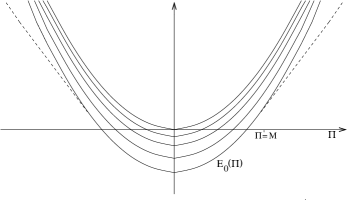
has eigenvalues
with multiplicity corresponding to the eigenvectors (where denotes the Fock vacuum), for every . For , , while all other eigenvalues , , are embedded in the continuous spectrum (see Fig. 1).
For , all eigenvalues of are embedded in the continuous spectrum, and the Hamiltonian does not have a ground state. We restrict our attention to the physically more interesting case ; (this will be ensured by the condition that the total energy of the system is less than and that the coupling constant is sufficiently small). One then expects the embedded eigenvalues , , to dissolve and to turn into resonances when the perturbation is switched on. We prove that this is indeed the case, provided the lifetime of the resonances, as predicted by Fermi’s Golden Rule in second order perturbation theory, is finite.
For given and , we define the matrix
| (61) |
For given , we then define the resonance matrix by setting
| (62) |
where denotes the Dirac delta-function. Note that is an matrix. According to second order perturbation theory (Fermi’s Golden Rule), the eigenvalues of are inverses of the lifetimes of the resonances bifurcating from the unperturbed eigenvalue . We put
| (63) |
Instability of the eigenvalue is equivalent, in second order perturbation theory, to the statement that .
Hypothesis (H2): For fixed and , we assume that
(64)
3.3 The Positive Commutator
In order to prove the absence of embedded eigenvalues we use the technique of positive commutators. We prove the positivity of the commutator between the Hamiltonian and a suitable conjugate operator . Then the absence of eigenvalues follows with the help of a virial theorem. We make use of ideas from [BFSS99], adapting them to our problem.
For fixed , we construct a suitable conjugate operator , and, in Proposition 3, we prove the positivity of the commutator when restricted to an energy interval containing the unperturbed eigenvalue but no other eigenvalues of . In Proposition 4, we then establish a commutator estimate on an energy interval around the ground state energy of .
For fixed we define
| (65) |
By definition, is the orthogonal projection onto the eigenspace of corresponding to the eigenvalue . We also define the symmetric operator
| (66) |
where
| (67) |
and
| (68) |
In (68), we introduced the notation and we used
| (69) |
Note that strongly, as . The real parameters and will be fixed later on.
Proposition 3.
We assume that Hypotheses (H0)-(H2) are satisfied. We fix and choose ; (see Lemma 1 for the definition of and ). Moreover, we suppose that the interval is such that and
| (70) |
Then, for sufficiently small (depending on , and the distance ), one can choose and such that
| (71) |
with a positive constant .
Remarks.
-
1)
The choice of the parameter and of the constant depends on the value of . We can choose, for example,
for .
- 2)
-
3)
In this proposition, we do not need the infrared cutoff in the interaction (i.e., we can choose ). However, the infrared cutoff is needed in the proof of Proposition 5 (the Virial Theorem), and hence in the proof of the absence of embedded eigenvalues.
Proof.
We begin with a formal computation of the commutator :
Recall that . Using Eq. (45), it is easy to check that, for as above,
| (72) |
Thus, defining
| (73) |
we conclude that
| (74) |
and it is enough to prove the positivity of the r.h.s. of the last equation to complete the proof. The advantage of working with , instead of the commutator , is that is bounded with respect to the Hamiltonian while is not (since the number operator is not bounded with respect to ). In order to prove that
| (75) |
we first establish the inequality
| (76) |
To this end we may assume that
| (77) |
for otherwise (76) holds with . This assumption will allow us to apply the Feshbach map with projection to the operator . Indeed, this operator restricted to is invertible for small and as is shown in Step 1. Step 1 through Step 5 prepare the proof of (76).
Step 1. There exists a constant , independent of and , such that
| (78) |
In fact,
| (79) |
Applying Lemma 21 of Appendix B to bound , using that (by the choice of the interval ), and that , inequality (78) follows easily.
Step 2. We define
| (80) |
where is defined in (77) (note that, by (77) and by the result of Step 1, the inverse on the r.h.s. of (80) is well defined, if and are small enough). Then we have
| (81) |
The proof of (81) relies on the isospectrality of the Feshbach map and can be found, for example, in [BFSS99]. This inequality says that, instead of finding a bound on the operator restricted to the range of , we can study the operator restricted to the much smaller range of the projection (which is finite-dimensional).
Using the assumption (77) and Eq. (78), we see that, if and are sufficiently small,
| (82) |
(Later, when we will choose the parameter and , we will make sure that is small enough, if is small enough). This implies that the operator is bounded from below by
| (83) |
Next, we study the second term on the r.h.s. of inequality (83).
Step 3. There exists a constant independent of and such that
| (84) |
In order to prove this bound, we note that, for any ,
| (85) |
Furthermore
| (86) |
because
Hence we find that
| (87) |
Using Lemma 21 and the bound , we conclude that
| (88) |
Taking the square of this inequality, we obtain (84).
Step 4. We show that
| (89) |
Using that and , we easily find that
| (90) |
Writing , using that commutes with , and that we find
| (91) |
Eq. (89) now follows writing and using that .
Step 5. Next, we claim that
| (93) |
where , as .
In order to prove (93), we use the pull-through formula for and the fact that . This yields
| (94) |
Next, we write , where is the orthogonal projection onto the eigenspace of corresponding to the eigenvalue . Then we obtain that
| (95) |
All operators involved in the expression on the r.h.s. of (95) act trivially on the Fock space, and we get the lower bound
| (96) |
Using that , as , and recalling the definition of the matrix , we find that
| (97) |
This proves Eq. (93).
Proof of Eq. (76). From (92) and (93), we derive that
| (98) |
Choosing and , with , we get
| (99) |
for sufficiently small. Note that, with this choice of and , , and thus (82) is satisfied, if is small enough. From (77) and (81) we then get that
| (100) |
which proves (76).
Proof of Eq. (75). To prove (75), and hence complete the proof of the proposition, we must replace by the spectral projection of the full Hamiltonian .
Given an interval with and
| (101) |
we choose an interval such that , and
| (102) |
and with . Furthermore, we choose a function with the property that on and on . We can assume that . Applying (100) with replaced by , and multiplying the resulting inequality with we get
| (103) |
Setting and , we have that
| (104) |
Using
| (105) |
we find that
| (106) |
Next we use that
| (107) |
From the definition of it follows that
with the choice , . This implies that
| (108) |
where the constant depends on ( is proportional to ). Thus, with (106),
| (109) |
Since , we have and . Therefore, multiplying from the left and the right with , and choosing small enough, we find that
| (110) |
for some positive constant , which, with (74), completes the proof of the proposition. ∎
Proposition 3 and Proposition 5, below, prove absence of embedded eigenvalues of on with the exception of a small interval around the ground state energy, . Absence of embedded eigenvalues near the ground state energy follows from our next proposition.
Proposition 4.
Assume Hypotheses (H0)-(H1). Fix , and choose , with . Suppose the interval is such that
| (111) |
(Recall that denotes the first excited eigenvalue of the free Hamiltonian ). Then, if is sufficiently small (depending on , and ), there exists such that
| (112) |
Proof.
A simple calculation shows that
| (113) |
Hence
| (114) |
Here we use that, by Hypothesis (H1), , and that, by Lemma 21, .
Next, we note that
| (115) |
where is the unique (up to a phase) ground state vector of the atomic Hamiltonian . Next we choose a function with for and for . Eq. (115) then implies that
| (116) |
Note that
| (117) |
Since, by definition of the interval , , we find that
| (118) |
With (114) and (116), this shows that
| (119) |
∎
Proposition 5 (Virial Theorem).
Proof.
To prove the proposition, we replace the Hamiltonian by a modified Hamiltonian
where the new dispersion law satisfies , for , and for all . Since the two Hamiltonian and act identically on states without soft bosons (in the range of the projection ), it is enough to prove that
| (120) |
and
| (121) |
where , and equals with replaced by . The proof of (120) is very similar to the proof of Lemma 40, in [FGS04]. The proof of (121) follows easily from (120), because is a bounded operator on . ∎
Corollary 6.
Assume Hypotheses (H0)-(H2). Fix and choose , with and as in Lemma 1. Then, for sufficiently small values of ,
| (122) |
where is a simple eigenvalue, for all with .
Remark. How small has to be chosen depends on the choice of (), on the choice of (we need (45) to hold true), on (), and it also depends on the distances between the eigenvalues of the atomic Hamiltonian (we must require that , where is such that ).
Proof.
We first prove that if is sufficiently small, then
| (123) |
and that is a simple eigenvalue of .
To this end, we define . We define intervals
for , where is such that . Each interval contains exactly one eigenvalue of the free Hamiltonian , and . The absence of eigenvalues of inside , for and for sufficiently small, follows from Propositions 3 and 5. Next, suppose that is a normalized eigenvector of corresponding to an eigenvalue . Without loss of generality, we can assume that is real; recall that is the unique (up to a phase) normalized ground state vector of . Then, by Proposition 4 and Proposition 5, we have that
| (124) |
Hence
| (125) |
If there were two orthogonal eigenvectors of , and , corresponding to eigenvalues in then both would satisfy inequality (125), and, thus, we would conclude that
| (126) |
But this is impossible if . So, for small enough, there can only be one eigenvector of corresponding to an eigenvalue in . In Proposition 2, we have proven that has a ground state vector. This proves the fact that is a simple eigenvalue of as well as the fact that has no other eigenvalue in . Hence (123) follows. To complete the proof of the corollary, we need to show that
| (127) |
To this end, we decompose , and we write , where
is the space of vectors containing exactly soft, non-interacting, bosons. The Hamiltonian leaves each invariant, and the restriction of on is given by
| (128) |
Here is an operator over , the space of states with no soft bosons. We know that the only eigenvalue of in is its ground state energy as long as . In particular the only eigenvalue of in is given by if this number is less than . Thus is an eigenvalue of if and only if there exists a set with positive measure, such that
| (129) |
for all . But this is impossible because
for every with and small enough. ∎
4 Scattering Theory
The proofs of most of the results in this section are similar to those of the corresponding results in [FGS04]. In order to give an idea of the structure of the proof of our main result (asymptotic completeness, Theorem 9), we repeat here the most important theorems, but we omit most of their proofs (we refer to the corresponding statements in [FGS04]). The main difference with respect to [FGS04] is encountered in the proof of the positivity of the asymptotic observable in Section 4.4: there, we propose some new ideas to control the internal degrees of freedom of the atom (which are not present in [FGS04], because there we considered free electrons coupled to the quantized radiation field).
4.1 The Wave Operator
The first step towards understanding scattering theory for the model studied in this paper consists in the construction of states with asymptotically free photons. This can be accomplished using asymptotic field operators, which are constructed in the next theorem. Note that in Theorems 7 and 8 we do not impose any infrared cutoff on the interaction; we can take , provided the form factor is smooth at . We use the notation .
Theorem 7 (Existence of asymptotic field operators).
Assume Hypotheses (H0)-(H1) are satisfied (but is allowed!). Fix and choose (with as in Lemma 1). If is so small that (45) is true, then the following results hold.
-
i)
Let and let . Then the limit
exists for all .
-
ii)
Let . Then
in the sense of quadratic forms on ( means either or ).
-
iii)
Let , and let and . Then
if .
-
iv)
Let for . Put and assume . Then if we have that , the limits
exist, and
-
v)
If and ,
(Wave packets of dressed atom states are vacua of the asymptotic field operators).
The proof of this theorem is very similar to the one of Theorem 13 and Lemma 14 in [FGS04]. It relies on a propagation estimate for the center of mass of the atom (see Proposition 12 in [FGS04]), which guarantees that if the energy is smaller than , then the asymptotic velocity of the atom is bounded above by (here ), and it exploits the fact that, because the energy is below the ionization threshold, the electron is exponentially bound to the nucleus. These two facts and the fact that the propagation speed of photons is the speed of light are sufficient to prove that the interaction between the atom and asymptotically freely propagating photons tends to zero, as .
The existence of asymptotic field operators allows us to introduce the wave operator of the system. In order to define , we add a new copy of the Fock space describing states of free photons to the physical Hilbert space . We define the extended Hamiltonian
| (130) |
on the extended Hilbert space . In the next theorem, we establish the existence of the wave operator as an isometry from a subspace of to a subspace of the physical Hilbert space . The “scattering identification map”, , used in the definition of the wave operator , is defined in Appendix A.6.
Theorem 8 (Existence of the wave operator).
Let Hypotheses (H0)-(H1) be satisfied (but is allowed). Fix , and choose (with defined as in Lemma 1). Then if is small enough (depending on and ) the limit
| (131) |
exists for an arbitrary vector in the dense subspace of spanned by finite linear combinations of vectors of the form , where , , and with . If belongs to this space then
| (132) |
Furthermore , and has therefore a unique extension, also denoted by , to . On , the operator is isometric. For all ,
For the proof of this theorem we refer to the proof of Theorem 15 in [FGS04], which is almost identical. From Eq. (132) we see that vectors in the range of are limits of linear combination of vectors describing wave packet of dressed atom states and configurations of finitely many asymptotically freely moving photons. Physically, it is expected that the asymptotic evolution of every state with an energy below the ionization threshold of the atom (that is ) and so small that the atom does not propagate with a velocity larger than one (i.e., ) can be approximated by linear combinations of vectors describing a dressed atom state and a configuration of finitely many freely propagating photons. More precisely, one expects that
This statement is called asymptotic completeness of Rayleigh scattering. Due to technical difficulties, we can only prove asymptotic completeness for states with energy less than a threshold energy and assuming that the coupling constant is small enough. The following theorem is our main result.
Theorem 9 (Asymptotic Completeness).
Remark. The allowed range of values of depends on the value of ; (we need that ), on the choice of ( must be small enough in order for Eq. (45) to hold true), on the value of (), and on , with such that (). As remarked in Section 2, the assumption that is positive is not necessary, it only simplifies the notation (but is not allowed, because in this case the fiber Hamiltonian has embedded eigenvalues).
4.2 The Modified Hamiltonian
The fact that the bosons are massless leads to some technical difficulties connected with the unboundedness of the operator with respect to the Hamiltonian. However, as long as the infrared cutoff is strictly positive, the number of bosons with energy below is conserved. This allows us to introduce a modified Hamiltonian, where the dispersion law of the soft, non-interacting, photons is changed. We define
and we assume that the dispersion law has the following properties.
Hypothesis (H3). , with , , for , , for all , , and unless . Furthermore, for all . (Here is the infrared cutoff defined in Hypothesis (H1).)
The two Hamiltonians, and , agree on states of the system without soft bosons. Recall that is the characteristic function of the set and that the operator is the orthogonal projection onto the subspace of vectors describing states without soft bosons. It is straightforward to check that and leave the range of the projection invariant and that
| (133) |
The same conclusion can be reached using the unitary operator introduced in Section 2. On the factorized Hilbert space , the Hamiltonians and are given by
| (134) |
and we see explicitly that the two Hamiltonians agree on states without soft bosons.
The modified Hamiltonian , just like the physical Hamiltonian , commutes with spatial translations, i.e., , where is the total momentum of the system. In the representation of the system on the Hilbert space , the modified Hamiltonian is given by
where has been defined in Section 2.
The fiber Hamiltonians and commute with the projection and agree on its range,
| (135) |
In the proof of Proposition 2 we have shown that if and then, for small enough,
where is a simple eigenvalue of and of , as long as . Moreover, the corresponding dressed atom states coincide. Since the subspace is defined in terms of the dressed atom states , it follows that vectors in also describe dressed atom wave packets for the dynamics generated by the modified Hamiltonian .
Next, we discuss the scattering theory for the modified Hamiltonian . As in Theorem 8 we fix and we choose . Then, by the assumption that for , and since commutes with and we have that
| (136) |
for all . It follows that the limit
exists and that , for all and for all . This and the fact that vectors in describe dressed atom states for and for show that the asymptotic states constructed with the help of the Hamiltonians and coincide.
On the extended Hilbert space , we define the extended modified Hamiltonian
In terms of and we also define a modified version, , of the wave operator introduced in Section 4.1.
Lemma 10.
Let Hypotheses (H0), (H1) and (H3) be satisfied ( in Hypothesis (H1) is allowed, and then ). Fix and . Then if is sufficiently small, depending on and , the limit
| (137) |
exists for all . Moreover, the modified wave operator , defined by , agrees with on . That is,
| (138) |
for all .
We now extend the domain of to include arbitrarily many soft, non-interacting bosons. As a byproduct we obtain a proof of (138). To start with, we recall the isomorphism introduced in Section 2 and define a unitary isomorphism separating interacting from soft bosons in the extended Hilbert space . With respect to this factorization the extended Hamiltonian becomes , where . As an operator from to , the wave operator acts as
| (139) |
where is given by
| (140) |
while is given by
| (141) |
where is the orthogonal projection onto the vacuum vector . In view of (139) and (140), the domain of can obviously be extended to . For the modified wave operator , we have , and from it follows that . Consequently, also is well defined on and .
We summarize the main conclusions in a lemma.
Lemma 11.
Let the assumptions of Lemma 10 be satisfied, and let be defined on , as explained above. Then
| (142) |
in the factorization . In particular, the following statements are equivalent:
-
i)
.
-
ii)
.
-
iii)
.
-
iv)
.
4.3 Existence of the Asymptotic Observable and of the Inverse Wave Operator
Fix and choose (recall from Lemma 1 that ). We choose numbers and such that
Definition. We pick a function such that on and on . Our asymptotic observable is defined by
where the energy cutoff is smooth and supported in . For the existence of this limit, see Proposition 13 below.
The physical meaning of the asymptotic observable is easy to understand: measures the number of photons that are propagating with an asymptotic velocity larger than . We will prove in Section 4.4 that is positive when restricted to the subspace of vectors orthogonal to the space of wave packets of dressed atom states. Instead of inverting the wave operator directly, we can then invert it with respect to the asymptotic observable . More precisely, we define an operator , called the inverse wave operator, such that . Then, using the positivity of , we can construct an inverse of . In order to define , we need to split each boson state into two parts, the second part being mapped to the second Fock-space of prospective asymptotically freely moving bosons.
Definition. We define as follows: let , where , , , on , while on and . Then the inverse wave operator is given by
where is a smooth energy cutoff supported in . See Appendix A.5 for the definition of the operator . For the existence of this limit, see Proposition 14.
Note that, since by definition , the photons which propagate with velocity larger than are asymptotically free. To prove this fact, notice first that Lemma 1 continues to hold with replaced by . Hence, the assumption that (where is the energy cutoff appearing in the definition of and ) with guarantees, for sufficiently small , that both the nucleus and the electron remain inside a ball of radius around the origin. In fact, using the assumption (and small enough), we can prove, analogously to Proposition 12 in [FGS04], that
| (143) |
for any with , and for any with . Recall that is the coordinate of the center of mass of the atom. Moreover, the assumption that implies that the electron and the nucleus remain exponentially bound for all times; therefore, both the electron and the nucleus are localized inside the ball of radius . As a consequence, the interaction strength between the nucleus (or the electron) and those bosons counted by decays in at an integrable rate. To establish this fact rigorously we need the following lemma, similar to Lemma 9 in [FGS04].
Lemma 12.
Assume that Hypothesis (H1) is satisfied and that . Then, for every , there exists a constant such that
| (144) |
Moreover, if , we have
| (145) |
Remark. In the proof of the existence of the operators and , where we use this lemma, typically and . Hence the r.h.s. of (145) gives a decay in time which is integrable if we choose large enough.
Proof.
To prove (144), we first choose , with (recall that and ) and we observe that
| (146) |
Using that , it follows that
| (147) |
Hence the second term on the r.h.s. of (146) can be bounded by (because is bounded). Moreover the square of the first term on the r.h.s. of (146) can be estimated by
| (148) |
for all and . Here we used that, from , , and since, by definition of , and , we have that and analogously . Since , their Fourier transform decay faster than any power, and hence (148) implies (144).
The decay of the interaction determined in the last lemma is one of the two key ingredients for proving the existence of and . The other one is a propagation estimate for the photons, analogous to Proposition 24 in [FGS04], but with the cutoff for (in [FGS04], is the position of the electron) replaced by a cutoff for the asymptotic velocity of the center of mass of the nucleus-electron compound (the reason why we can introduce here a cutoff in is that, because of (143), we know it can not exceed ).
For the details of the proof of the next two proposition we refer to Theorems 26 and 28 in [FGS04].
Proposition 13 (Existence of the asymptotic observable).
Assume that Hypotheses (H0), (H1) and (H3) are satisfied. Fix , and choose . Suppose that with . Let , and be as defined above, and let be the operator of multiplication with . Then, for small enough (in order for (45) to hold true),
exists, and commutes with . Here .
Proposition 14 (Existence of ).
Assume Hypotheses (H0), (H1) and (H3) are satisfied. Fix and choose . Suppose that with , and that and are defined as described above. If is so small that (45) holds, then
-
(i)
the limit
exists, and , for all ;
-
(ii)
;
-
(iii)
.
4.4 Positivity of the Asymptotic Observable and Asymptotic Completeness
In this section we prove the positivity of the asymptotic observable , restricted to the subspace of states orthogonal to wave packets of dressed atom states and not containing any soft bosons. We need the following lemma.
Lemma 15.
Assume Hypotheses (H0), (H1), (H3). Fix and choose . Suppose, moreover, that and . Put , where is the position of the center of mass of the atom. Then, if is so small that (45) holds true, we have that
| (150) |
on the range of the projection .
This lemma follows from a straightforward estimate of the commutator , from (45), (46), and from Lemma 21.
Theorem 16 (Positivity of the asymptotic observable).
Assume that Hypotheses (H0)-(H3) are satisfied. Fix and choose (with and as in Lemma 1). Let the operator be defined as in Proposition 13 with . Then if is sufficiently small we can choose in the definition of such that
| (151) |
Here is a positive constant depending on , , , but independent of . In particular, if and then on , then
| (152) |
Proof.
Let . Since is dense in , it is enough to prove that
| (153) |
for every . As before, we use the notation .
The first step consists in proving that there exists a constant , depending only on , such that, for every and for every ,
| (154) |
This inequality can be established as in the proof of Theorem 27 in [FGS04]. Next, we observe that
| (155) |
where denotes the orthogonal projection onto the Fock vacuum . The second term on the r.h.s. of the last equation can be written as an integral over fibers with fixed total momentum. Making use of the fact that and of Fubini’s Theorem to interchange the integration over and over , we obtain
| (156) |
where is the orthogonal projection onto the dressed atom state , and is its orthogonal complement. For every fixed , the operator is a compact operator on , because ; (since , this follows from Lemma 1). By the continuity of the spectrum of on (see Corollary 6), and the RAGE Theorem (see, for example, [RS79]), it follows that
| (157) |
as , pointwise in . Using Lebesgue’s Dominated Convergence Theorem, we conclude that
| (158) |
as . From (155) we obtain
| (159) |
for large enough, where we can assume without loss of generality. Eqs. (158) and (159) allow us to apply Lemma 17, with and (it is easy to check that and are bounded and continuous). We conclude that there exists a sequence with , as , such that
| (160) |
From (154) we infer that
| (161) |
as . Choosing and sufficiently small, we conclude that
| (162) |
as . Hence, by (160), there are constants and , depending only on , such that
| (163) |
as . If and is small enough, we arrive at (151) by taking the limit . (Since we already know that the limit defining exists, it is enough to prove its positivity on some arbitrary subsequence!) ∎
Lemma 17.
Suppose and are positive, continuous, bounded functions on , such that
| (164) |
for all large enough, and
| (165) |
Then, for every , there exists a sequence , with , as , such that
| (166) |
and
| (167) |
Proof.
Define the sets
By the continuity of and the sets are measurable (with respect to Lebesgue measure on ), for all . Denote by the Lebesgue measure of a measurable set . We show that
| (168) |
In fact, if (168) were false, then (since for all )
and hence, for arbitrary , we could find a such that
for all . This would imply that
| (169) |
where denotes the supremum of the bounded function and is the complement of inside . Hence, we find
| (170) |
for every . Put . Then we have
| (171) |
By the assumption that for all large enough, we have , and thus, choosing , we find
| (172) |
for all large enough. This contradicts the boundedness of (which follows from the boundedness of ). This proves (168), and implies that there exist and a sequence converging to infinity such that
| (173) |
for all . Hence , for all . Next, we show that there exists a sequence , with as , such that , for all , and
| (174) |
as . Since, for all , , for some , the sequence automatically satisfies (166). Thus the lemma follows if we can prove (174). To this end we argue again by contradiction. If there were no sequence satisfying (174) then there would exist and such that , for all . But then, for an arbitrary with ,
| (175) |
for all with . Taking , this contradicts the assumption (165). ∎
4.5 Asymptotic Completeness
Using the positivity of the asymptotic observable , we can complete the proof of asymptotic completeness for the Hamiltonian . Our proof is based on induction in the energy. The following simple lemma is useful.
Lemma 18.
The interpretation of this lemma is simple: If we know that asymptotic completeness holds for vectors with energy lower than , then it continues to be true if we add asymptotically free photons to these vectors (no matter what the total energy of the new state is). For the proof of this lemma we refer to Lemma 20 of [FGS04]. Using this lemma we can prove asymptotic completeness for ; the proof is similar to the proof of Theorem 19 in [FGS04]. We repeat it here, because it is very short, and because it explains the ideas behind all the tools introduced in Section 4.
Theorem 19.
Assume that Hypotheses (H0)-(H3) are satisfied. Fix and choose ; (with and defined as in Lemma 1). If is sufficiently small, then
Proof.
The proof is by induction in energy steps of size . We show that
| (176) |
holds for , by proving this claim for all . Since is bounded below, (176) is obviously correct for large enough. Assuming that (176) holds for , we now prove it for . Since is closed (by Theorem 8) and since , it suffices to prove that
for . Here we use Lemma 11. Fix with and choose real-valued, with on and . We define the asymptotic observable in terms of , as in Proposition 13. By Theorem 16, the operator is strictly positive on , and hence onto, if is small enough. Given in this space, we can therefore find a vector such that
By Proposition 14, and . Furthermore, by part (ii) of Proposition 14, has at least one boson in the outer Fock space, and thus an energy of at most in the inner one. That is,
Hence we can use the induction hypothesis . By Lemma 18, it follows that for some . We conclude that
where is the projection onto the orthogonal complement of the vacuum. This proves the theorem. ∎
Appendix A Fock Space and Second Quantization
Let be a complex Hilbert space, and let denote the -fold symmetric tensor product of . Then the bosonic Fock space over ,
is the space of sequences , with , , and with the scalar product given by
where denotes the inner product in . The vector is called the vacuum. By we denote the dense subspace of vectors for which , for all but finitely many . The number operator is defined by .
A.1 Creation- and Annihilation Operators
The creation operator , , is defined on by
and extended by linearity to . Here denotes the orthogonal projection onto the symmetric subspace . The annihilation operator is the adjoint of . Creation- and annihilation operators satisfy the canonical commutation relations (CCR)
In particular, , which implies that the graph norms associated with the closable operators and are equivalent. It follows that the closures of and have the same domain. On this common domain we define the self-adjoint operator
| (177) |
The creation- and annihilation operators, and thus , are bounded relative to the square root of the number operator:
| (178) |
More generally, for any and any integer ,
A.2 The Functor
Let and be two Hilbert spaces and let . We define by
In general is unbounded; but if then . From the definition of it easily follows that
| (179) | ||||||
| . | (180) |
If on then these equations imply that
| (181) | ||||||
| . | (182) |
A.3 The Operator
Let be an operator on . Then is defined by
For example . From the definition of we infer that
and, if ,
| (183) |
Note that .
A.4 The Tensor Product of two Fock Spaces
Let and be two Hilbert spaces. We define a linear operator by
| (184) |
This defines on finite linear combinations of vectors of the form . From the CCRs it follows that is isometric. Its closure is isometric and onto, hence unitary.
A.5 Factorizing Fock Space in a Tensor Product
Suppose and are linear operators on and is defined by . Then and consequently . We define
where is as defined in Sect. A.2. It follows that which is the identity if . In this case
| (185) | ||||
| (186) |
A.6 The ”Scattering Identification”
We define the scattering identification by
and extend it by linearity to . (Note that this definition is symmetric with respect to the two factors in the tensor product.) There is a second characterization of which can be useful. Let be defined by . Then , with as above. Since , the operator is unbounded, but it can be proved that is bounded, for any .
Appendix B Bounds on the Interaction
In this section we review standard estimates that are used throughout this paper to bound the interaction.
Lemma 20.
Let and let . Then
where .
The next lemma is used to control the factor appearing in the commutators of Section 3.3.
Lemma 21.
References
- [AGG05] L. Amour, B. Grébert, J.C. Guillot. The dressed mobile atoms and ions. Preprint.
- [BFP05] V. Bach, J. Fröhlich, and A. Pizzo. Infrared-finite algorithms in QED: I. The groundstate of an atom interacting with the quantized radiation field. Preprint.
- [BFS98] V. Bach, J. Fröhlich, and I.M. Sigal. Quantum electrodynamics of confined nonrelativistic particles. Adv. Math., 137 (2): 299–395, 1998.
- [BFSS99] V. Bach, J. Fröhlich, I.M. Sigal, and A. Soffer. Positive commutators and spectrum of nonrelativistic QED Comm. Math. Phys., 207 (3): 557-587, 1999.
- [DG99] J. Dereziński and C. Gérard. Asymptotic completeness in quantum field theory. Massive Pauli-Fierz Hamiltonians. Rev. Math. Phys., 11 (4): 383–450, 1999.
- [Frö73] J. Fröhlich. On the infrared problem in a model of scalar electrons and massless, scalar bosons. Ann. Inst. H. Poincaré, Sect. A, XIX (1): 1–103, 1973.
- [Frö74] J. Fröhlich. Existence of dressed one-electron states in a class of persistent models. Fortschr. Phys., 22: 159–198, 1974.
- [FGS00] J. Fröhlich, M. Griesemer, and B. Schlein. Asymptotic electromagnetic fields in models of quantum-mechanical matter interacting with the quantized radiation field. Adv. Math., 164 (2): 349–398, 2001.
- [FGS02] J. Fröhlich, M. Griesemer, and B. Schlein. Asymptotic completeness for Rayleigh scattering. Ann. Henri Poincaré, 3: 107–170, 2002.
- [FGS04] J. Fröhlich, M. Griesemer, and B. Schlein. Asymptotic completeness for Compton Scattering. Comm. Math. Phys., 252: 415-176, 2004.
- [FGSi05] J. Fröhlich, M. Griesemer, and I.M. Sigal. In preparation.
- [Gr04] M. Griesemer. Exponential decay and ionization thresholds in non-relativistic quantum electrodynamics. J. Funct. Anal., 210 (3): 321–340, 2004.
- [GLL01] M. Griesemer, E.H. Lieb, and M. Loss. Ground states in non-relativistic quantum electrodynamics. Invent. Math., 145 (3): 557-595, 2001.
- [LL03] E.H. Lieb, M. Loss. Existence of atoms and molecules in non-relativistic quantum electrodynamics. Adv. Theor. Math. Phys., 7 (4): 1–54, 2003.
- [HS95] M. Hübner, H. Spohn. Spectral properties of the spin-boson Hamiltonian. Ann. Inst. H. Poincaré, 62 (3): 289-323, 1995.
- [Pi03] A. Pizzo. One-particle (improper) states in Nelson’s massless model. Ann. Henri Poincaré, 4 (3): 439–486, 2003.
- [RS79] M. Reed and B. Simon. Methods of modern mathematical physics: Scattering Theory. Volume 3. 1979. Academic Press.
- [RS78] M. Reed and B. Simon. Methods of modern mathematical physics: Analysis of Operators. Volume 4. 1978. Academic Press.
- [Sk98] E. Skibsted. Spectral analysis of -body systems coupled to a bosonic field. Rev. Math. Phys., 10 (7): 989–1026, 1998.
- [Sp97] H. Spohn. Asymptotic completeness for Rayleigh scattering. J. Math. Phys., 38 (5): 2281–2296, 1997.