Discretization of partial differential equations preserving their physical symmetries

Abstract

A procedure for obtaining a “minimal” discretization of a partial differential equation, preserving all of its Lie point symmetries is presented. “Minimal” in this case means that the differential equation is replaced by a partial difference scheme involving $N$ difference equations, where $N$ is the number of independent and dependent variables. We restrict to one scalar function of two independent variables. As examples, invariant discretizations of the heat, Burgers and Korteweg-de Vries equations are presented. Some exact solutions of the discrete schemes are obtained.

and

1 Introduction

The dynamics of most physical processes is described by differential equations. Lie group theory provides powerful tools for obtaining exact analytical solutions of such equations, specially the most fundamental ones that are usually nonlinear (the Einstein equations, the Yang-Mills equations, the Navier-Stokes equations, $\ldots$).

It is however quite possible that our world is actually discrete, at least at the microscopic level. If this is so then the fundamental equations are finite difference ones and the differential equations obtained in the continuous limit are actually approximations. Even if this is not so and no fundamental minimal space and time intervals exist, difference equations still play an important role in physics. On one hand, many physical phenomena are inherently discrete, such as vibrations in molecular and atomic chains, or phenomena in crystals. On the other hand, numerical methods for solving differential equations involve their discretization: the differential equations are replaced by difference ones, written on a lattice and these are then solved.

In many cases, the symmetries of differential equations are more important and better known than the equations themselves since these symmetries reflect fundamental physical laws. Thus, when discretizing, or otherwise modifying dynamical equations, it is of interest to preserve the original symmetries.

This article is part of a general program that could be called “continuous symmetries of discrete equations” and that has been vigorously developed for the last 15 years, or so. Its overall aim is to turn Lie group theory into a tool for solving difference equations, just as it is for differential ones [1, 2, 3, 4, 5, 6, 7, 8, 9, 10, 11, 12, 14, 13, 15, 16, 17, 19, 18, 20, 21, 22, 23, 24]. For recent reviews with extensive lists of references, see [18, 24].

Different types of problems are treated in this program. A difference equation and a lattice may be given and the aim then is to solve the equations, using point symmetries, or generalized symmetries, as the case may be. Alternatively, as in this article, a differential equation may be given and the aim is to discretize it while preserving its important qualitative features, such as point symmetries.

A formalism that unifies different approaches to symmetries of difference systems is one in which the difference equation and the lattice are described by a system of equations. These relate the dependent and independent variables evaluated in different points. This has been particularly fruitful for the discretization of ordinary differential equations (ODEs) [8, 9, 21].

The purpose of this article is to extend this approach to the case of partial differential equations (PDEs). We wish to approximate them by partial differential schemes (P$\Delta$Ss) allowing the same Lie point symmetry group as the original PDEs. The schemes will be compared with related ones already existing in the literature [1, 2, 3, 4, 5, 6, 7, 10, 15].

A difference scheme of order $K$ for an ODE consists of two equations relating $K+1$ points $x_{k}$ and $K+1$ values $u_{k}$ (the discrete approximation of the function $u(x)$ in $x_{k}$, evaluated in these points):

$$\eqalign{E_{a}(\{x_{n+j},u_{n+j}\}_{j\in J})=0,\qquad a=1,2,\\ J=\{M,M+1,\ldots,N-1,N\},\qquad n,M,N\in\mathbb{Z},\qquad N>M.}$$ (3)

The points $x_{k}$ are distributed along a line (the $x$-axis) and the two equations (3) must be such that if $(x_{n+M},\ldots,x_{n+N-1},u_{n+M},\ldots,u_{n+N-1})$ are given, it is possible to calculate $\{x_{n+N},u_{n+N}\}$.

The solution of the system will have the form

$$x_{n} =x(n,c_{1},\ldots,c_{2K}),$$ (4a)

$$u_{n} =u(n,c_{1},\ldots,c_{2K})$$ (4b)

where $c_{1},\ldots,c_{2K}$ are integration constants.

In the continuous limit, one of equations (3) goes to an ODE, the other to an identity (like $0=0$).

An essential observation is that in this approach the actual lattice (4a) is not a priori given, but is obtained by solving the system (3).

Point transformations for the system (3) will have exactly the same form as for the ODE, namely

$$\widetilde{x}=\Lambda_{g}(x,u),\qquad\widetilde{u}=\Omega_{g}(x,u),$$ (4e)

where $g$ represents the group parameters. They are generated by a Lie algebra of vector fields of the form

$$\mathbf{V}=\xi(x,u)\partial_{x}+\phi(x,u)\partial_{u}.$$ (4f)

The prolongation of the vector field $\mathbf{V}$ to all points figuring in the scheme (3) has the form

$$\mathbf{pr}\;\mathbf{V}=\sum^{n+N}_{k=n+M}\xi(x_{k},u_{k})\partial_{x_{k}}+\phi(x_{k},u_{k})\partial_{u_{k}}$$ (4g)

and the fact that the corresponding group transformations (4e) will take solutions into solutions is assured by imposing

$$\mathbf{pr}\;\mathbf{V}[E_{a}]\Big{|}_{E_{1}=E_{2}=0}=0,\qquad a=1,2.$$ (4h)

This approach has proven to be fruitful for large classes of ordinary difference schemes (O$\Delta$Ss) [8, 9, 14, 21]. It provides exact discretizations of first order ODEs [21] (i.e. O$\Delta$Ss that have exactly the same solutions as their continuous limits) and second order O$\Delta$Ss that can be exactly solved [8, 9]. As pointed out earlier [15, 18, 24] the use of point symmetries on fixed, nontransforming lattices is much less fruitful.

In Section 2 we present the general symmetry preserving discretization of a scalar PDE with two independent variables. In spirit the method is the same as used for ODEs [8, 9] and it leads to a system of 3 difference equations (rather than 2 as for ODEs). Sections 3, 4 and 5 are devoted to examples. The linear heat equation is treated in Section 3, the Burgers and Korteweg-de Vries equations in Sections 4 and 5, respectively. The final Section 6 is devoted to some conclusions and the future outlook.

2 Invariant discretization of a partial differential equation

For simplicity of notation we restrict ourselves to a PDE involving one scalar function of two variables $u(x,t)$. It will be approximated by a difference equation on a symmetry adapted lattice. The lattice consists of points distributed in a plane. We will label these points by an ordered pair of integers $P_{m,n}$. We also introduce continuous coordinates in the plane and call them $(x,t)$, though they do not necessarily correspond to space and time and are not necessarily cartesian coordinates. The coordinates of the point $P_{m,n}$ will be

$$(x_{m,n},t_{m,n}),\qquad(m,n)\in\mathbb{Z}^{2},$$ (4i)

see figure 1.

Figure 1: The $(x,t)$ coordinates of points on a two-dimensional lattice.

The actual partial difference scheme will be a set of relations between the variables $(x_{m,n},t_{m,n},u_{m,n})$ evaluated at a finite number of points on the lattice. The first question is: how many relations and how many points do we need?

We start from a given PDE

$$E(x,t,u^{(n)}(x,t))=0,$$ (4j)

where $u^{(n)}(x,t)$ denotes all the partial derivatives of $u(x.t)$ up to order $n$. We assume that equation (4j) is invariant under a group $G$ of local Lie point transformations with a Lie algebra $L$ realized by vector fields of the form

$$\mathbf{V}=\xi(x,t,u)\partial_{x}+\eta(x,t,u)\partial_{t}+\phi(x,t,u)\partial_{u}.$$ (4k)

We wish to approximate the PDE (4j) by a system of finite difference equations

$$\eqalign{E_{a}(\{x_{m+j_{1},n+j_{2}},t_{m+j_{1},n+j_{2}},u_{m+j_{1},n+j_{2}}\}_{(j_{1},j_{2})\in J})=0,\\ 1\leq a\leq N,\qquad{\rm where}\;\{0\}\subset J\subset\mathbb{Z}^{2},}$$ (4n)

relating the quantities $(x,t,u)$ at a finite number of points and invariant under the same group $G$ as (4j). The minimal number of equations needed in (4n) is $N=3$, determining the values of $u$, $x$ and $t$ at different points. If only 3 equations are imposed, then the solution of (4n) will depend on a certain number of arbitrary functions of one variable ($m$, $n$ or some combination of $m$ and $n$). How many such functions will be present depends on the order of the system, i.e. the number of points corresponding to the set $J$. This in turn depends on the order of the PDE (4j) and the precision we are looking for.

It may be convenient to impose more than 3 equations, to specify the lattice to a larger degree. For example, in reference [15] the number of equations imposed was 5. Four of them specified the mesh and made it possible to move along the lattice in all directions from any point. The additional equations $(N>3)$ cause the system (4n) to be overdetermined, so some compatibility conditions must be satisfied. These additional equations, if imposed, will play the same role as initial conditions, or boundary conditions for PDEs: they will partially, or completely specify the arbitrary functions involved.

To illustrate the point, consider the linear PDE

$$u_{xt}=0.$$ (4o)

We approximate it by the P$\Delta$S [18]

$$\eqalign{E_{1}&=\frac{1}{t_{m+1,n}-t_{m,n}}\left(\frac{u_{m+1,n+1}-u_{m+1,n}}{x_{m+1,n+1}-x_{m+1,n}}-\frac{u_{m,n+1}-u_{m,n}}{x_{m,n+1}-x_{m,n}}\right)=0,\\ E_{2}&=t_{m,n+1}-t_{m,n}=0\\ E_{3}&=x_{m+1,n}-x_{m,n}=0.}$$ (4s)

This system can be solved explicitly to obtain

$$t_{m,n}=\alpha(m),\qquad x_{m,n}=\beta(n),$$ (4ta)

$$u_{m,n}=f(x_{m,n})+g(t_{m,n}).$$ (4tb)

Thus the general solution involves 4 arbitrary functions of 1 variable each. The lattice is orthogonal, the spacing of points in the two directions is arbitrary. We mention that the P$\Delta$S (4s) is invariant under an arbitrary reparametrization of $t$ and $x$ (i.e. of $m$ and $n$), corresponding to the invariance of the PDE (4o) under the infinite-dimensional group of conformal transformations. If we wish to impose that the lattice be uniform in both directions, we can add two further equations

$$\eqalign{E_{4}&=t_{m+1,n}-2t_{m,n}+t_{m-1,n}=0,\\ E_{5}&=x_{m,n+1}-2x_{m,n}+x_{m,n-1}=0.}$$ (4tw)

The solution (4ta) then restricts to

$$t_{m,n}=\tau\;m+t_{0},\qquad x_{m,n}=h\;n+x_{0},$$ (4tx)

with $u_{m,n}$ as in (4tb) ($t_{0}$, $\tau$, $x_{0}$, $h$ are constants). The P$\Delta$S given by (4s) and (4tw) is no longer invariant under the infinite-dimensional conformal group. The symmetry group of the lattice is reduced to dilations and translations of $t$ and $x$.

Since we wish to obtain a symmetry preserving discretization of the PDE, the P$\Delta$S (4n) must be constructed out of invariants and invariant manifolds of the symmetry group $G$. The procedure is standard [1, 2, 3, 4, 5, 6, 7, 8, 9, 10, 18, 24] and we describe it only briefly.

1.     We specify a stencil i.e. choose the number and positions of the points to be used in the P$\Delta$S.

2.     We prolong the vector field (4k) to all points of the stencil (i.e. all the points figuring in the P$\Delta$S)

$$\mathbf{pr}\;\mathbf{V}=\sum_{J}\left\{\xi_{m+j_{1},n+j_{2}}\partial_{x_{m+j_{1},n+j_{2}}}+\eta_{m+j_{1},n+j_{2}}\partial_{t_{m+j_{1},n+j_{2}}}+\phi_{m+j_{1},n+j_{2}}\partial_{u_{m+j_{1},n+j_{2}}}\right\},$$ (4ty)

where $\xi_{m+j_{1},n+j_{2}}=\xi(x_{m+j_{1},n+j_{2}},t_{m+j_{1},n+j_{2}},u_{m+j_{1},n+j_{2}})$ and similarly for $\eta$ and $\phi$.

3.      We find the elementary invariants of $G$ by solving the system of first order PDEs

$$\mathbf{pr}\;\mathbf{V}[I(\{x_{m+j_{1},n+j_{2}},t_{m+j_{1},n+j_{2}},u_{m+j_{1},n+j_{2}}\}_{(j_{1},j_{2})\in J})]=0,$$ (4tz)

where $\mathbf{V}$ is a general element of the symmetry algebra $L$ of the PDE (4j) (but the prolongation is the “discrete” one (4ty)). The algebra may be finite, or infinite dimensional. If we have dim $L=l<\infty$ then we choose a convenient basis $\mathbf{V}_{a}$, $a=1,2,\ldots,l$ and (4tz) reduces to a system of $l$ linear first order PDEs.) Using the method of characteristics, we obtain a set of elementary invariants $I_{1},\ldots,I_{\mu}$. Their number is given by the formula

$$\mu={\rm dim}\;M-{\rm rank}\;Z,$$ (4taa)

where $M$ is the manifold that $G$ acts on, i.e.

$$M\sim\{\{x_{m+j_{1},n+j_{2}},t_{m+j_{1},n+j_{2}},u_{m+j_{1},n+j_{2}}\}_{(j_{1},j_{2})\in J}\}.$$ (4tab)

Thus ${\rm dim}\;M=N\times\#J$, where $\#J$ denotes the order of the set $J$ and $Z$ is the matrix

$$Z=\left(\begin{array}[]{c}\{\xi^{1}_{m+j_{1},n+j_{2}},\eta^{1}_{m+j_{1},n+j_{2}},\phi^{1}_{m+j_{1},n+j_{2}}\}_{(j_{1},j_{2})\in J}\\ \vdots\\ \{\xi^{l}_{m+j_{1},n+j_{2}},\eta^{l}_{m+j_{1},n+j_{2}},\phi^{l}_{m+j_{1},n+j_{2}}\}_{(j_{1},j_{2})\in J}\end{array}\right)$$ (4tac)

formed with the coefficients of the prolonged symmetry generators $\mathbf{V}_{a}$ generating the basis of the finite dimensional Lie algebra.

Since the quantities $I_{1},\ldots,I_{\mu}$ form a basis of elementary invariants, any difference equation

$$E(I_{1},\ldots,I_{\mu})=0$$ (4tad)

will be invariant under the group $G$. The equation (4tad) obtained in this manner is said to be strongly invariant and satisfies $\mathbf{pr}\;\mathbf{V}_{a}[E]=0,$ $a=1,\ldots,l$, identically.

Other invariant equations can be obtained if the rank of the matrix $Z$ is not maximal on some manifolds described by equations of the form $E(\{x_{m+j_{1},n+j_{2}},t_{m+j_{1},n+j_{2}},u_{m+j_{1},n+j_{2}}\}_{(j_{1},j_{2})\in J})=0$ that satisfy

$$\mathbf{pr}\;\mathbf{V}_{a}[E]\Big{|}_{E=0}=0,\qquad a=1,\ldots,l.$$ (4tae)

Such equations are said to be weakly invariant. In practice we can start by computing the invariant manifolds and this can facilitate the computation of the set of fundamental invariants.

In this article we will always choose the minimal number of equations needed, i.e. $N=3$ in (4n). By construction these equations all satisfy

$$\mathbf{pr}\;\mathbf{V}[E_{a}]\Big{|}_{E_{1}=E_{2}=E_{3}=0}=0,\qquad a=1,2,3,$$ (4taf)

i.e. they are invariant under the group $G$.

When constructing the P$\Delta$S out of the invariants $I_{1},\ldots,I_{\mu}$ and the invariant manifolds some choices must be made. The most important constraint is given by the continuous limit. We impose that $E_{1}=0$ reduces to the PDE (4j) and $E_{2}=E_{3}=0$ reduce to identities. Further constraints may come from the boundaries, or initial conditions imposed on solutions of the PDE that we are solving, or from the precision that we desire.

The calculation of group invariants described above is completely analogous to the one used in the continuous case [25, 26]. The Lie algebra approach that we use can be replaced by the Lie group one using moving frames [27, 28].

If the symmetry group of the original PDE is infinite-dimensional, some modifications of the procedure are required. In particular, if the PDE is linear, then an infinite-dimensional pseudogroup corresponding to the linear superposition principle is always present. In this case we can restrict ourselves to invariants $I_{k}$ of the finite dimensional subgroup of the symmetry group and then require that the P$\Delta$S formed out of the invariants be linear in $u$.

3 The linear heat equations

The linear heat equation

$$u_{t}=u_{xx}$$ (4tag)

is a much used example when Lie group theory is applied to the study of differential equations. Its symmetry group was already known to Sophus Lie and is reproduced in virtually every book on the subject (see e.g. [25]). A basis for its symmetry algebra consists of

$$\eqalign{\mathbf{V}_{1}=\partial_{x},\qquad\mathbf{V}_{2}=\partial_{t},\qquad\mathbf{V}_{3}=u\partial_{u},\qquad\mathbf{V}_{4}=x\partial_{x}+2t\partial_{t},\\ \mathbf{V}_{5}=2t\partial_{x}-xu\partial_{u},\qquad\mathbf{V}_{6}=4tx\partial_{x}+4t^{2}\partial_{t}-(x^{2}+2t)u\partial_{u},}$$ (4tahc)

$$\mathbf{V}_{\alpha}=\alpha(x,t)\partial_{u}\qquad\rm{where}\qquad\alpha_{t}=\alpha_{xx}.$$ (4tahd)

Like everybody else, we use the heat equation (4tag) as an example, precisely because it is linear, as reflected in the infinite dimensional algebra (4tahd) and has a large and interesting finite dimensional subalgebra (4tahc) of the symmetry algebra $L$.

Our aim is to discretize (4tag) while preserving the entire Lie point symmetry algebra (25). Several similar discretizations exist in the literature. In [1] and [7] the authors first introduce Lagrangian variables and represent the equation (4tag) as a system of two equations. These are then discretized preserving all the symmetries (4tahc), not however linearity. A different point of view was taken in [11, 16, 13]. Equation (4tag) (and any other linear equation) is discretized on a uniform orthogonal nontransforming lattice. Linearity is preserved, but the Lie algebra of point symmetries (25) is replaced by an isomorphic Lie algebra of difference operators. Thus, the Lie point character of the transformations is given up while all the algebraic consequences of Lie symmetry are preserved. Here we shall directly apply the procedure outlined in Section 2.

3.1 Invariant schemes for the linear heat equation

Before computing a set of elementary discrete invariants, let us introduce a convenient notation for points on the lattice, to be used for the heat equation and all further examples in this article. We put:

$$\eqalign{(x_{m,n},t_{m,n},u_{m,n})\equiv(x,t,u),\\ (x_{m+1,n},t_{m+1,n},u_{m+1,n})\equiv(\hat{x},\hat{t},\hat{u}),\\ (x_{m,n\pm 1},t_{m,n\pm 1},u_{m,n\pm 1})\equiv(x_{\pm},t_{\pm},u_{\pm}),\\ (x_{m,n\pm 2},t_{m,n\pm 2},u_{m,n\pm 2})\equiv(x_{\pm\pm},t_{\pm\pm},u_{\pm\pm}),\\ (x_{m+1,n\pm 1},t_{m+1,n\pm 1},u_{m+1,n\pm 1})\equiv(\hat{x}_{\pm},\hat{t}_{\pm},\hat{u}_{\pm}),\\ (x_{m+1,n\pm 2},t_{m+1,n\pm 2},u_{m+1,n\pm 2})\equiv(\hat{x}_{\pm\pm},\hat{t}_{\pm\pm},\hat{u}_{\pm\pm}),}$$ (4tahao)

and introduce the steps

$$\eqalign{h_{\pm}=\pm(x_{\pm}-x),\qquad h_{\pm\pm}=\pm(x_{\pm\pm}-x_{\pm}),\qquad\hat{h}_{\pm}=\pm(\hat{x}_{\pm}-\hat{x}),\\ \hat{h}_{\pm\pm}=\pm(\hat{x}_{\pm\pm}-\hat{x}_{\pm}),\qquad\sigma=\hat{x}-x,\qquad\sigma_{+}=\hat{x}_{+}-x_{+},\\ \tau=\hat{t}-t,\qquad T_{\pm}=\pm(t_{\pm}-t).}$$ (4tahas)

(this notation is standard in numerical analysis).

It is easy to see that the equation

$$T_{+}=0$$ (4tahat)

is invariant under the entire group $G$ generated by the algebra $L$ of (25) (i.e. we have $\mathbf{pr}\;\mathbf{V}[T_{+}]|_{T_{+}=0}=0$ for all $\mathbf{V}\in L$). We will include (4tahat) in all of our invariant schemes which means that we will always have horizontal time layers. Equation (4tahat) implies that in (4tahao) we have

$$t_{++}=t_{+}=t=t_{-}=t_{--},\qquad\hat{t}_{++}=\hat{t}_{+}=\hat{t}=\hat{t}_{-}=\hat{t}_{--},$$

as indicated on figure 2. The fact that the time layers are horizontal is particularly convenient in numerical simulations.

Figure 2: Lattice for the invariant discretization of the heat and Burgers equations (6 points) and the KdV equation (10 points).

For the heat equation we will not need all 10 points of figure 2. We will use 6 of them and in view of (4tahat) we can restrict to the 14 dimensional space with coordinates

$$(x_{-},x,x_{+},\hat{x}_{-},\hat{x},\hat{x}_{+},t,\hat{t},u_{-},u,u_{+},\hat{u}_{-},\hat{u},\hat{u}_{+}).$$ (4tahau)

Imposing invariance under the group generated by the 6 dimensional algebra (4tahc) we obtain 8 elementary invariants

$$\eqalign{I_{1}&=\frac{h_{+}}{h_{-}},\qquad I_{2}=\frac{\hat{h}_{+}}{\hat{h}_{-}},\qquad I_{3}=\frac{h_{+}\hat{h}_{+}}{\tau},\qquad I_{4}=\frac{\sqrt{\tau}}{h_{+}}\frac{\hat{u}}{u}\exp\bigg{[}\frac{\sigma^{2}}{4\tau}\bigg{]},\\ I_{5}&=\frac{u_{+}}{u}\exp\bigg{[}\frac{h_{+}}{4\tau}(2\sigma-h_{+})\bigg{]},\qquad I_{6}=\frac{u_{-}}{u}\exp\bigg{[}-\frac{h_{-}}{4\tau}(2\sigma+h_{-})\bigg{]},\\ I_{7}&=\frac{\hat{u}_{+}}{\hat{u}}\exp\bigg{[}\frac{\hat{h}_{+}}{4\tau}(2\sigma+\hat{h}_{+})\bigg{]},\qquad I_{8}=\frac{\hat{u}_{-}}{\hat{u}}\exp\bigg{[}-\frac{\hat{h}_{-}}{4\tau}(2\sigma-\hat{h}_{+})\bigg{]}.}$$ (4tahay)

This set is equivalent to the one used in references [1, 7], but we find the set (4tahay) more convenient when imposing linearity.

Using the invariants (4tahay) we obtain an explicit invariant scheme that is linear in $u$ by setting

$$I_{3}^{3/2}I_{4}-I_{3}=(I_{5}+I_{6})\exp\left[\frac{I_{3}}{4}\right]-2,\qquad T_{+}=0,\qquad I_{1}=1.$$ (4tahaz)

In terms of the variables $(x,t,u)$ we have

$$\eqalign{\frac{1}{\tau}\bigg{(}\sqrt{\frac{\hat{h}}{h}}\hat{u}\exp\bigg{[}\frac{\sigma}{4\tau}\bigg{]}-u\bigg{)}=\\ \frac{1}{\hat{h}h}\bigg{(}u_{+}\exp\bigg{[}\frac{h}{4\tau}(2\sigma-h+\hat{h})\bigg{]}-2u+u_{-}\exp\bigg{[}-\frac{h}{4\tau}(2\sigma+h-\hat{h})\bigg{]}\bigg{)},}$$ (4tahbac)

$$T_{+}=0,$$ (4tahbad)

$$h_{+}=h_{-}\equiv h.$$ (4tahbae)

An invariant implicit scheme, also linear in $u$, is obtained by setting

$$I_{3}-I_{3}^{1/2}I_{4}^{-1}=(I_{7}+I_{8})\exp\left[-\frac{I_{3}}{4}\right]-2,\qquad T_{+}=0,\qquad I_{2}=1,$$ (4tahbabb)

which in terms of the discrete variables gives

$$\eqalign{\frac{1}{\tau}\bigg{(}\hat{u}-\sqrt{\frac{h}{\hat{h}}}u\exp\bigg{[}-\frac{\sigma}{4\tau}\bigg{]}\bigg{)}=\\ \frac{1}{\hat{h}h}\bigg{(}\hat{u}_{+}\exp\bigg{[}\frac{\hat{h}}{4\tau}(2\sigma-h+\hat{h})\bigg{]}-2\hat{u}+\hat{u}_{-}\exp\bigg{[}-\frac{h}{4\tau}(2\sigma+h-\hat{h})\bigg{]}\bigg{)},\\ T_{+}=0,\\ \hat{h}_{+}=\hat{h}_{-}\equiv\hat{h}.}$$ (4tahbabg)

We recall that in this context “explicit” means that one value of $\hat{u}$ on a higher time level is express in terms of values of $u$ at a previous time $t$. “Implicit” means that several values of $\hat{u}$ at time $\hat{t}$ are calculated simultaneously (for $\hat{x}_{+}$, $\hat{x}$ and $\hat{x}_{-}$).

Notice that unlike for the standard explicit and implicit discretization

$$\frac{\hat{u}-u}{\tau}=\frac{u_{+}-2u+u_{-}}{h^{2}},\qquad\frac{\hat{u}-u}{\tau}=\frac{\hat{u}_{+}-2\hat{u}+\hat{u}_{-}}{\hat{h}^{2}},$$ (4tahbabh)

it is not possible in the invariant case to have schemes involving just $h$ or $\hat{h}$. Indeed, in the invariant schemes both $h$ and $\hat{h}$ are present. This is a consequence of the use of $I_{3}$ when generating the schemes. In the particular case when $\sigma$ is chosen to be zero, we get $h=\hat{h}$ and then the invariant schemes reduce to the standard discretizations (4tahbabh) on an orthogonal lattice. It is important to realise that the choice $\sigma=0$ is not an invariant one. In fact, it is not invariant under the transformations generated by $\mathbf{V}_{5}$ and $\mathbf{V}_{6}$.

The two equations for the lattice of the invariant schemes (32) and (4tahbabg) are easily solved and give

$$t_{m,n}=\gamma(m),\qquad x_{m,n}=h(m)n+x_{0}(m),$$ (4tahbabi)

where $\gamma(m)$, $h(m)$ and $x_{0}(m)$ are arbitrary functions.

3.2 Continous limit of the invariant schemes

We now compute the continuous limit of the explicit invariant scheme (32) to first of all obtain an important condition on the limit of the ratio $\sigma/\tau$ and show that the scheme then coverges to the heat equation. We will not present the calculations for the implicit schemes since they are quite similar.

Clearly, the equations for the lattice (4tahbad) and (4tahbae) go to 0=0 in the continuous limit. We must show that (4tahbac) goes to (4tag). To compute this limit, we introduce infinitesimal parameters that go to zero in the continous limit. Since the steps induced by the discrete variable $n$ must go to zero independently of those induced by the discrete variable $m$, we must have

$$\gamma(m)=\epsilon\widetilde{\gamma}(m),\qquad h(m)=\delta\widetilde{h}(m),$$ (4tahbabj)

where $\epsilon$ and $\delta$ are independent infinitesimal parameters and $\widetilde{\gamma}(m)$ and $\widetilde{h}(m)$ are finite quantities. By the definition of $x_{m,n}$ in (4tahbabi) we have

$$\sigma =(h(m+1)-h(m))n+x_{0}(m+1)-x_{0}(m)$$

$$=\delta(\widetilde{h}(m+1)-\widetilde{h}(m))n+x_{0}(m+1)-x_{0}(m).$$

Since, $\sigma$ must go to zero when $\tau$ goes to zero, $\sigma$ must converge to zero as

$$\sigma=\delta\epsilon^{k}\sigma_{1}(m)n+\epsilon^{l}\sigma_{2}(m),$$ (4tahbabk)

with $k,l>0$. With these considerations we have

$$\frac{\sigma_{+}-\sigma}{h}\to 0,$$

in the continous limit. By writing

$$\hat{h}=h+\sigma_{+}-\sigma,$$ (4tahbabl)

the expansion of

$$\sqrt{\frac{\hat{h}}{h}}=\sqrt{1+\frac{\sigma_{+}-\sigma}{h}},$$

in a Taylor series is well defined. By developing the left hand side of (4tahbac) we find

$$\frac{1}{2}\frac{\sigma_{+}-\sigma}{\tau h}+\frac{\sigma^{2}}{4\tau^{2}}u+\frac{\sigma}{\tau}u_{x}+u_{t}+\Or(\frac{1}{\tau}\left(\frac{\sigma_{+}-\sigma}{h}\right)^{2},\frac{\sigma^{2}}{\tau},\tau,\sigma).$$ (4tahbabm)

Equation (4tahbabm) written in terms of the parameters $\epsilon$ and $\delta$ gives

$$\eqalign{\frac{1}{2}\epsilon^{k-1}+\frac{1}{4}(\delta\epsilon^{k-1}\sigma_{1}(m)n+\epsilon^{l-1}\sigma_{2}(m))^{2}u\\ +(\delta\epsilon^{k-1}\sigma_{1}(m)n+\epsilon^{l-1}\sigma_{2}(m))u_{x}+u_{t}+\Or(\epsilon^{2k-1},\epsilon^{2l-1})}$$ (4tahbabp)

For the coefficient in front of $u_{x}$ in (4tahbabp) not to diverge in the limit we must impose

$$k,l\geq 1$$ (4tahbabq)

For the invariant scheme to converge we must have

$$\lim_{\tau\to 0}\frac{\sigma}{\tau}<\infty.$$ (4tahbabr)

The expansion of the right hand side of (4tahbac) in a Taylor series gives

$$\frac{1}{2}\frac{\sigma_{+}-\sigma}{\tau h}+\frac{\sigma^{2}}{4\tau^{2}}u+\frac{\sigma}{\tau}u_{x}+u_{xx}+\Or(\epsilon^{2}k-1,\delta).$$ (4tahbabs)

Equating (4tahbabm) to (4tahbabs) we get

$$u_{t}=u_{xx}+\Or(\epsilon^{2k-1},\epsilon^{2l-1},\delta),$$

which converges to the heat equation when $\epsilon$ and $\delta$ go to zero.

3.3 Exact solutions of the invariant schemes

One of the interesting aspects of generating symmetry-preserving schemes is that group theory can be used to obtain nontrivial exact solutions, using the fundamental concept that the symmetry group maps solutions to solutions.

One obvious solution of the schemes (32) and (4tahbabg) is the linear solution

$$u_{m,n}=ax_{m,n}+b,$$ (4tahbabta)

defined on the orthogonal lattice

$$t_{m,n}=\gamma(m),\qquad x_{m,n}=hn+x_{0},$$ (4tahbabtb)

where $h$ and $x_{0}$ are constants. Indeed, as mentioned earlier, on such a lattice $\sigma=0$ so the invariant discretizations go to the standard discretizations (4tahbabh) and it is well known that (4tahbabta) is an exact solution. If we want, we can fix $\gamma(m)$ to be equal to $\tau m+t_{0}$, where $\tau$ and $t_{0}$ are constants, so that the lattice is rectangular.

Given a discrete solution $(x,t,u(x,t))$ new solutions can be obtained by acting on the known solution with the symmetry group generated by (4tahc). Hence,

$$\eqalign{\widetilde{x}=\frac{e^{\epsilon_{4}}(x+\epsilon_{1})+2\epsilon_{5}e^{2\epsilon_{4}}(t+\epsilon_{2})}{1-4\epsilon_{6}e^{2\epsilon_{4}}(t+\epsilon_{2})},\qquad\qquad\widetilde{t}=\frac{e^{2\epsilon_{4}}(t+\epsilon_{2})}{1-4\epsilon_{6}e^{2\epsilon_{4}}(t+\epsilon_{2})},\\ \widetilde{u}(\widetilde{x},\widetilde{t})=\frac{1}{\sqrt{1+4\epsilon_{6}\widetilde{t}}}\;u\left(e^{-\epsilon_{5}}\frac{\widetilde{x}-2\epsilon_{6}\widetilde{t}}{1+4\epsilon_{6}\widetilde{t}},\frac{e^{-2\epsilon_{4}}\widetilde{t}}{1+4\epsilon_{6}\widetilde{t}}-\epsilon_{2}\right)\exp\left[\epsilon_{3}-\frac{\epsilon_{5}\widetilde{x}-\epsilon_{5}^{2}\widetilde{t}+\epsilon_{6}\widetilde{x}^{2}}{1+4\epsilon_{6}\widetilde{t}}\right],}$$ (4tahbabtbw)

is also a solution of the invariant schemes (32) and (4tahbabg). If the general transformation is applied to the linear solution, we conclude that

$$\widetilde{x} =\frac{e^{\epsilon_{4}}(hn+x_{0}+\epsilon_{1})+2\epsilon_{5}e^{2\epsilon_{4}}\gamma(m)}{1-4\epsilon_{6}e^{2\epsilon_{4}}(\gamma(m)+\epsilon_{2})},$$ (4tahbabtbxa)

$$\widetilde{t} =\frac{e^{2\epsilon_{4}}(\gamma(m)+\epsilon_{2})}{1-4\epsilon_{6}e^{2\epsilon_{4}}(\gamma(m)+\epsilon_{2})},$$ (4tahbabtbxb)

$$\widetilde{u}(\widetilde{x},\widetilde{t}) =\frac{1}{\sqrt{1+4\epsilon_{6}\widetilde{t}}}(ae^{-\epsilon_{5}}\frac{\widetilde{x}-2\epsilon_{6}\widetilde{t}}{1+4\epsilon_{6}\widetilde{t}}+b)\exp\left[\epsilon_{3}-\frac{\epsilon_{5}\widetilde{x}-\epsilon_{5}^{2}\widetilde{t}+\epsilon_{6}\widetilde{x}^{2}}{1+4\epsilon_{6}\widetilde{t}}\right],$$ (4tahbabtbxc)

is a solution.

Furthermore, the limit condition (4tahbabr) for the ratio $\sigma/\tau$ is preserved under the general symmetry transformation (4tahbabtbxa) and (4tahbabtbxb), since

$$\frac{\widetilde{\sigma}}{\widetilde{\tau}}=\frac{\hat{\widetilde{x}}-\widetilde{x}}{\hat{\widetilde{t}}-\widetilde{t}}=\frac{\sigma}{\tau}(e^{-\epsilon_{4}}-4\epsilon_{6}e^{\epsilon_{4}}(t+\epsilon_{2}))+2\epsilon_{5}+4\epsilon_{6}e^{\epsilon_{4}}(x+\epsilon_{1})$$ (4tahbabtbxby)

which does not diverge in the continuous limit by hypothesis on the ratio $\sigma/\tau$.

The fundamental solution of the heat equation can be obtained by successively applying the symmetry transformations $\exp[\epsilon\mathbf{V}_{6}]$, $\exp[\ln(\sqrt{\epsilon/\pi b^{2}})\mathbf{V}_{3}]$ and $\exp[1/(4\epsilon)\mathbf{V}_{2}]$ to the constant solution $u=b\neq 0$ and on the lattice $x=hn+x_{0}$, $t=\gamma(m)$ we get

$$\widetilde{u}=\sqrt{\frac{1}{4\pi\widetilde{t}}}\exp\left[\frac{-\widetilde{x}^{2}}{4\widetilde{t}}\right]$$ (4tahbabtbxbza)

defined on the lattice

$$\widetilde{x}=\frac{x}{1-4\epsilon t},\qquad\widetilde{t}=\frac{1}{4\epsilon(1-4\epsilon t)}.$$ (4tahbabtbxbzb)

By taking $\epsilon=1/4$ and $\gamma(m)=\frac{1}{4}\left(1-\frac{1}{m\tau+t_{0}}\right)$, we get the lattice

$$\widetilde{x}=(hn+x_{0})(\tau m+t_{0}),\qquad\widetilde{t}=\tau m+t_{0},$$ (4tahbabtbxbzca)

where $h$, $x_{0}$, $\tau$ and $t_{0}$ are constants. The evolution of the lattice is shown in figure 3.

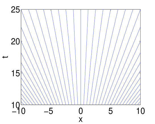
Figure 3: Lattice for the fundamental solution of the heat equation, $h=0.05$, $x_{0}=0$, $\tau=0.005$, $t_{0}=10$.

Another interesting solution that can be obtained is the traveling wave solution. This one is obtained by applying the symmetry transformation $\exp[c\mathbf{V}_{5}]$

$$\widetilde{u}=(a(\widetilde{x}-2c\widetilde{t})+b)\exp[-c\widetilde{x}+c^{2}\widetilde{t}],$$ (4tahbabtbxbzcba)

and is defined on the lattice

$$\widetilde{x}=hn+x_{0}+2c\widetilde{t},\qquad\widetilde{t}=\gamma(m).$$ (4tahbabtbxbzcbb)

By taking $\gamma(m)=\tau m+t_{0}$, we obtain a lattice in which the points in $x$ move linearly as a function of time.

4 Burgers’ equation

In this section we shall derive invariant schemes for the Burgers’ equation

$$v_{t}+vv_{x}=v_{xx}.$$ (4tahbabtbxbzcbcc)

This equation is well known to be related to the heat equation (4tag) by the Cole-Hopf transformation

$$v(x,t)=-2\frac{u_{x}(x,t)}{u(x,t)}.$$ (4tahbabtbxbzcbcd)

Since the transformation (4tahbabtbxbzcbcd) is not a point one, the symmetry algebras of the Burgers’ equation and the heat equation are not isomorphic. Indeed, the symmetry algebra of (4tahbabtbxbzcbcc) is five dimensional and is spanned by the vector fields [25]

$$\eqalign{\mathbf{V}_{1}=\partial_{x},\qquad\mathbf{V}_{2}=\partial_{t},\qquad\mathbf{V}_{3}=t\partial_{x}+\partial_{v},\\ \mathbf{V}_{4}=x\partial_{x}+2t\partial_{t}-v\partial_{v},\qquad\mathbf{V}_{5}=tx\partial_{x}+t^{2}\partial_{t}+(x-tv)\partial_{v}.}$$ (4tahbabtbxbzcbcg)

4.1 Invariant schemes

Before computing a set of fundamental discrete invariants let us mention the fact that the equation

$$T_{+}=0$$ (4tahbabtbxbzcbch)

is again weakly invariant under the group corresponding to (4tahbabtbxbzcbcg). The set of elementary invariants involving the same discrete points as for the heat equation (4tahau) is

$$\eqalign{I_{1}&=\frac{h_{+}}{h_{-}},\qquad\qquad I_{2}=\frac{\hat{h}_{+}}{\hat{h}_{-}},\qquad\qquad I_{3}=\frac{h_{+}\hat{h}_{+}}{\tau},\\ I_{4}&=h_{+}h_{-}(v^{+}_{x}-v_{x}^{-}),\qquad I_{5}=\hat{h}_{+}\hat{h}_{-}(\hat{v}^{+}_{x}-\hat{v}_{x}^{-}),\\ I_{6}&=h_{+}\Big{(}\frac{\sigma}{\tau}-v\Big{)},\qquad\quad\;\,I_{7}=\hat{h}_{+}\Big{(}\frac{\sigma}{\tau}-\hat{v}\Big{)},\\ I_{8}&=h_{+}^{2}\Big{(}v^{+}_{x}+\frac{1}{\tau}\Big{)},\qquad\;\;\;I_{9}=\hat{h}_{+}^{2}\Big{(}\hat{v}^{+}_{x}-\frac{1}{\tau}\Big{)},}$$ (4tahbabtbxbzcbcm)

where

$$v_{x}^{+}=\frac{v_{+}-v}{h_{+}},\qquad v_{x}^{-}=\frac{v-v_{-}}{h_{-}},\qquad\hat{v}_{x}^{+}=\frac{\hat{v}_{+}-\hat{v}}{\hat{h}_{+}},\qquad\hat{v}_{x}^{-}=\frac{\hat{v}-\hat{v}_{-}}{\hat{h}_{-}}.$$ (4tahbabtbxbzcbcn)

From the set of invariants (4tahbabtbxbzcbcm) and the weakly invariant equation (4tahbabtbxbzcbch) we derive invariant explicit and implicit schemes. The explicit scheme is obtained by putting

$$(2I_{6}-I_{7})I_{3}-I_{8}I_{6}=I_{4},\qquad T_{+}=0,\qquad I_{1}=1,$$ (4tahbabtbxbzcbco)

or in terms of the discrete variables

$$\bigg{(}2\Big{(}\frac{\sigma}{\tau}-v\Big{)}+\frac{\hat{h}}{h}\Big{(}\hat{v}-\frac{\sigma}{\tau}\Big{)}\bigg{)}\frac{\hat{h}}{h\tau}+\Big{(}v_{x}^{+}+\frac{1}{\tau}\Big{)}\Big{(}v-\frac{\sigma}{\tau}\Big{)}=\frac{v_{x}^{+}-v_{x}^{-}}{h},$$ (4tahbabtbxbzcbcpa)

$$T_{+}=0,$$ (4tahbabtbxbzcbcpb)

$$h_{+}=h_{-}\equiv h.$$ (4tahbabtbxbzcbcpc)

The implicit scheme is obtained by putting

$$(I_{6}-2I_{7})I_{3}-I_{9}I_{7}=I_{5},\qquad T_{+}=0,\qquad I_{2}=1,$$ (4tahbabtbxbzcbcpcq)

i.e.

$$\bigg{(}\frac{h}{\hat{h}}\Big{(}\frac{\sigma}{\tau}-v\Big{)}-2\Big{(}\frac{\sigma}{\tau}-\hat{v}\Big{)}\bigg{)}\frac{h}{\hat{h}\tau}-\Big{(}\frac{\sigma}{\tau}-\hat{v}\Big{)}\Big{(}\hat{v}_{x}^{+}-\frac{1}{\tau}\Big{)}=\frac{\hat{v}_{x}^{+}-\hat{v}_{x}^{-}}{h},$$ (4tahbabtbxbzcbcpcra)

$$T_{+}=0,$$ (4tahbabtbxbzcbcpcrb)

$$\hat{h}_{+}=\hat{h}_{-}\equiv\hat{h}.$$ (4tahbabtbxbzcbcpcrc)

As for the heat equation, the schemes generated involve $\hat{h}$ and $h$. Furthermore, the computation of the continuous limit of the invariant schemes (59) and (61) gives the same condition on the ratio $\sigma/\tau$ as for the heat equation, namely (4tahbabr). To see this, we compute the continuous limit of the explicit scheme (59). The calculation is similar for the implicit scheme (61). As for the heat equation, we suppose that the steps in $t$ and $x$ are given by (4tahbabj) and (4tahbabk), where we immediately assume that $k,l\geq 1$ in (4tahbabk) . First of all, it is clear that in the limit the equations specifying the lattice (4tahbabtbxbzcbcpb) and (4tahbabtbxbzcbcpc) go to the identity $0=0$. The development of (4tahbabtbxbzcbcpa) in a Taylor series in terms of the infinitesimal parameters $\epsilon$ and $\delta$ gives

$$\eqalign{\frac{\sigma}{\tau^{2}}+\frac{\sigma}{\tau}\left(\frac{\sigma_{+}-\sigma}{h\tau}\right)-\frac{v}{\tau}+\frac{\sigma}{\tau}v_{x}+v_{t}-v\left(\frac{\sigma_{+}-\sigma}{h\tau}\right)+v\left(\frac{\sigma_{+}-\sigma}{h\tau}\right)\\ -\frac{\sigma}{\tau}\left(\frac{\sigma_{+}-\sigma}{h\tau}\right)+vv_{x}-\frac{\sigma}{\tau}v_{x}+\frac{v}{\tau}-\frac{\sigma}{\tau^{2}}=v_{xx}+\Or(\epsilon^{2k-1},\epsilon^{2l-1},\delta).}$$ (4tahbabtbxbzcbcpcrcu)

In (4tahbabtbxbzcbcpcrcu) we have explicitely written all the terms that do not converge to zero in the limit, but after canceling the superfluous terms and making $\epsilon$ and $\delta$ go to zero we retrieve Burgers’ equation (4tahbabtbxbzcbcc).

In the particular case where the steps in $t$ are constant and $\sigma$ is zero, the invariant discretization reduces to standard one, namely

$$\frac{\hat{v}-v}{\tau}+vv_{x}^{+}=\frac{v_{x}^{+}-v_{x}^{-}}{h},$$

$$t=\tau m+t_{0},\qquad x=hx+x_{0},$$

for the explicit scheme and

$$\frac{\hat{v}-v}{\tau}+\hat{v}\hat{v}_{x}^{+}=\frac{\hat{v}_{x}^{+}-\hat{v}_{x}^{-}}{h},$$

$$t=\tau m+t_{0},\qquad x=hx+x_{0},$$

for the implicit one.

The invariant schemes just generated are closely related to those obtained by Dorodnitsyn and Kozlov [6]. The invariant schemes (59) and (61) are not uniquely defined, the discrete approximations of the Burgers’ equation (4tahbabtbxbzcbcpa) and (4tahbabtbxbzcbcpcra) can be defined on other lattices. For the explicit scheme we can replace (4tahbabtbxbzcbcpc) by the invariant equation

$$I_{6}=0.$$ (4tahbabtbxbzcbcpcrcv)

On this new lattice, (4tahbabtbxbzcbcpa) becomes

$$-I_{7}I_{3}=I_{4}.$$ (4tahbabtbxbzcbcpcrcw)

In terms of the variables $(x,t,v)$ we get the invariant explicit scheme

$$\eqalign{\frac{\hat{v}-v}{\tau}=\frac{h_{-}}{\hat{h}_{+}^{2}}(v_{x}^{+}-v_{x}^{-}),\\ T_{+}=0,\\ \sigma=\tau v.}$$ (4tahbabtbxbzcbcpcrda)

For the implicit symmetry-preserving scheme we can replace (4tahbabtbxbzcbcpcrc) by $I_{7}=0$ to obtain a scheme similar to those in [6]. In the case of the Burgers’ equation the invariant schemes in [6] can be seen as particular cases of the schemes we obtained. The major difference between the invariant schemes in [6] and (59) and (61) is that the steps in $x$ do not to have to be uniform in general.

4.2 Exact solutions

Similarly as for the heat equation, it is clear that the constant solution

$$v(x,t)=v_{0},$$ (4tahbabtbxbzcbcpcrdba)

defined on the orthogonal lattice

$$t_{m,n}=\gamma(m),\qquad x_{m,n}=hn+x_{0},$$ (4tahbabtbxbzcbcpcrdbb)

is an exact solution of the invariant schemes (59) and (61) ($v_{0}$, $h$ and $x_{0}$ are constants). By choosing $\gamma(m)=\tau m+t_{0}$ we get a standard rectangular lattice. Since the symmetry group of the Burgers’ equation is not very rich, just one new solution can be obtained from the constant one. By applying successively the symmetry transformations $\exp[\epsilon\mathbf{V}_{5}]$, $\exp[v_{0}/\epsilon\mathbf{V}_{1}]$ and $\exp[1/\epsilon\mathbf{V}_{2}]$ to (4tahbabtbxbzcbcpcrdba) and (4tahbabtbxbzcbcpcrdbb) we obtain

$$\widetilde{v}=\widetilde{x}/\widetilde{t}$$ (4tahbabtbxbzcbcpcrdbdca)

definied on the lattice

$$\widetilde{x}_{m,n}=\frac{\epsilon x_{m,n}+(1-\epsilon t_{m,n})v_{0}}{\epsilon(1-\epsilon t_{m,n})},\qquad\widetilde{t}_{m,n}=\frac{1}{\epsilon(1-\epsilon t_{m,n})}$$ (4tahbabtbxbzcbcpcrdbdcb)

If we choose $v_{0}=0$, take $\epsilon=1$ and pose $\gamma(m)=1-1/(\tau m+t)$ in (4tahbabtbxbzcbcpcrdbb), we conclude that the solution (4tahbabtbxbzcbcpcrdbdca) is an exact solution of the invariant schemes on the lattice

$$t_{m,n}=\tau m+t_{0},\qquad x_{m,n}=(hn+x_{0})(\tau m+t_{0}).$$ (4tahbabtbxbzcbcpcrdbdcdd)

The same lattice over which the fundamental solution of the heat equation is exact.

4.3 Burgers’ equation in potential form

The invariant discretization of the Burgers’ equation in potential form

$$w_{t}+\frac{(w_{x})^{2}}{2}=w_{xx}$$ (4tahbabtbxbzcbcpcrdbdcde)

is readily obtained from that of the linear heat equation. Indeed, since the PDE (4tahbabtbxbzcbcpcrdbdcde) is related to the heat equation (4tag) by the point transformation

$$u=\exp\left[-\frac{w}{2}\right],$$ (4tahbabtbxbzcbcpcrdbdcdf)

the results of Section 3 can directly be used to generate invariant schemes and exact solutions via the transformation (4tahbabtbxbzcbcpcrdbdcdf). For instance, the symmetry algebra of (4tahbabtbxbzcbcpcrdbdcde) is spanned by

$$\eqalign{\mathbf{V}_{1}=\partial_{x},\qquad\mathbf{V}_{2}=\partial_{t},\qquad\mathbf{V}_{3}=t\partial_{x}+x\partial_{w},\qquad\mathbf{V}_{4}=x\partial_{x}+2t\partial_{t},\\ \mathbf{V}_{5}=tx\partial_{x}+t^{2}\partial_{t}+(\frac{x^{2}}{2}+t)\partial_{w},\qquad\mathbf{V}_{6}=\partial_{w},}$$ (4tahbabtbxbzcbcpcrdbdcdgc)

$$\mathbf{V}_{\alpha}=\alpha(x,t)\exp\left[\frac{w}{2}\right]\partial_{w},$$ (4tahbabtbxbzcbcpcrdbdcdgd)

where $\alpha$ is a solution of the heat equation, $\alpha_{t}=\alpha_{xx}$.

4.3.1 Invariant schemes

Since the transformation (4tahbabtbxbzcbcpcrdbdcdf) does not affect the independant variables, it is clear that the equation (4tahat) is still a weakly invariant equation. We can directly use the set of elementary invariants (4tahay) and the transformation (4tahbabtbxbzcbcpcrdbdcdf) to obtain a set of elementary invariants on a flat time layer scheme [23]

$$\eqalign{I_{1}=\frac{h_{+}}{h_{-}},\qquad I_{2}=\frac{\hat{h}_{+}}{\hat{h}_{-}},\qquad I_{3}=\frac{h_{+}\hat{h}_{+}}{\tau},\qquad I_{4}=\frac{\sqrt{\tau}}{h_{+}}\exp\left[-\frac{\hat{w}-w}{2}+\frac{\sigma^{2}}{4\tau}\right]\\ I_{5}=\exp\left[-\frac{w_{+}-w}{2}+\frac{h_{+}}{4\tau}(2\sigma-h_{+})\right],\qquad I_{6}=\exp\left[\frac{w-w_{-}}{2}-\frac{h_{-}}{4\tau}(2\sigma+h_{-})\right],\\ I_{7}=\exp\left[-\frac{\hat{w}_{+}-\hat{w}}{2}+\frac{\hat{h}_{+}}{4\tau}(2\sigma+\hat{h}_{+})\right],\qquad I_{8}=\exp\left[\frac{\hat{w}-\hat{w}_{-}}{2}-\frac{\hat{h}_{-}}{4\tau}(2\sigma-\hat{h}_{+})\right].}$$ (4tahbabtbxbzcbcpcrdbdcdgdk)

By using the same invariant expressions (4tahaz) and (4tahbabb) we obtain invariant schemes for (4tahbabtbxbzcbcpcrdbdcde). An explicit scheme is

$$\eqalign{\frac{1}{\tau}\bigg{(}\sqrt{\frac{\hat{h}}{h}}\exp\left[-\frac{\hat{w}}{2}+\frac{\sigma^{2}}{4\tau}\right]-\exp\left[-\frac{w}{2}\right]\bigg{)}=\frac{1}{\hat{h}h}\bigg{(}\exp\left[-\frac{w_{+}}{2}+\frac{h}{4\tau}(2\sigma-h+\hat{h})\right]\\ -2\exp\left[-\frac{w}{2}\right]+\exp\left[\frac{w_{-}}{2}-\frac{h}{4\tau}(2\sigma+h-\hat{h})\right]\bigg{)},\\ T_{+}=0,\\ h_{+}=h_{-}\equiv h.}$$ (4tahbabtbxbzcbcpcrdbdcdgdp)

An implicit one is given by

$$\eqalign{\frac{1}{\tau}\bigg{(}\exp\left[-\frac{\hat{w}}{2}\right]-\sqrt{\frac{h}{\hat{h}}}\exp\left[-\frac{w}{2}-\frac{\sigma^{2}}{4\tau}\right]\bigg{)}=\frac{1}{\hat{h}h}\bigg{(}\exp\left[-\frac{w_{+}}{2}+\frac{\hat{h}}{4\tau}(2\sigma-h+\hat{h})\right]\\ -2\exp\left[-\frac{\hat{w}}{2}\right]+\exp\left[-\frac{\hat{w}_{-}}{2}-\frac{h}{4\tau}(2\sigma+h-\hat{h})\right]\bigg{)},\\ T_{+}=0,\\ \hat{h}_{+}=\hat{h}_{-}\equiv\hat{h}.}$$ (4tahbabtbxbzcbcpcrdbdcdgdu)

The invariant schemes (4tahbabtbxbzcbcpcrdbdcdgdp) and (4tahbabtbxbzcbcpcrdbdcdgdu) converge to the differential equation (4tahbabtbxbzcbcpcrdbdcde), if the condition (4tahbabr) on the lattice is satisfied. In contrast to the invariant schemes for the heat equation (32) and (4tahbabg), which give the standard discretization when $\sigma=0$; the invariant schemes (4tahbabtbxbzcbcpcrdbdcdgdp) and (4tahbabtbxbzcbcpcrdbdcdgdu) give unusual schemes on a rectangular lattice. For example, when $\sigma=0$ the explicit scheme (4tahbabtbxbzcbcpcrdbdcdgdp) becomes on a rectangular lattice

$$\eqalign{\frac{\exp\left[-\frac{\hat{w}}{2}\right]-\exp\left[-\frac{w}{2}\right]}{\tau}=\frac{\exp\left[-\frac{w_{+}}{2}\right]-2\exp\left[-\frac{w}{2}\right]+\exp\left[-\frac{w_{-}}{2}\right]}{h^{2}},\\ t=\tau m+t_{0},\qquad x=hn+x_{0},}$$ (4tahbabtbxbzcbcpcrdbdcdgdx)

which is quit different from the standard discretization

$$\frac{\hat{w}-w}{\tau}+\frac{1}{2}\left(\frac{w_{+}-w}{h}\right)^{2}=\frac{w_{+}-2w+w_{-}}{h^{2}}.$$

Finally, let us mention that the exact solutions obtained in Section 3.3 are mapped by (4tahbabtbxbzcbcpcrdbdcdf) to exact solutions of the invariant schemes (4tahbabtbxbzcbcpcrdbdcdgdp) and (4tahbabtbxbzcbcpcrdbdcdgdu). Since the transformation does not affect the independant variables the solutions obtained via (4tahbabtbxbzcbcpcrdbdcdf) are exact on the same lattice.

5 Korteweg-de Vries equation

As a last example, we consider the Korteweg-de Vries equation

$$u_{t}=uu_{x}+u_{xxx}.$$ (4tahbabtbxbzcbcpcrdbdcdgdy)

This equation has a four dimensional symmetry algebra spanned by

$$\mathbf{V}_{1}=\partial_{x},\qquad\mathbf{V}_{2}=\partial_{t},\qquad\mathbf{V}_{3}=t\partial_{x}-\partial_{u},\qquad\mathbf{V}_{4}=x\partial_{x}+3t\partial_{t}-2u\partial_{u}.$$ (4tahbabtbxbzcbcpcrdbdcdgdz)

5.1 Invariant schemes

Again, the equation (4tahat) is weakly invariant and we can discretize (4tahbabtbxbzcbcpcrdbdcdgdy) on a lattice with flat time layers. This time we make use of all points shown in figure 2 in order to approximate correctly the third order derivative in $x$. The usual computation gives the invariants

$$I_{1}=\frac{h_{+}}{h_{-}}, I_{2}=\frac{h_{++}}{h_{+}}, I_{3}=\frac{h_{-}}{h_{--}},$$

$$I_{4}=\frac{\hat{h}_{+}}{\hat{h}_{-}}, I_{5}=\frac{\hat{h}_{++}}{\hat{h}_{+}}, I_{6}=\frac{\hat{h}_{-}}{\hat{h}_{--}},$$

$$I_{7}=\frac{h_{+}}{\hat{h}_{+}}, I_{8}=\frac{h_{+}^{3}}{\tau}, I_{9}=\frac{\sigma+\tau u}{h_{+}},$$ (4tahbabtbxbzcbcpcrdbdcdgea)

$$I_{10}=\tau u_{x}^{--},\qquad I_{11}=\tau u_{x}^{-}, I_{12}=\tau u_{x}^{+},$$

$$I_{13}=\tau u_{x}^{++}, I_{14}=h_{+}^{2}(\hat{u}-u),\qquad I_{15}=\tau\hat{u}_{x}^{--},$$

$$I_{16}=\tau\hat{u}_{x}^{-}, I_{17}=\tau\hat{u}_{x}^{+}, I_{18}=\tau\hat{u}_{x}^{++},$$

with

$$u_{x}^{++}=\frac{u_{++}-u_{+}}{h_{++}},\quad u_{x}^{--}=\frac{u_{-}-u_{--}}{h_{--}},\quad\hat{u}_{x}^{++}=\frac{\hat{u}_{++}-\hat{u}_{+}}{\hat{h}_{++}},\quad\hat{u}_{x}^{--}=\frac{\hat{u}_{-}-\hat{u}_{--}}{\hat{h}_{--}}.$$ (4tahbabtbxbzcbcpcrdbdcdgeb)

An invariant explicit scheme approximating (4tahbabtbxbzcbcpcrdbdcdgdy) is obtained by putting

$$I_{14}=I_{9}I_{8}\frac{I_{12}-I_{11}}{2}+\frac{1}{2}(I_{13}-I_{12}-I_{11}+I_{10}),\qquad T_{+}=0,\qquad I_{1}=1.$$ (4tahbabtbxbzcbcpcrdbdcdgec)

In terms of the original variables we have

$$\frac{\hat{u}-u}{\tau}=u\frac{u_{+}-u_{-}}{2h}+\frac{u_{++}-2u_{+}+2u_{-}-u_{--}}{2h^{3}}+\frac{\sigma}{\tau}\frac{u_{+}-u_{-}}{2h},$$ (4tahbabtbxbzcbcpcrdbdcdgeda)

$$T_{+}=0,$$ (4tahbabtbxbzcbcpcrdbdcdgedb)

$$h_{+}=h_{-}\equiv h.$$ (4tahbabtbxbzcbcpcrdbdcdgedc)

Furthermore, an implicit scheme is obtained by considering the combination of invariants

$$I_{14}=(I_{9}+I_{8}^{-1}I_{14})I_{8}\frac{I_{17}-I_{16}}{2}+\frac{1}{2}(I_{18}-I_{17}-I_{16}+I_{15})I_{7}^{2},\quad T_{+}=0,\quad I_{4}=1,$$ (4tahbabtbxbzcbcpcrdbdcdgedee)

i.e.

$$\frac{\hat{u}-u}{\tau}=\hat{u}\frac{\hat{u}_{+}-\hat{u}_{-}}{2\hat{h}}+\frac{\hat{u}_{++}-2\hat{u}_{+}+2\hat{u}_{-}-\hat{u}_{--}}{2\hat{h}^{3}}+\frac{\sigma}{\tau}\frac{\hat{u}_{+}-\hat{u}_{-}}{2\hat{h}},$$ (4tahbabtbxbzcbcpcrdbdcdgedefa)

$$T_{+}=0,$$ (4tahbabtbxbzcbcpcrdbdcdgedefb)

$$\hat{h}_{+}=\hat{h}_{-}\equiv\hat{h}.$$ (4tahbabtbxbzcbcpcrdbdcdgedefc)

The invariant schemes include the standard discretizations. Indeed, if $\sigma$ equals zero then the last term on the right hand side of (4tahbabtbxbzcbcpcrdbdcdgeda) and (4tahbabtbxbzcbcpcrdbdcdgedefa) vanishes, which is just the usual discretization of the Korteweg-de Vries equation. In order for the equations (4tahbabtbxbzcbcpcrdbdcdgeda) and (4tahbabtbxbzcbcpcrdbdcdgedefa) to converge to (4tahbabtbxbzcbcpcrdbdcdgdy) the condition

$$\lim_{\tau\to 0}\frac{\sigma}{\tau}<\infty$$

must be imposed.

As for the Burgers’ equation, by considering the invariant schemes (81) and (83) on a lattice depending on the solution we recover similar schemes as those obtained in [4]. For the explicit scheme (81), if we replace (4tahbabtbxbzcbcpcrdbdcdgedc) by

$$I_{9}=0,$$ (4tahbabtbxbzcbcpcrdbdcdgedefeg)

the equation (4tahbabtbxbzcbcpcrdbdcdgeda) then becomes

$$I_{14}=\frac{1}{2}(I_{13}-I_{12}-I_{11}+I_{10}).$$ (4tahbabtbxbzcbcpcrdbdcdgedefeh)

In term of the variables $(x,t,u)$ we have

$$\eqalign{\frac{\hat{u}-u}{\tau}=\frac{(u_{x}^{++}-u_{x}^{+})-(u_{x}^{-}-u_{x}^{--})}{h_{+}^{2}},\\ T_{+}=0,\\ \sigma=-\tau u.}$$ (4tahbabtbxbzcbcpcrdbdcdgedefel)

For the implicit scheme (83) we just have to replace (4tahbabtbxbzcbcpcrdbdcdgedefc) by $I_{9}+I_{14}I_{8}^{-1}=0$ to get the invariant implicit scheme

$$\eqalign{\frac{\hat{u}-u}{\tau}=\frac{(\hat{u}_{x}^{++}-\hat{u}_{x}^{+})-(\hat{u}_{x}^{-}-\hat{u}_{x}^{--})}{\hat{h}_{+}^{2}}\\ T_{+}=0,\\ \sigma=-\tau\hat{u}.}$$ (4tahbabtbxbzcbcpcrdbdcdgedefep)

5.2 Exact solutions

As with all previously considered invariant schemes, the constant solution defined on an orthogonal mesh is an exact solution. Another exact solution of the invariant schemes corresponds to the solution invariant under the Galilei transformation generated by the vector field $\mathbf{V}_{3}$. This exact solution is obtained in a non-obvious fashion. The idea is the following one. Given the partial differential equation that we approximate, we can perform a symmetry reduction to obtain an exact solution $u(x,t)$. Given this solution, we can insert it in the discrete equation approximating the original differential equation, which will give an equation relating the independant variables. If the equation obtained can be solved using the existing liberty in the lattice, then we have generated an exact solution of the P$\Delta$S.

In the continuous case solution invariant under the infinitesimal symmetry generator $\mathbf{V}_{3}$ is

$$u=-\frac{x}{t}.$$ (4tahbabtbxbzcbcpcrdbdcdgedefeq)

By replacing this solution in (4tahbabtbxbzcbcpcrdbdcdgeda), we get

$$x=\frac{\sigma t}{\tau}.$$ (4tahbabtbxbzcbcpcrdbdcdgedefer)

If we take the evolution in time to be

$$t_{m,n}=\tau m+t_{0},$$ (4tahbabtbxbzcbcpcrdbdcdgedefes)

the equation (4tahbabtbxbzcbcpcrdbdcdgedefer) can be solved for $x$ and gives

$$x_{m,n}=(hn+x_{0})(\tau m+t_{0}).$$ (4tahbabtbxbzcbcpcrdbdcdgedefet)

Hence, we conclude that (4tahbabtbxbzcbcpcrdbdcdgedefeq) is an exact solution of the explicit scheme (81) on the lattice defined by the equations (4tahbabtbxbzcbcpcrdbdcdgedefes) and (4tahbabtbxbzcbcpcrdbdcdgedefet).

6 CONCLUSIONS

The discretization procedure presented in Section 2 and applied to specific examples in Section 3, 4 and 5 is a “minimal” one. By that we mean that the PDE (4j) is replaced by a P$\Delta$S (4n) involving only $N=3$ difference equations. The P$\Delta$S is by construction invariant under the symmetry group of the original PDE. The general solution of the P$\Delta$S (4n) will depend on several arbitrary functions of one (discrete) variable. A specific solution $u(x,t)$ and a specific lattice on which the solution is valid is obtained once these arbitrary functions are specified.

The freedom inherent in these arbitrary functions can be used in different ways. For instance, we can require that certain physically important solutions of the PDE should also be exact solutions of the P$\Delta$S. This was done in Section 3 with the fundamental solution of the heat equation.

An alternative possibility is to use the invariants of the symmetry group $G$ to add further invariant equations to the “minimal” P$\Delta$S (4n). This creates an overdetermined system of difference equations, restricting the freedom in the solutions. Since the system of $N$ equations with $N\geq 4$ is overdetermined, their compatibility must be assured. The idea of imposing an overdetermined system of invariant difference equations has already been explored earlier [3, 7, 15] with the aim of further restricting the form of the lattice.

All PDEs studied in this article are evolution equations of the form

$$u_{t}=f(x,t,u,u_{x},u_{xx},u_{xxx})$$ (4tahbabtbxbzcbcpcrdbdcdgedefeu)

and we made use of the fact that their symmetry groups always allowed horizontal time layers.

Other types of equations, requiring different lattices, will be studied in the future. The extension to more than one dependent variable and more than two independant ones is obvious.

This research program, “continuous symmetries of discrete equations” has both physical and mathematical aspects that must be further pursued. One conclusion is that different discrete physical systems require different approaches. It was shown elsewhere [12, 13] that symmetries of linear theories can be studied in terms of commuting difference operators on fixed lattices. The results of this and related papers [1, 2, 3, 4, 5, 6, 7, 8, 9, 10, 14, 15, 17, 21] indicate that at least for nonlinear discrete phenomena, the lattice should be considered as a dynamical one evolving together with the solution and described by an invariant system of difference equations.

From the mathematical point of view we see as the greatest challenge the development of symmetry adapted numerical schemes that give better results than standard numerical methods.

References

References

• [1] Bakirova M I, Dorodnitsyn V A and Kozlov R V 1997 Symmetry preserving difference schemes for some heat transfer equations J. Phys A. Math. Gen 30 8139–55
• [2] Budd C J and Dorodnitsyn V A 2001 Symmetry adapted moving mesh schemes for the nonlinear Schrödinger equation, J. Phys. A. Math. Gen. 34 10387–400
• [3] Dorodnitsyn V A 1991 Transformation groups in a space of difference variables J. Sov. Math. 55 1490–517
• [4] Dorodnitsyn V A 1994 Invariant discrete model for the Korteweg-de Vries equation Preprint CRM-2187, Université de Montréal
• [5] Dorodnitsyn V A 2001 Group properties of difference equations (Fizmatlit, Moscow) (in Russian)
• [6] Dorodnitsyn V A and Kozlov R 1997 The whole set of symmetry preserving discrete versions of a heat transfer equation with a source SYNODE, preprint Numerics No. 4
• [7] Dorodnitsyn V A and Kozlov R 2003 Heat transfer with a source: the complete set of invariant difference schemes J. Nonlin. Math. Phys 10 16–50
• [8] Dorodnitsyn V A, Kozlov R and Winternitz P 2000 Lie group classification of second order ordinary difference equations J. Math. Phys. 41 480–504
• [9] Dorodnitsyn V A, Kozlov R and Winternitz P 2004 Continuous symmetries of Lagrangians and exact solutions of discrete equations J. Math. Phys. 45 336–59
• [10] Dorodnitsyn V A and Winternitz P 2000 Lie point symmetry preserving discretizations for variable coefficient Korteweg-de Vries equations Nonlinear Dynamics 22 49–59
• [11] Floreanini R, Negro J, Nieto L M and Vinet L 1996 Symmetries of the heat equation on a lattice Lett. Math. Phys. 36 351–55
• [12] Levi D, Tempesta P and Winternitz P 2004 Lorentz and Galilei invariance on Lattices Phys. Rev. D 69 105011 pp. 1–6
• [13] Levi D, Tempesta P and Winternitz P 2004 Umbral calculus, difference equations and the discrete Schrödinger equation J. Math. Phys. 45 4077–105
• [14] Levi D, Tremblay S and Winternitz P 2000 Lie point symmetries of difference equations and lattices J. Phys. A Math. Gen. 33 8507–24
• [15] Levi D, Tremblay S and Winternitz P 2001 Lie symmetries of multidimensional equations and lattices J. Phys. A Math. Gen. 34 9507–24
• [16] Levi D, Vinet L and Winternitz P 1997 Lie group formalism for difference equations J. Phys. A Math. Gen. 30 633–49
• [17] Levi D and Winternitz P 1991 Continuous symmetries of discrete equations Phys. Lett. A 152 335–38
• [18] Levi D and Winternitz P 2004 Continuous symmetries of difference equations Preprint nlin.SI/0502004
• [19] Maeda S 1987 The similarity method for difference equations IMA J. Appl. Math. 38 129–34
• [20] Quispel G R W, Capel H W and Sahdevan R 1992 Continuous symmetries of difference equations: the Kac-van Morerbeke equation and the Painlevé reduction Phys. Lett. A 170 379–83
• [21] Rodriguez M A and Winternitz, P 2004 Lie symmetries and exact solutions of first-order difference schemes J. Phys. A Math. Gen. 37 6129–42
• [22] Valiquette F 2005 Discretizations preserving all Lie point symmetries of the Korteweg-de Vries equation Preprint math-ph/0507033
• [23] Valiquette F 2005 Point transformation in invariant difference schemes Preprint math-ph/0507041
• [24] Winternitz P 2004 Symmetries of discrete systems, in Discrete Integrable Systems, Lecture Notes in Physics 644, eds. Grammaticos B. Kossmann-Schwarzbach Y and Tamizhmani T (Springer, Berlin) 185–243
• [25] Olver P J 1993 Applications of Lie Groups to Differential Equations (Springer, New York)
• [26] Olver P J 1995 it Equivalence, Invariants, and Symmetries (Cambridge University Press, Cambridge)
• [27] Fels M and Olver P J 1998 Moving coframes I. A practical algorithm Acta Applic. Math. 51 161–213
• [28] Olver P J 2003 Moving frames J. Symb. Comp. 36 501–12