Estimates for moments of random matrices with Gaussian elements

Abstract

We describe an elementary method to get non-asymptotic estimates for the moments of Hermitian random matrices whose elements are Gaussian independent random variables. We derive a system of recurrent relations for the moments and the covariance terms and develop a triangular scheme to prove the recurrent estimates. The estimates we obtain are asymptotically exact in the sense that they give exact expressions for the first terms of $1/N$-expansions of the moments and covariance terms.

As the basic example, we consider the Gaussian Unitary Ensemble of random matrices (GUE). Immediate applications include the Gaussian Orthogonal Ensemble and the ensemble of Gaussian anti-symmetric Hermitian matrices. Finally we apply our method to the ensemble of $N\times N$ Gaussian Hermitian random matrices $H^{(N,b)}$ whose elements are zero outside of the band of width $b$. The other elements are taken from GUE; the matrix obtained is renormalized by $b^{-1/2}$. We derive the estimates for the moments of $H^{(N,b)}$ and prove that the spectral norm $\|H^{(N,b)}\|$ remains bounded in the limit $N,b\to\infty$ when $(\log N)^{3/2}/b\to 0$.

1 Introduction

The moments of $N\times N$ Hermitian random matrices $H_{N}$ are given by expression

$$M_{k}^{(N)}={\bf E}\left\{{1\over N}{\hbox{\ Tr}}\,(H_{N})^{k}\right\},$$

where ${\bf E}\{\cdot\}$ denotes the corresponding mathematical expectation. The asymptotic behavior of $M_{k}^{(N)}$ in the limit $N\to\infty$ is the source of numerous studies and vast list of publications. One can observe three main directions of researches; we list and mark them with the references that are earliest in the field up to our knowledge.

The first group of results is related with the limiting transition $N\to\infty$ when the numbers $k$ are fixed. In this case the limiting values of $M_{k}^{(N)}$, if they exist, determine the moments $m_{k}$ of the limiting spectral measure $\sigma$ of the ensemble $\{H_{N}\}$. This problem was considered first by E. Wigner [20].

Another asymptotic regime, when $k$ goes to infinity at the same time as $N$ does, is more informative and can be considered in two particular cases. In the first one $k$ grows slowly and $1\ll k\ll N^{\gamma}$ for any $\gamma>0$. In particular, if $k$ is of the order $\log N$ or greater, the maximal eigenvalue of $H_{N}$ dominates in the asymptotic behavior of $M_{2k}^{(N)}$. Then the exponential estimates of $M_{2k}^{(N)}$ provide the asymptotic bounds for the probability of deviations of the spectral norm $\|H_{N}\|$. This observation due to U. Grenander has originated a series of deep results started by S. Geman [1, 7, 9].

The second asymptotic regime is related to the limit when $k=O(N^{\gamma})$ with $\gamma>0$. The main subject here is to determine the critical exponent $\tilde{\gamma}$ such that the same estimates for $M_{2k}^{(N)}$ as in the previous case remain valid for all $\gamma\leq\tilde{\gamma}$ and fail otherwise [18]. This allows one to conclude about the order of the mean distance between eigenvalues at the border of the support of the limiting spectral density $d\sigma$ [4, 19].

In present article we describe a method to get the estimates of $M_{2k}^{(N)}$ that are valid for all values of $N$ and $k$ such that $k\leq CN^{\tilde{\gamma}}$ with some constant $C$. The estimates of this type are called non-asymptotic. However, they remain valid in the limit $N\to\infty$ and in this case they belong to the second asymptotic regime.

As the basic example, we consider the Gaussian Unitary (Invariant) Ensemble of random matrices that is usually abbreviated as GUE. In section 2 we describe our method and prove the main results for GUE. Immediate applications of our method include the Gaussian Orthogonal (Invariant) Ensemble of random matrices (GOE) and the Gaussian anti-symmetric (or skew-symmetric) Hermitian random matrices with independent elements. Detailed description of these ensembles is given in monograph [16]. In section 3 we present the non-asymptotic estimates for the corresponding moments.

Our approach is elementary. We use the integration by parts formula and generating functions technique only. We do not employ such a powerful methods like the orthogonal polynomials technique commonly applied to unitary and orthogonally invariant random matrix ensembles. This allows us to consider more general ensembles of random matrices than GUE and GOE. One of the possible developments is given by the study of the ensemble of Hermitian band random matrices $H^{(N,b)}$. The matrix elements of $H^{(N,b)}$ within the band of the width $b$ along the principal diagonal coincide with those of GUE. Outside of this band they are equal to zero; the matrix obtained is normalized by $b^{-1/2}$. In section 4 we prove non-asymptotic estimates for the moments of $H^{(N,b)}$. These estimates allow us to conclude about the asymptotic behavior of the spectral norm $\|H^{(N,b)}\|$ in the limit $b,N\to\infty$.

In section 5 we collect auxiliary computations and formulas used.

1.1 GUE, recurrent relations and semi-circle law

GUE is determined by the probability distribution over the set of Hermitian matrices $\{H_{N}\}$ with the density proportional to

$$\exp\{-2N{\hbox{\ Tr}}H_{N}^{2}\}.$$

The odd moments of $H_{N}$ are zero and the even ones $M_{2k}^{(N)}$ verify the following remarkable recurrent relation discovered by Harer and Don Zagier [11]

$$M_{2k}^{(N)}={2k-1\over 2k+2}\ M_{2k-2}^{(N)}+{2k-1\over 2k+2}\cdot{2k-3\over 2k}\cdot{k(k-1)\over 4N^{2}}\ M_{2k-4}^{(N)},$$

where $M_{0}^{(N)}=1$ and $M_{2}^{(N)}=1/4$. It follows from (1.2) that the moments $M_{2k}^{(N)},k=0,1,...$ converge as $N\to\infty$ to the limiting $m_{k}$ determined by relations

$$m_{k}={2k-1\over 2k+2}\ m_{k-1},\quad m_{0}=1.$$

The limiting moments $\{m_{k},k\geq 0\}$ are proportional to the Catalan numbers $C_{k}$:

$$m_{k}={1\over 4^{k}}{1\over(k+1)}{2k\choose k}={1\over 4^{k}}C_{k}$$

and therefore verify the following recurrent relation

$$m_{k}={\displaystyle 1\over\displaystyle 4}\ \sum_{j=0}^{k-1}\ m_{k-1-j}\ m_{j},\quad k=1,2,\dots$$

with obvious initial condition $m_{0}=1$.

In random matrix theory, equality (1.5) was observed for the first time by E. Wigner [20]. Relation (1.5) implies that the generating function of the moments $m_{k}$

$$f(\tau)=\sum_{k=0}^{\infty}\ m_{k}\cdot\tau^{k}$$

verifies quadratic equation $\tau f^{2}(\tau)-4f(\tau)+4=0$ and is given by

$$f(\tau)={1-\sqrt{1-\tau}\over\tau/2}.$$

Using (1.6), Wigner has shown that the measure $\sigma_{w}$ determined by the moments $m_{k}=\int\lambda^{2k}\ d\sigma_{w}(\lambda)$ has the density of the semicircle form

$$\sigma_{w}^{\prime}(\lambda)={2\over\pi}\cases{\sqrt{1-\lambda^{2}},&if $|\lambda|\leq 1$,\cr 0,&if $|\lambda|>1.$\cr}$$

The statement that the moments $M_{l}^{(N)}$ converge to $m_{k}$ for $l=2k$ and to $0$ for $l=2k+1$ is known as the Wigner semicircle law.

In present paper we show that the generating function $f(\tau)$ together with its derivatives represents a very convenient tool when estimating the moments $M_{2k}^{(N)}$. Everywhere below, we use denotation $[\cdot]_{k}$ for the $k$-th coefficient of the corresponding development, so $[f(\tau)]_{k}=m_{k}$.

1.2 Estimates for the moments of GUE

Using relations (1.2) and (1.3), one can easily prove by induction the estimate

$$M_{2k}^{(N)}\leq\left(1+{k^{2}\over 8N^{2}}\right)^{2k}\,m_{k}.$$

Indeed, let us assume inequalities $M_{2l}^{(N)}\leq(1+l^{2}/(gN^{2}))^{2l}m_{l}$ with some $g>0$ to hold for all values of $l$ such that $1\leq l\leq k-1$. Let us show that this is also true for $l=k$ provided $g\leq 8$.

Regarding the right-hand side of (1.2) and replacing $M_{2k-2}^{(N)}$ and $M_{2k-4}^{(N)}$ by corresponding estimates with $l=k-1$ and $l=k-2$, respectively, we bound the right-hand side of (1.2) by the sum of

$${2k-1\over 2k+2}\ \left(1+{(k-1)^{2}\over gN^{2}}\right)^{2k-2}m_{k-1}=\left(1+{(k-1)^{2}\over gN^{2}}\right)^{2k-2}m_{k}$$

and

$${k(k-1)\over 4N^{2}}\left(1+{(k-2)^{2}\over gN^{2}}\right)^{2k-4}m_{k}.$$

Here we have used identity (1.3). Comparing the expression obtained with the right-hand side of (1.8), we see that the following inequality

$$\left(1+{(k-1)^{2}\over gN^{2}}\right)^{2}+{k(k-1)\over 4N^{2}}\leq\left(1+{k^{2}\over gN^{2}}\right)^{4}$$

is sufficient for (1.8) to be true. Expanding the powers, we see that the condition $g\leq 8$ is sufficient to have (1.8) valid for all values of $k$ and $N$.

Estimates (1.8) are valid for all values of $k$ and $N$ without any restriction. They allow one to estimate the probability of deviations of the largest eigenvalue of $H_{N}$ (see, for example [14, 15] and references therein). Then one can study the asymptotic behavior of the maximal eigenvalues and also conclude about spectral scales at the borders of the support of $\sigma_{w}^{\prime}$ (see [18]).

It should be noted that relations (1.2) are obtained in [11] with the help of the orthogonal polynomials technique (see [10] and [15] for the simplified derivation). There are several more random matrix ensembles (see [15] for the references) whose moments verify recurrent relations of the type (1.2). But relations of the type (1.2) are rather exceptional than typical. Even in the case of GOE, it is not known whether relations of the type (1.2) exist. As a result, no simple derivation of the estimates of the form (1.8) for GOE has been reported.

We develop one more approach to prove non-asymptotic estimates of the type (1.8). Instead of relations (1.2), we use the system of recurrent relations (1.5) that is of more general character than (1.2). Regarding various random matrix ensembles, one can observe that the limiting moments verify either (1.5) by itself or one or another system recurrent relations generalizing (1.5) (see for instance, section 5 of [3], where the first elements of the present approach were presented).

We derive a system of recurrent relations for the moments $M_{2k}^{(N)}$ that have (1.5) as the limiting form. These relations for $M_{2k}^{(N)}$ involve corresponding covariance terms. Using the generation functions technique, we find the form of estimates and use the triangle scheme of the recurrent estimates to prove the bounds for moments and covariance terms. The final result can be written as

$$M_{2k}^{(N)}\leq\left(1+\alpha{k^{3}\over N^{2}}\right)m_{k}$$

with some $\alpha>1/12$. The estimates obtained are valid in the domain $k^{3}\leq\chi N^{2}$ with some constant $\chi$, i.e. not for all values of $k$ and $N$, as (1.8) does. But in this region our estimates are more precise than those of (1.8). If $k^{3}\ll N^{2}$, our estimates provide exact expressions for $1/N$-corrections for the moments $M_{2k}^{(N)}$.

1.3 Band random matrices and the semi-circle law

Hermitian band random matrices $H^{(N,b)}$ can be obtained from GUE matrices by erasing all elements outside of the band of width $b$ along the principal diagonal and by renormalizing the matrix obtained by the factor $b^{-1/2}$. It appears that the limiting values of the moments

$$M_{2k}^{(N,b)}={\bf E}\left\{{1\over N}{\hbox{\ Tr}}\left(H^{(N,b)}\right)^{2k}\right\}$$

crucially depend of the ratio between $b$ and $N$ when $N\to\infty$ (see [5, 13, 17]).

If $b/N\to 1$ as $N\to\infty$, then $M_{2k}^{(N,b)}\to m_{k}$ and the semicircle law is valid in this case. If $b/N\to c$ and $0<c<1$, then the limiting values of $M_{2k}^{(N,b)}$ differ from $m_{k}$. Finally, if $1\ll b\ll N$, then the semicircle law is valid again.

The last asymptotic regime of (relatively) narrow band width attracts a special interest of researchers. In this case the spectral properties of band random matrices exhibit a transition from one type to another. The first one is characterized by GUE matrices and the second is given by spectral properties of Jacobi random matrices, i.e. the discrete analog of the random Schrödinger operator with $b=3$ (see [6, 8] for the results and references). It is shown that the value $b^{\prime}=\sqrt{N}$ is critical with respect to this transition [6, 8, 12].

In present paper we derive the estimates for $M^{(N,b)}_{2k}$ that have the same form as the estimates for GUE with $N$ replaced by $b$. This can be viewed as an evidence to the fact that the asymptotic behavior of the eigenvalues of $H^{(N,b)}$ at the border of the semi-circle density is similar to that of matrices of the size $b\times b$. The estimates we obtain show that the value $b^{\prime}=\sqrt{N}$ does not play any particular role with respect to the asymptotic behavior of the spectral norm $\|H^{(N,b)}\|$. We show that if $b\gg(\log N)^{3/2}$, then the spectral norm converges with probability 1 when $N\to\infty$ to the edge of the corresponding semicircle density. Up to our knowledge, this is the first result on the upper bound of the spectral norm of band random matrices.

2 Gaussian Hermitian Ensembles

Let us consider the family of complex random variables

$$h_{xy}=\cases{V_{xy}+{\hbox{ i}}W_{xy},&if $x\leq y$,\cr V_{yx}-{\hbox{ i}}W_{yx},&if $x>y$,\cr}$$

where $\{V_{xy},W_{xy},\ 1\leq x\leq y\leq N\}$ are real jointly independent random variables that have normal (Gaussian) distribution with the properties

$${\bf E}V_{xy}={\bf E}W_{xy}=0,$$

and

$${\bf E}V_{xy}^{2}=({1+\delta_{xy}}){1+\eta\over 8}\,,\quad{\bf E}W_{xy}^{2}=({1-\delta_{xy}}){1-\eta\over 8}\,,$$

where $\delta_{xy}$ is the Kronecker $\delta$-symbol and $\eta\in[-1,1]$. Then we obtain the family of Gaussian ensembles of $N\times N$ Hermitian random matrices of the form

$$(H_{N}^{(\eta)})_{xy}={1\over\sqrt{N}}\,h_{xy},\quad x,y=1,\dots,N$$

that generalizes the Gaussian Unitary Ensemble (1.1). Indeed, it is easy to see that $\{H^{(0)}_{N}\}$ coincides with the GUE, while $\{H^{(1)}\}$ and $\{H^{(-1)}\}$ reproduce the GOE and Hermitian skew-symmetric Gaussian matrices. In [16], the last ensemble is referred to as the Hermitian anti-symmetric one; below we follow this terminology. The present section is devoted to the results for GUE and their proofs. Two other ensembles will be considered in the section 3.

2.1 Main results for GUE and the scheme of the proof

Let us consider the moments $M_{2k}^{(N)}$ of GUE matrices. We prove a little more precise estimate than (1.9).

Theorem 2.1

Given any constant $\alpha>1/12$, there exists $\chi>0$ such that the estimate

$$M_{2k}^{(N)}\leq\left(1+\alpha{k(k^{2}-1)\over N^{2}}\right)m_{k}$$

holds for all values of $k,N$ under condition that $k^{3}/N^{2}\leq\chi$.

Remark. Using relation (1.2), one can prove (2.4) under condition that

$$\alpha>{1\over 12-\chi}.$$

This relation shows that Theorem 2.1 gives the correct lower bound for $\alpha$. In our proof we get relations between $\chi$ and $\alpha$ more complicated than (2.5), but they are of the same character as (2.5). It follows from (2.5) that the closer $\alpha$ to $1/12$ is, the smaller $\chi$ has to be chosen and vice versa. Indeed, the following proposition shows that the estimate (2.4) is asymptotically exact.

Theorem 2.2

Given $k$ fixed, the following asymptotic expansion holds,

$$M_{2k}^{(N)}=m_{k}+{1\over N^{2}}m_{k}^{(2)}+O(N^{-4}),\quad{\hbox{as }}N\to\infty,$$

where

$$m_{k}^{(2)}={k(k-1)(k+1)\over 12}\ m_{k},\quad k\geq 1.$$

If $k\to\infty$ and $\tilde{\chi}=k^{3}/N^{2}\to 0$, then relation (2.6a) remains true with $O(N^{-4})$ replaced by $o(\tilde{\chi})$.

Remark. It follows from (1.2) that the sequence $\{m_{k}^{(2)},k\geq 1\}$ is determined by recurrent relation

$$m_{k}^{(2)}={2k-1\over 2k+2}\cdot m_{k-1}^{(2)}+{k(k-1)\over 4}\cdot m_{k},\quad k=1,2,\dots$$

with obvious initial condition $m^{(2)}_{0}=0$. It is easy to check that (2.6b) is in complete agreement with this recurrent relation for $m_{k}^{(2)}$.

Let us explain the role of recurrent relations (1.5) in the proof of Theorem 2.1. To do this, let us consider the normalized trace $L_{a}={1\over N}\,{\hbox{\ Tr}}\,H^{a}$

$${\bf E}\{L_{a}\}={1\over N}\sum_{x,s=1}^{N}{\bf E}\{H_{xs}H^{a-1}_{sx}\}$$

and compute the last mathematical expectation. Here and below we omit subscripts and superscripts $N$ when no confusion can arise. Applying the integration by parts formula (see section 5 for details), we obtain equality

$${\bf E}\{L_{a}\}={1\over 4}\sum_{j=0}^{a-2}{\bf E}\{L_{a-2-j}L_{j}\}.$$

Introducing the centered random variables $L^{o}_{j}=L_{j}-{\bf E}L_{j}$, we can write that

$${\bf E}\left\{L_{a_{1}}L_{a_{2}}\right\}={\bf E}\{L_{a_{1}}\}\,{\bf E}\{L_{a_{2}}\}+{\bf E}\{L^{o}_{a_{1}}L^{o}_{a_{2}}\}.$$

Taking into account that ${\bf E}L_{2k+1}=0$, we deduce from (2.7) relation

$$M_{2k}^{(N)}={1\over 4}\sum_{j=0}^{k-1}M_{2k-2-2j}^{(N)}\,M_{2j}^{(N)}+{1\over 4}\ D_{2k-2}^{(2;N)},$$

where we denoted

$$D_{2k-2}^{(2;N)}=\sum_{a_{1}+a_{2}=2k-2}{\bf E}\{L^{o}_{a_{1}}L^{o}_{a_{2}}\}.$$

Obviously, the last summation runs over $a_{i}>0$. Comparing (2.8) with (1.5), we see that the problem is to estimate the covariance terms $D^{(2)}$. Here and below we omit superscripts $N$ when no confusion can arise.

In what follows, we prove that under conditions of Theorem 2.1,

$$|D^{(2;N)}_{2k}|\leq{ck\over N^{2}},$$

with some constant $c$. Inequality (2.9) represents the main technical result of this paper. It is proved in the next subsection. With (2.9) in hands, we can use relation (2.8) to show that (2.4) holds.

Now let us explain the use of the generating function $f(\tau)$ (1.6). Regarding the right-hand side of (2.4), one can observe that the third derivative of $f(\tau)$ could be useful in computations because of the equality $[f^{\prime\prime\prime}(\tau)]_{k}=(k+3)(k+2)(k+1)m_{k+3}$. Indeed, more accurate computations (see identity (5.12) of section 5) show that the function

$$f(\tau)+{A\over N^{2}}{\tau^{2}\over(1-\tau)^{5/2}}=\Phi_{N}(\tau)\quad\hbox{with}\quad A={3\alpha\over 4}$$

is a very good candidate to generate the estimating expressions. This is not by a simple coincidence or an artificial choice. Later we will see that the form of $\Phi_{N}(\tau)$ is in certain sense optimal. It is dictated by the iteration scheme we use to get $1/N$-corrections for the moments and covariance terms (see subsection 2.5, the proof of Theorem 2.2).

Let us now show how (2.9) implies the estimate

$$M_{2k}^{(N)}\leq\left[\Phi_{N}(\tau)\right]_{k}.$$

Assuming that this estimates and (2.9) are valid for all the terms of the right-hand side of (2.8), we can estimate it with the help of inequalities

$${1\over 4}\sum_{j=0}^{k-1}M_{2k-2-2j}M_{2j}+{1\over 4}|D^{(2)}_{2k-2}|\leq{1\over 4}\left[\Phi^{2}_{N}(\tau)\right]_{k-1}+{c\over 4N^{2}}\left[{1\over(1-\tau)^{2}}\right]_{k-2}.$$

Denoting by $\Theta(k;N)$ the terms of the order $O(N^{-4})$, we can write that

$$\left[{\tau\over 4}\Phi^{2}_{N}(\tau)\right]_{k}=\left[{\tau f^{2}(\tau)\over 4}+{\tau^{3}f(\tau)\over 2}{A\over N^{2}(1-\tau)^{5/2}}\right]_{k}+\Theta(k;N).$$

Rewriting (1.6) and quadratic equation for $f(\tau)$ in convenient forms

$${\tau f^{2}(\tau)\over 4}=f(\tau)-1\quad{\hbox{and}}\quad{\tau f(\tau)\over 2}=1-\sqrt{1-\tau},$$

we transform the expression in the brackets:

$$\left[f(\tau)+{A\over N^{2}}{\tau^{2}\over(1-\tau)^{5/2}}-{A\over N^{2}}{\tau^{2}\over(1-\tau)^{2}}\right]_{k}=\left[\Phi_{N}(\tau)\right]_{k}-{A\over N^{2}}\left[{\tau^{2}\over(1-\tau)^{2}}\right]_{k}.$$

Remembering that $[\Phi_{N}(\tau)]_{k}$ reproduces the expression to estimate $M_{2k}^{(N)}$, we conclude that (2.10) is valid provided

$${A\over N^{2}}\left[{\tau^{2}\over(1-\tau)^{2}}\right]_{k}\geq{c\over 4N^{2}}\left[{\tau^{2}\over(1-\tau)^{2}}\right]_{k}={c(k-1)\over 4N^{2}}.$$

This requires inequality $A\geq c/4$.

The final comment is related to the role of the terms $\Theta(k;N)$. They are of the form

$$\Theta(k;N)={A^{2}\over 4N^{4}}\left[{\tau^{5}\over(1-\tau)^{5}}\right]_{k}\leq{A^{2}k^{4}\over N^{4}}.$$

If one wants these terms not to violate inequality (2.12) involving terms of the form $k/N^{2}$, one has to set the ratio $k^{3}/N^{2}=\tilde{\chi}$ sufficiently small. This explains the last condition of Theorem 2.1.

It should be noted that the same comments concern the proof of the estimate of covariance terms (2.9), where the recurrent relations, generating functions and terms of the type $\tilde{\chi}$ appear. In the proofs, we constantly use relations (2.11).

2.2 Main technical result

In this subsection we prove the estimates of the covariance terms of the type $D^{(2)}_{2k}=\sum{\bf E}\{L_{a_{1}}^{o}L^{o}_{a_{2}}\}$. The main idea is that these terms are determined by a system of recurrent relations similar to (2.8). These relations involve the terms of more complicated structure than $D^{(2)}$. The variables we study are defined as

$$D^{(q)}_{2k}=\sum_{a_{1}+\dots+a_{q}=2k}D^{(q)}_{a_{1},\dots,a_{q}}={\sum_{a_{1}+\dots+a_{q}=2k}}{\bf E}\left\{L^{o}_{a_{1}}L^{o}_{a_{2}}\cdots L^{o}_{a_{q}}\right\},\quad q\geq 2.$$

Here and everywhere below, we assume that the summation runs over all positive integers $a_{i}>0$. Our main technical result is given by the following statement.

Proposition 2.1.

Given $A>1/16$, there exists $\chi>0$ such that estimate (2.10) holds for all values of $1\leq k\leq k_{0}$, where $k_{0}$ verifies condition

$${k_{0}^{3}\over N^{2}}\leq\chi\ .$$

Also there exists $C$

$${1\over 24}<C<\max\{{2A\over 3},4!\}$$

such that inequalities

$$|D_{2k}^{(2s)}|\leq C{(3s)!\over N^{2s}}\left[{\tau\over(1-\tau)^{2s}}\right]_{k},$$

and

$$|D_{2k}^{(2s+1)}|\leq C{(3s+3)!\over N^{2s+2}}\left[{\tau\over(1-\tau)^{2s+5/2}}\right]_{k},$$

are true for all $k,s$ such that

$$2k+q\leq 2k_{0}$$

with $q=2s$ and $q=2s+1$, respectively.

Remark. The form of estimates (2.15) is dictated by the structure of the recurrent relations we derive below. The bounds for the constants $A$ and $C$ and of the form factorial terms of (2.15) are explained in subsection 2.4.

We prove Proposition 2.1 in the next subsection on the base of recurrent relations for $D^{(q)}$ that we derive now. Let us use identity for centered random variables ${\bf E}\{X^{o}Y^{o}\}={\bf E}\{XY^{o}\}$ and consider equality

$${\bf E}\left\{L^{o}_{a_{1}}L^{o}_{a_{2}}\cdots L^{o}_{a_{q}}\right\}={\bf E}\left\{L_{a_{1}}[L^{o}_{a_{2}}\cdots L^{o}_{a_{q}}]^{o}\right\}={1\over N}\sum_{x,s=1}^{N}{\bf E}\left\{H_{xs}(H^{a_{1}-1}_{sx}[L^{o}_{a_{2}}\cdots L^{o}_{a_{q}}]^{o}\right\}$$

We apply to the last expression the integration by parts formula (5.1) and obtain equality

$$D^{(q)}_{a_{1},\dots,a_{q}}={1\over 4}\sum_{j=0}^{a_{1}-2}{\bf E}\left\{L_{a_{1}-2-j}L_{j}[L^{o}_{a_{2}}\cdots L^{o}_{a_{q}}]^{o}\right\}$$

$$+{1\over 4N^{2}}\sum_{i=2}^{q}{\bf E}\left\{L^{o}_{a_{2}}\cdots L^{o}_{a_{i-1}}\ a_{i}\ L_{a_{i}+a_{1}-2}L^{o}_{a_{i+1}}\dots L^{o}_{a_{q}}\right\},$$

with the help of formulas (5.7) and (5.8), respectively. The detailed derivation of (2.18) is presented in subsection 5.2.

Let us consider the first term from the right-hand side of (2.18). We can rewrite it in terms of variables $D$ with the help of the following identity

$${\bf E}\{L_{1}L_{2}Q^{o}\}={\bf E}\{L_{1}\}{\bf E}\{L_{2}^{o}Q\}+{\bf E}\{L_{2}\}{\bf E}\{L_{1}^{o}Q\}+{\bf E}\{L_{1}^{o}L_{2}^{o}Q\}-{\bf E}\{L_{1}^{o}L_{2}^{o}\}{\bf E}\{Q\},$$

where $Q=L_{a_{2}}^{o}\cdots L_{a_{q}}^{o}$. Regarding the last term of (2.18), we use (2.17) and obtain relation

$$D^{(q)}_{a_{1},\dots,a_{q}}={1\over 4}\sum_{j=0}^{a_{1}-2}M_{j}D^{(q)}_{a_{1}-2-j,a_{2},\dots,a_{q}}+{1\over 4}\sum_{j=0}^{a_{1}-2}M_{a_{1}-2-j}D^{(q)}_{j,a_{2},\dots,a_{q}}$$

$$+{1\over 4}\sum_{j=0}^{a_{1}-2}D^{(q+1)}_{j,a_{1}-2-j,a_{2},\dots,a_{q}}-{1\over 4}\sum_{j=0}^{a_{1}-2}D^{(2)}_{j,a_{1}-2-j}D^{(q-1)}_{a_{2},\dots,a_{q}}$$

$$+{1\over 4N^{2}}\sum_{i=2}^{q}a_{i}M_{a_{1}+a_{i}-2}D^{(q-2)}_{a_{2},\dots,a_{i-1},a_{i+1},\dots,a_{q}}+{1\over 4N^{2}}\sum_{i=2}^{q}a_{i}D^{(q-1)}_{a_{2},\dots,a_{i-1},a_{i}+a_{1}-2,a_{i+1},\dots,a_{q}}.$$

Taking into account that $M_{2k+1}^{(N)}=0$, it is easy to deduce from (2.19) by induction on $k$ that

$$D_{a_{1},\dots,a_{q}}^{(q)}=0\quad\hbox{whenever}\ \ a_{1}+\dots+a_{q}=2k+1.$$

Let us introduce variables

$$\bar{D}^{(q)}_{2k}=\sum_{a_{1}+\dots+a_{q}=2k}\left|D^{(q)}_{a_{1},\dots,a_{q}}\right|.$$

Using the positivity of $M_{2j}$, we derive from (2.19) the second main relation

$$\bar{D}_{2k}^{(q)}\leq{1\over 2}\sum_{j=0}^{k-1}\bar{D}^{(q)}_{2k-2-2j}M_{2j}+{q-1\over 4N^{2}}\sum_{j=0}^{k-1}\bar{D}_{2k-2-2j}^{(q-2)}\cdot{(2j+2)(2j+1)\over 2}\cdot M_{2j}$$

$$+{1\over 4}\bar{D}^{(q+1)}_{2k-2}+{1\over 4}\sum_{j=0}^{k-1}\bar{D}^{(q-1)}_{2k-2-2j}\bar{D}^{(2)}_{2j}+{2k(2k-1)\over 2}\cdot{(q-1)\over 4N^{2}}\cdot\bar{D}_{2k-2}^{(q-1)},$$

where $1\leq k,2\leq q\leq 2k$. When regarding two last terms of (2.19), we have used obvious equality

$$\sum_{a_{1}+a_{2}=a^{\prime}}a_{2}\ F_{a_{1}+a_{2}-2}=\left(\sum_{a_{2}=1}^{a^{\prime}-1}a_{2}\right)F_{a^{\prime}-2}={a^{\prime}(a^{\prime}-1)\over 2}F_{a^{\prime}-2}.$$

Using this relation with $F$ replaced by $M$ and $a^{\prime}=2j+2$, we obtain that

$$\sum_{a_{1}+\dots+a_{q}=2k}a_{i}M_{a_{1}+a_{i}-2}|D^{(q)}_{a_{1},\dots,a_{i-1},a_{i+1},\dots,a_{q}}|=\sum_{j=0}^{k-1}\bar{D}_{2k-2-2j}^{(q-2)}{(2j+2)(2j+1)\over 2}\cdot M_{2j}.$$

Also we can write that

$$\sum_{a_{1}+\dots+a_{q}=2k}a_{i}|D^{(q-1)}_{a_{2},\dots,a_{i-1},a_{i}+a_{1}-2,a_{i+1},\dots,a_{q}}|$$

$$=\sum_{b_{2}+\dots+b_{q}=2k-2}|D^{(q-1)}_{b_{2},\dots,b_{q}}|\times\sum_{1\leq a_{1}\leq b_{i}+1}(b_{i}-a_{1}+2)\leq\sum_{a_{1}+\dots+a_{q-1}=2k-2}|D^{(q-1)}_{a_{1},\dots,a_{q-1}}|\times{2k(2k-1)\over 2}$$

and get the last term of (2.20).

The upper bounds of sums in (2.20) are written under agreement that $\bar{D}_{2k}^{(q)}=0$ whenever $q>2k$. Also we note that the form of inequalities (2.20) is slightly different when we consider particular values of $q$ and $k$. Indeed, some terms are missing when the left-hand side is $\bar{D}^{(2)}_{2k}$, $\bar{D}^{(3)}_{2k}$, $\bar{D}^{(2k)}_{2k}$, $\bar{D}^{(2k-1)}_{2k}$, and $\bar{D}^{(2k-2)}_{2k}$. However, the agreement that $\bar{D}_{2k}^{(q)}=0$ whenever $q>2k$ and that $\bar{D}^{(1)}_{2k}=0$ and $\bar{D}^{(0)}_{2k}=\delta_{k,0}$ make (2.20) valid in these cases.

Obviously, we have that

$$M_{2k}\leq{1\over 4}\sum_{j=0}^{k-1}M_{2k-2-2j}\,M_{2j}+{1\over 4}\bar{D}_{2k-2}^{(2)}.$$

2.3 Recurrent relations and estimates

To estimate $M$ and $\bar{D}^{(q)}$, we introduce auxiliary numbers $B_{k}^{(N)}\geq 0$ and $R^{(q;N)}_{2k}\geq 0$ determined by a system of two recurrent relations induced by (2.20) and (2.21). This system is given by the following equalities (we omit superscripts $N$)

$$B_{k}={1\over 4}\left(B*B\right)_{k-1}+{1\over 4}R_{k-1}^{(2)},$$

and

$$R_{k}^{(q)}={1\over 2}\left(R^{(q)}*B\right)_{k-1}+{q-1\over 4N^{2}}\left(R^{(q-2)}*B^{\prime\prime}\right)_{k-1}+{1\over 4}R^{(q+1)}_{k-1}$$

$$+{1\over 4}\left(R^{(q-1)}*R^{(2)}\right)_{k-1}+{k^{2}q\over 2N^{2}}R_{k-1}^{(q-1)},$$

considered in the domain

$$\Delta=\{(k,q):\ k\geq 1,\,2\leq q\leq 2k\}$$

with denotation

$$B^{\prime\prime}_{k}={(2k+2)(2k+1)\over 2}B_{k}$$

and the convolutions as follows

$$\left(B*B\right)_{k-1}=\sum_{j=0}^{k-1}B_{k-1-j}B_{j}.$$

The initial values for (2.22)-(2.23) coincide with those of $M$ and $D$:

$$B_{0}^{(N)}=1,\ \quad R_{1}^{(2;N)}={1\over 4N^{2}}.$$

Let us note that one can consider relations (2.22) and (2.23) for all integers $k$ and $q$ with obvious agreement that outside of $\Delta$ the values of $R$ are zero except the origin $R^{(0;N)}_{0}=1$. The system (2.22)-(2.23) plays a fundamental role in our method the proof of Proposition 2.1. This proof is composed of the following three statements.

Lemma 2.1.

Given fixed $N$, the family of numbers $\{B_{k},R^{(q)}_{k},\ (k,q)\in\Delta\}$ exist; it is uniquely determined by the system of relations (2.22)-(2.23).

Lemma 2.2.

Inequalities

$$M_{2k}^{(N)}\leq B_{k}^{(N)}\quad{\hbox{and }}\quad\bar{D}^{(q;N)}_{2k}\leq R^{(q;N)}_{k}$$

hold for all $N$ and $(k,q)\in\Delta$.

Lemma 2.3.

Under conditions of Proposition 2.1, the numbers $B_{k}$ and $R^{(q)}_{k}$ are estimated by the right-hand sides of inequalities (2.10), (2.14) and (2.15), respectively; that is

$$B_{k}^{(N)}\leq\left[f(\tau)+AN^{-2}\tau^{2}(1-\tau)^{-5/2}\right]_{k}\equiv[\Phi_{N}(\tau)]_{k}$$

and

$$R^{(q;N)}_{k}\leq\cases{C(3s)!N^{{-2s}}\left[\tau(1-\tau)^{-2s}\right]_{k},&if $q=2s$;\cr C(3s+3)!N^{-2s-2}\left[\tau(1-\tau)^{-(4s+5)/2}\right]_{k},&if $q=2s+1$.\cr}$$

Lemma 2.3 represents the main technical result concerning the system (2.22)-(2.23). Lemmas 2.1 and 2.2 looks like a simple consequence of the recurrent procedure applied to relations (2.22)-(2.23) and (2.20)-(2.21), respectively. However, the form of recurrent relations (2.22)-(2.23) is not usual because relations for $B$ involve the values of $R$ and vice-versa. The ordinary scheme of recurrence has to be modified. This modification is described in the next subsection. Lemma 2.3 is also proved on the base of this modified scheme of recurrence.

2.3.1 The triangular scheme of recurrent estimates

Let us show on the example of Lemma 3 that the ordinary scheme of recurrent estimates can be applied to the system (2.20)-(2.23). Under the ordinary scheme we mean the following reasoning. Assume that the estimates we need are valid for the terms entering the right-hand side of the inequalities derived. Apply these estimates to all terms there and show that the sum of the expressions obtained is smaller than that we assume for the terms of the left-hand side; check the estimates of the initial terms. Then all estimates we need are true. Let consider the plane of integers $(k,q)$ assume that estimates (2.26) are valid for all variables $R$ with $(k,q)$ lying inside of the triangle domain $\Delta(m),m\geq 3$

$$\Delta(m)=\{(k,q):\ 1\leq k,\,2\leq q\leq 2k,\,k+q\leq m\}$$

and that estimates (2.25) are valid for all variables $B_{l}$ with $1\leq l\leq m-2$.

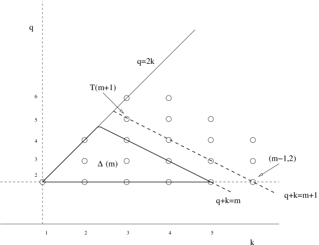
Figure 1: The triangle domain $\Delta(m)$ with $m=7$ and the long dotted line $k+q=m+1$

Then we proceed to complete the next line $k+q=m+1$ step by step starting from the top point $T(m+1)$ of $\Delta(m+1)$ and ending at the bottom point $(m-1,2)$ of this side line. This means that on each step, we assume estimates (2.25) and (2.26) valid for all terms entering the right-hand sides of relations (2.23) and show that the same estimate is valid for the term standing at the left hand side of (2.23).

Once the bottom point $(m-1,2)$ achieved, we turn to relation (2.22) and prove that estimate (2.25) is valid for $B_{m}$. Again, this is done by assuming that all terms entering the right-hand side of (2.22) verify estimates (2.25) and (2.26) with $q=2$, and showing that the expression obtained is bounded by the right-hand side of (2.25). This completes the triangular scheme of recurrent estimates.

It is easy to see that the reasoning described above proves, with obvious changes, Lemmas 2.1 and 2.2.

2.3.2 Estimates for $B$

Assuming that the terms standing in the right-hand side of (2.22) are estimates (2.25) and (2.26) with $s=1$, we can write inequality

$${1\over 4}(B*B)_{k-1}+{1\over 4}R_{k-1}^{(2)}$$

$$\leq\left[{\tau f^{2}(\tau)\over 4}+{A\over N^{2}}{\tau^{3}f(\tau)\over 2(1-\tau)^{5/2}}+{A^{2}\over 4N^{4}}{\tau^{5}\over(1-\tau)^{5}}\right]_{k}+{3C\over 2N^{2}}\left[{\tau^{2}\over(1-\tau)^{2}}\right]_{k}.$$

Taking into account relations (2.11), we transform the first bracket of (2.27) into expression

$$\left[f(\tau)+{A\over N^{2}}{\tau^{2}\over(1-\tau)^{5/2}}\right]_{k}-{A\over N^{2}}\left[{\tau^{2}\over(1-\tau)^{2}}\right]_{k}+{A^{2}\over 4N^{4}}\left[{\tau^{5}\over(1-\tau)^{5}}\right]_{k}.$$

Here, the first term reproduces expression $[\Phi_{N}(\tau)]_{k}$ ; the second term is negative and this allows us to show that the estimate wanted is true. Then we see that estimate $B_{k}\leq[\Phi_{N}(\tau)]_{k}$ is true whenever inequality

$$A\left[{\tau^{2}\over(1-\tau)^{2}}\right]_{k}\geq{3C\over 2}\left[{\tau^{2}\over(1-\tau)^{2}}\right]_{k}+{A^{2}\over 4N^{2}}\left[{\tau^{5}\over(1-\tau)^{5}}\right]_{k}$$

holds. This is equivalent to the condition

$$A\geq{3C\over 2}+{A^{2}\over 4N^{2}}{(k-4)(k-3)(k-2)\over 4!}.$$

Remembering that $k^{3}\leq\chi N^{2}$, we see that the estimate (2.25) of $B_{k}$ is true provided

$$A\geq{3C\over 2}+{A^{2}\chi\over 96}.$$

2.3.3 Estimates for $R^{(2s)}$

Let us rewrite (2.8) with $q=2s,s\geq 2,\ k\geq 1$ in the form

$$R_{k}^{(2s)}={1\over 2}\left(R^{(2s)}*B\right)_{k-1}+{2s-1\over 4N^{2}}\left(R^{(2s-2)}*B^{\prime\prime}\right)_{k-1}+X+Y+Z,$$

where we denoted

$$X={1\over 4}R^{(2s+1)}_{k-1},\quad Y={1\over 4}\left(R^{(2s-1)}*R^{(2)}\right)_{k-1},\quad Z={k^{2}s\over N^{2}}R_{k-1}^{(2s-1)}.$$

The first term in the right-hand side of (2.30) admits the following estimate

$${1\over 2}\left(R^{(2s)}*B\right)_{k-1}\leq{C(3s)!\over N^{2s}}\left[{\tau^{2}f(\tau)\over 2(1-\tau)^{2s}}+{A\over 2N^{2}}{\tau^{4}\over(1-\tau)^{2s+5/2}}\right]_{k}.$$

Using (2.11), we transform the last expression to the form

$${C(3s)!\over N^{2s}}\left[{\tau\over(1-\tau)^{2s}}-{\tau\over(1-\tau)^{2s-1/2}}+{A\over 2N^{2}}{\tau^{4}\over(1-\tau)^{2s+5/2}}\right]_{k}.$$

The first term reproduces the expression we need to estimate $R^{(2s)}_{k}$.

Let us consider the second terms of the right-hand side of (2.30). Assuming (2.25) and using identities of subsection 5.1, it is not hard to show that

$$B_{k}^{\prime\prime}\leq\left[{1\over(1-\tau)^{3/2}}+{18A\over N^{2}}{1\over(1-\tau)^{9/2}}\right]_{k}.$$

Indeed, it follows from (5.11) that

$${(2k+2)(2k+1)\over 2}[f(\tau)]_{k}={(2k+2)(2k+1)\over 2}m_{k}=\left[{1\over(1-\tau)^{3/2}}\right]_{k}.$$

Next, identity (5.12) implies relation

$${(2k+2)(2k+1)\over 2}\left[{\tau^{2}\over(1-\tau)^{5/2}}\right]_{k}={(2k+2)(2k+1)\over 2}\cdot{2k(2k-1)(2k+1)\over 3!}m_{k}.$$

Now, regarding (5.9) with $r=4$, it is easy to see that

$$\left[{1\over(1-\tau)^{9/2}}\right]_{k}={(2k+1)(2k+2)(2k+3)(2k+5)(2k+7)\over 5\cdot 6\cdot 7}m_{k}.$$

Then (2.33) follows.

Returning to the right-hand side of (2.30), we can write with the help of (2.33) inequality

$$\left(R^{(2s-2)}*B^{\prime\prime}\right)_{k-1}\leq{C(3s-3)!\over 4N^{2s-2}}\left[{\tau\over(1-\tau)^{2s-1/2}}+{18A\over N^{2}}{\tau\over(1-\tau)^{2s+5/2}}\right]_{k}.$$

Here and below we use relation $[\tau^{j}g(\tau)]_{k}\leq[g(\tau)]_{k}$ valid for the generating functions under consideration. Let us stress that (2.34) remains valid in the case of $s=1$ with $C$ replaced by $1$.

Let us turn to (2.31). We estimate the sum of $X$ and $Y$ by

$$X+Y\leq{C(1+C)(3s+3)!\over 4N^{2s+2}}\left[{\tau\over(1-\tau)^{2s+5/2}}\right]_{k}\ .$$

For the last term of (2.31) we can write inequality

$$Z\leq{Ck^{2}(3s+1)!\over N^{2s+2}}\left[{\tau\over(1-\tau)^{2s+1/2}}\right]_{k}\ .$$

Comparing the second term of (2.32) with the sum of the last term of (2.32) and the right-hand sides of (2.34), (2.35), and (2.37), we arrive at the following inequality to hold

$$C\geq{(2s-1)(3s-3)!\over(3s)!}\cdot{\delta_{s,1}+C(1-\delta_{s,1})\over 4}+{k^{2}(3s+1)\over 3N^{2}}\cdot{\left[\tau(1-\tau)^{-2s-1/2}\right]_{k}\over\left[\tau(1-\tau)^{-2s+1/2}\right]_{k}}\$$

$$+C{(1+C)(3s+3)!+18A(3s-2)!+2A(3s)!\over 4N^{2}(3s)!}\cdot{\left[\tau(1-\tau)^{-2s-5/2}\right]_{k}\over\left[\tau(1-\tau)^{-2s+1/2}\right]_{k}}\ .$$

Using identity (5.10), we see that

$${\left[\tau(1-\tau)^{-2s-1/2}\right]_{k}\over\left[\tau(1-\tau)^{-2s+1/2}\right]_{k}}={2k+4s-2\over 4s-1}\leq{4k_{0}\over 4s-1}.$$

Similarly

$${\left[\tau(1-\tau)^{-2s-5/2}\right]_{k}\over\left[\tau(1-\tau)^{-2s+1/2}\right]_{k}}\ \leq{(4k_{0})^{3}\over(4s-1)(4s+1)(4s+3)}.$$

Inserting these inequalities into (2.37),maximizing the expressions obtained with respect to $s$, and using (2.13), we get the following sufficient condition

$$C\geq{\delta_{s,1}+C(1-\delta_{s,1})\over 24}+2\chi\,\left(1+10C(1+C)+2AC\right).$$

2.3.4 Estimates for $R^{(2s+1)}$

Let us turn to the case $q=2s+1$ and rewrite (2.8) in the form

$$R_{k}^{(2s+1)}={1\over 2}\left(R^{(2s+1)}*B\right)_{k-1}+{s\over 2N^{2}}\left(R^{(2s-1)}*B^{\prime\prime}\right)_{k-1}+X_{1}+Y_{1}+Z_{1},$$

where

$$X_{1}={1\over 4}R^{(2s+2)}_{k-1},\quad Y_{1}={1\over 4}\left(R^{(2s-1)}*R^{(2)}\right)_{k-1},\ Z_{1}={k^{2}s\over N^{2}}R_{k-1}^{(2s)}.$$

Regarding the first term of (2.39), we can write inequality

$${1\over 2}\left(R^{(2s+1)}*B\right)_{k}\leq{C(3s+3)!\over N^{2s+2}}\left[{\tau^{2}f(\tau)\over 2(1-\tau)^{2s+5/2}}+{A\tau\over 2N^{2}(1-\tau)^{2s+5}}\right]_{k}$$

$$={C(3s+3)!\over N^{2s+2}}\left[{\tau\over(1-\tau)^{2s+5/2}}-{\tau\over(1-\tau)^{2s+2}}+{A\tau\over 2N^{2}(1-\tau)^{2s+5}}\right]_{k}\ .$$

The first term of the right-hand side of (2.41) reproduces the expression needed to estimate $R^{(2s+1)}_{k}$.

Let us consider the second term of (2.39). It is estimated as follows:

$${s\over 2N^{2}}\left(R^{(2s-1)}*B^{\prime\prime}\right)_{k-1}\leq{Cs(3s)!\over 2N^{2s+2}}\left[{\tau\over(1-\tau)^{2s+2}}\right]_{k}+{9ACs(3s)!\over N^{2s+4}}\left[{\tau\over(1-\tau)^{2s+5}}\right]_{k}\ .$$

Regarding two first terms of (2.40), we can write that

$$X_{1}+Y_{1}\leq{C(3s+3)!+6C^{2}(3s)!\over 4N^{2s+2}}\left[\tau\over(1-\tau)^{2s+2}\right]_{k},$$

and

$$Z_{1}\leq{Ck^{2}s(3s)!\over N^{2s+2}}\left[{\tau\over(1-\tau)^{2s}}\right]_{k}.$$

Comparing the negative term of (2.41) with the sum of the last term of (2.41) and the estimates for the terms of (2.40), we obtain inequality

$$C\left({3\over 4}-{s(3s)!\over 2(3s+3)!}\right)\geq{3C^{2}(3s)!\over 2(3s+3)!}+{k^{2}s(3s)!\over(3s+3)!}\cdot{[\tau(1-\tau)^{-2s}]_{k}\over[\tau(1-\tau)^{-2s-2}]_{k}}\$$

$$+{AC\over 2N^{2}}\cdot\left(1+{18s(3s)!\over(3s+3)!}\right)\cdot{[\tau(1-\tau)^{-2s-5}]_{k}\over[\tau(1-\tau)^{-2s-2}]_{k}}.$$

Equality (5.13) implies that

$${[\tau(1-\tau)^{-2s}]_{k}\over[\tau(1-\tau)^{-2s-2}]_{k}}\ ={2s(2s+1)\over(k-1+2s)(k+2s)}$$

and that

$${[\tau(1-\tau)^{-2s-5}]_{k}\over[\tau(1-\tau)^{-2s-2}]_{k}}\leq{8k_{0}^{3}\over(2s+2)(2s+3)(2s+4)}.$$

Inserting these two relations into (2.42) and maximizing expressions with respect to $s$, we obtain, after elementary transformations, the following sufficient condition

$$C\leq{4!\over 1+4A\chi}.$$

2.4 Proof of Theorem 2.1

Let us repeat that inequalities (2.29), (2.38), and (2.43) represent sufficient conditions for recurrent estimates (2.25) and (2.26) to be true. Let $A>1/16$. Then for any constant $C<4!$ verifying condition

$${1\over 24}<C<{2A\over 3},$$

there exists such $\chi>0$ that (2.38) is true. Indeed, it is sufficient to take $\chi\leq\chi^{\prime}$, where $\chi^{\prime}$ is such that

$$2\chi^{\prime}K<\min\{C-{1\over 24},{23\over 24}C\},$$

with $K=1+10C(1+C)+2AC$. Also there exists $\chi^{\prime\prime}$ such that (cf. (2.29))

$$A\geq 3C/2+A^{2}\chi^{\prime\prime}.$$

The choice of $\chi\leq\min\{\chi^{\prime},\chi^{\prime\prime}\}$ makes (2.29) and (2.38) true. Condition (2.43) is obviously verified. Thus, conditions (2.13), (2.14), and $A>1/16$ of Proposition 2.1 are sufficient for (2.29), (2.38), and (2.43) to hold. This completes the proof of Lemma 2.3.

Lemma 2.2 together with Lemma 2.3 implies estimates (2.10) and (2.15). Then Proposition 2.1 follows. The statement of Theorem 1.1 is a simple consequence of the estimate (2.10) and Proposition 2.1.

We complete this subsection with the discussion of the form of estimates (2.26) and constants $A$ and $C$. First let us note that the upper bound $4!$ for $C$ imposed by (2.14) represents a technical restriction; it can be avoided, for example, by modifying estimates (2.26) for $R^{(2s)}$ and $R^{(2s+1)}$, where $C$ is replaced by $C^{s}$ and $C^{s+1}$, respectively. However, in this case the lower bounds $1/16$ for $A$ and $1/24$ for $C$ are to be replaced by $1/6$ and $1/9$, respectively.

The closer $A$ and $C$ to optimal values $1/16$ and $1/24$ are, the smaller $\chi$ is to be chosen. The inverse is also correct. Namely, in the next subsection we prove that estimates (2.9) and (2.10) become asymptotically exact in the limit $\chi\to 0$. In this case factorials $(3s)!$ and $(3s+3)!$ in the right-hand sides of (2.26) can be replaced by other expressions $g(s)$ and $h(s)$ that provide more precise estimates for $R^{(q)}$. Indeed, repeating the computations of subsections 2.3.3 and 2.3.4, one can see that in the limit $\chi\to 0$ function $g(s)$ can be chosen close to $(2s-1)!!/4^{s}$. This make an evidence for the central limit theorem to hold for the centered random variables

$$NL_{a}^{o}={\hbox{\ Tr}}\,H^{a}-{\bf E}\{{\hbox{\ Tr}}\,H^{a}\}.$$

This observation explains also the fact that the odd ”moments” of the variable $L^{o}_{a}$ decrease faster than the even ones as $N\to\infty$. That is why the estimates for $R^{(2s)}$ have the form different from those of $R^{(2s+1)}$ and are proved separately.

For finite values of $\chi$, the use of some expression proportional to $(3s)!$ is unavoidable.

2.5 Proof of Theorem 2.2

We present the proof of Theorem 2.2 for the case when $k$ is fixed and $N\to\infty$. Regarding relation (2.19) with $q=2$, we obtain relation

$$D^{(2)}_{2k}={1\over 2}\left(D^{(2)}*M\right)_{2k-2}+{1\over 4N^{2}}\cdot{2k(2k-1)\over 2}M_{2k-2}+{1\over 4}D^{(3)}_{2k-2}.$$

Proposition 2.1 implies that $D^{(3)}_{2k}=O(N^{-4})$ and that $M_{2k}^{(N)}-m_{k}=O(N^{-2})$. Then we easily arrive at the conclusion that

$$D^{(2)}_{2k}={r_{k}\over N^{2}}+O\left({1\over N^{4}}\right),$$

where $r_{k}$ are determined by relations $r_{0}=0$ and

$$r_{k}={1\over 2}\left(r*m\right)_{k-1}+{1\over 4}\cdot{2k(2k-1)\over 2}m_{k-1},\quad k\geq 1.$$

Passing to the generating functions and using relations (2.11) and (5.11), we obtain equality

$$r_{k}={1\over 4}\left[{\tau\over(1-\tau)^{2}}\right]_{k}={k\over 4}.$$

Returning to relation (2.8), we conclude that

$$M_{2k}^{(N)}=m_{k}+{1\over N^{2}}m_{k}^{(2)}+O\left({1\over N^{4}}\right).$$

Indeed, the difference between $M_{2k}^{(N)}$ and $m_{k}$ is of the order $N^{-2}$ and the next correction is of the order $N^{-4}$. Regarding $m_{k}^{(2)}$ and using (2.45), we obtain equality

$$m_{k}^{(2)}={1\over 2}\left[m^{(2)}*m\right]_{k-1}+{1\over 16}\left[{\tau^{2}\over(1-\tau)^{2}}\right]_{k},\quad k\geq 1,$$

and $m_{1}^{(2)}=0$. Solving (2.47) with the help of (2.11), we get expression

$$m_{k}^{(2)}={1\over 16}\left[{\tau^{2}\over(1-\tau)^{5/2}}\right]_{k}.$$

It is easy to see that (2.48) implies relation

$${1\over 16}\left[{\tau^{2}\over(1-\tau)^{5/2}}\right]_{k}={1\over 16}{(2k-3)(2k-2)(2k-1)\over 3!}m_{k-2}$$

and hence (2.6b). Theorem 2.2 is proved.

2.6 More about asymptotic expansions

The system (2.22)-(2.23) of recurrent relations is the main technical tool in the proof of the Proposition 2.1, where the estimates for $B$ and $R$ are given. However, the crucial question is to find the correct form of these estimates. The first terms of the asymptotic expansions described in previous subsection give a solution of this problem. Indeed, repeating the proof of Theorem 2.2, we see that formulas (2.46) and (2.48) indicate the form of the estimates to be proved. Then the proof of Proposition 2.1 is reduced to elementary computations, where the most important part is related with the correct choice of the factorial terms in inequalities (2.15).

The next observation is that relation (2.23) resembles inequality (2.20) obtained from (2.19) by considering the absolute values of variables $D^{(q)}_{a_{1},\dots,a_{q}}$ and replacing in the right-hand side of (2.19) the sign ”$-$” by the sign ”+”. So, relation (2.23) determine the estimating terms $R^{(q)}$ with certain error. However, it is not difficult to deduce from estimates (2.25) and (2.26) that if $q=2s$, then this error is of the order smaller than the order of $R^{(2s)}$. This means that relations (2.23) determine correctly the first terms of the $1/N$-expansions of all $R^{(2s)},s\geq 1$ and not only of $R^{(2)}$ as mentioned by Theorem 2.2. The same is true for the $1/N$ expansions of $D^{(2s)}_{2k}$. It is easy to show by using (2.23) and results of Proposition 2.1 that these corrections are given by formulas

$$D^{(2s)}_{2k}=r^{(2s)}_{k}+o(k^{2s-1}/N^{2s}),$$

where $r^{(2s)}_{k}$ are such that the corresponding generating function $\tilde{r}^{(2s)}(\tau)=\sum_{k\geq 0}r^{(2s)}_{k}\tau^{k}$ verifies equation

$$\tilde{r}^{(2s)}(\tau)={\tau f(\tau)\over 2}\tilde{r}^{(2s)}(\tau)+(2s-1)\tilde{r}^{(2s-2)}(\tau){d^{2}\over 2N^{2}d\tau^{2}}(\tau f(\tau)).$$

Using equalities (2.11) and resolving (2.49), we obtain expression

$$\quad r^{(2s)}_{k}={(2s-1)!!\over(4N^{2})^{s}}\left[{\tau^{s}\over(1-\tau)^{2s}}\right]_{k}.$$

The left-hand side of relation (2.23) for $R^{(q)}_{k}$ involves variables $R^{(q)}_{j}$, $R^{(q-1)}_{j}$, and $R^{(q+1)}$. This can lead one to the idea to use the generating functions of two variables $G(\tau,\mu)$ to describe the family of numbers $R$. In this connection, the following comment on the structure of the variables $D^{(q)}$ could be useful. Introducing a generating function $F(\tau)=\sum_{j\geq 0}\tau^{j}L_{j}$, we see that

$$\sum_{k\geq 1}D^{(q)}_{2k}\tau^{2k}={\bf E}\{[F^{o}(\tau)]^{q}\},$$

where $F^{o}(\tau)=F(\tau)-{\bf E}F(\tau)$. Then the mentioned above function can have the form

$$G_{D}(\tau,\mu)=\sum_{k\geq 1,q\geq 2}D^{(q)}_{2k}\tau^{2k}{\mu^{q}\over q!}={\bf E}\left\{e^{\mu F^{o}(\tau)}\right\}-1.$$

In particular, regarding such a generating function of $r^{(2s)}_{k}$, one arrives at the expression

$$G_{r}(\tau,\mu)=\sum_{k\geq 1,s\geq 1}r^{(2s)}_{k}\tau^{2k}{\mu^{2s}\over(2s)!}=\exp\left\{{\mu^{2}\over 4N^{2}}{\tau\over(1-\tau)^{2}}\right\}.$$

This expression show that the central limit theorem can be proved for the random variable $NF^{o}(\tau)$ in the asymptotic regime $k^{3}/N^{2}\ll 1$ mentioned in Theorem 2.2. This asymptotic regime can be compared with the mesoscopic regime for the resolvent of $H_{N}$ and the central limit theorem valid there [2].

3 Orthogonal and anti-symmetric ensembles

In this section we return to Hermitian random matrix ensembles $H^{(\eta)}$ with $\eta=1$ and $\eta=-1$ introduced in section 2. Let us consider the moments of $H^{(1)}$. Using the method developed in section 2, we prove the following statements.

Theorem 3.1 (GOE).

Given $A>1/2$, there exists $\chi$ such that

$$M_{2k}^{(N)}\leq m_{k}+A{1\over N}$$

for all $k,N$ such that $k\leq k_{0}$ and (2.13) hold. If $k$ is fixed and $N\to\infty$, then

$$M_{2k}^{(N)}=m_{k}+{1-(k+1)m_{k}\over 2N}+o(N^{-1})$$

and

$$D^{(2;N)}_{2k}=\sum_{a+b=2k}{\bf E}\left\{L_{a}^{o}L_{b}^{o}\right\}={k\over 2N^{2}}+O(N^{-3}).$$

The proof of Theorem 3.1 is obtained by using the method described in section 2. Briefly saying, we derive recurrent inequalities for $M_{2k}^{(N)}$ and $D^{(q)}_{2k}$, then introduce related auxiliary numbers $B$ and $R$ determined by a system of recurrent relations. Using the triangular scheme of recurrent estimates to prove the estimates we need. Corresponding computations are somehow different from those of section 2. We describe this difference below (see subsection 3.1).

Let us turn to the ensemble $H^{(-1)}$. Regarding the recurrent relations for the moments of these matrices, we will see that for $M_{2k}^{(\eta=-1)}$ are bounded by $M_{2k}^{(\eta=1)}$. Slightly modifying the computations performed in the proof of Theorem 3.1, one can prove the following result.

Theorem 3.2 (Gaussian anti-symmetric Hermitian matrices).

Given $A>1/2$, there exists $\chi>0$ such that the moments of Gaussian skew-symmetric Hermitian ensemble $H^{(-1)}_{N}$ admit the estimate

$$M_{2k}^{(N)}\leq m_{k}+A{1\over N}$$

for all values of $k,N$ such that (2.13) holds. Also

$$|D^{(2)}_{2k}|=O\left({1\over N^{2}}\right)\quad\hbox{and}\quad|D^{(3)}_{2k}|=O\left({1\over N^{3}}\right).$$

Given $k$ fixed, the following asymptotic expansions are true for the moments of $H^{(-1)}$

$$M^{(N)}_{2k}=m_{k}+{\delta_{k,0}-(k+1)m_{k}\over 2N}+o(N^{-1}),$$

and for the covariance terms

$$D^{(2;N)}_{2k}=\sum_{a_{1}+a_{2}=2k}{\bf E}\left\{L^{o}_{a_{1}}L^{o}_{a_{2}}\right\}={k+1\over 4N^{2}}+O(N^{-3}).$$

3.1 Proof of Theorem 3.1

Using the integration by parts formula (5.7) with $\eta=1$ and repeating computations of the previous section, we obtain recurrent relation for $M_{2k}={\bf E}L_{2k}$;

$$M_{2k}={1\over 4}\sum_{j=0}^{k-1}M_{2k-2-2j}M_{2j}+{2k-1\over 4N}M_{2k-2}+{1\over 4}\sum_{a_{1}+a_{2}=2k-2}{\bf E}\left\{L_{a_{1}}^{o}L_{a_{2}}^{o}\right\}.$$

Regarding the variables

$$D^{(q)}_{2k}=\sum_{a_{1},\dots,a_{q}}^{2k}D^{(q)}_{a_{1},\dots,a_{q}}=\sum_{a_{1},\dots,a_{q}}^{2k}{\bf E}\left\{L^{o}_{a_{1}}L^{o}_{a_{2}}\cdots L^{o}_{a_{q}}\right\}$$

and using formulas (5.6) and (5.8) with $\eta=1$, we obtain relation

$$D^{(q)}_{a_{1},\dots,a_{q}}={1\over 4}\sum_{j=0}^{a_{1}-2}M_{j}D^{(q)}_{a_{1}-2-j,a_{2},\dots,a_{q}}+{1\over 4}\sum_{j=0}^{a_{1}-2}M_{a_{1}-2-j}D^{(q)}_{j,a_{2},\dots,a_{q}}$$

$$+{1\over 4}\sum_{j=0}^{a_{1}-2}D^{(q+1)}_{j,a_{1}-2-j,a_{2},\dots,a_{q}}-{1\over 4}\sum_{j=0}^{a_{1}-2}D^{(2)}_{j,a_{1}-2-j}D^{(q-1)}_{a_{2},\dots,a_{q}}+{1\over 4N}(a_{1}-1){\bf E}\left\{L_{a_{1}-2}^{o}L_{a_{2}}^{o}\cdots L_{a_{q}}^{o}\right\}$$

$$+{1\over 2N^{2}}\sum_{i=2}^{q}a_{i}M_{a_{1}+a_{i}-2}D^{(q-2)}_{a_{2},\dots,a_{i-1},a_{i+1},\dots,a_{q}}+{1\over 2N^{2}}\sum_{i=2}^{q}a_{i}D^{(q-1)}_{a_{2},\dots,a_{i-1},a_{i}+a_{1}-2,a_{i+1},\dots,a_{q}}.$$

Introducing variables

$$\bar{D}^{(q)}_{2k}=\sum_{a_{1},\dots,a_{q}}^{2k}\left|{\bf E}\left\{L_{a_{1}}^{o}\cdots L_{a_{q}}^{o}\right\}\right|,$$

we derive from (3.9) inequality

$$\bar{D}_{2k}^{(q)}\leq{1\over 2}\sum_{j=0}^{k-1}\bar{D}^{(q)}_{2k-2-2j}M_{2j}+{1\over 4}\bar{D}^{(q+1)}_{2k-2}+{1\over 4}\sum_{j=0}^{k-1}\bar{D}^{(q-1)}_{2k-2-2j}\bar{D}^{(2)}_{2j}+{k\over 2N}\bar{D}^{(q)}_{2k-2}$$

$$+{q-1\over 2N^{2}}\sum_{j=0}^{k-1}\bar{D}^{(q-2)}_{2k-2-2j}{(2j+2)(2j+1)\over 2}M_{2j}+{(q-1)k^{2}\over N^{2}}\cdot\bar{D}_{2k-2}^{(q-1)}.$$

We have used here the same transformations as it was used when passing from equality (2.19) to inequality (2.20).

Now we proceed as in Section 2 and introduce the auxiliary numbers $B$ and $R$ that verify relations

$$B_{k}={1\over 4}\left(B*B\right)_{k-1}+{k\over 2N}B_{k-1}+{1\over 4}R^{(2)}_{k-1},\quad k\geq 1,$$

and

$$R^{(q)}_{k}={1\over 2}\left(B*R^{(q)}\right)_{k-1}+{q-1\over 2N^{2}}\left(B^{\prime\prime}*R^{(q-2)}\right)_{k-1-j}$$

$$+{k\over 2N}R_{k-1}^{(q)}+{1\over 4}R^{(q+1)}_{k-1}+{1\over 4}\left(R^{(2)}*R^{(q-1)}\right)_{k-1}+{qk^{2}\over N^{2}}R_{k-1}^{(q-1)}.$$

The initial conditions are: $B_{0}=1$, $R_{1}^{(2)}=1/(2N^{2})$. The triangular scheme of recurrent estimates implies inequalities

$$M_{2k}^{(N)}\leq B_{k}^{(N)},\quad{\hbox{and}}\quad|D_{2k}^{(q)}|\leq\bar{D}^{(q)}_{2k}\leq R_{k}^{(q)}.$$

The main technical result for GOE is given by the following proposition.

Proposition 3.1

Let us consider $B$ and $R$ for the case of GOE ($\eta=1$). Given $A>1/2$ and $1/4<C<2\cdot 6!$, there exists $\chi$ such that the following estimates

$$B^{(N)}_{k}\leq m_{k}+{A\over N},\quad k\geq 2,$$

or equivalently

$$B^{(q)}_{k}\leq\left[f(\tau)\right]_{k}+{A\over N}\left[{\tau\over 1-\tau}\right]_{k},\quad k\geq 2,$$

and

$$R^{(2s)}_{k}\leq{C(3s)!\over N^{2s}}\left[{\tau\over(1-\tau)^{2s}}\right]_{k},$$

and

$$R^{(2s+1)}_{k}\leq{C(3s+3)!\over N^{2s+2}}\left[{\tau\over(1-\tau)^{2s+5/2}}\right]_{k},$$

hold for all values of $k,q$ and $N$ such that $k\leq k_{0}$ and (2.13) and (2.16) hold.

The proof of this proposition resembles very much that of the Proposition 2.1. However, there is a difference in the formulas that leads to somewhat different condition on $A$. To show this, let us consider the estimate for $B_{k}$. Substituting (3.14) and (3.15) into the right-hand side of (3.11) and using (2.11), we arrive at the following inequality (cf. (2.28))

$${A\over N}\left[{\tau\over\sqrt{1-\tau}}\right]_{k}\geq{k\over 2N}m_{k-1}+{Ak\over 2N^{2}}\left[{\tau\over 1-\tau}\right]_{k}+{A^{2}+6C\over 4N^{2}}\left[{\tau^{2}\over(1-\tau)^{2}}\right]_{k}$$

that is sufficient for the estimate (3.14) to be true. Taking into account that

$$\left[{\tau\over\sqrt{1-\tau}}\right]_{k}=km_{k-1},$$

we obtain inequality

$$A\geq{1\over 2}+{2A+A^{2}+6C\over 4Nm_{k-1}}.$$

It is easy to show that $m_{k-1}\sqrt{k}\geq(2k)^{-1}$. Then the last inequality is reduced to the condition

$$A\geq{1\over 2}+(A+A^{2}+3C)\sqrt{\chi}.$$

The estimates for $R^{(q)}$ also include the values $\sqrt{\chi}$ and $\chi$. We do not present these computations.

Let us prove the second part of Theorem 3.1. Regarding relation (3.8) and taking into account estimate (3.15a) with $q=2$, we conclude that

$$M_{2k}^{(N)}=m_{k}+{1\over N}m_{k}^{(1)}+o(N^{-1}),\quad{\hbox{as \ }}N\to\infty.$$

It is easy to see that the numbers $m_{k}^{(1)}$ are determined by relations

$$m_{k}^{(1)}={1\over 2}\left(m^{(1)}*m\right)_{k-1}+{2k-1\over 4}m_{k-1}$$

and $m^{(1)}_{0}=0$. Passing to the generating functions, we deduce from (3.19) equality

$$m_{k}^{(1)}={1\over 2}\left[{\tau\over 1-\tau}\right]_{k}-{1\over 2}\left[{1-\sqrt{1-\tau}\over\sqrt{1-\tau}}\right]_{k}={1\over 2}-{(k+1)m_{k}\over 2}.$$

Relation (3.2) is proved.

Let us consider the covariance term $D^{(2)}$. It follows from the results of Proposition 3.1 that

$$D^{(2)}_{2k}={r_{k}\over N^{2}}+o(N^{-2}).$$

Then we deduce from (3.12) with $q=2$ that $r_{k}$ is determined by the following recurrent relations

$$r_{k}={1\over 2}\left(r*m\right)_{k-1}+{1\over 2}{2k(2k-1)\over 2}m_{k-1}.$$

Solving this equation, we get

$$r_{k}=\left[{\tau\over 2(1-\tau)^{2}}\right]_{k}.$$

This completes the proof of Theorem 3.1.

3.2 Proof of Theorem 3.2

In present section we consider the ensemble $H^{(\eta)}$ with $\eta=-1$. In this case the elements of $H$ (2.3) are given by imaginary numbers

$$(H)_{xy}={{\hbox{ i}}\over\sqrt{N}}W_{xy},\quad x<y$$

and the skew-symmetric condition holds:

$$(H)_{xy}=-(H)_{yx}=(-H)_{yx}$$

Regarding the last term of the formula (5.7) and using previous identity, we can write that

$${\eta\over 4N}\sum_{j=1}^{2k-1}\sum_{x,y=1}^{N}{\bf E}\left\{(H^{j-1})_{yx}(H^{2k-1-j})_{yx}\right\}=-{1\over 4}\sum_{j=1}^{2k-1}(-1)^{j-1}{\bf E}\left\{{1\over N}{\hbox{\ Tr}}H^{2k-2}\right\}.$$

Then we derive from (5.7) equality

$${\bf E}L_{2k}={1\over 4}\sum_{j=0}^{2k-2}{\bf E}\left\{L_{j}L_{2k-2-j}\right\}-{1\over 4N}{\bf E}L_{2k-2}$$

that gives recurrent relation for the moments of matrices $H^{(-1)}_{N}$

$$M_{2k}={1\over 4}\sum_{j=0}^{k-1}M_{2j}M_{2k-2-2j}-{1\over 4N}M_{2k-2}+{1\over 4}D^{(2)}_{2k-2},$$

where the term $D^{(2)}$ is determined as usual. Regarding the general case of $D^{(q)},q\geq 2$, and using (5.8), we obtain the following relation

$$D^{(q)}_{a_{1},\dots,a_{q}}={1\over 4}\sum_{j=0}^{a_{1}-2}{\bf E}\left\{L_{a_{1}-2-j}L_{j}[L^{o}_{a_{2}}\cdots L^{o}_{a_{q}}]^{o}\right\}+{(-1)^{a_{1}+1}\over 4N}{\bf E}\left\{L_{a_{1}-2}^{o}L_{a_{2}}^{o}\cdots L_{a_{q}}^{o}\right\}$$

$$+{1+(-1)^{a_{i}+1}\over 4N^{2}}\sum_{i=2}^{q}{\bf E}\left\{L^{o}_{a_{2}}\cdots L^{o}_{a_{i-1}}\ a_{i}\ L_{a_{i}+a_{1}-2}L^{o}_{a_{i+1}}\dots L^{o}_{a_{q}}\right\}.$$

Comparing this equality with (3.9) and then with (3.10), we see that $M^{(\eta=-1)}_{2k}$ and $D^{(q,\eta=-1)}_{2k}$ are bounded by the elements $B$ and $R^{(q)}$ of recurrent relations determined by equalities (3.11) and (3.12), respectively. Indeed, taking into account positivity of $M_{2j}$ and the fact that $1/4N\leq k/4N$ and $1+(-1)^{{a_{i}}+1}\leq 2$, we obtain inequalities

$$M_{2k}\leq{1\over 4}\sum_{j=0}^{k-1}M_{2j}M_{2k-2-2j}+{1\over 4N}M_{2k-2}+{1\over 4}\bar{D}^{(2;\eta=-1)}_{2k-2},$$

where

$$\bar{D}^{(q,\eta=-1)}_{2k}\leq\bar{D}^{(q,\eta=1)}_{2k}.$$

Then we conclude that

$$M^{(\eta=-1)}_{2k}\leq M^{(\eta=1)}_{2k}\leq B_{k}\quad{\hbox{and}}\quad\bar{D}^{(q,\eta=-1)}_{2k}\leq R_{k}^{(q)}.$$

This completes the proof of the first part of Theorem 3.2.

Now let us turn to the asymptotic expansion of $M_{2k}$ and $D^{(2)}_{2k}$ for fixed $k$ and $N\to\infty$. Regarding (3.21) with $q=2$, we obtain the following relation

$$D^{(2)}_{2k}={1\over 2}\left(D^{(2)}*M\right)_{2k-2}+{1\over 4}D^{(3)}_{2k-2}+{(-1)^{a_{1}+1}\over 4N}\sum_{a_{1}+a_{2}=2k}{\bf E}\left\{L^{o}_{a_{1}-1}L^{o}_{a_{2}}\right\}$$

$$+{1+(-1)^{a_{2}+1}\over 4N^{2}}\sum_{a_{1}+a_{2}=2k}a_{2}{\bf E}L_{a_{1}+a_{2}-2}.$$

Now, introducing variable $r_{k}$

$$D^{(2)}_{2k}={r_{k}\over N^{2}}+O(N^{-3})$$

and taking into account estimates (3.4) and (3.5), we conclude after simple computations that $r$ is determined by recurrent relations

$$r_{k}={1\over 2}\left(r*m\right)_{k-1}+{k^{2}\over 2}m_{k-1}.$$

Using relation (5.10), we can write that

$${k^{2}\over 2}m_{k-1}={2k(2k-1)\over 2\cdot 4}m_{k-1}+{k\over 4}m_{k-1}={1\over 4}\left[{\tau\over(1-\tau)^{3/2}}\right]_{k}+{1\over 4}\left[{\tau\over(1-\tau)^{1/2}}\right]_{k}.$$

Then

$$r_{k}={1\over 4}\left[{\tau\over(1-\tau)^{2}}\right]_{k}+{1\over 4}\left[{\tau\over 1-\tau}\right]_{k}={k+1\over 4}.$$

Now let us consider $1/N$-expansion for $M_{2k}$

$$M_{2k}=m_{k}+{1\over N}m_{k}^{(1)}.$$

It is easy to see that equality (3.20) together with estimates (3.5) implies the following recurrent relation for $m_{k}^{(1)}$

$$m_{k}^{(1)}={1\over 2}\left(m^{(1)}*m\right)_{k-1}-{m_{k-1}\over 4}.$$

Then

$$m^{(1)}_{k}=-\left[{\tau f(\tau)\over 4\sqrt{1-\tau}}\right]_{k}={\delta_{k,0}-(k+1)m_{k}\over 2}.$$

These computations prove the second part of Theorem 3.2.

Theorems 3.1 and 3.2 show that there exists essential difference between GOE and Gaussian anti-symmetric ensemble. Let us illustrate this by the direct computation of $M_{2}^{(N)}$ for these two ensembles.

In the case of GOE, we have

$${1\over N}\sum_{x,y=1}^{N}{\bf E}H_{xy}^{2}={2\over N^{2}}\sum_{x<y}{\bf E}V_{xy}^{2}+{1\over N^{2}}\sum_{x=1}^{N}{\bf E}V_{xx}^{2}={N(N-1)\over 4N^{2}}+{1\over 2N}={1\over 4}+{1\over 4N}.$$

This relation reproduce (3.2) with $k=1$.

The first nontrivial moment of anti-symmetric matrices reads as

$${1\over N}\sum_{x,y=1}^{N}{\bf E}H_{xy}^{2}={2\over N^{2}}\sum_{x<y}{\bf E}W_{xy}^{2}={N(N-1)\over 4N^{2}}={1\over 4}-{1\over 4N}$$

that agrees with (3.24).

Finally, let us point out the difference between GOE and anti-symmetric ensemble with respect to the first term of the expansion of $D^{(2)}$ given by (3.3) and (3.23), respectively. This indicates that Gaussian Hermitian anti-symmetric ensemble represent a different universality class of the spectral properties of random matrices than that of GOE (see for example, the monograph [16]).

4 Gaussian Band random matrices

Now let us consider the ensemble of Hermitian random matrices given by the formula

$$\left[H^{(N,b)}\right]_{xy}=h_{xy}\sqrt{U_{xy}},\quad x,y=1,\dots,N,$$

where $\{h_{xy},\ x\leq y\}$ are determined by (2.1) and (2.2) with $\eta=0$. The elements of non-random matrix $U=U^{(N,b)}$ are determined by relation

$$U_{xy}={1\over b}\ u\left({x-y\over b}\right),\quad x,y=1,\dots,N,$$

where $u(t),\ t\in{\bf R}$ is a positive even piece-wise continuous function such as

$$\sup_{t\in{\bf R}}u(t)=u_{0}<\infty\quad{\hbox{and}}\quad\int_{-\infty}^{\infty}u(t)\ dt=u_{1}.$$

Without loss of generality, we can consider $u_{0}=1$. We assume also that $u(t),t\geq 0$ is monotone. If $u(t)$ is given by the indicator function of the interval $(-1/2,1/2)$, then matrices (4.1) are of the band form. We keep the term of band random matrices when regarding the ensemble (4.1) in the general case.

It is known (see for instance [5, 17]) that the moments of $H^{(N,b)}$ converge in the limit of $1\ll b\ll N$ to the moments of the semicircle law;

$$M_{2k+1}^{(N,b)}=0,\quad M_{2k}^{(N,b)}={\bf E}\left\{{1\over N}{\hbox{\ Tr}}\left[H^{(N,b)}\right]^{2k}\right\}\to m_{k}(u_{1}),$$

where the numbers $\{m_{k}(u_{1}),\ k\geq 0\}$ are given by recurrent relations

$$m_{k}(u_{1})={u_{1}\over 4}\sum_{j=0}^{k-1}m_{k-1-j}(u_{1})\ m_{j}(u_{1}),\quad m_{0}(u_{1})=1.$$

The generating function $f_{1}(\tau)=\sum\tau^{k}\,m_{k}(u_{1})$ is related with $f(\tau)$ (1.7) by equality $f_{1}(\tau)=f(\tau u_{1})$ and therefore

$$m_{k}(u_{1})=u_{1}^{k}\,m_{k}.$$

4.1 Main results

In this section we present non-asymptotic estimate for the moments of $M_{2k}^{(N,b)}$. This improves proposition (4.3). Let us denote

$$\hat{u}_{1}=\hat{u}_{1}^{(b)}={1\over b}+{1\over b}\sum_{l=-\infty}^{+\infty}u\left({l\over b}\right).$$

Clearly $\hat{u}_{1}\geq u_{1}$ and $\hat{u}_{1}^{(b)}\to u_{1}$ as $b\to\infty$.

Theorem 4.1.

Given $\alpha>1/12$, there exists $\theta>0$ such that the estimate

$$M_{2k}^{(N,b)}\leq\left(1+\alpha\hat{u}{(k+1)^{3}\over b^{2}}\right)m_{k}(\hat{u}_{1}),$$

where $\hat{u}=\max\{\hat{u}_{1},1/8\}$, holds for all values of $k,b$ such that ${\displaystyle(k+1)^{3}\over\displaystyle b^{2}}\leq\theta$ and $b\leq N$.

The proof of this theorem is obtained by using the method described in section 2. We consider mathematical expectations of variables $L_{2k}(x)=(H^{2k})_{xx}$ and derive recurrent relations for them and related covariance variables. Certainly, these relations are of more complicated structure than those derived for GUE in section 2. However, regarding the estimates for $M_{2k}={\bf E}L_{2k}(x)$ by auxiliary numbers $\bar{B}_{k}$, one can observe that equalities for $\bar{B}_{k}$ and related numbers $\bar{R}^{(q)}_{k}$ is almost the same as the system (2.22)-(2.23) derived for GUE. This allows us to say that the system (2.22)-(2.23) plays an important role in random matrix theory and is of somewhat canonical character. The estimates for the moments $M_{2k}^{(N,b)}$ follow immediately.

4.2 Moment relations and estimates

In what follows, we omit superscripts $(N,b)$ when no confusion can arise. It follows from integration by parts formula (5.8) that

$${\bf E}\left\{H_{xy}\ (H^{l})_{yx}\right\}={1\over 4}\cdot U_{xy}\ \sum_{j=0}^{l-1}{\bf E}\left\{(H^{j})_{yy}\ (H^{l-j})_{xx}\right\}.$$

Then, regarding $L_{k}(x)=(H^{k})_{xx}$, we obtain equality

$${\bf E}L_{2k}(x)={1\over 4}\sum_{j=0}^{2k-2}{\bf E}\left\{L_{2k-2-j}(x)\ L_{j}[x]\right\},$$

where we denoted

$$L_{j}[x]={1\over b}\sum_{y=1}^{N}\ u\left({x-y\over b}\right)(H^{j})_{yy}\ .$$

Introducing variables $M_{k}(x)={\bf E}L_{k}(x)$ and $M_{k}[x]={\bf E}L_{k}[x]$, we obtain equality

$$M_{2k}(x)={1\over 4}\sum_{j=0}^{k-1}M_{2k-2-2j}(x)\ M_{2j}[x]+{1\over 4}D_{2k-2}^{(2)}(x,[x]),$$

where we denoted

$$D_{2k-2}^{(2)}(x,[x])=\sum_{a_{1}+a_{2}=2k-2}{\bf E}\left\{L^{o}_{a_{1}}(x)\ L^{o}_{a_{2}}[x]\right\}.$$

In (4.6) we have used obvious equality $M_{2k+1}(x)=0$.

To get the estimates to the terms standing on the right-hand sides of (4.6) and (4.7), we need to consider more general expressions than $M$ and $D$ introduced above. Let us consider the following variables

$$M_{2k}^{(\pi_{r},\bar{y}_{r})}(x)={\bf E}\left\{\left(H^{p_{1}}\Psi_{y_{1}}H^{p_{2}}\cdots\Psi_{y_{r}}H^{p_{r+1}}\right)_{xx}\right\},$$

where we denoted $\pi_{r}=(p_{1},p_{2},\dots,p_{r+1})$ with $\sum_{i=1}^{r+1}p_{i}=2k$, the vector $\bar{y}_{r}=(y_{1},\dots,y_{r})$ and $\Psi_{y}$ denotes the diagonal matrix

$$(\Psi_{y})_{st}=\delta_{st}\ U\left({t-y\over b}\right),\quad s,t=1,\dots,N.$$

One can associate the right-hand side of (4.8) with $2k$ white balls separated into $r+1$ groups by $r$ black balls.

The second variable we need is

$$D_{a_{1},a_{2},\dots,a_{q}}^{(q,\pi_{r}(\alpha_{q}),\bar{y}_{r})}(\bar{x}_{q})={\bf E}\{\ \underbrace{L^{o}_{a_{1}}(x_{1})L^{o}_{a_{2}}[x_{2}]\cdots L^{o}_{a_{q}}[x_{q}]}_{\pi_{r}(\bar{y}_{r})}\ \},$$

where $\alpha_{q}=(a_{1},\dots,a_{q})$ and $\bar{x}_{q}=(x_{1},\dots,x_{q})$. We also denote $|\alpha_{q}|=\sum_{i=1}^{q}a_{i}$. So, we have the set of $|\alpha_{q}|$ white balls separated into $q$ boxes by $q-1$ walls.

The brace under the last product means that the set $\{a_{1}|a_{2}|\cdots|a_{q}\}$ of walls and white balls is separated into $r+1$ groups by $r$ black balls. The places where the black balls are inserted depend on the vector $\alpha_{q}$.

Let use derive recurrent relations for (4.8) and (4.9). These relations resemble very much those obtained in section 2. First, we write identity

$$M_{2k}^{(\pi_{r},\bar{y}_{r})}(x)=\sum_{s=1}^{N}{\bf E}\left\{H_{xs}\left(H^{p_{1}-1}\Psi_{y_{1}}H^{p_{2}}\cdots\Psi_{y_{r}}H^{p_{r+1}}\right)_{sx}\right\},$$

and apply the integration by parts formula (4.5). We obtain equality

$$M_{2k}^{(\pi_{r},\bar{y}_{r})}(x)=\sum_{a_{1}+a_{2}=2k-2}{\bf E}\{\,\underbrace{L_{a_{1}}(x)L_{a_{2}}[x]}_{\pi^{\prime}_{r}(\bar{y}_{r},\alpha_{2})}\ \}.$$

In this relation the partition $\pi^{\prime}$ is different from the original $\pi$ from the left-hand side. It is not difficult to see that $\pi^{\prime}$ depends on particular values of $a_{1}$ and $a_{2}$, i.e. on the vector $(a_{1},a_{2})$. Returning to the denotation $M={\bf E}\{L\}$, we obtain the first main relation

$$M_{2k}^{(\pi_{r},\bar{y}_{r})}(x)=\sum_{a_{1}+a_{2}=2k-2}\underbrace{M_{a_{1}}(x)\,M_{a_{2}}[x]}_{\pi^{\prime}(y_{r},\alpha_{2})}+\sum_{a_{1}+a_{2}=2k-2}D_{a_{1},a_{2}}^{(2,\pi^{\prime}(y_{r},\alpha_{2}))}(x,[x]).$$

Let us consider

$$D_{a_{1},a_{2},\dots,a_{q}}^{(q,\pi_{r}(\alpha_{q}),\bar{y}_{r})}(\bar{x}_{q})=\sum_{s=1}^{N}{\bf E}\{\ \underbrace{H_{x_{1}s}(H^{a_{1}-1})_{sx_{1}}\left[L^{o}_{a_{2}}[x_{2}]\cdots L^{o}_{a_{q}}[x_{q}]\right]^{o}}_{\pi_{r}(\bar{y}_{r},\alpha_{q})}\ \}$$

and apply (4.5) to the last mathematical expectation. We get

$$D_{a_{1},a_{2},\dots,a_{q}}^{(q,\pi_{r}(\alpha_{q}),\bar{y}_{r})}(\bar{x}_{q})={1\over 4}\sum_{a^{\prime}=0}^{a_{1}-2}{\bf E}\{\ \underbrace{L_{a_{1}-2-a^{\prime}}(x_{1})L_{a^{\prime}}[x_{1}]\left[L^{o}_{a_{2}}[x_{2}]\cdots L^{o}_{a_{q}}[x_{q}]\right]^{o}}_{\pi^{\prime}_{r}(\bar{y}_{r},\alpha^{\prime}_{q+1})}\ \}$$

$$+{1\over 4b^{2}}\sum_{i=2}^{q}\sum_{j=0}^{a_{i}-1}{\bf E}\{\ \underbrace{\left(H^{j}\Psi_{x_{i}}H^{a_{i}-1-j}\Psi_{x_{1}}H^{a_{1}-1}\right)_{x_{1}x_{1}}L^{o}_{a_{2}}[x_{2}]\cdots\times_{i}\cdots L^{o}_{a_{q}}[x_{q}]}_{\pi^{\prime\prime}_{r+2}(\bar{y}^{\prime}_{r+2},\alpha^{\prime\prime}_{q+1}(i))}\ \}.$$

In these expressions, $\pi^{\prime}$ and $\pi^{\prime\prime}$ designate partitions different from $\pi$; they depend on the vectors $\alpha^{\prime}_{q+1}=(a_{1}-2-a^{\prime},a^{\prime},a_{2},\dots,a_{q})$ and

$$\alpha^{\prime\prime}_{q+1}(i)=(j,a_{i}-1-j,a_{1}-1,a_{2},\dots,a_{i-1},a_{i-1},\dots,a_{q}),$$

respectively; also $\bar{y}^{\prime}_{r+2}=(x_{i},x_{1},y_{1},y_{2},\dots,y_{r})$. The notation $\times_{i}$ in the last product of (4.11) means that the factor $L_{a_{i}}$ is absent there. Repeating the computations of section 2, we arrive at the second main relation

$$D_{a_{1},a_{2},\dots,a_{q}}^{(q,\pi_{r}(\alpha_{q}),\bar{y}_{r})}(\bar{x}_{q})=\sum_{l=1}^{6}T_{l},$$

where

$$T_{1}={1\over 4}\sum_{a^{\prime}=0}^{a_{1}-2}\ \underbrace{M_{a_{1}-2-a^{\prime}}(x_{1})\ D_{a^{\prime},a_{2},\dots,a_{q}}^{(q)}}_{\pi^{\prime}_{r}(\bar{y}_{r},\alpha^{\prime}_{q+1})}([x_{1}],[x_{2}],\dots,[x_{q}]);$$

$$T_{2}={1\over 4}\sum_{a^{\prime}=0}^{a_{1}-2}\ \underbrace{M_{a_{1}-2-a^{\prime}}[x_{1}]\ D_{a^{\prime},a_{2},\dots,a_{q}}^{(q)}}_{\pi^{\prime}_{r}(\bar{y}_{r},\alpha^{\prime}_{q+1})}(x_{1},[x_{2}],\dots,[x_{q}]);$$

$$T_{3}={1\over 4}\sum_{a^{\prime}=0}^{a_{1}-2}D_{a_{1}-2-a^{\prime},a^{\prime},a_{2},\dots,a_{q}}^{(q+1,\pi^{\prime}_{r}(\bar{y}_{r},\alpha^{\prime}_{q+1}))}(x_{1},[x_{1}],[x_{2}],\dots,[x_{q}]);$$

$$T_{4}=-{1\over 4}\sum_{a^{\prime}=0}^{a_{1}-2}\ \underbrace{D_{a_{1}-2-a^{\prime},a^{\prime}}^{(2)}(x_{1},[x_{1}])\ D_{a_{2},\dots,a_{q}}^{(q-1)}}_{\pi^{\prime}_{r}(\bar{y}_{r},\alpha^{\prime}_{q+1})}([x_{2}],\dots,[x_{q}]);$$

$$T_{5}={1\over 4b^{2}}\sum_{i=2}^{q}\sum_{j=0}^{a_{i}-1}\ \underbrace{M_{a_{1}+a_{i}-2}(x_{1})\ D^{(q-2)}_{a_{2},\dots,a_{i-1},a_{i+1},\dots,a_{q}}}_{\pi_{r+2}^{\prime\prime}(\bar{y}^{\prime}_{r+2},\alpha^{\prime\prime}_{q+2}(i))}\ ([x_{2}],\dots,[x_{i-1}],[x_{i+1}],\dots,[x_{q}]);$$

and finally

$$T_{6}={1\over 4b^{2}}\sum_{i=2}^{q}\sum_{j=0}^{a_{i}-1}D_{a_{1}+a_{i}-2,a_{2},\dots,a_{i-1},a_{i+1},\dots,a_{q}}^{(q-1,\pi^{\prime\prime}_{r+2}(\bar{y}^{\prime}_{r+2},\alpha^{\prime\prime}_{q}(i)))}(x_{1},[x_{2}],\dots,[x_{i-1}],[x_{i+1}],\dots,[x_{q}]).$$

Now let us introduce auxiliary numbers $\{\hat{B}^{(N,b)}_{k},\ k\geq 0\}$ and

$$\hat{R}^{(q;N,b)}_{\alpha_{q}}=\hat{R}_{a_{1},\dots,a_{q}}^{(q;N,b)},\quad{\hbox{for}}\quad q\geq 0\ \hbox{and}\ a_{i}\geq 0,$$

determined for all integer $k,q$ and $a_{i}$ by the following recurrent relations (in $\hat{B}$ and $\hat{R}$, we omit superscripts $N$ and $b$). Regarding $\{\hat{B}\}$, we set $\hat{B}_{0}=1$ and determine $\hat{B}_{k}$ by relation

$$\hat{B}_{k}={\hat{u}_{1}\over 4}\sum_{j=0}^{k-1}\hat{B}_{k-1-j}\hat{B}_{j}+{1\over 4}\sum_{a_{1}+a_{2}=2k-2}\hat{R}_{a_{1},a_{2}}^{(2)},\quad k\geq 1.$$

Regarding $\{\hat{R}\}$, we set $\hat{R}^{(0)}=1$ and $\hat{R}^{(1)}_{a}=0$. We also assume that $\hat{R}^{(q)}_{\alpha_{q}}=0$ when either $q>|\alpha_{q}|$ or one of the variables $a_{i}$ is equal to zero. The recurrent relation for $\hat{R}$ is

$$\hat{R}^{(q)}_{a_{1},\dots,a_{q}}={\hat{u}_{1}\over 2}\sum_{j=0}^{a_{1}-2-j}\hat{B}_{a_{1}-2-j}\hat{R}^{(q)}_{j,a_{2},\dots,a_{q}}$$

$$+{1\over 4}\sum_{j=0}^{a_{1}-2-j}\hat{R}^{(q+1)}_{j,a_{1}-2-j,a_{2},\dots,a_{q}}+{1\over 4}\sum_{j=0}^{a_{1}-2-j}\hat{R}^{(2)}_{a_{1}-2-j,j}\hat{R}^{(q-1)}_{a_{2},\dots,a_{q}}$$

$$+{\hat{u}_{1}\over 4b^{2}}\sum_{i=2}^{q}a_{i}\hat{B}_{a_{1}+a_{I}-2}\hat{R}^{(q-2)}_{a_{2},\dots,a_{i-1},a_{i+1},\dots,a_{q}}+{1\over 4b^{2}}\sum_{i=2}^{q}a_{i}\hat{R}^{(q-1)}_{a_{2},\dots,a_{i-1},a_{i+1},\dots,a_{q}}.$$

Existence and uniqueness of the numbers $\hat{B}$ and $\hat{R}$ follow from the triangular scheme described above in section 2.

Using the triangular scheme of section 2, it is easy to deduce from relations (4.10) and (4.11) that

$$\sup_{x,\bar{y}_{r}}M_{2k}^{(\pi_{r},\bar{y}_{r})}(x)\leq\hat{B}_{k}$$

and

$$\sup_{\bar{x}_{q},\bar{y}_{r}}|D_{a_{1},a_{2},\dots,a_{q}}^{(q,\pi_{r}(\alpha_{q}),\bar{y}_{r})}\left(x_{1},[x_{2}],\dots,[x_{q}]\right)|\leq\hat{R}^{(q)}_{a_{1},a_{2},\dots,a_{q}}.$$

Let us note that when regarding (4.15) with $k=0$, we have used the property of $u$ (4.2)

$$M_{0}^{(\pi_{r},\bar{y}_{r})}(x)=\prod_{i=1}^{r}u\left({x-y_{i}\over b}\right)\leq u_{0}^{r}\leq 1.$$

Now, let us introduce two more auxiliary sets of numbers $\bar{B}_{k}$ and $\bar{R}{(q)}_{k}$. We determine them by relations

$$\bar{B}_{k}={\hat{u}_{1}\over 4}\sum_{j=0}^{k-1}\bar{B}_{k-1-j}\bar{B}_{j}+{1\over 4}\bar{R}_{k-1}^{(2)},\quad\bar{B}_{0}=1,$$

and

$$\bar{R}^{(q)}_{k}={\hat{u}_{1}\over 2}\sum_{j=0}^{k-1}\bar{R}^{(q)}_{k-1-j}\bar{B}_{j}+{\hat{u}_{1}(q-1)\over 4b^{2}}\sum_{j=0}^{k-1}\bar{R}^{(q-2)}_{k-1-j}{(2j+2)(2j+1)\over 2}\bar{B}_{j}$$

$$+{1\over 4}\bar{R}^{(q+1)}_{k-1}+{1\over 4}\sum_{j=0}^{k-1}\bar{R}^{(2)}_{k-1-j}\bar{R}^{(q-1)}_{j}+{2k^{2}(q-1)\over 4b^{2}}\bar{R}^{(q-1)}_{k-1}.$$

It is clear that

$$\hat{B}_{k}\leq\bar{B}_{k}\qquad{\hbox{and}}\quad\sum_{a_{1}+\dots a_{q}=2k}\hat{R}_{a_{1},\dots,a_{q}}^{(q)}\leq\bar{R}_{k}^{(q)}.$$

The main technical result of this section is as follows.

Proposition 4.1.

Let $\hat{u}=\max\{\hat{u}_{1},1/8\}$. Given $A>1/16$, there exists $\theta>0$ such that the estimate

$$\bar{B}_{k}\leq\left[f_{1}(\tau)+{A\hat{u}\over b^{2}}{\tau^{2}\over(1-\tau\hat{u}_{1})^{5/2}}\right]_{k}$$

holds for all values of $k\leq k_{0}$, where $k_{0}$ verifies condition $k_{0}^{3}\leq\theta b^{2}$. Also there exists $C$

$${1\over 24}<C<\max\{{3A\over 2},4!\}$$

such that inequalities

$$\bar{R}^{(2s)}_{k}\leq C{\hat{u}^{s}(3s)!\over b^{2s}}\left[{\tau\over(1-\tau\hat{u}_{1})^{2s}}\right]_{k}$$

and

$$R^{(2s+1)}_{k}\leq C{\hat{u}^{s+1}(3s+3)!\over b^{2s+2}}\left[{\tau\over(1-\tau\hat{u}_{1})^{2s+1}}\right]_{k},$$

hold for all values of $k$ and $s$ such that

$$2k+q\leq 2k_{0}$$

with $q=2s$ and $q=2s+1$, respectively.

The proof of this proposition can be obtained by repeating the proof of Proposition 2.1 with obvious changes. The only difference is related with the presence of the factors $\hat{u}_{1}$ in (4.17) and (4.18). This implies corresponding changes in the generating functions used in estimates (4.20) and (4.21). Also, the conditions for $A$ (2.29) and $C$ (2.38), (2.43) are replaced by conditions

$$A>{3C\over 2}+{A^{2}\hat{u}_{1}\over 16}\theta,$$

$$C>{\delta_{s,1}+C(1-\delta_{s,1})\over 24}+2\theta\left(1+10\hat{u}C(1+C)+2\hat{u}_{1}AC\right)$$

and

$$179\hat{u}>20+3\hat{u}C+18\theta\hat{u}\hat{u}_{1}A.$$

The last inequality forces us to use $\hat{u}$ instead of $\hat{u}_{1}$ in the proof. Otherwise, we should assume that $\hat{u}_{1}>1/8$. We believe this condition is technical and can be avoided.

4.3 Spectral norm of band random matrices

Using this result, we can estimate the lower bound for $b$ to have the spectral norm of $\|H^{(N,b)}\|=\lambda_{\max}^{(N,b)}$ bounded.

Theorem 4.2 If $1\ll(\log N)^{3/2}\ll b$, then $\lambda_{\max}^{(N,b)}\to\sqrt{u_{1}}$  with probability 1.

Proof. Using the standard inequality

$$P\left\{\lambda_{\max}^{(N,b)}>\sqrt{u_{1}}(1+\varepsilon)\right\}\leq N{M_{2k}^{(N,b)}\over u_{1}^{k}(1+\varepsilon)^{2k}},$$

we deduce from (4.4) estimate

$$P\left\{\lambda_{\max}^{(N,b)}>\sqrt{u_{1}}(1+\varepsilon)\right\}\leq N{\left(1+\alpha\hat{u}{\displaystyle(k+1)^{2}\over\displaystyle b^{2}}\right)^{k}\over u_{1}^{k}(1+\varepsilon)^{2k}}\hat{u}_{1}^{k}$$

that holds for all $k+1\leq\theta^{1/3}b^{2/3}$, where $\theta$ is as in Theorem 4.1. In (4.22), we have used inequalities $m_{k}(\hat{u}_{1})\leq\hat{u}_{1}^{k}\,m_{2k}$ and $m_{2k}\leq 1$.

Assuming that $b=\phi_{N}(\log N)^{3/2}$, where $\phi_{N}\to\infty$ as $N\to\infty$, and taking $k+1=t\theta^{1/3}b^{2/3}$, $0<t\leq 1$, we obtain the estimate

$$P\left\{\lambda_{\max}^{(N,b)}>\sqrt{u_{1}}(1+\varepsilon)\right\}\leq N\exp\left\{-2t\theta^{1/3}b^{2/3}\log(1+\varepsilon)+2\alpha\hat{u}t^{3}\right\}\cdot\left({\hat{u}_{1}\over u_{1}}\right)^{k}.$$

Using relation $\hat{u}_{1}=u_{1}(1+1/b)$, we easily deduce from (4.23) that

$$P\left\{\lambda_{\max}^{(N,b)}>\sqrt{u_{1}}(1+\varepsilon)\right\}\leq N^{1-C\log(1+\varepsilon)\phi_{N}^{2/3}}$$

with some positive $C$. Then corresponding series of probability converges and the Borel-Cantelli lemma implies convergence of $\lambda_{\max}^{(N,b)}$ to $\sqrt{u_{1}}$. Theorem 4.2 is proved.

Let us complete this subsection with the following remark. If one optimizes the right-hand side of (4.23), one can see that the choice of $t=t_{0}=b^{1/3}\sqrt{\log(1+\varepsilon)}(\alpha\hat{u})^{-1/2}\theta^{-1/3}$ gives the best possible estimate in the form

$$N\exp\{-b{1\over\sqrt{2\alpha\hat{u}}}(\log(1+\varepsilon))^{3/2}\}.$$

Once this estimate shown, convergence $\lambda_{\max}^{(N,b)}\to\sqrt{u_{1}}$ would be true under condition that $b=O(\log N)$. However, one cannot use the optimal value of $t_{0}$ mentioned above because this choice makes $k$ to be $k=O(b)$. This asymptotic regime is out of reach for the method of this paper.

5 Auxiliary relations

5.1 Integration by parts for complex random variables

Let us consider matrices $H$ with elements $H_{xy}=v_{xy}+{\hbox{ i}}w_{xy}$, where the family $\{v_{xy},w_{xy},\ 1\leq x\leq y\leq N\}$ is given by jointly independent Gaussian random variables with zero mean value. We denote

$${\bf E}v^{2}_{xy}=\xi_{xy},\quad{\bf E}w^{2}_{xy}=\zeta_{xy}.$$

Let us assume that $x<y$. Then integration by parts formula says that

$${\bf E}H_{xy}(H^{l})_{st}=\xi_{xy}{\bf E}\left\{{\partial(H^{l})_{st}\over\partial v_{xy}}\right\}+{\hbox{ i}}\zeta_{xy}{\bf E}\left\{{\partial(H^{l})_{st}\over\partial w_{xy}}\right\}$$

It is easy to see that

$${\partial(H^{l})_{st}\over\partial v_{xy}}=\sum_{j=1}^{l}\sum_{s^{\prime},t^{\prime}=1}^{N}H^{j-1}_{ss^{\prime}}\cdot{\partial H_{s^{\prime}t^{\prime}}\over\partial v_{xy}}\cdot H^{l-j}_{vt}=\sum_{j=1}^{l}\left[H^{j-1}_{sx}H^{l-j}_{yt}+H^{j-1}_{sy}H^{l-j}_{xt}\right].$$

Similarly

$${\partial(H^{l})_{st}\over\partial w_{xy}}={\hbox{ i}}\sum_{j=1}^{l}\left[H^{j-1}_{sx}H^{l-j}_{yt}-H^{j-1}_{sy}H^{l-j}_{xt}\right].$$

Substituting (5.2) and (5.3) into (5.1), we get equality

$${\bf E}H_{xy}(H^{l})_{st}=\left(\xi_{xy}-\zeta_{xy}\right)\sum_{j=1}^{l}{\bf E}\{H^{j-1}_{sx}H^{l-j}_{yt}\}$$

$$+\left(\xi_{xy}+\zeta_{xy}\right)\sum_{j=1}^{l}{\bf E}\{H^{j-1}_{sy}H^{l-j}_{xt}\},\quad x<y.$$

It is not hard to check that the same relation is true when $x>y$. Also

$${\bf E}H_{xx}(H^{l})_{st}=\xi_{xx}\sum_{j=1}^{l}{\bf E}\{H^{j-1}_{sx}H^{l-j}_{xt}\}.$$

5.1.1 Gaussian Ensembles $\{H^{(\eta)}\}$

Regarding formulas (2.1)-(2.3), we see that

$$v_{xy}={V_{xy}\over\sqrt{N}},\quad w_{xy}={W_{xy}\over\sqrt{N}}$$

and

$$\xi_{xy}+\zeta_{xy}={1+\delta_{xy}\eta\over 4N},\quad\xi_{xy}-\zeta_{xy}={\eta+\delta_{xy}\over 4N}.$$

Regarding the sum of (5.5) with doubled (5.4), we obtain relation valid for all values of $x$ and $y$

$${\bf E}H_{xy}(H^{l})_{st}={1\over 4N}\sum_{j=1}^{l}{\bf E}\{H^{j-1}_{sy}H^{l-j}_{xt}\}+{\eta\over 4N}\sum_{j=1}^{l}{\bf E}\{H^{j-1}_{sx}H^{l-j}_{yt}\}.$$

Let us mention two useful formulas that follow from (5.6); these are

$${\bf E}{\hbox{\ Tr}}(H^{l+1})={1\over 4N}\sum_{j=1}^{l}{\bf E}\left\{{\hbox{\ Tr}}H^{j-1}{\hbox{\ Tr}}H^{l-j}\right\}$$

$$+{\eta\over 4N}\sum_{j=1}^{l}\sum_{x,y=1}^{N}{\bf E}\left\{(H^{j-1})_{yx}(H^{l-j})_{yx}\right\}$$

and

$${\bf E}H_{xy}{\hbox{\ Tr}}H^{l}={\bf E}\left\{H_{xy}\sum_{s=1}^{N}(H^{l})_{ss}\right\}={l\over 4N}{\bf E}H^{l-1}_{xy}+{\eta l\over 4N}{\bf E}H^{l-1}_{yx}.$$

5.1.2 Band Random Matrices

Using (5.4) and (5.5) in the case of matrices (4.1), we see that

$$\xi_{xy}={1+\delta_{xy}\over 8}U_{xy},\quad\zeta_{xy}={1-\delta_{xy}\over 8}U_{xy}.$$

Then (5.4) and (5.5) imply equality

$${\bf E}H_{xy}(H^{l})_{st}={U_{xy}\over 4}\sum_{j=1}^{l}{\bf E}\{H^{j-1}_{sy}H^{l-j}_{xt}\}.$$

Regarding this relation, one can easily obtain analogs of formulas (5.7a) and (5.7b).

5.2 Derivation of Equality (2.18)

We consider the case of Hermitian matrices $\eta=0$ only. Regarding (2.17), we can write that

$${\bf E}\{L^{o}_{a_{1}}\cdots L^{o}_{a_{q}}\}={\bf E}\{L_{a_{1}}Q^{o}\},$$

where $Q=L^{o}_{a_{2}}\cdots L^{o}_{a_{q}}$. Using integration by parts formula, we obtain as in (5.1) that

$${\bf E}\{H_{xy}(H^{a_{1}-1})_{yx}Q^{o}\}=\xi_{xy}{\bf E}\left\{{\partial H^{a_{1}-1}_{yx}Q^{o}\over\partial v_{xy}}\right\}+{\hbox{ i}}\zeta_{xy}{\bf E}\left\{{\partial H^{a_{1}-1}_{yx}Q^{o}\over\partial w_{xy}}\right\}.$$

Obviously,

$${\partial H^{a_{1}-1}_{yx}Q^{o}\over\partial v_{xy}}=\sum_{j=1}^{a_{1}-1}{\bf E}\left\{\left[H^{j}_{yx}H^{a_{1}-1-j}_{yx}+H^{j}_{yy}H^{a_{1}-1-j}_{xx}\right]Q^{o}\right\}+H^{a_{1}-1}_{yx}{\partial Q^{o}\over\partial v_{xy}}.$$

It is clear that

$${\partial Q^{o}\over\partial v_{xy}}={\partial Q\over\partial v_{xy}}=\sum_{i=2}^{q}L^{o}_{a_{2}}\cdots L^{o}_{a_{i-1}}{\partial L^{o}_{a_{i}}\over\partial v_{xy}}L^{o}_{a_{i+1}}\dots L^{o}_{a_{q}}$$

and

$${\partial L_{a_{i}}\over\partial v_{xy}}={1\over N}\sum_{t=1}^{N}\sum_{j=1}^{a_{i}}\left[H^{j-1}_{tx}H^{a_{i}-j}_{yt}+H^{j-1}_{ty}H^{a_{i}-j}_{xt}\right]={a_{i}\over N}\left[H^{a_{i}-1}_{xy}+H^{a_{i}-1}_{yx}\right].$$

Also we have

$${\partial H^{a_{1}-1}_{yx}Q^{o}\over\partial w_{xy}}={\hbox{ i}}\sum_{j=1}^{a_{1}-1}{\bf E}\left\{\left[H^{j-1}_{yx}H^{a_{1}-1-j}_{yx}-H^{j-1}_{yy}H^{a_{1}-1-j}_{xx}\right]Q^{o}\right\}+H^{a_{1}-1}_{yx}{\partial Q^{o}\over\partial w_{xy}}.$$

It is clear that

$${\partial Q^{o}\over\partial w_{xy}}={\partial Q\over\partial w_{xy}}=\sum_{i=2}^{q}L^{o}_{a_{2}}L^{o}_{a_{i-1}}\cdots{\partial L^{o}_{a_{i}}\over\partial w_{xy}}L^{o}_{a_{i+1}}\dots L^{o}_{a_{q}}$$

and

$${\partial L_{a_{i}}\over\partial w_{xy}}={{\hbox{ i}}\over N}\sum_{t=1}^{N}\sum_{j=1}^{a_{i}}\left[H^{j-1}_{tx}H^{a_{i}-j}_{yt}-H^{j-1}_{ty}H^{a_{i}-j}_{xt}\right]={{\hbox{ i}}a_{i}\over N}\left[H^{a_{i}-1}_{yx}-H^{a_{i}-1}_{xy}\right].$$

Gathering these terms, we finally obtain that

$${\bf E}\{H_{xy}(H^{a_{1}-1})_{yx}Q^{o}\}={1\over 4N}\sum_{j=1}^{a_{1}-1}{\bf E}\left\{H^{j-1}_{yy}H^{a_{1}-1-j}_{xx}Q^{o}\right\}$$

$$+{1\over 4N^{2}}\sum_{i=2}^{q}a_{i}{\bf E}\left\{H^{a_{1}-1}_{yx}L^{o}_{a_{2}}\cdots L^{o}_{a_{i-1}}H^{a_{i}-1}_{xy}L^{o}_{a_{i+1}}\dots L^{o}_{a_{q}}\right\}.$$

Now (2.18) easily follows.

5.3 Catalan numbers and related identities

In the proofs, we have used the following identity for any integer $r\geq 1$,

$$\left[{1\over(1-\tau)^{r+1/2}}\right]_{k}=r\ {{{2k+2r}\choose{2k}}\over{k+r\choose k+1}}\ m_{k}\ ,$$

or in equivalent form,

$$\left[{1\over(1-\tau)^{r+1/2}}\right]_{k}={1\over 2^{2k}\ k!}\cdot{(2k+2r)!\over(2r)!}\cdot{r!\over(k+r)!}.$$

Two particular cases are important:

$${(2k+2)(2k+1)\over 2}m_{k}=\left[{1\over(1-\tau)^{3/2}}\right]_{k}.$$

and

$${(2k+1)(2k+2)(2k+3)\over 3!}m_{k}=\left[{1\over(1-\tau)^{5/2}}\right]_{k}.$$

We also use equality

$$\left[{1\over(1-\tau)^{l+1}}\right]_{k}={(k+1)\cdots(k+l)\over l!}={(k+l)!\over k!\ l!}.$$

Acknowledgments. The author is grateful to Prof. M. Ledoux for the constant interest to this work and to Prof. A. Rouault for numerous remarks and comments. The author also thanks the anonymous referee for the careful reading of the manuscript and for a number of corrections and useful suggestions that improve the presentation. This work was partially supported by the ”Fonds National de la Science (France)” via the ACI program ”Nouvelles Interfaces des Mathématiques”, project MALCOM n^∘205.

References

• [1] Bai, Z.D. and Yin, Y. Q. Necessary and sufficient conditions for almost sure convergence of the largest eigenvalue of a Wigner matrix. Ann. Probab. 16 (1988) 1729-1741
• [2] Boutet de Monvel, A. and Khorunzhy, A. Asymptotic distribution of smoothed eigenvalue density. I. Gaussian random matrices. Random Oper. Stochastic Equations, 7 (1999) 1–22
• [3] Boutet de Monvel, A. and Khorunzhy, A. On the norm and eigenvalue distribution of large random matrices, Ann. Probab., 27 (1999) 913-944
• [4] Bronk, B. V. Accuracy of the semicircle approximation for the density of eigenvalues of random matrices, J. Math. Phys. 5 (1964) 215-220
• [5] Casati, G. and Girko, V. Wigner’s semicircle law for band random matrices, Rand. Oper. Stoch. Equations 1 (1993) 15-21
• [6] Casati G., Molinari, L., and Izrailev, F. Scaling properties of band random matrices, Phys. Rev. Lett. 64 (1990) 1851
• [7] Furedi, Z. and Komlos, J. The eigenvalues of random symmetric matrices, Combinatorica 1 (1981) 233-241
• [8] Fyodorov, Y. V. and Mirlin, A. D. Scaling properties of localization in random band matrices: a $\sigma$-model approach, Phys. Rev. Lett 67 (1991) 2405
• [9] Geman, S. A limit theorem for the norm of random matrices, Ann. Probab.8 (1980) 252-261
• [10] Haagerup, U. and ThornbjΓΈrnsen, S. Random matrices with complex gaussian entries, Expo. Math. 21 (2003) 293-337
• [11] Harer, J. and Zagier, D. The Euler characteristics of the moduli space of curves, Invent. Math. 85 (1986) 457-485
• [12] Khorunzhy, A. and Kirsch, W. On asymptotic expansions and scales of spectral universality in band random matrix ensembles, Commun. Math. Phys. 231 (2002) 223-255
• [13] KuΕ›, M., Lewenstein, M., and Haake, F. Density of eigenvalues of random band matrices. Phys. Rev. A 44 (1991) 2800–2808
• [14] Ledoux, M. A remark on hypercontractivity and tail inequalities for the largest eigenvalues of random matrices, SΓ©minaire de ProbabilitΓ©s XXXVII Lecture Notes in Mathematics 1832, 360-369. Springer (2003).
• [15] Ledoux, M. Deviation inequalities on largest eigenvalues. Summer School on the Connections between Probability and Geometric Functional Analysis, Jerusalem, 14-19 June 2005.
• [16] Mehta, M.L. Random Matrices, Academic Press, New York (1991)
• [17] S.A. Molchanov, L.A. Pastur, A.M. Khorunzhy. Eigenvalue distribution for band random matrices in the limit of their infinite rank, Theoret. and Math. Phys. 90 (1992) 108–118
• [18] Soshnikov, A. Universality at the edge of the spectrum in Wigner random matrices, Comm. Math. Phys. 207 (1999) 697-733
• [19] Tracy, C.A. and Widom, H. Level spacing distribution and the Airy kernel. Commun. Math. Phys. 161 (1994) 289-309
• [20] Wigner, E. Characteristic vectors of bordered matrices with infinite dimensions, Ann. Math. 62 (1955) 548-564