Fractal Weyl Law for Open Chaotic Maps

1 Introduction

We summarize our work in collaboration with Maciej Zworski nz , on the semiclassical density of resonances for a quantum open system, in the case when the associated classical dynamics is uniformly hyperbolic, and the set of trapped trajectories is fractal repeller. The system we consider is not a Hamiltonian flow, but rather a “symplectic map with a hole” on a compact phase space (the 2-torus). Such a map can be considered as a model for the Poincaré section associated with a scattering Hamiltonian on ${\mathbb{R}}^{2}$, at some positive energy; the “hole” represents the points which never return to the Poincaré section, that is, which are scattered to infinity. We then quantize this open map, obtaining a sequence of subunitary operators, the eigenvalues of which are interpreted as resonances.

We are especially interested in the asymptotic density of “long-living resonances”, representing metastable states which decay in a time bounded away from zero (as opposed to “short resonances”, associated with states decaying instantaneously). Our results (both numerical and analytical) support the conjectured fractal Weyl law, according to which the number of long-living resonances scales as $\hbar^{-d}$, where $d$ is the (partial) fractal dimension of the trapped set.

1.1 Generalities on resonances

A Hamiltonian dynamical system (say, $H(q,p)=p^{2}+V(q)$ on ${\mathbb{R}}^{2n}$) is said to be “closed” at the energy $E$ when the energy surface $\Sigma_{E}$ is a compact subset of the phase space. The associated quantum operator $H_{\hbar}=-\hbar^{2}\Delta+V(q)$ then admits discrete spectrum near the energy $E$ (for small enough $\hbar$). Furthermore, if $E$ is nondegenerate (meaning that the flow of $H$ has no fixed point on $\Sigma_{E}$), then the semiclassical density of eigenvalues is given by the celebrated Weyl’s law Ivr :

$$\#\left\{\,\mathrm{Spec}(H)\cap[E-\delta,E+\delta]\,\right\}=\frac{1}{(2\pi\hbar)^{n}}\int\!\!\int_{|H(q,p)-E|<\delta}\mathrm{d}q\,\mathrm{d}p+{\mathcal{O}}(\hbar^{1-n})\,.$$ (1)

This formula connects the density of quantum eigenvalues with the geometry of the classical energy surface $\Sigma_{E}$. It shows that the number of resonances in an interval of type $[E+C\hbar,E-C\hbar]$ is of order ${\mathcal{O}}(\hbar^{1-n})$. Intuitively, this Weyl law means that one quantum state is associated with each phase space cell of volume $(2\pi\hbar)^{n}$.

When $\Sigma_{E}$ is non-compact, or even of infinite volume, the spectral properties of $H_{\hbar}$ are different. Consider the case of a scattering situation, when the potential $V(q)$ is of compact support: for any $E>0$, $\Sigma_{E}$ is unbounded, and $H_{\hbar}$ admits absolutely continuous spectrum on $[0,\infty)$. However, one can meromorphically continue the resolvent $(z-H_{\hbar})^{-1}$ across the real axis from the upper half-plane into the lower half-plane. In general, this continuation will have discrete poles $\{z_{j}=E_{j}-{\rm i}\gamma_{j}\}$ with “widths” $\gamma_{j}>0$, which are the resonances of $H_{\hbar}$.

Physically, each resonance is associated with a metastable state: a (not square-integrable) solution of the Schrödinger equation at the energy $z_{j}$, which decays like $\mathrm{e}^{-t\gamma_{j}/\hbar}$ when $t\to+\infty$. In spectroscopy experiments, one measures the energy dependence of some scattering cross-section $\sigma(E)$. Each resonance $z_{j}$ imposes a Lorentzian component $\frac{\gamma_{j}}{(E-E_{j})^{2}+\gamma_{j}^{2}}$ on $\sigma(E)$; a resonance $z_{j}$ will be detectable on the signal $\sigma(E)$ only if its Lorentzian is well-separated from the ones associated with nearby resonances of comparable widths, therefore iff $|E_{j}^{\prime}-E_{j}|\gg\gamma_{j}$. This condition of “well-separability” is NOT the one we will be interested in here. We will rather consider the order of magnitude of each resonance lifetime $\hbar/\gamma_{j}$, independently of the nearby ones, in the semiclassical régime: a resonant state will be “visible”, or “long-living”, if $\gamma_{j}={\mathcal{O}}(\hbar)$. Our objective will be to count the number of resonances $z_{j}$ in boxes of the type $\{|E_{j}-E|\leq C\hbar\,,\,\gamma_{j}\leq C\hbar\}$, or equivalently $\{|z_{j}-E|\leq C\hbar\}$.

1.2 Trapped sets

Since resonant states are “invariant up to rescaling”, it is natural to relate them, in the semiclassical spirit, to invariant structures of the classical dynamics. For a scattering system, the set of points (of energy $E$) which don’t escape to infinity (either in past future) is called the trapped set at energy $E$, and denoted by $K(E)$. The textbook example of a radially-symmetric potential shows that this set may be empty (if $V(r)$ decreases monotonically from $r=0$ to $r\to\infty$), or have the same dimension as $\Sigma_{E}$ (if $V(r)$ has a maximum $V(r_{0})>0$ before decreasing as $r\to\infty$).

For $n=2$ degrees of freedom, the geometry of the trapped set can be more complex. Let us consider the well-known example of $2$-dimensional scattering by a set of non-overlapping disks GasRic ; Cv-E (a similar model was studied in Troll ; BluSmi ).

When the scatterer is a single disk, the trapped set is obviously empty.

The scattering by two disks admits a single trapped periodic orbit, bouncing back and forth between the disks. Since the evolution between two bounces is “trivial”, it is convenient to represent the scattering system through the bounce map on the reduced phase space (position along the boundaries $\times$ velocity angle). This map is actually defined only on a fraction of this phase space, namely on those points which will bounce again at least once. For the 2-disk system, this map has a unique periodic point (of period $2$), which is of hyperbolic nature due to the curvature of the disks. The trapped set $K$ of the map (“reduced” trapped set) reduces to this pair of points; it lies at the intersection of the forward trapped set $\Gamma_{-}$ (points trapped as $t\to+\infty$) and the backward trapped set $\Gamma_{+}$ (points trapped as $t\to-\infty$).

The addition of a third disk generates a complex bouncing dynamics, for which the trapped set is a fractal repeller GasRic . We will explain in the next section how such a structure arises in the case of the open baker’s map. As in the $2$-disk case, the bounce map is uniformly hyperbolic; each forward trapped point $x\in\Gamma_{-}$ admits a stable manifold $W_{-}(x)$ (and vice-versa for $x\in\Gamma_{+}$). One can show that $\Gamma_{-}$ is fractal along the unstable direction $W_{+}$: $\Gamma_{-}\cap W_{+}$ has a Hausdorff dimension $0<d<1$ which depends on the positions and sizes of the disks. Due to time-reversal symmetry, $\Gamma_{+}\cap W_{-}$ has the same Hausdorff dimension. Finally, the reduced trapped set $K=\Gamma_{+}\cap\Gamma_{-}$ is a fractal of dimension $2d$, which contains infinitely many periodic orbits. The unreduced trapped set $K(E)\subset\Sigma_{E}$ has one more dimension corresponding to the direction of the flow, so it is of dimension $D=2d+1$.

1.3 Fractal Weyl law

We now relate the geometry of the trapped set $K(E)$, to the density of resonances of the quantized Hamiltonian $H_{h}$ in boxes $\left\{\,|z-E|\leq C\hbar\,\right\}$. The following conjecture (which dates back at least to the work of Sjöstrand SjDuke ) relates this density with the “thickness” of the trapped set.

Conjecture 1

Assume that the trapped set $K(E)$ at energy $E$ has dimension $2d_{E}+1$. Then, the density of resonances near $E$ grows as follows in the semiclassical limit:

$$\forall r>0,\quad\frac{\#\big{\{}\mathrm{Res}(H_{\hbar})\cap\left\{\,z\;:\;\ |z-E|<r\,\hbar\,\right\}\big{\}}}{\hbar^{-d_{E}}}\stackrel{{\scriptstyle h\to 0}}{{\longrightarrow}}c_{E}(r)\,,$$ (2)

for a certain “shape function” $0\leq c_{E}(r)<\infty$.

We were voluntarily rather vague on the concept of “dimension” (a fractal set can be characterized by many different dimensions). In the case of a closed system, $K(E)$ has dimension $2n-1$, so we recover the Weyl law (1). If $K(E)$ consists in one unstable periodic orbit, the resonances form a (slightly deformed) rectangular lattice of sides $\propto\hbar$, so each $\hbar$-box contains at most finitely many resonances Sj2 .

For intermediate situations ($0<d_{E}<n-1$), one has only been able to prove one half of the above estimate, namely the upper bound for this resonance counting SjDuke ; ZwIn ; GLZ ; SjZw04 . The dimension appearing in these upper bounds is the Minkowski dimension defined by measuring $\epsilon$-neighborhoods of $K(E)$. In the case we will study, this dimension is equal to the Hausdorff one. Some lower bounds for the resonance density have been obtained as well SjZw-lower , but are far below the conjectured estimate.

Several numerical studies have attempted to confirm the above estimate for a variety of scattering Hamiltonians GLZ ; L ; LZ ; LSZ , but with rather inconclusive results. Indeed, it is numerically demanding to compute resonances. One method is to “complex rotate” the original Hamiltonian into a non-Hermitian operator, the eigenvalues of which are the resonances. Another method uses the (approximate) relationship between, on one side, the resonance spectrum of $H_{\hbar}$, one the other side, the set of zeros of some semiclassical zeta function, which is computed from the knowledge of classical periodic orbits Cv-E ; LSZ . In the case of the geodesic flow on a convex co-compact quotient of the Poincaré disk (which has a fractal trapped set), the resonances of the Laplace operator are exactly given by the zeros of Selberg’s zeta function. Even in that case, it has been difficult to check the asymptotic Weyl law (2), due to the necessity to reach sufficiently high values of the energy GLZ .

1.4 Open maps

Confronted with these difficulties to deal with open Hamiltonian systems, we decided to study semiclassical resonance distributions for toy models which have already proven efficient to modelize closed systems. In the above example of obstacle scattering, the bounce map emerged as a way to simplify the description of the classical dynamics. It acts on a reduced phase space, and gets rid of the “trivial” evolution between bounces. The exact quantum problem also reduces to analyzing an operator acting on wavefunctions on the disk boundaries, but this operator is infinite-dimensional, and extracting its resonances is not a simple task GasRic ; BluSmi .

Canonical maps on the $2$-torus were often used to mimic closed Hamiltonian systems; they can be quantized into unitary matrices, the eigenphases of which are to be compared with the eigenvalues $\mathrm{e}^{-{\rm i}E_{j}/\hbar}$ of the propagator $\mathrm{e}^{-{\rm i}H_{\hbar}/\hbar}$ (see e.g. DEGra and references therein for a mathematical introduction on quantum maps).

We therefore decided to construct a “toy bounce map” on ${\mathbb{T}}^{2}$, with dynamics similar to the original bounce map, and which can be easily quantized into an $N\times N$ subunitary matrix (where $N=(2\pi\hbar)^{-1}$). This matrix is then easily diagonalized, and its subunitary eigenvalues $\{\lambda_{j}\}$ should be compared with the set $\{\mathrm{e}^{-{\rm i}z_{j}/\hbar}\}$, where the $z_{j}$ are the resonances of $H_{\hbar}$ near some positive energy $E$. We cannot prove any direct correspondence between, on one side the eigenvalues of our quantized map, on the other side resonances of a bona fide scattering Hamiltonian. However, we expect a semiclassical property like the fractal Weyl law to be robust, in the sense that it should be shared by all types of “quantum models”. To support this claim, we notice that the usual, “closed” Weyl law is already (trivially) satisfied by quantized maps: the number of eigenphases $\theta_{j}$ on the unit circle (corresponding to an energy range $\Delta E=2\pi\hbar$) is exactly $N=(2\pi\hbar)^{-1}$, which agrees with the Weyl law (1) for $n=2$ degrees of freedom. Testing Conjecture 1 in the framework of quantum maps should therefore give a reliable hint on its validity for more realistic Hamiltonian systems.

Schomerus and Tworzydło recently studied the quantum spectrum of an open chaotic map on the torus, namely the open kicked rotator schomerus ; they obtain a good agreement with a fractal Weyl law for the resonances (despite the fact that the geometry of the trapped set is not completely understood for that map). The authors also provide a heuristic argument to explain this Weyl law. We believe that this argument, upon some technical improvement, could yield a rigorous proof of the upper bound for the fractal Weyl law in case of maps.

We preferred to investigate that problem using one of the best understood chaotic maps on ${\mathbb{T}}^{2}$, namely the baker’s map.

2 The open baker’s map and its quantization

2.1 Classical closed baker

The (closed) baker’s map is one of the simplest examples of uniformly hyperbolic, strongly chaotic systems (it is a perfect model of Smale’s horseshoe). The “3-baker’s map” $B$ on ${\mathbb{T}}^{2}\equiv[0,1)\times[0,1)$ is defined as follows:

$${\mathbb{T}}^{2}\ni(q,p)\mapsto B(q,p)=\left\{\begin{array}[]{ll}(3q,\frac{p}{3})&{\rm if}\ 0\leq q<1/3,\\ (3q-1,\frac{p+1}{3})&{\rm if}\ 1/3\leq q<2/3,\\ (3q-2,\frac{p+2}{3})&{\rm if}\ 2/3\leq q<1.\end{array}\right.$$ (3)

This map preserves the symplectic form $dq\wedge dp$ on ${\mathbb{T}}^{2}$, and is invertible. Compared with a generic Anosov map, it has the particularity to be linear by parts, and its linearized dynamics (well-defined away from its lines of discontinuities) is independent of the point $x\in{\mathbb{T}}^{2}$. As a consequence, the stretching exponent is constant on ${\mathbb{T}}^{2}$, as well as the unstable/stable directions (horizontal/vertical).

This map admits a very simple Markov partition, made of the three vertical rectangles $R_{j}=\{q\in[j/3,(j+1)/3),\,p\in[0,1)\}$, $j=0,1,2$ (see Fig. 1). Any bi-infinite sequence of symbols $\ldots\epsilon_{-2}\epsilon_{-1}\cdot\epsilon_{0}\epsilon_{1}\epsilon_{2}\ldots$ (where each $\epsilon_{i}\in\{0,1,2\}$) will be associated with the unique point $x$ s.t. $B^{t}(x)\in R_{\epsilon_{t}}$ for all $t\in{\mathbb{Z}}$. This is the point of coordinates $(q,p)$, where $q$ and $p$ admit the ternary decompositions

$$q=0\cdot\epsilon_{0}\epsilon_{1}\ldots\stackrel{{\scriptstyle\rm{def}}}{{=}}\sum_{i\geq 1}\frac{\epsilon_{i-1}}{3^{i}}\,,\qquad p=0\cdot\epsilon_{-1}\epsilon_{-2}\ldots\,.$$

The baker’s map $B$ simply acts as a shift on this symbolic sequence:

$$B(x=\ldots\epsilon_{-2}\epsilon_{-1}\cdot\epsilon_{0}\epsilon_{1}\epsilon_{2}\ldots)=\ldots\epsilon_{-2}\epsilon_{-1}\epsilon_{0}\cdot\epsilon_{1}\epsilon_{2}\ldots\,.$$ (4)

2.2 Opening the classical map

We explained above that the bounce maps associated with the $2$- or $3$-disk systems were defined only on parts of the reduced phase space, namely on those points which bounce at least one more time. The remaining points, which escape to infinity right after the bounce, have no image through the map.

Hence, to open our baker’s map $B$, we just decide to restrict it on a subset $S\subset{\mathbb{T}}^{2}$, or equivalently we send points in ${\mathbb{T}}^{2}\setminus S$ to infinity. We obtain an Anosov map “with a hole”, a class of dynamical systems recently studied in the literature Cher2 . The study is simpler when the hole corresponds to a Markov rectangle Cher1 , so this is the choice we will make (we expect the fractal Weyl law to hold for an arbitrary hole as well). Let us choose for the hole the second Markov rectangle $R_{1}$, so that $S=R_{0}\cup R_{2}$. Our open map $C=B_{\restriction S}$ reads (see Fig. 1):

$$C(q,p)=\left\{\begin{array}[]{ll}(3q,\frac{p}{3})&{\rm if}\ q\in R_{0},\\ (3q-2,\frac{p+2}{3})&{\rm if}\ q\in R_{2}.\end{array}\right.$$ (5)

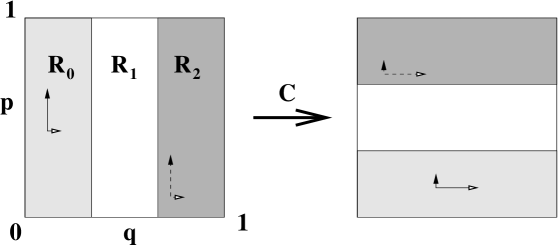
Figure 1: Open baker’s map $C$. The points in the middle rectangle are sent to infinity.

This map is canonical on $S$, and its inverse $C^{-1}$ is defined on the set $C(S)$. Our choice for $S$ coincides with the points $x=(q,p)$ satisfying $\epsilon_{0}(x)\in\{0,2\}$ (equivalently, points s.t. $\epsilon_{0}(x)=1$ are sent to infinity through $C$). This allows us to characterize the trapped sets very easily:

• the forward trapped set $\Gamma_{-}$ (see fig. 2) is made of the points $x$ which will never fall in the strip $R_{1}$ for times $t\geq 0$: these are the points s.t. $\epsilon_{i}\in\{0,2\}$ for all $i\geq 0$, with no constraint on the $\epsilon_{i}$ for $i<0$. This set is of the form $\Gamma_{-}=Can\times[0,1)$, where $Can$ is the standard $1/3$-Cantor set on the unit interval. As a result, the intersection $\Gamma_{-}\cap W_{+}\equiv Can$ has the Hausdorff (or Minkowski) dimension $d=\frac{\log 2}{\log 3}$.

• the backward trapped set $\Gamma_{+}$ is made of the points satisfying $\epsilon_{i}\in\{0,2\}$ for all $i<0$, and is given by $[0,1)\times Can$.

• the full trapped set $K=Can\times Can$.

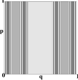
Figure 2: Iterative construction of the forward trapped set $\Gamma_{-}$ for the open baker’s map $C$: we remove from ${\mathbb{T}}^{2}$ the points leaving to infinity at times $t=1,\,2,\,3,\,4$ (from light grey to dark grey) etc. At the end, there remains the fractal set $\Gamma_{-}=Can\times[0,1)$.

2.3 Quantum baker’s map

We now describe in some detail the quantization of the above maps. We recall DEGra ; DBgiens that a nontrivial quantum Hilbert space can be associated with the phase space ${\mathbb{T}}^{2}$ only for discrete values of Planck’s constant, namely $\hbar=(2\pi N)^{-1}$, $N\in{\mathbb{N}}_{0}$. In that case (the only one we will consider), this space ${\mathcal{H}}_{N}$ is of dimension $N$. It admits the “position” basis $\{Q_{j},\ j=0,\ldots,N-1\}$ made of the “Dirac combs”

$$Q_{j}(q)=\frac{1}{\sqrt{N}}\sum_{\nu\in{\mathbb{Z}}}\delta(q-\frac{j}{N}-\nu)\,.$$

This basis is connected to the “momentum” basis $\{P_{k},\,k=0,\ldots,N-1\}$ through the discrete Fourier transform:

$$\langle P_{k}|Q_{j}\rangle=({\mathcal{F}}_{N})_{kj}=\frac{\mathrm{e}^{-2{\rm i}\pi Nkj}}{\sqrt{N}}\,,\quad j,k\in\{0,\ldots,N-1\}\,,$$ (6)

where the Fourier matrix $F_{N}$ is unitary. Balazs and Voros BaVo proposed to quantize the closed baker’s map $B$ as follows, when $N$ is a multiple of $3$ (a condition we will always assume): in the position basis, it takes the block form

$$B_{N}={\mathcal{F}}_{N}^{-1}\left(\begin{array}[]{ccc}{\mathcal{F}}_{N/3}&&\\ &{\mathcal{F}}_{N/3}&\\ &&{\mathcal{F}}_{N/3}\end{array}\right)\,.$$ (7)

This matrix is obviously unitary, and exactly satisfies the Van Vleck formula (the semiclassical expression for a quantum propagator, in terms of the classical generating function). In the semiclassical limit $N\to\infty$, it was shown DENW that these matrices classically propagate Gaussian coherent states supported far enough from the lines of discontinuities. As usual, discontinuities of the classical dynamics induce diffraction effects at the quantum level, which have been partially analyzed for the baker’s map ToVaSa (in particular, diffractive orbits have to be taken into account in the Gutzwiller formula for $\mathrm{tr}(B_{N}^{t})$). We believe that these diffractive effects should only induce lower-order corrections to the Weyl law (9).

We are now ready to quantize our open baker’s map $C$ of (5): since the classical map sends points in $R_{1}$ to infinity and acts through $B$ on $S=R_{0}\cup R_{2}$, the quantum propagator should kill states microsupported on $R_{1}$, and act as $B_{N}$ on states microsupported on $S$. Therefore, in the position basis we get the subunitary matrix

$$C_{N}={\mathcal{F}}_{N}^{-1}\left(\begin{array}[]{ccc}{\mathcal{F}}_{N/3}&&\\ &0&\\ &&{\mathcal{F}}_{N/3}\end{array}\right)\,.$$ (8)

A very similar open quantum baker was constructed in SaVa , as a quantization of Smale’s horseshoe. In Figure 3 (left) we represent the moduli of the matrix elements $(C_{N})_{nm}$. The largest elements are situated along the “tilted diagonals” $n=3m$, $n=3(m-2N/3)$, which correspond to the projection on the $q$-axis of the graph of $C$. Away from these “diagonals”, the amplitudes of the elements decrease relatively slowly (namely, like $1/|n-3m|$). This slow decrease is due to the diffraction effects associated with the discontinuities of the map.

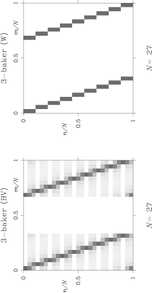
Figure 3: Graphical representation of the matrices $C_{N}$ (8) and $\widetilde{C}_{N}$ (10). Each grey square represents the modulus of a matrix element (white=$0$, black=$1/\sqrt{3}$)

2.4 Resonances of the open baker’s map

We numerically diagonalized the matrices $C_{N}$, for larger and larger Planck’s constants $N$. First of all, we notice that the subspace $\mathrm{Span}\{Q_{j}\,,\ j=N/3,\ldots,2N/3-1\}$, made of position states in the “hole”, is in the kernel of $C_{N}$. Therefore, it is sufficient to diagonalize the matrix obtained by removing the corresponding lines and columns. Upon a slight modification of the quantization procedure Sa , one obtains for $C_{N}$ a matrix covariant w.r.to parity, allowing for a separation of the even and odd eigenstates, and therefore reducing the dimension of each part by $2$. This is the quantization we used for our numerics: we only plot the even-parity resonances (the distribution of the odd-dimensional ones is very similar).

Figure 4: Even-parity spectrum of the matrices $C_{N}$ for $N/3=81,\,2187$

In figure 4 we show the even-parity spectra of the matrix $C_{N}$ for $N=3^{5}$ and $N=3^{8}$. Although we could not detect exact null states for the reduced matrix, many among the $N/3$ eigenvalues had very small moduli: for large values of $N$, the spectrum of $C_{N}$ accumulates near the origin. This accumulation is an obvious consequence of the fractal Weyl law we want to test:

Conjecture 2

For any radius $1>r>0$ and $N\in{\mathbb{N}}_{0}$, $3|N$, let us denote

$$n(N,r)\stackrel{{\scriptstyle\rm{def}}}{{=}}\#\big{\{}\lambda\in\mathrm{Spec}(C_{N})\cap\left\{\,|\lambda|\geq r\,\right\}\big{\}}\,.$$

In the semiclassical limit, this counting function behaves as

$$\frac{n(N,r)}{N^{\frac{\log 2}{\log 3}}}\stackrel{{\scriptstyle N\to\infty}}{{\longrightarrow}}c(r)\,,$$ (9)

with a “shape function” $0\leq c(r)<\infty$.

To test this conjecture, we proceed in two ways:

$\bullet$ In a first step, we select some discrete values for $r$, and plot $n(N,r)$ for an arbitrary sequence of $N$, in a log-log plot (see Fig. 5).

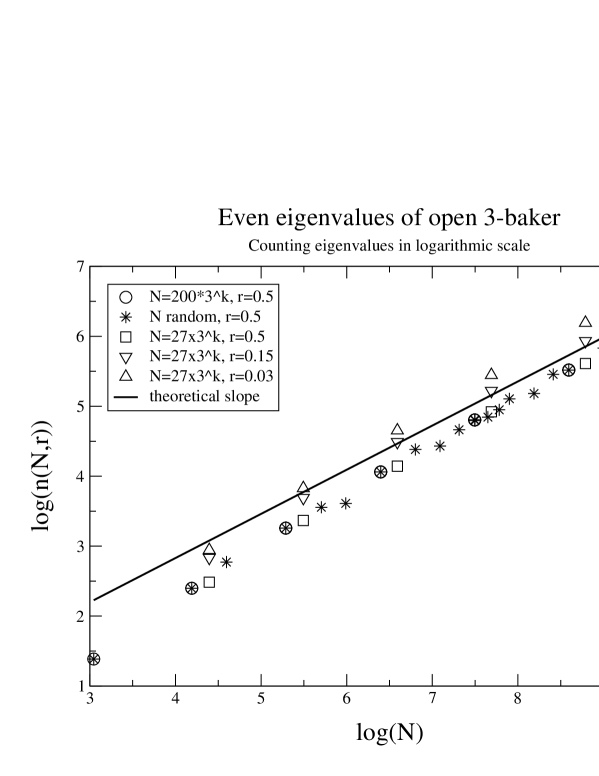
Figure 5: Checking the $N$-dependence of $n(N,r)$ for various values of $r$, along geometric and arbitrary sequences for $N$. The thick curve has the slope $\log 2/\log 3$

We observe that the slope of the data nicely converges towards the theoretical one $\frac{\log 2}{\log 3}$ (thick line), all the more so along geometric subsequences $N=3^{k}\,N_{o}$, and for relatively large values of the radius ($r=0.5$). For the smaller value $r=0.03$, the annulus $\{|z|\geq r\}$ still contains “too many resonances” and the asymptotic régime is not yet reached.

$\bullet$ In a second step, confident that $n(N,r)$ scales like $N^{\frac{\log 2}{\log 3}}$, we try to extract the shape function $c(r)$. For an arbitrary sequence of values of $N$, we plot the function $n(N,r)$ (Fig. 6, left), and then rescale the vertical coordinate by a factor $N^{-\frac{\log 2}{\log 3}}$ (right). The rescaled curves do roughly superpose on one another, supporting the conjecture. However, there remains relatively large fluctuations, even for large values of $N$. The curves corresponding to a geometric sequence $N=3^{k}\,N_{o}$, $k=0,1,\ldots$ tend to be nicely superposed to one another, but slightly differ from one sequence to another. Similar plots were given in schomerus in the case of the kicked rotator; the shape function $c(r)$ is conjectured there to correspond to some ensemble of random subunitary matrices. Our data are too unprecise to perform such a check.

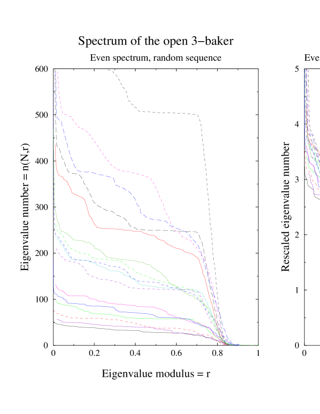
Figure 6: On the left, we plot the number $n(N,r)$ of even eigenvalues of $C_{N}$ of modulus $\geq r$. On the right plot, we rescale those functions by the factors $N^{-\frac{\log 2}{\log 3}}$

The fact that the spectra of the matrices $C_{N}$ “behave nicely” along geometric sequences, while they fluctuate more strongly between successive values of $N$, is not totally unexpected (similar phenomena had been noticed for the quantizations $B_{N}$ of the closed baker BaVo ). In view of Fig. 6, our conjecture (9) may be too strict if we apply it to a general sequence of $N$. At least, it seems to be satisfied along geometric sequences $\left\{\,3^{k}\,N_{o},\,k\in{\mathbb{N}}\,\right\}$, with shape functions $c_{N_{o}}(r)$ slightly depending on the sequence.

3 A solvable toy model for the quantum baker

3.1 Description of the toy model

In an attempt to get some analytical grip on the resonances, we tried to simplify the quantum matrix $C_{N}$, keeping only its “backbone” along the tilted diagonals and removing the off-diagonal components. We obtained the “toy-of-the-toy model” given by the following matrices (the moduli of the components are shown on right plot of Fig. 3):

$$\widetilde{C}_{N=9}=\frac{1}{\sqrt{3}}\left(\begin{array}[]{lllllllll}1&0&0&0&0&0&1&0&0\\ 1&0&0&0&0&0&\omega^{2}&0&0\\ 1&0&0&0&0&0&\omega&0&0\\ 0&1&0&0&0&0&0&1&0\\ 0&1&0&0&0&0&0&\omega^{2}&0\\ 0&1&0&0&0&0&0&\omega&0\\ 0&0&1&0&0&0&0&0&1\\ 0&0&1&0&0&0&0&0&\omega^{2}\\ 0&0&1&0&0&0&0&0&\omega\end{array}\right),\quad\omega=\mathrm{e}^{2\pi{\rm i}/3}\,.$$ (10)

From this example, it is pretty clear how one constructs $\widetilde{C}_{N}$ for $N$ an arbitrary multiple of $3$. A similar quantization of the closed $2$-baker was introduced in schack .

Before describing the spectra of these matrices, we describe their propagation properties. Removing the “off-diagonal” elements, we have eliminated the effects of diffraction due to the discontinuities of $C$. However, this elimination is so abrupt that it modifies the semiclassical transport. Indeed, a coherent state situated at a point $x$ away from the discontinuities will not be transformed by $\widetilde{C}_{N}$ into a single coherent state (as does $C_{N}$), but rather into a linear combination of $3$ coherent states, shifted vertically by $1/3$ from one another. Therefore, the matrices $\widetilde{C}_{N}$ do not quantize the open baker $C$ of (5), but rather the following multivalued (“ray-splitting”) map:

$$\widetilde{C}(q,p)=\left\{\begin{array}[]{ll}(3q,\frac{p}{3})\cup(3q,\frac{p+1}{3})\cup(3q,\frac{p+2}{3})&{\rm if}\ q\in R_{0},\\ (3q-2,\frac{p}{3})\cup(3q-2,\frac{p+1}{3})\cup(3q-2,\frac{p+2}{3})&{\rm if}\ q\in R_{2}.\end{array}\right.$$ (11)

This modification of the classical dynamics is rather annoying. Still, the dynamics $\widetilde{C}$ shares some common features with that of $C$: the forward trapped set for $\widetilde{C}$ is the same as for $C$, that is the set $\Gamma_{-}$ described in Fig. 2. On the other hand, the backward trapped set is now the full torus ${\mathbb{T}}^{2}$.

3.2 Interpretation of $\widetilde{C}_{N}$ as a Walsh-quantized baker

A possible way to avoid this modified classical dynamics is to interpret $\widetilde{C}_{N}$ as a “Walsh-quantized map” (this interpretation makes sense when $N=3^{k}$, $k\in{\mathbb{N}}$). To introduce this Walsh formalism, let us first write the Hilbert space as a tensor product ${\mathcal{H}}_{N}=({\mathbb{C}}^{3})^{\otimes k}$, where we take the ternary decomposition of discrete positions $\frac{j}{N}=0\cdot\epsilon_{0}\epsilon_{1}\cdots\epsilon_{k-1}$ into account. If we call $\{e_{0},\ e_{1},\ e_{2}\}$ the canonical basis of ${\mathbb{C}}^{3}$, each position state $Q_{j}\in{\mathcal{H}}_{N}$ can be represented as the tensor product state

$$Q_{j}=e_{\epsilon_{0}}\otimes e_{\epsilon_{1}}\otimes\cdots\otimes e_{\epsilon_{k-1}}\,.$$

In the language of quantum computing, each tensor factor ${\mathbb{C}}^{3}$ is the Hilbert space of a “qutrit” associated with a certain scale schack .

The Walsh Fourier transform is a modification of the discrete Fourier transform (6), which first appeared in signal theory, and has been recently used as a toy model for harmonic analysis muscalu . Its major advantage is the possibility to construct states compactly supported in both position and “Walsh momentum”. In our finite-dimensional framework, this Walsh transform is the matrix

$$(W_{N})_{jj^{\prime}}=3^{-k/2}\,\exp\Big{(}-\frac{2i\pi}{3}\sum_{\ell+\ell^{\prime}=k-1}\epsilon_{\ell}(Q_{j})\,\epsilon_{\ell^{\prime}}(Q_{j}^{\prime})\Big{)}\,,\qquad j,j^{\prime}=0,\ldots,N-1\,,$$

and acts as follows on tensor product states:

$$W_{N}\,(v_{0}\otimes v_{1}\otimes\cdots v_{k-1})={\mathcal{F}}_{3}v_{k-1}\otimes\cdots{\mathcal{F}}_{3}v_{1}\otimes{\mathcal{F}}_{3}v_{0}\,,\quad v_{\ell}\in{\mathbb{C}}^{3},\ \ell=0,\ldots,k-1\,.$$

Now, in the case $N=3^{k}$, our toy model $\widetilde{C}_{N}$ can be expressed as

$$\widetilde{C}_{N}=W_{N}^{-1}\left(\begin{array}[]{ccc}W_{N/3}&&\\ &0&\\ &&W_{N/3}\end{array}\right)\,.$$

One can show that “Walsh coherent states” are propagated through $\widetilde{C}_{N}$ according to the map $C$. Hence, as opposed to what happens in “standard” quantum mechanics, $\widetilde{C}_{N}$ Walsh-quantizes the open baker $C$.

3.3 Resonances of $\widetilde{C}_{N=3^{k}}$

We now use the very peculiar properties of the matrices $\widetilde{C}_{3^{k}}$ to analytically compute their spectra.

Figure 7: Spectra of the matrices $\widetilde{C}_{N}$ for $N=3^{10}$ (circles), $N=3^{15}$ (crosses). The large circles have radii $|\lambda|=1,\,|\lambda_{+}|,\,|\lambda_{+}\lambda_{-}|^{\frac{1}{2}},\,|\lambda_{-}|$

From the expressions in last section, one can see that the toy model $\widetilde{C}_{N}$ acts very simply on tensor product states:

$$\widetilde{C}_{N}\,v_{0}\otimes v_{1}\otimes\cdots v_{k-1}=v_{1}\otimes\cdots v_{k-1}\otimes{\mathcal{F}}^{-1}_{3}\pi_{02}v_{0}\,,$$ (12)

where $\pi_{02}$ projects ${\mathbb{C}}^{3}$ orthogonally onto $\mathrm{Span}\left\{\,e_{0},\,e_{2}\,\right\}$. Like its classical counterpart, $\widetilde{C}_{N}$ realizes a symbolic shift between the different scales. It also sends the first symbol $\epsilon_{0}$ to the “end of the queue”, after a projection and a Fourier transform. The projection $\pi_{02}$ kills the states $Q_{j}$ localized in the rectangle $R_{1}$. The vector ${\mathcal{F}}^{-1}_{3}e_{\epsilon_{0}}$ in the last qutrit induces a localization in the momentum direction, near the momentum $p=0\cdot\epsilon_{0}$.

By iterating this expression $k$ times, we see that the operator $(\widetilde{C}_{N})^{k}$ acts independently on each tensor factor ${\mathbb{C}}^{3}$, through the matrix ${\mathcal{F}}^{-1}_{3}\pi_{02}$. The latter has three eigenvalues:

• it kills the state $e_{1}$, implying that $(\widetilde{C}_{N})^{k}$ kills any state $Q_{j}$ for which at least one of the symbols $\epsilon_{\ell}(Q_{j})$ is equal to $1$. These $3^{k}-2^{k}$ position states are localized “outside” of the trapped set $\Gamma_{-}$, which explains why they are killed by the dynamics.

• its two remaining eigenvalues $\lambda_{\pm}$ have moduli $|\lambda_{+}|\approx 0.8443$, $|\lambda_{-}|\approx 0.6838$. They build up the ($2^{k}$-dimensional) nontrivial spectrum of $\widetilde{C}_{N}$, which has the form of a “lattice” (see Fig. 7):

Proposition 1

For $N=3^{k}$, the nonzero spectrum of $\widetilde{C}_{N}$ is the set

$$\left\{\,\lambda_{+}\,\right\}\cup\left\{\,\lambda_{-}\,\right\}\bigcup\left\{\,\mathrm{e}^{2{\rm i}\pi\frac{j}{k}}\,\lambda_{+}^{1-p/k}\lambda_{-}^{p/k}\;:\;1\leq p\leq k-1\,,\ 0\leq j\leq k-1\,\right\}\,.$$

Most of these eigenvalues are highly degenerate (they span a subspace of dimension $2^{k}$). When $k\to\infty$, the highest degeneracies occur when $p/k\approx 2$, which results in the following asymptotic distribution:

$$\forall f\in C({\mathbb{R}}^{2}),\quad\lim_{k\to\infty}\ \frac{1}{2^{k}}\sum_{\lambda\in\mathrm{Spec}(\widetilde{C}_{3^{k}})\setminus 0}\mathrm{mult}(\lambda)\,f(\lambda)=\int_{0}^{2\pi}f(|\lambda_{-}\lambda_{+}|^{1/2},\theta)\,\frac{\mathrm{d}\theta}{2\pi}\,.$$

The last formula shows that the spectrum of $\widetilde{C}_{N}$ along the geometric sequence $\{N=3^{k},\,k\in{\mathbb{N}}\}$ satisfies the fractal Weyl law (9), with a shape function in form of an abrupt step: $c(r)=\Theta(|\lambda_{+}\lambda_{-}|^{1/2}-r)$. Although the above spectrum seems very nongeneric (lattice structure, singular shape function), it is the first example (to our knowledge) of a quantum open system proven to satisfy the fractal Weyl law.

Acknowledgments. We benefited from insightful discussions with Marcos Saraceno, André Voros, Uzy Smilansky, Christof Thiele and Terry Tao. Part of the work was done while I was visiting M. Zworski in UC Berkeley, supported by the grant DMS-0200732 of the National Science Foundation.

References

- (1) N.L. Balazs and A. Voros The quantized baker’s transformation, Ann. Phys. 190 (1989), 1–31.
- (2) R. Blümel and U. Smilansky, A simple model for chaotic scattering, Physica D 36 (1989), 111–136.
- (3) N. Chernov and R. Markarian, Ergodic properties of Anosov maps with rectangular holes, Boletim Sociedade Brasileira Matematica 28 (1997), 271–314.
- (4) N. Chernov, R. Markarian and S. Troubetzkoy, Conditionally invariant measures for Anosov maps with small holes, Ergod. Th. Dyn. Sys. 18 (1998), 1049–1073.
- (5) P. Cvitanović and B. Eckhardt, Periodic-orbit quantization of chaotic systems, Phys. Rev. Lett. 63 (1989) 823–826
- (6) S. De Bièvre, Recent results on quantum map eigenstates, these Proceedings.
- (7) M. Degli Esposti and S. Graffi, editors The mathematical aspects of quantum maps, volume 618 of Lecture Notes in Physics, Springer, 2003.
- (8) M. Degli Esposti, S. Nonnenmacher and B. Winn, Quantum variance and ergodicity for the baker’s map, to be published in Commun. Math. Phys. (2005), arXiv:math-ph/0412058.
- (9) P. Gaspard and S.A. Rice, Scattering from a classically chaotic repellor, J. Chem. Phys. 90 (1989), 2225–2241; ibid, Semiclassical quantization of the scattering from a classically chaotic repellor, J. Chem. Phys. 90 (1989), 2242–54; ibid, Exact quantization of the scattering from a classically chaotic repellor, J. Chem. Phys. 90 (1989), 2255–2262; Errata, J. Chem. Phys. 91 (1989), 3279–3280.
- (10) L. Guillopé, K. Lin, and M. Zworski, The Selberg zeta function for convex co-compact Schottky groups, Comm. Math. Phys, 245(2004), 149–176.
- (11) V. Ivrii, Microlocal Analysis and Precise Spectral Asymptotics, Springer Verlag, 1998.
- (12) K. Lin, Numerical study of quantum resonances in chaotic scattering, J. Comp. Phys. 176(2002), 295–329.
- (13) K. Lin and M. Zworski, Quantum resonances in chaotic scattering, Chem. Phys. Lett. 355(2002), 201–205.
- (14) W. Lu, S. Sridhar, and M. Zworski, Fractal Weyl laws for chaotic open systems, Phys. Rev. Lett. 91(2003), 154101.
- (15) C. Muscalu, C. Thiele, and T. Tao, A Carleson-type theorem for a Cantor group model of the Scattering Transform, Nonlinearity 16 (2003), 219–246.
- (16) S. Nonnenmacher and M. Zworski, Distribution of resonances for open quantum maps, preprint, 2005.
- (17) M. Saraceno, Classical structures in the quantized baker transformation, Ann. Phys. (NY) 199 (1990), 37–60.
- (18) M. Saraceno and R.O. Vallejos, The quantized D-transformation, Chaos 6 (1996), 193–199.
- (19) R. Schack and C.M. Caves, Shifts on a finite qubit string: a class of quantum baker’s maps, Appl. Algebra Engrg. Comm. Comput. 10 (2000) 305–310
- (20) H. Schomerus and J. Tworzydło, Quantum-to-classical crossover of quasi-bound states in open quantum systems, Phys. Rev. Lett. 93 (2004), 154102.
- (21) J. Sjöstrand, Geometric bounds on the density of resonances for semiclassical problems, Duke Math. J., 60 (1990), 1–57.
- (22) J. Sjöstrand, Semiclassical resonances generated by a non-degenerate critical point, Lecture Notes in Math. 1256, 402–429, Springer (Berlin), 1987.
- (23) J. Sjöstrand and M. Zworski, Lower bounds on the number of scattering poles, Commun. PDE 18 (1993), 847–857.
- (24) J. Sjöstrand and M. Zworski, Geometric bounds on the density of semiclassical resonances in small domains, in preparation (2005).
- (25) F. Toscano, R.O. Vallejos and M. Saraceno, Boundary conditions to the semiclassical traces of the baker’s map, Nonlinearity 10 (1997), 965–978.
- (26) G. Troll and U. Smilansky, A simple model for chaotic scattering, Physica D 35 (1989), 34–64.
- (27) M. Zworski, Dimension of the limit set and the density of resonances for convex co-compact Riemann surfaces, Inv. Math. 136 (1999), 353–409.