VARIATIONAL PROBLEMS IN ELASTIC THEORY OF BIOMEMBRANES, SMECTIC-A LIQUID CRYSTALS, AND CARBON RELATED STRUCTURES

Abstract

After a brief introduction to several variational problems in the study of shapes of thin structures, we deal with variational problems on 2-dimensional surface in 3-dimensional Euclidian space by using exterior differential forms and the moving frame method. The morphological problems of lipid bilayers and stabilities of cell membranes are also discussed. The key point is that the first and the second order variations of the free energy determine equilibrium shapes and mechanical stabilities of structures.

1 Introduction

The morphology of thin structures (always represented by a smooth surface $M$ in this paper) is an old problem. First, we look back on the history [21]. As early as in 1803, Plateau studied a soap film attaching to a metallic ring when the ring passed through soap water [25]. By taking the minimum of the free energy $F=\lambda\int_{M}\mathrm{d}A$, he obtained $H=0$, where $\lambda$ and $H$ are the surface tension and mean curvature of the soap film, respectively. From 1805 and 1806, Young [37] and Laplace [11] studied soap bubbles. By taking the minimum of the free energy $F=p\int\mathrm{d}V+\lambda\oint_{M}\mathrm{d}A$, they obtained $H=p/2\lambda$, where $p$ is the osmotic pressure (pressure difference between outer and inner sides) of a soap bubble and $V$ is the volume enclosed by the bubble. We can only observe spherical bubbles because “An embedded surface with constant mean curvature in 3-dimensional (3D) Euclidian space ($\mathbb{E}^{3}$) must be a spherical surface” [1]. In 1812, Poisson [26] considered a solid shell and put forward the free energy $F=\oint_{M}H^{2}\mathrm{d}A$. Its Euler-Lagrange equation is $\nabla^{2}H+2H(H^{2}-K)=0$ [36]. Now the solutions to this equation are called Willmore surfaces. In 1973, Helfrich recognized that lipid bilayers could be regarded as smectic-A (SmA) liquid crystals (LCs) at room temperature. Based on the elastic theory of liquid crystals [4], he proposed the curvature energy per unit area of the bilayer

$$\mathcal{E}_{lb}=(k_{c}/2)(2H+c_{0})^{2}+\bar{k}K,$$ (1)

where $k_{c}$ and $\bar{k}$ are elastic constants. $K$ and $c_{0}$ are Gaussian curvature and spontaneous curvature of the lipid bilayer, respectively. Starting with Helfrich’s curvature energy (1), the morphology of lipid vesicles has been deeply understood [15, 24, 28]. Especially, the free energy is expressed as $F=p\int\mathrm{d}V+\oint_{M}(\lambda+\mathcal{E}_{lb})\mathrm{d}A$ for lipid vesicles, and the corresponding Euler-Lagrange equation is [22]:

$$p-2\lambda H+k_{c}\nabla^{2}(2H)+k_{c}(2H+c_{0})(2H^{2}-c_{0}H-2K)=0.$$ (2)

For an open lipid bilayer with a free edge $C$, the free energy is expressed as $F=\int_{M}(\lambda+\mathcal{E}_{lb})\mathrm{d}A+\gamma\oint_{C}\mathrm{d}s$, where $\gamma$ is the line tension of the edge. The corresponding Euler-Lagrange equations are as follows [3, 31]:

$$k_{c}(2H+c_{0})(2H^{2}-c_{0}H-2K)-2\lambda H+k_{c}\nabla^{2}(2H) =0$$ (3)

$$\left.\left[k_{c}(2H+c_{0})+\bar{k}k_{n}\right]\right|_{C} =0$$ (4)

$$\left.\left[-2k_{c}\frac{\partial H}{\partial\mathbf{e}_{2}}+\gamma k_{n}+\bar{k}\frac{d\tau_{g}}{ds}\right]\right|_{C} =0$$ (5)

$$\left.\left[\frac{k_{c}}{2}(2H+c_{0})^{2}+\bar{k}K+\lambda+\gamma k_{g}\right]\right|_{C} =0,$$ (6)

where $k_{n}$, $k_{g}$, and $\tau_{g}$ are normal curvature, geodesic curvature, and geodesic torsion of the boundary curve. The unit vector $\mathbf{e}_{2}$ (see also Fig. 1) is perpendicular to tangent vector of edge $C$ and normal vector of surface $M$. Above four equations are called the shape equation and boundary conditions of open lipid bilayers. The boundary conditions are available for open lipid bilayers with more than one edge because the edge in our derivation [31] is a general one.

Secondly, we turn to the puzzle about the formation of focal conic structures in SmA LCs. As we imagine, the configuration of minimum energy in SmA LCs is a flat layer structure. But Dupin cyclides are usually formed when LCs cool from isotropic phase to SmA phase in the experiment [7]. Why the cyclides are preferred to other geometrical structures under the preservation of the interlayer spacing [2]? This phenomenon can be understood by the concept that the Gibbs free energy difference between isotropic and SmA phases must be balanced by the curvature elastic energy of SmA layers [17]. The total free energy includes curvature energy, volume energy and surface energy. It is expressed formally as $F=\oint\mathcal{E}(H,K,t)\mathrm{d}A$, where $t$ is the thickness of the focal conic domain; $H$ and $K$ are mean curvature and Gaussian curvature of the inmost layer surface, respectively. The Euler-Lagrange equations corresponding to the free energy are as follows [19]:

$$\oint(\partial\mathcal{E}/\partial t)\mathrm{d}A =0$$ (7)

$$(\nabla^{2}/2+2H^{2}-K)\partial\mathcal{E}/\partial H+(\nabla\cdot\tilde{\nabla}+2KH)\partial\mathcal{E}/\partial K-2H\mathcal{E} =0.$$ (8)

Solving both equations can give good explanation to focal conic domains [19]. The new operator $\tilde{\nabla}$ can be found in in the appendix of Ref. [32].

Thirdly, let us see carbon related structures. There are three typical structures composed of carbon atoms: Buckyball (C₆₀), single-walled carbon nanotube (SWNT), and carbon torus. In the continuum limit, we derive the curvature energy [23, 30] of single graphitic layer $E=\int\left[\frac{1}{2}k_{c}(2H)^{2}+\bar{k}K\right]\mathrm{d}A$ from the lattice model [13], where $k_{c}$ and $\bar{k}$ are elastic constants. The total free energy of a graphite layer is $F=\int\left[\frac{1}{2}k_{c}(2H)^{2}+\bar{k}K\right]\mathrm{d}A+\lambda\int\mathrm{d}A$, where $\lambda$ is the surface energy per unit area for graphite. Please note that the surface energy per unit area for solid structures is not as a constant quantity as the surface tension for fluid membranes. The Euler-Lagrange equation corresponding to the free energy is $\nabla^{2}H+2H(H^{2}-K)-\lambda H/k_{c}=0$. C₆₀ and carbon torus can be understood with $\lambda=0$, while SWNT satisfies $R^{2}=k_{c}/2\lambda$, where $R$ is its radius.

The rest of this paper is organized as follows. In Sec. 2, we show how to derive the Euler-Lagrange equation from the free energy functional by using exterior differential forms. The method is developed in Refs. [31] and [32], which might be equivalent to the work by Griffiths [9] in essence. But it is more convenient to apply in variational problems on 2D surface in $\mathbb{E}^{3}$. In Sec. 3, we give several analytic solutions to the shape equation of lipid vesicles, and to the shape equation and boundary conditions of open lipid bilayers. In Sec. 4, we discuss the elasticity and stability of cell membranes. A brief summary is given in the last section.

2 Variational problems on 2D surface

Many variational problems are shown in Introduction. Here we deal with them by using exterior differential forms.

Let us consider a surface $M$ with an edge $C$ as shown in Fig. 1. At every point P in the surface, we can choose a right-handed, orthonormal frame {$\mathbf{e}_{1},\mathbf{e}_{2},\mathbf{e}_{3}$} with $\mathbf{e}_{3}$ being the normal vector. For a point in curve $C$, $\mathbf{e}_{1}$ is the tangent vector of $C$ such that $\mathbf{e}_{2}$ points to the side that the surface is located in.

The differential of the frame is expressed as

$$\mathrm{d}\mathbf{r} =\omega_{1}\mathbf{e}_{1}+\omega_{2}\mathbf{e}_{2}$$ (9)

$$\mathrm{d}\mathbf{e}_{i} =\omega_{ij}\mathbf{e}_{j},\quad(i=1,2,3)$$ (10)

where $\omega_{1}$, $\omega_{2}$, $\omega_{ij}=-\omega_{ji}$ ($i,j=1,2,3$) are 1-forms. Please note that the repeated subindex represents the summation from 1 to 3, unless otherwise specified in this paper.

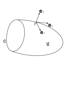
Figure 1: A surface $M$ with an edge $C$. {$\mathbf{e}_{1},\mathbf{e}_{2},\mathbf{e}_{3}$} is an orthonormal frame.

The structure equations of the surface are as follows:

$$\mathrm{d}\omega_{1} =\omega_{12}\wedge\omega_{2}$$ (11)

$$\mathrm{d}\omega_{2} =\omega_{21}\wedge\omega_{1}$$ (12)

$$\omega_{13} =a\omega_{1}+b\omega_{2},\omega_{23}=b\omega_{1}+c\omega_{2}$$ (13)

$$\mathrm{d}\omega_{ij} =\omega_{ik}\wedge\omega_{kj}\quad(i,j=1,2,3),$$ (14)

where $a$, $b$, $c$ are related to the curvatures with $2H=a+c$ and $K=ac-b^{2}$.

The variation of the frame is denoted by

$$\delta\mathbf{r} =\delta_{1}\mathbf{r}+\delta_{2}\mathbf{r}+\delta_{3}\mathbf{r}$$ (15)

$$\delta_{i}\mathbf{r} =\Omega_{i}\mathbf{e}_{i}\quad(i=1,2,3)$$ (16)

$$\delta_{l}\mathbf{e}_{i} =\Omega_{lij}\mathbf{e}_{j},(i,l=1,2,3),$$ (17)

with $\Omega_{lij}=-\Omega_{lji}$ ($i,j,l=1,2,3$). In equation (16), the repeated subindex does not represent summation. It is easy to prove that the operator $\delta_{l}(l=1,2,3)$ has the similar properties with the partial differential while the operator $\delta$ has the similar properties with the total differential operator [32].

Using $\mathrm{d}\delta_{l}\mathbf{r}=\delta_{l}\mathrm{d}\mathbf{r}$ and $\mathrm{d}\delta_{l}\mathbf{e}_{i}=\delta_{l}\mathrm{d}\mathbf{e}_{i}$, we obtain variational equations of the frame as follows [32]:

$$\delta_{1}\omega_{1} =\mathrm{d}\Omega_{1}-\omega_{2}\Omega_{121}$$ (18)

$$\delta_{1}\omega_{2} =\Omega_{1}\omega_{12}-\omega_{1}\Omega_{112}$$ (19)

$$\Omega_{113} =a\Omega_{1},\quad\Omega_{123}=b\Omega_{1};$$ (20)

$$\delta_{2}\omega_{1} =\Omega_{2}\omega_{21}-\omega_{2}\Omega_{221}$$ (21)

$$\delta_{2}\omega_{2} =\mathrm{d}\Omega_{2}-\omega_{1}\Omega_{212}$$ (22)

$$\Omega_{213} =b\Omega_{2},\quad\Omega_{223}=c\Omega_{2};$$ (23)

$$\delta_{3}\omega_{1}=\Omega_{3}\omega_{31}-\omega_{2}\Omega_{321}$$ (24)

$$\delta_{3}\omega_{2}=\Omega_{3}\omega_{32}-\omega_{1}\Omega_{312}$$ (25)

$$\mathrm{d}\Omega_{3}=\Omega_{313}\omega_{1}+\Omega_{323}\omega_{2};$$ (26)

$$\delta_{l}\omega_{ij}=\mathrm{d}\Omega_{lij}+\Omega_{lik}\omega_{kj}-\omega_{ik}\Omega_{lkj}.$$ (27)

Using them, we can prove that

$$\delta_{1}(\mathcal{E}\omega_{1}\wedge\omega_{2}) =\mathrm{d}(\mathcal{E}\omega_{2}\Omega_{1})$$ (28)

$$\delta_{2}(\mathcal{E}\omega_{1}\wedge\omega_{2}) =-\mathrm{d}(\mathcal{E}\omega_{1}\Omega_{2})$$ (29)

$$\delta_{3}(\omega_{1}\wedge\omega_{2}) =-2H\Omega_{3}\omega_{1}\wedge\omega_{2}$$ (30)

$$\delta_{3}(2H)\omega_{1}\wedge\omega_{2} =2(2H^{2}-K)\Omega_{3}\omega_{1}\wedge\omega_{2}+\mathrm{d}\ast\mathrm{d}\Omega_{3}$$ (31)

$$\delta_{3}K\omega_{1}\wedge\omega_{2} =2KH\Omega_{3}\omega_{1}\wedge\omega_{2}+\mathrm{d}\tilde{\ast}\tilde{\mathrm{d}}\Omega_{3},$$ (32)

where $\mathcal{E}$ is a function of $2H$ and $K$. $\ast$ is Hodge star operator [35] satisfying the following properties: (i) $\ast f=f\omega_{1}\wedge\omega_{2}$ for scalar function $f$; (ii) $\ast\omega_{1}=\omega_{2}$, $\ast\omega_{2}=-\omega_{1}$. $\tilde{\ast}$ and $\tilde{\mathrm{d}}$ are new operators defined in Ref. [32] that satisfy: (i) If $df=f_{1}\omega_{1}+f_{2}\omega_{2}$, then $\tilde{\mathrm{d}}f=f_{1}\omega_{13}+f_{2}\omega_{23}$; (ii) $\tilde{\ast}\omega_{13}=\omega_{23},\tilde{\ast}\omega_{23}=-\omega_{13}$; (iii) $\int_{M}(f\mathrm{d}{\ast}\tilde{\mathrm{d}}h-h\mathrm{d}{\ast}\tilde{\mathrm{d}}f)=\int_{\partial M}(f{\ast}\tilde{\mathrm{d}}h-h{\ast}\tilde{\mathrm{d}}f)$, $\int_{M}(f\mathrm{d}\tilde{\ast}\tilde{\mathrm{d}}h-h\mathrm{d}\tilde{\ast}\tilde{\mathrm{d}}f)=\int_{\partial M}(f\tilde{\ast}\tilde{\mathrm{d}}h-h\tilde{\ast}\tilde{\mathrm{d}}f)$ for any smooth functions $f$ and $h$ on $M$.

Now, we consider the variational problem on closed surface. In this case, the general functional is expressed as:

$$F=\oint_{M}\mathcal{E}(2H,K)\mathrm{d}A+p\int_{V}\mathrm{d}V.$$ (33)

Using Stokes theorem and the variational equations of the frame, we can prove that

$$\delta_{1}\int_{V}\mathrm{d}V =\delta_{2}\int_{V}\mathrm{d}V=0$$ (34)

$$\delta_{3}\int_{V}\mathrm{d}V =\oint_{M}\Omega_{3}\mathrm{d}A.$$ (35)

Combining them with equations (28)–(32), we have $\delta_{1}F=\delta_{2}F=0$, and the Euler-Lagrange equation corresponding to functional (33):

$$\left[\left(\nabla^{2}+4H^{2}-2K\right)\frac{\partial}{\partial(2H)}+\left(\nabla\cdot\tilde{\nabla}+2KH\right)\frac{\partial}{\partial K}-2H\right]\mathcal{E}+p=0.$$ (36)

Next, we consider the variational problem on open surface with an edge $C$. In this case, the general functional is expressed as:

$$F=\int_{M}\mathcal{E}(2H,K)\mathrm{d}A+\oint_{C}\Gamma(k_{n},k_{g})\mathrm{d}s.$$ (37)

Similarly, we derive its Euler-Lagrange equations as

$$(\nabla^{2}+4H^{2}-2K)\frac{\partial\mathcal{E}}{\partial(2H)}+(\nabla\cdot\tilde{\nabla}+2KH)\frac{\partial\mathcal{E}}{\partial K}-2H\mathcal{E}=0$$ (38)

$$\mathbf{e}_{2}\cdot\nabla\left[\frac{\partial\mathcal{E}}{\partial(2H)}\right]+\mathbf{e}_{2}\cdot\tilde{\nabla}\left(\frac{\partial\mathcal{E}}{\partial K}\right)-\frac{d}{ds}\left(\tau_{g}\frac{\partial\mathcal{E}}{\partial K}\right)+\frac{d^{2}}{ds^{2}}\left(\frac{\partial\Gamma}{\partial k_{n}}\right)+\frac{\partial\Gamma}{\partial k_{n}}(k_{n}^{2}-\tau_{g}^{2})$$

$$\quad+\tau_{g}\frac{d}{ds}\left(\frac{\partial\Gamma}{\partial k_{g}}\right)+\frac{d}{ds}\left(\tau_{g}\frac{\partial\Gamma}{\partial k_{g}}\right)-\left.\left(\Gamma-\frac{\partial\Gamma}{\partial k_{g}}k_{g}\right)k_{n}\right|_{C}=0$$ (39)

$$-\frac{\partial\mathcal{E}}{\partial(2H)}-k_{n}\frac{\partial\mathcal{E}}{\partial K}+\frac{\partial\Gamma}{\partial k_{g}}k_{n}-\left.\frac{\partial\Gamma}{\partial k_{n}}k_{g}\right|_{C}=0$$ (40)

$$\frac{d^{2}}{ds^{2}}\left(\frac{\partial\Gamma}{\partial k_{g}}\right)+K\frac{\partial\Gamma}{\partial k_{g}}-k_{g}\left(\Gamma-\frac{\partial\Gamma}{\partial k_{g}}k_{g}\right)+2(k_{n}-H)k_{g}\frac{\partial\Gamma}{\partial k_{n}}$$

$$\quad-\tau_{g}\frac{d}{ds}\left(\frac{\partial\Gamma}{\partial k_{n}}\right)\left.-\frac{d}{ds}\left(\tau_{g}\frac{\partial\Gamma}{\partial k_{n}}\right)-\mathcal{E}\right|_{C}=0.$$ (41)

In special cases, above equations (36), (38)–(41) are degenerated into different equations mentioned in Introduction. For example, if taking $\mathcal{E}=\mathcal{E}_{lb}+\lambda$ and $\Gamma=\gamma$, These equations are degenerated into equations (3)–(6), respectively.

3 Morphology of lipid bilayers

There are three typical solutions to shape equation (2): Sphere, torus, and biconcave vesicle.

First, a spherical vesicle with radius $R$ satisfies equation (2) if $pR^{2}+2\lambda R-k_{c}c_{0}(2-c_{0}R)=0$ is valid. Secondly, Ou-Yang used equation (2) to predict that a torus with the radii of two generating circles $r$ and $R$ satisfying $R/r=\sqrt{2}$ should be observed in lipid systems [20]. This striking prediction has been confirmed experimentally by three groups [14, 16, 27]. Thirdly, the first exact axisymmetric solution with biconcave shape, as shown in Fig. 2, was found under the condition of $p=\lambda=0$ as [18]:

$$z =z_{0}+\int_{0}^{\rho}\tan\psi(\rho^{\prime})d\rho^{\prime}$$ (42)

$$\sin\psi(\rho) =-c_{0}\rho\ln(\rho/\rho_{B}),c_{0}>0,$$ (43)

where $z(\rho)$ is the contour of the cross-section. $z$ axis is the rotational axis, and $\psi(\rho)$ the tangent angle of the contour at distance $\rho$. This solution can explain the classic physiological puzzle [8]: Why the red blood cells of humans are always in biconcave shape?

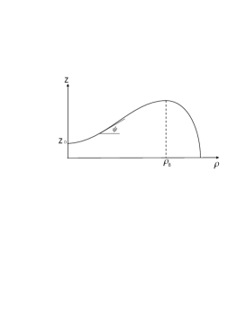
Figure 2: Schematic figure of the contour of biconcave vesicle in the first quadrant.

To the shape equation (3) and boundary conditions (4)–(6) of open lipid bilayers, we can find two analytical solutions [31]: One is the central part of a torus and another is a cup-like membrane shown in Fig. 3. Numerical method and solutions to these equations can be find in Ref. [33].

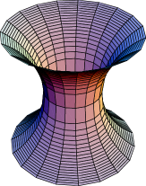
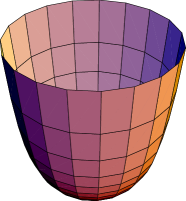
Figure 3: The central part of a torus (left) and a cup-like membrane (right).

4 Elasticity and stability of cell membranes

A cell membrane is simplified as lipid bilayer plus membrane skeleton. The skeleton is a cross-linking protein network and joint to the bilayer at some points. We know that the cross-linking polymer structure also exists in rubber at molecular levels. Thus we can transplant the theory of rubber elasticity [29] to describe the membrane skeleton.

Based on Helfrich’s theory and physics of rubber elasticity, the free energy of a closed cell membrane can be expressed as [32]:

$$F=\oint_{M}(\mathcal{E}_{d}+\mathcal{E}_{H})\mathrm{d}A+p\int_{V}\mathrm{d}V,$$ (44)

with $\mathcal{E}_{H}=(k_{c}/2)(2H+c_{0})^{2}+\lambda$ and $\mathcal{E}_{d}=(k_{d}/2)[(2J)^{2}-Q]$, where $2J=\varepsilon_{11}+\varepsilon_{22}$, $Q=\varepsilon_{11}\varepsilon_{22}-\varepsilon_{12}^{2}$. Here $\varepsilon_{ij}$ ($i,j=1,2$) represents the in-plane strain of the membrane. $k_{d}$ is the elastic constant representing the entropic elasticity [5] of membrane skeleton.

Using the method in Sec. 2, we obtain the shape equation and the in-plane strain equations of the cell membrane as [32]:

$$p-2H(\lambda+k_{d}J)+k_{c}(2H+c_{0})(2H^{2}-c_{0}H-2K)$$

$$\qquad+k_{c}\nabla^{2}(2H)-\frac{k_{d}}{2}(a\varepsilon_{11}+2b\varepsilon_{12}+c\varepsilon_{22})=0$$ (45)

$$k_{d}[-\mathrm{d}(2J)\wedge\omega_{2}-\frac{1}{2}(\varepsilon_{11}\mathrm{d}\omega_{2}-\varepsilon_{12}\mathrm{d}\omega_{1})+\frac{1}{2}\mathrm{d}(\varepsilon_{12}\omega_{1}+\varepsilon_{22}\omega_{2})]=0$$ (46)

$$k_{d}[\mathrm{d}(2J)\wedge\omega_{1}-\frac{1}{2}(\varepsilon_{12}\mathrm{d}\omega_{2}-\varepsilon_{22}\mathrm{d}\omega_{1})-\frac{1}{2}\mathrm{d}(\varepsilon_{11}\omega_{1}+\varepsilon_{12}\omega_{2})]=0.$$ (47)

An obvious solution is the spherical cell membrane with homogenous strains: $\varepsilon_{11}=\varepsilon_{22}=\varepsilon$ (a constant) and $\varepsilon_{12}=0$. The radius $R$ of the sphere must satisfy

$$pR^{2}+(2\lambda+3k_{d}\varepsilon)R+k_{c}c_{0}(c_{0}R-2)=0.$$ (48)

Now we will show the biological function of membrane skeleton by discussing the mechanical stability of a spherical cell membrane. Using Hodge decomposed theorem [35], $\Omega_{1}$ and $\Omega_{2}$ can be expressed as $\Omega_{1}\omega_{1}+\Omega_{2}\omega_{2}=d\Omega+\ast d\chi$ by two scalar functions $\Omega$ and $\chi$. Through complex calculations, we obtain the second order variation of the free energy for spherical membrane $\delta^{2}\mathcal{F}=G_{1}+G_{2}$, where

$$G_{1} =\oint_{M}\Omega_{3}^{2}\{3k_{d}/R^{2}+(2k_{c}c_{0}/R^{3})+p/R\}\mathrm{d}A$$

$$+\oint_{M}\Omega_{3}\nabla^{2}\Omega_{3}\{k_{c}c_{0}/R+2k_{c}/R^{2}+pR/2\}\mathrm{d}A$$

$$+\oint_{M}k_{c}(\nabla^{2}\Omega_{3})^{2}\mathrm{d}A+\frac{3k_{d}}{R}\oint_{M}\Omega_{3}\nabla^{2}\Omega\mathrm{d}A$$

$$+k_{d}\oint_{M}\left(\nabla^{2}\Omega\right)^{2}\mathrm{d}A+\frac{k_{d}}{2R^{2}}\oint_{M}\Omega\nabla^{2}\Omega\mathrm{d}A,$$ (49)

and $G_{2}=(k_{d}/4)\oint_{M}\nabla^{2}\chi(\nabla^{2}\chi+2\chi/R^{2})\mathrm{d}A$. Because $G_{2}$ is positive definite, we merely need to discuss $G_{1}$. $\Omega_{3}$ and $\Omega$ in the expression of $G_{1}$ are arbitrary functions defined in a sphere and can be expanded by spherical harmonic functions [34]: $\Omega_{3}=\sum_{l=0}^{\infty}\sum_{m=-l}^{m=l}a_{lm}Y_{lm}(\theta,\phi)$ and $\Omega=\sum_{l=0}^{\infty}\sum_{m=-l}^{m=l}b_{lm}Y_{lm}(\theta,\phi)$ with $a_{lm}^{*}=(-1)^{m}a_{l,-m}$ and $b_{lm}^{*}=(-1)^{m}b_{l,-m}$. Considering (48), we write $G_{1}$ in a quadratic form:

$$G_{1} =\sum_{l=0}^{\infty}\sum_{m=0}^{l}2|a_{lm}|^{2}\{3k_{d}+[l(l+1)-2][l(l+1){k}_{c}/R^{2}-{k}_{c}{c}_{0}/R-pR/2]\}$$

$$-\sum_{l=0}^{\infty}\sum_{m=0}^{l}\frac{3k_{d}}{R}l(l+1)(a_{lm}^{\ast}b_{lm}+a_{lm}b_{lm}^{\ast})$$

$$+\sum_{l=0}^{\infty}\sum_{m=0}^{l}\frac{k_{d}}{R^{2}}\left[2l^{2}(l+1)^{2}-l(l+1)\right]|b_{lm}|^{2}.$$ (50)

It is easy to prove that, if $p<p_{l}=\frac{3k_{d}}{\left[2l(l+1)-1\right]R}+\frac{2{k}_{c}[l(l+1)-{c}_{0}R]}{R^{3}}\quad(l=2,3,\cdots)$, then $G_{1}$ is positive definite. Thus we must take the minimum of $p_{l}$ to obtain the critical pressure :

$$p_{c}=\min\{p_{l}\}=\left\{\begin{array}[]{c}\frac{3k_{d}}{11R}+\frac{2k_{c}[6-c_{0}R]}{R^{3}}<\frac{k_{c}[23-2c_{0}R]}{R^{3}},\quad(3k_{d}R^{2}<121k_{c})\\ \frac{2\sqrt{3k_{d}k_{c}}}{R^{2}}+\frac{k_{c}}{R^{3}}(1-2c_{0}R),\quad(3k_{d}R^{2}>121k_{c}).\end{array}\right.$$ (53)

Taking typical data of cell membrane, $k_{c}\sim 20k_{B}T$ [6], $k_{d}\sim 6\times 10^{-4}k_{B}T/nm^{2}$ [12], $h\sim 4nm$, $R\sim 1\mu m$, $c_{0}R\sim 1$, we have $p_{c}\sim 2$ Pa from equation (53). If not considering membrane skeleton, that is $k_{d}=0$, we obtain $p_{c}\sim 0.2$ Pa. Therefore, membrane skeleton enhances the mechanical stability of cell membranes, at least for spherical shape.

5 Summary

In above discussion, we introduce several problems in the elasticity of biomembranes, smectic-A liquid crystal, and carbon related structures. We deal with these variational problems on 2D surface by using exterior differential forms. Elasticity and stability of lipid bilayers and cell membranes are calculated and compared with each other. It is shown that membrane skeleton enhances the mechanical stability of cell membranes.

References

- [1] Alexandrov A. D., Uniqueness Theorems for Surfaces in the Large, Amer. Math. Soc. Transl., 21 (1962) 341–416.
- [2] Bragg W., Liquid Crystals Nature 133 (1934) 445.
- [3] Capovilla R., Guven J. and Santiago J.A., Lipid Membranes with an Edge, Phys. Rev. E 66 (2002) 21607.
- [4] de Gennes P. G., The Physics of Liquid Crystals, Clarendon Press, Oxford, 1975.
- [5] de Gennes P. G., Scaling Concepts in Polymer Physics, Cornell University Press, New York, 1979.
- [6] Duwe H P, Kaes J and Sackmann E, Bending Elastic-Moduli of Lipid Bilayers–Modulation by Solutes, J. Phys. Fr. 51 (1990) 945–962.
- [7] Friedel G. and Grandjean F., Observations Geometriques sur les Liquides a Conique Focales, Bull. Soc. fr. Miner. 33 (1910) 409–465.
- [8] Fung Y. C. and Tong P., Theory of the Sphering of Red Blood Cells Biophys. J. 8 (1968) 175–198.
- [9] Griffiths P., Exterior Differential Systems and the Calculus of Variations, Birkhäuser, Boston, 1983.
- [10] Helfrich W., Elastic Properties of Lipid Bilayers–Theory and Possible Experiments, Z. Naturforsch. C 28 (1973) 693.
- [11] Laplace P. S., Traité de Mécanique Céleste, Gauthier-Villars, Paris, 1839.
- [12] Lenormand G., Hénon S., Richert A., Siméon J., and Gallet F., Direct Measurement of the Area Expansion and Shear Moduli of the Human Red Blood Cell Membrane Skeleton, Biophys. J. 81 (2001) 43–56.
- [13] Lenosky T., Gonze X., Teter M. and Elser V., Energetics of Negatively Curved Graphitic Carbon. Nature 355 (1992) 333–335.
- [14] Lin Z., Hill R. M., Davis H. T., Scriven L. E. and Talmon Y., Cryo Transmission Electron Microscopy Study of Vesicles and Micelles in Siloxane Surfactant Aqueous Solutions, Langmuir 10 (1994) 1008–1011.
- [15] Lipowsky R., The Conformation of Membranes, Nature 349 (1991) 475–481.
- [16] Mutz M. and Bensimon D., Observation of Toroidal Vesicles, Phys. Rev. A 43 (1991) 4525–4527.
- [17] Naito H., Okuda M. and Ou-Yang Z. C., Equilibrium Shapes Of Smectic-A Phase Grown from Isotropic Phase, Phys. Rev. Lett. 70 (1993) 2912–2915.
- [18] Naito H., Okuda M. and Ou-Yang Z. C., Counterexample to Some Shape Equations for Axisymmetric Vesicles, Phys. Rev. E (1993) 2304–2307.
- [19] Naito H., Okuda M. and Ou-Yang Z. C., Preferred Equilibrium Structures of a Smectic-A Phase Grown from an Isotropic Phase: Origin of Focal Conic Domains, Phys. Rev. E 52 (1995) 2095-2098.
- [20] Ou-Yang Z. C., Anchor Ring-Vesicle Membranes, Phys. Rev. A 41 (1990) 4517–4520.
- [21] Ou-Yang Z. C., Elastic Theory of Biomembranes, Thin Solid Films 393 (2001) 19–23.
- [22] Ou-Yang Z. C. and Helfrich W., Instability and Deformation of a Spherical Vesicle by Pressure, Phys. Rev. Lett. 59 (1987) 2486–2488.
- [23] Ou-Yang Z. C., Su Z. B. and Wang C. L., Coil Formation in Multishell Carbon Nanotubes: Competition between Curvature Elasticity and Interlayer Adhesion, Phys. Rev. Lett. 78 (1997) 4055–4058.
- [24] Ou-Yang Z. C., Liu J. X. and Xie Y. Z., Geometric Methods in the Elastic Theory of Membranes in Liquid Crystal Phases, World Scientific, Singapore, 1999.
- [25] Plateau J., Statique Expérimentale et Théorique des Liquides Soumis aux Seules Forces Moléculaires, Gauthier-Villars, Paris, 1873.
- [26] Poisson S. D., Traité de Mécanique, Bachelier, Paris, 1833.
- [27] Rudolph A. S., Ratna B. R. and Kahn B., Self-Assembling Phospholipid Filaments, Nature, 352 (1991) 52–55.
- [28] Seifert U., Configurations of Fluid Membranes and Vesicles, Adv. Phys. 46 (1997) 13–137.
- [29] Treloar L. R. G., The Physics of Rubber Elasticity, Clarendon Press, Oxford, 1975.
- [30] Tu Z. C. and Ou-Yang Z. C., Single-Walled and Multiwalled Carbon Nanotubes Viewed as Elastic Tubes With the Effective Young’S Moduli Dependent on Layer Number, Phys. Rev. B 65 (2002) 233407.
- [31] Tu Z. C. and Ou-Yang Z. C., Lipid Membranes with Free Edges, Phys. Rev. E 68 (2003) 61915.
- [32] Tu Z. C. and Ou-Yang Z. C., A Geometric Theory on the Elasticity of Bio-membranes, J. Phys. A: Math. Gen. 37 (2004) 11407–11429.
- [33] Umeda T., Suezaki Y., Takiguchi K. and Hotani H., Theoretical Analysis of Opening-up Vesicles with Single and Two Holes, Phys. Rev. E 71 (2005) 11913.
- [34] Wang Z. X. and Guo D. R., Introduction to Special Function, Peking University Press, Beijing, 2000.
- [35] Westenholz C. V., Differential Forms in Mathematical Physics, North-Holland, Amsterdam, 1981.
- [36] Willmore T. J., Total Curvature in Riemannian Geometry, John Wiley & Sons, New York, 1982.
- [37] Young T., An Essay on the Cohesion of Fluids, Philos. Trans. R. Soc. London, 95 (1805) 65–87.