Lectures on random matrix theory and symmetric spaces
U. Magnea

Department of Theoretical Physics, University of Torino
and INFN, Sezione di Torino
Via P. Giuria 1, I-10125 Torino, Italy

blom@to.infn.it

Abstract

In these lectures we discuss some elementary concepts in connection with the theory of symmetric spaces applied to ensembles of random matrices. We review how the relationship between random matrix theory and symmetric spaces can be used in some physical contexts.

1 Introduction

1.1 Outline of the lectures

In these lectures, that have been elaborated in part from the review by the author and Caselle [1], we will deal with some elementary concepts relating to the description of random matrix ensembles as symmetric coset spaces. Some figures have been added to the text as illustrations. These have been borrowed from various reviews and papers on random matrix theory with permission from the authors and publishers.

As the conference organizers asked me to give elementary lectures, these lecture notes should be accessible to a wide audience. Even though none of the material presented here is entirely new, perhaps these lectures can still serve the purpose of stimulating interest in the research on random matrices.

In the first lecture we will introduce some of the physical systems where Random Matrix Theory (RMT) is a useful tool. Then we will give a brief overview of the most important elements in random matrix theory. Part of the material here is based on excerpts from the excellent review by Guhr, Müller–Groeling and Weidenmüller [2]. Since the audience consists of mathematicians, most of whom are not working in this field, we will try to be as clear as possible in describing what RMT is used for, why it is relevant, and how its predictions are compared to experimentally or numerically measured spectral fluctuations. In particular we will discuss the concepts of unfolding and universality.

The second and third lectures are essentially a shortened version of some of the material presented in [1], with some modifications and additions. In the second lecture we will see that hermitean random matrix ensembles can be identified with symmetric coset spaces related to a compact symmetric subgroup. This was realized early on by Dyson [3, 4] and by Hüffmann [5], but the advantages due to this fact for a long time was not frequently understood by physicists in applications to the above–mentioned systems. The well–known theory of simple Lie algebras and symmetric spaces [6, 7, 8] can be applied in random matrix theory to obtain new results in various physical contexts [1]. Key elements are the classification of symmetric spaces in terms of root systems and the theory of invariant operators on the symmetric manifolds.

We will discuss elements from the theory of symmetric spaces, using explicit examples drawn from low–dimensional Lie algebras. As we will see, symmetric spaces of positive, zero, and negative curvature correspond to well–defined types of random matrix ensembles. Along the way, we will also discuss the identification of various elements of RMT with the corresponding quantity on the symmetric space. In particular it will be clear that eigenvalue correlations in random matrix theory has a geometric origin in the root systems characterizing the symmetric space manifolds.

In the third and last lecture we discuss a few examples of applications of symmetric coset spaces in random matrix theory. A few more topics have been discussed in [1]. As the first and most important application, we discuss the classification of disordered systems arising from the Cartan classification of symmetric coset spaces. Most of the hermitean random matrix ensembles corresponding to symmetric spaces have known physical applications. We will not have time to discuss these here, but physical applications of the ensembles appearing in Table 3, along with more random matrix ensembles, were discussed or at least mentioned in [1], where references to the literature can also be found. (I apologize to those authors whose work has been overlooked here, as I am certain not to be aware of all the published work on applications of random matrix ensembles.)

Our second example is the solution of the DMPK equation using the theory of zonal spherical functions (the eigenfunctions of the radial part of the Laplace–Beltrami operator on the symmetric space). The DMPK equation is the scaling equation determining the probability distribution of the transmission eigenvalues for a quantum wire as a function of the length of the wire. It will be identified with the equation of free diffusion on the symmetric space.

The last example we give is more weakly related to RMT (it is related only through the diffusion equation) and concerns the integrability of certain $1d$ models referred to as Calogero–Sutherland models. There is a connection between these models and the theory of Lie algebras: Calogero–Sutherland models are closely related to root systems of Lie algebras or symmetric spaces. Olshanetsky and Perelomov [9] provide an exact statement as to when these models are integrable and directly express the physical integrals of motion as the algebra of Laplace operators related to the Lie algebra or symmetric space. These results lead to a detailed list of spectra and wave functions for a variety of quantum systems.

1.2 A few comments on the classification scheme

It is interesting to note that a wide variety of microscopically different physical systems can be described by the same type of spectral fluctuations. RMT describes the generic features of the spectrum, without regard to dynamical principles or details of the interactions. This allows a separation of generic spectral fluctuations from system–specific ones. The only input in RMT is symmetry through the postulated invariance of the various ensembles. This scenario leads to a classification of physical disordered systems into symmetry classes characterized by universal spectral behavior.

In the context of the classification scheme a new paper by Heinzner, Huckleberry and Zirnbauer [10] should be mentioned, even though none of the material there will be covered in these lectures. In this paper, the authors prove the correspondence between symmetric spaces and symmetry classes of disordered fermion systems with quadratic Hamiltonians. This is done by considering both unitary and antiunitary symmetries and then removing the unitary symmetries by considering the decomposition of the space of good Hamiltonians into blocks associated with unitary subrepresentations in the Nambu space of fermionic field operators. The relevant structures on this space are transferred to a space of homomorphisms where the unitary symmetry group acts trivially. The various cases occurring for the remaining anti–unitary symmetries then lead to the classification in the symmetric space picture. The authors also observe that when second quantization is undone (as it is in the physical systems corresponding to the new symmetry classes arising in physics in addition to Dyson’s symmetry classes), a remnant of the canonical anticommutation relations of the fermionic field operators is imposed on the Nambu space. This is the reason why we get new structures in the physical context of disordered fermions.

1.3 Topics outside the scope of these lectures

Of course, a significant fraction of the (vast) literature on the theory and applications of RMT will not be covered here. This applies also to various types of extensions of simple hermitean random matrix models, multimatrix models, and several phenomena in random matrix theory, e.g. parametric correlations and phase transitions, and theoretical issues like universality proofs and the supersymmetric formalism. The obvious reason is that our focus should be on the relationship with symmetric coset manifolds. A more extensive introduction to random matrix theory as well as experiments and numerical simulations performed to disclose RMT behavior in spectra can be found in [2], that gives a good overview of the various aspects of random matrix theory.

Note that even the list of simple hermitean random matrix ensembles mentioned in these lectures is not complete, though we do discuss the main ones. A few more ensembles were briefly discussed in [1]. In addition there is a large number of non–hermitean random matrix ensembles. There has been some recent activity in this field, where most of the papers have dealt with the problem of finding the eigenvalue distribution in the complex plane. The concept of orthogonal polynomials has also been extended to the non–hermitean case (see e.g. [11]).

In the applications discussed here, random matrices are used to describe statistical fluctuations in the spectra of quantum operators. In some field theoretical contexts, random matrices are employed in a different way. In quantum gravity, they describe random discretized surfaces corresponding to string world sheets of different genus. The partition function corresponding to an integral over the gravitational field is the sum of such surfaces, much like in the large $N$ expansion in QCD due to ’t Hooft. In such a context, it is the field rather than a quantum operator that is substituted by a random matrix. We will not discuss these applications of random matrices. For an introduction see [12].

2 Chaotic systems and random matrices

The wide range of physical problems where random matrix theory can be successfully applied has made it into an important branch of mathematical physics. As an introduction to the topic, we will give a brief historical survey of the developments which led to the present situation.

2.1 Many–body systems and Wigner–Dyson ensembles

In the 1950’s, Wigner [13] developed a theory of random matrices to deal with resonance spectra of heavy nuclei. Experiments with neutron and proton scattering gave precise information on levels far above the ground state, whereas nuclear structure models could only predict the positions of levels close to the ground state. Wigner conceived of a new way of studying the spectrum: a statistical theory that could not predict individual energy levels, but described, in Dyson’s words, “the general appearance and the degree of irregularity of the level structure” [3]. This provided a tool for studying complex spectra. Wigner’s theory dealt with ensembles of random matrices modelling the Hamiltonians of nuclei. In the early 1960’s, Dyson developed Wigner’s approach further in a series of papers [3] where he treated scattering matrix ensembles. Typical of the spectra obeying Wigner–Dyson statistics is that energy levels are correlated and repel each other. Such a level repulsion is not present in spectra obeying Poisson statistics (cf. Fig. 1).

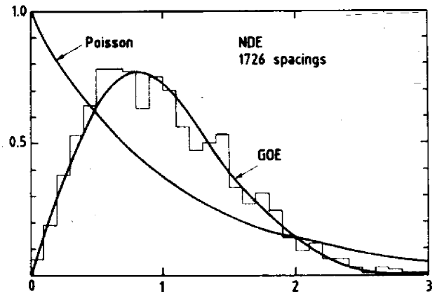
Figure 1: Nearest neighbor spacing distribution for the “Nuclear Data Ensemble” comprising 1726 spacings (histogram) versus $s=S/D$ with $D$ the mean level spacing and $S$ the actual spacing. Note the level repulsion in random matrix theory (GOE denotes the Gaussian Orthogonal random matrix Ensemble) at zero spacing as compared to the Poisson distribution. Taken from reference [14]. Used with permission.

Shortly thereafter RMT was applied to the spectra of atoms. Later on, modern laser spectroscopy has allowed a comparison with the complex spectra of polyatomic molecules. Nuclei, atoms and molecules are all examples of complex many–body systems with a large number of degrees of freedom.

2.2 Quantum chaos

It was later realized that the Wigner–Dyson ensembles could be applied to the description of chaotic quantum systems. In these, a quantum particle is reflected elastically at the boundaries of some given domain, so that the total energy is constant. In such a system, all constants of the motion (except the energy) are destroyed by randomness, and there are no stable periodic orbits. The system is referred to as a quantum billiard (see Fig. 2). Due to the shape of the domain, normally chosen to be two–dimensional, the trajectory of the particle is completely random. Such a system may have just a few degrees of freedom and may be simulated by microwave cavities. The reason is that the wave equation for the electromagnetic field in the cavity has the same form as the Schrödinger equation for a two–dimensional quantum billiard, if the geometry of the cavity and the boundary conditions are chosen appropriately. In this Schrödinger equation, the Hamiltonian for the free particle is simply the Laplace operator. With appropriate boundary conditions the system may also be equivalent to a vibrating membrane.

Figure 2: Four important billiards: the Bunimovich stadium (top left), the Sinai billiard (top right), the Pascalian snail (bottom left) and the annular billiard (bottom right). Reprinted from reference [2] with permission from authors and from Elsevier.

Spectra of such systems with up to a thousand eigenmodes have been studied experimentally (for a list of references, see [2]). The results can be interpreted in terms of classical chaos. The general picture emerging from such experiments is that if the shape of the cavity is such that the classical motion in it is integrable (regular), the spectrum behaves according to a Poisson distribution. If the corresponding classical motion is chaotic, the spectral fluctuations behave in accordance with the Wigner–Dyson ensembles. This is also the content of the famous (but unproven) Bohigas conjecture.

2.3 Mesoscopic systems, BdG and transfer matrix ensembles

A newer class of interesting quantum systems with randomness is provided by disordered metals, i.e. micrometer–sized metal grains, of which we wish to study the transport properties when the grain is connected to electron reservoirs through (ideal) leads (for a review, see [15]). Such microstructures can be fabricated in a cavity in a semiconductor. They can be made so thin that the electron gas inside them is effectively two–dimensional. Such structures are quantum systems, yet they are large enough for a statistical description to be meaningful. Therefore they are referred to as mesoscopic systems. The transmission eigenvalues related to the transfer matrix formalism determine the conductance, which is the main observable. We will discuss these systems more explicitly in the third lecture.

Disorder in such systems arises because of randomly distributed impurities in the metal. The electrons in the conduction band are scattered elastically by the resulting random potential as we apply a voltage drop across the metal sample. Such a system is called diffusive. At low temperature (below 1K), inelastic electron–phonon scattering, which changes the phases of the electrons in a random way, can be neglected. The electrons are therefore phase coherent over the length of the sample. In the diffusive regime (with the conductance decreasing linearly with sample size) we expect Wigner–Dyson statistics to apply to the spectrum of energy levels (at least up to an energy separation given by the so–called Thouless energy). The random matrix theory of quantum transport, however, deals mostly with the transmission eigenvalues. It relates the universality of transport properties (i.e., the independence of these of sample size, degree of disorder, etc.) to the universality (to be discussed) of correlation functions in random matrix theory.

The behavior of the conductance depends critically on the dimensionality of the sample. In $1d$ all states are localized and the sample is an insulator, while $d=2$ is the critical dimension and delocalization occurs for $d>2$. If the sample has the shape of a grain, it is called a quantum dot. A quantum wire is a very thin (quasi–one dimensional) metal wire with similar properties, that allows to study the scaling properties of observables related to transport as a function of the length of the wire through a generalized diffusion equation. Quasi–$1d$ wires are particularly good laboratories for testing RMT. Since they are not strictly one–dimensional, they possess a diffusive regime (cf. the comment above on dimensionality); still, non–perturbative analytical methods are applicable (scaling equation, field theoretical methods).

The phenomenon of localization occurs when the previously extended Bloch wave functions of the multiply scattered electrons are cancelled by destructive interference. This happens when the density of impurities reaches a critical value. As a consequence, the metal sample goes from being a conductor to being an insulator. In the localized (insulating) regime the conductance decays exponentially as a function of sample size and the typical length scale of the decay of electron wave functions is given by the localization length $\xi$. In the localized regime, wave functions of nearly degenerate states may have a very small overlap. As a consequence, the level repulsion typical of the Wigner–Dyson ensembles is suppressed and we expect Poisson statistics (uncorrelated eigenvalues) on length scales larger than $\xi$.

We may also consider a metal grain in which electron scattering takes place at the boundaries. In the latter case the mean free path of the electrons is large compared to the size of the system and we speak of a ballistic system. A ballistic quantum dot is very similar to a billiard and is described by Wigner–Dyson statistics (see Fig. 3).

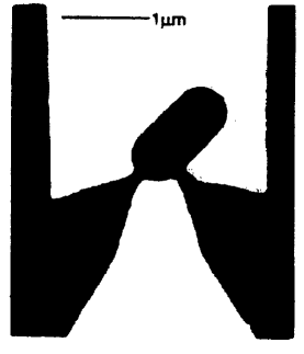
Figure 3: Electron micrograph of a quantum dot in the shape of a Bunimovich stadium, with $1~{}\mu$m bar for scale. The electrons can move in the black area. Two leads are coupled to the stadium. Reprinted with permission from ref. [16]. Copyright 2005 by the American Physical Society.

In addition to these systems, heterostructures consisting of superconductors in conjunction with normal metals are successful candidates for a random matrix theory description. In these we have particle–hole symmetry and the (first–quantized) Hamiltonians in this case are described by four new so–called Bogoliubov–de Gennes (BdG) ensembles [17].

The existence of several mesoscopic regimes (localized, diffusive, ballistic, with varying degree of disorder) enriches the phenomenology and extends the applications of RMT beyond the ones discussed for many–body and chaotic systems. In particular, the case of normal–superconducting quantum dots leads to four entirely new symmetry classes of Hamiltonians.

In mesoscopic systems, the operator that is modelled by random matrix ensembles is either the Hamiltonian or the transfer matrix. In the random Hamiltonian approach, ensemble averages are calculated in the supersymmetric formalism [18] using scattering theory. (The supersymmetric formalism is partly discussed also in [2]. In addition see [19] for QCD–related applications.) In the random transfer matrix approach, which we will discuss more explicitly later, the transmission eigenvalues determine important transport properties, of which the most central one is the conductance determined in the Landauer–Lee–Fisher theory. To every ensemble of Hamiltonians corresponds an ensemble of transfer matrices (and one of scattering matrices as well) describing the same physical system.

2.4 Field theory and chiral ensembles

Random matrices are also useful in relativistic quantum field theory. In a gauge field theory, the interactions between the gauge field and the fermions is expressed as a gauge field integration over the fermion determinant, obtained by integration over the fermionic (Grassmann) variables in the partition function. The fermion determinant involves the Dirac operator and depends on the gauge fields. This operator can also be modelled by an ensemble of random matrices. If chiral symmetry is present, these ensembles are called chiral random matrix ensembles. The matrices in these ensembles have a block–structure similar to the Dirac operator in the chiral basis, and may possess zero modes. This application of random matrix theory was developed by Verbaarschot et al. in the 1990’s (for some early work, see [20]).

The procedure of substituting the Dirac operator with a random matrix makes it possible to perform the integration over the gauge fields by integrating over the ensemble of random matrices. By using techniques borrowed from the supersymmetric formalism originally developed for scattering problems in the physics of quantum transport, one can then obtain the effective low–energy partition function in the gauge theory [21]. In the presence of spontaneous symmetry breaking, it is expressed as an integral over the Goldstone manifold (i.e. over the degrees of freedom associated with spontaneous symmetry breaking in the gauge theory). This way the symmetry breaking pattern is also obtained and in addition, sum rules for the eigenvalues of the Dirac operator can be derived. Recently, there have been interesting new developments in this field, relating the QCD partition function to integrable hierachies (for a comprehensive review with references, see the lecture series by Verbaarschot [22]).

The order parameter for the spontaneously broken phase (the quark condensate in QCD) is proportional to the density of Dirac eigenvalues at the origin of the spectrum (i.e., at zero eigenvalue). This is expressed by the Banks–Casher formula. Therefore the Dirac spectrum, and especially the regime around the origin, is of major interest. Its generic features can be studied in RMT. A wealth of numerical simulations [23] in lattice gauge theory show that data agree with RMT predictions for level correlators and low–energy sum rules for the Dirac eigenvalues. This shows that fluctuations of Dirac eigenvalues are generic and independent of details of the gauge field interactions. Two reviews with references to original work are given in [24].

Note that since these lectures are introductory, we will limit the discussion to hermitean random matrix models. Therefore we will not discuss the new developments in this field involving non–hermitean random matrices (see e.g. [25]), even though these are very intriguing as they allow a study of the case of nonzero baryon chemical potential. The same is true for the new research developments in non–hermitean random matrix theory in other branches of physics. Such applications include for instance the description of non-equilibrium processes, quantum chaotic systems with an imaginary vector potential (related to superconductivity), and neural networks.

3 What is random matrix theory?

We have established that some of the things that may make a system chaotic are: complex many–body or gauge field interactions, a random impurity potential, or irregular shape (where irregular means any shape leading to classical chaotic motion). Because of the high number of degrees of freedom or the complexity of the interactions in chaotic systems, the quantum mechanical operators whose spectra and eigenfunctions we are interested in may be unknown or inaccessible to direct calculation. Such an operator may be a Hamiltonian, a scattering or transfer matrix, or a Dirac operator, as we have seen above. These operators can be represented quantum mechanically by matrices acting on a Hilbert space of states.

In studying nuclear resonances, Wigner [13] proposed replacing the Hamiltonian of the nucleus by a random matrix taken from some well–defined ensemble. How do we determine which ensemble is appropriate? Wigner proposed choosing it so that the general global symmetries of the underlying physical problem are preserved. This means that we should choose random matrices with the same global symmetries as the physical operator we are modelling. In doing so, we will preserve the spectral properties that depend only on these symmetries. These are the aspects of the spectrum we will be able to study using RMT.

As it turns out, the gross features of the random matrix theory spectrum, like for instance the macroscopic shape of the eigenvalue density, is usually not of interest for studying the physical system, as it does not even remotely resemble the actual spectrum and is non–universal in that it depends on the choice of random matrix potential. The strength of the RMT description lies in the universal behavior of the eigenvalue correlators in a certain scaling limit. As we will see, this leads to universal spectral fluctuations that are reproduced by a multitude of physical systems in the real world, several of which we have discussed in the previous paragraph.

The statistical theory of Wigner [13] and Dyson [3] is a theory of random matrices. These are matrices with random elements chosen from some given distribution. In the applications to be discussed here, we use them to represent a quantum mechanical operator, whose eigenvalue spectrum and eigenstates are of physical interest. In the classical example of the heavy nucleus, the Schrödinger equation

$$H\Psi_{i}=E_{i}\Psi_{i}$$ (3.1)

gives the energy spectrum of the nucleus with Hamiltonian $H$. In case this Hamiltonian is unknown or too complicated, we may choose to study the eigenvalues of an appropriate ensemble of random matrices instead. The ensembles studied by Dyson in the early sixties were ensembles of scattering matrices, but the principle is the same.

The random matrix eigenvalues should behave much like the energy levels of the nucleus, if we choose our ensemble of random matrices appropriately. To achieve this we analyze the physical symmetries of the Hamiltonian and choose an ensemble of random matrices with these same symmetries. The characteristics of the spectrum that depend only on these symmetries will be present also in the spectrum of the random matrix eigenvalues. These are the universal features of the system, and they are obtained after removal of the non–universal behavior through a proper rescaling procedure. They do not depend on details of the physical interactions or, in the RMT, on the choice of RMT potential.

The number of fields where random matrix models are applied nowadays is growing fast. To convey the main ideas, we will concentrate on a few major applications.

4 Choosing an ensemble

What are the physical symmetries that determine the ensemble of random matrices? Dyson’s analysis shows that for the Hamiltonian ensembles there are three generic cases:

1) The system is invariant under time–reversal (TR) and the total spin is integer (even–spin case), or the system is invariant under time–reversal and space–rotation (SR) with no regard to the spin.

2) The system is invariant under time–reversal but with no rotational symmetry and the total spin is half–odd integer (odd–spin case).

3) The system is not time–reversal invariant.

In all these cases, the ensemble of random matrices is invariant under the automorphism

$$H\rightarrow UHU^{-1}$$ (4.1)

where $U$ is an orthogonal (case 1), unitary (case 3) or symplectic (case 2) matrix. It is this property that gives rise to the identification of the manifolds of random matrices with symmetric spaces. This identification is very useful, since it leads to the possibility of applying the known theory of symmetric spaces in physical contexts.

The properties of these ensembles are summarized in Table 1.

Table 1: Dyson’s three universality classes of random matrices. The Dyson index $\beta$ counts the number of degrees of freedom of the matrix elements (each matrix element is a real, complex or quaternion number) and is used to specify the ensemble. The ensembles are named the orthogonal, unitary or symplectic ensemble, respectively, according to the subgroup of invariance.

$\beta$	TR	SR	$H$	$U$
1	X	X	real, orthogonal	orthogonal
2		(X)	complex, hermitean	unitary
4	X		real quaternion, self-dual	symplectic

The relevant physical symmetries depend on the system under consideration. Novel ensembles not included in this classification arise if we impose additional symmetries or constraints. This is the case for the four universality classes of the Hamiltonians of normal–superconducting (NS) quantum dots (for a detailed discussion see [17]). Also here the four universality classes are distinguished by the presence or absence of TR and SR, but with the difference that the Hamiltonian possesses so–called particle–hole symmetry. As electrons tunnel through the potential barrier at the NS interface, a Cooper pair is added to, or subtracted from, the superconducting condensate. Equivalently, an electron incident on the interface is reflected as a hole (a phenomenon referred to as Andreev reflection).

Three more chiral symmetry classes are realized in chiral gauge theories. In this case the ensemble is chosen such that the chiral symmetry $[\gamma_{5},i\!\not{\!\!D}]=0$, the zero modes and possible anti–unitary symmetries $[Q,i\!\not{\!\!D}]=0$ of the Euclidean Dirac operator (where $Q$ is some anti–unitary operator) are reproduced by the ensemble. The properties of $Q$ determine if there is a basis in which the Dirac operator is real or quaternion real. In this case we also have three symmetry classes distinguished by the index $\beta$.

As we will see later, to every hamiltonian ensemble there corresponds a scattering matrix ensemble and a transfer matrix ensemble. The hamiltonian and scattering matrix ensembles of a given physical system are related to each other in a simple way: the hamiltonian ensemble is simply the algebra subspace corresponding to the compact symmetric space of the scattering matrix. Because of the way transfer matrices are defined, the ensemble of the transfer matrix of the same system is not the corresponding non–compact space. Nevertheless, it will neatly fit into the classification scheme. For scattering and transfer matrices in the theory of quantum transport we use ensembles constrained by the physical requirements of flux conservation, time–reversal symmetry, and spin–rotation. Flux conservation imposes the condition of unitarity on the scattering matrix, and determines the symmetry class of the transfer matrix too. We will discuss some explicit examples in the third lecture.

5 General definition of a matrix model

Since many of the interesting quantum operators are physical observables, we often deal with hermitean random matrices. Non–hermitean operators are also of interest. The number of fields where they are important is growing, and so is the research effort devoted to this large class of random matrix theories. Here we will only be concerned with hermitean random matrices.

A hermitean matrix model is defined by a partition function

$$Z\sim\int dH\,P(H)$$ (5.1)

where $H$ is a square $N\times N$ hermitean matrix with random elements $H_{ij}$ chosen from some given distribution. At the end of our calculation, we will take the limit $N\rightarrow\infty$ to counteract the fact that we are using, for technical reasons, a truncated Hilbert space. In equation (5.1) $P(H)$ is a probability distribution in the space of random matrices and $dH$ is an invariant measure in this space. Such a measure is required to give physical meaning to the concept of probability: $P(H)dH$ is the probability that a quantum operator in the ensemble will belong to the volume element $dH$ in the neighborhood of $H$. Since the ensemble of matrices $\{H\}$ does not in general form a group, the existence of such a measure is not entirely trivial. Dyson [3] showed that a unique invariant (Haar) measure $dH$ exists for the three ensembles discussed in the previous section.

One can show that a probability distribution of the form

$$P(H)\sim{\rm e}^{-c\,{\rm tr}V(H)}$$ (5.2)

is appropriate (see [26] for more details on this point). Note that such a weight function is needed to keep the integrals from diverging. Here $c$ is a constant and $V(H)$ is a matrix potential, typically a polynomial with a finite number of terms. The simplest choice is a quadratic potential, in which case the matrix model is called gaussian. A common choice for the Wigner–Dyson ensembles is

$$P_{\beta}(H)\sim{\rm e}^{-\frac{\beta N}{2v^{2}}{\rm tr}H^{2}}$$ (5.3)

where $v$ has the same dimension as the matrix elements of $H$. The factor in front of the potential is chosen proportional to $\beta$ for later convenience and proportional to $N$ so that the spectrum, that has support on some finite interval on the real axis, will remain bounded in the large $N$ limit. In this case the macroscopic eigenvalue spectrum is a semicircle. Such a spectrum is quite unrealistic for most physical systems, and not interesting in itself. What’s more, the macroscopic form of the spectrum depends on the form of the potential. However, the statistical eigenvalue fluctuations will turn out to be universal and independent of the matrix potential in the large–$N$ limit, if we scale the eigenvalues appropriately (a process referred to as unfolding). Our focus will be on such universal quantities.

The probability $P(H)dH$ is invariant under the automorphism

$$H\rightarrow U^{-1}HU$$ (5.4)

of the ensemble to itself, where $U$ is a unitary $N\times N$ matrix. By doing an appropriate similarity transformation (5.4) on the ensemble of random matrices, the Haar measure $dH$ and potential $V(H)$ can be expressed in terms of the eigenvectors and eigenvalues of the matrix $H$:

$$H\rightarrow U^{-1}\Lambda U$$ (5.5)

where $\Lambda$ is (block)diagonal and contains the eigenvalues. The Haar measure is then factorized as follows

$$dH=dU\,J(\{\lambda_{i}\})\prod_{i=1}^{N}d\lambda_{i}$$ (5.6)

where $dU$ depends only on the eigenvectors and can be integrated out to give a trivial constant in front of the integral. $J(\{\lambda_{i}\})$ is the Jacobian of the similarity transformation (5.4). It is given by [26]

$$J_{\beta}(\{\lambda_{i}\})\sim\prod_{i<j}|\lambda_{i}-\lambda_{j}|^{\beta}$$ (5.7)

for the Wigner–Dyson ensembles labelled by $\beta$.

For a gaussian potential $V(H)=\frac{1}{2}H^{2}$ the partition function then takes the form

$$Z_{\beta}(\{\lambda_{i}\})\sim\int P_{\beta}(\{\lambda_{i}\})\,d\lambda_{1}...d\lambda_{N}=\int\prod_{i<j}|\lambda_{i}-\lambda_{j}|^{\beta}\,{\rm e}^{-\frac{\beta N}{2v^{2}}\sum_{j=1}^{N}\lambda_{j}^{2}}\,d\lambda_{1}...d\lambda_{N}$$ (5.8)

This model is easily solvable. This is the strength of the random matrix description of disordered systems.

The Jacobian in (5.7) has the form of a Vandermonde determinant. If we rewrite eq. (5.7) so that the Jacobian is in the exponent, it gives rise to repulsive eigenvalue correlations in the form of a logarithmic pair potential. Such correlations are called geometrical, because they arise only from the Jacobian. In the absence of the invariance (5.4), the eigenvalues are uncorrelated and follow a Poisson distribution.

6 The correlators

The basis for comparing random matrix predictions to experimental or numerical measurements are the eigenvalue correlation functions. These determine the statistical properties of the ensemble.

The $k$–point correlation function $\rho_{k}(\lambda_{1},...,\lambda_{k})$ is defined as

$$\rho_{k}(\lambda_{1},...,\lambda_{k})=\frac{N!}{(N-k)!}\int\prod_{j=k+1}^{N}d\lambda_{j}P(\{\lambda_{1},...,\lambda_{N}\})$$ (6.1)

$\rho_{k}(\lambda_{1},...,\lambda_{k})d\lambda_{1}...d\lambda_{k}$ denotes the probability of finding any $k$ eigenvalues in the intervals $d\lambda_{i}$ around the points $\lambda_{i}$ ($i=1,...,k$). The 1–point function is just the density of eigenvalues.

Calculation of the $k$–point correlators can be performed exactly [26] by rewriting the Jacobian as a product of Vandermonde determinants of a set of polynomials orthogonal with respect to some measure $f(\lambda)$. This can easily be done just using the properties of determinants. For instance, for a gaussian matrix model, $f(\lambda)={\rm e}^{-\frac{\beta N}{2v^{2}}\lambda^{2}}$ and the polynomials are the Hermite polynomials:

$$\int_{-\infty}^{+\infty}H_{m}(\lambda)H_{n}(\lambda){\rm e}^{-\frac{\beta N}{2v^{2}}\lambda^{2}}d\lambda=h_{n}\delta_{mn}$$ (6.2)

where $h_{n}$ is a normalization. All the classical orthogonal polynomials appear in this context for various choices of the function $f(\lambda)$.

The procedure of calculating correlators using orthogonal polynomials was reviewed in Mehta’s book [26], and was a big step forward for random matrix theory at the time. The formula for the $k$–point correlator can be summarized by the formula

$$\rho_{\beta,k}(\lambda_{1},...,\lambda_{k})={\rm qdet}[Q_{N\beta}]$$ (6.3)

where ${\rm qdet}$ denotes a quaternion determinant. The matrix elements of $Q_{N\beta}$ are determined by universal translation invariant kernels [26] in the large $N$ limit and on the unfolded scale. Therefore, eigenvalue correlators are universal and determined only by symmetry. To obtain this universal behavior, one has to unfold the spectrum. This means rescaling the eigenvalues in such a way that they become dimensionless, by removing the dependence of the non–universal density of eigenvalues $\rho_{1}(\lambda)$. Let’s define dimensionless variables $x_{i}$ by

$$x_{i}=x_{i}(\lambda_{i})=\int_{-\infty}^{\lambda_{i}}\rho_{1}(\lambda^{\prime})d\lambda^{\prime}$$ (6.4)

The unfolded correlators are obtained by requiring that the differential probabilities should be the same in the old and in the new variables:

$$\rho_{k}(\lambda_{1},...,\lambda_{k})d\lambda_{1}...d\lambda_{k}=X_{k}(x_{1},...,x_{k})dx_{1}...dx_{k}$$ (6.5)

Note that $X_{1}(x)=1$ by construction.

In practice, however, it is sufficient to do the rescaling in a small region of the spectrum, where we are interested in studying the correlations. If this region is centered, say, at the origin, we put $z_{i}=\lambda_{i}/\Delta$ where $\Delta=\rho_{1}(0)^{-1}$ is the average level spacing at the origin (note that this quantity is a function of $N$). This amounts to magnifying the region on the scale of the average level spacing, simultaneously with taking the large $N$ limit in which the spectrum becomes dense. This so–called microscopic $k$–point function (we will call it $\rho_{S,k}(z_{1},...,z_{k})$ in accordance with standard usage) is then given by

$$\rho_{S,k}(z_{1},...,z_{k})=\begin{array}[]{c}{\rm lim}\\ {\scriptstyle N\rightarrow\infty}\end{array}\Delta^{k}\rho_{k}(\Delta z_{1},...,\Delta z_{k})$$ (6.6)

where we simultaneously take the limit $N\rightarrow\infty$, keeping the $z_{i}$ fixed. The new correlators $\rho_{S,k}(z_{1},...,z_{k})$ are independent of the random matrix potential within a large class of potentials. The microscopic spectral correlators can be measured in computer simulations (see Fig. 4 for an example).

           

Figure 4: Measurements of the spectrum of the Dirac operator in SU(2) lattice gauge theory are compared to predictions from random matrix theory. The figure shows the distribution of the smallest Dirac eigenvalue $P(\lambda_{\rm min})$, microscopic spectral density $\rho_{S}(z)$ (for a 10⁴ lattice) and the microscopic spectral two-point function $\rho_{S}(x,y)$ (for an 8⁴ lattice). The histograms represent lattice SU(2) data; the dashed lines are analytical predictions from RMT. Reprinted with permission from ref. [27]. Copyright 2005 by the American Physical Society.

The cluster functions are relevant for computing spectral observables. A cluster function is defined as the connected part of a general $k$–point function. (For comparison, for an uncorrelated (Poisson) distribution, the connected part vanishes.) For instance, before unfolding the two–point function takes the form

$$\rho_{2,\beta}(\lambda_{1},\lambda_{2})=\rho_{1,\beta}(\lambda_{1})\rho_{1,\beta}(\lambda_{2})-T_{2,\beta}(\lambda_{1},\lambda_{2})$$ (6.7)

where the 2–level cluster function is given by $T_{2,\beta}(\lambda_{1},\lambda_{2})$. After unfolding, both the 2–point function and the 2–point cluster function depend only on the difference $r=x_{1}-x_{2}$, and we have

$$X_{2,\beta}(r)=1-Y_{2,\beta}(r)$$ (6.8)

where $X_{2,\beta}(r)$ is the unfolded 2–point function and $Y_{2,\beta}(r)$ the unfolded cluster function.

7 Spectral observables

In comparing random matrix theory with experimental and numerical results, we need to transform the $k$–point functions into statistical spectral observables that can be compared to data.

In this paragraph we closely follow ref. [2]. We will consider an energy spectrum that is the result of a measurement or of a numerical calculation. The measured values (and the random matrix eigenvalues) will be denoted by an ordered sequence $\{E_{1},...,E_{N}\}$. We define a spectral function

$$S(E)=\sum_{n=1}^{N}\delta(E-E_{n})$$ (7.1)

and a cumulative spectral function or staircase function

$$\eta(E)=\int S(E^{\prime})dE^{\prime}=\sum_{n=1}^{N}\theta(E-E_{n})$$ (7.2)

where $\theta$ is the step function. The cumulative spectral function contains a smooth and a fluctuating part:

$$\eta(E)=\xi(E)+\eta_{fl}(E)$$ (7.3)

where $\xi(E)$ is the cumulative mean level density

$$\xi=\xi(E)=\int_{-\infty}^{E}\rho_{1}(E^{\prime})dE^{\prime}$$ (7.4)

To obtain the smooth part of the experimentally obtained staircase function, one may fit a polynomial to it (see Fig. 5).

Figure 5: Example of an experimentally obtained staircase function for a spectrum of 1428 elastomechanical eigenfrequencies of a resonating quartz block. Due to the high number of levels, the staircase function appears as a smooth line. The smooth part $\xi(E)$ is a polynomial whose coefficients were found by a fit. The bottom part shows a small section of the staircase function. Adapted from Ellegaard et al. [28] by Guhr, Müller–Groeling and Weidenmüller [2]. Copyright 2005 by the American Physical Society and with permission from Elsevier.

The unfolding procedure is identical to the one we performed in RMT in the previous paragraph. After unfolding, $\xi_{i}=\xi(E_{i})$, the staircase function is expressed as

$$\hat{\eta}(\xi)=\xi+\hat{\eta}_{fl}(\xi)$$ (7.5)

where $\xi$ is the dimensionless variable defined in (7.4). Note that the mean level density of the unfolded spectrum (i.e. the derivative of the smooth part of the step function) is unity, as we have removed the non–universal dependence.

We will now discuss how a few spectral observables are obtained from the correlation functions.

To study long–range correlations a common statistic is the level number variance $\Sigma^{2}(L)$. If $\hat{\eta}$ denotes the number of levels in the interval $[\xi,\xi+L]$ in the unfolded spectrum, the number variance is defined by

$$\Sigma^{2}(L)=\langle\hat{\eta}^{2}\rangle-\langle\hat{\eta}\rangle^{2}=\langle\hat{\eta}^{2}\rangle-L^{2}$$ (7.6)

where the angular brackets $\langle...\rangle$ denote the average with respect to $\xi$. In an interval of length $L$ one expects on average $L\pm\sqrt{\Sigma^{2}(L)}$ levels.

The number variance is given in terms of correlators by

$$\Sigma_{\beta}^{2}(L)=L-2\int_{0}^{L}(L-r)Y_{2,\beta}(r)\,dr$$ (7.7)

where $Y_{2,\beta}(r)$ is the unfolded 2–level cluster function.

Another long–range statistic is the spectral rigidity $\Delta_{3}$. It is defined as the least square deviation of the unfolded cumulative spectral function (staircase function) from the best fit to a straight line:

$$\Delta_{3}(L)=L^{-1}{\Big{\langle}}\begin{array}[]{c}{\rm min}\\ a,b\end{array}\int_{\xi}^{\xi+L}{\Big{(}}\hat{\eta}(\xi^{\prime})-(a\xi^{\prime}+b){\Big{)}}^{2}\,d\xi^{\prime}{\Big{\rangle}}$$ (7.8)

where, like in the number variance, the angular brackets $\langle...\rangle$ denote the average with respect to $\xi$. The spectral rigidity can similarly to $\Sigma^{2}(L)$ be expressed as an integral involving $Y_{2}(r)$.

To study fluctuations in the spectrum on a short scale (a few level spacings) we can study the nearest neighbor spacing distribution $p(s)$. This is the probability density for two neighboring levels $\xi_{n}$ and $\xi_{n+1}$ being a distance $s$ apart. The calculation of $p(s)$ is non–trivial and involves all correlation functions $\rho_{k}$ with $k\geq 2$. An excellent approximation is given by the Wigner surmise:

$$p_{\beta}(s)=a_{\beta}s^{\beta}{\rm exp}(-b_{\beta}s^{2})$$ (7.9)

where $a_{\beta}$, $b_{\beta}$ are $\beta$–dependent constants. Note the level repulsion factor $s^{\beta}$ at small $s$. See Fig. 6 for an example of measurements of these statistical observables.

Figure 6: Statistical observables in the Dirac spectrum of SU(2) gauge theory. The figures show a comparison of lattice data and RMT predictions for the number variance $\Sigma_{2}$, the $\Delta_{3}$ statistic, and the nearest neighbor spacing distribution $p(s)$. The two columns show different implementations of fermions on the lattice (left: Wilson fermions, right: Kogut-Susskind fermions). GOE, GUE and GSE stand for the Gaussian Orthogonal, Unitary, and Symplectic Ensemble, respectively. Reprinted from [29] with permission from Elsevier.

For comparison of measurements to RMT predictions to make sense, we have to make the assumption of ergodicity. This means that we assume that the ensemble average in the theoretical prediction of RMT is equal to the running average over the sequence of measurements on a single sample:

$$\langle f(E)\rangle_{ens}=\langle f(E)\rangle_{meas}$$ (7.10)

where $f(E)$ denotes any function of the eigenvalues.

The observed spectral fluctuations in the systems we have discussed in the introduction show, in many instances, an impressive agreement with random matrix theory predictions.

8 Lie groups, algebras, and root lattices

In this lecture we will first present some preliminary material leading up to the definition of symmetric spaces. Assuming that most of the audience is more familiar with this concept than the average physicist, we will be as brief as possible.

As already mentioned, the reason we are interested in symmetric spaces in connection with RMT is that random matrix ensembles are identified with symmetric spaces. As we will see, symmetric spaces (SS) have well–known properties [6, 7] and much of the theory for SS can be used in physical problems where RMT is applicable. We will give a few examples of such usage in the next lecture.

We will start by reminding the reader of some basic definitions concerning Lie algebras and root spaces. A Lie algebra ${\bf G}$ is a linear vector space over a field $F$. Multiplication in the Lie algebra is given by the Lie bracket $[X,Y]$. It has the following properties:

[1] If $X$, $Y\in{\bf G}$, then $[X,Y]\in{\bf G}$,
[2] $[X,\alpha Y+\beta Z]=\alpha[X,Y]+\beta[X,Z]$ for $\alpha$, $\beta\in F$,
[3] $[X,Y]=-[Y,X]$,
[4] $[X,[Y,Z]]+[Y,[Z,X]]+[Z,[X,Y]]=0$ (the Jacobi identity).

The algebra ${\bf G}$ generates a group through the exponential mapping. A general group element is

$$M={\rm exp}\left(\sum_{i}t^{i}X_{i}\right);\ \ \ \ t^{i}\in F,\ X_{i}\in{\bf G}$$ (8.1)

where $t_{i}$ are parameters (coordinates). We define a mapping ${\rm ad}X$ from the Lie algebra to itself by ${\rm ad}X:Y\rightarrow[X,Y]$. The mapping $X\rightarrow{\rm ad}X$ is a representation of the Lie algebra called the adjoint representation. It is easy to check that it is an automorphism (i.e. that it preserves algebraic operations): it follows from the Jacobi identity that $[{\rm ad}X_{i},{\rm ad}X_{j}]={\rm ad}[X_{i},X_{j}]$. Suppose we choose a basis $\{X_{i}\}$ for ${\bf G}$. Then

$${\rm ad}X_{i}(X_{j})=[X_{i},X_{j}]=C^{k}_{ij}X_{k}$$ (8.2)

where we sum over $k$. The $C^{k}_{ij}$ are real structure constants. The structure constants define the matrices $M$ of the adjoint representation through $(M_{i})_{jk}=C^{j}_{ik}$.

An ideal ${\bf I}$ is a subalgebra such that $[{\bf G},{\bf I}]\subset{\bf I}$. A simple Lie algebra has no proper ideal. The semisimple algebras are built from the simple ones. In any simple algebra there are two kinds of generators.

(1) There is a maximal abelian subalgebra, called the Cartan subalgebra ${\bf H_{0}}=\{H_{1},...,H_{r}\}$ such that

$$[H_{i},H_{j}]=0$$ (8.3)

If we represent each element of the Lie algebra by an $n\times n$ matrix, then $[H_{i},H_{j}]=0$ means the matrices $H_{i}$ can all be diagonalized simultaneously. Their eigenvalues $\mu_{i}$ are given by

$$H_{i}|\mu\rangle=\mu_{i}|\mu\rangle$$ (8.4)

where the eigenvectors are labelled by the weight vectors $\mu=(\mu_{1},...,\mu_{r})$. A positive weight is a weight whose first non–zero component is positive.

(2) There are raising and lowering operators denoted $E_{\alpha}$ such that

$$[H_{i},E_{\alpha}]=\alpha_{i}E_{\alpha},\ \ \ \ \ [E_{\alpha},E_{-\alpha}]=\alpha_{i}H_{i}$$ (8.5)

Here $\alpha$ is an $r$–dimensional vector called a root: $\alpha=(\alpha_{1},...,\alpha_{r})$ and $r$ is the rank of the algebra. For each root $\alpha_{i}$, there is another root $-\alpha_{i}$ and a corresponding eigenoperator $E_{-\alpha}$. The roots form a lattice in the space dual to the Cartan subalgebra. A subset of the positive roots span the root lattice. These are the simple roots. Their number is equal to $r$, the rank of the algebra. All the weights of a representation can be obtained by acting on the highest weight with lowering operators in all possible ways.

One can prove the following relation between roots and weights:

$$\frac{2\alpha\cdot\mu}{\alpha^{2}}=-(p-q)$$ (8.6)

where $p$, $q$ are positive integers such that $E_{\alpha}|\mu+p\alpha\rangle=0$, $E_{-\alpha}|\mu-q\alpha\rangle=0$, i.e. they define the distance of $|\mu\rangle$ to the upper and lower end of the ladder.

Eq. (8.6) implies that the possible angle between two root vectors of a simple Lie algebra is limited to multiples of $\frac{\pi}{6}$ and $\frac{\pi}{4}$. Therefore, there is a finite set of possible root lattices. Equation (8.6) permits a classification of all complex semisimple algebras. The classical Lie algebras ${\bf SU(n+1,C)}$, ${\bf SO(2n+1,C)}$, ${\bf Sp(2n,C)}$ and ${\bf SO(2n,C)}$ correspond to root systems $A_{n}$, $B_{n}$, $C_{n}$, and $D_{n}$, respectively. In addition there are five exceptional algebras, but these are not relevant for random matrix theory because they have a finite $n$.

The root systems for these four infinite series of classical non–exceptional Lie groups can be characterized as follows [30] (denote the $r$–dimensional space spanned by the roots by ${\cal V}$ and let $\{e_{1},...e_{n}\}$ be a canonical basis in ${\bf R}^{n}$):

$A_{n-1}$: Let ${\cal V}$ be the hyperplane in ${\bf R}^{n}$ that passes through the points $(1,0,0,...0)$, $(0,1,0,...,0)$, …, $(0,0,...,0,1)$ (the endpoints of the $e_{i}$, $i=1,...,n$). Then the root lattice contains the vectors $\{e_{i}-e_{j},i\neq j\}$.

$B_{n}$: Let ${\cal V}$ be ${\bf R}^{n}$; then the roots are $\{\pm e_{i},\pm e_{i}\pm e_{j},i\neq j\}$.

$C_{n}$: Let ${\cal V}$ be ${\bf R}^{n}$; then the roots are $\{\pm 2e_{i},\pm e_{i}\pm e_{j},i\neq j\}$.

$D_{n}$: Let ${\cal V}$ be ${\bf R}^{n}$; then the roots are $\{\pm e_{i}\pm e_{j},i\neq j\}$.

The root lattice $BC_{n}$, that we will discuss in conjunction with restricted root systems, is the union of $B_{n}$ and $C_{n}$. It is characterized as follows:

$BC_{n}$: Let ${\cal V}$ be ${\bf R}^{n}$; then the roots are $\{\pm e_{i},\pm 2e_{i},\pm e_{i}\pm e_{j},i\neq j\}$.

Roots of length 1, $\sqrt{2}$, and 2 are called short, ordinary, and long roots, respectively. Each of the complex algebras in general has several real forms associated with it. We will define these shortly. Eq. (8.6) expresses invariance of the root lattice under reflections in the hyperplanes orthogonal to the roots (the Weyl group). If $\mu$ is a weight or root, so is $\mu^{\prime}$:

$$\mu^{\prime}=\mu-\frac{2(\alpha\cdot\mu)}{\alpha^{2}}\alpha$$ (8.7)

The relation (8.6) determines the highest weights of all irreducible representations. Setting $p=0$, choosing a positive integer $q$, and letting $\alpha$ run through the simple roots, $\alpha=\alpha^{i}$ ($i=1,...,r$), we find the highest weights $\mu^{i}$ of all the irreducible representations corresponding to the given value of $q$ [30].

9 Cosets

In general, a symmetric space can be represented as a coset space of some Lie group $G$ with respect to a symmetric subgroup $H$. The (left) coset space $G/H$ is the set of subsets of $G$ of the form $gH$ ($g\in G$):

$$G=g_{0}H+g_{1}H+...+g_{n}H$$ (9.1)

Every element $g\in G$ can be written uniquely as $g=g_{i}h_{j}$ for some $g_{i}\in G$ and some $h_{j}\in H$. The coset can be identified with the set of group operations $\{g_{0},...,g_{n}\}$. The coset corresponds to a manifold of dimension ${\rm dim}G-{\rm dim}H$, as we will see in the example below.

Suppose $G$ is represented by matrices acting transitively on a space $V$ ($Gv=V$ for any $v\in V$) and $Hv_{0}=v_{0}$ for some $v_{0}$ (then $H$ is called the isotropy subgroup at the point $v_{0}$). Then there is one–to–one correspondence between the elements in $V$ and those in $G/H$: $gHv_{0}=gv_{0}=v$.

Example: The $SO(2)$ subgroup of $SO(3)$ is the isotropy subgroup at the north pole of a unit 2–sphere imbedded in 3–dimensional space, since it keeps this point fixed. On the other hand, the north pole is mapped onto any point on the surface of the sphere by elements of the coset $SO(3)/SO(2)$.

The ${\bf SU(3)}$ algebra is defined by the commutation relations

$$[L_{i},L_{j}]=\frac{1}{2}\epsilon_{ijk}L_{k}$$ (9.2)

where $\frac{1}{2}\epsilon_{ijk}$ are structure constants. A matrix representation of this algebra is given by

$$L_{1}=\frac{1}{2}\left(\begin{array}[]{ccc}0&0&0\\ 0&0&1\\ 0&-1&0\end{array}\right),\ \ \ \ L_{2}=\frac{1}{2}\left(\begin{array}[]{ccc}0&0&1\\ 0&0&0\\ -1&0&0\end{array}\right),\ \ \ \ L_{3}=\frac{1}{2}\left(\begin{array}[]{ccc}0&1&0\\ -1&0&0\\ 0&0&0\end{array}\right)$$ (9.3)

The subgroup $SO(2)$ is generated by $L_{3}$. This subgroup keeps the north pole fixed:

$${\rm exp}(t^{3}L_{3})\left(\begin{array}[]{c}0\\ 0\\ 1\end{array}\right)=\left(\begin{array}[]{c}0\\ 0\\ 1\end{array}\right)$$ (9.4)

The remaining group generators define the coset space $SO(3)/SO(2)$. In terms of the real coordinates $t^{1}$, $t^{2}$, an element in this coset space takes the form

$$\begin{array}[]{l}M={\rm exp}\left(\sum_{i=1}^{2}t^{i}L_{i}\right)\\ \\ =\left(\begin{array}[]{ccc}1+(t^{2})^{2}\frac{({\rm cos}\sqrt{(t^{1})^{2}+(t^{2})^{2}}-1)}{(t^{1})^{2}+(t^{2})^{2}}&t^{1}t^{2}\frac{({\rm cos}\sqrt{(t^{1})^{2}+(t^{2})^{2}}-1)}{(t^{1})^{2}+(t^{2})^{2}}&t^{2}\frac{{\rm sin}\sqrt{(t^{1})^{2}+(t^{2})^{2}}}{\sqrt{(t^{1})^{2}+(t^{2})^{2}}}\\ t^{1}t^{2}\frac{({\rm cos}\sqrt{(t^{1})^{2}+(t^{2})^{2}}-1)}{(t^{1})^{2}+(t^{2})^{2}}&1+(t^{1})^{2}\frac{({\rm cos}\sqrt{(t^{1})^{2}+(t^{2})^{2}}-1)}{(t^{1})^{2}+(t^{2})^{2}}&t^{1}\frac{{\rm sin}\sqrt{(t^{1})^{2}+(t^{2})^{2}}}{\sqrt{(t^{1})^{2}+(t^{2})^{2}}}\\ -t^{2}\frac{{\rm sin}\sqrt{(t^{1})^{2}+(t^{2})^{2}}}{\sqrt{(t^{1})^{2}+(t^{2})^{2}}}&-t^{1}\frac{{\rm sin}\sqrt{(t^{1})^{2}+(t^{2})^{2}}}{\sqrt{(t^{1})^{2}+(t^{2})^{2}}}&{\rm cos}\sqrt{(t^{1})^{2}+(t^{2})^{2}}\end{array}\right)\\ \\ \equiv\left(\begin{array}[]{ccc}.&.&x\\ .&.&y\\ .&.&z\end{array}\right);\ \ \ \ \ x^{2}+y^{2}+z^{2}=1\end{array}$$

The last equation is the equation for a 2–sphere. When the coset space representative $M$ acts on the north pole the orbit is exactly the 2–sphere:

$$M\left(\begin{array}[]{c}0\\ 0\\ 1\end{array}\right)=\left(\begin{array}[]{ccc}.&.&x\\ .&.&y\\ .&.&z\end{array}\right)\left(\begin{array}[]{c}0\\ 0\\ 1\end{array}\right)=\left(\begin{array}[]{c}x\\ y\\ z\end{array}\right)$$ (9.5)

Because of this one–to–one correspondence, the coset space $SO(3)/SO(2)$ can be identified with a unit 2–sphere imbedded in 3–dimensional space.

10 Symmetric spaces

Suppose ${\bf G}$ is a compact simple Lie algebra. A linear automorphism $\sigma\neq 1$ of the Lie algebra ${\bf G}$ onto itself such that $\sigma^{2}=1$ is called an involutive automorphism or involution. This means the eigenvalues of $\sigma$ are $\pm 1$, and $\sigma$ splits the algebra ${\bf G}$ into orthogonal eigensubspaces corresponding to these eigenvalues: ${\bf G}={\bf K}\oplus{\bf P}$ where

$$\sigma(X)=X\ \ {\rm for}\ \ X\in{\bf K},\ \ \sigma(X)=-X\ \ {\rm for}\ \ X\in{\bf P}$$ (10.1)

${\bf K}$ is a subalgebra, but ${\bf P}$ is not. From eq. (10.1), the following commutation relations hold:

$$[{\bf K},{\bf K}]\subset{\bf K},\ \ [{\bf K},{\bf P}]\subset{\bf P},\ \ [{\bf P},{\bf P}]\subset{\bf K}$$ (10.2)

A subalgebra ${\bf K}$ satisfying (10.2) is called symmetric. If we now multiply the elements in ${\bf P}$ by $i$ (this is called the “Weyl unitary trick”), we construct a new noncompact algebra ${\bf G^{*}}={\bf K}\oplus i{\bf P}$. This is called a Cartan decomposition of ${\bf G^{*}}$, and ${\bf K}$ is a maximal compact subalgebra. The coset spaces $G/K$ and $G^{*}/K$ are symmetric spaces of compact and non–compact type, respectively.

Example: Suppose $G=SU(3,C)$, the group of $3\times 3$ unitary complex matrices with unit determinant. The algebra of this group consists of eight complex antihermitean traceless matrices $X_{i}$, $i=1,...,8$. Let us take a representation $X_{i}=iT_{i}$ where $T_{i}$ denote the Gell–Mann matrices known to physicists.

An involution that splits the ${\bf SU(3,C)}$ algebra in two subspaces ${\bf K}$, ${\bf P}$ defined as above is given by complex conjugation $\sigma=K$. This involution splits the algebra $\{X_{1},...X_{8}\}$ into real and pure imaginary matrices. In the Gell–Mann representation,

$$\begin{array}[]{l}{\bf K}=\{X_{2},X_{5},X_{7}\}=\left\{\frac{1}{2}\left(\begin{array}[]{ccc}0&1&0\\ -1&0&0\\ 0&0&0\end{array}\right),\frac{1}{2}\left(\begin{array}[]{ccc}0&0&1\\ 0&0&0\\ -1&0&0\end{array}\right),\frac{1}{2}\left(\begin{array}[]{ccc}0&0&0\\ 0&0&1\\ 0&-1&0\end{array}\right)\right\}\\ \\ {\bf P}=\{X_{1},X_{3},X_{4},X_{6},X_{8}\}\\ \\ =\left\{\frac{i}{2}\left(\begin{array}[]{ccc}0&1&0\\ 1&0&0\\ 0&0&0\end{array}\right),\frac{i}{2}\left(\begin{array}[]{ccc}1&0&0\\ 0&-1&0\\ 0&0&0\end{array}\right),\frac{i}{2}\left(\begin{array}[]{ccc}0&0&1\\ 0&0&0\\ 1&0&0\end{array}\right),\frac{i}{2}\left(\begin{array}[]{ccc}0&0&0\\ 0&0&1\\ 0&1&0\end{array}\right),\frac{i}{2\sqrt{3}}\left(\begin{array}[]{ccc}1&0&0\\ 0&1&0\\ 0&0&-2\end{array}\right)\right\}\end{array}\\ \\$$

${\bf K}$ is the compact subalgebra ${\bf SO(3,R)}$ consisting of real, skew–symmetric and traceless matrices (this can easily be checked by putting $X_{2}\equiv L_{3}$, $X_{5}\equiv L_{2}$, $X_{7}\equiv L_{1}$ and comparing with the $SO(3)$ commutation relations $[L_{i},L_{j}]=\frac{1}{2}\epsilon_{ijk}L_{k}$), and ${\bf P}$ is the subspace of matrices of the form $iT$, where $T$ is real, symmetric, and traceless. The Cartan subalgebra is given by $\{X_{3},X_{8}\}\subset{\bf P}$.

By the Weyl unitary trick we now obtain from ${\bf G}$ the non–compact algebra ${\bf G^{*}}={\bf K}\oplus i{\bf P}$, where $i{\bf P}$ is a subspace of real, symmetric, and traceless matrices $-T$. The entire Lie algebra ${\bf G^{*}}$ consists of $3\times 3$ real matrices of zero trace, and generates the linear group of transformations $SL(3,R)$.

The coset space $G/K=SU(3,C)/SO(3,R)$ is a symmetric space of compact type, and the related symmetric space of non–compact type is $G^{*}/K=SL(3,R)/SO(3,R)$.

Note that the tangent space of $G/K$ (or $G^{*}/K$) at the origin (identity element) is spanned by the subspace ${\bf P}$ (or $i{\bf P}$, respectively) of the algebra. Let’s denote by $P={\rm e}^{\bf P}$ the exponential of any point in the algebra subspace spanned by the set ${\bf P}$ (such a point is a linear combination of the generators in this subspace). When $K$ is a connected subgroup, $P$ is isomorphic to $G/K$. In general $P$ is not a subgroup. However, one can show that if $p\in P$, then also $p^{\prime}=kpk^{-1}\in P$. This defines a transitive group action on $P$. Also, if $K$ is compact, every $p\in P$ is conjugate with some element in the Cartan subalgebra:

$$p=khk^{-1}$$ (10.3)

This is called spherical decomposition. It defines the angular coordinate $k$ and the spherical radial coordinate $h$ of the point $p\in P$. In plain language, every matrix in the coset space $G/K$ or $G^{*}/K$ can be diagonalized by a similarity transformation by the subgroup $K$.

Example: In the adjoint representation, which has the same dimension as the group, the complex symmetric matrices in $G/K$ $=SU(3,C)/SO(3)$ $\simeq P={\rm e}^{\bf P}$ can be diagonalized by the group $K=SO(3)$ to the form

$$p=khk^{-1};\ \ \ \ h={\rm e}^{i{\bf t\cdot H}}==\left(\begin{array}[]{ccccccc}1&...&&&&&\\ .&1&&&&&\\ .&&{\rm e}^{i{\bf t\cdot\alpha}}&&&&\\ &&&{\rm e}^{-i{\bf t\cdot\alpha}}&&&\\ &&&&{\rm e}^{i{\bf t\cdot\beta}}&&\\ &&&&&\ddots&\\ &&&&&&{\rm e}^{-i{\bf t\cdot\gamma}}\end{array}\right)$$ (10.4)

where we have written the factor of $i$ multiplying the generators in the Cartan subalgebra explicitly in the exponent ($X_{3}\equiv iH_{1},\ X_{8}\equiv iH_{2}$). The vectors $\pm{\bf\alpha},\ \pm{\bf\beta},\ \pm{\bf\gamma}$ are the three pairs of roots of $SU(3)$ (these form a regular hexagon in the plane) and the diagonal elements equal to 1 are the exponentials of the zero roots corresponding to the two operators in the Cartan subalgebra.

11 The metric on a Lie algebra

A metric tensor can be defined on a Lie algebra. This will be useful for defining the curvature of symmetric spaces. Let $\{X_{i}\}$ be a basis for the Lie algebra ${\bf G}$ and let $C_{ij}^{k}$ denote the structure constants in this basis. The metric tensor on the algebra may be defined by the Killing form $K(X_{i},X_{j})$

$$g_{ij}=K(X_{i},X_{j})\equiv{\rm tr}({\rm ad}X_{i}{\rm ad}X_{j})=C^{r}_{is}C^{s}_{jr}$$ (11.1)

The Killing form is symmetric and bilinear. According to Cartan, the Killing form is non–degenerate for a semisimple algebra. This means that ${\rm det}g_{ij}\neq 0$, so that the inverse of $g_{ij}$, denoted by $g^{ij}$, exists. Since it is also real and symmetric, it can be reduced to canonical diagonal form $g_{ij}={\rm diag}(-1,...,-1,1,...,1)$.

According to a theorem by Weyl, a simple Lie group $G$ is compact, if and only if the Killing form on ${\bf G}$ is negative definite. Otherwise it is non–compact.

Example: We have already written down the commutation relations of the compact group $SO(3,R)$ in the form $[L_{i},L_{j}]=C_{ij}^{k}L_{k}=\frac{1}{2}\epsilon_{ijk}L_{k}$. We can renormalize the generators so that the entries of the metric are unity. The commutation relations then take the form

$$\begin{array}[]{c}[\tilde{L}_{1},\tilde{L}_{2}]=-\frac{1}{\sqrt{2}}\tilde{L}_{3},\ \ \ \ \ \ \ [\tilde{L}_{2},\tilde{L}_{3}]=-\frac{1}{\sqrt{2}}\tilde{L}_{1},\ \ \ \ \ \ \ [\tilde{L}_{3},\tilde{L}_{1}]=-\frac{1}{\sqrt{2}}\tilde{L}_{2}\end{array}$$ (11.2)

We can read off the structure constants and then, using eq. (11.1), compute the components of the Killing form. In this normalization it is

$$g_{ij}=\left(\begin{array}[]{ccc}-1&&\\ &-1&\\ &&-1\end{array}\right)$$ (11.3)

(In the unrenormalized form it is $g_{ij}=-\frac{1}{2}\delta_{ij}$.) This is the metric in the $SO(3)$ algebra. It is negative, because the group is compact.

The generators of the non–compact group $SO(2,1;R)$ obey the commutation relations

$$\begin{array}[]{c}[\Sigma_{1},\Sigma_{2}]=-\frac{1}{\sqrt{2}}\Sigma_{3},\ \ \ \ \ \ \ [\Sigma_{2},\Sigma_{3}]=-\frac{1}{\sqrt{2}}\Sigma_{1},\ \ \ \ \ \ \ [\Sigma_{3},\Sigma_{1}]=\frac{1}{\sqrt{2}}\Sigma_{2}\end{array}$$ (11.4)

In the same way, using again eq. (11.1) we compute the matrix elements $g_{ij}$. The result is

$$g_{ij}=\left(\begin{array}[]{ccc}1&&\\ &1&\\ &&-1\end{array}\right)$$ (11.5)

we have labelled the rows and columns in the order 3,1,2. The generator $\Sigma_{2}$ makes up the compact subalgebra ${\bf K}$.

12 The metric on a symmetric space

The definition of the metric can be extended to an arbitrary point of a symmetric space. At the origin, the metric is defined by restricting the metric in the algebra to the tangent space (remember that the latter is spanned by the generators in the subspace ${\bf P}$ or $i{\bf P}$ of the whole algebra ${\bf G}$ or ${\bf G^{*}}$).

Example: The metric in the subspace ${\bf P}$ of ${\bf SO(3,R)}$ is obtained by excluding the row and column corresponding to the generator in ${\bf K}$, keeping the ones in ${\bf P}$:

$$g_{ij}=\left(\begin{array}[]{cc}-1&\\ &-1\end{array}\right)$$ (12.1)

Similarly, the metric in the subspace $i{\bf P}$ of ${\bf SO(2,1;R)}$ is obtained by excluding the row and column corresponding to the compact generator in ${\bf K}$ and keeping the ones in $i{\bf P}$:

$$g_{ij}=\left(\begin{array}[]{cc}1&\\ &1\end{array}\right)$$ (12.2)

Since the group acts transitively on the symmetric space, we can then use a group transformation to map the metric to an arbitrary point of the SS, using the invariance of the line element in local coordinates given by $ds^{2}=g_{ij}dx^{i}dx^{j}$.

Note that if a positive metric is required on a compact symmetric space, we can use minus the Killing form, which sometimes is more natural.

Example: The line element $ds^{2}$ on the radius–1 2–sphere isomorphic to the symmetric space $SO(3,R)/SO(2)$ in polar coordinates is $ds^{2}=d\theta^{2}+{\rm sin}^{2}\theta\,d\phi^{2}$. The metric at the point $(\theta,\phi)$ is

$$g_{ij}=\left(\begin{array}[]{cc}1&0\\ 0&{\rm sin}^{2}\theta\end{array}\right),\ \ \ \ \ \ \ g^{ij}=\left(\begin{array}[]{cc}1&0\\ 0&{\rm sin}^{-2}\theta\end{array}\right)$$ (12.3)

where the rows and columns are labelled in the order $\theta$, $\phi$.

The line element $ds^{2}$ on the hyperboloid $SO(2,1;R)/SO(2)$ in polar coordinates is $ds^{2}=d\theta^{2}+{\rm sinh}^{2}\theta\,d\phi^{2}$. The metric at the point $(\theta,\phi)$ is

$$g_{ij}=\left(\begin{array}[]{cc}1&0\\ 0&{\rm sinh}^{2}\theta\end{array}\right),\ \ \ \ \ \ \ g^{ij}=\left(\begin{array}[]{cc}1&0\\ 0&{\rm sinh}^{-2}\theta\end{array}\right)$$ (12.4)

13 Real forms and the metric

The form of the metric depends on the basis of the algebra. A complex Lie algebra ${\bf G^{C}}$ is given by

$${\bf G^{C}}=\sum_{i}c^{i}H_{i}+\sum_{\alpha}c^{\alpha}E_{\alpha}\ \ \ \ \ \ \ (c^{i},\ c^{\alpha}\ {\rm complex})$$ (13.1)

where ${\bf H_{0}}=\{H_{i}\}$ is the Cartan subalgebra and $\{E_{\pm\alpha}\}$ are the pairs of raising and lowering operators. A real form of the same algebra is obtained by taking the coordinates $c^{i}$, $c^{\alpha}$ to be real numbers, i.e.

$${\bf G}=\sum_{i}c^{i}H_{i}+\sum_{\alpha}c^{\alpha}E_{\alpha}\ \ \ \ \ \ \ (c^{i},\ c^{\alpha}\ {\rm real})$$ (13.2)

We can choose different basis vectors in this real algebra. The form of the metric will change accordingly.

The metric corresponding to the basis $\{H_{i},\pm E_{\alpha}\}$ is not diagonal. It has the form

$$g_{ij}=\left(\begin{array}[]{cccccccc}1&&&&&&&\\ &\ddots&&&&&&\\ &&1&&&&&\\ &&&0&1&&&\\ &&&1&0&&&\\ &&&&&\ddots&&\\ &&&&&&0&1\\ &&&&&&1&0\end{array}\right)$$ (13.3)

By recombining the basis vectors into

$${\bf K}=\left\{\frac{(E_{\alpha}-E_{-\alpha})}{\sqrt{2}}\right\},\ \ \ \ \ \ \ i{\bf P}=\left\{H_{i},\frac{(E_{\alpha}+E_{-\alpha})}{\sqrt{2}}\right\}$$ (13.4)

the metric takes the diagonal form

$$g_{ij}=\left(\begin{array}[]{cccccccc}1&&&&&&&\\ &\ddots&&&&&&\\ &&1&&&&&\\ &&&1&0&&&\\ &&&0&-1&&&\\ &&&&&\ddots&&\\ &&&&&&1&0\\ &&&&&&0&-1\end{array}\right)$$ (13.5)

This is called the normal real form with a diagonal metric. Here the labelling of the rows and columns is such that entries with a minus sign correspond to the generators of the compact subalgebra ${\bf K}$, the first $r$ entries equal to $+1$ correspond to the Cartan subalgebra, and the remaining ones to the operators in $i{\bf P}$ not in the Cartan subalgebra.

The compact real form is obtained from the normal real form by the Weyl unitary trick in reverse. That is, we choose the basis to be

$${\bf K}=\left\{\frac{(E_{\alpha}-E_{-\alpha})}{\sqrt{2}}\right\},\ \ \ \ \ \ \ {\bf P}=\left\{iH_{i},\frac{i(E_{\alpha}+E_{-\alpha})}{\sqrt{2}}\right\}$$ (13.6)

The metric tensor is then

$$g_{ij}=\left(\begin{array}[]{cccc}-1&&&\\ &-1&&\\ &&\ddots&\\ &&&-1\\ \end{array}\right)$$ (13.7)

Example: We will use as an example the well–known ${\bf SU(2,C)}$ algebra with Cartan subalgebra ${\bf H_{0}}=\{J_{3}\}$ and raising and lowering operators $\{J_{\pm}\}$.

$$\begin{array}[]{c}J_{3}=\frac{1}{2\sqrt{2}}\tau_{3},\ \ \ \ \ \ \ J_{\pm}=\frac{1}{4}(\tau_{1}\pm i\tau_{2})\end{array}$$ (13.8)

where

$$\tau_{3}=\left(\begin{array}[]{cc}1&0\\ 0&-1\end{array}\right),\ \ \ \ \tau_{1}=\left(\begin{array}[]{cc}0&1\\ 1&0\end{array}\right),\ \ \ \ \tau_{2}=\left(\begin{array}[]{cc}0&-i\\ i&0\end{array}\right)$$ (13.9)

We have chosen the normalization such that the non–zero entries of $g_{ij}$ are all equal to $1$:

$$\begin{array}[]{c}[J_{3},J_{\pm}]=\pm\frac{1}{\sqrt{2}}J_{\pm},\ \ \ \ \ \ \ [J_{+},J_{-}]=\frac{1}{\sqrt{2}}J_{3}\end{array}$$ (13.10)

From the commutation relations we can read off the structure constants and determine the corresponding metric. It is non–diagonal:

$$g_{ij}=\left(\begin{array}[]{ccc}1&0&0\\ 0&0&1\\ 0&1&0\end{array}\right)$$ (13.11)

where the rows and columns are labelled by $3,+,-$ respectively. To pass now to a diagonal metric, we use the recipe in eq. (13.4)

$$\begin{array}[]{c}\Sigma_{3}=J_{3}\\ \\ \Sigma_{1}=\frac{J_{+}+J_{-}}{\sqrt{2}}=\frac{1}{2\sqrt{2}}\tau_{1}\\ \\ \Sigma_{2}=\frac{J_{+}-J_{-}}{\sqrt{2}}=\frac{i}{2\sqrt{2}}\tau_{2}\end{array}$$

The commutation relations then become

$$\begin{array}[]{c}[\Sigma_{1},\Sigma_{2}]=-\frac{1}{\sqrt{2}}\Sigma_{3},\ \ \ \ \ \ \ [\Sigma_{2},\Sigma_{3}]=-\frac{1}{\sqrt{2}}\Sigma_{1},\ \ \ \ \ \ \ [\Sigma_{3},\Sigma_{1}]=\frac{1}{\sqrt{2}}\Sigma_{2}\end{array}$$ (13.12)

These commutation relations characterize the algebra ${\bf SO(2,1;R)}$. From here we find the non–zero structure constants $C^{3}_{12}=-C^{3}_{21}=C^{1}_{23}=-C^{1}_{32}=-C^{2}_{31}=C^{2}_{13}=-\frac{1}{\sqrt{2}}$ and the diagonal metric of the normal real form with rows and columns labelled $3,1,2$ (in order to comply with the notation in eq. (13.5)) is

$$g_{ij}=\left(\begin{array}[]{ccc}1&0&0\\ 0&1&0\\ 0&0&-1\end{array}\right)$$ (13.13)

which is to be compared with eq. (13.5). According to eq. (13.4), the Cartan decomposition of ${\bf G^{*}}$ is ${\bf G^{*}}={\bf K}\oplus i{\bf P}$ where ${\bf K}=\{\Sigma_{2}\}$ and $i{\bf P}=\{\Sigma_{3},\Sigma_{1}\}$. The Cartan subalgebra consists of $\Sigma_{3}$.

Finally, we arrive at the compact real form by multiplying $\Sigma_{3}$ and $\Sigma_{1}$ with $i$. Setting $i\Sigma_{1}=\tilde{\Sigma}_{1}$, $\Sigma_{2}=\tilde{\Sigma}_{2}$, $i\Sigma_{3}=\tilde{\Sigma}_{3}$ the commutation relations become those of the special orthogonal group:

$$\begin{array}[]{c}[\tilde{\Sigma}_{1},\tilde{\Sigma}_{2}]=-\frac{1}{\sqrt{2}}\tilde{\Sigma}_{3},\ \ \ \ \ \ \ [\tilde{\Sigma}_{2},\tilde{\Sigma}_{3}]=-\frac{1}{\sqrt{2}}\tilde{\Sigma}_{1},\ \ \ \ \ \ \ [\tilde{\Sigma}_{3},\tilde{\Sigma}_{1}]=-\frac{1}{\sqrt{2}}\tilde{\Sigma}_{2}\end{array}$$ (13.14)

The last commutation relation in eq. (11.4) has changed sign whereas the others are unchanged. $C^{2}_{31}$, $C^{2}_{13}$, and consequently $g_{33}$ and $g_{11}$ change sign and we get the metric for ${\bf SO(3,R)}$:

$$g_{ij}=\left(\begin{array}[]{ccc}-1&0&0\\ 0&-1&0\\ 0&0&-1\end{array}\right)$$ (13.15)

This is a compact metric and ${\bf SO(3,R)}$ is the compact real form of the complex algebra. The subspaces of the compact algebra ${\bf G}={\bf K}\oplus{\bf P}$ are ${\bf K}=\{\tilde{\Sigma}_{2}\}$ and ${\bf P}=\{\tilde{\Sigma}_{3},\tilde{\Sigma}_{1}\}$.

To summarize, real forms are obtained by using different combinations of basis vectors (generators) and by using the Weyl unitary trick. This changes the commutation relations and the form of the metric. In general, a semisimple complex algebra has several distinct real forms: one compact and several non–compact ones distinguished by their character (trace of the metric).

14 Obtaining all the real forms of a complex algebra

In the previous section we saw how to construct the compact real form of an algebra. To classify all the real forms of any complex Lie algebra, it suffices to enumerate all the involutive automorphisms of its compact real form. If ${\bf G}$ is the compact real form of a complex semisimple Lie algebra ${\bf G^{C}}$, ${\bf G^{*}}$ runs through all its associated non–compact real forms ${\bf G^{*}}$, ${\bf G^{\prime*}}$, … with corresponding maximal compact subgroups ${\bf K}$, ${\bf K^{\prime}}$, … and complementary subspaces $i{\bf P}$, $i{\bf P^{\prime}}$, … as $\sigma$ runs through all the involutive automorphisms of ${\bf G}$ ($W$ denotes the Weyl trick)

$${\bf G^{C}}\rightarrow{\bf G}\begin{array}[]{l}{\buildrel{\scriptstyle\sigma_{1}+W}\over{\nearrow}}\\ {\buildrel{\scriptstyle\sigma_{2}+W}\over{\rightarrow}}\\ {\buildrel{\scriptstyle\sigma_{3}+W}\over{\searrow}}\end{array}\begin{array}[]{l}{\bf G^{*}}={\bf K}\oplus i{\bf P}\\ \\ {\bf G^{\prime*}}={\bf K^{\prime}}\oplus i{\bf P^{\prime}}\\ \\ {\bf G^{\prime\prime*}}={\bf K^{\prime\prime}}\oplus i{\bf P^{\prime\prime}}\end{array}$$ (14.1)

One can show [31] (Ch. VII), that it suffices to consider the following three possibilities (or combinations thereof) for $\sigma$: $\sigma_{1}=K$ (complex conjugation), $\sigma_{2}=I_{p,q}$ and $\sigma_{3}=J_{p,p}$ where

$$I_{p,q}=\left(\begin{array}[]{cc}I_{p}&0\\ 0&-I_{q}\end{array}\right),\ \ \ \ \ \ J_{p,p}=\left(\begin{array}[]{cc}0&I_{p}\\ -I_{p}&0\end{array}\right)$$ (14.2)

and $I_{p}$ denotes the $p\times p$ unit matrix.

An arbitrary involution $\sigma_{i}$ mixes the subspaces ${\bf K}$ and ${\bf P}$ of the compact real form and splits the algebra in a different way into ${\bf K^{\prime}}\oplus{\bf P^{\prime}}$. The non–compact real forms are then obtained through the Weyl unitary trick.

Example: The algebra ${\bf SO(3,R)}$, belonging to the root lattice $B_{1}$ is spanned by the generators $L_{1}$, $L_{2}$, $L_{3}$ given in section 9. A general element of the algebra is

$$X={\bf t\cdot L}=\frac{1}{2}\left(\begin{array}[]{ccc}&t^{3}&t^{2}\\ -t^{3}&&t^{1}\\ -t^{2}&-t^{1}&\end{array}\right)=\frac{1}{2}\left(\begin{array}[]{ccc}&t^{3}&\\ -t^{3}&&\\ &&\end{array}\right)\oplus\frac{1}{2}\left(\begin{array}[]{ccc}&&t^{2}\\ &&t^{1}\\ -t^{2}&-t^{1}&\end{array}\right)$$ (14.3)

This splitting of the algebra is caused by the involution $I_{2,1}$ acting on the representation:

$$I_{2,1}XI_{2,1}^{-1}=\left(\begin{array}[]{ccc}1&&\\ &1&\\ &&-1\end{array}\right)\frac{1}{2}\left(\begin{array}[]{ccc}&t^{3}&t^{2}\\ -t^{3}&&t^{1}\\ -t^{2}&-t^{1}&\end{array}\right)\left(\begin{array}[]{ccc}1&&\\ &1&\\ &&-1\end{array}\right)=\frac{1}{2}\left(\begin{array}[]{ccc}&t^{3}&-t^{2}\\ -t^{3}&&-t^{1}\\ t^{2}&t^{1}&\end{array}\right)$$ (14.4)

and it splits it into ${\bf SO(3)}={\bf K}\oplus{\bf P}={\bf SO(2)}\oplus{\bf SO(3)/SO(2)}$. Exponentiating, the coset representative is a point on the 2–sphere

$$M=\left(\begin{array}[]{ccc}.&.&x\\ .&.&y\\ .&.&z\end{array}\right);\ \ \ \ \ \ \ x^{2}+y^{2}+z^{2}=1$$ (14.5)

By the Weyl unitary trick we now get the non–compact real form ${\bf G^{*}}={\bf K}\oplus i{\bf P}$: ${\bf SO(2,1)}={\bf SO(2)}\oplus{\bf SO(2,1)/SO(2)}$. This algebra is represented by

$$\left(\begin{array}[]{ccc}&t^{3}&it^{2}\\ -t^{3}&&it^{1}\\ -it^{2}&-it^{1}&\end{array}\right)=\left(\begin{array}[]{ccc}&t^{3}&\\ -t^{3}&&\\ &&\end{array}\right)\oplus\left(\begin{array}[]{ccc}&&it^{2}\\ &&it^{1}\\ -it^{2}&-it^{1}&\end{array}\right)$$ (14.6)

and after exponentiation of the coset generators

$$M=\left(\begin{array}[]{ccc}.&.&ix\\ .&.&iy\\ .&.&z\end{array}\right);\ \ \ \ \ \ \ (ix)^{2}+(iy)^{2}+z^{2}=1$$ (14.7)

The surface in ${\bf R}^{3}$ consisting of points $(x,y,z)$ satisfying this equation is the hyperboloid $H^{2}$. Similarly, we get the isomorphic space $SO(1,2)/SO(2)$ by applying $I_{1,2}$: ${\bf SO(1,2)}={\bf\tilde{K}}\oplus i{\bf\tilde{P}}={\bf SO(2)}\oplus{\bf SO(1,2)/SO(2)}$ and in terms of the algebra

$$\tilde{X}=\frac{1}{2}\left(\begin{array}[]{ccc}&&\\ &&t^{1}\\ &-t^{1}&\end{array}\right)\oplus\frac{1}{2}\left(\begin{array}[]{ccc}&-it^{3}&-it^{2}\\ it^{3}&&\\ it^{2}&&\end{array}\right)$$ (14.8)

15 The classification of symmetric spaces

The reason we have discussed how to obtain all the real forms of a complex algebra is that we want to understand how to obtain all the riemannian symmetric spaces associated with the simple Lie groups. These are namely exactly the symmetric spaces appearing as integration manifolds in hermitean random matrix theory. (There are also pseudo–riemannian symmetric spaces, but these are not too interesting here.) Once we have the real forms, the symmetric spaces are defined as the spaces corresponding to the exponential mapping of the subspaces ${\bf P}$ and $i{\bf P}$ of the various real forms of the complex algebra. In addition, if $G$ is a compact group, $G$ and $G^{C}/G$ are also such riemannian symmetric spaces.

To summarize, the interesting manifolds are obtained by

• obtaining the compact real form of a simple Lie algebra by combining ladder operators appropriately;

• operating with all possible involutions on the resulting algebra, thereby obtaining all the possible symmetric subalgebras;

• forming the corresponding non–compact algebras by the Weyl unitary trick;

• then forming pairs of symmetric coset spaces $G/K$, $G^{*}/K$, $G^{\prime}/K^{\prime}$, $G^{\prime*}/K^{\prime}$,… corresponding to the various compact symmetric subgroups and in addition, including the symmetric spaces $G$ and $G^{C}/G$.

16 Curvature

A curvature tensor with components $R^{i}_{jkl}$ can be defined on the manifold $G/K$ or $G^{*}/K$. It is given by

$$R^{n}_{ijk}X_{n}=[X_{i},[X_{j},X_{k}]]=C^{n}_{im}C^{m}_{jk}X_{n}$$ (16.1)

where $\{X_{i}\}$ is a basis for the Lie algebra. If $\{X,Y\}$ is an orthonormal basis for a two–dimensional subspace $S$ of the tangent space at a point $p$ (assumed to have dimension $\geq 2$), the sectional curvature at the point $p$ is

$${\cal K}=g([[X,Y],X],Y)$$ (16.2)

For a two–dimensional manifold, this is just the Gaussian curvature. If the manifold has dimension $\geq 2$, (16.2) gives the sectional curvature along the section $S$. These equations, together with the commutation relations for ${\bf K}$ and ${\bf P}$, show that the curvature of the spaces $G/K$ and $G^{*}/K$ has a definite and opposite sign. To the same subgroup $K$ there corresponds a positive curvature space $P\simeq G/K$ and a dual negative curvature space $P^{*}\simeq G^{*}/K$.

Example: We can use the example of $SU(2)$ to see that the sectional curvature is the opposite for the two spaces $G/K$ and $G^{*}/K$. If we take $\{X,Y\}=\{\Sigma_{3},\Sigma_{1}\}$ as the basis in the space $i{\bf P}$ and $\{\tilde{\Sigma}_{3},\tilde{\Sigma}_{1}\}$ ($\tilde{\Sigma}_{i}\equiv i\Sigma_{i}$) as the basis in the space ${\bf P}$, we see by comparing the signs of the entries of the metrics we computed in eqs. (13.13) and (13.15) that the sectional curvature ${\cal K}$ at the origin has the opposite sign for the two spaces $SO(2,1)/SO(2)$ and $SO(3)/SO(2)$.

In addition, there is also a zero–curvature symmetric space $X^{0}=G^{0}/K$ related to $X^{+}=G/K$ and $X^{-}=G^{*}/K$. The space $X^{0}$ can be identified with the subspace ${\bf P}$ of the algebra. The group $G^{0}$ is a semidirect product of the subgroup $K$ and the invariant subspace ${\bf P}$ of the algebra, and its elements $g=(k,a)$ act on the elements of $X^{0}$ in the following way:

$$g(x)=kx+a,\ \ \ \ k\in K,\ \ \ \ x,a\in X^{0}$$ (16.3)

if the $x$’s are vectors, and

$$g(x)=kxk^{-1}+a,\ \ \ \ k\in K,\ \ \ \ x,a\in X^{0}$$ (16.4)

if they are matrices. The elements of the algebra ${\bf P}$ now define an abelian additive group, and $X^{0}$ is a vector space with euclidean geometry. In the above scenario, the subspace ${\bf P}$ contains only the operators of the Cartan subalgebra and no others: ${\bf P}={\bf H_{0}}$, so that both ${\bf K}$ and ${\bf P}$ in this case are subalgebras of ${\bf G^{0}}$. The algebra ${\bf G^{0}}={\bf K}\oplus{\bf P}$ is non–semisimple because the subgroup ${\bf P}$ is an abelian ideal ($[{\bf P},{\bf P}]=0$ and $[{\bf K},{\bf P}]\subset{\bf P}$). Note that ${\bf K}$ and ${\bf P}$ still satisfy the commutation relations in eq. (10.2). By this equation, $R^{n}_{ijk}=0$ for all the elements $X\in{\bf P}$.

Even though the Killing form on non–semisimple algebras is degenerate, it is trivial to find a non–degenerate metric on the symmetric space $X^{0}$.

Example: An example of a flat symmetric space is $E_{2}/SO(2)$, where $G^{0}=E_{2}$ is the euclidean group of motions of the plane ${\bf R^{2}}$: $g(x)=kx+a$, $g=(k,a)\in G^{0}$ where $k\in K=SO(2)$ and $a\in{\bf R}^{2}$. The generators of this group are translations $P_{1}$, $P_{2}\in{\bf H_{0}}={\bf P}$ and a rotation $J\in{\bf K}$ satisfying

$$[P_{1},P_{2}]=0,\ \ \ [J,P_{i}]=-\epsilon^{ij}P_{j},\ \ \ [J,J]=0$$ (16.5)

in agreement with eq. (10.2) defining a symmetric subgroup. The abelian algebra of translations $\sum_{i=1}^{2}t^{i}P_{i}$, $t^{i}\in{\bf R}$, is isomorphic to the plane ${\bf R^{2}}$, and can be identified with it.

The Killing form for $E_{2}$ is degenerate:

$$g_{ij}=\left(\begin{array}[]{ccc}-1&&\\ &0&\\ &&0\end{array}\right)$$ (16.6)

Therefore we don’t take the Killing form as the metric on $E_{2}/SO(2)$. Instead, we can use the Euclidean metric

$$\delta_{ij}=\left(\begin{array}[]{cc}1&0\\ 0&1\end{array}\right)$$ (16.7)

on the entire symmetric space.

We remark that the zero–curvature symmetric spaces correspond to the integration manifolds of many known matrix models with physical applications.

17 Restricted root systems

The restricted root systems play an important role in connection with matrix models and integrable Calogero–Sutherland models. Here we will only describe very briefly how restricted root systems are obtained and how they are related to a given symmetric space. Due to lack of space, we will not give any example of the construction of such a root space. A concrete example was worked out in subsection 5.2 of reference [1].

Real forms of a complex algebra share the same root system with the latter. This is because they correspond to the same set of raising and lowering operators and the same Cartan subalgebra. One can also associate a root system to a symmetric space $G/K$. If the root system of the group $G$ has rank $r$, the rank of this restricted root system may be different, say $r^{\prime}$.

Example: The algebra ${\bf SU(p,q;C)}$ (${\bf p}+{\bf q}={\bf n}$) is a non–compact real form of ${\bf SU(n,C)}$. They share the same rank–$(n-1)$ root system $A_{n-1}$. The restricted root system of the symmetric space $SU(p,q;C)/(SU(p)\otimes SU(q)\otimes U(1))$ is $BC_{r^{\prime}}$, where $r^{\prime}={\rm min}(p,q)$.

In general the restricted root system will be different from the original, inherited root system if the Cartan subalgebra is a subset of ${\bf K}$. The procedure to find the restricted root system is then to redefine the Cartan subalgebra so that it lies partly or entirely in ${\bf P}$ (or in $i{\bf P}$, if appropriate). This is possible if we

• find a new representation of the original Cartan subalgebra ${\bf H_{0}}$ corresponding to the original root lattice. This corresponds to a Weyl reflection of the root lattice and can be achieved by a permutation of the root vectors. In practice it amounts to permuting the diagonal elements of the original $H_{i}$’s.

• do this in such a way that a maximal number $r^{\prime}$ of commuting generators are in the subspace ${\bf P}$. The new Cartan subalgebra ${\bf A_{0}}$ has the same number of generators as ${\bf H_{0}}$ (this number equals the rank of the algebra), but $r^{\prime}$ of its elements lie in the subspace ${\bf P}$. $r^{\prime}$ is called the rank of the symmetric space $G/K$.

The new root system is defined with respect to the part of the maximal abelian subalgebra that lies in ${\bf P}$. Therefore its rank can be smaller than the rank of the root system inherited from the complex extension algebra. We can define raising and lowering operators $E^{\prime}_{\alpha}$ in the whole algebra ${\bf G}$ that satisfy

$$[X^{\prime}_{i},E^{\prime}_{\alpha}]=\alpha^{\prime}_{i}E^{\prime}_{\alpha}\ \ \ \ \ \ \ (X^{\prime}_{i}\in{\bf A_{0}}\cap{\bf P})$$ (17.1)

The roots $\alpha^{\prime}_{i}$ define the restricted root system. In addition to the sign of the curvature of the symmetric space, it is the restricted roots (and their multiplicities) that define the Jacobian in the transformation to radial coordinates on the symmetric space. This Jacobian is exactly the one we encounter in random matrix theory too, when we diagonalize the ensemble of random matrices to obtain a partition function (and correlators) expressed only as a function of random matrix eigenvalues. The latter are exactly the radial coordinates. In RMT we integrate out the degrees of freedom corresponding to the symmetric subgroup.

We have discussed the procedure for obtaining the irreducible riemannian symmetric spaces originating in simple Lie groups. They are listed in Table 2. The classification due to E. Cartan is based on the root systems inherited from the complex extension algebra. We have also explained how the restricted root lattice is defined for each symmetric space. For each compact symmetric subgroup ${\bf K}$ there is a triplet of symmetric spaces corresponding to positive, zero, and negative curvature. The zero curvature spaces are isomorphic to algebra subspaces ${\bf P}$ (which are the tangent spaces of the symmetric spaces of positive curvature) and are not listed. The root multiplicities pertain to the restricted root systems of the pairs of dual symmetric spaces with positive and negative curvature.

As explained, the real forms of the simple Lie groups do not include all the possible riemannian symmetric spaces. The compact Lie group $G$ is itself such a space, and so is its dual $G^{C}/G$ (here the algebra ${\bf G^{C}}={\bf G^{*}}\oplus i{\bf G^{*}}$ is the complex extension of all the real forms ${\bf G^{*}}$). These are also listed in Table 2.

Table 2: The classification of irreducible symmetric spaces of positive and negative curvature originating in simple Lie groups.

$\begin{array}[]{c}Inherited\\ root\ space\end{array}$	$\begin{array}[]{c}Restricted\\ root\ space\end{array}$	$\begin{array}[]{c}Cartan\\ class\end{array}$	$G/K\ (G)$	$G^{*}/K\ (G^{C}/G)$	$m_{o}$	$m_{l}$	$m_{s}$
$A_{N-1}$	$A_{N-1}$	A	$SU(N)$	$\frac{SL(N,C)}{SU(N)}$	2	0	0
	$A_{N-1}$	AI	$\frac{SU(N)}{SO(N)}$	$\frac{SL(N,R)}{SO(N)}$	1	0	0
	$A_{N-1}$	AII	$\frac{SU(2N)}{USp(2N)}$	$\frac{SU^{*}(2N)}{USp(2N)}$	4	0	0
	$\begin{array}[]{l}BC_{q}\ {\scriptstyle(p>q)}\\ C_{q}\ {\scriptstyle(p=q)}\end{array}$	AIII	$\frac{SU(p+q)}{SU(p)\times SU(q)\times U(1)}$	$\frac{SU(p,q)}{SU(p)\times SU(q)\times U(1)}$	2	1	$2(p-q)$
$B_{N}$	$B_{N}$	B	$SO(2N+1)$	$\frac{SO(2N+1,C)}{SO(2N+1)}$	2	0	2
$C_{N}$	$C_{N}$	C	$USp(2N)$	$\frac{Sp(2N,C)}{USp(2N)}$	2	2	0
	$C_{N}$	CI	$\frac{USp(2N)}{SU(N)\times U(1)}$	$\frac{Sp(2N,R)}{SU(N)\times U(1)}$	1	1	0
	$\begin{array}[]{l}BC_{q}\ {\scriptstyle(p>q)}\\ C_{q}\ {\scriptstyle(p=q)}\end{array}$	CII	$\frac{USp(2p+2q)}{USp(2p)\times USp(2q)}$	$\frac{USp(2p,2q)}{USp(2p)\times USp(2q)}$	4	3	$4(p-q)$
$D_{N}$	$D_{N}$	D	$SO(2N)$	$\frac{SO(2N,C)}{SO(2N)}$	2	0	0
	$C_{N}$	DIII-even	$\frac{SO(4N)}{SU(2N)\times U(1)}$	$\frac{SO^{*}(4N)}{SU(2N)\times U(1)}$	4	1	0
	$BC_{N}$	DIII-odd	$\frac{SO(4N+2)}{SU(2N+1)\times U(1)}$	$\frac{SO^{*}(4N+2)}{SU(2N+1)\times U(1)}$	4	1	4
$\begin{array}[]{l}B_{N}\ {\scriptstyle(p+q=2N+1)}\\ D_{N}\ {\scriptstyle(p+q=2N)}\end{array}$	$\begin{array}[]{l}B_{q}\ {\scriptstyle(p>q)}\\ D_{q}\ {\scriptstyle(p=q)}\end{array}$	BDI	$\frac{SO(p+q)}{SO(p)\times SO(q)}$	$\frac{SO(p,q)}{SO(p)\times SO(q)}$	1	0	$p-q$

18 Invariant operators on symmetric spaces

Let ${\bf G}$ be a (semi)simple rank–$r$ Lie algebra. A Casimir operator $C_{k}$ ($k=1,...,r$) associated with the algebra ${\bf G}$ is a homogeneous polynomial operator that satisfies

$$[C_{k},X_{i}]=0$$ (18.1)

for all $X_{i}\in{\bf G}$. The simplest (quadratic) Casimir operator associated to the adjoint representation of the algebra ${\bf G}$ is given by

$$C=g^{ij}X_{i}X_{j}$$ (18.2)

where $g^{ij}$ is the inverse of the metric tensor defined in (11.1) and the generators $X_{i}$ are in the adjoint representation (it can be defined in a similar way for any other representation of ${\bf G}$).

In general, the product $XY$ makes no sense in the algebra ${\bf G}$. The Casimir operators lie in the enveloping algebra obtained by embedding ${\bf G}$ in the associative algebra defined by the relations

$$X(YZ)=(XY)Z\ \ \ \ \ \ \ [X,Y]=XY-YX$$ (18.3)

The number of functionally independent Casimir operators is equal to the rank $r$ of the group.

All the independent Casimir operators of the algebra ${\bf G}$ can be obtained by making the substitution $t^{i}\rightarrow X_{i}$ in the functionally independent coefficients $\varphi_{k}(t^{i})$ of the secular equation:

$$\begin{array}[]{c}{\rm det}\left(\sum_{i=1}^{{\rm dim}{\bf G}}t^{i}\rho(X_{i})-\lambda I_{n}\right)=\sum_{k=0}^{n}(-\lambda)^{n-k}\varphi_{k}(t^{i})=0\\ \varphi_{k}(t^{i})\begin{array}[]{c}{\scriptstyle t^{i}\rightarrow X_{i}}\\ \longrightarrow\\ {}\hfil\end{array}C_{l}(X_{i})\end{array}$$ (18.4)

where $\rho(X_{i})$ is some representation of the algebra and $\varphi_{k}(t^{i})$ are functions of the real coordinates $t^{i}$. In general there will be $r$ functionally independent coefficients, and $r$ functionally independent Casimir operators.

Example: The secular equation for the ${\bf SO(3)}$ rank–1 algebra is

$${\rm det}\left({\bf t\cdot L}-\lambda I_{3}\right)=\left|\begin{array}[]{ccc}-\lambda&t^{3}/2&t^{2}/2\\ -t^{3}/2&-\lambda&t^{1}/2\\ -t^{2}/2&-t^{1}/2&-\lambda\end{array}\right|=(-\lambda)^{3}+(-\lambda)\frac{1}{4}{\bf t}^{2}=0$$ (18.5)

As expected, this equation has one functionally independent coefficient, $\varphi_{1}({\bf t})=\frac{1}{4}{\bf t}^{2}$. The only Casimir operator is the square of the angular momentum operator:

$$C_{1}\sim{\bf L}^{2}=L_{1}^{2}+L_{2}^{2}+L_{3}^{2}$$ (18.6)

obtained by the substitution $t^{i}\rightarrow L_{i}$ in $\varphi_{1}({\bf t})$. The Casimir operator can also be obtained from eq. (18.2) by using the metric $g_{ij}=-\frac{1}{2}\delta_{ij}$ for ${\bf SO(3)}$ given in a previous example. We already know from quantum mechanics that

$$[{\bf L}^{2},L_{1}]=[{\bf L}^{2},L_{2}]=[{\bf L}^{2},L_{3}]=0$$ (18.7)

The Casimir operators can be expressed as differential operators in the local coordinates on the symmetric space:

$$X=\sum_{\alpha}X^{\alpha}(x)\partial_{\alpha}\equiv\sum_{\alpha}X^{\alpha}(x)\frac{\partial}{\partial x^{\alpha}}$$ (18.8)

where $x^{\alpha}$ are local coordinates [6, 32] (for example, $L_{x}=({\bf r\times p})_{x}=-i(y\partial_{z}-z\partial_{y})$).

Expressed in local coordinates as differential operators, the Casimirs are called Laplace operators. In analogy with the Laplacian in ${\bf R^{n}}$,

$${\bf P}^{2}=\Delta=\sum_{i=1}^{n}\frac{\partial^{2}}{\partial{x^{i}}^{2}}$$ (18.9)

which is is invariant under the group $E_{n}$ of rigid motions (isometries) of ${\bf R^{n}}$, the Laplace operators on (pseudo–)riemannian manifolds are invariant under the group of isometries of the manifold. The isometry group of the symmetric space $P\simeq G/K$ is $G$, since $G$ acts transitively on this space and preserves the metric. The number of independent Laplace operators on a riemannian symmetric coset space is equal to the rank of the space.

The Laplace–Beltrami operator on a symmetric space is the special second order Laplace operator. It can be expressed as

$$\Delta_{B}f=\frac{1}{\sqrt{|g|}}\frac{\partial}{\partial x^{i}}g^{ij}\sqrt{|g|}\frac{\partial}{\partial x^{j}}f,\ \ \ \ \ \ \ g\equiv{\rm det}g_{ij}$$ (18.10)

Example: Let’s calculate the Laplace–Beltrami operator on the symmetric space $SO(3)/SO(2)$ in polar coordinates using (18.10) and the metric at the point $(\theta,\phi)$

$$g_{ij}=\left(\begin{array}[]{cc}1&0\\ 0&{\rm sin}^{2}\theta\end{array}\right),\ \ \ \ \ \ \ g^{ij}=\left(\begin{array}[]{cc}1&0\\ 0&{\rm sin}^{-2}\theta\end{array}\right)$$ (18.11)

Substituting in the formula and computing derivatives we obtain the Laplace–Beltrami operator on the sphere of radius $1$:

$$\Delta_{B}=\partial_{\theta}^{2}+{\rm cot}\theta\,\partial_{\theta}+{\rm sin}^{-2}\theta\,\partial_{\phi}^{2}$$ (18.12)

Of course this operator is proportional to ${\bf L}^{2}$. We can check this by computing $L_{x}=-i(y\partial_{z}-z\partial_{y})$, $L_{y}=-i(z\partial_{x}-x\partial_{z})$, and $L_{z}=-i(x\partial_{y}-y\partial_{x})$ in spherical coordinates (setting $r=1$) and then forming the operator $L_{x}^{2}+L_{y}^{2}+L_{z}^{2}$, remembering that all the operators have to act also on anything coming after the expression for each $L_{i}^{2}$. We find that ${\bf L}^{2}$ in spherical coordinates, expressed as a differential operator, is exactly the Laplace–Beltrami operator.

As we have seen in eq. (10.3), radial coordinates can be defined on the SS. The adjoint representation of a general element $H$ in the maximal abelian subalgebra ${\bf H_{0}^{\prime}}\subset{\bf P}$ follows from a form similar to eq. (10.4) (with or without a factor of $i$ depending on whether we have a compact or non–compact space), but now the roots are in the restricted root lattice. For a non–compact space of type $P^{*}$

$${\rm log}h=H={\bf q\cdot H}=\left(\begin{array}[]{cccccc}0&&&&&\\ &\ddots&&&&\\ &&0&&&\\ &&&{\bf q\cdot\alpha}&&\\ &&&&\ddots&\\ &&&&&-{\bf q\cdot\eta}\end{array}\right)$$ (18.13)

We define $q^{\alpha}\equiv{\bf q\cdot\alpha}$. These are the radial coordinates on the symmetric space.

Example: The rank of the symmetric space $SU(2,C)/SO(2)$ is 1 and the restricted root lattice is $A_{1}$. Absorbing a factor of $\sqrt{2}$ (the length of the ordinary roots) into the coordinate, the above equation takes the form

$$H=\theta H_{1}=\theta\left(\begin{array}[]{ccc}0&&\\ &1&\\ &&-1\end{array}\right),\ \ \ \ \ \ \ h={\rm e}^{i\theta H_{1}}=\left(\begin{array}[]{ccc}1&&\\ &{\rm e}^{i\theta}&\\ &&{\rm e}^{-i\theta}\end{array}\right)$$ (18.14)

The radial coordinate is $q=(q^{1})=\theta$.

Example: From Table 2, on the symmetric negative curvature space $SO(2N,C)/SO(2N)$, the restricted root lattice is of type $D_{N}$ and the roots are $\{\pm e_{i}\pm e_{j},i\neq j\}$. The $q^{\alpha}$ are $\pm q_{i}\pm q_{j}$.

In general, a Laplace–Beltrami operator can be split into a radial part $\Delta_{B}^{\prime}$ and a transversal part. The radial part acts on geodesics orthogonal to some submanifold $S$, typically a sphere centered at the origin [7].

Example: The radial part of the Laplace–Beltrami operator for the coset space $SO(3)/SO(2)$ given in (18.12) is

$$\Delta^{\prime}_{B}=\partial_{\theta}^{2}+{\rm cot}\theta\,\partial_{\theta}$$ (18.15)

The radial part of the Laplace–Beltrami operator on a symmetric space has the general form

$$\Delta_{B}^{\prime}=\frac{1}{J^{(j)}}\sum_{\alpha=1}^{r^{\prime}}\frac{\partial}{\partial q^{\alpha}}J^{(j)}\frac{\partial}{\partial q^{\alpha}}\ \ \ \ \ \ \ (j=0,-,+)$$ (18.16)

where $r^{\prime}$ is the rank of the symmetric space, $J^{(j)}$ is the Jacobian of the transformation to radial coordinates on the SS (to be given below) and $m_{\alpha}$ is the multiplicity of the restricted root $\alpha$. (The multiplicities $m_{\alpha}$ were listed in Table 2.) The sum in (18.16) goes over the labels of the independent radial coordinates $q={\rm log}h(x)=(q^{1},...,q^{r^{\prime}})$ where $h(x)$ is the exponential map of an element in the Cartan subalgebra.

The Jacobian in (18.16) is given by

$$\begin{array}[]{l}J^{(0)}(q)=\prod_{\alpha\in R^{+}}(q^{\alpha})^{m_{\alpha}}\\ \\ J^{(-)}(q)=\prod_{\alpha\in R^{+}}({\rm sinh}(q^{\alpha}))^{m_{\alpha}}\\ \\ J^{(+)}(q)=\prod_{\alpha\in R^{+}}({\rm sin}(q^{\alpha}))^{m_{\alpha}}\end{array}$$ (18.17)

for the various types of symmetric spaces with zero, negative and positive curvature, respectively (see [7], Ch. I, par. 5). $J^{(j)}=\sqrt{|g|}$ where $g$ is the metric tensor at an arbitrary point of the symmetric space. In these equations the products denoted $\prod_{\alpha\in R^{+}}$ are over all the positive roots of the restricted root lattice..

Example: If the restricted root lattice is of type $A_{N}$ with only ordinary roots $e_{i}-e_{j}$ ($i\neq j$), the Jacobian of the zero curvature space is

$$J^{(0)}(\{q_{i}\})=\prod_{i<j}|\,q_{i}-q_{j}\,|^{m_{o}}$$

The absolute value corresponds to a certain choice of Weyl chamber (ordering of the $q_{i}$) [1].

Example: If the restricted root lattice is of type $C_{N}$ with long and ordinary roots, the positive roots are $\{e_{i}\pm e_{j},2e_{i}\}$. The Jacobian of the negative curvature space is then

$$J^{(-)}(\{q_{i}\})=\prod_{i<j}|\,{\rm sinh}^{2}q_{i}-{\rm sinh}^{2}q_{j}\,|^{m_{o}}\prod_{k}{\rm sinh}^{m_{l}}(2q_{k})$$ (18.18)

where we have used ${\rm sinh}(q_{i}-q_{j}){\rm sinh}(q_{i}+q_{j})={\rm sinh}^{2}q_{i}-{\rm sinh}^{2}q_{j}$. (The root multiplicities were listed in Table 2.)

Since the Laplace operators form a commutative algebra, they have common eigenfunctions. The eigenfunctions of the radial part of the Laplace–Beltrami operator on a symmetric space are called zonal spherical functions. They play an important role in mathematics as bases for square–integrable functions, not to mention their role as irreducible representation functions in quantum mechanics. In the present context we will see that they determine the solution of some physical problems where the relevant operator can be mapped onto the Laplace–Beltrami operator.

Suppose the smooth complex–valued function $\phi_{\lambda}(x)$ is an eigenfunction of some invariant differential operator $\Delta_{k}$ on the symmetric space $G/K$:

$$\Delta_{k}\phi_{\lambda}(x)=\gamma_{\Delta_{k}}(\lambda)\phi_{\lambda}(x)$$ (18.19)

The function $\phi_{\lambda}(x)$ is called spherical if it satisfies $\phi_{\lambda}(kxk^{\prime})=\phi_{\lambda}(x)$ ($x\in G/K$, $k\in K$) and if $\phi_{\lambda}(e)=1$ ($e=$identity element). Because of the bi–invariance under $K$, these functions depend only on the radial coordinates $h$:

$$\phi_{\lambda}(x)=\phi_{\lambda}(h)$$ (18.20)

Example: We know from quantum mechanics that the eigenfunctions of the Laplace operator ${\bf L}^{2}$ on $G/K=SO(3)/SO(2)$ are the associated Legendre polynomials $P_{l}({\rm cos}\theta)$. Setting ${\bf L}_{x}=-i(y\partial_{z}-z\partial_{y})$ etc.,

$${\bf L}^{2}P_{l}({\rm cos}\theta)=l(l+1)P_{l}({\rm cos}\theta)$$ (18.21)

where ${\rm cos}\theta$ is the $z$–coordinate of the point $P=(x,y,z)$ on the sphere of radius $1$ (in spherical coordinates, $P=({\rm sin}\theta\,{\rm cos}\phi,{\rm sin}\theta\,{\rm sin}\phi,{\rm cos}\theta)$). As we can see, the eigenfunctions are functions of the radial coordinate $\theta$ only. The subgroup that keeps the north pole fixed is $K=SO(2)$ and its algebra contains the operator $L_{z}=\partial_{\phi}$. Indeed, $P_{l}({\rm cos}\theta)$ is unchanged if the point $P$ is rotated around the $z$–axis.

Following reference [9], we introduce a parameter $a$ into the the Jacobians (18.17) for the symmetric spaces,

$$\begin{array}[]{l}J^{(0)}(q)=\prod_{\alpha\in R^{+}}(q^{\alpha})^{m_{\alpha}}\\ \\ J^{(-)}(q)=\prod_{\alpha\in R^{+}}(a^{-1}{\rm sinh}(aq^{\alpha}))^{m_{\alpha}}\\ \\ J^{(+)}(q)=\prod_{\alpha\in R^{+}}(a^{-1}{\rm sin}(aq^{\alpha}))^{m_{\alpha}}\end{array}$$ (18.22)

The parameter $a$ corresponds to a radius. For example, for the sphere $SO(3)/SO(2)$ it is the radius of the 2–sphere.

The various spherical functions corresponding to the spaces of positive, negative and zero curvature are then related to each other by the simple transformations [9]

$$\begin{array}[]{l}\phi_{\lambda}^{(0)}(q)={\rm lim}_{a\rightarrow 0}\phi_{\lambda}^{(-)}(q)\\ \\ \phi_{\lambda}^{(+)}(q)=\phi_{\lambda}^{(-)}(q)|_{a\rightarrow ia}\end{array}$$ (18.23)

and their eigenvalues are given by

$$\begin{array}[]{l}\Delta_{B}^{\prime}\phi_{\lambda}^{(0)}=-\lambda^{2}\phi_{\lambda}^{(0)}\\ \\ \Delta_{B}^{\prime}\phi_{\lambda}^{(-)}=(-\frac{\lambda^{2}}{a^{2}}-\rho^{2})\phi_{\lambda}^{(-)}\\ \\ \Delta_{B}^{\prime}\phi_{\lambda}^{(+)}=(-\frac{\lambda^{2}}{a^{2}}+\rho^{2})\phi_{\lambda}^{(+)}\end{array}$$ (18.24)

where $\rho$ is the function defined by

$$\rho=\frac{1}{2}\sum_{\alpha\in R^{+}}m_{\alpha}\alpha$$ (18.25)

There is an extensive theory relating to such eigenfunctions [7], but we will not be able to discuss it here. Some important results and references were listed in [1].

19 A new classification of RMT

In this third lecture we will discuss three applications of the theory of symmetric spaces in random matrix theory. We have not been able to dwell upon the details of all the various random matrix ensembles. However, they all have some common features that we have already discussed in the introductory part of these lectures:

• the ensembles are determined by physical symmetries and labelled by a Dyson index $\beta$ counting the degrees of freedom of the matrix elements (there is also a boundary index $\alpha$ characterising the ensembles that do not have translationally symmetric eigenvalue distributions);

• the probability $P(M)dM$ is invariant under some similarity transformation of the matrix $M$;

• the random matrix integral can be expressed as a function of random matrix eigenvalues by diagonalizing the ensemble;

• the Jacobian due to this diagonalization determines the geometric eigenvalue repulsion characteristic of RMT;

• one can identify ensembles of random matrices with symmetric spaces.

We will now discuss the correspondence between matrix ensembles and symmetric spaces in more detail through a few examples.

Example: The circular random matrix ensembles are ensembles of random scattering matrices $S$ relating the incoming and the outgoing wave amplitudes in a scattering problem. Scattering processes are important both in mesoscopic physics and in many–body problems in nuclear and atomic physics. The scattering system is idealized as incoming and outgoing scattering channels in which propagation is free, and a compact interaction region where the scattering takes place. Let us for simplicity consider scattering in a mesoscopic disordered system connected to electron reservoirs through leads. In Fig. 7 a schematic wire of length $L$ and width $W$ is shown (the region II is disordered). The wave functions of incoming and outgoing electrons in the left and right leads are denoted $\Psi^{\pm}_{R,L}(\vec{r})$. A wave function $\Psi^{\pm}(\vec{r})$ can be decomposed as

$$\Psi^{\pm}_{n}(\vec{r})=\Phi_{n}(\vec{r}_{t}){\rm e}^{\pm ik_{n}x}$$ (19.1)

where $\Phi_{n}(\vec{r}_{t})$ is the transverse wave function and the integer $n=1,...,N$ labels the $N$ propagating modes or scattering channels. The coordinate $x$ is along the wire.

Figure 7: A schematic picture of a quantum wire consisting of a disordered region (II) of length $L$ and width $W$ connected to electron reservoirs through leads (I, III). In each lead there are $N$ incoming and $N$ outgoing scattering channels.

The scattering matrix $S$ relates the incoming and the outgoing wave amplitudes of the electrons. If we have $N$ propagating modes at the Fermi level, we can describe them by a vector of length $2N$ of incident modes $I$, $I^{\prime}$ and a similar vector of outgoing modes $O$, $O^{\prime}$ in each lead, where unprimed letters denote the modes in the left lead and primed letters the modes in the right lead. Then the scattering matrix is defined by

$$S\left(\begin{array}[]{c}I\\ I^{\prime}\end{array}\right)=\left(\begin{array}[]{c}O\\ O^{\prime}\end{array}\right)$$ (19.2)

Flux conservation ($|I|^{2}+|I^{\prime}|^{2}=|O|^{2}+|O^{\prime}|^{2}$), implies that $S$ is unitary. The symmetry classes we discussed in connection with Wigner’s hamiltonian ensembles are reflected here in the circular orthogonal ensemble ($\beta=1$, $S$ is unitary and symmetric), the cirular unitary ensemble ($\beta=2$, $S$ is unitary) and the circular symplectic ensemble ($\beta=4$, $S$ is unitary and self-dual). (Note that the hermitean Hamiltonians can be related to the unitary scattering matrix by $S={\rm e}^{iH}$.)

Let’s look more closely at the circular orthogonal ensemble. Every symmetric unitary matrix $S$ can be written as

$$S=U^{T}U$$ (19.3)

where $U$ is a generic unitary matrix. However, this mapping is not one–to–one. If we assume that $S=U^{T}U=V^{T}V$, then it is easy to see that the matrix relating the two expressions, $R=VU^{-1}$, is unitary and satisfies $R^{T}R=1$ [3]. Hence $R$ must be real and orthogonal. Thus we see that the manifold of the unitary symmetric matrices is actually the coset $U(N)/O(N)$, due to the above mentioned degeneracy. From the point of view of the physical properties of the ensemble nothing changes if we perform the restriction to an irreducible symmetric space. Then the manifold becomes $SU(N)/SO(N)$. The integration manifold in the unitary ensemble is simply the group $SU(N)$ without further constraint and in the symplectic ensemble, in an analogous manner to the orthogonal case, we realize that the manifold coincides with $SU(2N)/Sp(2N)$. Comparing now with Table 2, we see that the integration manifolds of the three circular ensembles are exactly the first three coset spaces (described in the Cartan notation as A, AI and AII) of positive curvature in the list of possible irreducible symmetric spaces.

Example: As implied in the discussion of hamiltonian ensembles in section 4, $P_{\beta}(H)$ and the integration measure $dH$ are separately invariant under the transformation

$$H\rightarrow UHU^{-1},$$ (19.5)

where $U$ is an orthogonal, unitary or symplectic $N\times N$ matrix, depending on the value of $\beta$. It can be shown [26] that the form of $P_{\beta}(H)$ is automatically restricted to the form

$$P_{\beta}(H)={\rm exp}(-a\,{\rm tr}H^{2}+b\,{\rm tr}H+c)$$ (19.6)

($a>0$) if one postulates statistical independence of the matrix elements $H_{ij}$. Note that $P_{\beta}(H)$ can be cast in the form

$$P_{\beta}(H)\sim{\rm e}^{-a\,{\rm tr}H^{2}}$$ (19.7)

by simply completing the square in the exponent. As we know, this is a good choice for the RMT potential, because it makes the theory easy to solve.

However, it is important to notice that the symmetry group of $P_{\beta}(H)\,dH$ is larger and consists of rotations by the matrix $U$ like in eq. (19.5), and addition by square hermitean matrices:

$$H\rightarrow UHU^{-1}+H^{\prime}$$ (19.8)

This latter equation tells us that the ensemble is translation invariant. Limiting the discussion again to irreducible symmetric spaces, for $\beta=1$ we are then dealing with the set of real, symmetric and traceless matrices. But this is exactly the algebra subspace ${\bf SL(N,R)/SO(N)}$ corresponding to a symmetric space of euclidean type (zero curvature) (cf. section 10) and obtained by removing the set of real, antisymmetric and traceless matrices from the algebra ${\bf SL(N,R)}$.

By performing a similar analysis for $\beta=$2, 4 we obtain the following general result: The gaussian ensembles labelled by $\beta$=2, 4 consist of hermitean square matrices belonging to algebra subspaces ${\bf SL(N,C)/SU(N)}$ and ${\bf SU^{*}(2N)/USp(2N)}$, respectively. From Table 2 we see that these three symmetric spaces correspond to algebra subspaces in Cartan classes A, AI and AII. The integration manifolds of the circular ensembles are the positive curvature coset spaces corresponding to the same Cartan classes.

Also the chiral ensembles used in field theory correspond to algebra subspaces. They are identified respectively with ${\bf SO(p,q)/(SO(p)\otimes SO(q))}$, ${\bf SU(p,q)/(SU(p)\otimes SU(q))}$, or ${\bf USp(p,q)/(USp(p)\otimes USp(q))}$ (in this case ${\bf p}$, ${\bf q}$ have to be even). We will not discuss them further here (for details we refer to [1]).

Example: The transfer matrix ensembles appear in the theory of quantum transport, in the random matrix theory description of so called quantum wires. In these pages we will only discuss the part of the theory which is relevant for our purpose, the study of the mapping between random matrix theory and symmetric spaces.

The natural theoretical framework for describing mesoscopic systems is the Landauer theory [33]. Within this approach Fisher and Lee [34] proposed the following expression for the conductance in a two–probe geometry (a finite disordered section of wire to which current is supplied by two semi-infinite ordered leads):

$$G=G_{0}~{}{\rm Tr}(tt^{\dagger})\equiv G_{0}\sum_{n}T_{n},~{}~{}~{}~{}~{}~{}~{}G_{0}=\frac{2e^{2}}{h}$$ (19.9)

where $t$ is the $N\times N$ transmission matrix of the conductor (see eq. (19.11) below), $N$ is the number of scattering channels at the Fermi level and $T_{1},T_{2}\cdots T_{N}$ are the eigenvalues of the matrix $tt^{\dagger}$. The $T_{i}$’s are usually referred to as transmission eigenvalues. The constants $e$ and $h$ denote the electronic charge and Planck’s constant, respectively.

While the scattering matrix $S$ relates the incoming wave amplitudes $I$, $I^{\prime}$ to the outgoing wave amplitudes $O$, $O^{\prime}$ (see eq. (19.2)), the transfer matrix $M$ relates the wave amplitudes in the left lead to those in the right lead:

$$M\left(\begin{array}[]{c}I\\ O\end{array}\right)=\left(\begin{array}[]{c}O^{\prime}\\ I^{\prime}\end{array}\right)$$ (19.10)

The transfer matrix formalism is more appropriate for description of $1d$ systems than the scattering matrix formalism. This is due to the multiplicative property of the transfer matrix, as an infinitesimal slice is added to the quantum wire.

Following a standard notation [35, 36] the scattering matrix has the following block structure

$$S=\left(\begin{array}[]{cc}r&t^{\prime}\\ t&r^{\prime}\end{array}\right)$$ (19.11)

where $r$, $r^{\prime}$, $t$, $t^{\prime}$ are $N\times N$ reflection and transmission matrices. The unitarity of $S$ implies that the four matrices $tt^{\dagger}$, $t^{\prime}t^{\prime\dagger}$, $1-rr^{\dagger}$, $1-r^{\prime}r^{\prime\dagger}$ have the same set of eigenvalues $T_{1},...,T_{N}$ ($0\leq T_{i}\leq 1$). The parameters $\lambda_{i}$ are related to the transmission eigenvalues by

$$\lambda_{i}=\frac{1-T_{i}}{T_{i}}$$ (19.13)

The $\lambda_{i}$ are non–negative. In terms of these, $M$ can be parametrized as [36]

$$M=\left(\begin{array}[]{cc}u&0\\ 0&u^{\prime}\end{array}\right)\left(\begin{array}[]{cc}\sqrt{1+\Lambda}&\sqrt{\Lambda}\\ \sqrt{\Lambda}&\sqrt{1+\Lambda}\end{array}\right)\left(\begin{array}[]{cc}v&0\\ 0&v^{\prime}\end{array}\right)\equiv U\Gamma V$$ (19.14)

where $u$, $u^{\prime}$, $v$, $v^{\prime}$ are unitary $N\times N$ matrices (related by complex conjugation: $u^{\prime}=u^{*}$, $v^{\prime}=v^{*}$ if $M\in Sp(2N,R)$ or $M\in SO^{*}(4N)$, see below) and $\Lambda={\rm diag}(\lambda_{1},...,\lambda_{N})$. In case spin–rotation symmetry is broken, the number of degrees of freedom in (19.14) is doubled and the matrix elements are real quaternions.

Transfer matrices are strongly constrained by various physical requirements. Flux conservation, presence or absence of time–reversal symmetry, and presence or absence of spin–rotation symmetry lead to conditions on the transfer matrix. These conditions determine the group $G$ to which $M$ belongs. For example, flux conservation leads to the following condition on $M$ [36]

$$M^{\dagger}\Sigma_{z}M=\Sigma_{z},\ \ \ \ \ \ \Sigma_{z}=\left(\begin{array}[]{cc}1&0\\ 0&-1\end{array}\right)$$ (19.15)

i.e. $M$ preserves the ($2N\times 2N$) metric $\Sigma_{z}$. This means that $M$ belongs to the pseudo–unitary group $SU(N,N)$ ($M$ has to be continuously connected to the unit matrix so we take the connected component of $U(N,N)$). For a detailed discussion of all the above constraints we refer the reader to [1] and references therein.

Using the parametrization in eq. (19.14) it is easy to check that rotating $M$ by a matrix $W\in SU(N)\times SU(N)\times U(1)$ gives a new transfer matrix $M^{\prime}=WMW^{-1}=U^{\prime}\Gamma V^{\prime}$ with the same matrix $\Gamma$ and therefore the same physical degrees of freedom $\{\lambda_{1},...,\lambda_{N}\}$. This means that the matrix $\Gamma$ belongs to a coset space $G/K$, where $M\in G$ and $W\in K$. Following in each case a similar reasoning, one obtains three ensembles of transfer matrices corresponding to different physical symmetries: $Sp(2N,R)/U(N)$, $SU(N,N)/SU(N)\times SU(N)\times U(1)$ and $SO^{*}(4N)/U(2N)$. These are symmetric spaces of negative curvature, as is also evident from Table 2. They correspond to Cartan classes CI, AIII, and DIII–even, respectively.

In the three examples above, it was evident that the physical degrees of freedom in RMT correspond to points in the symmetric coset spaces in Cartan’s classification. To every symmetric space a random matrix ensemble is associated, and many of these have been directly applied in some physical context (see [1] for more details). The ensembles listed in Table 4 are examples of such RMT’s.

In section 17 we identified the random matrix eigenvalues with the radial coordinates on the symmetric space. Their probability distribution is determined by the Jacobian of the transformation to spherical coordinates. This Jacobian was given in eq. (18.17). It its determined by the curvature of the underlying symmetric space, and in addition by the roots and root multiplicities $m_{\alpha}$ of the restricted root lattice (cf. eq. (18.13)). As a consequence, the form and strength of the characteristic eigenvalue repulsion in RMT is determined by the root lattice of the underlying symmetric space! What’s more, in the following examples we will also identify the Dyson and boundary indices of the random matrix ensembles as determined by these multiplicities, and we will see that the $m_{\alpha}$ determine the classical orthogonal polynomials related to each matrix model.

Example: The Jacobian associated to the chiral random matrix ensembles

$$J_{\beta}^{\nu}(\{\lambda_{i}\})\propto\prod_{i<j}|\lambda_{i}^{2}-\lambda_{j}^{2}|^{\beta}\prod_{k}|\lambda_{k}|^{\beta(\nu+1)-1}$$ (19.16)

(where $\nu$ is the number of zero modes) corresponds in the most general case to a root lattice with all types of roots. The chiral ensembles are algebra subspaces (this can be deduced also from the block–structure of chiral matrices). Like for the gaussian ensembles they are associated with the restricted root lattice of the curved symmetric spaces in the same triplet (since we have not defined any such root lattice for flat symmetric spaces). The restricted root lattices for the chiral ensembles are of type $B_{q}$ or $D_{q}$ for $\beta=1$ and $BC_{q}$ or $C_{q}$ for $\beta=2,4$. The positive roots are as follows: for $B_{q}$ $\{e_{i},e_{i}\pm e_{j}\}$, for $D_{q}$ $\{e_{i}\pm e_{j}\}$, for $BC_{q}$ $\{e_{i},e_{i}\pm e_{j},2e_{i}\}$, for $C_{q}$ $\{e_{i}\pm e_{j},2e_{i}\}$ ($i\neq j$ always). Using the root multiplicities $m_{o}=\beta$, $m_{l}=\beta-1$, $m_{s}=\beta|p-q|\equiv\beta\nu$ (cf. the values in Table 2) we see that the Jacobian is of type (18.22). It can be rewritten

$$J^{(0)}(\{\lambda_{i}\})\sim\prod_{i<j}|\lambda_{i}^{2}-\lambda_{j}^{2}|^{\beta}\prod_{k}|\lambda_{k}|^{\alpha},\ \ \ \ \ \ \ \beta\equiv m_{o},\ \ \alpha\equiv m_{s}+m_{l}$$ (19.17)

From this Jacobian it is evident that in addition to the usual repulsion between different eigenvalues, $\lambda_{i}$ also repels its mirror image $-\lambda_{i}$, and the eigenvalues are no longer translationally invariant. This kind of ensembles are therefore called boundary random matrix theories and $\alpha$ is called a boundary index. The boundary random matrix theories (BRMT) include chiral and normal–superconducting (NS) ensembles. We have given just one example, but one can make the same identifications in all the RMT’s.

Known symmetries of the random matrix ensembles can be understood in terms of the symmetries of the associated restricted root lattice. In particular, ensembles of $A_{n}$ type are characterized by translational invariance of the eigenvalues. This translational symmetry is seen to originate in the root lattice: all the restricted roots of the $A_{n}$ lattice are of the form $(e_{i}-e_{j})$. For all the other types of restricted root lattices ($B_{n}$, $C_{n}$, $D_{n}$ and $BC_{n}$) this invariance is broken and substituted by a new $Z_{2}$ symmetry giving rise to the reflection symmetry of the eigenvalues discussed above.

As we saw in the introduction to random matrix ensembles, orthogonal polynomials are an important tool for the exact calculation of eigenvalue correlation functions in RMT. Interesting in our framework is that the parameters which define the polynomials can be explicitly related to the multiplicities of short and long roots of the underlying symmetric space and thus, by the identification in Table 4, with the boundary universality indices of the BRMT. The relations are the following:

Laguerre polynomials:

$$L^{(\lambda)}(x)=\frac{x^{-\lambda}e^{x}}{n!}\frac{d^{n}}{dx^{n}}(x^{n+\lambda}e^{-x})\ \ \ \ \ (x\geq 0)$$

$$\lambda\equiv\frac{m_{s}+m_{l}-1}{2}$$ (19.18)

Jacobi polynomials:

$$P^{(\rho,\sigma)}(x)=\frac{(-1)^{n}}{2^{n}n!}\frac{(1-x)^{-\sigma}}{(1+x)^{\rho}}\frac{d^{n}}{dx^{n}}\left(\frac{(1+x)^{n+\rho}}{(1-x)^{-n-\sigma}}\right)\ \ \ \ \ (-1\leq x\leq 1)$$

$$\rho\equiv\frac{m_{s}+m_{l}-1}{2},\ \ \sigma\equiv\frac{m_{l}-1}{2}$$ (19.19)

We see that $\lambda$ and $\rho$ have the same expression in terms of $m_{s}$ and $m_{l}$. Thus the BRMT’s corresponding to Laguerre and Jacobi polynomials with the same $\lambda=\rho$ indices belong to the same triplet in the classification of Table 3. They are respectively the zero curvature (Laguerre) and positive curvature (Jacobi) elements of the triplet. This explains the fact that scaled correlators are the same for Laguerre and Jacobi ensembles of the same $\beta$ near the boundary (so called “weak universality”) [37].

As a consequence of the identification of symmetric spaces and random matrix ensembles, the physical systems corresponding to random matrix ensembles can be organized into universality classes. In Table 3 random matrix ensembles with known physical applications are listed in the columns labelled $X^{+}$, $X^{0}$ and $X^{-}$ and correspond to symmetric spaces of positive, zero and negative curvature, respectively. Extending the notation used in the applications of chiral random matrices in QCD, where $\nu$ is the winding number, we set $\nu\equiv p-q$. The notation is C for circular, G for gaussian, $\chi$ for chiral, B for Bogoliubov–de Gennes, P for $p$–wave, T for transfer matrix and S for S–matrix ensembles. The upper indices indicate the curvature, while the lower indices correspond to the multiplicities of the restricted roots characterizing the spaces with non–zero curvature. To the euclidean type spaces $X^{0}\sim G^{0}/K$, where the non–semisimple group $G^{0}$ is the semidirect product $K\otimes{\bf P}$, we associate the root multiplicities of the algebra ${\bf G}={\bf K}\oplus{\bf P}$. Note that the ensembles that have been given are the ones to which we have found explicit reference in the literature (see [1]). In principle all the empty boxes could be filled too.

In Table 4 we list some identifications made between matrix ensembles and symmetric spaces. We have not discussed the Coulomb gas analogy, but most of the other entries we have or will mention. For a more thorough discussion and references we refer to [1].

Table 3: Irreducible symmetric spaces and some of their random matrix theory realizations.

$\begin{array}[]{c}Restricted\\ root\ space\end{array}$	$\begin{array}[]{c}Cartan\\ class\end{array}$	$G/K\ (G)$	$G^{*}/K\ (G^{C}/G)$	$m_{o}$	$m_{l}$	$m_{s}$	$X^{+}$	$X^{0}$	$X^{-}$
$A_{N-1}$	A	$SU(N)$	$\frac{SL(N,C)}{SU(N)}$	2	0	0	C${}^{+}_{2,0,0}$	G${}^{0}_{2,0,0}$	${\rm T}^{-}_{2,0,0}$
$A_{N-1}$	AI	$\frac{SU(N)}{SO(N)}$	$\frac{SL(N,R)}{SO(N)}$	1	0	0	C${}^{+}_{1,0,0}$	G${}^{0}_{1,0,0}$	${\rm T}^{-}_{1,0,0}$
$A_{N-1}$	AII	$\frac{SU(2N)}{USp(2N)}$	$\frac{SU^{*}(2N)}{USp(2N)}$	4	0	0	C${}^{+}_{4,0,0}$	G${}^{0}_{4,0,0}$	${\rm T}^{-}_{4,0,0}$
$\begin{array}[]{l}BC_{q}\ {\scriptstyle(p>q)}\\ C_{q}\ {\scriptstyle(p=q)}\end{array}$	AIII	$\frac{SU(p+q)}{SU(p)\times SU(q)\times U(1)}$	$\frac{SU(p,q)}{SU(p)\times SU(q)\times U(1)}$	2	1	$2\nu$	$\begin{array}[]{l}\\ {\rm S}^{+}_{2,1,0}\end{array}$	$\chi^{0}_{2,1,2\nu}$	$\begin{array}[]{l}\\ {\rm T}^{-}_{2,1,0}\end{array}$
$B_{N}$	B	$SO(2N+1)$	$\frac{SO(2N+1,C)}{SO(2N+1)}$	2	0	2		P${}^{0}_{2,0,2}$
$C_{N}$	C	$USp(2N)$	$\frac{Sp(2N,C)}{USp(2N)}$	2	2	0	B${}^{+}_{2,2,0}$	B${}^{0}_{2,2,0}$	${\rm T}^{-}_{2,2,0}$
$C_{N}$	CI	$\frac{USp(2N)}{SU(N)\times U(1)}$	$\frac{Sp(2N,R)}{SU(N)\times U(1)}$	1	1	0	B${}^{+}_{1,1,0}$	B${}^{0}_{1,1,0}$	T${}^{-}_{1,1,0}$
$\begin{array}[]{l}BC_{q}\ {\scriptstyle(p>q)}\\ C_{q}\ {\scriptstyle(p=q)}\end{array}$	CII	$\frac{USp(2p+2q)}{USp(2p)\times USp(2q)}$	$\frac{USp(2p,2q)}{USp(2p)\times USp(2q)}$	4	3	$4\nu$		$\chi^{0}_{4,3,4\nu}$	$\begin{array}[]{l}\\ {\rm T}^{-}_{4,3,0}\end{array}$
$D_{N}$	D	$SO(2N)$	$\frac{SO(2N,C)}{SO(2N)}$	2	0	0	B${}^{+}_{2,0,0}$	B${}^{0}_{2,0,0}$	${\rm T}^{-}_{2,0,0}$
$C_{N}$	DIII	$\frac{SO(4N)}{SU(2N)\times U(1)}$	$\frac{SO^{*}(4N)}{SU(2N)\times U(1)}$	4	1	0	B${}^{+}_{4,1,0}$	B${}^{0}_{4,1,0}$	T${}^{-}_{4,1,0}$
$BC_{N}$	DIII	$\frac{SO(4N+2)}{SU(2N+1)\times U(1)}$	$\frac{SO^{*}(4N+2)}{SU(2N+1)\times U(1)}$	4	1	4		P${}^{0}_{4,1,4}$
$\begin{array}[]{l}B_{q}\ {\scriptstyle(p>q)}\\ D_{q}\ {\scriptstyle(p=q)}\end{array}$	BDI	$\frac{SO(p+q)}{SO(p)\times SO(q)}$	$\frac{SO(p,q)}{SO(p)\times SO(q)}$	1	0	$\nu$		$\chi^{0}_{1,0,\nu}$	$\begin{array}[]{l}\\ {\rm T}^{-}_{1,0,0}\end{array}$

Table 4: The correspondence between random matrix ensembles and symmetric spaces

Random Matrix Theories (RMT)	Symmetric Spaces (SS)
circular or scattering ensembles	positive curvature spaces
gaussian or hamiltonian ensembles	zero curvature spaces
transfer matrix ensembles	negative curvature spaces
random matrix eigenvalues	radial coordinates
probability distribution of eigenvalues	Jacobian of transformation to radial coordinates
Fokker–Planck equation	radial Laplace–Beltrami equation
Coulomb gas analogy	Brownian motion on the symmetric space
ensemble indices	root multiplicities
Dyson index $\beta$	multiplicity of ordinary roots ($\beta=m_{o}$)
boundary index $\alpha=\beta(\nu+1)-1$	multiplicity of short and long roots ($\alpha=m_{s}+m_{l}$)
translationally invariant ensembles	SS with root lattice of type $A_{n}$
boundary matrix ensembles	SS with root lattices of type $B_{n}$, $C_{n}$, $D_{n}$ or $BC_{n}$
pair interaction between eigenvalues	ordinary roots

20 Solution of the DMPK equation

One of the main problems in the RMT description of quantum wires is determining the probability distribution of the $\{\lambda_{i}\}$ variables appearing in the parametrization of the transfer matrix, eq. (19.14). This gives access to the transmission eigenvalues and through the Landauer–Lee–Fisher formula, the main observable, the conductance $G$ as a function of the length $L$ of the quantum wire. To this end, Dorokhov [38] and Mello, Pereyra and Kumar [36] derived a scaling equation which expresses the dependence of the probability distribution $P(\{\lambda_{i}\},L)$ of $\{\lambda_{i}\}$ as a function of $L$. This was done by considering the change in $P(\{\lambda_{i}\},L)$ after addition of a thin slice $L_{0}$ to the wire under certain assumptions (cf. Fig.8).

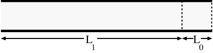
Figure 8: Disordered wire of length $L_{1}$ to which a segment of length $L_{0}$ is added. This scaling operation leads to a Brownian motion of the transmission eigenvalues determining the conductance. Taken from ref. [15]. Used with permission.

The resulting equation reads

$$\frac{\partial P}{\partial s}=DP$$ (20.1)

where $s$ is the wire length measured in units of the mean free path $l$: $s\equiv L/l$, and $D$ can be written in terms of the $\{\lambda_{i}\}$ as follows:

$$D=\frac{2}{\gamma}\sum_{i=1}^{N}\frac{\partial}{\partial\lambda_{i}}\lambda_{i}(1+\lambda_{i})J_{\beta}(\lambda)\frac{\partial}{\partial\lambda_{i}}J_{\beta}(\lambda)^{-1},$$ (20.2)

with $\gamma\equiv\beta N+2-\beta$. $\beta$ is the symmetry index of the ensemble of scattering matrices, in analogy with the well–known Wigner–Dyson classification, and $J_{\beta}(\lambda)\equiv J(\{\lambda_{i}\})$ is given by

$$J_{\beta}(\lambda)=\prod_{i<j}|\lambda_{j}-\lambda_{i}|^{\beta}$$ (20.3)

The solution of this equation was not at all immediate. What’s more, the appearance of $J_{\beta}(\{\lambda_{i}\})$ in the DMPK equation is due to the fact that the authors tried to mimick the Wigner–Dyson ensembles. However, this is quite misleading from the point of view of symmetric spaces, as the Wigner–Dyson ensembles have nothing to do with the transformation from the transfer matrix ensembles to the space of the $\{\lambda_{i}\}$. As we will see, the final solution of this equation, which is exact for $\beta=2$ and approximate for $\beta=1,\ 4$, relies on the relationship of transfer matrices with symmetric spaces of negative curvature.

The exact solution of the DMPK equation in the $\beta=2$ case was first obtained in a remarkable paper [39] by Beenakker and Rejaei. Here we review their derivation in a slightly different language, trying to stress the symmetric space origin of their result.

The starting point is a mapping of the coordinates $\lambda_{i}$ onto the radial coordinates $x_{i}$ on the symmetric space:

$$\lambda_{i}\equiv{\rm sinh}^{2}x_{i}$$ (20.4)

The DMPK equation can then be rewritten as

$$\frac{\partial P}{\partial s}=\frac{1}{2\gamma}\,J(x)\Delta_{B}^{\prime}J^{-1}(x)P$$ (20.5)

where

$$J(\{x_{i}\})=\prod_{i<j}|\sinh^{2}x_{i}-\sinh^{2}x_{j}|^{\beta}\prod_{k}|\sinh 2x_{k}|$$ (20.6)

is the Jacobian and $\Delta_{B}^{\prime}$ is the radial part of the Laplace–Beltrami operator on the underlying symmetric space! As a consequence, we can identify the differential equation with the equation for free diffusion on the symmetric space as a function of dimensionless ”time” $s=L/l$ where $l$ is the mean free path related to diffusion in the quantum wire.

At this point one can follow two roads. On the first one, which was the one followed by Beenakker and Rejaei, one maps the DMPK equation onto a Schrödinger equation in imaginary time. This requires the substitution

$$P(\{x_{i}\},s)=J^{\frac{1}{2}}(\{x_{i}\})\Psi(\{x_{i}\},s)$$ (20.7)

A straightforward calculation shows that the DMPK equation then takes the form

$$-\frac{\partial\Psi}{\partial s}=({\cal H}-U)\Psi$$ (20.8)

where $U$ is a constant and ${\cal H}$ is a Hamiltonian of the form

$${\cal H}=-\frac{1}{2\gamma}\sum_{i}\left(\frac{\partial^{2}}{\partial x_{i}^{2}}+{\rm sinh}^{-2}(2x_{i})\right)+\frac{\beta(\beta-2)}{2\gamma}\sum_{i<j}\frac{{\rm sinh}^{2}(2x_{i})+{\rm sinh}^{2}(2x_{j})}{({\rm cosh}(2x_{i})-{\rm cosh}(2x_{j}))^{2}}$$ (20.9)

At this point the main goal has already been reached: it is easy to see that if $\beta=2$ the equation decouples:

$${\cal H}_{0}=-\frac{1}{2\gamma}\frac{\partial^{2}}{\partial x^{2}}-\frac{1}{2\gamma\sinh^{2}2x}.$$ (20.10)

The resulting equation was solved in [39] using Greens functions.

The second approach to a solution of eq.(20.5) also relies on the underlying symmetric space structure. Again, the starting point is the identification of the DMPK operator $D$ and the radial part of the Laplace–Beltrami operator $\Delta^{\prime}_{B}$ on the underlying symmetric space:

$$\frac{\partial P}{\partial s}=DP=\frac{1}{2\gamma}\,BP$$ (20.11)

where $\Delta_{B}^{\prime}=J^{-1}BJ$.

As a consequence of this identification, if $\Phi_{k}(x)$ is an eigenfunction of $\Delta_{B}^{\prime}$ with eigenvalue $k^{2}$, then $J(x)\Phi_{k}(x)$ will be an eigenfunction of the DMPK operator with eigenvalue $k^{2}/(2\gamma)$. Then the properties of the eigenfunctions of the $\Delta_{B}^{\prime}$ operator, which are zonal spherical functions, can be used to derive the exact solution of the DMPK equation for $\beta=2$ ([40], see also [41]). This was done by Caselle. As the details of this calculation are quite technical, we will not review it here. The exact solution for the probability distribution is in both cases

$$P(\{x_{n}\},s) = C(s)\prod_{i<j}(\sinh^{2}x_{j}-\sinh^{2}x_{i})\prod_{k}(\sinh 2x_{k})$$

$$\mbox{}\times{\rm Det}\left[\int_{0}^{\infty}\!\!dk\,\exp\left(-\frac{k^{2}s}{4N}\right)\tanh\left(\frac{\pi k}{2}\right)k^{2m-1}\,{\rm P}_{\frac{1}{2}({\rm i}k-1)}(\cosh 2x_{n})\right]$$

where ${\rm P}_{\nu}(z)$ denotes the Legendre functions of the first kind. The second way of solving this equation constitutes a non–trivial consistency check on the solution obtained by Beenakker and Rejaei.

The power of the description in terms of symmetric spaces becomes evident in the $\beta=1$ and $\beta=4$ cases, in which the interaction between the eigenvalues does not vanish and the first approach discussed above does not apply. On the contrary, the description in terms of zonal spherical functions also holds in these two cases. Even though for $\beta\not=2$ one does not know the explicit form of the zonal spherical functions, one can use an asymptotic expansion due to Harish–Chandra to get asymptotic solutions. The asymptotic results derived by Caselle can be found in [42].

21 Relation to Calogero–Sutherland models

An important role in our analysis is played by the class of integrable models known as Calogero–Sutherland (CS) models, which turn out to be deeply related to the theory of symmetric spaces. These models describe $n$ particles in one dimension, identified by their coordinates $q^{1},...,q^{n}$ and interacting (at least in the simplest version of the models) through a pair potential $v(q^{i}-q^{j})$. The Hamiltonian of such a system is given by

$${\cal H}=\frac{1}{2}\sum_{i=1}^{n}p_{i}^{2}+\sum_{\alpha\in R^{+}}g_{\alpha}^{2}\,v(q^{\alpha})$$

$$p_{i}=-i\frac{\partial}{\partial q^{i}},\ \ \ \ q^{\alpha}=q\cdot\alpha=\sum_{i=1}^{n}q^{i}\alpha_{i}$$ (21.1)

where the coordinate $q$ is $q=(q^{1},...,q^{n})$, $p_{1},...,p_{n}$ are the particle momenta, and the particle mass is set to unity. In eq. (21) $R^{+}$ is the subsystem of positive roots of the root system $R=\{\alpha^{1},...,\alpha^{\nu}\}$ related to a specific simple Lie algebra or symmetric space, and $n$ is the dimension of the maximal abelian subalgebra ${\bf H_{0}}$. The components of the positive root $\alpha=\alpha^{k}\in R^{+}$ are $\alpha^{k}_{1},...,\alpha^{k}_{n}$. The number of positive roots is $\nu/2$, where $\nu$ is the total number of roots. In general, the coupling constants $g_{\alpha}$ are the same for equivalent roots, namely those that are connected with each other by transformations of the Weyl group $W$ of the root system.

Several realizations of the potential $v(q^{\alpha})$ have been studied in the literature (for detailed discussions see the review by Olshanetsky and Perelomov, ref. [9]). We will be concerned with the following types of potentials:

$$v_{I}(\xi) = \xi^{-2}$$

$$v_{II}(\xi) = {\rm sinh}^{-2}\xi$$

$$v_{III}(\xi) = {\rm sin}^{-2}\xi$$ (21.2)

Example: The CS model corresponding to a $C_{n}$ root lattice is

$${\cal H}=-\frac{1}{2}\sum_{i=1}^{n}\frac{\partial^{2}}{\partial(q^{i})^{2}}+\sum_{i}\frac{g_{l}^{2}}{\sinh^{2}(2q^{i})}+\sum_{i<j}\left(\frac{g_{o}^{2}}{\sinh^{2}(q^{i}-q^{j})}+\frac{g_{o}^{2}}{\sinh^{2}(q^{i}+q^{j})}\right)$$ (21.3)

We remind the reader that the $C_{n}$ root system consists of root vectors $\{\pm 2e_{i},\pm e_{i}\pm e_{j},i\neq j\}$. The arguments of the $\sinh$–function are $q^{\alpha}_{k}=q\cdot\alpha^{k}=(q^{1},...,q^{n})\cdot(e_{i}\pm e_{j})=q^{i}\pm q^{j}$ ($i<j$) where $\alpha^{k}$ is an ordinary positive root of the root lattice $R$, and $(q^{1},...,q^{n})\cdot(\pm 2e_{i})=\pm 2q^{i}$ for the long roots. Note the different coupling constants for the ordinary and long roots.

Under rather general conditions (see [9] for a detailed discussion) these models are completely integrable, in the sense that they possess $n$ commuting integrals of motion. As we will now see, the Calogero–Sutherland Hamiltonians can then be mapped onto the radial parts of the Laplace–Beltrami operators on the relevant symmetric spaces. The mapping is

$${\cal H}=J^{\frac{1}{2}}(q)\frac{1}{2}(\Delta_{B}^{\prime}\pm\rho^{2})J^{-\frac{1}{2}}(q)\ \ \ \ \ \ \ (+\ \ {\rm for\ \ II},\ \ -\ \ {\rm for\ \ III},\ \ \rho=0\ \ {\rm for\ \ I})$$ (21.4)

where $\rho$ is the vector defined in (18.25) and $J(q)$ is the Jacobian for transformation to radial coordinates on the SS:

$$\begin{array}[]{c}\\ J(q)\\ \\ \end{array}=\begin{array}[]{ll}\prod_{\alpha\in R^{+}}[\,q^{\alpha}\,]^{m_{\alpha}}&{\rm I}\\ \prod_{\alpha\in R^{+}}[\,{\rm sinh}(q^{\alpha})\,]^{m_{\alpha}}&{\rm II}\\ \prod_{\alpha\in R^{+}}[\,{\rm sin}(q^{\alpha})\,]^{m_{\alpha}}&{\rm III}\\ \end{array}$$ (21.5)

Olshanetsky and Perelomov proved that this happens if and only if the coupling constants $g_{\alpha}$ in ${\cal H}$ take the following root values

$$g_{\alpha}^{2}=\frac{m_{\alpha}(m_{\alpha}+2m_{2\alpha}-2)|\alpha|^{2}}{8}$$ (21.6)

where $m_{\alpha}$ is the multiplicity of the root $\alpha$ and $|\alpha|$ is its length.

A number of results can be obtained for the corresponding quantum systems merely by using the theory of symmetric spaces. Due to equation (21.4), once we know the zonal spherical functions, we can solve the Schrödinger equation. A detailed collection of results pertaining to spectra, wave functions, and integral representations of wave functions can be found in the original article [9].

The equation (20.9) in the solution of the DMPK equation discussed in the previous section can be recast in a slightly different form, thus completing the chain of identifications

DMPK equation — symmetric space — Calogero–Sutherland model

By using simple identities for hyperbolic functions, the Hamiltonian in (20.9) becomes [42]

$$\gamma{\cal H}=\sum_{i}\left(-\frac{1}{2}\frac{\partial^{2}}{\partial x_{i}^{2}}+\frac{g_{l}^{2}}{{\rm sinh}^{2}(2x_{i})}\right)+\sum_{i<j}\left(\frac{g_{o}^{2}}{{\rm sinh}^{2}(x_{i}-x_{j})}+\frac{g_{o}^{2}}{{\rm sinh}^{2}(x_{i}+x_{j})}\right)+c$$ (21.7)

where $g_{l}^{2}\equiv-1/2$, $g_{o}^{2}\equiv\beta(\beta-2)/4$ and $c$ is an irrelevant constant. This Hamiltonian, apart from an overall factor $1/\gamma$ and the constant $c$, exactly coincides with the Calogero–Sutherland Hamiltonian (21.3) corresponding to a root lattice $R=\{\pm 2x_{i},\pm x_{i}\pm x_{j},i\neq j\}$ of type $C_{n}$ with root multiplicities $m_{o}=\beta$, $m_{l}=1$. The values of the coupling constants $g_{o}$, $g_{l}$ are exactly the root values given in eq. (21.6) for which the transformation from ${\cal H}$ into $\Delta_{B}^{\prime}$ is possible.

22 Concluding remarks

In these lectures we have given an elementary introduction to random matrix theory, as well as discussed some basic concepts in the theory of symmetric spaces. The scope of these discussions were to show, through numerous examples, that hermitean random matrix ensembles and the symmetric coset spaces based on simple Lie groups and classified by Cartan, are the same mathematical objects. By making this identification, new results can be obtained in random matrix theory by applying what is known in mathematics about such manifolds. We gave a few examples of this in the last lecture.

In the first lecture we discussed a number of systems that are successfully described by random matrix theories. (Due to the limited expertise of the author, only some major applications in physics were discussed, however, there are also applications for instance in mathematics and biology.) We saw that random matrix theory gives a statistical description of complex eigenvalue spectra of quantum operators in chaotic or many–body systems. By taking the double scaling limit in which the spectrum becomes dense and the eigenvalues are simultaneously rescaled on the scale of the average level spacing, one can separate out the universal part of the spectral behavior from the system–dependent one. We briefly discussed some typical spectral observables obtainable from the correlation functions. A large number of systems (some of which were discussed in the introduction) exhibit the generic spectral features arising in random matrix theory.

One such system is represented by quarks in a random gauge field background. We illustrated this by showing a few graphs of computer simulations of QCD–like gauge theories on a space–time lattice. In these the spectrum of the Dirac operator was studied and compared to analytical predictions from random matrix theory. Of course, there is a wealth of experimental and numerical results also on the spectra of nuclei, atoms, molecules, elastomechanical systems, microwave cavities, mesoscopic systems, etc., that we have not even mentioned and that could be given as examples of the type of spectral behavior that is predicted by random matrix theory. It is important to note that RMT behavior in spectra can also be partial, depending on circumstances not always fully understood (see [2] for a discussion).

The typical eigenvalue repulsion in chaotic systems described by RMT can be traced to the geometrical properties of the corresponding symmetric space manifold. In particular we discussed how curvature, type of roots, and root multiplicities of the restricted root lattice on the symmetric manifold determine the exact form of these correlations. This follows from the general theory of coordinate systems on symmetric spaces and from the identification of the radial coordinates on the symmetric space with the set of random matrix eigenvalues. We made a number of further identifications between matrix ensembles and symmetric spaces and summarized the results in Table 4.

We also explained how symmetric spaces corresponding to compact symmetric subgroups are classified. All possible involutive automorphisms of the compact real form of an algebra leads, in a natural way, to a classification based on root lattices. This defines the universality classes of the corresponding random matrix ensembles, and leads to a new scheme of classification dictated by the strict properties of root systems belonging to simple complex Lie algebras.

The differential equation for quantum wires called the DMPK equation describes the evolution with increasing wire length of the joint probability distribution of a set of parameters simply related to the transmission eigenvalues. In our discussion we concluded that it essentially corresponds to the equation for free diffusion on the symmetric space, and we discussed its solution in terms of zonal spherical functions for all three values of the Dyson index. The zonal spherical functions are known in the theory of symmetric spaces, where they play the role of eigenfunctions for the radial part of the Laplace–Beltrami operator on the symmetric manifold.

Lastly, we discussed work by Olshanetsky and Perelomov on the integrability of a class of one–dimensional Calogero–Sutherland models. Such models become integrable at certain “root values” of the coupling constants, and the integrals of motion are then given by the Casimir operators related to the Lie algebra or symmetric space underlying the model. This leads to a set of exact results concerning spectra and wave functions of quantum systems.

It is certainly of interest to further investigate the possibility of applying known results on symmetric spaces to the corresponding ensembles of random matrices. An important research direction might be trying to fit also non–hermitean ensembles into a similar setting. This would bring us outside Cartan’s scheme. In spite of the recent activity in the field of non–hermitean random matrix ensembles, the author is not aware of any research effort in this direction. There are also various types of extensions of Calogero–Sutherland models that could be explored in this spirit.

References

- [1] M. Caselle and U. Magnea, Phys. Rep. 394 (2004) 41-156, cond-mat/0304363
- [2] T. Guhr, A. Müller–Groeling and H. A. Weidenmüller, Phys. Rep. 299 (1998) 189, cond-mat/9707301
- [3] F. J. Dyson, J. Math. Phys. 3 (1962) 140, 157, 166, 1191, 1199
- [4] F. Dyson, Comm. Math. Phys. 19 (1970) 235
- [5] A. Hüffmann, J. Phys. A23 (1990) 5733
- [6] S. Helgason, Differential Geometry, Lie Groups and Symmetric Spaces (Academic, New York 1978) ISBN: 0-12-338460-5
- [7] S. Helgason, Groups and geometric analysis: Integral geometry, invariant differential operators, and spherical functions (Academic, New York 1984) ISBN: 0-12-338301-3
- [8] R. Gilmore, Lie groups, Lie algebras, and some of their applications (John Wiley & Sons, New York 1974) ISBN: 0-471-30179-5
- [9] M. A. Olshanetsky and A. M. Perelomov, Phys. Rep. 94 (1983) 313
- [10] P. Heinzner, A. Huckleberry and M. R. Zirnbauer, math-ph/0411040
- [11] G. Akemann, Phys.Lett. B547 (2002) 100, hep-th/0206086; G. Akemann and G. Vernizzi, Nucl. Phys. B660 (2003) 532, hep-th/0212051
- [12] J. Ambjorn, Lectures presented at the 1994 Les Houches Summer School “Fluctuating Geometries in Statistical Mechanics and Field Theory”, hep-th/9411179
- [13] E. P. Wigner, Ann. Math. 67 (1958) 325
- [14] O. Bohigas, R.U. Haq and A. Pandey, “Nuclear data for science and technology”, K.H. Böhhoff (ed.), Reidel, Dordrecht (1983).
- [15] C. W. J. Beenakker, Rev. Mod. Phys. 69 (1997) 731, cond-mat/9612179
- [16] Reprinted with permission from C.M. Marcus, A.J. Rimberg, R.M. Westervelt, P.F. Hopkins and A.C. Gossard, Phys. Rev. Lett. 69 (1992) 506,121212Readers may view, browse, and/or download material for temporary copying purposes only, provided these uses are for noncommercial personal purposes. Except as provided by law, this material may not be further reproduced, distributed, transmitted, modified, adapted, performed, displayed, published, or sold in whole or part, without prior written permission from the publisher. http://link.aps.org/abstract/PRL/v69/p506
- [17] A. Altland and M. R. Zirnbauer, Phys. Rev. Lett. 76 (1996) 3420, cond-mat/9508026; A. Altland and M. R. Zirnbauer, Phys. Rev. B55 (1997) 1142, cond-mat/9602137
- [18] K. B. Efetov, Zh. Eksp. Teor. Fiz. 83 (1982) 833 [Sov. Phys. JETP 56, 467]; K. B. Efetov, Adv. Phys. 32 (1983) 53
- [19] J.J.M. Verbaarschot, “The Supersymmetric Method in Random Matrix Theory and Applications to QCD”, Lectures given at the 2004 ELAF Summer School in Mexico City, hep-th/0410211
- [20] See for example E.V. Shuryak, J.J.M. Verbaarschot, Nucl. Phys. A560 (1993) 306, hep-th/9212088; J.J.M. Verbaarschot, I. Zahed, Phys. Rev. Lett. 70 (1993) 3852 hep-th/9303012; J. Verbaarschot, Phys. Rev. Lett. 72 (1994) 2531 hep-th/9401059
- [21] M.A. Halasz, J.J.M. Verbaarschot, Phys. Rev. D52 (1995) 2563 hep-th/9502096; D. Toublan, J.J.M. Verbaarschot, Nucl. Phys. B560 (1999) 259, hep-th/9904199; U. Magnea, Phys.Rev. D61 (2000) 056005, hep-th/9907096; U. Magnea, Phys.Rev. D62 (2000) 016005, hep-th/9912207
- [22] Jac Verbaarschot, “QCD, chiral random matrix theory and integrability”, hep-th/0502029
- [23] See for instance: B. A. Berg, H. Markum, R. Pullirsch, T. Wettig, Phys. Rev. D63 (2001) 014504, hep-lat/0007009 and references therein.
- [24] J. J. M. Verbaarschot, The infrared limit of the QCD Dirac spectrum and applications of chiral random matrix theory to QCD (lectures given at the APCTP-RCNP Joint International School on Physics of Hadrons and QCD (Osaka, 1998) and the 1998 YITP-Workshop on QCD and Hadron Physics (Kyoto, 1998)), hep-ph/9902394; J. J. M. Verbaarschot and T. Wettig, Ann. Rev. Nucl. Part. Sci. 50 (2000) 343, hep-ph/0003017
- [25] G. Akemann, J.C. Osborn, K. Splittorff, J.J.M. Verbaarschot, hep-th/0411030
- [26] M. L. Mehta, Random matrices (revised and enlarged edition; Academic press, San Diego 1991) ISBN: 0-12-488051-7
- [27] M. E. Berbenni–Bitsch, S. Meyer, A. Schäfer, J.J.M. Verbaarschot and T. Wettig, Phys. Rev. Lett. 80 (1998) 1146, hep-lat/9704018
- [28] Reprinted with permission from C. Ellegaard, T. Guhr, K. Lindemann, J. Nygård and M. Oxborrow, Phys. Rev. Lett. 77 (1996) 4918 (see footnote in ref. [16]), http://link.aps.org/abstract/PRL/v77/p4918
- [29] J. Verbaarschot, Nucl. Phys. B (Proc. Suppl.) 53 (1997) 88
- [30] H. Georgi, Lie algebras in particle physics (Benjamin/Cummings, Reading, Mass., 1982) ISBN: 0-8053-3153-0
- [31] O. Loos, Symmetric spaces, vol. II (W.A. Benjamin Inc., New York 1969)
- [32] D. H. Sattinger, O. L. Weaver: Lie groups and algebras with applications to physics, geometry and mechanics (Springer-Verlag, New York 1986) ISBN: 3540962409
- [33] R. Landauer, Philos. Mag. 21 (1970) 863
- [34] D.S. Fisher and P.A. Lee, Phys. Rev. B23 (1981) 6851
- [35] M. Büttiker, Y. Imry, R. Landauer, S. Pinhas, Phys. Rev. B31 (1985) 6207
- [36] P. A. Mello, P. Pereyra, N. Kumar, Ann. Phys. 181 (1988) 290
- [37] T. Nagao and P. J. Forrester, Nucl. Phys. B435 (1995) 401
- [38] O. N. Dorokhov, Pis’ma Zh. Eksp. Teor. Fiz. 36 (1982) 259; JETP Lett. 36 (1982) 318
- [39] C. W. J. Beenakker and B. Rejaei, Phys. Rev. Lett. 71 (1993) 3689; Phys. Rev. B49 (1994) 7499, cond-mat/9310066
- [40] P. W. Brouwer, C. Mudry, B. D. Simons, A. Altland, Phys. Rev. Lett. 81 (1998) 862, cond-mat/9807189
- [41] P. W. Brouwer, A. Furusaki, I. A. Gruzberg, C. Mudry, Phys. Rev. Lett. 85 (2000) 1064; cond-mat/0002016
- [42] M. Caselle, Phys. Rev. Lett. 74 (1995) 2776, cond-mat/9410097