Branched quantum wave guides with Dirichlet boundary conditions: the decoupling case

Abstract.

We consider a family of open sets ${M_{\varepsilon}}$ which shrinks with respect to an appropriate parameter $\varepsilon$ to a graph. Under the additional assumption that the vertex neighbourhoods are small we show that the appropriately shifted Dirichlet spectrum of ${M_{\varepsilon}}$ converges to the spectrum of the (differential) Laplacian on the graph with Dirichlet boundary conditions at the vertices, i.e., a graph operator without coupling between different edges. The smallness is expressed by a lower bound on the first eigenvalue of a mixed eigenvalue problem on the vertex neighbourhood. The lower bound is given by the first transversal mode of the edge neighbourhood. We also allow curved edges and show that all bounded eigenvalues converge to the spectrum of a Laplacian acting on the edge with an additional potential coming from the curvature.

1. Introduction

Graph models of quantum systems can often be used to describe in a simple way some important aspects of the behaviour of a quantum system. Although such models are simple enough to be solvable (because they are essentially $1$-dimensional) they still have enough structure to model real systems. Ruedenberg and Scherr [RuS53] used this idea to calculate spectra of aromatic carbohydrate molecules. Nowadays the rapid technical progress allows to fabricate structures of electronic devices where quantum effects play a dominant role. Graph models like quantum graphs (also called metric graphs) can often be viewed as a good approximation of such structures. From the mathematical point of view these models were analysed first thoroughly in [EŠ89] , for recent developments, bibliography and further applications see [DE95], [KoS99], [Ku02] or [Ku04]; note that [KaP88] also calculated the eigenvalue asymptotic of a tubular $\varepsilon$-neighbourhood of a curve.

A quantum (or metric) graph is a graph where we associate a length to each edge. A natural operator acting on such graphs is given by a self-adjoint extension of $-d^{2}/dx^{2}$ on each edge. We will call such a self-adjoint extension a Laplacian on the (quantum) graph. Note that the Laplacian on a discrete graph is a difference operator on $\ell_{2}({K})$ rather than a differential operator acting in $\bigoplus_{j}L_{2}({e_{j}})$. Here, $K$ labels the vertices and $J$ the edges $e_{j}$, $j\in J$, of the graph. A detailed overview on this wide field can be found in [Ku04] or [KoS99].

A natural question is in what mathematical sense a quantum graph $M_{0}$ can be approximated by a more smooth space ${M_{\varepsilon}}$. One is interested what Laplacians on $M_{0}$ occur as limit operators from operators on ${M_{\varepsilon}}$. More significantly, ${M_{\varepsilon}}$ could be the $\varepsilon$-neighbourhood of an embedded graph $M_{0}\subset\mathbb{R}^{n}$ or a manifold shrinking to $M_{0}$ as $\varepsilon\to 0$. We call such approximating spaces branched quantum wave guides. Recently, spectral convergence in the case of a bounded open set ${M_{\varepsilon}}$ with Neumann boundary condition has been established in [RSc01], [KuZ01] and [KuZ03]; for an approximation by manifolds see [EP04]. All these examples have in common, that the lowest eigenmode of the transversal direction is $0$ with constant eigenfunction. In this case, the limit operator is the Laplacian on the graph with Kirchhoff boundary conditions, i.e., a function $f$ in the domain of the Kirchhoff Laplacian is continuous at each vertex and satisfies

$$\sum_{j\in J_{k}}f_{j}^{\prime}(v_{k})=0,\qquad k\in K.$$ (1.1)

In addition, the spectral convergence holds independently of a given embedding of the graph. In particular, the convergence is independent of the curvature of the embedded edges.

The case of an approximation by Dirichlet Laplacians on an open set ${M_{\varepsilon}}$ was first treated heuristically in [RuS53]. This case is harder to analyse since the first transversal eigenvalue equals $\lambda^{\mathrm{D}}_{1}({F_{\varepsilon}})=\lambda_{1}/\varepsilon^{2}$ ($\lambda_{1}>0$), i.e., it is of the order $\varepsilon^{-2}$ if $\varepsilon$ denotes the radius of the cross section $F_{\varepsilon}=(-\varepsilon,\varepsilon)$ of the approximating set ${M_{\varepsilon}}$. A rescaling is necessary, and first order terms of the metric $g_{\varepsilon}$ (cf. (4.3)) like the curvature become important. In particular, the curvature of the (embedded) edge enters in the limit operator as an additional potential.

Main result

Assume that $M_{0}\subset\mathbb{R}^{2}$ is a finite graph. Our aim in this note is to show the spectral convergence of the Dirichlet Laplacian on an approximating open set ${M_{\varepsilon}}\supset M_{0}$. We suppose that ${M_{\varepsilon}}$ can be decomposed into neighbourhoods ${U_{\varepsilon,j}}$ of the edges $e_{j}$ and into neighbourhoods ${V_{\varepsilon,k}}$ of the vertices $v_{k}$ of $M_{0}$ (cf. Figure 1). We assume that ${V_{\varepsilon,k}}$ is $\varepsilon$-homothetic to a fixed set ${V_{k}}$.

Figure 1. Decomposition of the graph neighbourhood ${M_{\varepsilon}}$ (grey) of the graph $M_{0}$ into edge and vertex neighbourhoods ${U_{\varepsilon,j}}$ and ${V_{\varepsilon,k}}$.

The precise definition will be given in Section 2 and 4. Our basic assumption is that the vertex neighbourhoods ${V_{\varepsilon,k}}$ are small,

Figure 2. The scaled vertex neighbourhood ${V_{k}}$ with the boundary part $\partial_{0}{V_{k}}$ coming from the original boundary and the boundary part $\partial_{j}{V_{k}}$ where the edge $e_{j}$ emanates.

i.e., that

$$\lambda^{{\mathrm{D}}{\mathrm{N}}}_{1}({{V_{k}}})>\lambda^{\mathrm{D}}_{1}({F})=\lambda_{1}$$ (1.2)

where $\lambda^{{\mathrm{D}}{\mathrm{N}}}_{1}({{V_{k}}})$ is the lowest eigenvalue of the Laplacian $\Delta^{{\mathrm{D}}{\mathrm{N}}}_{{{V_{k}}}}$ of ${V_{k}}$ with Dirichlet boundary conditions on $\partial_{0}{V_{k}}$ (i.e., on the boundary induced from the original boundary of ${M_{\varepsilon}}$) and Neumann boundary conditions on $\partial_{j}{V_{k}}$, $j\in J_{k}$, (i.e., on the parts where the adjacent edge neighbourhoods labeled by $j\in J_{k}$ emanate, cf. Figure 2). Furthermore, $F=(-1,1)$ and therefore $\lambda_{1}=\pi^{2}/4$. We comment on this condition in Section 5.

Our main result is

Theorem 1.1.

Suppose that ${M_{\varepsilon}}$ is an open neighbourhood of a finite graph $M_{0}\subset\mathbb{R}^{2}$ satisfying the smallness assumption (1.2) on each vertex neighbourhood. Denote by $\lambda_{k}({\varepsilon})$ the $k$-th eigenvalue of the Dirichlet-Laplacian $\Delta^{\mathrm{D}}_{{{M_{\varepsilon}}}}\geq 0$ (counted with respect to multiplicity). Then

$$\lambda_{k}({\varepsilon})-\frac{\lambda_{1}}{\varepsilon^{2}}\to\lambda_{k}({0}),\qquad\varepsilon\to 0$$ (1.3)

where $\lambda_{k}({0})$ denotes the $k$-th eigenvalue of

$$\bigoplus_{j\in J}(\Delta^{\mathrm{D}}_{{I_{j}}}-\kappa_{j}^{2}/4)$$

with $\Delta^{\mathrm{D}}_{{e_{j}}}=-d^{2}/dx_{j}^{2}$ being the Dirichlet Laplacian on the edge $e_{j}\cong I_{j}=(0,\ell_{j})$ and $\kappa_{j}$ being the curvature of the embedded edge $e_{j}\subset\mathbb{R}^{2}$ (cf. (4.2)).

Note that the smallness assumption at the junctions ${V_{\varepsilon,k}}$ implies that the limit operator decouples, i.e., the limit operator is the direct sum of operators acting on a single edge. In the case of the Neumann Laplacian on ${M_{\varepsilon}}$ decoupling occurs if the area of the edge neighbourhood decays faster than the area of the vertex neighbourhood; e.g., if the latter scales in each direction of the order $\varepsilon^{\alpha}$ with $0\leq\alpha<1/2$; the vertex neighbourhoods are large obstacles seen from the edge neighbourhoods (cf. [KuZ03] or [EP04]). In the case of Dirichlet boundary conditions, in contrast, decoupling already occurs when the vertex neighbourhoods scale with $\varepsilon$, i.e., even when the edge neighbourhood volume (which is of order $\varepsilon$) decays slower than the vertex neighbourhood volume (of order $\varepsilon^{2}$).

We also show in Section 5 that the usual $\varepsilon$-neighbourhood ${M_{\varepsilon}}:=\{\,z\in\mathbb{R}^{2}\,|\,d(z,M_{0})<\varepsilon\,\}$ does not satisfy our hypothesis since the leading order of the lowest eigenvalue is at most $\mu/\varepsilon^{2}$ with $\mu<\lambda_{1}$. Therefore, $\Delta^{\mathrm{D}}_{{{M_{\varepsilon}}}}-\lambda_{1}/\varepsilon^{2}$ has a negative eigenvalue tending to $-\infty$ (cf. also Lemma 2.1) and the conclusion of Theorem 1.1 fails. In particular, there is no limit operator on the graph (using the simple shift $\lambda\to\lambda-\lambda_{1}/\varepsilon^{2}$), and the suggestion in [RuS53], that the limit operator is the Kirchhoff Laplacian on $M_{0}$, is false (cf. also [Ku02, Sec. 2.1 and 3.2]). Note that Ruedenberg and Scherr implicitly assumed that the lowest eigenfunction does not concentrate around the vertex which is the case as we will see in the last section.

The spectral convergence of a single curved quantum wave guide has already been shown in [DE95] and [KaP88] using perturbation methods. Our proof only uses variational methods and is a simple adaption of [EP04], [KuZ01, KuZ03] or [RSc01], where one compares Rayleigh quotients.

The paper is structured as follows: In the next section we define the required spaces and operators in the case of straight edges. Section 3 is devoted to the proof of Theorem 1.1 in this case. In Section 4 we provide the necessary changes in order to prove the result with curved edges. Section 5 contains some explantation on the smallness condition (1.2), and examples where this condition holds or fails.

2. Preliminaries

In this section we define the limit space and the approximating space together with the associated operators. We first consider straight edges without curvature, i.e., $\kappa_{j}=0$. In Section 4 we also allow curved edges.

Definition of the limit space

Let $M_{0}$ be a finite connected graph with (metric) edges $e_{j}$, $j\in J$ ($e_{j}$ isometric to an open interval $I_{j}=(0,\ell_{j})$) and vertices $v_{k}$, $k\in K$. We denote the set of all $j\in J$ such that $e_{j}$ emanates from the vertex $v_{k}$ by $J_{k}$. The Hilbert space associated to such a graph is

$$\mathcal{H}:=L_{2}({{M_{0}}})=\bigoplus_{j\in J}L_{2}({{I_{j}}})$$

which consists of all functions $f$ with finite norm

$$\|{f}\|^{2}_{0}=\|{f}\|^{2}_{{M_{0}}}=\sum_{j\in J}\|{f_{j}}\|^{2}_{{I_{j}}}=\sum_{j\in J}\int_{{I_{j}}}|f_{j}(x)|^{2}\,dx.$$

Definition of the limit operator

We define the limit operator $Q_{0}$ via the quadratic form

$$q_{0}(f):=\sum_{j\in J}\|{f^{\prime}_{j}}\|^{2}_{{I_{j}}}=\sum_{j\in J}\int_{{I_{j}}}|f^{\prime}_{j}(x)|^{2}dx$$

for functions $f\in C_{\mathrm{c}}^{\infty}({{M_{0}}})=\bigoplus_{j}C_{\mathrm{c}}^{\infty}({{I_{j}}})$ (with compact support). The form closure of $q_{0}$ (also denoted by $q_{0}$) is the extension of $q_{0}$ to the closure of the space of all such functions in the norm

$$\|{f}\|^{2}_{0,1}:=\|{f}\|^{2}_{0}+q_{0}(f)$$

(see [K66, Chapter VI], [RS80] or [Da96] for details on quadratic forms). Note that

$$\operatorname{dom}q_{0}=\bigoplus_{j\in J}{{\makebox[7.50002pt]{\raisebox{6.83331pt}{\hskip 1.93747pt$\scriptscriptstyle\circ$}}\makebox[0.0pt][r]{${\mathcal{H}}$}}{}^{1}({{I_{j}}})}.$$

Remember that ${{\makebox[7.50002pt]{\raisebox{6.83331pt}{\hskip 1.93747pt$\scriptscriptstyle\circ$}}\makebox[0.0pt][r]{${\mathcal{H}}$}}{}^{1}({I})}$ is the closure of $C_{\mathrm{c}}^{\infty}({I})$ w.r.t. the norm $(\|{f}\|^{2}+\|{f^{\prime}}\|^{2})^{1/2}$. The associated self-adjoint, non-negative operator $Q_{0}$ is given by

$$Q_{0}=\bigoplus_{j\in J}\Delta^{\mathrm{D}}_{{{I_{j}}}}$$ (2.1)

where $\Delta^{\mathrm{D}}_{{{I_{j}}}}\geq 0$ denotes the self-adjoint operator $-d^{2}/dx^{2}$ on ${I_{j}}$ with Dirichlet boundary conditions. The spectrum of $Q_{0}$ is purely discrete and will be denoted by $\lambda_{k}({0})$, written in ascending order and repeated according to multiplicity.

Definition of the approximating space

We now describe the family of open sets $({M_{\varepsilon}})_{\varepsilon}$, $0<\varepsilon\leq\varepsilon_{0}$, approximating the graph $M_{0}$ as $\varepsilon\to 0$. For convenience only, suppose that $M_{0}$ is embedded in $\mathbb{R}^{2}$ (an abstract definition of ${M_{\varepsilon}}$ in the general case will be given soon). Assume that we can decompose ${M_{\varepsilon}}$ into open sets ${U_{\varepsilon,j}}$ containing those points $x\in e_{j}$ with $d(x,\partial e_{j})>a_{j}\varepsilon/2$ for some real number $a_{j}<1/\varepsilon_{0}$ and ${V_{\varepsilon,k}}\ni v_{k}$ such that the union of their closures equals $\overline{M_{\varepsilon}}$. Here, the edge neighbourhood ${U_{\varepsilon,j}}$ is isometric to $I_{\varepsilon,j}\times F_{\varepsilon}$ (both equipped with the Euclidean metric) where $I_{\varepsilon,j}:=(0,(1-a_{j}\varepsilon)\ell_{j})$ and $F_{\varepsilon}=(-\varepsilon,\varepsilon)$ is the scaled cross section. Furthermore, we assume that the vertex neighbourhood ${V_{\varepsilon,k}}$ is $\varepsilon$-homothetic to a fixed open set ${V_{k}}$. Using a simple coordinate transform we have therefore the isometries

$$({U_{\varepsilon,j}},g_{\mathrm{eucl}})\cong({I_{j}}\times F,{g_{\varepsilon}})\qquad\text{and}\qquad({V_{\varepsilon,k}},g_{\mathrm{eucl}})\cong({V_{k}},{g_{\varepsilon}})$$ (2.2)

where

$${g_{\varepsilon}}=(1-\varepsilon a_{j})^{2}dx^{2}+\varepsilon^{2}dy^{2}\qquad\text{and}\qquad{g_{\varepsilon}}=\varepsilon^{2}g$$ (2.3)

are the metrics on the edge resp. vertex neighbourhood. Here, $F=(-1,1)$ and $g$ is the Euclidean metric on ${V_{k}}$. In the sequel we use this change of coordinate transform without mentioning. Note that the slightly shortened edge neighbourhood is necessary in order to have an embedding for the edge and the vertex neighbourhood.

Although we are mainly interested in the embedded situation as described above, we prefer the following abstract setting in order to keep the notation of [EP04] and recognise the important geometric objects (not depending on any embedding). For each $j\in J$ we let ${U_{\varepsilon,j}}$ be the Riemannian manifold $({I_{j}}\times F,{g_{\varepsilon}})$ where ${g_{\varepsilon}}$ is given as in (2.3). Here $F$ is the interior of a compact, connected $m$-dimensional manifold ($m\geq 1$) with metric denoted by $dy^{2}$ having purely discrete Dirichlet spectrum with first eigenvalue $\lambda_{1}>0$.

Furthermore, we denote by ${V_{\varepsilon,k}}$ the Riemannian manifold $({V_{k}},{g_{\varepsilon}})$ with ${g_{\varepsilon}}=\varepsilon^{2}g$ where $g$ is a metric on ${V_{k}}$. We assume that

$$\partial{V_{k}}=\partial_{0}{V_{k}}\cup\bigcup_{j\in J_{k}}\partial_{j}{V_{k}},$$ (2.4)

i.e., the boundary of ${V_{k}}$ has as many boundary parts $\partial_{j}{V_{k}}$ isometric to $F$ as edges emanate from $v_{k}$ and $\partial_{0}{V_{k}}$ is the closure of $\partial{V_{k}}\setminus\bigcup_{j}\partial_{j}{V_{k}}$ (cf. Figure 2). Furthermore, we assume that the metric on ${V_{k}}$ has product structure $g=dx^{2}+dy^{2}$ near $\partial_{j}{V_{k}}$.

We can define an abstract manifold ${M_{\varepsilon}}$ by identifying the appropriate boundary parts according to the graph $M_{0}$. Note that a smooth structure on ${M_{\varepsilon}}$ and also a smooth metric $g_{\varepsilon}$ of the form (2.3) in the respective charts exist since ${M_{\varepsilon}}$ is diffeomorphic to a product $(0,1)\times F$ in a neighbourhood of each $\partial_{j}{V_{k}}$ on both sides of $\partial_{j}{V_{k}}$, i.e., on ${V_{k}}$ and ${U_{j}}$. Strictly speaking we should introduce another chart for each $j\in J_{k}$ and $k\in K$ covering $\partial_{j}{V_{k}}$ in order to define the smooth structure properly. But since we only use integrals over ${M_{\varepsilon}}$, a cover up to sets of measure $0$ is enough. The resulting manifold has dimension $d=m+1$. Note that ${M_{\varepsilon}}$ need not to be embedded in any space, but the embedded case described above is also covered by this setting.

The associated Hilbert space is

$$L_{2}({{M_{\varepsilon}}})=\bigoplus_{j\in J}L_{2}({{U_{\varepsilon,j}}})\oplus\bigoplus_{k\in K}L_{2}({{V_{\varepsilon,k}}})$$

which consists of all functions $u$ with finite norm

$$\|{u}\|^{2}_{\varepsilon}=\|{u}\|^{2}_{{M_{\varepsilon}}}=\sum_{j\in J}\|{u}\|^{2}_{{U_{\varepsilon,j}}}+\sum_{k\in K}\|{u}\|^{2}_{{V_{\varepsilon,k}}}\\ =\sum_{j\in J}\int_{{I_{j}}\times F}|u|^{2}(1-a_{j}\varepsilon)\varepsilon^{m}\,dx\,dy+\sum_{k\in K}\int_{{V_{k}}}|u|^{2}\varepsilon^{d}dz$$

where $dy$ and $dz$ represent the natural measures on $F$ and ${V_{k}}$, respectively.

Definition of the operator on the manifold

The operator on the thickened space we are considering will be the Dirichlet Laplacian on ${M_{\varepsilon}}$, i.e., $H_{\varepsilon}=\Delta^{\mathrm{D}}_{{{M_{\varepsilon}}}}\geq 0$. The corresponding quadratic form $h_{\varepsilon}$ is given by

$$h_{\varepsilon}(u)=\sum_{j\in J}\|{du}\|^{2}_{{U_{\varepsilon,j}}}+\sum_{k\in K}\|{du}\|^{2}_{{V_{\varepsilon,k}}}\\ =\sum_{j\in J}\int_{{I_{j}}\times F}\Bigl{[}\frac{1}{(1-a_{j}\varepsilon)^{2}}|\partial_{x}u|^{2}+\frac{1}{\varepsilon^{2}}|d_{y}u|^{2}\Bigr{]}(1-a_{j}\varepsilon)\varepsilon^{m}\,dx\,dy+\sum_{k\in K}\int_{{V_{k}}}|du|^{2}\varepsilon^{d-2}dz$$

for functions $u\in\operatorname{dom}h_{\varepsilon}={{\makebox[7.50002pt]{\raisebox{6.83331pt}{\hskip 1.93747pt$\scriptscriptstyle\circ$}}\makebox[0.0pt][r]{${\mathcal{H}}$}}{}^{1}({{M_{\varepsilon}}})}$ where ${{\makebox[7.50002pt]{\raisebox{6.83331pt}{\hskip 1.93747pt$\scriptscriptstyle\circ$}}\makebox[0.0pt][r]{${\mathcal{H}}$}}{}^{1}({{M_{\varepsilon}}})}$ is the closure of $C_{\mathrm{c}}^{\infty}({{M_{\varepsilon}}})$ in the norm $(\|{u}\|^{2}+h_{\varepsilon}(u))^{1/2}$. Here, $|d_{y}u|^{2}$ and $|du|^{2}$ are evaluated in the ($\varepsilon$-independent) metric of the exterior derivative of $u(x,\cdot)$ and $u$ on $T^{*}F$ and $T^{*}{V_{k}}$, respectively.

The spectrum of $H_{\varepsilon}$ is again purely discrete (since $\overline{M_{\varepsilon}}$ is compact) and will be denoted by $\lambda_{k}({\varepsilon})$, written in ascending order and repeated according to multiplicity. By the the min-max principle we have

$$\lambda_{k}({\varepsilon})=\inf_{L_{k}}\sup_{u\in L_{k}\setminus\{0\}}\frac{h_{\varepsilon}(u)}{\|{u}\|^{2}_{\varepsilon}},$$ (2.5)

where the infimum is taken over all $k$-dimensional subspaces $L_{k}$ of $\operatorname{dom}h_{\varepsilon}$, cf. e.g. [Da96].

We denote by $F_{\varepsilon}$ the manifold $F$ with metric $\varepsilon^{2}dy^{2}$ and the first Dirichlet eigenvalue of $F$ by $\lambda_{1}=\lambda^{\mathrm{D}}_{1}({F})>0$. Since the lowest eigenvalue of $F_{\varepsilon}$ is $\lambda_{1}/\varepsilon^{2}$, we need a rescaling of the operator $H_{\varepsilon}$ in order to expect convergence to an $\varepsilon$-independent limit operator. Therefore we set

$$Q_{\varepsilon}:=H_{\varepsilon}-\frac{\lambda_{1}}{\varepsilon^{2}}$$ (2.6)

and denote by $q_{\varepsilon}$ the associated quadratic form.

We first note that the operator $Q_{\varepsilon}$ is positive:

Lemma 2.1.

Suppose the smallness condition (1.2) is fulfilled, then $Q_{\varepsilon}\geq 0$.

Proof.

For $u\in\operatorname{dom}q_{\varepsilon}=\operatorname{dom}h_{\varepsilon}$ we have

$$q_{\varepsilon}(u)=\sum_{j\in J}\int_{{I_{j}}}\Bigl{[}\frac{1}{(1-a_{j}\varepsilon)^{2}}\|{\partial_{x}u(x,\cdot)}\|^{2}_{F}\\ +\frac{1}{\varepsilon^{2}}\bigl{(}\|{d_{y}u(x,\cdot)}\|^{2}_{F}-\lambda_{1}\|{u(x,\cdot)}\|^{2}_{F}\bigr{)}\Bigr{]}(1-a_{j}\varepsilon)\varepsilon^{m}\,dx\\ +\varepsilon^{d-2}\sum_{k\in K}\Bigl{[}\|{du}\|^{2}_{{V_{k}}}-\lambda_{1}\|{u}\|^{2}_{{V_{k}}}\Bigr{]}.$$

Applying the min-max principle for the first eigenvalue of the manifold $F$ and ${V_{k}}$, respectively, we conclude

$$\|{d_{y}u(x,\cdot)}\|^{2}_{F}\geq\lambda_{1}\|{u(x,\cdot)}\|^{2}_{F}\quad\text{and}\quad\|{du}\|^{2}_{{V_{k}}}\geq\lambda^{{\mathrm{D}}{\mathrm{N}}}_{1}({{V_{k}}})\|{u}\|^{2}_{{V_{k}}}.$$ (2.7)

Note that $u{\restriction}_{{V_{k}}}$ lies in the quadratic form domain of $\Delta^{{\mathrm{D}}{\mathrm{N}}}_{{{V_{k}}}}$. Using Assumption (1.2) we see that $q_{\varepsilon}(u)\geq 0$. ∎

We set

$$\|{u}\|^{2}_{\varepsilon,1}:=\|{u}\|^{2}_{\varepsilon}+q_{\varepsilon}(u)=\|{u}\|^{2}_{\varepsilon}+(h_{\varepsilon}(u)-\frac{\lambda_{1}}{\varepsilon^{2}}\|{u}\|^{2}_{\varepsilon}).$$

Let us now formulate a simple consequence of the min-max principle (2.5) which will be crucial in order to compare eigenvalues of operators acting in different Hilbert spaces (for a proof, see e.g. [EP04, Lemma 2.1]. Suppose that $\mathcal{H}$, $\mathcal{H}^{\prime}$ are two separable Hilbert spaces with the norms $\|{\cdot}\|$ and $\|{\cdot}\|^{\prime}$. We need to compare eigenvalues $\lambda_{k}$ and $\lambda^{\prime}_{k}$ of self-adjoint operators $Q$ and $Q^{\prime}$ where $Q\geq-\Lambda$ for some constant $\Lambda\geq 0$, with purely discrete spectra defined via quadratic forms $q$ and $q^{\prime}$ on $\mathcal{D}\subset\mathcal{H}$ and $\mathcal{D}^{\prime}\subset\mathcal{H}^{\prime}$. We set $\|{u}\|^{2}_{1}:=(1+\Lambda)\|{u}\|^{2}+q(u)$.

Lemma 2.2.

Suppose that $J\colon\mathcal{D}\longrightarrow\mathcal{D}^{\prime}$ is a linear map such that there exist constants $\delta_{1},\delta_{2}\geq 0$ with $\delta_{1}<1/(1+\Lambda+\lambda_{k})$ and

$$\|{u}\|^{2} \leq{\|{Ju}\|^{\prime}}^{2}+\delta_{1}\|{u}\|^{2}_{1}$$ (2.8)

$$q(u) \geq\,q^{\prime}(Ju)-\delta_{2}\|{u}\|^{2}_{1}$$ (2.9)

for all $u\in\mathcal{D}$. Then

$$\lambda_{k}\geq\lambda_{k}^{\prime}-\eta_{k}$$

where $\eta_{k}$ is a positive function given by

$$\eta_{k}=\eta(\lambda_{k},\delta_{1},\delta_{2}):=\frac{(\lambda_{k}\delta_{1}+\delta_{2})(1+\Lambda+\lambda_{k})}{1-(1+\Lambda+\lambda_{k})\delta_{1}}.$$ (2.10)

In particular, $\eta_{k}\to 0$ as $\delta_{1},\delta_{2}\to 0$.

3. Convergence of the eigenvalues: small vertex neighbourhoods

In this section we consider a graph with straight edges approximated by an open set ${M_{\varepsilon}}$ as defined in the previous section (the case of curved edges will be treated in the next section). We apply the abstract comparison result Lemma 2.2 to our concrete problem in order to show an upper and a lower bound on $\lambda_{k}({Q_{\varepsilon}})=\lambda_{k}({\Delta^{\mathrm{D}}_{{{M_{\varepsilon}}}}})-\lambda_{1}/\varepsilon^{2}=\lambda_{k}({\varepsilon})-\lambda_{1}/\varepsilon^{2}$.

Upper bound

We define the linear map $J_{0}\colon\operatorname{dom}q_{0}\longrightarrow\operatorname{dom}q_{\varepsilon}$ transmitting (eigen-)functions on the graph to functions on ${M_{\varepsilon}}$ by

$$(J_{0}f)(z):=\varepsilon^{-m/2}\begin{cases}f(x)\varphi(y),&z=(x,y)\in{U_{j}}\\ 0,&z\in{V_{k}}\end{cases}$$ (3.1)

where $\varphi$ is the first normalised Dirichlet eigenfunction on the transversal direction $F$, i.e.,

$$\Delta^{\mathrm{D}}_{{F}}\varphi=\lambda_{1}\varphi.$$

Note that $f{\restriction}_{\partial{I_{j}}}$ vanishes and therefore $J_{0}f\in\operatorname{dom}q_{\varepsilon}={{\makebox[7.50002pt]{\raisebox{6.83331pt}{\hskip 1.93747pt$\scriptscriptstyle\circ$}}\makebox[0.0pt][r]{${\mathcal{H}}$}}{}^{1}({{M_{\varepsilon}}})}$. We begin with the verification of (2.8) and (2.9). We have

$$\|{f}\|^{2}_{0}-\|{J_{0}f}\|^{2}_{\varepsilon}=\varepsilon\sum_{j\in J}a_{j}\int_{{I_{j}}}|f(x)|^{2}\,dx=O(\varepsilon)\|{f}\|^{2}_{0}$$ (3.2)

since $\|{\varphi}\|_{F}=1$. Furthermore,

$$q_{\varepsilon}(J_{0}f)-q_{0}(f)\\ =\sum_{j\in J}\Bigl{[}\frac{a_{j}\varepsilon}{1-a_{j}\varepsilon}\int_{{I_{j}}}|f^{\prime}|^{2}\,dx+\frac{1}{\varepsilon^{2}}\int_{{I_{j}}}\int_{F}\bigl{(}|d_{y}\varphi|^{2}-\lambda_{1}|\varphi|^{2}\bigr{)}dy\,|f|^{2}(1-a_{j}\varepsilon)\,dx\Bigr{]}.$$ (3.3)

Since $\varphi$ is the eigenfunction with eigenvalue $\lambda_{1}$ the latter integral vanishes and therefore

$$q_{\varepsilon}(J_{0}f)-q_{0}(f)=\sum_{j\in J}\frac{a_{j}\varepsilon}{1-a_{j}\varepsilon}\|{f^{\prime}}\|^{2}_{{I_{j}}}=O(\varepsilon)q_{0}(f).$$ (3.4)

Applying Lemma 2.2 with $\Lambda=0$ we obtain

$$\lambda_{k}({\varepsilon})-\frac{\lambda_{1}}{\varepsilon^{2}}\leq\lambda_{k}({0})+O(\varepsilon).$$ (3.5)

Lower bound

For the lower bound we have to work a little bit harder. We define $J_{\varepsilon}\colon\operatorname{dom}q_{\varepsilon}\longrightarrow\operatorname{dom}q_{0}$ by

$$(J_{\varepsilon}u)_{j}(x):=\varepsilon^{m/2}\bigl{(}Nu(x)-\rho(x)Nu(x^{0})\bigr{)}$$ (3.6)

where

$$Nu(x):=\langle{u(x,\cdot)},{\varphi}\rangle=\int_{F}u(x,y)\overline{\varphi}(y)\,dy$$ (3.7)

is the expectation value of $u(x,\cdot)\in L_{2}({F})$ corresponding to the lowest transversal eigenfunction $\varphi$. Here, $x^{0}$ depends on $x$ and denotes the left resp. right endpoint of ${I_{j}}$ if $x$ is in the left resp. right half of ${I_{j}}$. Furthermore, $\rho$ is a smooth function with $0\leq\rho(x)\leq 1$, $\rho(x)=0$ near the mid point of ${I_{j}}$ and $\rho(x)=1$ near the boundary of ${I_{j}}$. Abusing the notation a little bit, $x^{0}$ also represents an element of $\partial{I_{j}}$. Since $J_{\varepsilon}u(x^{0})=0$, we have $J_{\varepsilon}u\in\operatorname{dom}q_{0}$.

Again, we begin with the verification of (2.8). First, we show the following estimate on higher transversal modes.

Lemma 3.1.

We have

$$\|{v}\|^{2}-|\langle{v},{\varphi}\rangle|^{2}\leq\frac{1}{\lambda_{2}-\lambda_{1}}\bigl{(}\|{dv}\|^{2}-\lambda_{1}\|{v}\|^{2}\bigr{)}$$

for $v\in{{\makebox[7.50002pt]{\raisebox{6.83331pt}{\hskip 1.93747pt$\scriptscriptstyle\circ$}}\makebox[0.0pt][r]{${\mathcal{H}}$}}{}^{1}({F})}$ where $\lambda_{i}$ are the Dirichlet eigenvalues of $F$.

Proof.

Since $v-\langle{v},{\varphi}\rangle\varphi$ is the projection onto $\varphi^{\bot}$, the min-max principle implies

$$\|{v}\|^{2}-|\langle{v},{\varphi}\rangle|^{2}=\|{v-\langle{v},{\varphi}\rangle\varphi}\|^{2}\leq\frac{1}{\lambda_{2}}\|{d(v-\langle{v},{\varphi}\rangle\varphi)}\|^{2}\\ =\frac{1}{\lambda_{2}}\bigl{(}\|{dv}\|^{2}-\lambda_{1}|\langle{v},{\varphi}\rangle|^{2}\bigr{)}=\frac{1}{\lambda_{2}}\bigl{(}\|{dv}\|^{2}-\lambda_{1}\|{v}\|^{2}\bigr{)}+\frac{\lambda_{1}}{\lambda_{2}}\bigl{(}\|{v}\|^{2}-|\langle{v},{\varphi}\rangle|^{2}\bigr{)}.$$

Since $F$ is connected, $\lambda_{1}/\lambda_{2}<1$ and we can bring the last difference on the LHS, divide by $(1-\lambda_{1}/\lambda_{2})$ and obtain the desired estimate. ∎

The next lemma shows that under our main assumption, eigenfunctions do not concentrate at the vertex neighbourhoods:

Lemma 3.2.

Assume (1.2) then

$$\|{u}\|^{2}_{{V_{\varepsilon,k}}}\leq\frac{\varepsilon^{2}}{\lambda^{{\mathrm{D}}{\mathrm{N}}}_{1}({{V_{k}}})-\lambda_{1}}\Bigl{[}\|{du}\|^{2}_{{V_{\varepsilon,k}}}-\frac{\lambda_{1}}{\varepsilon^{2}}\|{u}\|^{2}_{{V_{\varepsilon,k}}}\Bigr{]}$$

for all $u\in{{\makebox[7.50002pt]{\raisebox{6.83331pt}{\hskip 1.93747pt$\scriptscriptstyle\circ$}}\makebox[0.0pt][r]{${\mathcal{H}}$}}{}^{1}({{M_{\varepsilon}}})}\cap\mathcal{H}^{1}({{V_{\varepsilon,k}}})$.

Proof.

Using the second estimate in (2.7) and the scaling of the metric (2.3) we have

$$\|{u}\|^{2}_{{V_{\varepsilon,k}}}\leq\frac{\varepsilon^{2}}{\lambda^{{\mathrm{D}}{\mathrm{N}}}_{1}({{V_{k}}})}\|{du}\|^{2}_{{V_{\varepsilon,k}}}=\frac{\varepsilon^{2}}{\lambda^{{\mathrm{D}}{\mathrm{N}}}_{1}({{V_{k}}})}\Bigl{[}\|{du}\|^{2}_{{V_{\varepsilon,k}}}-\frac{\lambda_{1}}{\varepsilon^{2}}\|{u}\|^{2}_{{V_{\varepsilon,k}}}\Bigr{]}+\frac{\lambda_{1}}{\lambda^{{\mathrm{D}}{\mathrm{N}}}_{1}({{V_{k}}})}\|{u}\|^{2}_{{V_{\varepsilon,k}}}.$$

By our main assumption (1.2), $\lambda_{1}/\lambda^{{\mathrm{D}}{\mathrm{N}}}_{1}({{V_{k}}})<1$ and the result follows as before. ∎

Finally, we need the following lemma.

Lemma 3.3.

We have

$$\varepsilon^{m}|Nu(x^{0})|^{2}\leq O(\varepsilon)\bigl{[}\|{du}\|^{2}_{{V_{\varepsilon,k}}}-\frac{\lambda_{1}}{\varepsilon^{2}}\|{u}\|^{2}_{{V_{\varepsilon,k}}}\bigr{]}$$

for all $u\in{{\makebox[7.50002pt]{\raisebox{6.83331pt}{\hskip 1.93747pt$\scriptscriptstyle\circ$}}\makebox[0.0pt][r]{${\mathcal{H}}$}}{}^{1}({{M_{\varepsilon}}})}\cap\mathcal{H}^{1}({{V_{\varepsilon,k}}})$ and $x^{0}\in\partial{I_{j}}$, if $e_{j}$ emanates from $v_{k}$.

Proof.

A standard Sobolev embedding theorem gives

$$|Nu(x^{0})|^{2}\leq\int_{F}|u(x^{0},y)|^{2}dy\leq c_{1}\bigl{[}\|{du}\|^{2}_{{V_{k}}}+\|{u}\|^{2}_{{V_{k}}}\bigr{]}$$

for some constant $c_{1}>0$ (note that $F=\partial_{j}{V_{k}}$). Now by the scaling of the metric on ${V_{k}}$

$$\|{du}\|^{2}_{{V_{k}}}+\|{u}\|^{2}_{{V_{k}}}=\varepsilon^{-m}\Bigl{[}\varepsilon\bigl{(}\|{du}\|^{2}_{{V_{\varepsilon,k}}}-\frac{\lambda_{1}}{\varepsilon^{2}}\|{u}\|^{2}_{{V_{\varepsilon,k}}}\bigr{)}+\frac{1}{\varepsilon}(1+\lambda_{1})\|{u}\|^{2}_{{V_{\varepsilon,k}}}\Bigr{]}$$

and the result follows from the preceeding lemma. ∎

Now, we want to consider the norm difference

$$\|{u}\|^{2}_{\varepsilon}-\|{J_{\varepsilon}u}\|^{2}_{0}\\ =\sum_{k\in K}\|{u}\|^{2}_{{V_{\varepsilon,k}}}+\sum_{j\in J}\Bigl{[}\|{u}\|^{2}_{{U_{\varepsilon,j}}}-\int_{{I_{j}}}|Nu(x)-\rho(x)Nu(x^{0})|^{2}\varepsilon^{m}dx\Bigr{]}.$$

The first sum can be estimated by $O(\varepsilon^{2})q_{\varepsilon}(u)$ using Lemma 3.2. For the second, we use

$$(a+b)^{2}\geq(1-\delta)a^{2}-\frac{1}{\delta}b^{2},\qquad\delta>0$$ (3.8)

and obtain as upper bound

$$\|{u}\|^{2}_{{U_{\varepsilon,j}}}-(1-\delta)\int_{{I_{j}}}|Nu(x)|^{2}\varepsilon^{m}dx+\frac{\varepsilon^{m}}{\delta}\int_{{I_{j}}}|\rho(x)|^{2}dx\,\max_{x^{0}\in\partial{I_{j}}}|Nu(x^{0})|^{2}\\ \leq\int_{{I_{j}}}\Bigl{[}\|{u(x,\cdot)}\|^{2}-|\langle{u(x,\cdot)},{\varphi}\rangle|^{2}\Bigr{]}\varepsilon^{m}dx\\ +\Bigl{(}\frac{\delta}{1-a_{j}\varepsilon}-a_{j}\varepsilon\Bigr{)}\|{u}\|^{2}_{{U_{\varepsilon,j}}}+\frac{\varepsilon^{m}}{\delta}\|{\rho}\|^{2}_{{I_{j}}}\,\max_{x^{0}\in\partial{I_{j}}}|Nu(x^{0})|^{2}$$

using Cauchy-Schwarz. Applying Lemma 3.1, the scaling of the metric on $F$ in (2.3), Lemma 3.3 and setting $\delta=\varepsilon^{1/2}$, we end up with the estimate

$$\|{u}\|^{2}_{\varepsilon}-\|{J_{\varepsilon}u}\|^{2}_{0}\leq O(\varepsilon^{1/2})\|{u}\|^{2}_{\varepsilon,1}.$$ (3.9)

For the quadratic form difference we have

$$q_{0}(J_{\varepsilon}u)-q_{\varepsilon}(u)\\ \leq\sum_{j\in J}\varepsilon^{m}\|{N(\partial_{x}u)-\rho^{\prime}Nu(x^{0})}\|^{2}_{{I_{j}}}-\frac{1}{1-a_{j}\varepsilon}\int_{{I_{j}}}\|{\partial_{x}u(x,\cdot)}\|^{2}\varepsilon^{m}dx$$

where the terms of order $\varepsilon^{-2}$ has been estimated with (2.7). Using

$$(a+b)^{2}\leq(1+\delta)a^{2}+\frac{2}{\delta}b^{2},\qquad 0<\delta\leq 1,$$ (3.10)

with $\delta=\varepsilon^{1/2}$, Cauchy-Schwarz for $|N(\partial_{x}u(x,\cdot)|^{2}\leq\|{\partial_{x}u(x,\cdot)}\|^{2}$ and Lemma 3.3, we obtain

$$q_{0}(J_{\varepsilon}u)-q_{\varepsilon}(u)\\ \leq O(\varepsilon^{1/2})\|{u}\|^{2}_{\varepsilon,1}.$$ (3.11)

Applying Lemma 2.2 again (with $\Lambda=0$), we obtain

$$\lambda_{k}({Q_{\varepsilon}})=\lambda_{k}({\varepsilon})-\frac{\lambda_{1}}{\varepsilon^{2}}\geq\lambda_{k}({0})-\eta_{k}.$$ (3.12)

Here, $\eta_{k}=O(\varepsilon^{1/2})$ using (3.9), (3.11) and the upper estimate $\lambda_{k}({Q_{\varepsilon}})\leq\lambda_{k}({0})+O(\varepsilon)=O(1)$ from  (3.5).

4. Curved edges

Let us now consider a curved quantum wave guide embedded in $\mathbb{R}^{2}$ (more general embeddings can be treated similarly). Such spaces have already been analysed e.g. in [EŠ89] or [DE95]. We only consider a single edge here since one can easily replace the edge estimates without curvature by the appropriate estimates with curvature in the previous section (cf. Remark 4.1 for the precise assumptions on the curvature). The convergence of the discrete spectrum of an infinite curved quantum wave guide has already been established in [DE95] using perturbation arguments and an asymptotic expansion (cf. also [KaP88] where the asymptotic of the first Dirichlet eigenvalue of a $\varepsilon$-neighbourhood of a finite length curve in $\mathbb{R}^{3}$ was treated). Here, in contrast, we use the variational arguments of Lemma 2.2 which are somehow simpler (the price being a weaker result).

Definition of the approximating space

Suppose that $\gamma\colon I\longrightarrow\mathbb{R}^{2}$ is a smooth curve (e.g. $C^{4}$ is enough) with bounded derivatives parametrised by arclength (i.e. the tangent vector $\dot{\gamma}(x)$ has unit length for all $x\in I$). Suppose that either $\gamma$ is a closed curve ($I\cong\mathbb{S}^{1}$) or has two ends ($I\cong(0,1)$).

We introduce the $\varepsilon$-neighbourhood ${U_{\varepsilon}}$ of the curve given as the image of the parametrisation

$$\begin{array}[]{rl}\Psi\colon I\times F&\longrightarrow{U_{\varepsilon}}\subset\mathbb{R}^{2}\\ (x,y)&\longmapsto\gamma(x)+\varepsilon y\,n(x)\end{array}$$ (4.1)

where $n(x):=(\dot{\gamma}_{2}(x),-\dot{\gamma}_{1}(x))$ is orthogonal to the tangent vector $\dot{\gamma}(x)$ and $F=(-1,1)$. Define the signed curvature by

$$\kappa:=\dot{\gamma}_{1}\ddot{\gamma}_{2}-\dot{\gamma}_{2}\ddot{\gamma}_{1}$$ (4.2)

and suppose that $0<\varepsilon\leq\varepsilon_{0}:=1/(2\|{\kappa}\|_{\infty})$ where $\|{\kappa}\|_{\infty}$ denotes the supremum of $|\kappa(x)|$, $x\in I$. We assume in addition that $\Psi$ is a diffeomorphism.

Remark 4.1.

Suppose we consider an embedded graph $M_{0}$ with curved edges $e_{j}$ with curvature $\kappa_{j}$. Besides the assumption that the parametrisation (4.1) is a diffeomorphism for each edge $e_{j}$ we need the additional hypothesis that $\operatorname{supp}\kappa_{j}$ is contained in the open interval $I_{j}$, i.e., that the curvature vanishes in a small neighbourhood of the adjacent vertices. Otherwise one needs to modify the scaling property of the vertex neighbourhoods ${V_{\varepsilon,k}}$: they cannot be homothetic to a fixed set ${V_{k}}$ if the edge is curved up to the vertex $v_{k}$.

Denote by $g_{\varepsilon}$ the pull-back of the Euclidean metric via $\Psi$, i.e., $g_{\varepsilon}:=\Psi^{*}g_{\mathrm{eucl}}$. A straightforward calculation shows that

$$g_{\varepsilon}=(1+\varepsilon y\,\kappa(x))^{2}dx^{2}+\varepsilon^{2}dy^{2}.$$ (4.3)

We denote by ${U_{\varepsilon}}$ the manifold $I\times F$ with metric $g_{\varepsilon}$ and by ${\tilde{U}_{\varepsilon}}$ the same manifold with the product metric

$$\widetilde{g}_{\varepsilon}=dx^{2}+\varepsilon^{2}dy^{2}.$$

For computational reasons, it is much easier to deal with the latter metric so we introduce the unitary transformation

$$\begin{array}[]{rl}\Phi\colon L_{2}({{U_{\varepsilon}}})&\longrightarrow L_{2}({{\tilde{U}_{\varepsilon}}})\\ u&\longmapsto(1+\varepsilon y\,\kappa(x))^{1/2}u.\end{array}$$ (4.4)

Note that $\det g_{\varepsilon}^{1/2}=\varepsilon(1+\varepsilon y\,\kappa(x))>0$ is the density of the metric $g_{\varepsilon}$ and $\det\widetilde{g}_{\varepsilon}^{1/2}=\varepsilon$. For the rest of the section, we will work in the Hilbert space $\mathcal{H}_{\varepsilon}:=L_{2}({{\tilde{U}_{\varepsilon}}})$.

Definition of the operator on the thickened set

We want to consider the Dirichlet Laplacian on ${U_{\varepsilon}}$. Its quadratic form is $\|{du}\|^{2}_{{U_{\varepsilon}}}$, $u\in{{\makebox[7.50002pt]{\raisebox{6.83331pt}{\hskip 1.93747pt$\scriptscriptstyle\circ$}}\makebox[0.0pt][r]{${\mathcal{H}}$}}{}^{1}({{U_{\varepsilon}}})}$ (we could also allow other boundary conditions at $\partial I\times F$). The transformed quadratic form is given by

$$h_{\varepsilon}(u):=\|{d\Phi^{*}u}\|^{2}_{{U_{\varepsilon}}}=\|{d((1+\varepsilon y\,\kappa)^{-1/2}u)}\|^{2}_{{U_{\varepsilon}}},\qquad u\in{{\makebox[7.50002pt]{\raisebox{6.83331pt}{\hskip 1.93747pt$\scriptscriptstyle\circ$}}\makebox[0.0pt][r]{${\mathcal{H}}$}}{}^{1}({{\tilde{U}_{\varepsilon}}})}={{\makebox[7.50002pt]{\raisebox{6.83331pt}{\hskip 1.93747pt$\scriptscriptstyle\circ$}}\makebox[0.0pt][r]{${\mathcal{H}}$}}{}^{1}({{U_{\varepsilon}}})}$$

A straightforward calculation already performed at various places (e. g. [EŠ89] or [DE95]) yields

$$h_{\varepsilon}(u)=\int_{I}\int_{F}\Bigl{[}\frac{1}{(1+\varepsilon y\,\kappa)^{2}}|\partial_{x}u|^{2}+\frac{1}{\varepsilon^{2}}|\partial_{y}u|^{2}+K_{\varepsilon}|u|^{2}\Bigr{]}\varepsilon\,dy\,dx$$ (4.5)

where the curvature induced potential $K_{\varepsilon}$ is given by

$$K_{\varepsilon}(x,y)=-\frac{\kappa^{2}}{4(1+\varepsilon y\,\kappa)^{2}}+\frac{\varepsilon y\,\ddot{\kappa}}{2(1+\varepsilon y\,\kappa)^{3}}-\frac{5\varepsilon^{2}y^{2}\,\dot{\kappa}^{2}}{4(1+\varepsilon y\,\kappa)^{4}}.$$ (4.6)

Note that $K_{\varepsilon}$, $0<\varepsilon\leq\varepsilon_{0}$, is bounded from below by a constant $-\Lambda_{\varepsilon_{0}}$, $\Lambda_{\varepsilon_{0}}\geq 0$ depending only on the supremum of $\kappa$, $\dot{\kappa}$, $\ddot{\kappa}$ and $\varepsilon_{0}$. Using the first estimate in (2.7) we see that

$$q_{\varepsilon}(u):=h_{\varepsilon}(u)-\frac{\lambda_{1}}{\varepsilon^{2}}\|{u}\|^{2}_{{\tilde{U}_{\varepsilon}}}$$ (4.7)

is bounded from below by $-\Lambda_{\varepsilon_{0}}\|{u}\|^{2}_{{\tilde{U}_{\varepsilon}}}$. Therefore,

$$\|{u}\|^{2}_{\varepsilon,1}:=q_{\varepsilon}(u)+(\Lambda_{\varepsilon_{0}}+1)\|{u}\|^{2}_{{\tilde{U}_{\varepsilon}}}$$

defines a norm on the quadratic form domain ${{\makebox[7.50002pt]{\raisebox{6.83331pt}{\hskip 1.93747pt$\scriptscriptstyle\circ$}}\makebox[0.0pt][r]{${\mathcal{H}}$}}{}^{1}({{\tilde{U}_{\varepsilon}}})}$.

Definition of the limit space and operator

Finally, we define the limit operator $Q_{0}$. Clearly, $Q_{0}$ will act in the limit space $\mathcal{H}_{0}:=L_{2}({I})$. As usual, we define $Q_{0}$ via its quadratic form

$$q_{0}(f):=\int_{I}\Bigl{[}|f^{\prime}|^{2}-\frac{\kappa^{2}}{4}|f|^{2}\Bigr{]}\,dx.$$ (4.8)

Again,

$$\|{f}\|^{2}_{0,1}:=q_{0}(f)+\Bigl{(}\frac{\|{\kappa}\|_{\infty}^{2}}{4}+1\Bigr{)}\|{f}\|^{2}_{I}$$

defines a norm on the quadratic form domain ${{\makebox[7.50002pt]{\raisebox{6.83331pt}{\hskip 1.93747pt$\scriptscriptstyle\circ$}}\makebox[0.0pt][r]{${\mathcal{H}}$}}{}^{1}({I})}$. Note that $K_{\varepsilon}(x,y)=-\kappa(x)^{2}/4+O(\varepsilon)$ as $\varepsilon\to 0$.

Spectral convergence

We want to show the following spectral convergence. From its proof it is straightforward to show Theorem 1.1 in the general case of branched quantum wave guides with curved edges.

Theorem 4.2.

Denote by $\lambda_{k}({\varepsilon})$ the $k$-th Dirichlet eigenvalue of the curved quantum wave guide ${U_{\varepsilon}}$. Then

$$\lambda_{k}({\varepsilon})-\frac{\lambda_{1}}{\varepsilon^{2}}=\lambda_{k}({0})+O(\varepsilon),\qquad\varepsilon\to 0,$$

where $\lambda_{k}({0})$ denotes the $k$-th eigenvalue of $Q_{0}=-d^{2}/d^{2}x-\kappa^{2}/4$.

Here, $\lambda_{1}=\pi^{2}/4$ is the first Dirichlet eigenvalue of $F=(-1,1)$. As before, we establish an upper and a lower bound on $\lambda_{k}({\varepsilon})$.

Upper bound

We define the transition operator $J_{0}$ as in (3.1) on the edges (here, $m=1$). Clearly, we have

$$\|{f}\|^{2}_{0}=\|{J_{0}f}\|^{2}_{\varepsilon}$$

since $\varphi$ is supposed to be normalised. In addition,

$$q_{\varepsilon}(J_{0}f)-q_{0}(f)=\\ \int_{I}\int_{F}\Bigl{[}\bigl{(}\frac{1}{(1+\varepsilon y\,\kappa)^{2}}-1\bigr{)}|f^{\prime}\varphi|^{2}+|f|^{2}\frac{1}{\varepsilon^{2}}\bigl{(}|\varphi^{\prime}|^{2}-\lambda_{1}|\varphi|^{2}\bigr{)}+\bigl{(}K_{\varepsilon}+\frac{\kappa^{2}}{4}\bigr{)}|f\varphi|^{2}\Bigr{]}\varepsilon\,dy\,dx$$

which can be estimated by $O(\varepsilon)\|{f}\|^{2}_{0,1}$ where $O(\varepsilon)$ depends only on $\kappa$ (and its derivatives) (remember that $\varphi$ is the first Dirichlet eigenfunction on $F$ with eigenvalue $\lambda_{1}$). Applying Lemma 2.2 yields the desired upper estimate with $\eta_{k}(\varepsilon)=O(\varepsilon)$.

Lower bound

The lower bound is again a little bit more difficult. We define the transition operator $J_{\varepsilon}$ by

$$(J_{\varepsilon}u)(x):=\varepsilon^{1/2}Nu(x)$$ (4.9)

where $Nu$ is the transversal expectation value of $u$ with respect to $\varphi$, cf. Equation (3.7). Applying Lemma 3.1 for $v=u(x,\cdot)$ we obtain the estimate

$$\|{u}\|^{2}_{\varepsilon}-\|{J_{\varepsilon}u}\|^{2}_{0}\leq\frac{\varepsilon^{2}}{\lambda_{2}-\lambda_{1}}\int_{I}\int_{F}\Bigl{[}\frac{1}{\varepsilon^{2}}\bigl{(}|\partial_{y}u|^{2}-\lambda_{1}|u|^{2}\bigr{)}\Bigr{]}\varepsilon\,dy\,dx\\ \leq\frac{\varepsilon^{2}}{\lambda_{2}-\lambda_{1}}\bigl{(}q_{\varepsilon}(u)+\Lambda_{\varepsilon_{0}}\|{u}\|^{2}_{\varepsilon}\bigr{)}=O(\varepsilon^{2})\|{u}\|^{2}_{\varepsilon,1}.$$

The quadratic form estimate is given by

$$q_{0}(J_{\varepsilon}u)-q_{\varepsilon}(u)=\int_{I}\int_{F}\Bigl{[}\bigl{(}|\langle{\partial_{x}u(x,\cdot)},{\varphi}\rangle|^{2}-\frac{1}{(1+\varepsilon y\,\kappa)^{2}}|\partial_{x}u|^{2}\bigr{)}-{}\\ \frac{1}{\varepsilon^{2}}\bigl{(}|\partial_{y}u|^{2}-\lambda_{1}|u|^{2}\bigr{)}+\frac{\kappa^{2}}{4}\bigl{(}|u|^{2}-|\langle{u(x,\cdot)},{\varphi}\rangle|^{2}\bigr{)}-|u|^{2}\Bigl{(}\frac{\kappa^{2}}{4}+K_{\varepsilon}\Bigr{)}\Bigr{]}\varepsilon\,dy\,dx.$$

As before, we estimate the first difference using Cauchy-Schwarz. The second difference is negative (cf. (2.7)). The third difference is small due to Lemma 3.1. The forth difference is also small since $K_{\varepsilon}=-\kappa^{2}/4+O(\varepsilon)$. Therefore, we end up with an upper estimate given by $O(\varepsilon)\|{u}\|^{2}_{\varepsilon,1}$. Applying Lemma 2.2 once more, we obtain the desired lower estimate on $\lambda_{k}({\varepsilon})$. Using also the upper estimate we see that $\eta_{k}(\varepsilon)=O(\varepsilon)$.

5. Examples

In this section, we want to comment on the smallness condition (1.2) and give examples where this condition holds or fails. To simplify the presentation, we assume that $M_{0}\subset\mathbb{R}^{2}$.

First, we show, that the condition can always be fulfilled, provided the vertex neighbourhood is small enough. Suppose that we start with the $1$-neighbourhood denoted by ${V_{k}}(0)$, i.e., we set $\varepsilon=1$ and regard the unscaled vertex neighbourhood ${V_{k}}$. Remember that we have assumed that the curvature vanishes near the vertices, therefore ${V_{k}}(0)$ is bounded by straight lines. Then we deform ${V_{k}}(0)$ smoothly in order to obtain a family ${V_{k}}(\tau)$, $\tau\geq 0$, shrinking to the graph, but fixing the boundary parts $\partial_{j}{V_{k}}(\tau)=\partial_{j}{V_{k}}(0)$, $j\in J_{k}$, where the edge neighbourhoods touch (cf. Figure 3).

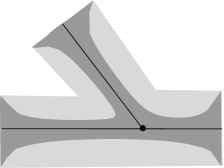
Figure 3. The original vertex neighbourhood ${V_{k}}(0)$ (light grey) and the shrunken vertex neighbourhood ${V_{k}}(\tau)$ (dark grey).

As in [P03, Sec. 7] we can show that the first eigenvalue of the Laplacian on ${V_{k}}(\tau)$ with Dirichlet boundary conditions except on the fixed boundary parts $\partial_{j}{V_{k}}(\tau)$, where we impose Neumann boundary conditions, tends to $\infty$, i.e.,

$$\lambda^{{\mathrm{D}}{\mathrm{N}}}_{1}({{V_{k}}(\tau)})\to\infty\qquad\text{as $\tau\to\infty$.}$$

Therefore there always exists a fixed $\tau\in(0,\infty)$ such that ${V_{k}}:={V_{k}}(\tau)$ satisfies (1.2). Fixing this shrinking parameter $\tau$, we proceed with the definition of ${M_{\varepsilon}}$ as in Section 2.

An example not satisfying the smallness assumption

Let us briefly give an example of a vertex neighbourhood not satisfying (1.2). For suitable vertex neighbourhoods (e.g. arising from the $\varepsilon$-neighbourhood of a graph) we will show the existence of an eigenvalue below the threshold $\lambda_{1}/\varepsilon^{2}=\pi^{2}/(4\varepsilon^{2})$ (cf. also  [SRW89] and [ABGM91] for the case of an $\varepsilon$-neighbourhood of a vertex with four infinite edges emanating (a “cross”); in the former reference one can also find a contour plot of the first eigenfunction). Therefore, the conclusion of Theorem 1.1 is false, i.e., (1.2) fails.

The existence of such an eigenvalue below the threshold can easily be established by inserting an appropriate trial function in the Rayleigh quotient. We consider a graph with one vertex and three adjacent edges of length $\ell$ and denote its $\varepsilon$-neighbourhood by ${M_{\varepsilon}}$. We decompose ${M_{\varepsilon}}$ into three rectangles ${U_{\varepsilon,j}}$ and three sets $A_{\varepsilon,j}$ as in Figure 4.

Figure 4. A simple trial function supported in a neighbourhood of the vertex has an eigenvalue below the threshold $\lambda_{1}/\varepsilon^{2}=\pi^{2}/(4\varepsilon^{2})$.

On the rectangle ${U_{\varepsilon,j}}$ we use the coordinates $0<x<\ell$ and $-\varepsilon<y<\varepsilon$ where $x=0$ corresponds to the common boundary with $A_{\varepsilon,j}$. We extend these coordinates from ${U_{\varepsilon,j}}$ onto $A_{\varepsilon,j}$ and define

$$u(x,y):=\varepsilon^{-1/2}\chi(x)\cos(\frac{\pi}{2\varepsilon}y)$$

as a test function on each of the three sets ${U_{\varepsilon,j}}\cup A_{\varepsilon,j}$. Here, $\chi(x)=1$ for $x<0$ (i.e., on $A_{\varepsilon,j}$), $\chi(x)=\cos(\pi x/(2\varepsilon\kappa))$ for $0\leq x\leq\kappa\varepsilon$ and $\chi(x)=0$ for $\varepsilon<x<\ell$ where $\kappa>0$ is some constant to be specified later. Although $u$ is not differentiable across the different borders (but continuous), it still lies in the quadratic form domain ${{\makebox[7.50002pt]{\raisebox{6.83331pt}{\hskip 1.93747pt$\scriptscriptstyle\circ$}}\makebox[0.0pt][r]{${\mathcal{H}}$}}{}^{1}({{M_{\varepsilon}}})}$.

A straightforward calculation yields

$$\frac{\|{du}\|^{2}_{{M_{\varepsilon}}}}{\|{u}\|^{2}_{{M_{\varepsilon}}}}-\frac{\pi^{2}}{4\varepsilon^{2}}=\Big{(}\frac{8\kappa\cos\alpha+3\pi^{2}\sin\alpha-16\kappa}{((3\pi^{2}-4)\cos\alpha+3\pi^{2}\kappa\sin\alpha+8)\kappa}\Big{)}\frac{\pi^{2}}{4\varepsilon^{2}}.$$ (5.1)

This quantity is negative for all $0<\alpha<0.93\pi$ if we choose e.g. $\kappa=3$. In particular, there exists a negative eigenvalue of $\Delta^{\mathrm{D}}_{{{M_{\varepsilon}}}}-\lambda_{1}/\varepsilon^{2}$ of order $\varepsilon^{-2}$, and Condition (1.2) fails here for any choice of vertex neighbourhoods ${V_{\varepsilon,k}}$ since the conclusion of Theorem 1.1 is false. Note that the vertex neighbourhoods ${V_{\varepsilon,k}}$ are not uniquely determined. One could enlarge ${V_{\varepsilon,k}}$ at each edge emanating by a cylinder of length $a\varepsilon$ taken away from the corresponding edge neighbourhood.

If $\Delta^{\mathrm{D}}_{{{M_{\varepsilon}}}}-\lambda_{1}/\varepsilon^{2}$ has negative eigenvalues it is not clear whether its appropriately scaled eigenvalues converge to eigenvalues of an operator on the graph $M_{0}$. The dependence of the leading order on the angle $\alpha$ in (5.1) indicates that the limit should depend on the angles of the edges meeting at a vertex.

References

- [ABGM91] Y. Avishai, D. Bessis, B. G. Giraud, and G. Mantica, Quantum bound states in open geometries, Phys. Rev. B 44 (1991), no. 15, 8028–8034.
- [Da96] E. B. Davies, Spectral theory and differential operators, Cambridge University Press, Cambridge, 1996.
- [DE95] P. Duclos and P. Exner, Curvature-induced bound states in quantum waveguides in two and three dimensions, Rev. Math. Phys. 7 (1995), no. 1, 73–102.
- [EP04] P. Exner and O. Post, Convergence of spectra of graph-like thin manifolds, to appear in Journal of Geometry and Physics (2004).
- [EŠ89] P. Exner and P. Šeba, Bound states in curved quantum waveguides, J. Math. Phys. 30 (1989), no. 11, 2574–2580.
- [K66] T. Kato, Perturbation theory for linear operators, Springer-Verlag, Berlin, 1966.
- [KaP88] L. Karp and M. Pinsky, First-order asymptotics of the principal eigenvalue of tubular neighborhoods, Geometry of random motion (Ithaca, N.Y., 1987), Contemp. Math., vol. 73, Amer. Math. Soc., Providence, RI, 1988, pp. 105–119.
- [KoS99] V. Kostrykin and R. Schrader, Kirchhoff’s rule for quantum wires, J. Phys. A 32 (1999), no. 4, 595–630.
- [Ku02] P. Kuchment, Graph models for waves in thin structures, Waves Random Media 12 (2002), no. 4, R1–R24.
- [Ku04] by same author, Quantum graphs: I. Some basic structures, Waves Random Media 14 (2004), S107–S128.
- [KuZ01] P. Kuchment and H. Zeng, Convergence of spectra of mesoscopic systems collapsing onto a graph, J. Math. Anal. Appl. 258 (2001), no. 2, 671–700.
- [KuZ03] by same author, Asymptotics of spectra of Neumann Laplacians in thin domains, Advances in differential equations and mathematical physics (Birmingham, AL, 2002), Contemp. Math., vol. 327, Amer. Math. Soc., Providence, RI, 2003, pp. 199–213.
- [P03] O. Post, Eigenvalues in spectral gaps of a perturbed periodic manifold, Mathematische Nachrichten 261–262 (2003), 141–162.
- [RuS53] K. Ruedenberg and C. W. Scherr, Free–electron network model for conjugated systems, I. Theory, J. Chem. Phys. 21 (1953), 1565–1581.
- [RS80] M. Reed and B. Simon, Methods of modern mathematical physics I: Functional analysis, Academic Press, New York, 1980.
- [RSc01] J. Rubinstein and M. Schatzman, Variational problems on multiply connected thin strips. I. Basic estimates and convergence of the Laplacian spectrum, Arch. Ration. Mech. Anal. 160 (2001), no. 4, 271–308.
- [SRW89] R. L. Schult, D. G. Ravenhall, and H. W. Wyld, Quantum bound states in a classically unbound system of crossed wires, Phys. Rev. B 39 (1989), no. 8, 5476–5479.