Computation of multiple eigenvalues and generalized eigenvectors for matrices dependent on parameters

Abstract

The paper develops Newton’s method of finding multiple eigenvalues with one Jordan block and corresponding generalized eigenvectors for matrices dependent on parameters. It computes the nearest value of a parameter vector with a matrix having a multiple eigenvalue of given multiplicity. The method also works in the whole matrix space (in the absence of parameters). The approach is based on the versal deformation theory for matrices. Numerical examples are given.

Keywords: multiparameter matrix family, multiple eigenvalue, generalized eigenvector, Jordan block, versal deformation, Schur decomposition

1 Introduction

Transformation of a square nonsymmetric (non-Hermitian) matrix $\mathbf{A}$ to the Jordan canonical form is the classical subject that finds various applications in pure and applied mathematics and natural sciences. It is well known that a generic matrix has only simple eigenvalues and its Jordan canonical form is a diagonal matrix. Nevertheless, multiple eigenvalues typically appear in matrix families, and one Jordan block is the most typical Jordan structure of a multiple eigenvalue [3, 4]. Many interesting and important phenomena associated with qualitative changes in the dynamics of mechanical systems [20, 29, 30, 36], stability optimization [6, 21, 25], and bifurcations of eigenvalues under matrix perturbations [32, 35, 34, 38] are related to multiple eigenvalues. Recently, multiple eigenvalues with one Jordan block became of great interest in physics, including quantum mechanics and nuclear physics [2, 17, 24], optics [5], and electrical engineering [8]. In most applications, multiple eigenvalues appear through the introduction of parameters.

In the presence of multiple eigenvalues, the numerical problem of computation of the Jordan canonical form is unstable, since the degenerate structure can be destroyed by arbitrarily small perturbations (caused, for example, by round-off errors). Hence, instead of analyzing a single matrix, we should consider this problem in some neighborhood in matrix or parameter space. Such formulation leads to the important problem left open by Wilkinson [40, 41]: to find the distance of a given matrix to the nearest degenerate matrix.

We study the problem of finding multiple eigenvalues for matrices dependent on several parameters. This implies that matrix perturbations are restricted to a specific submanifold in matrix space. Such restriction is the main difficulty and difference of this problem from the classical analysis in matrix spaces. Existing approaches for finding matrices with multiple eigenvalues [7, 9, 11, 12, 16, 18, 19, 23, 26, 33, 40, 41] assume arbitrary perturbations of a matrix and, hence, they do not work for multiparameter matrix families. We also mention the topological method for the localization of double eigenvalues in two-parameter matrix families [22].

In this paper, we develop Newton’s method for finding multiple eigenvalues with one Jordan block and corresponding generalized eigenvectors in multiparameter matrix families. The presented method solves numerically the Wilkinson problem of finding the nearest matrix with a multiple eigenvalue (both in multiparameter and matrix space formulations). The implementation of the method in MATLAB code is available, see [31]. The method is based on the versal deformation theory for matrices. In spirit, our approach is similar to [13], where matrices with multiple eigenvalues where found by path-following in matrix space (multiparameter case was not considered).

The paper is organized as follows. In Section 2, we introduce concepts of singularity theory and describe a general idea of the paper. Section 3 provides expressions for values and derivatives of versal deformation functions, which are used in Newton’s method in Section 4. Section 5 contains examples. In Section 6 we discuss convergence and accuracy of the method. Section 7 analyzes the relation of multiple eigenvalues with sensitivities of simple eigenvalues of perturbed matrices. In Conclusion, we summarize this contribution and discuss possible extensions of the method. Proofs are collected in the Appendix.

2 Multiple eigenvalues with one Jordan block in multiparameter matrix families

Let us consider an $m\times m$ complex non-Hermitian matrix $\mathbf{A}$, which is an analytical function of a vector of complex parameters $\mathbf{p}=(p_{1},\ldots,p_{n})$. Similarly, one can consider real or complex matrices smoothly dependent on real parameters, and we will comment the difference among these cases where appropriate. Our goal is to find the values of parameter vector $\mathbf{p}$ at which the matrix $\mathbf{A}(\mathbf{p})$ has an eigenvalue $\lambda$ of algebraic multiplicity $d$ with one $d\times d$ Jordan block (geometric multiplicity $1$). Such and eigenvalue $\lambda$ is called nonderogatory. There is a Jordan chain of generalized vectors $\mathbf{u}_{1},\ldots,\mathbf{u}_{d}$ (the eigenvector and associated vectors) corresponding to $\lambda$ and determined by the equations

$$\begin{array}[]{rcl}\mathbf{A}\mathbf{u}_{1}&=&\lambda\mathbf{u}_{1},\\[3.0pt] \mathbf{A}\mathbf{u}_{2}&=&\lambda\mathbf{u}_{2}+\mathbf{u}_{1},\\[3.0pt] &\vdots&\\[3.0pt] \mathbf{A}\mathbf{u}_{d}&=&\lambda\mathbf{u}_{d}+\mathbf{u}_{d-1}.\end{array}$$ (2.1)

These vectors form an $m\times d$ matrix $\mathbf{U}=[\mathbf{u}_{1},\ldots,\mathbf{u}_{d}]$ satisfying the equation

$$\mathbf{A}\mathbf{U}=\mathbf{U}\mathbf{J}_{\lambda},\qquad\mathbf{J}_{\lambda}=\left(\begin{array}[]{cccc}\lambda&1&&\\ &\lambda&\ddots&\\ &&\ddots&1\\ &&&\lambda\end{array}\right),$$ (2.2)

where $\mathbf{J}_{\lambda}$ is the Jordan block of size $d$. Recall that the Jordan chains taken for all the eigenvalues and Jordan blocks determine the transformation of the matrix $\mathbf{A}$ to the Jordan canonical form [14].

In singularity theory [4], parameter space is divided into a set of strata (smooth submanifolds of different dimensions), which correspond to different Jordan structures of the matrix $\mathbf{A}$. Consider, for example the matrix family

$$\mathbf{A}(\mathbf{p})=\left(\begin{array}[]{cccc}0&1&0&0\\ p_{1}&0&1&0\\ p_{2}&0&0&1\\ p_{3}&0&0&0\end{array}\right),\quad\mathbf{p}=(p_{1},p_{2},p_{3}).$$ (2.3)

The bifurcation diagram in parameter space is shown in Figure 1 (for simplicity, we consider only real values of parameters). There are four degenerate strata: $\lambda^{2}$ (surfaces), $\lambda^{3}$ and $\lambda_{1}^{2}\lambda_{2}^{2}$ (curves), and $\lambda^{4}$ (a point). The surface $\lambda^{2}$, curve $\lambda^{3}$, and point $\lambda^{4}$ correspond, respectively, to the matrices with double, triple, and quadruple eigenvalues with one Jordan block. The curve $\lambda_{1}^{2}\lambda_{2}^{2}$ is the transversal self-intersection of the stratum $\lambda^{2}$ corresponding to the matrices having two different double eigenvalues. This bifurcation diagram represents the well-known “swallow tail” singularity [4].

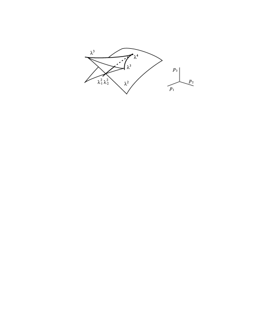
Figure 1: Geometry of the bifurcation diagram.

We study the set of parameter vectors, denoted by $\lambda^{d}$, corresponding to matrices having multiple eigenvalues with one Jordan block of size $d$. The set $\lambda^{d}$ is a smooth surface in parameter space having codimension $d-1$ [3, 4]. Thus, the problem of finding multiple eigenvalues in a matrix family is equivalent to finding the surface $\lambda^{d}$ or its particular point. Since the surface $\lambda^{d}$ is smooth, we can find it numerically by using Newton’s method. This requires describing the surface $\lambda^{d}$ as a solution of $d-1$ equations

$$q_{i}(\mathbf{p})=0,\qquad i=2,\ldots,d,$$ (2.4)

for independent smooth functions $q_{i}(\mathbf{p})$. (In these notations, we keep the first function for the multiple eigenvalue $\lambda=q_{1}(\mathbf{p})$.) Finding the functions $q_{i}(\mathbf{p})$ and their first derivatives is the clue to the problem solution.

In this paper, we define the functions $q_{i}(\mathbf{p})$ in the following way. According to versal deformation theory [3, 4], in the neighborhood of $\lambda^{d}$, the matrix $\mathbf{A}(\mathbf{p})$ satisfies the relation

$$\mathbf{A}(\mathbf{p})\mathbf{U}(\mathbf{p})=\mathbf{U}(\mathbf{p})\mathbf{B}(\mathbf{p}),\quad\mathbf{B}(\mathbf{p})=\left(\begin{array}[]{cccc}q_{1}(\mathbf{p})&1&&\\ q_{2}(\mathbf{p})&q_{1}(\mathbf{p})&\ddots&\\ \vdots&&\ddots&1\\ q_{d}(\mathbf{p})&&&q_{1}(\mathbf{p})\end{array}\right),$$ (2.5)

where $\mathbf{U}(\mathbf{p})$ is an $m\times d$ analytic matrix family, and $q_{1}(\mathbf{p}),\ldots,q_{d}(\mathbf{p})$ are analytic functions (blank places in the matrix are zeros). The functions $q_{1}(\mathbf{p}),\ldots,q_{d}(\mathbf{p})$ are uniquely determined by the matrix family $\mathbf{A}(\mathbf{p})$.

By using (2.5), it is straightforward to see that the surface $\lambda^{d}$ is defined by equations (2.4). If (2.4) are satisfied, the matrix $\mathbf{B}(\mathbf{p})$ is the $d\times d$ Jordan block. Hence, at $\mathbf{p}\in\lambda^{d}$, the multiple eigenvalue is $\lambda=q_{1}(\mathbf{p})$ and the columns of $\mathbf{U}(\mathbf{p})$ are the generalized eigenvectors satisfying equations (2.1). The method of finding the functions $q_{i}(\mathbf{p})$ and $\mathbf{U}(\mathbf{p})$ and their derivatives at the point $\mathbf{p}\in\lambda^{d}$ has been developed in [27, 28]. In Newton’s method for solving (2.4), we need the values and derivatives of the functions $q_{i}(\mathbf{p})$ at an arbitrary point $\mathbf{p}\notin\lambda^{d}$.

3 Linearization of versal deformation functions

Let $\mathbf{p}_{0}$ be a given parameter vector determining a matrix $\mathbf{A}_{0}=\mathbf{A}(\mathbf{p}_{0})$. Since multiple eigenvalues are nongeneric, we typically deal with a diagonalizable matrix $\mathbf{A}_{0}$. Let $\lambda_{1},\ldots,\lambda_{m}$ be eigenvalues of the matrix $\mathbf{A}_{0}$. We sort these eigenvalues so that the first $d$ of them, $\lambda_{1},\ldots,\lambda_{d}$, coalesce as the parameter vector is transferred continuously to the surface $\lambda^{d}$. The eigenvalues that form a multiple eigenvalue are usually known from the context of a particular problem. Otherwise, one can test different sets of $d$ eigenvalues.

Let us choose $m\times d$ matrices $\mathbf{X}$ and $\mathbf{Y}$ such that

$$\mathbf{A}_{0}\mathbf{X}=\mathbf{X}\mathbf{S},\quad\mathbf{Y}^{*}\mathbf{A}_{0}=\mathbf{S}\mathbf{Y}^{*},\quad\mathbf{Y}^{*}\mathbf{X}=\mathbf{I},$$ (3.1)

where $\mathbf{S}$ is the $d\times d$ matrix whose eigenvalues are $\lambda_{1},\ldots,\lambda_{d}$; the star denotes the complex conjugate transpose. The first two equalities in (3.1) imply that the columns of the matrix $\mathbf{X}$ span the right invariant subspace of $\mathbf{A}_{0}$ corresponding to $\lambda_{1},\ldots,\lambda_{d}$, and the columns of $\mathbf{Y}$ span the left invariant subspace. The third equality is the normalization condition. The matrix $\mathbf{S}$ can be expressed as

$$\mathbf{S}=\mathbf{Y}^{*}\mathbf{A}_{0}\mathbf{X},$$ (3.2)

which means that $\mathbf{S}$ is the restriction of the matrix operator $\mathbf{A}_{0}$ to the invariant subspace given by the columns of $\mathbf{X}$. The constructive way of choosing the matrices $\mathbf{S}$, $\mathbf{X}$, and $\mathbf{Y}$ will be described in the next section.

The following theorem provides the values and derivatives of the functions $q_{1}(\mathbf{p}),\ldots,q_{d}(\mathbf{p})$ in the versal deformation (2.5) at the point $\mathbf{p}_{0}$.

Theorem 3.1

Let $\mathbf{S}$, $\mathbf{Y}$, and $\mathbf{X}$ be the matrices satisfying equations (3.1). Then

$$q_{1}(\mathbf{p}_{0})=\mathrm{trace}\,\mathbf{S}/d,$$ (3.3)

and the values of $q_{2}(\mathbf{p}_{0}),\ldots,q_{d}(\mathbf{p}_{0})$ are found as the characteristic polynomial coefficients of the traceless matrix $\mathbf{S}-q_{1}(\mathbf{p}_{0})\mathbf{I}$:

$$z^{d}-q_{2}(\mathbf{p}_{0})z^{d-2}-\cdots-q_{d-1}(\mathbf{p}_{0})z-q_{d}(\mathbf{p}_{0})=\det\big{(}(z+q_{1}(\mathbf{p}_{0}))\mathbf{I}-\mathbf{S}\big{)},$$ (3.4)

where $\mathbf{I}$ is the $d\times d$ identity matrix. The first derivatives of the functions $q_{i}(\mathbf{p})$ at $\mathbf{p}_{0}$ are determined by the recurrent formulae

$$\begin{array}[]{l}\displaystyle\frac{\partial q_{1}}{\partial p_{j}}=\mathrm{trace}\left(\mathbf{Y}^{*}\frac{\partial\mathbf{A}}{\partial p_{j}}\mathbf{X}\right)/d,\\[10.0pt] \displaystyle\frac{\partial q_{i}}{\partial p_{j}}=\mathrm{trace}\left((\mathbf{S}-q_{1}(\mathbf{p}_{0})\mathbf{I})^{i-1}\mathbf{Y}^{*}\frac{\partial\mathbf{A}}{\partial p_{j}}\mathbf{X}\right)-\mathrm{trace}(\mathbf{C}^{i-1})\frac{\partial q_{1}}{\partial p_{j}}-\sum_{k=2}^{i-1}\mathrm{trace}(\mathbf{C}^{i-1}\mathbf{E}_{k1})\frac{\partial q_{k}}{\partial p_{j}},\\[15.0pt] i=2,\ldots,d,\quad j=1,\ldots,n,\end{array}$$ (3.5)

where the derivatives are evaluated at $\mathbf{p}_{0}$; $\mathbf{C}=\mathbf{B}(\mathbf{p}_{0})-q_{1}(\mathbf{p}_{0})\mathbf{I}$ is the companion matrix

$$\mathbf{C}=\left(\begin{array}[]{cccc}0&1&&\\ q_{2}(\mathbf{p}_{0})&0&\ddots&\\ \vdots&&\ddots&1\\ q_{d}(\mathbf{p}_{0})&&&0\end{array}\right)=\mathbf{J}_{0}+\sum_{i=2}^{d}q_{i}(\mathbf{p}_{0})\mathbf{E}_{i1},$$ (3.6)

and $\mathbf{E}_{i1}$ is the matrix having the unit $(i,1)$th element and zeros in other places.

The proof of this theorem is given in the Appendix.

When the matrix $\mathbf{A}$ is arbitrary (not restricted to a multiparameter matrix family), each entry of the matrix can be considered is an independent parameter. Hence, the matrix $\mathbf{A}$ can be used instead of the parameter vector: $\mathbf{p}\longrightarrow\mathbf{A}$. The derivative of $\mathbf{A}$ with respect to its $(i,j)$th entry is $\mathbf{E}_{ij}$. Thus, the formulae of Theorem 3.1 can be applied.

Corollary 3.1

Let $\mathbf{S}$, $\mathbf{Y}$, and $\mathbf{X}$ be the matrices satisfying equations (3.1). Then the values of $q_{1}(\mathbf{A}_{0}),\ldots,q_{d}(\mathbf{A}_{0})$ are given by formulae (3.3) and (3.4) with $\mathbf{p}_{0}$ substituted by $\mathbf{A}_{0}$. Derivatives of the functions $q_{1}(\mathbf{A}),\ldots,q_{d}(\mathbf{A})$ with respect to components of the matrix $\mathbf{A}$ taken at $\mathbf{A}_{0}$ are

$$\begin{array}[]{l}\displaystyle\frac{\partial q_{1}}{\partial\mathbf{A}}=\left(\mathbf{X}\mathbf{Y}^{*}/d\right)^{T},\\[10.0pt] \displaystyle\frac{\partial q_{i}}{\partial\mathbf{A}}=\left(\mathbf{X}(\mathbf{S}-q_{1}(\mathbf{p}_{0})\mathbf{I})^{i-1}\mathbf{Y}^{*}\right)^{T}-\mathrm{trace}(\mathbf{C}^{i-1})\frac{\partial q_{1}}{\partial\mathbf{A}}-\sum_{k=2}^{i-1}\mathrm{trace}(\mathbf{C}^{i-1}\mathbf{E}_{k1})\frac{\partial q_{k}}{\partial\mathbf{A}},\\[3.0pt] \qquad\quad i=2,\ldots,d.\end{array}$$ (3.7)

Here $T$ is the transpose operator, and

$$\frac{\partial q_{i}}{\partial\mathbf{A}}=\left(\begin{array}[]{ccc}\displaystyle\frac{\partial q_{i}}{\partial a_{11}}&\cdots&\displaystyle\frac{\partial q_{i}}{\partial a_{1m}}\\[10.0pt] \vdots&\ddots&\vdots\\[3.0pt] \displaystyle\frac{\partial q_{i}}{\partial a_{m1}}&\cdots&\displaystyle\frac{\partial q_{i}}{\partial a_{mm}}\end{array}\right)$$ (3.8)

is the $m\times m$ matrix of derivatives of $q_{i}(\mathbf{A})$ with respect to components of the matrix $\mathbf{A}$ taken at $\mathbf{A}_{0}$.

At $\mathbf{p}_{0}\in\lambda^{d}$, we can find the multiple eigenvalue $\lambda$ and the corresponding Jordan chain of generalized eigenvectors $\mathbf{u}_{1},\ldots,\mathbf{u}_{d}$. This problem reduces to the transformation of the matrix $\mathbf{S}$ to the prescribed Jordan form (one Jordan block). A possible way of solving this problem is presented in the following theorem (see the Appendix for the proof.).

Theorem 3.2

At the point $\mathbf{p}_{0}\in\lambda^{d}$, the multiple eigenvalue is given by the expression

$$\lambda=\mathrm{trace}\,\mathbf{S}/d.$$ (3.9)

The general form of the Jordan chain of generalized eigenvectors $\mathbf{u}_{1},\ldots,\mathbf{u}_{d}$ is

$$\mathbf{u}_{1}=\mathbf{X}(\mathbf{S}-\lambda\mathbf{I})^{d-1}\mathbf{k},\quad\ldots,\quad\mathbf{u}_{d-1}=\mathbf{X}(\mathbf{S}-\lambda\mathbf{I})\mathbf{k},\ \ \mathbf{u}_{d}=\mathbf{X}\mathbf{k},$$ (3.10)

where $\mathbf{k}\in\mathbb{C}^{d}$ is an arbitrary vector such that the eigenvector $\mathbf{u}_{1}$ is nonzero. Choosing a particular unit-norm eigenvector $\hat{\mathbf{u}}_{1}$, e.g., by taking the scaled biggest norm column of the matrix $\mathbf{X}(\mathbf{S}-\lambda\mathbf{I})^{d-1}$, one can fix the vector $\mathbf{k}$ by the orthonormality conditions

$$\hat{\mathbf{u}}_{1}^{*}\mathbf{u}_{i}=\left\{\begin{array}[]{ll}1,&i=1;\\ 0,&i=2,\ldots,d.\end{array}\right.$$ (3.11)

The accuracy of the multiple eigenvalue and generalized eigenvectors determined by formulae (3.9) and (3.10) has the same order as the accuracy of the point $\mathbf{p}_{0}$ in the surface $\lambda^{d}$.

4 Newton’s method

There are several ways to find the matrices $\mathbf{S}$, $\mathbf{X}$, and $\mathbf{Y}$. The simplest way is to use the diagonalization of $\mathbf{A}_{0}$. Then $\mathbf{S}=\mathrm{diag}(\lambda_{1},\ldots,\lambda_{d})$ is the diagonal matrix, and the columns of $\mathbf{X}$ and $\mathbf{Y}$ are the right and left eigenvectors corresponding to $\lambda_{1},\ldots,\lambda_{d}$. This way will be discussed in Section 5.

If the parameter vector $\mathbf{p}_{0}$ is close to the surface $\lambda^{d}$, the diagonalization of the matrix $\mathbf{A}_{0}$ is ill-conditioned. Instead of the diagonalization, one can use the numerically stable Schur decomposition $\widetilde{\mathbf{S}}=\widetilde{\mathbf{X}}^{*}\mathbf{A}_{0}\widetilde{\mathbf{X}}$, where $\widetilde{\mathbf{S}}$ is an upper-triangular matrix called the Schur canonical form, and $\widetilde{\mathbf{X}}=(\widetilde{\mathbf{X}}^{*})^{-1}$ is a unitary matrix [15]. The diagonal elements $\widetilde{s}_{11},\ldots,\widetilde{s}_{mm}$ of $\widetilde{\mathbf{S}}$ are the eigenvalues of $\mathbf{A}_{0}$. We can choose the Schur form so that the first $d$ diagonal elements are the eigenvalues $\lambda_{1},\ldots,\lambda_{d}$. Performing the block-diagonalization of the Schur form $\widetilde{\mathbf{S}}$ [15, §7.6], we obtain the block-diagonal matrix

$$\left(\begin{array}[]{cc}\mathbf{S}&0\\ 0&\mathbf{S}^{\prime}\end{array}\right)=[\mathbf{Y},\mathbf{Y}^{\prime}]^{*}\mathbf{A}_{0}[\mathbf{X},\mathbf{X}^{\prime}],$$ (4.1)

where $\mathbf{S}$ is a $d\times d$ upper-triangular matrix with the diagonal $(\lambda_{1},\ldots,\lambda_{d})$; $[\mathbf{X},\mathbf{X}^{\prime}]$ and $[\mathbf{Y},\mathbf{Y}^{\prime}]^{*}=[\mathbf{X},\mathbf{X}^{\prime}]^{-1}$ are nonsingular $m\times m$ matrices (not necessarily unitary). These operations with a Schur canonical form are standard and included in many numerical linear algebra packages, for example, LAPACK [1]. They are numerically stable if the eigenvalues $\lambda_{1},\ldots,\lambda_{d}$ are separated from the remaining part of the spectrum. As a result, we obtain the matrices $\mathbf{S}$, $\mathbf{X}$, and $\mathbf{Y}$ satisfying equations (3.1).

When the matrices $\mathbf{S}$, $\mathbf{X}$, and $\mathbf{Y}$ are determined, Theorem 3.1 provides the necessary information for using Newton’s method for determining the stratum $\lambda^{d}$. Indeed, having the parameter vector $\mathbf{p}_{0}=(p_{1}^{0},\ldots,p_{n}^{0})$ as the initial guess, we linearize equations (2.4) of the surface $\lambda^{d}$ as

$$q_{i}(\mathbf{p}_{0})+\sum_{j=1}^{n}\frac{\partial q_{i}}{\partial p_{j}}(p_{j}-p_{j}^{0})=0,\quad i=2,\ldots,d,$$ (4.2)

where the values of $q_{i}(\mathbf{p}_{0})$ and the derivatives $\partial q_{i}/\partial p_{j}$ at $\mathbf{p}_{0}$ are provided by Theorem 3.1. In the generic case, the linear part in (4.2) is given by the maximal rank matrix $[\partial q_{i}/\partial p_{j}]$. System (4.2) has the single solution if the number of parameters $n=d-1$ (the set $\lambda^{d}$ is an isolated point). If $n>d-1$, one can take the least squares solution or any other solution depending on which point of the surface $\lambda^{d}$ one would like to find. If $n<d$, the multiple eigenvalue still can exist in matrices with symmetries (e.g., Hamiltonian or reversible matrices [35]); then the least squares fit solution of (4.2) is a good choice.

In Newton’s method, the obtained vector of parameters $\mathbf{p}=(p_{1},\ldots,p_{n})$ is used in the next iteration. In each iteration, we should choose $d$ eigenvalues of the matrix $\mathbf{A}_{0}$. These are the $d$ eigenvalues nearest to the approximate multiple eigenvalue

$$\lambda=q_{1}(\mathbf{p}_{0})+\sum_{j=1}^{n}\frac{\partial q_{1}}{\partial p_{j}}(p_{j}-p_{j}^{0})$$ (4.3)

calculated at the previous step. If the iteration procedure converges, we obtain a point $\mathbf{p}\in\lambda^{d}$. Then the multiple eigenvalue and corresponding generalized eigenvectors are found by Theorem 3.2. Note that, at the point $\mathbf{p}\in\lambda^{d}$, system (4.2) determines the tangent plane to the surface $\lambda^{d}$ in parameter space. The pseudo-code of the described iteration procedure is presented in Table 1. Depending on a particular application, the line 3 in this pseudo-code can be implemented in different ways, e.g., as the least squares solution or as the solution nearest to the input parameter vector $\mathbf{p}_{0}$. The implementation of this method in MATLAB code is available, see [31].

INPUT: matrix family $\mathbf{A}(\mathbf{p})$, initial parameter vector $\mathbf{p}_{0}$, and eigenvalues $\lambda_{1},\ldots,\lambda_{d}$

1:	Schur decomposition and block-diagonalization (4.1) of the matrix $\mathbf{A}_{0}=\mathbf{A}(\mathbf{p}_{0})$;
2:	evaluate $q_{i}(\mathbf{p}_{0})$ and $\partial q_{i}/\partial p_{j}$ by formulae (3.3)–(3.5);
3:	find $\mathbf{p}_{new}$ by solving system (4.2) (e.g. the least squares solution);
4:	IF $\|\mathbf{p}_{new}-\mathbf{p}_{0}\|>\mathrm{desired\ accuracy}$
5:	evaluate approximate multiple eigenvalue $\lambda_{app}$ by (4.3);
6:	choose $d$ eigenvalues $\lambda_{1}^{new},\ldots,\lambda_{d}^{new}$ of $\mathbf{A}_{new}=\mathbf{A}(\mathbf{p}_{new})$ nearest to $\lambda_{app}$;
7:	perform a new iteration with $\mathbf{p}_{0}=\mathbf{p}_{new}$ and $\lambda_{i}=\lambda_{i}^{new}$, $i=1,\ldots,d$ (GOTO 1);
8:	ELSE (IF $\|\mathbf{p}_{new}-\mathbf{p}_{0}\|\leq\mathrm{desired\ accuracy}$)
9:	find multiple eigenvalue and generalized eigenvectors by formulae (3.9)–(3.11);

OUTPUT: parameter vector $\mathbf{p}\in\lambda^{d}$, multiple eigenvalue $\lambda$ and Jordan chain

of generalized eigenvectors $\mathbf{u}_{1},\ldots,\mathbf{u}_{d}$

Table 1: Pseudo-code of Newton’s method for finding multiple eigenvalues in multiparameter matrix families.

In case of complex matrices dependent on real parameters, the same formulae can be used. In this case, system (4.2) represents $2(d-1)$ independent equations (each equality determines two equations for real and imaginary parts). This agrees with the fact that the codimension of $\lambda^{d}$ in the space of real parameters is $2(d-1)$ [4].

Finally, consider real matrices smoothly dependent on real parameters. For complex multiple eigenvalues, the system (4.2) contains $2(d-1)$ independent real equations (codimension of $\lambda^{d}$ is $2(d-1)$). Remark that imaginary parts of the eigenvalues $\lambda_{1},\ldots,\lambda_{d}$ should have the same sign. For real multiple eigenvalues, $q_{i}(\mathbf{p}_{0})$ and $\partial q_{i}/\partial p_{j}$ are real (the real Schur decomposition must be used). Hence, (4.2) contains $d-1$ real equations (codimension of $\lambda^{d}$ is $d-1$). In this case, the eigenvalues $\lambda_{1},\ldots,\lambda_{d}$ are real or appear in complex conjugate pairs.

In some applications, like stability theory [35], we are interested in specific multiple eigenvalues, e.g., zero and purely imaginary eigenvalues. In this case equation (4.3) should be included in the linear system of Newton’s approximation (4.2).

For arbitrary matrices $\mathbf{A}=[a_{ij}]$ (without parameters), similar Newton’s iteration procedure is based on Corollary 3.1. The linearized equations (4.2) are substituted by

$$q_{i}(\mathbf{p}_{0})+\sum_{j,k=1}^{m}\frac{\partial q_{i}}{\partial a_{jk}}(a_{jk}-a_{jk}^{0})=0,\quad i=2,\ldots,d,$$ (4.4)

where $\mathbf{A}_{0}=[a_{jk}^{0}]$ is the matrix obtained at the previous step or the initial input matrix. The first-order approximation of the multiple eigenvalue (4.3) takes the form

$$\lambda=q_{1}(\mathbf{p}_{0})+\sum_{j,k=1}^{m}\frac{\partial q_{1}}{\partial a_{jk}}(a_{jk}-a_{jk}^{0}).$$ (4.5)

5 Examples

All calculations in the following examples were performed using MATLAB code [31]. For the sake of brevity, we will show only first several digits of the computation results.

5.1 Example 1

Let us consider the two-parameter family of real matrices

$$\mathbf{A}(\mathbf{p})=\left(\begin{array}[]{ccc}1&3&0\\ p_{1}&1&p_{2}\\ 2&3&1\end{array}\right),\quad\mathbf{p}=(p_{1},p_{2}).$$ (5.1)

Bifurcation diagram for this matrix family is found analytically by studying the discriminant of the characteristic polynomial. There are two smooth curves $\lambda^{2}$ and a point $\lambda^{3}$ at the origin (the cusp singularity), see Figure 2.

Let us consider the point $\mathbf{p}_{0}=(-0.03,8.99)$, where the matrix $\mathbf{A}_{0}$ has the eigenvalues $\lambda_{1,2}=-1.995\pm i0.183$ and $\lambda_{3}=6.990$. In order to detect a double real eigenvalue, we choose the pair of complex conjugate eigenvalues $\lambda_{1}$, $\lambda_{2}$. By ordering diagonal blocks in the real Schur form of $\mathbf{A}_{0}$ and block-diagonalizing, we find the matrices $\mathbf{S}$, $\mathbf{X}$, and $\mathbf{Y}$ satisfying (3.1) in the form

$$\mathbf{S}=\left(\begin{array}[]{cc}-1.995&-5.083\\ 0.007&-1.995\end{array}\right),\ \mathbf{X}=\left(\begin{array}[]{cc}0.688&-0.676\\ -0.688&-0.491\\ 0.231&0.550\end{array}\right),\ \mathbf{Y}=\left(\begin{array}[]{cc}0.729&-0.574\\ -0.604&-0.286\\ 0.357&0.858\end{array}\right).$$

Applying the formulae of Theorem 3.1, we find

$$\left(\begin{array}[]{c}q_{1}(\mathbf{p}_{0})\\[2.0pt] q_{2}(\mathbf{p}_{0})\end{array}\right)=\left(\begin{array}[]{c}-1.995\\ -0.033\end{array}\right),\quad\left(\begin{array}[]{cc}\partial q_{1}/\partial p_{1}&\partial q_{1}/\partial p_{2}\\[2.0pt] \partial q_{2}/\partial p_{1}&\partial q_{2}/\partial p_{2}\end{array}\right)=\left(\begin{array}[]{cc}-0.111&-0.148\\ 1.001&0.333\end{array}\right).$$ (5.2)

The linearized system (4.2) represents one real scalar equation. We find the nearest parameter vector $\mathbf{p}\in\lambda^{2}$ (the least squares solution) as

$$\mathbf{p}=\mathbf{p}_{0}-\frac{q_{2}(\mathbf{p}_{0})}{(\partial q_{2}/\partial p_{1})^{2}+(\partial q_{2}/\partial p_{2})^{2}}\,(\partial q_{2}/\partial p_{1},\,\partial q_{2}/\partial p_{2})=(-0.00001,8.99999).$$ (5.3)

After five iterations of Newton’s method, we find the exact nearest point $\mathbf{p}=(0,\,9)\in\lambda^{2}$. Then Theorem 3.2 gives the multiple eigenvalue and the Jordan chain with the accuracy $10^{-15}$:

$$\lambda=-2,\quad[\mathbf{u}_{1},\mathbf{u}_{2}]=\frac{1}{\sqrt{19}}\left(\begin{array}[]{cc}3&-1+30/19\\ -3&2-30/19\\ 1&-1+10/19\end{array}\right).$$ (5.4)

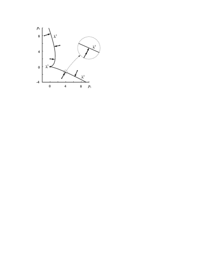
Figure 2: One-step approximations of the nearest points with double eigenvalues.

Now let us take different points $\mathbf{p}_{0}$ in the neighborhood of the curve $\lambda^{2}$ and calculate one-step Newton’s approximations of the nearest points $\mathbf{p}\in\lambda^{2}$. In this case we choose $\lambda_{1},\,\lambda_{2}$ as a pair of complex conjugate eigenvalues of $\mathbf{A}_{0}=\mathbf{A}(\mathbf{p}_{0})$. If all eigenvalues of $\mathbf{A}_{0}$ are real, we test all different pairs of eigenvalues, and take the pair providing the nearest point $\mathbf{p}\in\lambda^{2}$. The result is shown in Figure 2, where each arrow connects the initial point $\mathbf{p}_{0}$ with the one-step Newton’s approximation $\mathbf{p}$. For one point $\mathbf{p}_{0}$ we performed two iterations, taking the point $\mathbf{p}$ as a new initial point $\mathbf{p}_{0}=\mathbf{p}$. The convergence of this iteration series is shown in the enlarged part of parameter space (inside the circle in Figure 2). The results confirm Newton’s method rate of convergence.

5.2 Example 2

Let us consider the real matrix $\mathbf{A}_{0}=\mathbf{A}_{1}+\varepsilon\mathbf{E}$, where

$$\mathbf{A}_{1}=\left(\begin{array}[]{ccc}0&1&0\\ 0&0&\delta\\ 0&0&0\end{array}\right),\quad\mathbf{E}=\left(\begin{array}[]{ccc}3&4&2\\ 8&3&6\\ 4&9&6\end{array}\right),$$ (5.5)

and $\varepsilon=\textrm{2.2e-15}$, $\delta=\textrm{1.5e-9}$. This matrix was used in [10] for testing the GUPTRI [18, 19] algorithm. It turned out that this algorithm detects a matrix $\mathbf{A}\in\lambda^{3}$ (with a nonderogatory triple eigenvalue) at the distance $O(10^{-6})$ from $\mathbf{A}_{0}$, while the distance from $\mathbf{A}_{0}$ to $\lambda^{3}$ is less than $\|\varepsilon\mathbf{E}\|_{F}=\textrm{3.62e-14}$ since $\mathbf{A}_{1}\in\lambda^{3}$. This is explained by the observation that the algorithm finds matrix perturbations along a specific set of directions, and these directions are almost tangent to the stratum $\lambda^{3}$ in the case under consideration [10].

Our method determines locally the whole stratum $\lambda^{3}$ in matrix space and, hence, it should work correctly in this case. Since the triple eigenvalue is formed by all eigenvalues of $\mathbf{A}_{0}$, we can use $\mathbf{S}=\mathbf{A}_{0}$ and $\mathbf{X}=\mathbf{Y}=\mathbf{I}$ in the formulae of Corollary 3.1. As a result, we find the least squares solution of system (4.4) in the form $\mathbf{A}=\mathbf{A}_{0}+\Delta\mathbf{A}$, where

$$\Delta\mathbf{A}=\textrm{1.0e-14}*\left(\begin{array}[]{ccc}0&0&0\\ -1.760&0&0\\ -0.880&0&0\end{array}\right).$$ (5.6)

Approximations of the multiple eigenvalue and corresponding generalized eigenvectors evaluated by Theorem 3.2 for the matrix $\mathbf{A}$ are

$$\lambda=\textrm{8.800e-15},\quad[\mathbf{u}_{1},\,\mathbf{u}_{2},\,\mathbf{u}_{3}]=\left(\begin{array}[]{ccc}1.000&-0.000&-0.000\\ 0.000&1.000&-0.000\\ 0.000&0.000&\textrm{6.667e+8}\end{array}\right).$$ (5.7)

We detected the matrix $\mathbf{A}$ at the distance $\|\Delta\mathbf{A}\|_{F}=\textrm{1.97e-14}$, which is smaller than the initial perturbation $\|\varepsilon\mathbf{E}\|_{F}=\textrm{3.62e-14}$ ($\|\Delta\mathbf{A}\|_{F}$ denotes the Frobenius matrix norm). The matrix $\mathbf{U}=[\mathbf{u}_{1},\mathbf{u}_{2},\mathbf{u}_{3}]$ satisfies the Jordan chain equation (2.2) with the very high accuracy $\|\mathbf{A}\mathbf{U}-\mathbf{U}\mathbf{J}_{\lambda}\|_{F}/\|\mathbf{U}\|_{F}=\textrm{9.6e-23}$.

The normal complementary subspace $N$ of the tangent space to $\lambda^{3}$ at $\mathbf{A}_{1}$ has the form [4]

$$N=\bigg{\{}\left(\begin{array}[]{ccc}0&0&0\\ x&0&0\\ y&\delta x&0\end{array}\right)\mid\ x,y\in\mathbb{R}\bigg{\}}.$$ (5.8)

It is easy to see that the matrix $\Delta\mathbf{A}$ in (5.6) is equal to the projection of $\,-\varepsilon\mathbf{E}$ to the normal subspace $N$. This confirms that the obtained matrix $\mathbf{A}\in\lambda^{3}$ is the nearest to $\mathbf{A}_{0}$.

5.3 Example 3

Let us consider the $12\times 12$ Frank matrix $\mathbf{A}_{0}=[a_{ij}^{0}]$ with the elements

$$a_{ij}^{0}=\left\{\begin{array}[]{ll}n+1-\max(i,j),&j\geq i-1,\\ 0,&j<i-1.\end{array}\right.$$ (5.9)

The Frank matrix has six small positive eigenvalues which are ill-conditioned and form nonderogatory multiple eigenvalues of multiplicities $d=2,\ldots,6$ for small perturbations of the matrix. The results obtained by Newton’s method with the use of Corollary 3.1 are presented in Table 2. An eigenvalue of multiplicity $d$ of the nearest matrix $\mathbf{A}\in\lambda^{d}$ is formed by $d$ smallest eigenvalues of $\mathbf{A}_{0}$. The second column of Table 2 gives the distance $\mathrm{dist}(\mathbf{A}_{0},\lambda^{d})=\|\mathbf{A}-\mathbf{A}_{0}\|_{F}$, where the matrix $\mathbf{A}$ is computed after one step of Newton’s procedure. The third column provides exact distances computed by Newton’s method, which requires 4–5 iterations to find the distance with the accuracy $O(10^{-15})$. At each iteration, we find the solution $\mathbf{A}$ of system (4.4), which is the nearest to the matrix (5.9). The multiple eigenvalues and corresponding generalized eigenvectors are found at the last iteration by Theorem 3.2. The accuracy estimated as $\|\mathbf{A}\mathbf{U}-\mathbf{U}\mathbf{J}_{\lambda}\|_{F}/\|\mathbf{U}\|_{F}$ varies between $10^{-10}$ and $10^{-13}$. The matrices of generalized eigenvectors $\mathbf{U}$ have small condition numbers, which are given in the fourth column of Table 2. For comparison, the fifth and sixth columns give upper bounds for the distance to the nearest matrix $\mathbf{A}\in\lambda^{d}$ found in [13, 18].

$d$	$\begin{array}[]{c}\textrm{dist}(\mathbf{A}_{0},\lambda^{d})\\ \textrm{1-step approximation}\end{array}$	$\begin{array}[]{c}\textrm{dist}(\mathbf{A}_{0},\lambda^{d})\\ \textrm{exact}\end{array}$	cond $\mathbf{U}$	$\|\mathbf{A}-\mathbf{A}_{0}\|_{F}$ [13]	$\|\mathbf{A}-\mathbf{A}_{0}\|_{F}$ [18]
2	1.619e-10	1.850e-10	1.125	3.682e-10
3	1.956e-8	2.267e-8	1.746	3.833e-8
4	1.647e-6	1.861e-6	4.353	3.900e-6
5	9.299e-5	1.020e-4	14.14	4.280e-4	6e-3
6	3.150e-3	3.400e-3	56.02	7.338e-2

Table 2: Distances to the multiple eigenvalue strata $\lambda^{d}$ for the Frank matrix.

We emphasize that this is the first numerical method that is able to find exact distance to a nonderogatory stratum $\lambda^{d}$. Methods available in the literature cannot solve this problem neither in matrix space nor for multiparameter matrix families.

6 Convergence and accuracy

In the proposed approach, the standard Schur decomposition and block-diagonalization (4.1) of a matrix are required at each iteration step. Additionally, first derivatives of the matrix with respect to parameters are needed at each step. Numerical accuracy of the block-diagonalization depends on the separation ${\rm sep}(\mathbf{S},\mathbf{S}^{\prime})$ of the diagonal blocks in the Schur canonical form (calculated prior the block-diagonalization) [15]. Instability occurs for very small values of ${\rm sep}(\mathbf{S},\mathbf{S}^{\prime})$, which indicates that the spectra of $\mathbf{S}$ and $\mathbf{S}^{\prime}$ overlap under a very small perturbation of $\mathbf{A}_{0}$. Thus, numerical instability signals that the chosen set of $d$ eigenvalues should be changed such that the matrix $\mathbf{S}$ includes all ”interacting” eigenvalues.

The functions $q_{i}(\mathbf{p})$ are strongly nonlinear near the boundary of the surface $\lambda^{d}$. The boundary corresponds to higher codimension strata associated with eigenvalues of higher multiplicity (or eigenvalues of the same multiplicity but with several Jordan blocks). For example, the stratum $\lambda^{2}$ in Figure 1 is bounded by the singularities $\lambda^{3}$ and $\lambda^{4}$. As a result, the convergence of Newton’s method may be poor near the boundary of $\lambda^{d}$. This instability signals that we should look for eigenvalues with a more degenerate Jordan structure (e.g. higher multiplicity $d$). Analysis of the surface $\lambda^{d}$ very close to the boundary is still possible, but the higher precision arithmetics may be necessary.

Figure 3 shows first iterations of Newton’s procedure for different initial points in parameter space for matrix family (5.1) from Example 1. Solid arrows locate double eigenvalues (the stratum $\lambda^{2}$) and the dashed arrows correspond to triple eigenvalues (the stratum $\lambda^{3}$). One can see that the stratum $\lambda^{2}$ is well approximated when $\mathbf{p}_{0}$ is relatively far from the singularity (from the more degenerate stratum $\lambda^{3}$). For the left-most point $\mathbf{p}_{0}$ in Figure 3, the nearest point $\mathbf{p}\in\lambda^{2}$ simply does not exist (infimum of the distance $\|\mathbf{p}-\mathbf{p}_{0}\|$ for $\mathbf{p}\in\lambda^{2}$ corresponds to the origin $\mathbf{p}=0\in\lambda^{3}$). Note that, having the information on the stratum $\lambda^{3}$, it is possible to determine locally the bifurcation diagram (describe the geometry of the cusp singularity in parameter space) [27, 35].

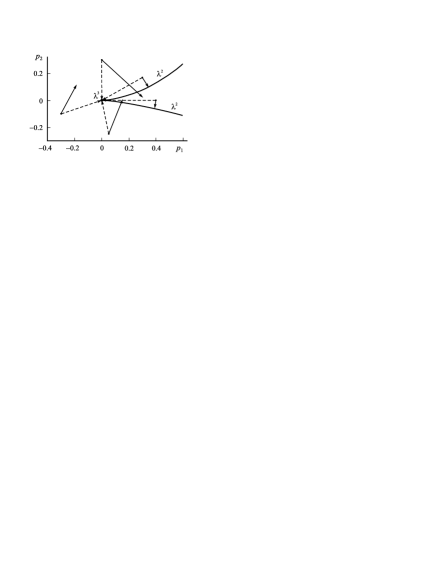
Figure 3: One-step approximations of the nearest points of the strata $\lambda^{2}$ (solid arrows) and $\lambda^{3}$ (dashed arrows) near the cusp singularity.

For the backward error analysis of numerical eigenvalue problems based on the study of the pseudo-spectrum we refer to [37]. We note that the classical numerical eigenvalue problem is ill-conditioned in the presence of multiple eigenvalues. The reason for that is the nonsmoothness of eigenvalues at multiple points giving rise to singular perturbation terms of order $\varepsilon^{1/d}$, where $d$ is the size of Jordan block [35]. On the contrary, in our problem we deal with the regular smooth objects: the strata $\lambda^{d}$ and the versal deformation $\mathbf{B}(\mathbf{p})$.

7 Approximations based on diagonal decomposition

In this section we consider approximations derived by using the diagonal decomposition of $\mathbf{A}_{0}$. The diagonal decomposition is known to be ill-conditioned for nearly defective matrices. However, this way is easy to implement, while the very high accuracy may be not necessary. According to bifurcation theory for eigenvalues [35], the accuracy of the results based on the diagonal decomposition will be of order $\varepsilon^{1/d}$, where $\varepsilon$ is the arithmetics precision. Another reason is theoretical. Bifurcation theory describes the collapse of a Jordan block into simple eigenvalues [32, 35, 38]. Our approximations based on the diagonal decomposition solve the inverse problem: using simple (perturbed) eigenvalues and corresponding eigenvectors, we approximate the stratum $\lambda^{d}$ at which these eigenvalues coalesce.

Let us assume that the matrix $\mathbf{A}_{0}$ is diagonalizable (its eigenvalues $\lambda_{1},\ldots,\lambda_{m}$ are distinct). The right and left eigenvectors of $\mathbf{A}_{0}$ are determined by the equations

$$\mathbf{A}_{0}\mathbf{x}_{i}=\lambda_{i}\mathbf{x}_{i},\quad\mathbf{y}_{i}^{*}\mathbf{A}_{0}=\lambda_{i}\mathbf{y}_{i}^{*},\quad\mathbf{y}_{i}^{*}\mathbf{x}_{i}=1$$ (7.1)

with the last equality being the normalization condition.

In Theorem 3.1 we take $\mathbf{S}={\rm diag}(\lambda_{1},\ldots,\lambda_{d})=\mathbf{Y}^{*}\mathbf{A}_{0}\mathbf{X}$, $\mathbf{X}=[\mathbf{x}_{1},\ldots,\mathbf{x}_{d}]$, and $\mathbf{Y}=[\mathbf{y}_{1},\ldots,\mathbf{y}_{d}]$, where $\lambda_{1},\ldots,\lambda_{d}$ are the eigenvalues coalescing at $\mathbf{p}\in\lambda^{d}$. In this case expressions (3.5) take the form

$$\begin{array}[]{l}\displaystyle\frac{\partial q_{1}}{\partial p_{j}}=\frac{1}{d}\sum_{i=1}^{d}\mathbf{y}_{i}^{*}\frac{\partial\mathbf{A}}{\partial p_{j}}\mathbf{x}_{i},\\[15.0pt] \displaystyle\frac{\partial q_{i}}{\partial p_{j}}=\sum_{i=1}^{d}(\lambda_{i}-q_{1}(\mathbf{p}_{0}))^{i-1}\mathbf{y}_{i}^{*}\frac{\partial\mathbf{A}}{\partial p_{j}}\mathbf{x}_{i}-\mathrm{trace}(\mathbf{C}^{i-1})\frac{\partial q_{1}}{\partial p_{j}}-\sum_{k=2}^{i-1}\mathrm{trace}(\mathbf{C}^{i-1}\mathbf{E}_{k1})\frac{\partial q_{k}}{\partial p_{j}},\\[15.0pt] \qquad i=2,\ldots,d;\ j=1,\ldots,n.\end{array}$$ (7.2)

The interesting feature of these expressions is that they depend only on the simple eigenvalues $\lambda_{1},\ldots,\lambda_{d}$ and their derivatives with respect to parameters at $\mathbf{p}_{0}$ [35]:

$$\frac{\partial\lambda_{i}}{\partial p_{j}}=\mathbf{y}_{i}^{*}\frac{\partial\mathbf{A}}{\partial p_{j}}\mathbf{x}_{i},\quad i=1,\ldots,d.$$ (7.3)

For example, for $d=2$ we obtain the first-order approximation of the surface $\lambda^{2}$ in the form of one linear equation

$$\delta^{2}+\delta\sum_{j=1}^{n}\left(\mathbf{y}_{2}^{*}\frac{\partial\mathbf{A}}{\partial p_{j}}\mathbf{x}_{2}-\mathbf{y}_{1}^{*}\frac{\partial\mathbf{A}}{\partial p_{j}}\mathbf{x}_{1}\right)(p_{j}-p_{j}^{0})=0,\quad\delta=\frac{\lambda_{2}-\lambda_{1}}{2}.$$ (7.4)

Let us introduce the gradient vectors $\nabla\lambda_{i}=(\partial\lambda_{i}/\partial p_{1},\ldots,\partial\lambda_{i}/\partial p_{n})$, $i=1,2$, with the derivatives $\partial\lambda_{i}/\partial p_{j}$ given by expression (7.3). Then the solution of (7.4) approximating the vector $\mathbf{p}\in\lambda^{2}$ nearest to $\mathbf{p}_{0}$ is found as

$$\mathbf{p}=\mathbf{p}_{0}-\frac{\overline{\nabla\lambda_{2}}-\overline{\nabla\lambda_{1}}}{\|\nabla\lambda_{2}-\nabla\lambda_{1}\|^{2}}\,\delta.$$ (7.5)

It is instructive to compare this result with the first-order approximation of the nearest $\mathbf{p}\in\lambda^{2}$, if we consider $\lambda_{1}$ and $\lambda_{2}$ as smooth functions

$$\lambda_{i}(\mathbf{p})=\lambda_{i}+\sum_{j=1}^{n}\frac{\partial\lambda_{i}}{\partial p_{j}}\,(p_{j}-p_{j}^{0})+O(\|\mathbf{p}-\mathbf{p}_{0}\|^{2}),\quad i=1,2.$$ (7.6)

Using (7.6) in the equation $\lambda_{1}(\mathbf{p})=\lambda_{2}(\mathbf{p})$ and neglecting higher order terms, we find

$$\sum_{j=1}^{n}\left(\frac{\partial\lambda_{2}}{\partial p_{j}}-\frac{\partial\lambda_{1}}{\partial p_{j}}\right)(p_{j}-p_{j}^{0})=\lambda_{1}-\lambda_{2},$$ (7.7)

which yields the nearest $\mathbf{p}$ as

$$\mathbf{p}=\mathbf{p}_{0}-\frac{\overline{\nabla\lambda_{2}}-\overline{\nabla\lambda_{1}}}{\|\nabla\lambda_{2}-\nabla\lambda_{1}\|^{2}}\,2\delta.$$ (7.8)

Comparing (7.8) with (7.5), we see that considering simple eigenvalues as smooth functions, we find the correct direction to the nearest point $\mathbf{p}\in\lambda^{2}$, but make a mistake in the distance to the stratum $\lambda^{2}$ overestimating it exactly twice. This is the consequence of the bifurcation taking place at $\mathbf{p}\in\lambda^{2}$ and resulting in $O(\|\mathbf{p}-\mathbf{p}_{0}\|^{1/2})$ perturbation of eigenvalues and eigenvectors [32, 35, 38].

8 Conclusion

In the paper, we developed Newton’s method for finding multiple eigenvalues with one Jordan block in multiparameter matrix families. The method provides the nearest parameter vector with a matrix possessing an eigenvalue of given multiplicity. It also gives the generalized eigenvectors and describes the local structure (tangent plane) of the stratum $\lambda^{d}$. The motivation of the problem comes from applications, where matrices describe behavior of a system depending on several parameters.

The whole matrix space has been considered as a particular case, when all entries of a matrix are independent parameters. Then the method provides an algorithm for solving the Wilkinson problem of finding the distance to the nearest degenerate matrix.

Only multiple eigenvalues with one Jordan block have been studied. Note that the versal deformation is not universal for multiple eigenvalues with several Jordan blocks (the functions $q_{1}(\mathbf{p}),\ldots,q_{d}(\mathbf{p})$ are not uniquely determined by the matrix family) [3, 4]. This requires modification of the method. Analysis of this case is the topic for further investigation.

9 Appendix

9.1 Proof of Theorem 3.1

Taking equation (2.5) at $\mathbf{p}_{0}$, we obtain

$$\mathbf{A}_{0}\mathbf{U}_{0}=\mathbf{U}_{0}\mathbf{B}_{0},$$ (9.1)

where $\mathbf{U}_{0}=\mathbf{U}(\mathbf{p}_{0})$ and $\mathbf{B}_{0}=\mathbf{B}(\mathbf{p}_{0})$. Comparing (9.1) with (3.1), we find that the matrix $\mathbf{B}_{0}$ is equivalent up to a change of basis to the matrix $\mathbf{S}$. Then the equality (3.3) is obtained by equating the traces of the matrices $\mathbf{B}_{0}$ and $\mathbf{S}$, where $\mathbf{B}_{0}$ has the form (2.5). Similarly, the equality (3.4) is obtained by equating the characteristic equations of the matrices $\mathbf{B}_{0}-q_{1}(\mathbf{p}_{0})\mathbf{I}$ and $\mathbf{S}-q_{1}(\mathbf{p}_{0})\mathbf{I}$.

The columns of the matrices $\mathbf{X}$ and $\mathbf{U}_{0}$ span the same invariant subspace of $\mathbf{A}_{0}$. Hence, the matrices $\mathbf{X}$ and $\mathbf{U}_{0}$ are related by the expression

$$\mathbf{U}_{0}=\mathbf{X}\mathbf{F},$$ (9.2)

for some nonsingular $d\times d$ matrix $\mathbf{F}$. Using (3.1) and (9.2) in (9.1), we find the relation

$$\mathbf{S}\mathbf{F}=\mathbf{F}\mathbf{B}_{0}.$$ (9.3)

Taking derivative of equation (2.5) with respect to parameter $p_{j}$ at $\mathbf{p}_{0}$, we obtain

$$\mathbf{A}_{0}\frac{\partial\mathbf{U}}{\partial p_{j}}-\frac{\partial\mathbf{U}}{\partial p_{j}}\mathbf{B}_{0}=\mathbf{U}_{0}\frac{\partial\mathbf{B}}{\partial p_{j}}-\frac{\partial\mathbf{A}}{\partial p_{j}}\mathbf{U}_{0}.$$ (9.4)

Let us multiply both sides of (9.4) by the matrix $\mathbf{F}^{-1}(\mathbf{S}-q_{1}(\mathbf{p}_{0})\mathbf{I})^{i-1}\mathbf{Y}^{*}$ and take the trace. Using expressions (3.1), (9.3), and the property $\mathrm{trace}(\mathbf{A}\mathbf{B})=\mathrm{trace}(\mathbf{B}\mathbf{A})$, it is straightforward to check that the left-hand side vanishes and we obtain the equation

$$0=\mathrm{trace}\left(\Big{(}\mathbf{U}_{0}\frac{\partial\mathbf{B}}{\partial p_{j}}-\frac{\partial\mathbf{A}}{\partial p_{j}}\mathbf{U}_{0}\Big{)}\mathbf{F}^{-1}(\mathbf{S}-q_{1}(\mathbf{p}_{0})\mathbf{I})^{i-1}\mathbf{Y}^{*}\right).$$ (9.5)

Substituting (9.2) into (9.5) and using equalities (3.1), (9.3), and $\mathbf{B}_{0}=q_{1}(\mathbf{p}_{0})\mathbf{I}+\mathbf{C}$, we find

$$\mathrm{trace}\left(\mathbf{C}^{i-1}\frac{\partial\mathbf{B}}{\partial p_{j}}\right)-\mathrm{trace}\left((\mathbf{S}-q_{1}(\mathbf{p}_{0})\mathbf{I})^{i-1}\mathbf{Y}^{*}\frac{\partial\mathbf{A}}{\partial p_{j}}\mathbf{X}\right)=0.$$ (9.6)

Using (2.5), (3.6) and taking into account that $\mathrm{trace}(\mathbf{C}^{i-1}\mathbf{E}_{k1})=0$ for $k>i$, we obtain

$$\mathrm{trace}(\mathbf{C}^{i-1})\frac{\partial q_{1}}{\partial p_{j}}+\sum_{k=2}^{i}\mathrm{trace}(\mathbf{C}^{i-1}\mathbf{E}_{k1})\frac{\partial q_{k}}{\partial p_{j}}=\mathrm{trace}\left((\mathbf{S}-q_{1}(\mathbf{p}_{0})\mathbf{I})^{i-1}\mathbf{Y}^{*}\frac{\partial\mathbf{A}}{\partial p_{j}}\mathbf{X}\right).$$ (9.7)

Taking equation (9.7) for $i=1,\ldots,d$ and using the equality $\mathrm{trace}(\mathbf{C}^{i-1}\mathbf{E}_{i1})=1$, we get the recurrent procedure (3.5) for calculation of derivatives of $q_{1}(\mathbf{p}),\ldots,q_{d}(\mathbf{p})$ at $\mathbf{p}_{0}$.

9.2 Proof of Theorem 3.2

At $\mathbf{p}_{0}\in\lambda^{d}$, we have $q_{2}(\mathbf{p}_{0})=\cdots=q_{d}(\mathbf{p}_{0})=0$. From (2.5) it follows that $\mathbf{B}_{0}=\mathbf{J}_{\lambda}$ is the Jordan block with the eigenvalue $\lambda=q_{1}(\mathbf{p}_{0})=\mathrm{trace}\,\mathbf{S}/d$. By using (3.1), one can check that the vectors (3.10) satisfy the Jordan chain equations (2.1) for any vector $\mathbf{k}$. Equations (3.11) provide the way of choosing a particular value of the vector $\mathbf{k}$.

Since $\mathbf{B}_{0}=\mathbf{J}_{\lambda}$, the versal deformation equation (2.5) becomes the Jordan chain equation (2.2) at $\mathbf{p}_{0}\in\lambda^{d}$. Hence, the columns of the matrix $\mathbf{U}_{0}$ are the generalized eigenvectors. Since the function $q_{1}(\mathbf{p})$ and the matrix $\mathbf{U}(\mathbf{p})$ smoothly depend on parameters, the accuracy of the multiple eigenvalue and generalized eigenvectors has the same order as the accuracy of $\mathbf{p}_{0}\in\lambda^{d}$.

References

- [1] E. Anderson, Z. Bai, C. Bischof, L. S. Blackford, J. Demmel, J. Dongarra, J. Du Croz, A. Greenbaum, S. Hammarling, A. McKenney and D. Sorensen. LAPACK Users’ Guide (3rd edn). SIAM: Philadelphia, 1999.
- [2] I. E. Antoniou, M. Gadella, E. Hernandez, A. Jauregui, Yu. Melnikov, A. Mondragon and G. P. Pronko. Gamow vectors for barrier wells. Chaos, Solitons and Fractals 2001; 12:2719–2736.
- [3] V. I. Arnold. Matrices depending on parameters. Russian Math. Surveys 1971; 26(2):29–43.
- [4] V. I. Arnold. Geometrical Methods in the Theory of Ordinary Differential Equations. Springer-Verlag: New York-Berlin, 1983.
- [5] M. V. Berry and M. R. Dennis. The optical singularities of birefringent dichroic chiral crystals. Proc. Roy. Soc. Lond. A 2003; 459:1261–1292.
- [6] J. V. Burke, A. S. Lewis and M. L. Overton. Optimal stability and eigenvalue multiplicity. Found. Comput. Math. 2001; 1(2):205–225.
- [7] J. W. Demmel. Computing stable eigendecompositions of matrices. Linear Algebra Appl. 1986; 79:163–193.
- [8] I. Dobson, J. Zhang, S. Greene, H. Engdahl and P. W. Sauer. Is strong modal resonance a precursor to power system oscillations? IEEE Transactions On Circuits And Systems I: Fundamental Theory And Applications 2001; 48:340–349.
- [9] A. Edelman, E. Elmroth and B. Kågström. A geometric approach to perturbation theory of matrices and matrix pencils. I. Versal deformations. SIAM J. Matrix Anal. Appl. 1997; 18(3):653–692.
- [10] A. Edelman and Y. Ma. Staircase failures explained by orthogonal versal forms. SIAM J. Matrix Anal. Appl. 2000; 21(3):1004–1025.
- [11] E. Elmroth, P. Johansson and B. Kågström. Bounds for the distance between nearby Jordan and Kronecker structures in closure hierarchy. In Numerical Methods and Algorithms XIV, Zapiski Nauchnykh Seminarov (Notes of Scientific Seminars of POMI) 2000; 268:24–48.
- [12] E. Elmroth, P. Johansson and B. Kågström. Computation and presentation of graphs displaying closure hierarchies of Jordan and Kronecker structures. Numerical Linear Algebra with Applications 2001; 8(6–7):381–399.
- [13] T. F. Fairgrieve. The application of singularity theory to the computation of Jordan canonical form. M.Sc. Thesis, Department of Computer Science, University of Toronto, 1986.
- [14] F. R. Gantmacher. The Theory of Matrices. AMS Chelsea Publishing: Providence, RI, 1998.
- [15] G. H. Golub and C. F. Van Loan. Matrix computations (3rd edn). Johns Hopkins University Press: Baltimore, 1996.
- [16] G. H. Golub and J. H. Wilkinson. Ill-conditioned eigensystems and the computation of the Jordan canonical form. SIAM Rev. 1976; 18(4):578–619.
- [17] W. D. Heiss. Exceptional points – their universal occurrence and their physical significance. Czech. J. Phys. 2004; 54:1091–1099.
- [18] B. Kågström and A. Ruhe. An algorithm for numerical computation of the Jordan normal form of a complex matrix. ACM Trans. Math. Software 1980; 6(3):398–419.
- [19] B. Kågström and A. Ruhe. ALGORITHM 560: JNF, An algorithm for numerical computation of the Jordan normal form of a complex matrix [F2]. ACM Trans. Math. Software 1980; 6(3):437–443.
- [20] O. N. Kirillov. A theory of the destabilization paradox in non-conservative systems. Acta Mechanica 2005; to appear.
- [21] O. N. Kirillov and A. P. Seyranian. Optimization of stability of a flexible missile under follower thrust, in Proceedings of the 7th AIAA/USAF/NASA/ISSMO Symposium on Multidisciplinary Analysis and Optimization, St. Louis, MO, USA, 1998. AIAA Paper #98-4969. P. 2063–2073.
- [22] H. J. Korsch and S. Mossmann. Stark resonances for a double quantum well: crossing scenarios, exceptional points and geometric phases. J. Phys. A: Math. Gen. 2003; 36:2139–2153.
- [23] V. Kublanovskaya. On a method of solving the complete eigenvalue problem of a degenerate matrix. USSR Comput. Math. Math. Phys. 1966; 6(4):1–14.
- [24] O. Latinne, N. J. Kylstra, M. D orr, J. Purvis, M. Terao-Dunseath, C. J. Jochain, P. G. Burke and C. J. Noble. Laser-induced degeneracies involving autoionizing states in complex atoms. Phys. Rev. Lett. 1995; 74:46–49.
- [25] A. S. Lewis and M. L. Overton. Eigenvalue optimization. Acta Numerica 1996; 5:149–190.
- [26] R. A. Lippert and A. Edelman. The computation and sensitivity of double eigenvalues. In Advances in Computational Mathematics. Lecture Notes in Pure and Applied Mathematics. Vol. 202, Z. Chen, Y. Li, C. A. Micchelli, and Y. Xi, (eds). Dekker: New York, 1999; 353-393.
- [27] A. A. Mailybaev. Transformation of families of matrices to normal forms and its application to stability theory. SIAM J. Matrix Anal. Appl. 2000; 21(2):396–417.
- [28] A. A. Mailybaev. Transformation to versal deformations of matrices. Linear Algebra Appl. 2001; 337(1–3):87–108.
- [29] A. A. Mailybaev and A. P. Seiranyan. On the domains of stability of Hamiltonian systems. J. Appl. Math. Mech. 1999; 63(4):545–555.
- [30] A. A. Mailybaev and A. P. Seyranian. On singularities of a boundary of the stability domain. SIAM J. Matrix Anal. Appl. 2000; 21(1):106–128.
- [31] MATLAB routines for computation of multiple eigenvalues and generalized eigenvectors for matrices dependent on parameters, on request by e-mail: mailybaev@imec.msu.ru
- [32] J. Moro, J. V. Burke and M. L. Overton. On the Lidskii-Vishik-Lyusternik perturbation theory for eigenvalues of matrices with arbitrary Jordan structure. SIAM J. Matrix Anal. Appl. 1997; 18(4):793–817.
- [33] A. Ruhe. An algorithm for numerical determination of the structure of a general matrix. BIT 1970; 10:196–216.
- [34] A. P. Seyranian, O. N. Kirillov and A. A. Mailybaev. Coupling of eigenvalues of complex matrices at diabolic and exceptional points. J. Phys. A: Math. Gen. 2005; 38, to appear.
- [35] A. P. Seyranian and A. A. Mailybaev. Multiparameter Stability Theory with Mechanical Applications. World Scientific: Singapore, 2003.
- [36] A. P. Seyranian and P. Pedersen. On interaction of eigenvalue branches in non-conservative multi-parameter problems. In Dynamics and Vibration of Time-Varying Systems and Structures: Conf. on Mech. Vibrat. and Noise. ASME: New York, 1993; 19–31.
- [37] E. Traviesas. Sur le déploiement du champ spectral d’une matrice. Ph.D. dissertation, Universite Toulouse I, France, 2000.
- [38] M. I. Vishik and L. A. Lyusternik. The solution of some perturbation problems for matrices and selfadjoint or non-selfadjoint differential equations I. Russian Math. Surveys 1960; 15:1–74.
- [39] J. H. Wilkinson. The Algebraic Eigenvalue Problem. Clarendon Press: Oxford, 1965.
- [40] J. H. Wilkinson. Sensitivity of eigenvalues. Util. Math. 1984; 25:5–76.
- [41] J. H. Wilkinson. Sensitivity of eigenvalues II. Util. Math. 1986; 30:243–286.