Remarks on $\mathcal{PT}$-pseudo-norm in $\mathcal{PT}$-symmetric quantum mechanics

Abstract

This paper presents an underlying analytical relationship between the $\mathcal{PT}$-pseudo-norm associated with the $\mathcal{PT}$-symmetric Hamiltonian $H=p^{2}+V(q)$ and the Stokes multiplier of the differential equation corresponding to this Hamiltonian. We show that the sign alternation of $\mathcal{PT}$-pseudo-norm, which has been observed as a generic feature of the $\mathcal{PT}$-inner product, is essentially controlled by the derivative of Stokes multiplier with respect to eigenparameter.

Keywords: Eigenvalue problems, Stokes multipliers, $\mathcal{PT}$-symmetry, entire functions.

PACS : 03.65.Ge, 11.30.Er, 03.65.Ca

1. Introduction

Since the late 1990’s, the notion of $\mathcal{PT}$-symmetric Hamiltonians in quantum physics is addressed in many works after its first appearance in a publication of Bender and Boettcher [6] concerning a conjecture of Bessis and Zinn-Justin.

By dropping the requirement of Hermiticity but of course keeping the invariance by the Lorentz group, one opens on a significantly larger class of Hamiltonians satisfying a weaker hypothesis, namely the $\mathcal{PT}$-invariance. This more flexible condition amounts to the commutability of the Hamiltonian $H$ and the composite operator $\mathcal{PT}$ whose components consist of one linear operator $\mathcal{P}$ (for parity) and another anti-linear $\mathcal{T}$ (for time-reversal).

It has been showed that, despite the lack of Hermiticity, many $\mathcal{PT}$-symmetric Hamiltonians still have a whole real and bounded from below discrete spectrum (see [4, 8, 11, 15, 17, 19, 23, 31]). However, a controversy has merged among researchers due to the fact that the space of states may be no longer a Hilbert space, at variance with traditional quantum mechanics.

Recently, many studies have been devoted to the establishment of a conventional mathematical structure for $\mathcal{PT}$-symmetry quantum mechanics (see [2, 3, 27, 28]). One of the most important considerations is to equip the space of states associated with a given Hamiltonian with a certain inner product, so suitably that the norm induced by this inner product is positive definite.

For Hermitian Hamiltonians on the real axis $\mathbb{R}$, such a space is normally known as the Hilbert space $L^{2}(\mathbb{R})$, whose inner product is nothing but the usual one. The norm induced from this actually positive definite inner product is interpreted as a probability density in the space of states.

Such an ideal model seems to be no longer available whenever the Hamiltonians are non-Hermitian. However, the specialists in the field have recently succeeded in constructing a consistent physical theory for unbroken $\mathcal{PT}$-symmetric Hamiltonians. The most essential aspect in their investigations is the appearance of a linear “charge” operator $\mathcal{C}$ whose action enables the so-called $\mathcal{PT}$-pseudo-norm to switch its sign in a suitable way, so that the induced $\mathcal{CPT}$-norm is now positive definite.

This operator $\mathcal{C}$ is nowdays a central subject of interest. Recently, in an attempt to formulate $\mathcal{PT}$-symmetric quantum theories, Bender et al have obtained many significant results through explicit calculation of the operator $\mathcal{C}$ for some special $\mathcal{PT}$-symmetric Hamiltonians (see [2, 3, 5]). As a rule, the construction relies on the observation of a so-called quasi-parity quantum number [1, 24, 37], so that the $\mathcal{PT}$-pseudo-norm exhibits a generic sign alternation, upon the eigenstates of Hamiltonians.

This paper, which is motivated by these observations, aims mainly to justify the indefiniteness of the $\mathcal{PT}$-inner product for a class of unbroken $\mathcal{PT}$-symmetric Hamiltonians. By using some classical results on Stokes multipliers (see [32], ch. $5,6$), whose zeros are exactly the eigenvalues of the considered Hamiltonians, we show an analytical relation between the $\mathcal{PT}$-pseudo-norm and the derivative with respect to the eigenparameter of one of these Stokes multipliers, from which the sign alternation occurs as a natural consequence.

This paper is organized as follows. In section 2 we recall some simple notions and facts on the Sturm-Liouville eigenvalue problem associated with a class of complex Hamiltonians. A strong connection between our problem and Sibuya’s theory on linear differential equations is formulated for our next purposes. Section 3 contains our main results which allow to establish a relationship between the $\mathcal{PT}$-pseudo-norm and the derivative in the eigenparameter of a convenient Stokes multiplier. This gives a clear explanation for the indefiniteness of the $\mathcal{PT}$-pseudo-norm, thus justifying what has been observed in various works (e.g., [2]). Finally, in the conclusion we suggest some further considerations and discuss a degenerate case, where the $\mathcal{PT}$-symmetry may be spontaneously broken by the vanishing of the $\mathcal{PT}$-pseudo-norm at some degenerate states.

2. Sturm-Liouville eigenvalue problem associated to a Hamiltonian

We consider a non-Hermitian Hamiltonian

$$H=p^{2}+V(q)$$ (1)

where $p$ stands for the operator $-i\frac{d}{dq}$ and

$$V(q):=-[(iq)^{m}+a_{1}(iq)^{m-1}+\cdots+a_{m-1}(iq)+a_{m}]$$ (2)

is a polynomial of degree $m$ in the variable $iq$ with real coefficients $a_{j}\in\mathbb{R}$.

These assumptions induce that the complex-valued potential function $V(q)$ satisfies the following relation,

$$\overline{V(-\overline{q})}=V(q)$$ (3)

(where $\overline{q}$ stands for the complex conjugate of $q$), which is broadly known as the $\mathcal{PT}$-symmetry, or more geometrically as the invariance property of $V(q)$ under the real conjugation.

Recall that, as usual, the combination $\mathcal{PT}$ stands for the composite operator of $\mathcal{P}$ (parity operator) and $\mathcal{T}$ (time-reversal operator) whose actions on the $(p,q)$-space are generally determined as follows:

$$\mathcal{P}:\left\{\begin{array}[]{l}q\mapsto-q\\ p\mapsto-p\end{array}\right.\quad\rm{and}\quad\mathcal{T}:\left\{\begin{array}[]{l}q\mapsto\overline{q}\\ p\mapsto-\overline{p}\end{array}\right.$$

By definition, $\mathcal{PT}(=\mathcal{TP})$ is not a linear but an anti-linear operator. Its action on a wave function $\phi(q)$ is simply given by

$$\mathcal{PT}\phi(q)=\overline{\phi(-\overline{q})}.$$ (4)

Consequently, a function $\phi(q)$ is called $\mathcal{PT}$-symmetric if it remains unchanged under the action of the operator $\mathcal{PT}$ in (4). It is obvious that the Hamiltonian $H$ in (1) is $\mathcal{PT}$-symmetric, i.e.

$$\mathcal{PT}H=H\mathcal{PT}$$ (5)

provided that $V(q)$ is $\mathcal{PT}$-symmetric. And this is the case when all coefficients $a_{j}$ in (2) are real.

$\mathcal{PT}$-inner product and $\mathcal{PT}$-pseudo-norm.

In the sequel, we shall determine a space of functions on which the action of our given Hamiltonian is meaningful. We note that the usual set of functions considered for most (Hermitian) Hamiltonians on the real line is $L^{2}(\mathbb{R})$, in relation to its useful Hilbert space structure. In the context of non-Hermitian Hamiltonians, defining such a space with an appropriate algebraic structure has not been yet completely settled in general.

Consider the Hamiltonian $H$ in (1) with the assumption that all $a_{j}$ in (2) are real, so that $H$ is $\mathcal{PT}$-symmetric. For a fixed $m\in\mathbb{N}$, $m\geq 2$, we denote by $\mathfrak{H}$ the complex vector space of all entire functions $f(q)$ which are exponentially vanishing at infinity in both of the two open sectors

$$\begin{array}[]{lll}&&S_{l}:=\left\{\big{|}\arg(X)+\frac{\pi}{2}+\frac{2\pi}{m+2}\big{|}<\frac{\pi}{m+2}\right\}\\ \vspace{3mm}{\rm and}&&S_{r}:=\left\{\big{|}\arg(X)+\frac{\pi}{2}-\frac{2\pi}{m+2}\big{|}<\frac{\pi}{m+2}\right\}\\ \end{array}$$ (6)

This space $\mathfrak{H}$ can be considered as a vector subspace of the space of square integrable functions in both the two neighborhoods of infinity ${S_{l}}$ and ${S_{r}}$. By virtue of the involution of $\mathcal{PT}$ and the definition of $\mathfrak{H}$, we have immediately

$$\mathcal{PT}(\mathfrak{H})=\mathfrak{H}.$$ (7)

The following statement, which can be checked directly, asserts the symmetry of the discrete spectrum of a $\mathcal{PT}$-symmetric Hamiltonian.

Proposition 1.

Let $\mathfrak{G}$ be a certain vector space of functions satisfying $\mathcal{PT}(\mathfrak{G})\subset\mathfrak{G}$. Then the set of eigenvalues of a $\mathcal{PT}$-symmetry Hamiltonian $H$ acting on $\mathfrak{G}$ is invariant under complex conjugation.

We are going to introduce a space in which each eigenfunction of the non-Hermitian Hamiltonian $H$ is associated with a real number, usually (but a bit abusively) called its $\mathcal{PT}$-pseudo-norm.

Instead of considering the real axis, as it is the case for the usual norm in $L^{2}(\mathbb{R})$, a slightly different curve will be involved in order to be consistent with our goals. Consider an endless curve $\gamma$ starting from infinity in the sector $S_{l}$ and ending also at infinity but in the different sector $S_{r}$. Note that for a given function $h(q)\in\mathfrak{H}$, which is thus holomorphic and integrable at infinity in ${S_{l}}\cup{S_{r}}$, the value of the integral $\displaystyle\int_{\gamma}h(q)dq$ remains unchanged when $\gamma$ is deformed continuously such that both of its endpoints still lie in $S_{l}$ and $S_{r}$ respectively.

For the sake of simplicity, we shall take $\gamma$ to be symmetric so that, up to its orientation, the mapping $q\mapsto-\overline{q}$ of the complex plane $\mathbb{C}$, which is nothing but the mirror symmetry with respect to the imaginary axis, leaves $\gamma$ invariant. Precisely, it will be convenient to define $\gamma$ by:

$$\gamma:=\gamma_{r}-\gamma_{l},$$ (8)

where $\gamma_{r}$ and $\gamma_{l}$ (drawn on Fig.1) are respectively the rays oriented from the origin to infinity such that

$$\gamma_{l}=\Big{\{}q\in\mathbb{C}/\arg(q)=-\frac{\pi}{2}-\frac{2\pi}{m+2}\Big{\}},\hskip 14.22636pt\gamma_{r}=\Big{\{}q\in\mathbb{C}/\arg(q)=-\frac{\pi}{2}+\frac{2\pi}{m+2}\Big{\}}.$$

We now introduce a sesquilinear form on $\mathfrak{H}$ as follows. For $f,g\in\mathfrak{H}$, we define

$$\ll f,g\gg_{\gamma}\,:=\int_{\gamma}f(q)\mathcal{PT}g(q)dq=\int_{\gamma}f(q)\overline{g(-\overline{q})}dq$$ (9)

By changing the variable of integration $z=-\overline{q}$, one easily checks that for every $f,g\in\mathfrak{H}$,

$$\ll f,g\gg_{\gamma}\,=\overline{\ll g,f\gg}_{\gamma}.$$ (10)

This means that $\ll f,g\gg_{\gamma}$ realizes a Hermitian sesquilinear form on $\mathfrak{H}$.

We naturally define the mapping $\|\cdot\|_{\mathcal{PT}}^{2}:\mathfrak{H}\rightarrow\mathbb{R}$ induced by (10):

$$\|f\|_{\mathcal{PT}}^{2}:=\,\ll f,f\gg_{\gamma}$$ (11)

Here, it is necessary to emphasize that the Hermitian sesquilinear form $\ll.,.\gg_{\gamma}$ has no reason to be positive definite. In particular, $\|f\|_{\mathcal{PT}}^{2}$ can be zero even if $f\neq 0$. Hence, it is deservedly called $\mathcal{PT}$-pseudo-norm, while the form $\ll.,.\gg_{\gamma}$ will be called $\mathcal{PT}$-inner product.

Proposition 2.

The $\mathcal{PT}$-symmetric Hamiltonian $H$ is symmetric under the $\mathcal{PT}$-inner product:

$$\ll H\phi,\psi\gg_{\gamma}\,=\ll\phi,H\psi\gg_{\gamma}\,\qquad\qquad\forall\,\phi,\psi\in\mathfrak{H}.$$

Proof.

We note that if $\phi$ belongs to $\mathfrak{H}$, then $H\phi\in\mathfrak{H}$ also. Now by definition we have

$$\ll H\phi,\psi\gg_{\gamma}\,=\int_{\gamma}H\phi\mathcal{PT}\psi dq=\int_{\gamma}(-\phi^{\prime\prime}+V(q)\phi)\mathcal{PT}\psi dq.$$

Integrating the right-hand side by parts twice yields

$$\begin{array}[]{ll}\displaystyle\ll H\phi,\psi\gg_{\gamma}&\displaystyle=\int_{\gamma}\phi\big{(}-(\mathcal{PT}\psi)^{\prime\prime}+V(q)\mathcal{PT}\psi\big{)}dq\\ \vspace{2mm}&\displaystyle=\int_{\gamma}\phi H\mathcal{PT}\psi dq=\int_{\gamma}\phi\mathcal{PT}H\psi dq=\ll\phi,H\psi\gg_{\gamma}.\\ \end{array}$$

This completes the proof. ∎

This proposition induces the following two direct consequences.

Corollary 2.1.

Two eigenfunctions corresponding to distinguish real eigenvalues are orthogonal with respect to $\ll\cdot,\cdot\gg_{\gamma}$.

Corollary 2.2.

If $\phi_{E}$ is an eigenfunction corresponding to a complex eigenvalue $E$ then $\|\phi_{E}\|_{\mathcal{PT}}^{2}=0$.

Stokes multipliers

In what follows we briefly recall some important results of Sibuya [32] on complexe second-order linear differential equations. We consider in the complex plane the following equation

$$-\Phi^{\prime\prime}(X)+W(X)\Phi(X)=0$$ (12)

where $W(X)=X^{m}+a_{1}X^{m-1}+\cdots+a_{m}$ is a monic polynomial function of degree $m\in\mathbb{N}$, with coefficients $a_{1},a_{2},\ldots,a_{m}\in\mathbb{C}$.

The following theorem, which is due to Sibuya, asserts the existence and uniqueness of a solution characterized by its asymptotic behavior at infinity.

Theorem 3.

Equation (12) admits a unique solution $\Phi_{0}(X,a):=\Phi_{0}(X;a_{1},a_{2},\ldots,a_{m})$ such that:

1. $\Phi_{0}(X,a)$ is an entire function in $(X;a_{1},a_{2},\ldots,a_{m})$,

2. $\Phi_{0}(X,a)$ and its derivative $\Phi^{\prime}_{0}(X,a)$ admit the following asymptotic behaviors

   $$\Phi_{0}(X)\simeq X^{r_{m}}e^{-S(X,a)}\left[1+O(X^{-1/2})\right]$$ (13)

   $$\Phi^{\prime}_{0}(X)\simeq X^{\frac{m}{2}+r_{m}}e^{-S(X,a)}\left[-1+O(X^{-1/2})\right]$$ (14)

   when $X\rightarrow\infty$ in each sub-sector strictly contained in the sector

   $$\Sigma_{0}=\left\{|\arg(X)|<\frac{3\pi}{m+2}\right\}$$

   and the asymptotic regimes occur uniformly with respect to $a=(a_{1},a_{2},\ldots,a_{m})$ in any compact of $\mathbb{C}^{m}$.

In the above theorem $r_{m}$ and $S(X,a)$ can be determined explicitly from $W(X)$. As $X\rightarrow\infty$, one can write

$$\begin{array}[]{ll}\sqrt{W(X)}&=X^{\frac{m}{2}}\left\{1+a_{1}X^{-1}+\cdots+a_{m}X^{-m}\right\}^{1/2}\\ &=X^{\frac{m}{2}}\left\{1+\sum_{k=1}^{\infty}b_{k}(a)X^{-k}\right\}\\ \end{array}$$ (15)

where, obviously, $b_{k}(a)$ are quasi-homogeneous polynomials in $a_{1},\ldots,a_{m}$ with real coefficients.

By integrating term-by-term the series in the right-hand side, we get a primitive of $\sqrt{W(X)}$. The function $S(X,a)$ is associated to the “principal part” of this primitive

$$S(X,a)=\frac{2}{m+2}X^{\frac{m+2}{2}}+\cdots$$

that only contains terms with strictly positive powers of $X$. And $r_{m}=r_{m}(a)$ is given by

$$r_{m}(a)=\left\{\begin{array}[]{ll}-m/4&\rm{for}\;$m$\;\rm{odd}\\ -m/4-b_{1+m/2}(a)&\rm{for}\;$m$\;\rm{even}\\ \end{array}\right.$$ (16)

We should notice that for $m>2$, $r_{m}(a)$ does not depend on the last coefficient $a_{m}$ and if all $a_{j}$ (possibly except $a_{m}$) are equal to zero then $r_{m}=-m/4$.

We shall define other solutions of (12) by introducing a rotation of the complex plan. Let us denote

$$\omega:=\exp\left\{-\frac{i2\pi}{m+2}\right\}\,\,\rm{and}\,\,\omega_{k}(a):=(\omega^{k}a_{1},\omega^{2k}a_{2},\ldots,\omega^{km}a_{m});\,\,\,(k\in\mathbb{Z})$$

For each $k\in\mathbb{Z}$, we construct functions $\Phi_{k}(X;a)$ by setting

$$\Phi_{k}(X;a):=\Phi_{0}(\omega^{k}X;\omega_{k}(a)).$$ (17)

It is not difficult to check that $\Phi_{k}(X;a)$ are indeed solutions of (12) and exponentially vanishing at infinity in the corresponding sector

$$S_{k}:=\Big{\{}|\arg(X)-k\frac{2\pi}{m+2}|<\frac{\pi}{m+2}\Big{\}}.$$ (18)

The following lemma, which can be verified in a straightforward way (see [18, 32]), implies the linear independence of two consecutive solutions $\Phi_{k}$ and $\Phi_{k+1}$.

Lemma 4.

For any $k\in\mathbb{Z}$, the Wronskian of $\Phi_{k}$ and $\Phi_{k+1}$ is given by the formula

$${\sf Wr}(\Phi_{k},\Phi_{k+1})=2(-1)^{k}\omega^{-\frac{km}{2}+r_{m}(\omega_{k+1}(a))}$$ (19)

From this observation, together with classical results on the structure of solutions of linear differential equations, we can infer that $\{\Phi_{k},\Phi_{k+1}\}$ constitutes a basis for the vector space of the solutions of the equation (12). Therefore, every solution can be expressed as a linear combination of $\Phi_{k},\Phi_{k+1}$. In particular, for each $k\in\mathbb{Z}$, we have

$$\Phi_{k-1}=C_{k}(a)\Phi_{k}+\widetilde{C}_{k}(a)\Phi_{k+1}$$ (20)

The multipliers $C_{k}(a)$ and $\widetilde{C}_{k}(a)$ are called the Stokes multipliers of $\Phi_{k-1}$ with respect to $\Phi_{k}$ and $\Phi_{k+1}$. Further studies on these objects are addressed in [18, 29, 32]. By definition, it is evident that

$$C_{k}(a)=\frac{{\sf Wr}(\Phi_{k-1},\Phi_{k+1})}{{\sf Wr}(\Phi_{k},\Phi_{k+1})}\quad{\rm and}\quad\widetilde{C}_{k}(a)=\frac{{\sf Wr}(\Phi_{k-1},\Phi_{k})}{{\sf Wr}(\Phi_{k+1},\Phi_{k})}$$

Since $\Phi_{k}(X;a)$ are entire functions in $a$, it follows immediately from these equalities and Lemma 4 that $C_{k}(a)$ and $\widetilde{C}_{k}(a)$ are also entire functions in $a$. Furthermore, we also get an explicit expression for $\widetilde{C}_{k}(a)$

$${\widetilde{C}}_{k}(a)=\omega^{m+2r_{m}(\omega_{k}(a))}$$

We emphasize that $\widetilde{C}_{k}(a)$ is never vanishing. Thus, this coefficient can be reduced to 1 by a suitable renormalisation of the $\Phi_{k}$’s. For instance, when $k=0$, (20) reads

$$\Phi_{-1}=C_{0}(a)\Phi_{0}+\omega^{m+2r_{m}(a)}\Phi_{1}.$$ (21)

By setting

$$\begin{array}[]{ll}&Y_{1}:=\omega^{m/2+r_{m}(a)}\Phi_{1}=\omega^{m/2+r_{m}(a)}\Phi_{0}(\omega X;\omega(a))\\ \vspace{2mm}{\rm and}&Y_{-1}:=\omega^{-m/2-r_{m}(a)}\Phi_{-1}=\omega^{-m/2-r_{m}(a)}\Phi_{0}(\omega^{-1}X;\omega_{-1}(a))\ ,\\ \end{array}$$ (22)

we can write (21) under a slightly symmetric form,

$$Y_{-1}=C(a)Y_{0}+Y_{1},$$ (23)

where $Y_{0}$ stands for $\Phi_{0}$ and $C(a):=\omega^{-m/2-r_{m}(a)}C_{0}(a)$ is also called the Stokes multiplier of $Y_{-1}$ with respect to $Y_{0}$.

With these conventions, we get a very simple expression for the Wronskian of $Y_{0}$ and $Y_{1}$, namely:

$${\sf Wr}(Y_{0},Y_{1})=2.$$ (24)

Concerning the (sole) Stokes multiplier $C(a)$ in (23), which plays a very important role for our purposes, we have

Proposition 5.

For any $a\in\mathbb{C}^{m}$,

$$\overline{C(a)}+C(\overline{a})=0.$$ (25)

Proof.

By virtue of the quasi-homogeneity of the equation (12), we can see that $\overline{\Phi_{0}(\overline{X},\overline{a})}$ is also one of its solutions whose asymptotic behavior at $\infty$ in the sector $S_{0}$ is the same as $\Phi_{0}(X,a)$.

The uniqueness of the canonical solution in Theorem 3 implies immediately that

$$\overline{\Phi_{0}(X,a)}=\Phi_{0}(\overline{X},\overline{a})$$ (26)

Taking into account the above definitions of $Y_{-1}$ and $Y_{1}$, we can check without difficulty that

$$Y_{-1}(\overline{X},\overline{a})=\overline{Y_{1}(X,a)}$$ (27)

for any $X\in\mathbb{C}$ and any $a\in\mathbb{C}^{m}$.

Putting these relations in (23) leads the desired identity. ∎

Eigenvalues as zeros of the Stokes multiplier

We now consider the complex Sturm-Liouville eigenvalue problem associated with the Hamiltonian $H$ in (1):

$$\left\{\begin{array}[]{l}\displaystyle-\phi^{\prime\prime}(q)+V(q)\phi(q)=E\phi(q)\\ \\ \displaystyle\lim_{q\rightarrow-i\infty.e^{i\theta}}\phi(q)=0\quad{\rm and}\quad\lim_{q\rightarrow-i\infty.e^{-i\theta}}\phi(q)=0\\ \end{array}\right.$$ (28)

where $\theta:=\frac{2\pi}{m+2}$.

It is necessary to notice that the boundary condition ($\lim\phi(q)=0$) in (28) is equivalent to the fact that $\phi(q)$ is exponentially vanishing at infinity in both of the two sectors $S_{l}$ and $S_{r}$.

For our purposes, we prefer to consider the problem (28) in a new variable, introducing the rotation $q\mapsto X:=iq$. This transforms the differential equation in (28) into the following one:

$$-\Phi^{\prime\prime}(X)+(X^{m}+a_{1}X^{m-1}+\cdots+a_{m-1}X+E)\Phi(X)=0,$$ (29)

where $\Phi(X)$ stands for $\phi(q)$.

The boundary value conditions in (28) turn into the requirement that the solution $\Phi(X)$ vanishes exponentially in both of the two sectors $S_{-1}$ and $S_{1}$, which are defined in (18), see also Fig.1.

With the notations of the previous subsection and writing $C(a,E):=C(a_{1},\ldots,a_{m-1},E)$ for the Stokes multiplier, we have:

Lemma 6.

$E_{eigen}$ is an eigenvalue of the problem (28) if and only if $C(a,E_{eigen})=0$.

Proof.

Let $\phi_{eigen}(q)$ be an eigenfunction corresponding to the eigenvalue $E_{eigen}$. Then $Y_{eigen}(X):=\phi_{eigen}(-iX)$ solves (29) and vanishes exponentially at infinity in both of $S_{-1}$ and $S_{1}$ in the $X$-plane. This fact, together with the observation that $Y_{0}(X)$ growths exponentially in $S_{\pm 1}$, implies that $Y_{eigen}(X)$ is proportional to $Y_{\pm 1}(X)$ in $S_{\pm 1}$ respectively. By virtue of (23), this is only possible if $C(a,E_{eigen})=0$.

Conversely, if $E_{eigen}=E_{eigen}(a)$ is a zero of $C(a,E)$ then $Y_{eigen}(X):=Y_{-1}(X,E_{eigen})\equiv Y_{1}(X,E_{eigen})$ exponentially vanishes at $\infty$ in both of $S_{\pm 1}$. Replacing $X=iq$, we obtain a solution for (28). ∎

Remark 7.

We note that by construction, $C(a,E)$ is a non-constant entire function in both $a$ and $E$. For each fixed $a\in\mathbb{C}^{m-1}$, as an entire function of $E$, $C(a,E)$ has the order of $\frac{1}{2}+\frac{1}{m}$ (see [32]). Since the order is a non-integral positive number for $m>2$, $C(a,E)$ must have infinitely many zeros $E_{n}=E_{n}(a)$. By estimating the asymptotic behavior of $C(a,E)$ as $E\rightarrow\infty$, Sibuya proved that, except possibly for a finite number, these zeros are simple (i.e. the derivative $\frac{\partial}{\partial E}C(a,E)\neq 0$ at those points). Furthermore, the large zeros are known to be close to the positive real half-axis and satisfy the following estimate:

$$E_{n}=\Big{(}\frac{(2n-1)\pi}{2K\sin(2\pi/m)}\Big{)}^{\frac{2m}{m+2}}\big{[}1+\nu_{n}\big{]}$$ (30)

where $\displaystyle K:=\int_{0}^{+\infty}(\sqrt{1+t^{m}}-\sqrt{t^{m}})dt>0$ and $\nu_{n}\rightarrow 0$, $n\rightarrow\infty$.

The most interesting thing here is that the first terms in this asymptotic estimate do not depend on $a$.

Under the assumption that all coefficients $a_{j}$ in (2) are real, the eigenvalues $E_{n}$ of the Hamiltonian $H$ are real or complex conjugate in pairs according to Lemma 6, as already mentioned in Proposition 1. Some intensive studies on the reality of all the eigenvalues could be found in [19, 31].

3. Indefiniteness of $\mathcal{PT}$-pseudo-norm

In what follows we shall assume that all the coefficients $a_{j}$ are real, so that the Hamiltonian $H$ defined in (1) is $\mathcal{PT}$-symmetric and as a consequence all the eigenvalues $E_{n}$ of the problem (28) are real or complex conjugate in pairs.

In the sequel, for the sake of simplicity, we do not always mention the parameter $a$ in the notations, for instance $C(E)$ will be written in place of $C(a,E)$.

Let $E_{n}$ be an eigenvalue of the problem (28). Then we have $C(E_{n})=0$ and also $Y_{1}(X,E_{n})\equiv Y_{-1}(X,E_{n})=:Y_{E_{n}}(X)$. Let $L$ be any endless oriented path in the $X$-plane, starting from infinity in $S_{-1}$ and then going back to infinity, but in $S_{1}$. The following theorem will result from a quite simple proof.

Theorem 8.

With the above assumptions, we have

$$\int_{L}Y_{E_{n}}^{2}(X)dX=-2C^{\prime}(E_{n})$$

where the prime denotes for the derivation with respect to the eigenparameter $E$.

Proof.

We start with $Y_{1}(X,E)$ which solves the equation

$$-Y_{1}^{\prime\prime}+(X^{m}+a_{1}X^{m-1}+\cdots+a_{m-1}X+E)Y_{1}=0.$$ (31)

Making $E$ varying, and taking the derivative with respect to $E$, we immediately deduce that $Z_{1}(X,E):=\frac{\partial Y_{1}}{\partial E}(X,E)$ satisfies

$$-(Z_{1})_{XX}^{{}^{\prime\prime}}+(X^{m}+a_{1}X^{m-1}+\cdots+a_{m-1}X+E)Z_{1}+Y_{1}=0$$ (32)

Combining these equalities together yields

$$-\big{(}(Z_{1})_{X}^{{}^{\prime}}Y_{1}-Z_{1}(Y_{1})_{X}^{{}^{\prime}}\big{)}_{X}^{{}^{\prime}}+Y_{1}^{2}=0.$$ (33)

Next, by fixing an arbitrary point $X_{0}\in L$, we can decompose

$$L=L_{1}-L_{-1}\,,$$

where $L_{\pm 1}$ are oriented path starting from $X_{0}$ and ending at infinity in $S_{\pm 1}$ respectively.

Note that both of $Y_{1}$ and $Z_{1}$ are exponentially vanishing as $X\rightarrow\infty$ along $L_{1}$. Therefore, by integrating (33) on the path $L_{1}$, we obtain

$$\int_{L_{1}}Y_{1}^{2}(X,E)dX=\big{(}(Z_{1})_{X}^{{}^{\prime}}Y_{1}-Z_{1}(Y_{1})_{X}^{{}^{\prime}}\big{)}\Big{|}_{X_{0}}^{\infty\in L_{1}}={\sf Wr}_{X}(Z_{1},Y_{1})\Big{|}_{X=X_{0}}.$$ (34)

Similarly, by denoting $Z_{-1}(X,E):=\frac{\partial Y_{-1}}{\partial E}(X,E)$, we also have

$$\int_{L_{-1}}Y_{-1}^{2}(X,E)dX={\sf Wr}_{X}(Z_{-1},Y_{-1})\Big{|}_{X=X_{0}}.$$ (35)

Substituting $E=E_{n}$ into (23) and its derivative with respect to $E$ yields

$$Y_{1}(X,E_{n})=Y_{-1}(X,E_{n})$$

and

$$Z_{-1}(X,E_{n})=Z_{1}(X,E_{n})+C^{\prime}(E_{n})Y_{0}(X,E_{n}).$$

Now, combining these equalities with (34) and (35), one gets

$$\begin{array}[]{ll}\displaystyle\int_{L}Y_{E_{n}}^{2}(X)dX&=\displaystyle\int_{L_{1}}Y_{1}^{2}(X,E_{n})dX-\int_{L_{-1}}Y_{-1}^{2}(X,E_{n})dX\\ \vspace{2mm}&={\sf Wr}_{X}\big{(}Z_{1}(X,E_{n})-Z_{-1}(X,E_{n}),Y_{1}(X,E_{n})\big{)}\Big{|}_{X=X_{0}}\\ \vspace{2mm}&=-C^{\prime}(E_{n}){\sf Wr}(Y_{0}(X,E_{n}),Y_{1}(X,E_{n})).\end{array}$$

Taking into account (24), we get the conclusion. ∎

As a consequence, we now can derive the sign of the $\mathcal{PT}$-pseudo-norm from the sign of the derivative of the Stokes multiplier. Indeed, let $E_{n}$ be a real eigenvalue and $\phi_{n}(q)$ be an eigenfunction corresponding to $E_{n}$. We emphasize that, by the reality of $E_{n}$, $\phi_{n}(q)$ can be chosen to be $\mathcal{PT}$-symmetric.

$$\mathcal{PT}\phi_{n}(q)=\phi_{n}(q)$$ (36)

We now have:

Theorem 9.

$$\qquad\|\phi_{n}\|_{\mathcal{PT}}^{2}=\ll\phi_{n},\phi_{n}\gg_{\gamma}\;=iK_{n}C^{\prime}(E_{n}),$$

where $K_{n}$ is a positive real number.

Proof.

Assume that $\gamma$ has been chosen as in (8). By changing the integral variable $iq=X$, we obtain:

$$\|\phi_{n}\|_{\mathcal{PT}}^{2}=\int_{\gamma}\phi_{n}^{2}(q)dq=-i\int_{L}\phi_{n}^{2}(-iX)dX,$$

where $L$ is the image of $\gamma$ under the mapping $q\mapsto iq=:X$ (see Fig.1).

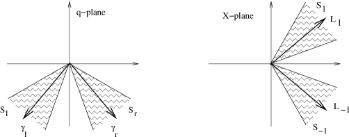
Figure 1: The $\gamma:=\gamma_{r}-\gamma_{l}$ and $L:=L_{1}-L_{-1}$ in $q$-plane and $X$-plane respectively.

Since $\phi_{n}(q)$ is an eigenfunction, $\phi_{n}(-iX)$ must vanish exponentially at infinity in both $S_{\pm 1}$. So, there exists a non-zero constant $\alpha_{n}$ such that

$$\phi_{n}(-iX)=\alpha_{n}Y_{1}(X,E_{n})=\alpha_{n}Y_{-1}(X,E_{n})$$

When $X$ take real values, we can deduce from (27) and (36) that $Y_{\pm 1}(X,E_{n})$ and $\phi_{n}(-iX)$ are all real. Hence, $\alpha_{n}\in\mathbb{R}$.

By Theorem 8, we have

$$\|\phi_{n}\|_{\mathcal{PT}}^{2}=i2\alpha_{n}^{2}C^{\prime}(E_{n})$$

The proof is complete by setting $K_{n}:=2\alpha_{n}^{2}$. ∎

The following result is a direct consequence of the theorem:

Corollary 9.1.

Assume that $E_{n}$ is a real eigenvalue of $H$, then $\|\phi_{n}\|_{\mathcal{PT}}^{2}=0$ if the multiplicity of $E_{n}$ is greater than $1$.

We now remind a classical result from real analysis:

Lemma 10.

Suppose that a real-valued function $f(x)$ is continuously differentiable on $(a,b)$ and $x_{1},x_{2}\in(a,b)$ are its two consecutive zeros. Then $f^{\prime}(x_{1})f^{\prime}(x_{2})\leq 0$.

Proof.

Assume conversely that $f^{\prime}(x_{1})f^{\prime}(x_{2})>0$; for instance $f^{\prime}(x_{1})>0$ and $f^{\prime}(x_{2})>0$. We deduce from this assumption that $f(x)$ increases strictly in sufficiently small neighborhoods of $x_{1}$ and $x_{2}$. This implies that $f(x_{1}+\epsilon)>0$ and $f(x_{2}-\epsilon)<0$ for a sufficiently small $\epsilon>0$. By its continuity, $f(x)$ must vanish at least once in the interval $(x_{1}+\epsilon,x_{2}-\epsilon)$. This is contrary to the hypothesis. ∎

This lemma asserts that if all zeros $x_{n}$ of $f(x)$ are simple then $f^{\prime}(x_{n})$ changes its sign alternatively. Hence a switch like $(-1)^{n}$. This is exactly what we describe in the next theorem.

Theorem 11.

Assume that all eigenvalues $E_{n}$ of the problem (28) are real and simple. Then, up to a normalization, the set of the corresponding eigenfunctions $\{\phi_{n}\},n\geq 0$, is $\mathcal{PT}$-orthonormal in the sense that

$$\ll\phi_{n},\phi_{m}\gg_{\mathcal{PT}}\;=\pm(-1)^{n}\delta_{mn}$$ (37)

where $\pm 1=\ll\phi_{0},\phi_{0}\gg_{\mathcal{PT}}$.

Proof.

We first notice that the reality of the whole set of eigenvalues $\{E_{n}\}$ enables us to treat $C(E):=C(a,E)$ as a function of the real variable $E$ (for each fixed $a\in\mathbb{R}^{m-1}$). This function is purely imaginary because of (25). Hence, $-iC(E)={\rm Im}C(E)$ is a real-valued function of $E\in\mathbb{R}$. So also is $-iC^{\prime}(E)$.

For $m\neq n$, the equality (37) is a direct consequence of Corollary 2.1. We should note that, as $m=n$, the sign of $\|\phi_{n}\|_{\mathcal{PT}}^{2}$ does not change when multiplying $\phi_{n}$ by a non-zero constant. Therefore, by applying lemma 10 to $-iC(E)$ and normalizing $\phi_{n}$, we get the conclusion. ∎

We emphasize that the hypothesis on the simpleness of all eigenvalues in this theorem is crucially necessary. Nevertheless, this requirement is not always satisfied, especially in cases of Hamiltonians involving parameters.

To end this section, we now detail the striking case when all $a_{j}=0$ and $m\geq 2$. The Hamiltonian then becomes $H=p^{2}+q^{2}(iq)^{m-2}$, whose whole eigenvalues have been proved to be real and positive using several different methods (see [6, 7, 15, 17, 19, 31]).

In their recent papers [2, 3], Bender et al showed that for some unbroken $\mathcal{PT}$-symmetric Hamiltonians, the charge operator $\mathcal{C}$ can be computed explicitly using perturbative techniques. They also provided numerical evidences on the sign alternation of $\|\phi_{n}\|_{\mathcal{PT}}^{2}$. We can now explain this phenomenon quite simply.

Let’s agree on the simpleness of all eigenvalues $E_{n}$, which will be the matter of a forthcoming paper, so that each $-iC^{\prime}(E_{n})$ possesses a sign. Note that by construction, the entire function $Y_{0}(X,E)$ is the solution (unique by its asymptotic behavior at infinity) of equation (29) which vanishes exponentially at $+\infty$ and takes only real-values whenever $X$ and $E$ are real. It is not hard to verify that $Y_{0}(0,0)\neq 0$. Therefore, substituting $X=0$ and $E=0$ in (27) yields

$$\omega^{-m/4}Y_{0}(0,0)=C(0)Y_{0}(0,0)+\omega^{m/4}Y_{0}(0,0)$$

This implies immediately that

$$-iC(0)=\frac{\omega^{-m/4}-\omega^{m/4}}{i}=2\sin\Big{(}\frac{2m\pi}{2(m+2)}\Big{)}>0$$

One can regard $-iC(E)$ now as a (real-valued) function of $E\in\mathbb{R}$ with only simple zeros $0<E_{0}<E_{1}<\cdots$ and starting with a positive value $-iC(0)>0$. As a direct consequence of lemma 10, we obtain

$${\rm sign}(-iC^{\prime}(E_{n}))=(-1)^{n+1}\ ;\quad\forall n\in\mathbb{N}$$

Then after normalizing $\phi_{n}$, we finally find out

$$\|\phi_{n}\|_{\mathcal{PT}}^{2}=(-1)^{n}\,,\qquad{\rm for}\quad n=0,1,2,3,\ldots$$

4. Conclusion

In this paper, we have established an explicit relation between $\mathcal{PT}$-pseudo-norm and the derivative of the Stokes multiplier $C(E)$ with respect to the eigenparameter. In this formulation, the indefiniteness of the $\mathcal{PT}$-pseudo-norm associated with a non-Hermitian but $\mathcal{PT}$-symmetric Hamiltonian is interpreted as a natural sign alternation of the derivative of an entire function at its zeros. This relation also supplies us a simple criterion to recognize degenerate eigenstates in the sense that their $\mathcal{PT}$-pseudo-norms are vanishing.

By Corollary 9.1, one has to acknowledge the unavoidable occurrence of such degenerate eigenstates, even if the corresponding eigenvalues are real. The reality of the whole spectral set of a $\mathcal{PT}$-symmetric Hamiltonian does not completely ensure the non-degeneracy of its eigenstates. This observation indicates that the unbroken $\mathcal{PT}$-symmetry is not exactly equivalent to the reality of the whole set of eigenvalues of a $\mathcal{PT}$-symmetric Hamiltonian.

To strengthen our arguments on this point, we should refer to an earlier joint work with Delabaere [17], where the spectrum of the Hamiltonian $H_{\alpha}=p^{2}+i(q^{3}+\alpha q)$ is investigated by means of (exact) semiclassical analysis. This Hamiltonian exhibits a version of a degeneracy of its eigenvalues $E_{n}=E_{n}(\alpha)$ for negative real $\alpha$. More precisely, when $\alpha$ goes to $-\infty$, some pairs of real eigenvalues gradually turn into complex conjugate. For the first critical value of $\alpha$ where this phenomenon occurs, the corresponding pairs of eigenvalues are nothing but double zeros of $C(E)$, which means that $C^{\prime}(E)=0$ at these zeros. Such a critical value has been computed in [21] $\alpha_{crit}\simeq-2.6118094$, and the eigenvalues becoming complex conjugate are the two lowest ones (see [17], Fig.1). We should notice that in this situation, the eigenvalues of $H_{\alpha_{crit}}$ are still all real.

Obviously, the action of the charge operator $\mathcal{C}$ (if any exists) on eigenfunctions in case of degeneracy may be not merely to switch signs by multiplying $\phi_{n}$ by $(-1)^{n}$ as in [3, 5]. Nevertheless, since there are at most a finite number of such degenerate eigenfunctions, we believe that an analogous method as those in the above citations could be still applicable to define the charge operator $\mathcal{C}$.

Findings on the indefiniteness of $\mathcal{PT}$-pseudo-norm enable us to keep on constructing the mathematical apparatus for $\mathcal{PT}$-symmetric quantum mechanics. In this study, the structure of a Krein space may be involved.

Moreover, there seems to exist some hidden relations between the Stokes multiplier $C(E)$ and the calculation of the charge operator $\mathcal{C}$. At least as we indicated, the simpleness and the reality of all the zeros of $C(E)$ first lead to the non-degeneracy of $\mathcal{PT}$-pseudo-norm, which is a necessary condition to construct this operator.

Acknowledgments.

This work was supported by the Abdus Salam International Centre for Theoretical Physics (ICTP) in the framework of Post-doctoral Fellowship.

References

- [1] B. Bagchi, C. Quesne, M. Znojil, Generalized Continuity Equation and Modified Normalization in PT-Symmetric Quantum Mechanics. Mod. Phys. Lett. A16 (2001) 2047-2057.
- [2] C.M. Bender, D.C. Brody; H.F. Jones, Must a Hamiltonian be Hermitian? Amer. J. Phys. 71 (2003), no. 11, 1095–1102.
- [3] C.M. Bender, J. Brod, A. Refig, M. E Reuter, The operator in -symmetric quantum theories J. Phys. A: Math. Gen. 37 No 43 (2004) 10139-10165.
- [4] C.M. Bender, M. Berry, A. Mandilara, Generalized symmetry and real spectra. J. Phys. A 35 (2002), no. 31, L467–L471.
- [5] C.M. Bender, P.N. Meisinger, Q.Wang, Calculation of the hidden symmetry operator in -symmetric quantum mechanics. J. Phys. A 36 (2003), no. 7, 1973–1983.
- [6] C.M. Bender, S. Boettcher, Real spectra in non-Hermitian hamiltonians having PT-symmetry. Phys. Rev. Lett. 80, 5243 (1998).
- [7] C.M. Bender, S. Boettcher, P.N. Meisinger, PT-symmetric quantum mechanics. J. Math. Phys. 40, 2201 (1999).
- [8] C.M. Bender, K.A. Milton, Model of supersymmetric quantum field theory with broken parity symmetry. Physical Review D, Vol 57, No 6, 3595-3608 (1998)
- [9] C.M. Bender, T.T. Wu, Anharmonic oscillator. Phys. Rev. 184, 1231-1260 (1969).
- [10] R. Ph. Jr. Boas, Entire functions. Academic Press Inc., New York, 1954.
- [11] E. Caliceti, S. Graffi, M. Maioli, Perturbation theory of odd anharmonic oscillators. Commun. Math. Phys. 75, 51-66 (1980).
- [12] F. Cannata, G. Junker, J. Trost, Schrödinger operators with complex potential but real spectrum. Phys. Lett. A 246, 219-226 (1998).
- [13] E. Delabaere, F. Pham, Unfolding the quartic oscillator. Annals of Physics 261, No. 2, 180-218 (1997).
- [14] E. Delabaere, H. Dillinger, F. Pham, Exact semi-classical expansions for one dimensional quantum oscillators. Journal Math. Phys. 38, 12, 6126-6184 (1997).
- [15] E. Delabaere, F. Pham, Eigenvalues of complex hamiltonians with -symmetry I. Phys. Lett. A 250, 25 (1998).
- [16] E. Delabaere, F. Pham, Eigenvalues of complex hamiltonians with -symmetry II. Phys. Lett. A 250, 29 (1998).
- [17] E. Delabaere, D.T. Trinh, Spectral analysis of the complex cubic oscillator. J.Phys. A: Math. Gen. 33 (2000), 8771-8796.
- [18] E. Delabaere, J.-M. Rasoamanana, Resurgent deformations for an ordinary differential equation of order 2. To appear in Pacific Journal of Mathematics.
- [19] P. Dorey, C. Dunning, R. Tateo, Spectral equivalences, Bethe ansatz equations, and reality properties in -symmetric quantum mechanics. J. Phys. A 34 (2001), no. 28, 5679–5704.
- [20] F.M. Fernández, R. Guardiola, J. Ros, M. Znojil, A family of complex potentials with real spectrum. J. Phys. A 32, No. 17, 3105-3116 (1999).
- [21] C.R. Handy, Generating converging bounds to the (complex) discrete states of the Hamiltonian. J. Phys. A 34 (2001), no. 24, 5065–5081
- [22] G.S. Japaridze, Space of state vectors in symmetrical quantum mechanics J. Phys. A 35 (2002), no. 7, 1709–1718.
- [23] G. Lévai, M. Znojil, Conditions for complex spectra in a class of -symmetric potentials. Modern Phys. Lett. A 16 (2001), no. 30, 1973–1981.
- [24] G. Lévai, F.Cannata, A.Ventura, -symmetry breaking and explicit expressions for the pseudo-norm in the Scarf II potential. Phys.Lett.A 300 (2002) 271–281.
- [25] G.A Mezincescu, Some properties of eigenvalues and eigenfunctions of the cubic oscillator with imaginary coupling constant. J. Phys. A. 33 (2000).
- [26] A. Mostafazadeh, Pseudo-Hermiticity versus symmetry: the necessary condition for the reality of the spectrum of a non-Hermitian Hamiltonian. J. Math. Phys. 43 (2002), no. 1, 205–214.
- [27] A. Mostafazadeh, Exact -symmetry is equivalent to Hermiticity . J. Phys. A: Math. Gen. 36 No 25 (2003) 7081-7091.
- [28] A. Mostafazadeh, A.Batal, Physical aspects of pseudo-Hermitian and -symmetric quantum mechanics . J. Phys. A: Math. Gen. 37 No 48 (2004) 11645-11679.
- [29] F. Pham, Confluence of turning points in exact WKB analysis. The Stokes phenomenon and Hilbert’s 16th problem (Groningen, 1995), 215–235, World Sci. Publishing, River Edge, NJ (1996).
- [30] F. Pham, Multiple turning points in exact WKB analysis (variations on a theme of Stokes). Toward the exact WKB analysis of differential equations linear or non-linear (C.Howls, T.Kawai, Y.Takei ed.), Kyoto University Press (2000),71-85.
- [31] K.C. Shin, On the reality of the eigenvalues for a class of -symmetric oscillators. Comm. Math. Phys. 229 (2002), no. 3, 543–564.
- [32] Y. Sibuya, Global Theory of a Second Order Linear Differential Equation with a Polynomial Coefficient. Mathematics Studies 18, North-Holland Publishing Company (1975).
- [33] T.D. Tai, Asymptotique et analyse spectrale de l’oscillateur cubique. Thèse, Université de Nice (2002).
- [34] T.D. Tai, On the Sturm-Liouville problem for the complex cubic oscillator. Asymptotic Analysis, 40 (2004), no. 3-4, 211-234.
- [35] A. Voros, The return of the quartic oscillator. The complex WKB method Ann. Inst. H.Poincaré, Physique Théorique, 39, 211-338 (1983).
- [36] A. Voros, Exact resolution method for general polynomial Schrödinger equation. J. Phys. A 32, No. 32, 5993–6007 (1999).
- [37] M. Znojil, Conservation of pseudo-norm in PT symmetric quantum mechanics. Rend. Circ. Mat. Palermo (2) Suppl. No. 72 (2004), 211–218.
- [38] M. Znojil, -symmetrized supersymmetric quantum mechanics. DI-CRM Workshop on Mathematical Physics (Prague, 2000). Czechoslovak J. Phys. 51 (2001), no. 4, 420–428.
- [39]