MHD $\alpha^{2}-$dynamo, Squire equation and ${\cal PT}-$symmetric interpolation between square well and harmonic oscillator

Abstract

It is shown that the $\alpha^{2}-$dynamo of Magnetohydrodynamics, the hydrodynamic Squire equation as well as an interpolation model of ${\cal PT}-$symmetric Quantum Mechanics are closely related as spectral problems in Krein spaces. For the $\alpha^{2}-$dynamo and the ${\cal PT}-$symmetric model the strong similarities are demonstrated with the help of a $2\times 2$ operator matrix representation, whereas the Squire equation is re-interpreted as a rescaled and Wick-rotated ${\cal PT}-$symmetric problem. Based on recent results on the Squire equation the spectrum of the ${\cal PT}-$symmetric interpolation model is analyzed in detail and the Herbst limit is described as spectral singularity.

1 Introduction

Non-Hermitian ${\cal PT}-$symmetric quantum mechanical systems [1, 2, 3, 4, 5, 6, 7, 8] are known to possess spectral sectors with purely real eigenvalues as well as sectors with pairs of complex conjugate eigenvalues. Changes of certain system parameters can lead to spectral phase transitions from one sector to the other. The physics in the two sectors has been identified with phases of unbroken ${\cal PT}-$symmetry (real eigenvalues) and spontaneously broken ${\cal PT}-$symmetry (pairwise complex conjugate eigenvalues) [1, 2]. From a mathematical point of view, non-Hermitian ${\cal PT}-$symmetric Hamiltonians are self-adjoint operators in Krein spaces [9, 10, 11] — Hilbert spaces with an additional indefinite metric structure — and the two spectral sectors correspond to Krein space states of positive or negative type (real eigenvalues) and neutral (isotropic) states (pairwise complex conjugate eigenvalues).

Apart from ${\cal PT}-$symmetric Quantum Mechanics (PTSQM), it is known that a certain class of spherically symmetric mean-field dynamo models [12] of Magnetohydrodynamics (MHD) can be described by self-adjoint operators in Krein spaces as well [13]. These models show similar spectral phase transitions from real to pairwise complex conjugate eigenvalues [14] — and only the physical interpretation differs from that in PTSQM. For dynamos it simply consists in a transition from non-oscillatory states to oscillatory states.

In the present paper, we are going to briefly describe the underlying structural operator theoretic parallels between PTSQM models and the spherically symmetric MHD $\alpha^{2}-$dynamo (section 2). The discussion will be illustrated with the help of a ${\cal PT}-$symmetric interpolation between a harmonic oscillator placed in a square well and an empty square well (section 3). This interpolation shows a rich structure of spectral phase transitions with a couple of unexpected features. Furthermore, we will show in sect. 4 that the eigenvalue problem of the ${\cal PT}-$symmetric (intermediate) interpolation model with linear complex potential (purely complex electrical field) within the square well is mathematically identical to the eigenvalue problem of the rescaled and Wick-rotated Squire equation of hydrodynamics which describes the normal vorticity of a plane channel flow (Couette flow) with linear transversal velocity profile. Recent Airy function based results on the Squire equation allow us to analytically describe the spectral behavior of the PTSQM model in the limiting case when the width of the square well tends to infinity. In this limit we reproduce the Herbst model [15] with its empty spectrum. The limiting behavior occurs as a blowing-up of the spectrum to infinity along three directions on the complex plane — leaving behind a spectrally empty region at any fixed finite distance from the origin of the spectral plane. In section 5 we briefly sketch some links of the obtained results to other physical setups and analytical techniques.

2 Krein space properties of ${\cal PT}-$symmetric quantum models and of the spherically symmetric MHD $\alpha^{2}-$dynamo

2.1 ${\cal PT}-$symmetric quantum models

In their seminal letter [1] Bender and Boettcher identified ${\cal PT}-$symmetry as the essential property of the non-Hermitian quantum system

$$H\psi(x)=E\,\psi(x),\ \ \ \ \ \ \ \ \ \ \ \ \ \ H=-\frac{d^{2}}{dx^{2}}+g\,x^{2}(ix)^{\nu}$$ (1)

which ensures the reality of its spectrum for exponents $\nu\in[0,2)$ and $\psi(x)\in\tilde{\cal H}=L_{2}(-\infty,\infty)$ [16]. This allowed them not only to extend an earlier conjecture of Bessis and Zinn-Justin (whose numerical results indicated that quantum systems with complex potential $V(x)=ix^{3}$ might have a purely real spectrum), but also initiated the still lasting intensive study of generalized ${\cal PT}-$symmetric non-Hermitian systems [17]. Such systems are characterized by a ${\cal PT}-$symmetric Hamiltonian $H$,

$$[{\cal PT},H]=0$$ (2)

where ${\cal P}$ denotes a reflection

$${\cal P}x{\cal P}=-x,\qquad{\cal P}\psi(x)=\psi(-x)$$ (3)

while the time-reversal operator ${\cal T}$ performs complex conjugation

$${\cal T}i{\cal T}=-i,\qquad{\cal T}\psi(x)=\psi(x)^{*}.$$ (4)

Because both operators ${\cal P}$ and ${\cal T}$ are involution operators,

$${\cal P}^{2}=I,\qquad{\cal T}^{2}=I,$$ (5)

they induce natural ${\mathbb{Z}}_{2}-$gradings of the Hilbert space $\tilde{\cal H}$. For our subsequent analysis it suffices to consider the subclass of models which can be defined solely over the real line $x\in{\mathbb{R}}$. For such models the ${\cal T}-$induced ${\mathbb{Z}}_{2}-$grading corresponds to a splitting of the wave functions $\psi\in\tilde{\cal H}$ into real and imaginary components (what is of no direct physical interest in a quantum mechanical context; additionally one would have to work in a real Hilbert space with doubled dimension compared to the original complex one), whereas ${\cal P}$ induces a ${\mathbb{Z}}_{2}-$grading into parity even and parity odd components

$$\psi(x)=\psi_{+}(x)+\psi_{-}(x),\qquad{\cal P}\psi_{\pm}(x)=\psi_{\pm}(-x)=\pm\psi_{\pm}(x)\,.$$ (6)

The corresponding ${\mathbb{Z}}_{2}-$graded Hilbert space splits as

$$\tilde{\cal H}={\cal H}_{+}\oplus{\cal H}_{-},\qquad\psi_{\pm}\in{\cal H}_{\pm}\,.$$ (7)

In the case of a simple ${\cal PT}-$symmetric one-particle system with Hamiltonian

$$H=-\partial^{2}_{x}+V_{+}(x)+iV_{-}(x),\qquad V_{\pm}(-x)=\pm V_{\pm}(x),\quad\Im V_{\pm}=0$$ (8)

it holds

$$H={\cal P}H^{\dagger}{\cal P}$$ (9)

and ${\cal P}$ is a so called fundamental (canonical) operator symmetry [9, 10] of $H$ — i.e., $H$ is ${\cal P}-$pseudo-Hermitian in the sense of Refs. [4, 5]. Operators with an involutive fundamental symmetry are known to be symmetric — and for appropriately chosen domain (boundary conditions for the functions $\psi(x)$) even self-adjoint — in a Krein space $\cal{K}$. For ${\cal P}-$pseudo-Hermitian operators over the real line this Krein space $\cal{K}_{\cal P}$ is given as [11, 18, 19]

$$\left(\cal{K}_{\cal P},[.,.]_{\cal P}\right),\qquad[\psi,\phi]_{\cal P}=(\psi,{\cal P}\phi)=\int_{C\subseteq{\mathbb{R}}}\psi^{*}(x){\cal P}\phi(x)dx=\int_{C\subseteq{\mathbb{R}}}\psi^{*}(x)\phi(-x)dx\,.$$ (10)

Depending on the concrete problem, the integration in (10) is performed over a finite interval, $C=[-a,a]$, or over the complete real line, $C=(-\infty,\infty)\sim{\mathbb{R}}$. From (8), (9) one immediately finds

$$[H\psi,\phi]_{\cal P}=[\psi,H\phi]_{\cal P}\,.$$ (11)

The Krein space inner (scalar) product $[\psi,\phi]_{\cal P}$ has the following properties:

• It coincides with the more general ${\cal PT}$ inner product of C. Bender et al [6, 7]

  $$(\psi,\phi)_{\cal PT}=\int_{C\subset{\mathbb{C}}}[{\cal PT}\psi(x)]\phi(x)dx$$ (12)

  when the integration path $C\subset{\mathbb{C}}$ of the latter integral is restricted to (an interval of) the real line, $C\subseteq{\mathbb{R}}$,

  $$(\psi,\phi)_{\cal PT}=\int_{C\subseteq{\mathbb{R}}}[{\cal PT}\psi(x)]\phi(x)dx=\int_{C\subseteq{\mathbb{R}}}[{\cal P}\psi(x)^{*}]\phi(x)dx=\int_{C\subseteq{\mathbb{R}}}\psi(x)^{*}{\cal P}\phi(x)=[\psi,\phi]_{\cal P}\,.$$ (13)

• In contrast to the ”usual” positive definite metric structure of the Hilbert space $\tilde{\cal H}={\cal H}_{+}\oplus{\cal H}_{-}$,

  $$\left(\tilde{\cal H},(.,.)\right),\qquad(\psi,\phi)=\int_{C\subseteq{\mathbb{R}}}\psi^{*}(x)\phi(x)dx=\int_{C\subseteq{\mathbb{R}}}\left(\psi^{*}_{+}\phi_{+}+\psi^{*}_{-}\phi_{-}\right)dx\,,$$ (14)

  with non-negative norm

  $$||\psi||^{2}=(\psi,\psi)=||\psi_{+}||^{2}+||\psi_{-}||^{2}\geq 0\,,$$ (15)

  the scalar product $[\psi,\phi]_{\cal P}$ defines an indefinite metric structure in the Krein space $\cal{K}_{\cal P}={\cal H}_{+}\oplus{\cal H}_{-}$, what is easily seen from the decomposition (6)

  $$[\psi,\phi]_{\cal P}=\int_{C\subseteq{\mathbb{R}}}\left(\psi_{+}^{*}\phi_{+}-\psi_{-}^{*}\phi_{-}\right)dx.$$ (16)

• In rough analogy with time-like, space-like, and light-like (isotropic) vectors in Minkowski space, one distinguishes Krein space vectors of positive type, $[\psi_{+},\psi_{+}]_{\cal P}=||\psi_{+}||^{2}>0$, of negative type, $[\psi_{-},\psi_{-}]_{\cal P}=-||\psi_{-}||^{2}<0$, and neutral (isotropic) vectors:

  $$[\psi,\psi]_{\cal P}=0,\quad\psi=\psi_{+}+\psi_{-},\quad||\psi_{+}||^{2}=||\psi_{-}||^{2}\,.$$ (17)

In order to make the structural Krein space analogies of PTSQM models and MHD dynamo setups maximally transparent, we rewrite the eigenvalue problem, $H\psi=E\psi$, for the ${\cal PT}-$symmetric Hamiltonian (8) in an equivalent $2\times 2$ matrix operator representation. Introducing the projection operators

$$P_{\pm}:=\frac{1}{2}(I\pm{\cal P})$$ (18)

we decompose wave function $\psi$ and Hamiltonian $H$ (see, e.g., [9]) as

$$\psi = P_{+}\psi+P_{-}\psi=\psi_{+}+\psi_{-}$$ (19)

$$H = P_{+}HP_{+}+P_{-}HP_{+}+P_{+}HP_{-}+P_{-}HP_{-}\,.$$ (20)

In terms of the notation

$$H_{\pm\pm}:=P_{\pm}HP_{\pm}=-\partial^{2}_{x}+V_{+}(x),\qquad H_{\pm\mp}:=P_{\pm}HP_{\mp}=iV_{-}(x)$$ (21)

this gives

$$\left(\begin{array}[]{cc}H_{++}&H_{+-}\\ H_{-+}&H_{--}\end{array}\right)\left(\begin{array}[]{c}\psi_{+}\\ \psi_{-}\end{array}\right)=E\left(\begin{array}[]{c}\psi_{+}\\ \psi_{-}\end{array}\right),\qquad{\cal P}=\left(\begin{array}[]{cc}I&0\\ 0&-I\end{array}\right)\,,$$ (22)

where

$$H_{\pm\pm}=H_{\pm\pm}^{\dagger},\qquad H_{+-}=-H_{-+}^{\dagger}\,.$$ (23)

If one replaces the matrix entries in (22), (23) by appropriate constants one arrives at the schematic two-level model

$$H_{H}\left(\begin{array}[]{c}u\\ v\end{array}\right)=E\,\left(\begin{array}[]{c}u\\ v\end{array}\right),\qquad H_{H}=\left(\begin{array}[]{cc}c+a&b\\ -b^{*}&c-a\end{array}\right),\quad a,c\in{\mathbb{R}}\,,$$ (24)

which may be read as an elementary exemplification of Heisenberg’s linear-algebraic approach [20] to (${\cal PT}-$symmetric) Quantum Mechanics and which was intensively studied in Refs. [6, 7, 18, 21, 22, 23].

2.2 The spherically symmetric MHD $\alpha^{2}-$dynamo

The magnetic fields of planets, stars and galaxies are maintained by homogeneous dynamo effects, which can be successfully described within magnetohydrodynamics (MHD). One of the simplest dynamos is the spherically symmetric mean-field $\alpha^{2}-$dynamo in its kinematic regime. This dynamo model is capable to play a similar paradigmatic role in MHD dynamo theory like the harmonic oscillator in Quantum Mechanics (QM). Its operator matrix has the form [13]

$$\hat{H}_{l}[\alpha]=\left(\begin{array}[]{cc}-Q[1]&\alpha\\ Q[\alpha]&-Q[1]\end{array}\right)$$ (25)

and consists of formally selfadjoint blocks

$$Q[\alpha]:=p\alpha p+\alpha\frac{l(l+1)}{r^{2}}\,,$$ (26)

where $p=-i(\partial_{r}+1/r)$ denotes the radial momentum operator. The operator $\hat{H}_{l}[\alpha]$ is defined over an interval $\Omega=[0,1]\ni r$ and acts on two-component vectors $\phi$ which describe the coupled $l-$modes of the poloidal and toroidal magnetic field components of a mean-field dynamo model with helical turbulence function ($\alpha-$profile) $\alpha(r)$.

Although the dynamo model is not ${\cal PT}-$symmetric, its operator $\hat{H}_{l}[\alpha]$ shares a basic underlying symmetry with PTSQM Hamiltonians — a ${\mathbb{Z}}_{2}-$graded pseudo-Hermiticity ($J-$pseudo-Hermiticity) [5, 14] which is induced by the fundamental (canonical) symmetry:

$$\hat{H}_{l}[\alpha]=J\hat{H}_{l}^{\dagger}[\alpha]J,\qquad J=\left(\begin{array}[]{cc}0&I\\ I&0\end{array}\right)\,.$$ (27)

Similar to the reflection operator ${\cal P}$ in (9), the operator $J$ is unitary and involutive

$$J^{\dagger}=J^{-1},\qquad J^{2}=I.$$ (28)

The boundary conditions on the vector function $\phi$ are set at $r=1$ (the rescaled surface radius of the star or planet whose fluid/plasma motion maintains the dynamo effect) and it is assumed that $\alpha(r>1)\equiv 0$. In the case of physically idealized boundary conditions at $r=1$ (see, e.g., Ref. [24]), the domain ${\cal D}(\hat{H}_{l}[\alpha])$ of the operator $\hat{H}_{l}[\alpha]$ consists of functions $\phi$ such that

$${\cal D}(\hat{H}_{l}[\alpha]) :=\left\{\phi=\left(\begin{array}[]{r}\phi_{1}\\ \phi_{2}\end{array}\right):\ \phi\in\tilde{{\cal H}}\equiv{\cal H}\oplus{\cal H},\ {\cal H}=L_{2}(\Omega,r^{2}dr),\right.$$ (31)

$$\left.\Omega=[0,1],\ \phi(1)=0,\ \left.r\phi(r)\right|_{r\to 0}\to 0\right\},$$ (32)

and $\hat{H}_{l}[\alpha]$ is self-adjoint in a Krein space

$$\left(\cal{K}_{J},[.,.]_{J}\right),\qquad[\psi,\phi]_{J}=\int_{0}^{1}\psi^{\dagger}J\phi\,\,r^{2}dr,$$ (33)

$$[\hat{H}_{l}\chi,\phi]_{J}=[\chi,\hat{H}_{l}\phi]_{J}\,.$$ (34)

It should be noted that for physically realistic boundary conditions

$$\left.\hat{B}_{l}\phi\right|_{r=1}=0,\qquad\hat{B}_{l}=\mbox{diag}[\partial_{r}+(l+1)/r,1]$$ (35)

there exists no appropriate Krein space which could make the operator $\hat{H}_{l}[\alpha]$ $J-$self-adjoint.

The structures of PTSQM models and the $\alpha^{2}-$dynamo can be compared most explicitly after passing from $\cal{K}_{J}$ to an equivalent Krein space $\cal{K}_{\mu}$ with diagonal metric operator $\mu$ and redefined Hilbert spaces components, $L_{2}(\Omega,r^{2}dr)\mapsto L_{2}(\Omega,dr)$. The diagonalization yields

$$J\mapsto\mu:=\left(\begin{array}[]{rr}I&0\\ 0&-I\end{array}\right)=S^{-1}JS,\quad S=\frac{1}{\sqrt{2}}\left(\begin{array}[]{rr}I&-I\\ I&I\end{array}\right)\,,$$ (36)

$$\hat{H}_{l}[\alpha]\mapsto\check{H}_{l}[\alpha]=S^{-1}\hat{H}_{l}[\alpha]S=\frac{1}{2}\left(\begin{array}[]{ccc}Q[\alpha-2]+\alpha&&-Q[\alpha]+\alpha\\ Q[\alpha]-\alpha&&Q[-\alpha-2]-\alpha\end{array}\right),$$ (37)

$$\phi\mapsto\check{\phi}=\left(\begin{array}[]{c}\phi_{+}\\ \phi_{-}\end{array}\right)=\frac{1}{\sqrt{2}}\left(\begin{array}[]{c}\phi_{2}+\phi_{1}\\ \phi_{2}-\phi_{1}\end{array}\right),$$ (38)

whereas the unitary mapping $U:\ L_{2}(\Omega,r^{2}dr)\mapsto L_{2}(\Omega,dr)$ simplifies the structure of $Q[\alpha]$ and leads in (37), (38) to the additional replacements

$$\phi_{1,2}\mapsto f_{1,2}:=r\phi_{1,2},\qquad Q[\alpha]\mapsto q[\alpha]:=rQ[\alpha]r^{-1}=-\partial_{r}\alpha(r)\partial_{r}+\alpha(r)\frac{l(l+1)}{r^{2}}\,.$$ (39)

By inspection of (21) - (23) and (36) - (39) we find that, in the chosen Krein space representations of the PTSQM model and the $\alpha^{2}-$dynamo, the block structures of the metrics (involution operators) ${\cal P}$ and $\mu$ coincide, ${\cal P}=\mu$, but that the blocks of the ${\cal PT}-$symmetric Hamiltonian and the dynamo operator show significant structural differences:

$$H_{\pm\pm}=-\partial_{x}^{2}+V_{+}(x) \qquad\longleftrightarrow\qquad -q[1]\pm\frac{q[\alpha]+\alpha}{2}\,,$$

$$H_{\pm\mp}=iV_{-}(x) \quad\longleftrightarrow\quad \mp\frac{q[\alpha]-\alpha}{2}\,.$$ (40)

It is clear that these differences in the differential expressions (as well as the different boundary conditions on the two-component eigenfunctions) will lead to different global behaviors of the corresponding operator spectra. Nevertheless, both types of systems share the same Krein-space induced features of level crossings, what will be briefly sketched in the next subsection.

2.3 Spectral phase transitions

Since the first PTSQM paper [1] of Bender and Boettcher it is known that ${\cal PT}-$symmetric Hamiltonians have a real spectrum when ${\cal PT}-$symmetry is an exact symmetry and not spontaneously broken (the corresponding eigenfunctions are invariant under a ${\cal PT}-$transformation), whereas spontaneously broken ${\cal PT}-$symmetry is connected with complex energies. A consistent PTSQM applicability and interpretation of the complex-energy states remains an open question up to now (cf., e.g., [26]). For convenience, we shall call these states ”unphysical” here.

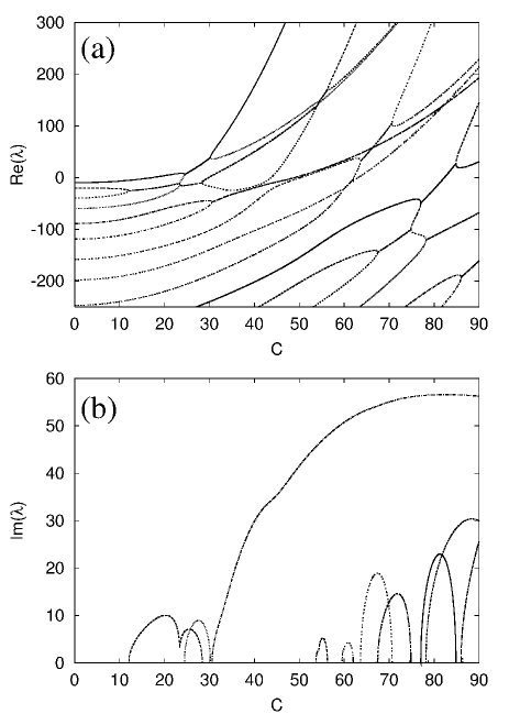
Figure 1: Real and imaginary components of the $\alpha^{2}-$dynamo spectrum as functions of the scale factor $C$ of an $\alpha-$profile $\alpha(r)=C\times(1-26.09\times r^{2}+53.64\times r^{3}-28.22\times r^{4})$ in the case of angular mode number $l=1$ and physically realistic boundary conditions (35). The concrete coefficients in the quartic polynomial $\alpha(r)$ have their origin in numerical simulations of the field reversal dynamics (see Ref. [30]). Only the imaginary components with $\Im\lambda\geq 0$ are shown. The complex conjugate $(\Im\lambda\leq 0)-$components are omitted for sake of brevity.

The mathematically most interesting questions of PTSQM concern the transition between the physical and unphysical domains of their parameters. In the simple two-state model (24) it is easy to deduce that the quantized energies $E$ are real (“physical”) for $|a|>|b|$ while they form complex-conjugate pairs in the “unphysical” regime where $|a|<|b|$ [7, 18]. The boundary of its PTSQM applicability coincides with the double-cone hypersurface in parameter space where $|a|=|b|$. One easily verifies that whenever $|b|$ approaches $|a|$, the separate eigen-energies $E_{\pm}$ as well as the corresponding two independent bound-state eigenvectors coalesce and coincide. On the critical hypersurface the remaining (geometrical) eigen-vector becomes supplemented by a so called associated vector (algebraic eigen-vector) [14] and the Hamiltonian matrix $H$ acquires a Jordan-block canonical structure [14, 27]. The latter cannot be diagonalized and it only gives the doubly degenerate and real single “exceptional-point” eigenvalue $E=E_{(EP)}=c$ (cf., e.g., Ref. [28] for more details).

An exhaustive and consistent bound-state interpretation of the Schrödinger type equation (1) is more difficult. For example, it requires the restriction of the range of exponents to a finite interval of $\nu\in(-1,2)$ for $\psi(x)\in L_{2}(-\infty,\infty)$ as usual defined on the real line [1]. A rigorous proof of the reality of the energies turned out unexpectedly difficult [16, 29]. For larger exponents $\nu$, the real line must be replaced by an appropriately deformed contour in the complex plane [1, 2].

A systematic analytical study of phase transition points is still lacking for PTSQM models; the same concerns efficient mathematical tools for deriving their location in parameter space. Similar to the double-cone hyper-surfaces for the simple matrix model (24), one expects more complicated (and more interesting) global phase-transition hyper-surfaces in case of the Schrödinger type systems. Knowing the location of these phase transition hyper-surfaces, one would know the boundaries of the ”physical” regions of exact ${\cal PT}-$symmetry.

For the $\alpha^{2}-$dynamo both types of eigenvalues — real ones as well as pair-wise complex conjugate ones — have a clear physical meaning. They simply correspond to non-oscillatory and oscillatory dynamo states, respectively. But again it is of utmost interest to know the parameter configurations for which transitions between the two types of states (phases) occur. In the recent paper [30], strong numerical indications were presented that magnetic field reversals (interchanges of North and South poles as they are evident from paleo-magnetic data on the Earth magnetic field [31]) are induced by a special type of nonlinear dynamics in the vicinity of spectral phase transition points.

The qualitative features of the real-to-complex phase transitions are essentially the same for PTSQM models and for the MHD $\alpha^{2}-$dynamo. They correspond to transitions from Krein space states of positive and negative type to pair-wise neutral (isotropic) states [11, 14] — and a square-root branching of the spectral Riemann surface [33, 34]. Such transitions are a generic feature of Krein-space setups and they are new compared with setups in Hilbert spaces with purely positive metric structures as in ”usual” QM. The square-root branching behavior is easily seen by passing from the linear eigenvalue problems for the $2\times 2-$operator matrices $H$ and $\hat{H}_{l}[\alpha]$ of Eqs. (22) and (25),

$$(H-E)\psi=0,\qquad\left(\hat{H}_{l}[\alpha]-\lambda\right)\phi=0,$$ (41)

via substitutions

$$\psi=\left(\begin{array}[]{c}\psi_{+}\\ -\frac{1}{H_{+-}}\left[H_{++}-E\right]\psi_{+}\end{array}\right),\qquad\phi=\left(\begin{array}[]{c}\phi_{1}\\ \frac{1}{\alpha}\left[Q(1)+\lambda\right]\phi_{1}\end{array}\right)$$ (46)

to the equivalent quadratic operator pencils

$$\left\{(H_{--}-E)\frac{1}{H_{+-}}(H_{++}-E)-H_{-+}\right\}\psi_{+} = 0,$$

$$\left\{\left(Q[1]+\lambda\right)\frac{1}{\alpha}\left(Q[1]+\lambda\right)-Q[\alpha]\right\}\phi_{1} = 0.$$ (47)

Both pencils are of the same generic operator type

$$L[\lambda]\psi=\left[A_{2}\lambda^{2}+A_{1}\lambda+A_{0}\right]\psi=0$$ (48)

with a scalar product

$$(\psi,L[\lambda]\psi)=a_{2}\lambda^{2}+a_{1}\lambda+a_{0}=0,\quad a_{j}:=(\psi,A_{j}\psi)$$ (49)

which can be used to deduce the local square-root branching behavior of the spectrum

$$\lambda_{1,2}=\frac{1}{2a_{2}}\left(-a_{1}\pm\sqrt{a_{1}^{2}-4a_{0}a_{2}}\right).$$ (50)

A typical $\alpha^{2}-$dynamo spectrum with a large number of real-to-complex transitions is presented in Fig. 1 (see also Refs. [14, 35]). These crossings with real-to-complex transition occur at exceptional points (in the sense of Kato [36]) of (square root) branching type [37, 38] and the corresponding eigenvalues have geometric multiplicity one and algebraic multiplicity two [14]. In contrast, crossings without real-to-complex transitions are of the same type as level crossings in Hermitian systems [11] — with geometric and algebraic multiplicity two [39]. Finally, we note that although locally crossings with real-to-complex transitions occur, in general, only between two spectral branches, globally much more branches are involved in mutual crossings (see Fig. 1). This reflects the fact that in general the spectrum forms a multi-sheet Riemann surface over the parameter space of the theory (see e.g. [33, 34, 40]).

In the next section, we will analyze the spectral behavior of a ${\cal PT}-$symmetric interpolation model where we will find a similar rich structure of real-to-complex transitions as for the $\alpha^{2}-$dynamo.

3 ${\cal PT}-$symmetric interpolation between square well and harmonic oscillator

In Schrödinger-type models (1) over the open real line $x\in(-\infty,\infty)$ a PTSQM-related separation of the “physical” and “unphysical” domains is, in general, a mathematically highly non-trivial problem. Its resolution requires a fairly subtle and rigorous mathematical argumentation [16, 29]. A typical result of the WKB analysis of Ref. [1] was that in a half-open interval of $\nu\in[0,2)$ the energies remain real and that the ${\cal PT}-$symmetry of the wave functions remains unbroken. In parallel, a characteristic unphysical behavior of the system (1) has been found in the half-open interval of $\nu\in[-1,0)$, where at any $\nu<0$ all the sufficiently high-lying energies $E_{n}$ with $n>n_{0}(\nu)$ “decay” in complex-conjugate pairs, $\Im E_{n}\neq 0$. Moreover, the spectrum becomes empty in the Herbst-Hamiltonian limit of the leftmost $\nu=-1$ [1].

3.1 Toy model ${\cal PT}-$symmetric differential equation

In the present section, we are going to extend the consideration of the Schrödinger-type system (1) to exponents from the interval $\nu\in[-2,0]$. The end-points of this interval correspond to the purely real-valued Hermitian-system spectra of a freely moving particle with shifted off-set energy (for $\nu=-2$) and a harmonic oscillator (for $\nu=0$). For the exponents $\nu\in(-2,0)$ we expect a phase of spontaneously broken ${\cal PT}-$symmetry with an involved picture of real-to-complex spectral phase transitions.

In order to keep the numerical analysis sufficiently simple and robust, we assume the system located in a square well (box) of finite width $2b<\infty$ and Dirichlet boundary conditions imposed at the walls, $\psi(x=\pm b)=0$, i.e. we introduce an IR cut-off at the low-energy end of the spectrum. This enables us to rescale Eq. (1) to the equivalent equation

$$\left[-\partial_{y}^{2}+G\,y^{2}(iy)^{\nu}\right]\psi[x(y)]=\mu(E)\,\psi[x(y)]$$ (51)

with parameter-independent boundary conditions

$$\psi[x(\pm 1)]=0\,,$$ (52)

but rescaled coupling constant and energy

$$G=g\,b^{4+\nu},\ \ \ \ \ \ \ \ \ \ \ \ \mu(E)=b^{2}\,E\,.$$ (53)

In this notation, the original bound-state problem (1) with asymptotic Dirichlet boundary conditions at $x\to\pm\infty$ is replaced by the equivalent new problem defined within a fixed finite interval $[-1,1]$. In the limit of very small $b\approx 0$ the potential term becomes negligible, $G\approx 0$, and the interaction degenerates to an infinitely deep square well (box) at all $\nu$. A completely similar situation occurs for systems with any non-vanishing finite $b$, but very small exponents, $\nu\approx-2$. In both extremal cases the problem remains exactly solvable. The original Bender-Boettcher problem corresponds to the strong-coupling limit, $G\to\infty$, $b\to\infty$, with $g$ hold fixed, $g=G\,b^{-4-\nu}=\mbox{\rm const}$.

For finite coupling constants $0<G<\infty$ one expects the energy spectrum to be divided into three sectors: into a low-energy sector with states which are involved in real-to-complex phase transitions, into an intermediate sector, where the $\nu-$dependent energies still remain real, and into a high-energy sector with almost $\nu-$independent purely real eigenvalues whose states experience only a small perturbations from the complex interaction term. The division into low energy and intermediate-and-high energy sectors has been qualitatively described in a recent paper [11] by Langer and Tretter who considered a square well model with an arbitrary ${\cal PT}-$symmetric potential $V$ as perturbation. Starting from the energy spectrum of the empty square well, $\mu_{k}=k^{2}\pi^{2}/4$,  $k=1,2,\ldots\$, they showed that there are no real-to-complex phase transitions for levels $k>k_{s}$ with $k_{s}$ as the lowest level satisfying the supremum bound $||V||_{\infty}<(2k_{s}+1)\pi^{2}/8$. In case of our model with potential $V(y)=gb^{4+\delta}\,y^{2}(iy)^{\nu}$ the supremum norm (see, e.g., [43]) reads (for $\nu\geq-2$)

$$||V||_{\infty}=\sup_{y\in[-1,1]}|V(y)|=|V(\pm 1)|=|g|b^{4+\nu}$$ (54)

so that it is ensured that there are no phase transitions for levels

$$k>k_{s}(b)>\frac{1}{2}\left[\frac{8}{\pi^{2}}|g|b^{4+\nu}-1\right].$$ (55)

According to [11] it holds for the corresponding real eigenvalues $\mu_{k}$: $|\mu_{k}-k^{2}\pi^{2}/4|<|g|b^{4+\nu}$. The supremum bound is safe, but at the same time rather rough [44]. The subsequent exact numerical analysis shows that, depending on the concrete exponents $\nu$, the real-to-complex phase transitions in the model (51) stop at much lower energy levels.

3.2 The emergence of $\Im E\neq 0$ on certain finite subintervals of $\nu\in(-2,0)$

In the generic case with $\nu\in(-2,0)$ and $b>0$, we have solved Eqs. (51) + (52) numerically by means of a shooting technique with a fifth-order Runge-Kutta method, utilizing and adapting standard routines from Numerical Recipes [45]. The corresponding code had been validated extensively in earlier work by comparison with known analytical results and other numerical results in dynamo theory and quantum mechanics.

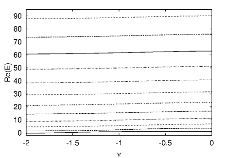
Figure 2: Spectrum of the ${\cal PT}-$symmetric interpolation Hamiltonian $H=-\partial^{2}_{x}+x^{2}\left(ix\right)^{\nu}$ as function of the exponent $\nu$ for the cut-off length $b=2$. All eigenvalues are real and almost independent of $\nu$. The spectrum is only slightly deviating from that of an empty square well.

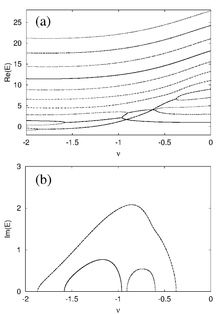
Figure 3: Real and imaginary components of the spectrum in the case of a cut-off length $b=4$ (complex conjugate $(\Im\lambda\leq 0)-$components omitted, as well as further higher lying levels without real-to-complex transitions). The low-energy sector with its multiple real-to-complex transitions starts to form.

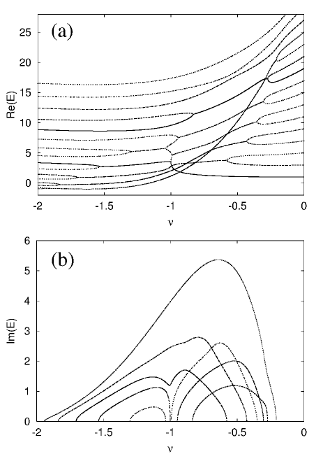
Figure 4: Spectrum for a cut-off length $b=6$.

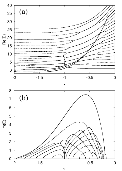
Figure 5: At a cut-off length $b=7$ the generic structure of the spectrum is clearly visible. The web-like pattern of the real components (Fig. 5a) contains purely real branches in the vicinity of the left $(\nu=-2)$ and right $(\nu=0)$ end points of the considered interval as well as a chain of purely real intermediate segments in the vicinity of $\nu=-1$. (See Fig. 6 for a detailed view.) The increasing number of imaginary components (Fig. 5b) with high gradients $|\partial_{\nu}E(\nu\approx-1)|\gg 1$ which accumulate in the vicinity of $\nu=-1$ are first indications of the formation of a local spectral singularity at $\nu=-1$.

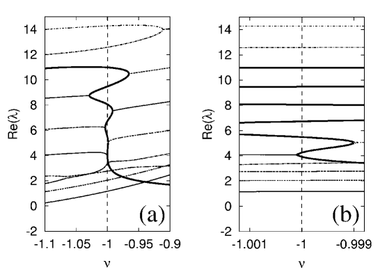
Figure 6: The purely real curve (high-lighted fat) in the vicinity of $\nu=-1$ (cut-off length $b=7$) is formed by intermediate real segments between complex valued segments which branch off to the left and to the right. This leads to a ladder-like structure with exceptional points as nodes. The zoomed picture in Fig. 6b shows that the ”oscillations” of the real curve about the line $\nu=-1$ persist also at its lower end, but with strongly reduced ”amplitude”. When the cut-off is slightly increased to $b\gtrsim 7$ the lowest exceptional (real-to-complex transition) point (Fig. 6b) will cross the line $\nu=-1$ and will in the region $\nu>-1$ coalesce with the other (nearest) exceptional point. As result one intermediate segment will be removed from the real curve and a purely complex-valued branch-pair will smoothly tend from ”far left” $(\nu<-1)$ to ”far right” $(\nu>-1)$ — similar to the lower lying purely complex branches visible in the graphics.

A sample of the results of such a study is depicted in Figures 2 – 6, where we have chosen $g=1$ and displayed the first few energy levels $E(\nu)$ over the entire interval $\nu\in(-2,0)$ for the sequence of values $b=2,4,6,7$. The important results of this numerical experiment are the following:

• At all sufficiently small $b$, as sampled in Fig. 2, the energy spectrum exhibits a more or less $\nu-$independent square-well form.

• At not too large $b$ the spectrum, as sampled in Fig. 3, proves clearly separated into the high-lying part (where the energies still preserve their approximate $\nu-$independence), an intermediate perturbative part (where the perceivably $\nu-$dependent energies still remain all real) and the low-lying part (where one encounters the first real-to-complex phase transitions).

• The actual lowest level numbers $k_{c}(b)$ (critical level numbers) of the modes which are not involved in real-to-complex transitions lie much below the safe supremum bounds $k_{s}(b)$ of inequality (55). Choosing, for example, the exponents $\nu=-1/2$ and $\nu=-3/2$ we read off that

  $$\nu=-1/2: b=\left\{\begin{array}[]{c}2\\ 4\\ 6\\ 7\end{array}\right.,\quad k_{s}(b)>\left\{\begin{array}[]{c}4.08\\ 51.4\\ 213\\ 367\end{array}\right.,\quad k_{c}(b)=\left\{\begin{array}[]{c}1\\ 6\\ 14\\ 22\end{array}\right.,$$ (68)

  $$\nu=-3/2: b=\left\{\begin{array}[]{c}2\\ 4\\ 6\\ 7\end{array}\right.,\quad k_{s}(b)>\left\{\begin{array}[]{c}1.79\\ 12.5\\ 35.2\\ 52.1\end{array}\right.,\quad k_{c}(b)=\left\{\begin{array}[]{c}1\\ 5\\ 9\\ 11\end{array}\right.\,.$$ (81)

• Starting from the “intermediate width” region, sampled at $b=6$ in Fig. 4, we find that the left-hand half of the picture exhibits a clear transition from the slightly non-Hermitian square well regime (with the higher energies all real) to its more strongly non-Hermitian extension where for all exponents $\nu$ not too distant from $\nu=-2$ the purely imaginary and finite component of the potential resembles the spatially antisymmetric part of the exactly solvable ${\cal PT}-$symmetric Heavyside step potential within a square well considered in Ref. [41]. This explains why in Figs. 3 - 5 the continuing decrease of $\nu$ makes the respective two or three lowest pairs of the energies merge and complexify.

• At “sufficiently large” cut-offs $b$, all the real low-lying energies depicted in the right-hand halves of Figs. 4 and 5 obviously stabilize and approach the $b\to\infty$ limiting pattern as published in Ref. [1, 16]. In particular, we see that the ground-state energy remains real and that it starts growing more quickly only when the values of $\nu$ move down and closer to the Herbst limit of $\nu\to-1^{+}$. We observe that in a more appropriate way this growing real branch should be interpreted as a special type of ladder-shaped merger of intermediate real segments which actually correspond to level-pairs with higher mode numbers. A zoomed view on this peculiarity is presented in Fig. 6, where it is clearly visible that a chain of exceptional points is located on this branch with alternating complex-valued segments branching off to the left and to the right. These segments fit, after further complex-to-real transitions, to the real eigenvalues of the $\nu\to 0$ and $\nu\to-2$ limit models.

• When the cut-off $b$ is increased the following simultaneous changes in the spectrum can be observed. In the upper low-energy region with $\nu>-1$ step by step more and more level pairs become twisted into the complex sector. With a ”slight delay in $b$” and at $\nu<-1$ the lower of the twisted levels undergo a second pairwise real-to-complex transition with the levels below them. A sort of web structure is forming with a purely real branch remaining between the left $(\nu<-1)$ and right $(\nu>-1)$ purely complex (twisted) spectral regions. The complex-valued level pairs are branching off from the real branch forming a ladder-shaped structure. At the low-energy end of this ladder a second process occurs. The left $(\nu<-1)$ complex level pairs are passing the line $\nu=-1$ and move to the right of it. There, at some $\nu>-1$ the corresponding exceptional point merges with an exceptional point of a right branch. As result one of the real segments between left and right off-branching levels disappears and a smooth complex-valued branch forms which extends over a large $\nu$ interval and whose imaginary components are increasing very fast when $b$ is increased. It remains the real branch which becomes more and more vertical whereas the complex branch is not intersecting with it (the real component of the complex branch is coinciding at one point with the real branch but the imaginary components are not coinciding).

Analyzing the sequence of Figs. 2 - 6 we observe that, when the cut-off $b$ is increased, a rather special (and seemingly inextricable) branch pattern of real and complex eigenvalues is forming in the vicinity of the exponent $\nu=-1$. The extreme steepness of an increasing number of imaginary branches and their accumulation at $\nu=-1$ (see Figs. 4, 5) as well as the occurrence of the almost vertical real branch (Fig. 6) are indicating the formation of a local spectral singularity with $\left.\partial_{\nu}E\right|_{\nu\to-1}\to\pm\infty$ at the (almost) vertical segments of the real-valued branch as well as on the imaginary branches close to the exceptional points of the ”ladder” structure. From the figures it is not at all obvious how this pattern is compatible with the Herbst limit of an empty spectrum for $b\to\infty$ at $\nu=-1$. We will resolve this interesting puzzle in the next section.

4 The Herbst limit and its relation to the Squire equation of hydrodynamics

In Ref. [15] it was was shown by I. Herbst that the spectrum of a Hamiltonian (82) with imaginary linear potential (imaginary homogeneous electric field) over the real line $x\in{\mathbb{R}}$ is empty. The differential expression of the corresponding operator coincides with that of the ${\cal PT}-$symmetric Schrödinger type equation (51) with exponent $\nu=-1$,

$$\left[-\partial_{y}^{2}-igb^{3}\,y\right]\psi(y)=b^{2}E\,\psi(y),\qquad\psi(y=\pm 1)=0.$$ (82)

The only difference of (82) compared to the Herbst model is in the Dirichlet boundary conditions at $y=\pm 1$ which restrict the system to a box (square well). Due to this analogy and for sake of brevity, we will call the model (82) a ”Herbst box”.

We start our consideration by noticing that Eq. (82) and the spectral function $\mu(b,E)=b^{2}E$ are invariant under the rescaling $b\mapsto g^{-1/3}b,\ E\mapsto g^{2/3}E$ so that henceforth we can set $g=1$, without loss of generality. The corresponding Herbst box Hamiltonian we denote as

$$H_{Hb}(b):=-\partial_{y}^{2}-ib^{3}\,y\,.$$ (83)

Equation (82) itself is of Airy type and its solutions can be expressed as

$$\psi(y) = C_{1}A_{1}[\xi(y)]+C_{2}A_{2}[\xi(y)],$$ (84)

$$\xi(y) := e^{i\frac{\pi}{3}}\left[-iby-E\right],$$ (85)

where $C_{1,2}=\mbox{\rm const}$, and $A_{1}(\xi)$, $A_{2}(\xi)$ are any two of the Airy functions $\mbox{Ai}(\xi),\ \mbox{Ai}(q\xi),\ \mbox{Ai}(q^{2}\xi)$ with $q:=e^{i2\pi/3}$. As usual, the boundary conditions lead to a characteristic determinant which defines the spectrum of the eigenvalue problem. In case of Eq. (82), it reads

$$\Delta(E)=A_{1}(\xi_{+})A_{2}(\xi_{-})-A_{1}(\xi_{-})A_{2}(\xi_{+})=0,\qquad\xi_{\pm}:=\xi(y=\pm 1).$$ (86)

Characteristic determinants of this type (built over Airy functions) have been intensively studied since 1995 in a paper series of Stepin [47, 48] and Shkalikov et al [49] on the spectral properties of the Squire equation of hydrodynamics

$$H_{Sq}(\varepsilon):=i\varepsilon\partial_{y}^{2}+y,\qquad\left(H_{Sq}-\lambda\right)\chi=0,\qquad\chi(y=\pm 1)=0,\qquad\varepsilon:=\left(\tilde{\alpha}R\right)^{-1}.$$ (87)

Before we make the (obviously existing) relation of this model to the Herbst box model explicit, we briefly review a few of its properties.

The Squire equation (87) describes the normal vorticity of a plane Couette flow with linear velocity profile. The parameter $\tilde{\alpha}>0$ denotes a real-valued wave number which originates from the decomposition of a 2D-flow-perturbation

$$\Psi(x,y,t)=\chi(y)e^{i\tilde{\alpha}(x-\lambda t)},$$ (88)

$R>0$ is the Reynolds number and $\varepsilon$ — the viscosity. The spectrum of $H_{Sq}$ was found to have a $Y-$shaped form [48, 49, 51]. All the eigenvalues are located in a close vicinity of the three segments $(1,-i/\sqrt{3}]$, $(-1,-i/\sqrt{3}]$, $[-i/\sqrt{3},-i\infty)$. In the limit of large $R\to\infty$, $\tilde{\alpha}\geq 1$ and correspondingly small $\varepsilon\to 0^{+}$ the eigenvalue problem (87) turns into a singular perturbation problem and its eigenvalues show a remarkable limiting behavior: For $\varepsilon\to 0^{+}$, more and more eigenvalues ”move in” from $-i\infty$ along the line $[-i/\sqrt{3},-i\infty)$, merge pairwise in the vicinity of the point $-i/\sqrt{3}$ and depart then (again pairwise) to move symmetrically along the segments $[1,-i/\sqrt{3}]$, $[-1,-i/\sqrt{3}]$ and to ”fill” them step by step — leaving the $Y$ shape-invariant. The process was described in Ref. [48] as a special type of transition from a discrete spectrum to a continuous one. Explicitly, the following asymptotic estimates were found in [48, 49]

$$\lambda_{n} \sim -i\varepsilon\frac{\pi^{2}n^{2}}{4}\ \in\ [-i/\sqrt{3},-i\infty),\quad n\to\infty$$ (89)

$$\lambda_{n}^{\pm} \sim \pm 1\pm\varepsilon^{1/3}s_{n}\,e^{\pm i\pi/6}\ \in\ (\pm 1,-i/\sqrt{3}],\quad\varepsilon\to 0^{+},$$ (90)

where $s_{n}$ are the zeros of the Airy function

$$\mbox{Ai}(s_{n})=0,\qquad s_{n}\in{\mathbb{R}}_{-}\,.$$ (91)

One clearly sees that the smaller $\varepsilon$ is chosen the smaller the distances between the eigenvalues become — leading in the limit $\varepsilon\to 0$ to a quasi-continuous spectrum.

Noticing that the pairwise merging and splitting (level crossing) of the eigenvalues occurs at $\lambda^{+}\sim\lambda^{-}\sim-i/\sqrt{3}$, it is easy to estimate that the value $\varepsilon_{n}$, for which this crossing is connected with the $n-$th Airy function root $s_{n}$, is given by

$$\varepsilon_{n}^{1/3}\sim\frac{2}{|s_{n}|\sqrt{3}}\ .$$ (92)

Let us utilize the above results now for the Herbst box model. A simple comparison of the eigenvalue problems (82) (for $g=1$) and (87) shows that these problems may be made coinciding if one sets

$$i\varepsilon^{-1}\left[H_{Sq}(\varepsilon)-\lambda\right]\chi(y)\stackrel{{\scriptstyle!}}{{=}}{\cal P}\left[H_{Hb}(b)-b^{2}E\right]{\cal P}\left[{\cal P}\psi(y)\right]=0$$ (93)

and identifies

$$b^{3}=\varepsilon^{-1},\qquad E=ib\lambda,\qquad{\cal P}H_{Hb}(b){\cal P}=i\varepsilon^{-1}H_{Sq}(\varepsilon),\qquad{\cal P}\psi(y)=\chi(y)\,.$$ (94)

This means that the two models are related by the combined action of a rescaling, a Wick-rotation and a coordinate reflection ${\cal P}$.

With the help of the estimates (89), (90) it is now an easy task to explain the behavior of the Herbst-box spectrum $E(b)$.

• The rescaled spectrum $E(b)/b=i\lambda(\varepsilon=b^{-3})$ (shown in Fig. 7) is simply the Wick-rotated version of the original shape-invariant ”Y” of the Squire operator $H_{Sq}(\varepsilon)$.

  

  Figure 7: The rescaled Herbst-box spectrum $E/b=i\lambda(\epsilon=b^{-3})$ coincides with the Wick-rotated $Y-$shaped spectrum of the Squire operator $H_{Sq}(\varepsilon)$.

  With increasing $b=\varepsilon^{-1/3}$ more and more eigenvalues ”move in” from $+\infty$ and ”fill” the two complex conjugate branches $(i,1/\sqrt{3}]$, $(-i,1/\sqrt{3}]$ of the ”Y” as well as the half-line $[1/\sqrt{3},+\infty)$ — in a similar way as in the original $\lambda(\varepsilon\to 0)$ limit. For $b\to\infty$ the spectrum becomes quasi-continuous on the rotated ”Y”.

• Due to the shape invariance of $E(b)/b$, the spectrum $E(b)=ib\lambda(b^{-3})$ itself inflates when $b$ increases. It is located in the close vicinity of the segments $(ib,b/\sqrt{3}]$, $(-ib,b/\sqrt{3}]$, $[b/\sqrt{3},+\infty)$ and moves with $b\to\infty$ to infinity — leaving (for sufficiently high $b$) an empty region at any fixed finite distance from the origin of the spectral $E-$plane. Hence, we find (as required) that for $b\to\infty$ the Herbst box spectrum turns into the empty spectrum of the original Herbst model over the real line ${\mathbb{R}}$.

• For finite $b$, the asymptotic estimates (89), (90) map into

  $$E_{k} \sim \frac{\pi^{2}k^{2}}{4b^{2}}\ \in\ b\times[1/\sqrt{3},+\infty),\quad k\to\infty\,,$$ (95)

  $$E_{n}^{\pm} \sim \pm ib\pm is_{n}\,e^{\pm i\pi/6}\ \in\ b\times(\pm i,1/\sqrt{3}\,],\quad b\to\infty\,,$$ (96)

  and we identify (95) as the pure square well spectrum

  $$\mu(b,E_{k})=b^{2}\,E_{k}\sim\pi^{2}k^{2}/4\ \in\ b^{3}\times[1/\sqrt{3},+\infty)$$ (97)

  of the high-energy sector which is almost not affected by the ${\cal PT}-$symmetric interaction.

  

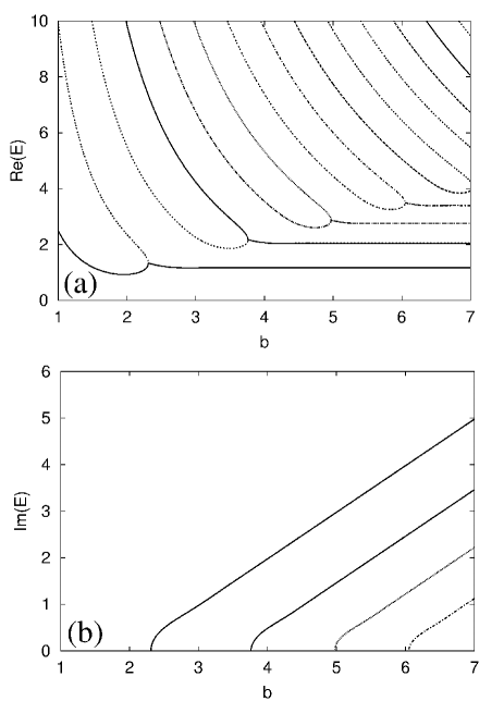
  Figure 8: Real and imaginary components of the Herbst-box spectrum as functions of the cut-off length $b$ (complex conjugate $(\Im\lambda\leq 0)-$components omitted). The asymptotical behavior of the complex-valued branches is clearly visible (constant real components and linear $b-$dependence of the imaginary components).

  In contrast, the low-energy sector described by (96) shows a purely linear scaling behavior of the imaginary energy components $\Im E_{n}^{\pm}$, whereas the real components remain asymptotically fixed when $b$ increases. This situation is also clearly visible from the numerical results presented in Fig. 8.

  

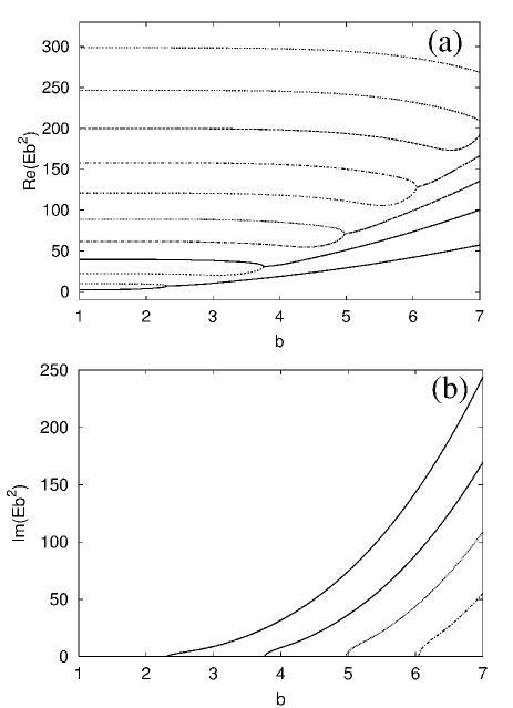
  Figure 9: The rescaled Herbst-box spectrum $\mu(b,E)=b^{2}E$ allows a complementary view on the transition from the high-energy sector to the intermediate and low-energy sector.

  The graphics of the equivalent spectrum $\mu(b,E)$, depicted in Fig. 9, provides a complementary description and shows how (for increasing $b$) the $b-$independent eigenvalues $\mu(b,E_{k})$ of Eq. (97) leave the high-energy sector, obtain an explicit $b-$dependence in the intermediate-energy sector and finally coalesce and split into complex conjugate pairs.

• From the form of the spectral branches on the $E-$plane (rotated ”Y”) it is clear that the level-crossings in the vicinity of $E\sim b/\sqrt{3}$ correspond to the typical real-to-complex phase transitions of ${\cal PT}-$symmetric models in Krein spaces. With the help of relation (92) the cut-off-scales $b_{n}$ and positions $E_{n}$ of the level crossings can be roughly estimated as

  $$b_{n}\sim|s_{n}|\sqrt{3}/2,\qquad E_{n}\sim|s_{n}|/2\,.$$ (98)

  One can use the explicit values of these $b_{n}$, $(b_{1}\approx 2.02,b_{2}\approx 3.54,b_{3}\approx 4.78,b_{4}\approx 5.88,b_{5}\approx 6.87,b_{6}\approx 7.81,\ldots)$, to roughly derive the number of the lowest uncrossed modes in the cases $b=2,4,6,7$. For $b=2,4,6$ the result exactly coincides with the level crossing pattern shown (at $\nu=-1$) in Figs. 2 - 4, whereas the value $b_{5}$ is clearly smaller than the actual transition value $b_{5(c)}$ for which according to Figs. 6b and 8 holds $b_{5(c)}\gtrsim 7$.

  For completeness, we note that the asymptotic approximation [48] of the Airy function roots

  $$|s_{n}|=\left[\frac{3\pi}{2}\left(n-\frac{1}{4}\right)\right]^{2/3}+O(n^{-4/3}),\qquad n\to\infty$$ (99)

  together with (98) yields the following rough estimate for the lowest purely real-valued mode

  $$k_{a}>\frac{4}{3\pi}\left(\frac{2}{\sqrt{3}}\;b\right)^{3/2}+\frac{1}{2}\,.$$ (100)

  The scaling dimension $\kappa_{a}=3/2$ of this bound is only one half of the scaling dimension $\kappa_{s}=4+\nu=3$ of the corresponding supremum bound (55).

  The exact positions of the level crossing points are given by the multiple roots of the characteristic determinant, $\Delta(E)=0$,  $\partial_{E}\Delta(E)=0$. This equation system can be simplified via Wronskian $W[A_{1}(.),A_{2}(.)]$ to yield the conditions

  $$A_{1,2}(\xi_{+})=\pm A_{1,2}(\xi_{-})$$ (101)

  (see [48] for the details).

  Plugging the numerical results from the eigenvalue solver into this equation with $A_{1,2}(\xi)$ chosen as in [48], $A_{1}(\xi):=\mbox{Ai}(\xi)$, $A_{2}(\xi):=\mbox{Ai}(q^{2}\xi)$, selects the condition $A_{1,2}(\xi_{+})=A_{1,2}(\xi_{-})$ and satisfies it within numerical working precision. For the same data holds $A_{1,2}(\xi_{+})\neq-A_{1,2}(\xi_{-})$.

• The spectral behavior $E(b)$ for increasing cut-off $b$ can be summarized as follows. At the beginning, the real eigenvalues from the high-energy sector decrease as $E_{k}\sim\pi^{2}k^{2}/(4b^{2})$ — moving into the intermediate energy region. When $b$ approaches $b_{n}\sim|s_{n}|\sqrt{3}/2$ from below, the real eigenvalues $\{E_{2n-1},E_{2n}\}$  (corresponding to a pair of positive and negative Krein space states [11]) coalesce at $E_{2n-1}\sim E_{2n}\sim|s_{n}|/2$ and a real-to-complex transition occurs $\{E_{2n-1},E_{2n}\}\longrightarrow\{E_{n}^{+},E_{n}^{-}\}$. When $b$ is further increased the real energy components remain fixed $\Re E_{n}^{\pm}\approx|s_{n}|/2$ (see Fig. 8a), whereas the imaginary components blow up linearly along the asymptotes $\Im E_{n}^{\pm}\sim\pm b\pm s_{n}\sqrt{3}/2$ (Fig. 8b).

Let us, for finite $b$, relate the obtained Herbst-box results to the spectral behavior of the ${\cal PT}-$symmetric interpolation model of the previous section. Apart from the obvious one-to-one correspondence of the high-energy sectors (see (97)), a clear identification is immediately possible for those Herbst-box eigenvalues which are close to the imaginary axis and which have the largest imaginary components. These eigenvalues are located on the branches with the largest imaginary components in Figs. 3 - 5 (which stay complex when $\nu$ passes through the Herbst-box value $\nu=-1$). It is clearly visible from these figures that, for increasing $b$, the imaginary components are blowing up, whereas the real components remain asymptotically constant.

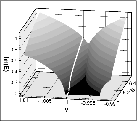
Figure 10: Concrete example for the generic merging process of two complex-valued spectral branches (present here for $b<b_{coal}\approx 6.36$) into a single complex-valued branch for $b>b_{coal}$. The two exceptional (real-to-complex transition) points existing for $b<b_{coal}$ are located on the plane $(\nu,b,\Im E=0)$ and coalesce at $b=b_{coal}$. The corresponding point $(\nu_{coal}\approx-0.9983>-1,b_{coal}\approx 6.36,\Im E=0)$ is the starting (cusp) point of a sharp ”valley” of the non-vanishing imaginary component which steeply grows and smooths when $b>b_{coal}$ is further increased. The white curve marks the Herbst-box values. Before the two exceptional points coalesce, the left one of these points crosses the Herbst-box configuration at $(\nu=-1,b=b_{c}\approx 6.02,\Im E=0)$ and a real-to-complex transition occurs for the Herbst-box model.

So far, we have found a clear correspondence for those regions on the Herbst-box ”Y” which are located away from the center of the ”Y” with its real-to-complex phase transitions. A more subtle situation occurs in the vicinity of this center. The corresponding Herbst box eigenvalues will map into points located close to (or on) the forming (almost) vertical segment of the purely real branch depicted in Fig. 6. From the zoomed graphics in Fig. 6b we observe that the purely real and almost vertical branch of the interpolation model ”oscillates” around the Herbst box line at $\nu=-1$ with strongly decreasing ”amplitude” to its low-energy part. With increasing $b$ this ”decreasing amplitude” effect becomes stronger and the ”oscillations” are only traceable with the help of an appropriately increased zooming scale. Nevertheless, it can be read off that the real-to-complex transition of the Herbst box spectrum follows qualitatively the same scheme for any finite $b$. The real eigenvalues of the Herbst box are all located on the purely real branch of the interpolation model and the real-to-complex transition occurs when the lowest exceptional point on this branch moves from the left sector $\nu<-1$ through the Herbst-box value $\nu=-1$ into the right sector $\nu>-1$ — to coalesce afterwards with the next higher exceptional point from the right sector. With this passing of the left-sector exceptional point through the line $\nu=-1$ the Herbst box eigenvalues become pairwise complex conjugate with strongly increasing imaginary components (due to the asymptotically diverging gradient $\left.\partial_{\nu}E(b\to\infty)\right|_{\nu\approx-1}\longrightarrow\pm\infty$). The real-to-complex transition with subsequently increasing imaginary components are illustrated in Fig. 10.

Finally, we note that in the limit $b\to\infty$, the lowest-lying intersection of the purely real branch with the Herbst-box line $\nu=-1$ moves away to infinity like $b/\sqrt{3}$ (the lower bound of the real segment $[b/\sqrt{3},\infty)$ of the Herbst-box ”Y”) so that the real branch itself remains for any finite energy in the right sector $\nu>-1$ — approaching the Herbst-box line asymptotically. This reproduces the earlier observations of Refs. [1, 16] for the spectrum of the Bender-Boettcher problem over the real line. Additionally, our Herbst box results predict for this problem diverging imaginary components at $\nu=-1$: $|\Im E(b\to\infty,\nu\to-1)|\to\infty$. Taking these observations together we once more see that in the limit $b\to\infty$ a spectral singularity is forming at $\nu=-1$ with $|E(b\to\infty,\nu\to-1)|\to\infty$, $|\partial_{\nu}E(b\to\infty,\nu\to-1)|\to\infty$.

5 Conlusions

In the present paper we considered three models emerging in different physical setups, but which are closely related with each other by their underlying mathematical structure as spectral problems in Krein spaces. The models are a one-dimensional ${\cal PT}-$symmetric quantum mechanical interpolation setup defined over a square well of finite width $2b$, the spherically symmetric MHD $\alpha^{2}-$dynamo as well as the Squire equation of hydrodynamics. For the PTSQM model and the $\alpha^{2}-$dynamo we made their close relation transparent by transforming them into a $2\times 2$ matrix operator representation with coinciding block structure of the Krein space metric (involution operator). In the case of the Squire equation we showed that the corresponding spectral problem is connected with a ${\cal PT}-$symmetric eigenvalue problem by a rescaling and Wick rotation.

Based on recent results on the spectrum of the Squire equation, we performed a qualitative analysis of the ${\cal PT}-$symmetric quantum mechanical interpolation model for arbitrary square well widths (cut-offs) $2b$. This allowed us to trace the emergence of the Herbst limit with its empty spectrum as a spectral singularity and to fit our results to those of the Bender-Boettcher equation over the real line. We obtained a rich structure of multiple spectral phase transitions from purely real eigenvalues to pairs of complex conjugate ones — as it was to expect for spectral problems in Krein spaces.

A deeper insight into the Herbst-box spectrum and a possible extension of the present results to ${\cal PT}-$symmetric Hamiltonians of the type $H_{M,N}=-\partial_{x}^{2}+x^{2M}(ix)^{N},\ M,N=1,2,3,\ldots$ over square wells can probably be achieved by representing the characteristic determinant $\Delta(E)$ in (86) via Hadamar product representation of the Airy functions [53] as a spectral determinant of Bethe-ansatz type [16, 29, 54] and studying it by similar cocycle functional equations as in Ref. [55].

A question which was not touched in the present paper concerns the orthogonality of the Herbst-box eigenfunctions. For the Squire equation it is known that its eigenfunctions show a strong non-orthogonality [47, 51] (due to the non-normality of the Squire operator) for eigenvalues in the vicinity of the branch point center of the ”Y” (pseudo-spectral techniques [50, 51, 56] play an important role in this case). Our above considerations indicate on a link of this issue with the forming spectral singularity $|\partial_{\nu}E(\nu\approx-1,b\gg 1)|\gg 1$ in the vicinity of the almost vertical segments of the purely real branch in the spectrum of the ${\cal PT}-$symmetric interpolation model.

Finally, we would like to note two issues which seem of relevance for future considerations. The first one is in developing efficient mathematical tools to find the hyper-surfaces in parameter space where spectral phase transitions of the real-to-complex type occur. Knowing these hyper-surfaces, one would know the boundaries which separate the parameter space regions with unbroken ${\cal PT}-$symmetry from regions with spontaneously broken ${\cal PT}-$symmetry. In case of $\alpha^{2}-$dynamos the corresponding knowledge would allow for a more precise prediction of configurations with tendency to magnetic field reversals. The second issue concerns methods for solving inverse spectral problems in Krein spaces. Such methods would be extremely helpful for the data analysis of the dynamo experiments which are planned for the near future at seven sites around the world [58].

Appendix A A few comments on the physics of MHD $\alpha^{2}-$dynamos

The dynamo operator $\hat{H}_{l}[\alpha]$ originates from the MHD mean-field induction equation (cf. [12])

$$\partial_{t}\mathbf{B}=\boldsymbol{\nabla\times}(\alpha\mathbf{B})+\nu_{m}\Delta\mathbf{B}$$ (102)

for the magnetic field $\mathbf{B}$. This equation results from averaging over small scale turbulences in the velocity field of the electrically conducting fluid (or plasma) which drives the dynamo. The helical turbulence function $\alpha(x)$ (also called $\alpha-$profile) encodes the net effect of the small scale physics on the large scale (mean) magnetic field $\mathbf{B}$. For certain topologically non-trivial helical velocity and $\mathbf{B}-$field configurations an inverse cascade effect occurs which induces an energy transfer from small-scale structures to large-scale structures (inverse to the energy transfer in usual turbulence cascades where the energy is pumped from large-scale structures into smaller structures until it finally dissipates and transforms into thermal energy). For sufficiently strong inverse cascade effects the advection term $\boldsymbol{\nabla\times}(\alpha\mathbf{B})$ starts to dominate over the diffusion term $\nu_{m}\Delta\mathbf{B}$ ($\nu_{m}$ is the magnetic diffusivity) and the magnetic field strength starts to grow exponentially. This kinematic dynamo effect (growing $\mathbf{B}-$field for a given velocity field of the fluid) is followed by a saturated dynamo regime where a balance between the dynamo effect and the back-reaction of the induced magnetic field on the velocity field (via Navier-Stokes equation) prevents a further growth of the field strength $\mathbf{B}$. For completeness, we note that an MHD dynamo is an open system in which part of the kinetic energy of the conducting fluid (or plasma) transforms into magnetic field energy.

The dynamo eigenvalue problem

$$\hat{H}_{l}[\alpha]\phi_{l,n}=\lambda_{l,n}\phi_{l,n},\qquad\phi_{l,n}(t)\sim\exp\lambda_{l,n}\,t$$ (103)

follows from the induction equation (102) via a double decomposition: decomposing the $\mathbf{B}-$field into poloidal and toroidal components (what leads to the two-component vector structure of $\phi_{l,n}$) and expanding them further into spherical harmonics. In the simplest (toy model) case of a spherically symmetric dynamo configuration the corresponding modes decouple completely and one arrives at the spherical $l-$mode projection (25), (103) (the subscript $n$ denotes the radial mode number).

Up to now only a single exactly solvable $\alpha^{2}-$dynamo model is known — the model with constant $\alpha-$profile [12]. Its spectrum is discrete, real [59], bounded above and, depending on the value of $\alpha$, it is either completely negative (for $\alpha$ below a critical $\alpha_{c}:\ \alpha<\alpha_{c}$) or it contains a finite number of positive eigenvalues $\lambda_{l,n}>0$. The dynamo effect is dominated by these latter eigenmodes. In practice, it usually suffices to concentrate the analysis on the dominating upper most growing mode (or a few of the upper most modes) for dipole (l=1) and quadrupole (l=2) configurations. (There exist no “$s-$wave” $\alpha^{2}-$dynamos with $l=0$ [12, 13].)

The spectral properties of the dynamo operator $\hat{H}_{l}[\alpha]$ are becoming much richer for inhomogeneous $\alpha-$profiles $\alpha(r)\neq\mbox{\rm const}$, when real-to-complex transitions occur — as discussed in Subsection 2.3 and shown in Fig. 1.

References

- [1] C. M. Bender and S. Boettcher, Phys. Rev. Lett. 24, 5243 (1998), physics/9712001.
- [2] C. M. Bender, S. Boettcher and P. N. Meisinger, J. Math. Phys. 40, 2201 (1999), quant-ph/9809072.
- [3] M. Znojil, Phys. Lett. A259, 220 (1999), quant-ph/9905020; M. Znojil, J. Phys. A 33 4203 (2000), math-ph/0002036; M. Znojil, F. Cannata, B. Bagchi, and R. Roychoudhury, Phys. Lett. B483, 284 (2000), hep-th/0003277.
- [4] A. Mostafazadeh, J. Math. Phys. 43, 205 (2002), math-ph/0107001; ibid. 43, 2814 (2002), math-ph/0110016.
- [5] A. Mostafazadeh, J. Math. Phys. 43, 3944 (2002), math-ph/0203005.
- [6] C. M. Bender, D. C. Brody and H. F. Jones, Phys. Rev. Lett. 89, 270401 (2002), quant-ph/0208076.
- [7] C. M. Bender, D. C. Brody and H. F. Jones, Am. J. Phys. 71, 1095 (2003), hep-th/0303005.
- [8] C. M. Bender, Czech. J. Phys. 54, 13 (2004); ibid. 54, 1027 (2004).
- [9] T. Ya. Azizov and I. S. Iokhvidov, Linear operators in spaces with an indefinite metric (Wiley-Interscience, New York, 1989).
- [10] A. Dijksma and H. Langer, Operator theory and ordinary differential operators, in A. Böttcher (ed.) et al., Lectures on operator theory and its applications, Providence, RI: Am. Math. Soc., Fields Institute Monographs, Vol. 3, 75 (1996).
- [11] H. Langer and C. Tretter, Czech. J. Phys. 54, 1113 (2004).
- [12] H. K. Moffatt, Magnetic field generation in electrically conducting fluids (Cambridge University Press, Cambridge, 1978); F. Krause and K.-H. Rädler, Mean-field magnetohydrodynamics and dynamo theory (Akademie-Verlag, Berlin and Pergamon Press, Oxford, 1980); Ya. B. Zeldovich, A. A. Ruzmaikin, and D. D. Sokoloff, Magnetic fields in astrophysics (Gordon & Breach Science Publishers, New York, 1983).
- [13] U. Günther and F. Stefani, J. Math. Phys. 44, 3097 (2003), math-ph/0208012.
- [14] U. Günther, F. Stefani and G. Gerbeth, Czech. J. Phys. 54, 1075 (2004), math-ph/0407015.
- [15] I. Herbst, Commun. Math. Phys. 64, 279 (1977).
- [16] P. Dorey, C. Dunning and R. Tateo, J. Phys. A 34, 5679 (2001), hep-th/0103051.
- [17] C. M. Bender, Introduction to PT-symmetric quantum theory, to be published in Contemporary Physics, quant-ph/0501052.
- [18] M. Znojil, What is PT symmetry?, quant-ph/0103054v1.
- [19] G. S. Japaridze, J. Phys. A 35, 1709 (2002), quant-ph/0104077.
- [20] A. Messiah, Quantum Mechanics (North Holland, Amsterdam, 1961).
- [21] A. Mostafazadeh, Nucl. Phys. B640, 419 (2002), math-ph/0203041.
- [22] C. M. Bender, P. N. Meisinger and Q. Wang, J. Phys. A 36, 6791 (2003), quant-ph/0303174.
- [23] A. Mostafazadeh, J. Phys. A 36, 7081 (2003), quant-ph/0304080.
- [24] M. R. E. Proctor, Astron. Nachr. 298, 19 (1977); Geophys. Astrophys. Fluid Dyn. 8, 311 (1977); K.-H. Rädler, Geophys. Astrophys. Fluid Dyn. 20, 191 (1982); K.-H. Rädler and U. Geppert, Turbulent dynamo action in the high-conductivity limit: a hidden dynamo, in: M. Nunez and A. Ferriz-Mas (eds.), Workshop on stellar dynamos, ASP Conference Series 178, 151 (1999).
- [25] A. de Souza Dutra and C. A. S. Almeida, Phys. Lett. A275, 25 (2000), quant-ph/0306065; B. Bagchi, P. Gorain, C. Quesne, and R. Roychoudhury, Mod. Phys. Lett. A19, 2765 (2004), quant-ph/0405193; Czech. J. Phys. 54, 1019 (2004).
- [26] F. Kleefeld, Non-Hermitian quantum theory and its holomorphic representation: Introduction and some applications, hep-th/0408028; Non-Hermitian quantum theory and its holomorphic representation: Introduction and applications, (invited contribution to the 2nd International Workshop on ”Pseudo-Hermitian Hamiltonians in Quantum Physics”, Prague, Czech Republic, June 14-16, 2004), hep-th/0408097.
- [27] A. Mostafazadeh, J. Math. Phys. 43, 6343 (2002); Erratum-ibid. 44, 943 (2003), math-ph/0207009.
- [28] C. Dembowski et al, Phys. Rev. Lett. 86, 787 (2001); W. D. Heiss and H. L. Harney, Eur. Phys. J. D17, 149 (2001), quant-ph/0012093.
- [29] K. C. Shin, Commun. Math. Phys. 229 543 (2002), math-ph/0201013.
- [30] F. Stefani and G. Gerbeth, Asymmetric polarity reversals, bimodal field distribution, and coherence resonance in a spherically symmetric mean-field dynamo model, physics/0411050.
- [31] R. T. Merill, M. W. McElhinny and P. L. McFadden, The Magnetic Field of the Earth (Academic Press, San Diego, 1996).
- [32] E. Covas, R. Tavakol, A. Tworkowski, and A. Brandenburg, Astron. Astrophys. 329, 350 (1998), astro-ph/9709062; G. Rüdiger and R. Hollerbach, The magnetic Universe (Wiley-VCH, Weinheim, 2004), p. 160.
- [33] C. M. Bender and T. T. Wu, Phys. Rev. 184, 1231 (1969).
- [34] W.D. Heiss and W.H. Steeb, J. Math. Phys. 32, 3003 (1991).
- [35] F. Stefani and G. Gerbeth, Phys. Rev. E67, 027302 (2003), astro-ph/0210412.
- [36] T. Kato, Perturbation theory for linear operators (Springer, Berlin, 1966).
- [37] M. V. Berry, Czech. J. Phys. 54, 1039 (2004).
- [38] W. D. Heiss: Czech. J. Phys. 54, 1091 (2004).
- [39] M.V. Berry and M. Wilkinson: Proc. R. Soc. Lond. A392, 15 (1984).
- [40] A. Marshakov: Seiberg-Witten theory and integrable systems (World Scientific, Singapore, 1999).
- [41] M. Znojil, Phys. Lett. A285, 7 (2001), quant-ph/0101131; M. Znojil and G. Lévai, Mod. Phys. Lett. A16, 2273 (2001), hep-th/0111213; M. Znojil, J. Math. Phys. 45, 4418 (2004), math-ph/0403033; A. Mostafazadeh and A. Batal, J. Phys. A 37, 11645 (2004), quant-ph/0408132; .
- [42] B. Bagchi, S. Mallik and C. Quesne, Mod. Phys. Lett. A17, 1651 (2002), quant-ph/0205003; V. Jakubský and M. Znojil, Czech. J. Phys. 54, 1101 (2004); M. Znojil, Solvable PT-symmetric model with a tunable interspersion of non-merging levels, quant-ph/0410196.
- [43] M. Reed and B. Simon, Methods of modern mathematical physics, Vol. 1. Functional analysis (Academic Press, New York, 1972).
- [44] C. Tretter, private communication.
- [45] W.H. Press, S.A. Teukolsky, W.T. Vetterling, and B.F. Flannery, Numerical Recipes (Cambridge University Press, Cambridge, 1992).
- [46] F. M. Fernandez, R. Guardiola, J. Ros, and M. Znojil, J. Phys. A 32, 3105 (1999), quant-ph/9812026.
- [47] S. A. Stepin, Usp. Mat. Nauk 50, No.6, 219 (1995), [Russ. Math. Surv. 50, No.6, 1311 (1995)]; Usp. Mat. Nauk 53, No.3, 205 (1998), [Russ. Math. Surv. 53, No.3, 639 (1998)].
- [48] S. A. Stepin, Fundam. Prikl. Mat. 3, No.4, 1199 (1997), (Fundamental and Applied Mathematics), (in Russian), freely available under: http://www.emis.de/journals/FPM/eng/econtent.htm.
- [49] A. A. Shkalikov, Mat. Zametki 62, 950 (1997), [Math. Notes 62, 796 (1997)]; A. A. Shkalikov and S. N. Tumanov, Mat. Zametki 72, 561 (2002), [Math. Notes 72, 519 (2002)]; A. V. Dyachenko and A. A. Shkalikov, Funkts. Anal. Prilozh. 36, No.3, 71 (2002), [Funct. Anal. Appl. 36, 228 (2002)], math.FA/0212127; A. A. Shkalikov, Spectral portraits of the Orr–Sommerfeld operator with large Reynolds numbers, math-ph/0304030.
- [50] P. Redparth, J. Differ. Equations 177, 307 (2001), math.SP/0003044.
- [51] S. C. Reddy, P. J. Schmid and D. S. Henningson, SIAM J. Appl. Math. 53, 15 (1993).
- [52] P. J. Schmid and D. S. Henningson, Stability and transition in shear flows (Springer, New York, 2001).
- [53] E. P. Merkes and M. Salmassi, Complex Variables, Theory Appl. 33, 207 (1997); M. Salmassi, J. Math. Anal. Appl. 240, 574 (1999).
- [54] P. Dorey and R. Tateo, J. Phys. A 32, L419 (1999), hep-th/9812211; P. Dorey, A. Millican-Slater and R. Tateo, Beyond the WKB approximation in PT-symmetric quantum mechanics, hep-th/0410013; P. Dorey, C. Dunning and R. Tateo, Aspects of the ODE/IM correspondence, hep-th/0411069.
- [55] A. Voros, J. Phys. A 32, 1301 (1999), math-ph/9811001; J. Phys. A 32, 5993 (1999), [corrigendum ibid. A 33, 5783 (2000)], math-ph/9903045.
- [56] L. N. Trefethen, A. E. Trefethen, S. C. Reddy, and T. A. Driscoll, Science 261, 578 (1993); S. C. Reddy and L. N. Trefethen, SIAM J. Appl. Math. 54, 1634 (1994); E. B. Davies, Commun. Math. Phys. 200, 35 (1999), math.SP/9803129; A. Aslanyan and E. B. Davies, Numer. Math. 85, 525 (2000), math.SP/9810063; M. Zworski, Commun. Math. Phys. 229, 293 (2002).
- [57] U. Günther, P. Moniz and A. Zhuk, Phys. Rev. D68, 044010 (2003), hep-th/0303023; U. Günther, A. Zhuk, V. Bezerra, and C. Romero, AdS and stabilized extra dimensions in multidimensional gravitational models with nonlinear scalar curvature terms and , hep-th/0409112.
- [58] A. Gailitis et al., Phys. Rev. Lett. 84, 4365 (2000); ibid. 86, 3024 (2001), physics/0010047; U. Müller and R. Stieglitz, Phys. Fluids 13, 561 (2001); A. Gailitis et al., Rev. Mod. Phys. 74, 973 (2002).
- [59] K.-H. Rädler and H.-J. Bräuer, Astron. Nachr. 308, 101 (1987).