Numerical Methods for Eigenvalue Distributions of Random Matrices

Abstract

We present efficient numerical techniques for calculation of eigenvalue distributions of random matrices in the beta-ensembles. We compute histograms using direct simulations on very large matrices, by using tridiagonal matrices with appropriate simplifications. The distributions are also obtained by numerical solution of the Painlevé II and V equations with high accuracy. For the spacings we show a technique based on the Prolate matrix and Richardson extrapolation, and we compare the distributions with the zeros of the Riemann zeta function.

1 Largest Eigenvalue Distributions

In this section, the distributions of the largest eigenvalue of matrices in the $\beta$-ensembles are studied. Histograms are created first by simulation, then by solving the Painlevé II nonlinear differential equation.

1.1 Simulation

The Gaussian Unitary Ensemble (GUE) is defined as the Hermitian $n\times n$ matrices $A$, where the diagonal elements $x_{jj}$ and the upper triangular elements $x_{jk}=u_{jk}+iv_{jk}$ are independent Gaussians with zero-mean, and

$$\begin{cases}\mathrm{Var}(x_{jj})=1,&1\leq j\leq n,\\ \mathrm{Var}(u_{jk})=\mathrm{Var}(v_{jk})=\frac{1}{2},&1\leq j<k\leq n.\end{cases}$$ (1)

Since a sum of Gaussians is a new Gaussian, an instance of these matrices can be created conveniently in MATLAB:

  A=randn(n)+i*randn(n);
  A=(A+A’)/2;

The largest eigenvalue of this matrix is about $2\sqrt{n}$. To get a distribution that converges as $n\rightarrow\infty$, the shifted and scaled largest eigenvalue $\lambda_{\mathrm{max}}^{\prime}$ is calculated as

$$\lambda_{\mathrm{max}}^{\prime}=n^{\frac{1}{6}}\left(\lambda_{\mathrm{max}}-2\sqrt{n}\right).$$ (2)

It is now straight-forward to compute the distribution for $\lambda_{\mathrm{max}}^{\prime}$ by simulation:

  for ii=1:trials
    A=randn(n)+i*randn(n);
    A=(A+A’)/2;
    lmax=max(eig(A));
    lmaxscaled=n^(1/6)*(lmax-2*sqrt(n));
    % Store lmax
  end

  % Create and plot histogram

The problem with this technique is that the computational requirements and the memory requirements grow fast with $n$, which should be as large as possible in order to be a good approximation of infinity. Just storing the matrix $A$ requires $n^{2}$ double-precision numbers, so on most computers today $n$ has to be less than $10^{4}$. Furthermore, computing all the eigenvalues of a full Hermitian matrix requires a computing time proportional to $n^{3}$. This means that it will take many days to create a smooth histogram by simulation, even for relatively small values of $n$.

To improve upon this situation, another matrix can be studied that has the same eigenvalue distribution as $A$ above. In [2], it was shown that this is true for the following symmetric matrix when $\beta=2$:

$$H_{\beta}\sim\frac{1}{\sqrt{2}}\begin{pmatrix}N(0,2)&\chi_{(n-1)\beta}&&&\\ \chi_{(n-1)\beta}&N(0,2)&\chi_{(n-2)\beta}&&\\ &\ddots&\ddots&\ddots&\\ &&\chi_{2\beta}&N(0,2)&\chi_{\beta}\\ &&&\chi_{\beta}&N(0,2)\end{pmatrix}.$$ (3)

Here, $N(0,2)$ is a zero-mean Gaussian with variance $2$, and $\chi_{d}$ is the square-root of a $\chi^{2}$ distributed number with $d$ degrees of freedom. Note that the matrix is symmetric, so the subdiagonal and the superdiagonal are always equal.

This matrix has a tridiagonal sparsity structure, and only $2n$ double-precision numbers are required to store an instance of it. The time for computing the largest eigenvalue is proportional to $n$, either using Krylov subspace based methods or the method of bisection [7].

In MATLAB, the built-in function eigs can be used, although that requires dealing with the sparse matrix structure. There is also a large amount of overhead in this function, which results in a relatively poor performance. Instead, the function maxeig is used below to compute the eigenvalues. This is not a built-in function in MATLAB, but it can be downloaded from http://www-math.mit.edu/$\sim$persson/mltrid. It is based on the method of bisection, and requires just two ordinary MATLAB vectors as input, corresponding to the diagonal and the subdiagonal.

It also turns out that only the first $10n^{\frac{1}{3}}$ components of the eigenvector corresponding to the largest eigenvalue are significantly greater than zero. Therefore, the upper-left $n_{\mathrm{cutoff}}$ by $n_{\mathrm{cutoff}}$ submatrix has the same largest eigenvalue (or at least very close), where

$$n_{\mathrm{cutoff}}\approx 10n^{\frac{1}{3}}.$$ (4)

Matrices of size $n=10^{12}$ can then easily be used since the computations can be done on a matrix of size only $10n^{\frac{1}{3}}=10^{5}$. Also, for these large values of $n$ the approximation $\chi^{2}_{n}\approx n$ is accurate.

A histogram of the distribution for $n=10^{9}$ can now be created using the code below.

  n=1e9;
  nrep=1e4;
  beta=2;

  cutoff=round(10*n^(1/3));
  d1=sqrt(n-1:-1:n+1-cutoff)’/2/sqrt(n);

  ls=zeros(1,nrep);
  for ii=1:nrep
    d0=randn(cutoff,1)/sqrt(n*beta);
    ls(ii)=maxeig(d0,d1);
  end

  ls=(ls-1)*n^(2/3)*2;

  histdistr(ls,-7:0.2:3)

where the function histdistr below is used to histogram the data. It assumes that the histogram boxes are equidistant.

  function [xmid,H]=histdistr(ls,x)

  dx=x(2)-x(1);
  H=histc(ls,x);
  H=H(1:end-1);
  H=H/sum(H)/dx;
  xmid=(x(1:end-1)+x(2:end))/2;

  bar(xmid,H)
  grid on

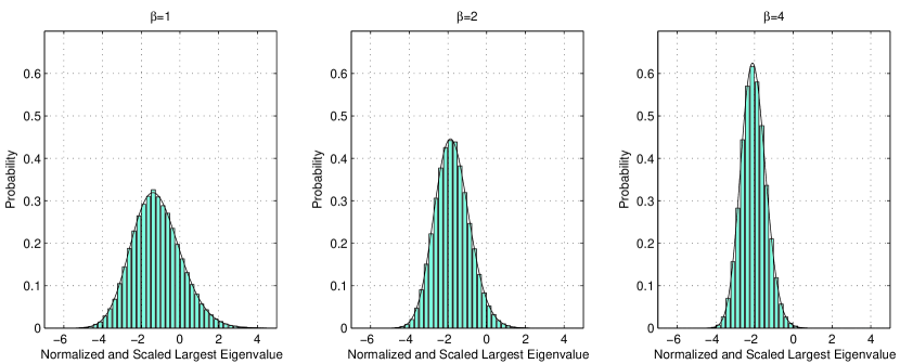
The resulting distribution is shown in Figure 1, together with distributions for $\beta=1$ and $\beta=4$. The plots also contain solid curves representing the “true solutions” (see next section).

Figure 1: Probability distribution of scaled largest eigenvalue ($10^{5}$ repetitions, $n=10^{9}$)

1.2 Painlevé II

Instead of using simulation to plot the distributions of the largest eigenvalues, it can be computed from the solution of the Painlevé II nonlinear differential equation [6]:

$$q^{\prime\prime}=sq+2q^{3}$$ (5)

with the boundary condition

$$q(s)\sim\mathrm{Ai}(s),\qquad\textrm{as }s\rightarrow\infty.$$ (6)

The probability distribution $f_{2}(s)$, corresponding to $\beta=2$, is then given by

$$f_{2}(s)=\frac{d}{ds}F_{2}(s),$$ (7)

where

$$F_{2}(s)=\exp\left(-\int_{s}^{\infty}(x-s)q(x)^{2}\,dx\right).$$ (8)

The distributions for $\beta=1$ and $\beta=4$ are the derivatives of

$$F_{1}(s)^{2} =F_{2}(s)e^{-\int_{s}^{\infty}q(x)\,dx}$$ (9)

and

$$F_{4}\left(\frac{s}{2^{\frac{2}{3}}}\right)^{2} =F_{2}(s)\left(\frac{e^{\frac{1}{2}\int_{s}^{\infty}q(x)\,dx}+e^{-\frac{1}{2}\int_{s}^{\infty}q(x)\,dx}}{2}\right)^{2}.$$ (10)

To solve this numerically using MATLAB, first rewrite (5) as a first-order system:

$$\frac{d}{ds}\begin{pmatrix}q\\ q^{\prime}\end{pmatrix}=\begin{pmatrix}q^{\prime}\\ sq+2q^{3}\end{pmatrix}.$$ (11)

This can be solved as an initial-value problem starting at $s=s_{0}=$ sufficiently large positive number, and integrating along the negative $s$-axis. The boundary condition (6) then becomes the initial values

$$\left\{\begin{array}[]{rcl}q(s_{0})&=&\mathrm{Ai}(s_{0})\\ q^{\prime}(s_{0})&=&\mathrm{Ai}^{\prime}(s_{0}).\end{array}\right.$$ (14)

Although the distributions can be computed from $q(s)$ as a post-processing step, it is most convenient to add a few variables and equations to the ODE system. When computing $F_{2}(s)$, the quantity $I(s)=\int_{s}^{\infty}(x-s)q(x)^{2}\,dx$ is required. Differentiate this twice to get

$$I^{\prime}(s) =-\int_{s}^{\infty}q(x)^{2}\,dx$$ (15)

and

$$I^{\prime\prime}(s) =q(s)^{2}.$$ (16)

Add these equations and the variables $I(s),I^{\prime}(s)$ to the ODE system, and the solver will do the integration. This is not only easier and gives less code, it will also give a much more accurate solution since the same tolerance requirements are imposed on $I(s)$ as on the solution $q(s)$.

In a similar way, the quantity $J(s)=\int_{s}^{\infty}q(x)\,dx$ is needed when computing $F_{1}(s)$ and $F_{4}(s)$. This is handled by adding the variable $J(s)$ and the equation $J^{\prime}(s)=-q(s)$.

The final system now has the form

$$\frac{d}{ds}\begin{pmatrix}q\\ q^{\prime}\\ I\\ I^{\prime}\\ J\end{pmatrix}=\begin{pmatrix}q^{\prime}\\ sq+2q^{3}\\ I^{\prime}\\ q^{2}\\ -q\end{pmatrix}$$ (17)

with the initial condition

$$\begin{pmatrix}q(s_{0})\\ q^{\prime}(s_{0})\\ I(s_{0})\\ I^{\prime}(s_{0})\\ J(s_{0})\end{pmatrix}=\begin{pmatrix}\mathrm{Ai}(s_{0})\\ \mathrm{Ai}^{\prime}(s_{0})\\ \int_{s_{0}}^{\infty}(x-s_{0})\mathrm{Ai}(x)^{2}\,dx\\ \mathrm{Ai}(s_{0})^{2}\\ \int_{s_{0}}^{\infty}\mathrm{Ai}(x)\,dx\end{pmatrix}.$$ (18)

This problem can be solved in just a few lines of MATLAB code using the built-in Runge-Kutta based ODE solver ode45. First define the system of equations as an inline function

  deq=inline(’[y(2); s*y(1)+2*y(1)^3; y(4); y(1)^2; -y(1)]’,’s’,’y’);

Next specify the integration interval and the desired output times.

  s0=5;
  sn=-8;
  sspan=linspace(s0,sn,1000);

The initial values can be computed as

  y0=[airy(s0); airy(1,s0); ...
      quadl(inline(’(x-s0).*airy(x).^2’,’x’,’s0’),s0,20,1e-25,0,s0); ...
      airy(s0)^2; quadl(inline(’airy(x)’),s0,20,1e-18)];

where the quadl function is used to numerically approximate the integrals in (18). Now, the integration tolerances can be set and the system integrated:

  opts=odeset(’reltol’,1e-13,’abstol’,1e-15);
  [s,y]=ode45(deq,sspan,y0,opts);

The five dependent variables are now in the columns of the MATLAB variable y. Using these, $F_{2}(s),F_{1}(s)$, and $F_{4}(s)$ become

  F2=exp(-y(:,3));
  F1=sqrt(F2.*exp(-y(:,5)));
  F4=sqrt(F2).*(exp(y(:,5)/2)+exp(-y(:,5)/2))/2;
  s4=s/2^(2/3);

The probability distributions $f_{2}(s),f_{1}(s)$, and $f_{4}(s)$ could be computed by numerical differentiation:

  f2=gradient(F2,s);
  f1=gradient(F1,s);
  f4=gradient(F4,s4);

but it is more accurate to first do the differentiation symbolically:

$$f_{2}(s) =-I^{\prime}(s)F_{2}(s)$$ (19)

$$f_{1}(s) =\frac{1}{2F_{1}(s)}\left(f_{2}(s)+q(s)F_{2}(s)\right)e^{-J(s)}$$ (20)

$$f_{4}(s) =\frac{1}{2^{\frac{1}{3}}4F_{4}(s)}\left(f_{2}(s)\left(2+e^{J(s)}+e^{-J(s)}\right)+F_{2}(s)q(s)\left(e^{-J(s)}-e^{J(s)}\right)\right)$$ (21)

and evaluate these expressions:

  f2=-y(:,4).*F2;
  f1=1/2./F1.*(f2+y(:,1).*F2).*exp(-y(:,5));
  f4=1/2^(1/3)/4./F4.*(f2.*(2+exp(y(:,5))+exp(-y(:,5)))+ ...
                       F2.*y(:,1).*(exp(-y(:,5))-exp(y(:,5))));

Finally, plot the curves:

  plot(s,f1,s,f2,s4,f4)
  legend(’\beta=1’,’\beta=2’,’\beta=4’)
  xlabel(’s’)
  ylabel(’f_\beta(s)’,’rotation’,0)
  grid on

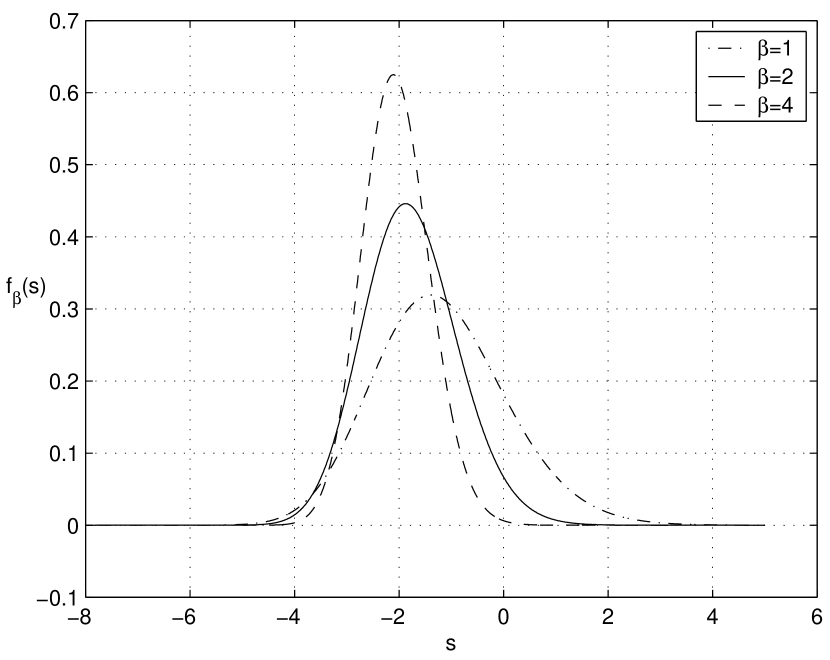
The result can be seen in Figure 2.

Figure 2: The probability distributions $f_{1}(s)$, $f_{2}(s)$, and $f_{4}(s)$, computed using the Painlevé II solution.

2 Eigenvalue Spacings Distributions

Another quantity with an interesting probability distribution is the spacings of the eigenvalues of random matrices. It turns out that the eigenvalues are almost uniformly distributed, which means that every random matrix gives a large number of spacings. The distributions can then be efficiently computed by simulation.

Two other methods are used to compute the spacings distribution – the solution of the Painlevé V nonlinear differential equation and the eigenvalues of the Prolate matrix. Finally, the results are compared with the spacings of the zeros along the critical line of the Riemann zeta function.

2.1 Simulation

As before, the simulations are made with matrices from the Gaussian Unitary Ensemble. The normalized spacings of the eigenvalues $\lambda_{1}\leq\lambda_{2}\leq\ldots\leq\lambda_{N}$ are computed according to

$$\delta^{\prime}_{k}=\frac{\lambda_{k+1}-\lambda_{k}}{\pi\beta}\sqrt{2\beta n-\lambda_{k}^{2}},\qquad k\approx n/2,$$ (22)

where $\beta=2$ for the GUE. The distribution of the eigenvalues is almost uniform, with a slight deviation at the two ends of the spectrum. Therefore, only half of the eigenvalues are used, and one quarter of the eigenvalues at each end is discarded.

Again, to allow for a more efficient simulation, the tridiagonal matrix (3) is used instead of the full Hermitian matrix. In this case, all the eigenvalues are computed, which can be done in a time proportional to $n^{2}$. While this could in principle be done using the MATLAB sparse matrix structure and the eigs function, the more efficient trideig function is used below to compute all the eigenvalues of a symmetric tridiagonal matrix. It can be downloaded from http://www-math.mit.edu/$\sim$persson/mltrid.

The histogram can now be computed by simulation with the following lines of code. Note that the function chi2rnd from the Statistics Toolbox is required.

  n=1000;
  nrep=1000;
  beta=2;

  ds=zeros(1,nrep*n/2);
  for ii=1:nrep
    l=trideig(randn(n,1),sqrt(chi2rnd((n-1:-1:1)’*beta)/2));
    d=diff(l(n/4:3*n/4))/beta/pi.*sqrt(2*beta*n-l(n/4:3*n/4-1).^2);
    ds((ii-1)*n/2+1:ii*n/2)=d;
  end

  histdistr(ds,0:0.05:5);

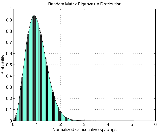
The resulting histogram can be found in Figure 3. The figure also shows the expected curve as a solid line.

Figure 3: Probability distribution of consecutive spacings of random matrix eigenvalues ($1000$ repetitions, $n=1000$)

2.2 Painlevé V

The probability distribution $p(s)$ for the eigenvalue spacings when $\beta=2$ can be computed with the solution to the Painlevé V nonlinear differential equation (see [5] for details):

$$(t\sigma^{\prime\prime})^{2}+4(t\sigma^{\prime}-\sigma)\left(t\sigma^{\prime}-\sigma+(\sigma^{\prime})^{2}\right)=0$$ (23)

with the boundary condition

$$\sigma(t)\approx-\frac{t}{\pi}-\left(\frac{t}{\pi}\right)^{2},\qquad\textrm{as }t\rightarrow 0^{+}.$$ (24)

Then $p(s)$ is given by

$$p(s)=\frac{d^{2}}{ds^{2}}E(s)$$ (25)

where

$$E(s)=\exp\left(\int_{0}^{\pi s}\frac{\sigma(t)}{t}dt\right).$$ (26)

Explicit differentiation gives

$$p(s)=\frac{1}{s^{2}}\left(\pi s\sigma^{\prime}(\pi s)-\sigma(\pi s)+\sigma(\pi s)^{2}\right)E(s).$$ (27)

The second-order differential equation (23) can be written as a first-order system of differential equations:

$$\frac{d}{dt}\begin{pmatrix}\sigma\\ \sigma^{\prime}\end{pmatrix}=\begin{pmatrix}\sigma^{\prime}\\ -\frac{2}{t}\sqrt{(\sigma-t\sigma^{\prime})\left(t\sigma^{\prime}-\sigma+(\sigma^{\prime})^{2}\right)}\end{pmatrix}.$$ (28)

This is solved as an initial-value problem starting at $t=t_{0}=\,$very small positive number. The value $t=0$ has to be avoided because of the division by $t$ in the system of equations. This is not a problem, since the boundary condition (24) provides an accurate value for $\sigma(t_{0})$ (as well as $E(t_{0}/\pi)$). The boundary conditions for the system (28) then become

$$\begin{cases}\sigma(t_{0})&=-\frac{t_{0}}{\pi}-\left(\frac{t_{0}}{\pi}\right)^{2}\\ \sigma^{\prime}(t_{0})&=-\frac{1}{\pi}-\frac{2t_{0}}{\pi}.\end{cases}$$ (29)

To be able to compute $E(s)$ using (26), the variable

$$I(t)=\int_{0}^{t}\frac{\sigma(t^{\prime})}{t^{\prime}}\,dt^{\prime}$$ (30)

is added to the system, as well as the equation $\frac{d}{dt}I=\frac{\sigma}{t}$. The corresponding initial value is

$$I(t_{0})\approx\int_{0}^{t_{0}}\left(-\frac{1}{\pi}-\frac{t}{\pi^{2}}\right)\,dt=-\frac{t_{0}}{\pi}-\frac{t_{0}^{2}}{2\pi^{2}}.$$ (31)

Putting it all together, the final system is

$$\frac{d}{dt}\begin{pmatrix}\sigma\\ \sigma^{\prime}\\ I\end{pmatrix}=\begin{pmatrix}\sigma^{\prime}\\ -\frac{2}{t}\sqrt{(\sigma-t\sigma^{\prime})\left(t\sigma^{\prime}-\sigma+(\sigma^{\prime})^{2}\right)}\\ \frac{\sigma}{t}\end{pmatrix}$$ (32)

with boundary condition

$$\begin{pmatrix}\sigma(t_{0})\\ \sigma^{\prime}(t_{0})\\ I(t_{0})\end{pmatrix}=\begin{pmatrix}-\frac{t_{0}}{\pi}-\left(\frac{t_{0}}{\pi}\right)^{2}\\ -\frac{1}{\pi}-\frac{2t_{0}}{\pi}\\ -\frac{t_{0}}{\pi}-\frac{t_{0}^{2}}{2\pi^{2}}\end{pmatrix}.$$ (33)

This system is defined as an inline function in MATLAB:

  desig=inline([’[y(2); -2/t*sqrt((y(1)-t*y(2))*’ ...
                ’(t*y(2)-y(1)+y(2)^2)); y(1)/t]’],’t’,’y’);

Specify the integration interval and the desired output times:

  t0=1e-12;
  tn=16;
  tspan=linspace(t0,tn,1000);

Set the initial condition:

  y0=[-t0/pi-(t0/pi)^2; -1/pi-2*t0/pi; -t0/pi-t0^2/2/pi^2];

Finally, set the integration tolerances and call the solver:

  opts=odeset(’reltol’,1e-13,’abstol’,1e-14);
  [t,y]=ode45(desig,tspan,y0,opts);

The solution components are now in the columns of y. Use these to evaluate $E(s)$ and $p(s)$:

  s=t/pi;
  E=exp(y(:,3));
  p=1./s.^2.*E.*(t.*y(:,2)-y(:,1)+y(:,1).^2);
  p(1)=2*s(1); % Fix due to cancellation

A plot of $p(s)$ can be made with the command

  plot(s,p)
  grid on

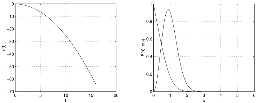
and it can be seen in Figure 4. Plots are also shown of $E(s)$ and $\sigma(t)$.

Figure 4: Painlevé V (left), $E(s)$ and $p(s)$ (right).

2.3 The Prolate Matrix

Another method to calculate the distribution of the eigenvalue spacings is to compute the eigenvalues $\lambda_{i}$ of the operator

$$f(y)\rightarrow\int_{-1}^{1}Q(x,y)f(y)\,dy,\qquad Q(x,y)=\frac{\sin\left((x-y)\pi t\right)}{(x-y)\pi}.$$ (34)

Then $E(2t)=\prod_{i}(1-\lambda_{i})$, and $p(s)$ can be computed as before. To do this, first define the infinite symmetric Prolate matrix:

$$A_{\infty}=\begin{pmatrix}a_{0}&a_{1}&\ldots\\ a_{1}&a_{0}&\ldots\\ \vdots&\vdots&\ddots\end{pmatrix}$$ (35)

with $a_{0}=2w$, $a_{k}=(\sin 2\pi wk)/\pi k$ for $k=1,2,\ldots$, and $0<w<\frac{1}{2}$. A discretization of $Q(x,y)$ is achieved by setting $w=t/n$ and extracting the upper-left $n\times n$ submatrix $A_{n}$ of $A_{\infty}$.

Below, the full matrix $A_{n}$ is used, and all the eigenvalues are computed in $n^{3}$ time using the eig function. However, $A_{n}$ commutes with the following symmetric tridiagonal matrix [4], and therefore has the same eigenvectors:

$$T_{n}=\begin{pmatrix}\alpha_{1}&\beta_{1}&&&\\ \beta_{1}&\alpha_{2}&\beta_{2}&&\\ &\ddots&\ddots&\ddots&\\ &&\beta_{n-2}&\alpha_{n-1}&\beta_{n-1}\\ &&&\beta_{n-1}&\alpha_{n}\end{pmatrix}$$ (36)

where

$$\left\{\begin{array}[]{rcl}\alpha_{k}&=&\left(\frac{n+1}{2}-k\right)^{2}\cos 2\pi w\\ \beta_{k}&=&\frac{1}{2}k(n-k).\end{array}\right.$$ (39)

It is then in principle possible to use the new techniques described in [1] to compute all the eigenvalues and eigenvectors of $T_{n}$ in $n^{2}$ time, and then get the eigenvalues of $A_{n}$ by dot products. This is not done in this example.

The code for computing $E(s)$ is shown below. This time, $p(s)$ is evaluated by numerical differentiation since no information about the derivative of $E(s)$ is available.

  s=0:0.01:5;
  n=100;
  E0=zeros(size(s));
  for ii=1:length(s)
    Q=gallery(’prolate’,n,s(ii)/2/n);
    E0(ii)=prod(1-eig(Q));
  end
  p0=gradient(gradient(E0,s),s);

To improve the accuracy in $E(s)$, Richardson extrapolation can be used. This is done as follows, where the values are assumed to converge as $1/n^{2}$:

  % ... Compute s and E using Painleve V in previous section

  Es=zeros(length(t),0);
  E1=zeros(size(s));
  for n=20*2.^(0:3)
    for ii=1:length(s)
      Q=gallery(’prolate’,n,s(ii)/2/n);
      E1(ii)=prod(1-eig(Q));
    end
    Es=[Es,E1];
  end

  for ii=1:3
    max(abs(Es-E(:,ones(1,size(Es,2)))))
    Es=Es(:,2:end)+diff(Es,1,2)/(2^(ii+1)-1);
  end
  max(abs(Es-E))

The errors $\max_{0\leq s\leq 5}\left|E_{1}(s)-E(s)\right|$ are shown in Table 1, for $n=20,40,80$, and $160$. The error after all extrapolations is of the same order as the “exact solution” using Painlevé V.

N	Error 0	Error 1	Error 2	Error 3
20	0.2244
40	0.0561	0.7701
80	0.0140	0.0483	0.5486
160	0.0035	0.0032	0.0323	2.2673
	$\cdot 10^{-3}$	$\cdot 10^{-7}$	$\cdot 10^{-8}$	$\cdot 10^{-11}$

Table 1: Difference between Prolate solution $E_{1}(s)$ and Painlevé V solution $E(s)$ after 0, 1, 2, and 3 Richardson extrapolations.

2.4 Riemann Zeta Zeros

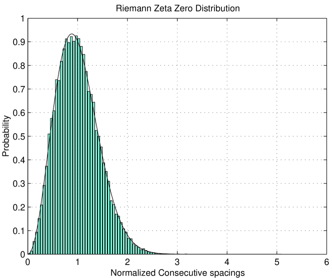
It has been observed that the zeros of the Riemann zeta function along the critical line $\mathrm{Re}(z)=\frac{1}{2}$ behave similar to the eigenvalues of random matrices in the GUE. Here, the distribution of the scaled spacings of the zeros is compared to the corresponding distribution for eigenvalues computed using the Painlevé V equation from the previous chapters.

Define the $n$th zero $\gamma_{n}=n^{\mathrm{th}}$ as

$$\zeta\left(\frac{1}{2}+i\gamma_{n}\right)=0,\qquad 0<\gamma_{1}<\gamma_{2}<\ldots$$ (40)

Compute a normalized spacing:

$$\tilde{\gamma}_{n}=\frac{\gamma_{n}}{\textrm{av spacing near $\gamma_{n}$}}=\gamma_{n}\cdot\left[\frac{\log\gamma_{n}/2\pi}{2\pi}\right].$$ (41)

Zeros of the Riemann zeta function can be downloaded from [3]. Assuming that the MATLAB variable gamma contains the zeros, and the variable offset the offset, these two lines compute the consecutive spacings $\tilde{\gamma}_{n+1}-\tilde{\gamma}_{n}$ and plot the histogram:

  delta=diff(gamma)/2/pi.*log((gamma(1:end-1)+offset)/2/pi);
  histdistr(delta,0:0.05:5.0);

The result can be found in Figure 5, along with the Painlevé V distribution. The curves are indeed in good agreement, although the number of samples here is a little to low to get a perfect match.

Figure 5: Probability distribution of consecutive spacings of Riemann zeta zeros ($30,000$ zeros, $n\approx 10^{12},10^{21},10^{22}$)

References

- [1] Inderjit S. Dhillon. A new algorithm for the symmetric tridiagonal eigenvalue/eigenvector problem. PhD thesis, University of California, Berkeley, 1997.
- [2] Ioana Dumitriu and Alan Edelman. Matrix models for beta ensembles. J. Math. Phys., 43(11):5830–5847, 2002.
- [3] Andrew Odlyzko. Tables of zeros of the riemann zeta function. http://www.dtc.umn.edu/odlyzko/zeta_tables/index.html.
- [4] David Slepian. Prolate spheroidal wave functions, Fourier analysis and uncertainity. IV. Extensions to many dimensions; generalized prolate spheroidal functions. Bell System Tech. J., 43:3009–3057, 1964.
- [5] Craig A. Tracy and Harold Widom. Introduction to random matrices. In Geometric and quantum aspects of integrable systems (Scheveningen, 1992), volume 424 of Lecture Notes in Phys., pages 103–130. Springer, Berlin, 1993.
- [6] Craig A. Tracy and Harold Widom. The distribution of the largest eigenvalue in the Gaussian ensembles: . In Calogero-Moser-Sutherland models (Montréal, QC, 1997), CRM Ser. Math. Phys., pages 461–472. Springer, New York, 2000.
- [7] Lloyd N. Trefethen and David Bau, III. Numerical linear algebra. Society for Industrial and Applied Mathematics (SIAM), Philadelphia, PA, 1997.