LANGEVIN TRAJECTORIES BETWEEN FIXED CONCENTRATIONS

Abstract

We consider the trajectories of particles diffusing between two infinite baths of fixed concentrations connected by a channel, e.g. a protein channel of a biological membrane. The steady state influx and efflux of Langevin trajectories at the boundaries of a finite volume containing the channel and parts of the two baths is replicated by termination of outgoing trajectories and injection according to a residual phase space density. We present a simulation scheme that maintains averaged fixed concentrations without creating spurious boundary layers, consistent with the assumed physics.

I Introduction

We consider particles that diffuse in a domain $\Omega$ connecting two regions, where fixed, but possibly different concentrations are maintained by connection to practically infinite reservoirs. This is the situation in the diffusion of ions through a protein channel of a biological membrane that separates two salt solutions of different fixed concentrations Hille .

Continuum theories of such diffusive systems describe the concentration field by the Nernst-Planck equation (NPE) with fixed boundary concentrations Hille -SNE1 . On the other hand, the underlying microscopic theory of diffusion describes the motion of the diffusing particles by Langevin’s equations BRR , SNE1 -book . This means that on a microscopic scale there are fluctuations in the concentrations at the boundaries. The question of the boundary behavior of the Langevin trajectories (LT), corresponding to fixed boundary concentrations, arises both in theory and in the practice of particle simulations of diffusive motion Tildesley -Im .

When the concentrations are maintained by connection to infinite reservoirs, there are no physical sources and absorbers of trajectories at any definite location in the reservoir or in $\Omega$. The boundaries in this setup can be chosen anywhere in the reservoirs, where the average concentrations are effectively fixed. Nothing unusual happens to the LT there. Upon reaching the boundary they simply cross into the reservoir and may cross the boundary back and forth any number of times. Limiting the system to a finite region necessarily puts sources and absorbers at the interfaces with the baths, as described in Unidir .

The boundary behavior of diffusing particles in a finite domain $\Omega$ has been studied in various cases, including absorbing, reflecting, sticky boundaries, and many other modes of boundary behavior Mandl , Karlin . In Schumaker a sequence of Markovian jump processes is constructed such that their transition probability densities converge to the solution of the Nernst-Planck equation with given boundary conditions, including fixed concentrations and sticky boundaries. Brownian dynamics simulations with different boundary protocols seem to indicate that density fluctuations near the channels are independent of the boundary conditions, if the boundaries are moved sufficiently far away from the channel Corry2002 . However, as shown in PRE , many boundary protocols for maintaining fixed concentrations lead to the formation of spurious boundary layers, which in the case of charged particles may produce large long range fluctuations in the electric field that spread throughout the entire simulation volume $\Omega$. The analytic structure of these boundary layers was determined in Marshall ; Hagan , following several numerical investigations (e.g, Titulaer81 ).

It seems that the boundary behavior of LT of particles diffusing between fixed concentrations has not been described mathematically in an adequate way. From the theoretical point of view, the absence of a rigorous mathematical theory of the boundary behavior of LT diffusing between fixed concentrations, based on the physical theory of the Brownian motion, is a serious lacuna in classical physics.

It is the purpose of this letter to analyze the boundary behavior of LT between fixed concentrations and to design a Langevin simulation that does not form spurious boundary layers. We find the joint probability density function of the velocities and locations, where new simulated LT are injected into a given simulation volume, while maintaining the fixed concentrations. As the time step decreases the simulated density converges to the solution of the Fokker-Planck equation (FPE) with the imposed boundary conditions without forming boundary layers.

II Trajectories, fluxes, and boundary concentrations

We assume fixed concentrations $C_{L}$ and $C_{R}$ on the left and right interfaces between $\Omega$ and the baths $B$, respectively, with all other boundaries of $\Omega$ being impermeable walls, where the normal particle flux vanishes. We assume that the particles interact only with a mean field, whose potential is $\Phi(\mbox{\boldmath$x$})$, so the diffusive motion of a particle in the channel and in the reservoirs is described by the Langevin equation (LE)

$$\ddot{\mbox{\boldmath$x$}}+\gamma(\mbox{\boldmath$x$})\dot{\mbox{\boldmath$x$}}+\nabla_{\mbox{\boldmath$x$}}\Phi(\mbox{\boldmath$x$}) = \sqrt{2\gamma(\mbox{\boldmath$x$})\varepsilon}\,\dot{\mbox{\boldmath$w$}}$$

$$\mbox{\boldmath$x$}(0)=\mbox{\boldmath$x$}_{0},\quad\mbox{\boldmath$v$}(0) = \mbox{\boldmath$v$}_{0},$$

where $\gamma(\mbox{\boldmath$x$})$ is the (state-dependent) friction per unit mass, $\varepsilon$ is a thermal factor, and $\dot{\mbox{\boldmath$w$}}$ is a vector of standard independent Gaussian $\delta$-correlated white noises book .

The probability density function (pdf) of finding the trajectory of the diffusing particle at location $x$ with velocity $v$ at time $t$, given its initial position, satisfies the Fokker-Planck equation (FPE) in the bath and in the reservoirs,

$$\frac{\partial p}{\partial t} = -\mbox{\boldmath$v$}\cdot\nabla_{\mbox{\boldmath$x$}}\,p+\gamma(\mbox{\boldmath$x$})\varepsilon\Delta_{\mbox{\boldmath$v$}}p$$

$$+\nabla_{\mbox{\boldmath$v$}}\cdot\Big{[}\gamma(\mbox{\boldmath$x$})\mbox{\boldmath$v$}+\nabla_{\mbox{\boldmath$x$}}\Phi(\mbox{\boldmath$x$})\Big{]}p,$$

$$p(\mbox{\boldmath$x$},\mbox{\boldmath$v$},0\,|\,\mbox{\boldmath$x$}_{0},\mbox{\boldmath$v$}_{0}) = \delta(\mbox{\boldmath$x$}-\mbox{\boldmath$x$}_{0},\mbox{\boldmath$v$}-\mbox{\boldmath$v$}_{0}).$$

In the Smoluchowski limit of large friction the stationary solution of (II) admits the form EKS

$$p(\mbox{\boldmath$x$},{\mbox{\boldmath$v$}})=\frac{e^{-|\mbox{\boldmath$v$}|^{2}/2\varepsilon}}{(2\pi\varepsilon)^{3/2}}\left\{p(\mbox{\boldmath$x$})+\frac{{\cal J}(\mbox{\boldmath$x$})\cdot\mbox{\boldmath$v$}}{\varepsilon}+O\left(\frac{1}{\gamma^{2}}\right)\right\}$$ (3)

where the flux density vector ${\cal J}(\mbox{\boldmath$x$})$ is given by

$${\cal J}(\mbox{\boldmath$x$})=-\frac{1}{\gamma\left(\mbox{\boldmath$x$}\right)}\bigg{\{}\varepsilon\nabla p(\mbox{\boldmath$x$})+p(\mbox{\boldmath$x$})\,\nabla\Phi(\mbox{\boldmath$x$})\bigg{\}}+O\left(\frac{1}{\gamma^{2}}\right),$$

and $p(\mbox{\boldmath$x$})$ satisfies

$$-\nabla\cdot{\cal J}(\mbox{\boldmath$x$})=\nabla\cdot\frac{1}{\gamma\left(\mbox{\boldmath$x$}\right)}\bigg{\{}\varepsilon\nabla p(\mbox{\boldmath$x$})+p(\mbox{\boldmath$x$})\,\nabla\Phi\left(\mbox{\boldmath$x$}\right)\bigg{\}}=0.$$

In one dimension, the stationary pdfs of velocities of the particles crossing the interface into the given volume are

$$p_{L}(v) \sim \frac{\displaystyle\frac{e^{-v^{2}/2\varepsilon}}{\sqrt{2\pi\varepsilon}}\left\{1+\displaystyle\frac{{\cal J}v}{\varepsilon C_{L}}\right\}}{\displaystyle\frac{1}{2}+\displaystyle\frac{{\cal J}}{C_{L}\sqrt{2\pi\varepsilon}}}\quad\mbox{for}\quad v>0,$$

$$p_{R}(v) \sim \frac{\displaystyle\frac{e^{-v^{2}/2\varepsilon}}{\sqrt{2\pi\varepsilon}}\left\{1-\displaystyle\frac{{\cal J}v}{\varepsilon C_{R}}\right\}}{\displaystyle\frac{1}{2}+\displaystyle\frac{{\cal J}}{C_{R}\sqrt{2\pi\varepsilon}}}\quad\mbox{for}\quad v<0,$$

where ${\cal J}$ is the net probability flux through the channel. The source strengths (unidirectional fluxes at the interfaces) are given by EKS

$$J_{L} = \sqrt{\frac{\varepsilon}{2\pi}}C_{L}-\frac{{\cal J}}{2}+O\left(\frac{1}{\gamma^{2}}\right)$$

$$J_{R} = \sqrt{\frac{\varepsilon}{2\pi}}C_{R}+\frac{{\cal J}}{2}+O\left(\frac{1}{\gamma^{2}}\right).$$

III Application to simulation

Langevin simulations of ion permeation in a protein channel of a biological membrane have to include a part of the surrounding bath, because boundary conditions at the ends of the channel are unknown. The boundary of the simulation has to be interfaced with the bath in a manner that does not distort the physics. This means that new LT have to be injected into the simulation at the correct rate and with the correct distribution of displacement and velocity, for otherwise, spurious boundary layers will form PRE .

Consider a single simulated trajectory that jumps according to the discretized LE (LABEL:LEs)

$$\mbox{\boldmath$x$}(t+\Delta t) = \mbox{\boldmath$v$}(t)\Delta t,\quad\mbox{\boldmath$v$}(t+\Delta t)=\mbox{\boldmath$v$}(t)(1-\gamma\Delta t)$$ (6)

$$- \nabla_{\mbox{\boldmath$x$}}\Phi(\mbox{\boldmath$x$}(t))\Delta t+\sqrt{2\varepsilon\gamma}\,\Delta\mbox{\boldmath$w$}(t),$$

where $\Delta w$ is normally distributed with zero mean and variance $\Delta t$. The trajectory is terminated when it exits $\Omega$ for the first time. The problem at hand is to determine an injection scheme of new trajectories into $\Omega$ such that the interface concentrations are maintained on the average at their nominal values $C_{L}$ and $C_{R}$ and the simulated density profile satisfies (3).

To be consistent with (3), the injection rate has to be equal to the unidirectional flux at the boundary (LABEL:unismolRL). New trajectories have to be injected with displacement and velocity as though the simulation extends outside $\Omega$, consistently with the scheme (6), because the interface is a fictitious boundary. The scheme (6) can move the trajectory from the bath $B$ into $\Omega$ from any point $\mbox{\boldmath$\xi$}\in B$ and with any velocity $\eta$. The probability that a trajectory, which is moved with time step $\Delta t$ from the bath into $\Omega$, or from $\Omega$ into the bath will land exactly on the boundary is zero. It follows that the pdf of the point $(\mbox{\boldmath$x$},\mbox{\boldmath$v$})$, where the trajectory lands in $\Omega$ in one time step, at time $t^{\prime}=t+\Delta t$, say, given that it started at a bath point $(\mbox{\boldmath$\xi$},\mbox{\boldmath$\eta$})$ (in phase space) is, according to (6),

$$\Pr\{\mbox{\boldmath$x$}(t^{\prime})=\mbox{\boldmath$x$},\mbox{\boldmath$v$}(t^{\prime})=\mbox{\boldmath$v$}\,|\,\mbox{\boldmath$x$}(t)=\mbox{\boldmath$\xi$},\mbox{\boldmath$v$}(t)=\mbox{\boldmath$\eta$}\}$$

$$=\frac{\delta(\mbox{\boldmath$x$}-\mbox{\boldmath$\xi$}-\mbox{\boldmath$\eta$}\Delta t)}{(4\pi\varepsilon\gamma\Delta t)^{3/2}}\times$$ (7)

$$\exp\left\{-\displaystyle\frac{\left|\mbox{\boldmath$v$}-\mbox{\boldmath$\eta$}-(\gamma\mbox{\boldmath$v$}+\nabla\Phi(\mbox{\boldmath$\xi$}))\Delta t\right|^{2}}{4\varepsilon\gamma\Delta t}\right\}+o(\Delta t).$$

The stationary pdf $p(\mbox{\boldmath$\xi$},\mbox{\boldmath$\eta$})$ of such a bath point is given in (3). The conditional probability of such a landing is

$$\Pr\{\mbox{\boldmath$x$},\mbox{\boldmath$v$}\,|\,\mbox{\boldmath$x$}\in\Omega,\mbox{\boldmath$\xi$}\in B\}=$$ (8)

$$\frac{\displaystyle\int_{\hbox{\bb R}^{3}}d\mbox{\boldmath$\eta$}\displaystyle\int_{B}d\mbox{\boldmath$\xi$}\Pr\{\mbox{\boldmath$v$}(t^{\prime})=\mbox{\boldmath$v$},\mbox{\boldmath$x$}(t^{\prime})=\mbox{\boldmath$x$}\,|\,\mbox{\boldmath$\xi$},\mbox{\boldmath$\eta$}\}p(\mbox{\boldmath$\xi$},\mbox{\boldmath$\eta$})}{\Pr\{\mbox{\boldmath$x$}\in\Omega,\mbox{\boldmath$\xi$}\in B\}},$$

where the denominator is a normalization constant such that

$$\int_{\hbox{\bb R}^{3}}d\mbox{\boldmath$v$}\int_{\Omega}d\mbox{\boldmath$x$}\,\Pr\{\mbox{\boldmath$x$},\mbox{\boldmath$v$}\,|\,\mbox{\boldmath$x$}\in\Omega,\mbox{\boldmath$\xi$}\in\mbox{B}\}=1.$$

Thus the first point of a new trajectory is chosen according to the pdf (8) and the subsequent points are generated according (6), that is, with the transition pdf (7), until the trajectory leaves $\Omega$. By construction, this scheme recovers the joint pdf (3) in $\Omega$, so no spurious boundary layer is formed.

As an example, we consider a one-dimensional Langevin dynamics simulation of diffusion of free particles between fixed concentrations on a given interval. Assuming that in a channel of length $L$

$$\frac{(C_{L}-C_{R})\sqrt{\varepsilon}}{\gamma L}\ll C_{L},$$

which means that $\gamma$ is sufficiently large, the flux term in eq.(3) is negligible relative to the concentration term. The concentration term is linear with slope ${\cal J}$ and thus can be approximated by a constant, so that $p(\xi)=p(0)+O\left(\gamma^{-1}\right)$ in the left bath. Actually, the value of $p(0)\neq 0$ is unimportant, because it cancels out in the normalized pdf (8), which comes out to be

$$\Pr\{x,v\,|\,x>0,\xi<0\}=\frac{\exp\left\{-\displaystyle\frac{v^{2}}{2\epsilon[1+(\gamma\Delta t)^{2}]}\right\}}{2\epsilon\Delta t\sqrt{1+(\gamma\Delta t)^{2}}}$$

(9)

$$\times\mbox{erfc}\left(\sqrt{\displaystyle\frac{1+(\gamma\Delta t)^{2}}{4\epsilon\gamma\Delta t}}\left(\frac{x}{\Delta t}-v\frac{1-\gamma\Delta t}{1+(\gamma\Delta t)^{2}}\right)\right).$$

In the limit $\Delta t\to 0$ we obtain from eq.(9)

$$\Pr\{x,v\,|\,x>0,\xi<0\}\to\frac{2\delta(x)H(v)}{\sqrt{2\pi\varepsilon}}e^{-v^{2}/2\varepsilon},$$ (10)

where $H(v)$ is the Heaviside unit step function. This means that with the said approximation, LT enter at $x=0$ with a Maxwellian distribution of positive velocities. Without the approximation the limiting distribution of velocities is (LABEL:pvR). Note, however, that injecting trajectories by any Markovian scheme, with the limiting distribution (10) and with any time step $\Delta t$, creates a boundary layer PRE .

A LD simulation with $C_{L}\neq 0,\ C_{R}=0$, and the parameters $\gamma=100,\ \varepsilon=1,\ L=1,\ \Delta t=10^{-4}$ with 25000 trajectories, once with a Maxwellian distribution of velocities at the boundary $x=0$ (red) and once with the pdf (9) (blue) shows that a boundary layer is formed in the former, but not in the latter (see Figure 1).

An alternative way to interpret eq.(9) is to view the simulation (6) as a discrete time Markovian process $(\mbox{\boldmath$x$}(t),\mbox{\boldmath$v$}(t))$ that never enters or exits $\Omega$ exactly at the boundary. If, however, we run a simulation in which particles are inserted at the boundary, the time of insertion has to be random, rather than a lattice time $n\Delta t$. Thus the time of the first jump from the boundary into the domain is the residual time $\Delta t^{\prime}$ between the moment of insertion and the next lattice time $(n+1)\Delta t$. The probability density of jump size in both variables has to be randomized with $\Delta t^{\prime}$, with the result (9).

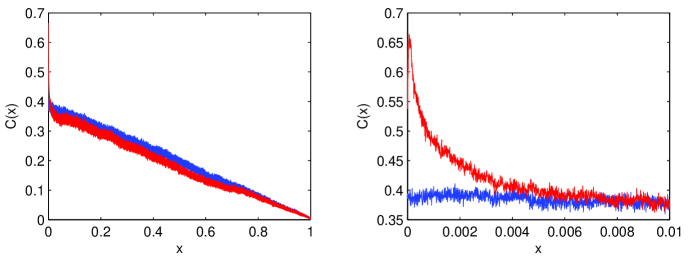
Figure 1: Left panel: Concentration against displacement of a LD simulation with injecting particles according to the residual distribution (9) (blue), and according to the Maxwellian velocity distribution (10) exactly at the boundary (red). The two graphs are almost identical, except for a small boundary layer near $x=0$ in red. Right panel: Zoom in of the concentration profile in the boundary layer $x<0.01=\sqrt{\epsilon}/\gamma$.

.

- (1) Hille, B., 2001, Ionic Channels of Excitable Membranes , Sinauer Associates Inc. Sunderland, pp.1-814. 3rd ed.
- (2) R.S. Berry, S. Rice, J. Ross, Physical Chemistry, second edition, Oxford University Press, 2000.
- (3) W. Nonner, R.S. Eisenberg, Biophys. J. 75, pp. 1287-1305 (1998).
- (4) Z. Schuss, B. Nadler, R.S. Eisenberg, Phys. Rev. E, 64 (2-3) 036116, September (2001).
- (5) R.S. Eisenberg, M.M. Kłosek, Z. Schuss, J. Chem. Phys. 102, pp.1767-1780 (1995).
- (6) Z. Schuss, Theory and Applications of Stochastic Differential Equations, Wiley, NY 1980.
- (7) M.P. Allen, D.J. Tildesley. Computer Simulation of Liquids, Oxford University Press, Oxford 1991.
- (8) B. Corry, S. Kuyucak, S. Chung, Biophys. J. 78, pp.2364-2381 (2000).
- (9) M. Berkowitz and J.A. McCammon, Chem. Phys. Lett. 90, pp.215-217 (1982).
- (10) C.L Brooks, III, and M. Karplus, J. Chem. Phys. 79, p.6312 (1983).
- (11) T. Naeh, Simulation of Ionic Solution, Ph.D. dissertation. Department of Mathematics, Tel-Aviv University 2001.
- (12) B. Nadler, T. Naeh, Z. Schuss, SIAM J. Appl. Math. 62 (2), pp.433-447, (2001).
- (13) B. Nadler, T. Naeh, Z. Schuss, SIAM J. Appl. Math. 63 (3), pp.850-873 (2003).
- (14) W. Im, S. Seefeld, B. Roux, Biophys. J., 79:788-801, (2000).
- (15) A. Singer and Z. Schuss, “Brownian simulations and uni-directional flux in diffusion”, Phys. Rev. E (in press).
- (16) P. Mandl, Analytical Treatment of One-dimensional Markov Processes, Springer Verlag, NY 1968.
- (17) S. Karlin and H.M. Taylor, A First Course in Stochastic Processes, Academic Press, NY 1975.
- (18) M. Schumaker, Journal of Chemical Physics 117 (6), pp.2469-2473 (2002).
- (19) B. Corry, M. Hoyles, T.W. Allen, M. walker, S. Kuyucak, S.H. Chung, Biophys. J. 82, pp.1975-1984, (2002).
- (20) A. Singer, Z. Schuss, B. Nadler, R. S. Eisenberg, “Memoryless control of boundary concentrations of diffusing particles”, Phys. Rev. E. (in press).
- (21) T. W. Marshall, E. J. Watson, J. Phys. A, 18, pp. 3531-3559, (1985).
- (22) P. S. Hagan, C. R. Doering, C. D. Levermore, Siam J. Appl. Math., 49, No. 5, pp. 1480-1513, (1989).
- (23) M. A. Burschka, U. M. Titulaer, J. Stat. Phys., 25, pp. 569-582, (1981).