BROWNIAN SIMULATIONS AND UNI-DIRECTIONAL FLUX IN DIFFUSION

I Introduction

The prediction of ionic currents in protein channels of biological membranes is one of the central problems of computational molecular biophysics. None of the existing continuum descriptions of ionic permeation captures the rich phenomenology of the patch clamp experiments Hille . It is therefore necessary to resort to particle simulations of the permeation process Im1 -Trudy1 . Computer simulations are necessarily limited to a relatively small number of mobile ions, due to computational difficulties. Thus a reasonable simulation can describe only a small portion of the experimental setup of a patch clamp experiment, the channel and its immediate surroundings. The inclusion in the simulation of a part of the bath and its connection to the surrounding bath are necessary, because the conditions at the boundaries of the channel are unknown, while they are measurable in the bath, away from the channel.

Thus the trajectories of the particles are described individually for each particle inside the simulation volume, while outside the simulation volume they can be described only by their statistical properties. It follows that on one side of the interface between the simulation and the surrounding bath the description of the particles is discrete, while a continuum description has to be used on the other side. This poses the fundamental question of how to describe the particle trajectories at the interface, which is the subject of this paper.

We address this problem for Brownian dynamics (BD) simulations, connected to a practically infinite surrounding bath by an interface that serves as both a source of particles that enter the simulation and an absorbing boundary for particles that leave the simulation. The interface is expected to reproduce the physical conditions that actually exist on the boundary of the simulated volume. These physical conditions are not merely the average electrostatic potential and local concentrations at the boundary of the volume, but also their fluctuation in time. It is important to recover the correct fluctuation, because the stochastic dynamics of ions in solution are nonlinear, due to the coupling between the electrostatic field and the motion of the mobile charges, so that averaged boundary conditions do not reproduce correctly averaged nonlinear response. In a system of noninteracting particles incorrect fluctuation on the boundary may still produce the correct response outside a boundary layer in the simulation region Spain .

The boundary fluctuation consists of arrival of new particles from the bath into the simulation and of the recirculation of particles in and out of the simulation. The random motion of the mobile charges brings about the fluctuation in both the concentrations and the electrostatic field. Since the simulation is confined to the volume inside the interface, the new and the recirculated particles have to be fed into the simulation by a source that imitates the influx across the interface. The interface does not represent any physical device that feeds trajectories back into the simulation, but is rather an imaginary wall, which the physical trajectories of the diffusing particles cross and recross any number of times. The efflux of simulated trajectories through the interface is seen in the simulation, however, the influx of new trajectories, which is the unidirectional flux (UF) of diffusion, has to be calculated so as to reproduce the physical conditions, as mentioned above. Thus the UF is the source strength of the influx, and also the number of trajectories that cross the interface in one direction per unit time.

The mathematical problem of the UF begins with the description of diffusion by the diffusion equation. The diffusion equation (DE) is often considered to be an approximation of the Fokker-Planck equation (FPE) in the Smoluchowski limit of large damping. Both equations can be written as the conservation law

$$\frac{\partial p}{\partial t}=-\nabla\cdot\mbox{\boldmath$J$}.$$ (1)

The flux density $J$ in the diffusion equation is given by

$$\mbox{\boldmath$J$}(\mbox{\boldmath$x$},t)=-\frac{1}{\gamma}\left[\varepsilon\nabla p(\mbox{\boldmath$x$},t)-\mbox{\boldmath$f$}(\mbox{\boldmath$x$})p(\mbox{\boldmath$x$},t)\right],$$ (2)

where $\gamma$ is the friction coefficient (or dynamical viscosity), $\varepsilon=\displaystyle\frac{k_{B}T}{m}$, $k_{B}$ is Boltzmann’s constant, $T$ is absolute temperature, and $m$ is the mass of the diffusing particle. The external acceleration field is $\mbox{\boldmath$f$}(\mbox{\boldmath$x$})$ and $p(\mbox{\boldmath$x$},t)$ is the density (or probability density) of the particles book . The flux density in the FPE is given by where the net probability flux density vector has the components

$$J_{\mbox{\boldmath$x$}}(\mbox{\boldmath$x$},\mbox{\boldmath$v$},t) = \mbox{\boldmath$v$}p(\mbox{\boldmath$x$},\mbox{\boldmath$v$},t)$$

$$J_{\mbox{\boldmath$v$}}(\mbox{\boldmath$x$},\mbox{\boldmath$v$},t) = -\left(\gamma\mbox{\boldmath$v$}-\mbox{\boldmath$f$}(\mbox{\boldmath$x$})\right)p(\mbox{\boldmath$x$},\mbox{\boldmath$v$},t)-\varepsilon\gamma\nabla_{\mbox{\boldmath$v$}}p(\mbox{\boldmath$x$},\mbox{\boldmath$v$},t).$$

The density $p(\mbox{\boldmath$x$},t)$ in the diffusion equation (1) with (2) is the probability density of the trajectories of the Smoluchowski stochastic differential equation

$$\dot{\mbox{\boldmath$x$}}=\frac{1}{\gamma}\mbox{\boldmath$f$}(\mbox{\boldmath$x$})+\sqrt{\frac{2\varepsilon}{\gamma}}\,\dot{\mbox{\boldmath$w$}},$$ (4)

where $\mbox{\boldmath$w$}(t)$ is a vector of independent standard Wiener processes (Brownian motions).

The density $p(\mbox{\boldmath$x$},\mbox{\boldmath$v$},t)$ is the probability density of the phase space trajectories of the Langevin equation

$$\ddot{\mbox{\boldmath$x$}}+\gamma\dot{\mbox{\boldmath$x$}}=\mbox{\boldmath$f$}(\mbox{\boldmath$x$})+\sqrt{2\varepsilon\gamma}\dot{\mbox{\boldmath$w$}}.$$ (5)

In practically all conservation laws of the type (1) $J$ is a net flux density vector. It is often necessary to split it into two unidirectional components across a given surface, such that the net flux $J$ is their difference. Such splitting is pretty obvious in the FPE, because the velocity $v$ at each point $x$ tells the two UFs apart. Thus, in one dimension,

$$J_{LR}(x,t) = \int_{0}^{\infty}vp(x,v,t)\,dv,\quad J_{RL}(x,t)=-\int_{-\infty}^{0}vp(x,v,t)\,dv$$

$$J_{\mbox{net}}(x,t) = J_{LR}(x,t)-J_{RL}(x,t)=\int_{-\infty}^{\infty}vp(x,v,t)\,dv.$$

In contrast, the net flux $J(x,t)$ in the DE cannot be split this way, because velocity is not a state variable. Actually, the trajectories of a diffusion process do not have well defined velocities, because they are nowhere differentiable with probability 1 DEK . These trajectories cross and recross every point $x$ infinitely many times in any time interval $[t,t+\Delta t]$, giving rise to infinite UFs. However, the net diffusion flux is finite, as indicated in eq.(2). This phenomenon was discussed in detail in unidirect , where a path integral description of diffusion was used to define the UF. The unidirectional diffusion flux, however, is finite at absorbing boundaries, where the UF equals the net flux. The UFs measured in diffusion across biological membranes by using radioactive tracer Hille are in effect UFs at absorbing boundaries, because the tracer is a separate ionic species BobDuan .

An apparent paradox arises in the Smoluchowski approximation of the FPE by the DE, namely, the UF of the DE is infinite for all $\gamma$, while the UF of the FPE remains finite, even in the limit $\gamma\to\infty$, in which the solution of the DE is an approximation of that of the FPE EKS . The “paradox” is resolved by a new derivation of the FPE for LD from the Wiener path integral. This derivation is different than the derivation of the DE or the Smoluchowski equation from the Wiener integral (see, e.g. Kleinert -Freidlin ) by the method of M. Kac Kac . The new derivation shows that the path integral definition of UF in diffusion, as first introduced in unidirect , is consistent with that of UF in the FPE. However, the definition of flux involves the limit $\Delta t\to 0$, that is, a time scale shorter than $1/\gamma$, on which the solution of the DE is not a valid approximation to that of the FPE.

This discrepancy between the Einstein and the Langevin descriptions of the random motion of diffusing particles was hinted at by both Einstein and Smoluchowski. Einstein Einstein remarked that his diffusion theory is based on the assumption that the diffusing particles are observed intermittently at short time intervals, but not too short, while Smoluchowski Smoluchowski06 showed that the variance of the displacement of Langevin trajectories is quadratic in $t$ for times much shorter than the relaxation time $1/\gamma$, but is linear in $t$ for times much longer that $1/\gamma$, which is the same as in Einstein’s theory of diffusion Chandra .

The infinite unidirectional diffusion flux imposes serious limitations on BD simulations of diffusion in a finite volume embedded in a much larger bath. Such simulations are used, for example, in simulations of ion permeation in protein channels of biological membranes Hille . If parts of the bathing solutions on both sides of the membrane are to be included in the simulation, the UFs of particles into the simulation have to be calculated. Simulations with BD would lead to increasing influxes as the time step is refined.

The method of resolution of the said “paradox” is based on the definition of the UF of the Langevin dynamics (LD) in terms of the Wiener path integral, analogous to its definition for the BD in unidirect . The UF $J_{LR}(x,t)$ is the probability per unit time $\Delta t$ of trajectories that are on the left of $x$ at time $t$ and are on the right of $x$ at time $t+\Delta t$. We show that the UF of BD coincides with that of LD if the time unit $\Delta t$ in the definition of the unidirectional diffusion flux is exactly

$$\Delta t=\frac{2}{\gamma}.$$ (7)

We find the strength of the source that ensures that a given concentration is maintained on the average at the interface in a BD simulation. The strength of the left source $J_{LR}$ is to leading order independent of the efflux and depends on the concentration $C_{L}$, the damping coefficient $\gamma$, the temperature $\varepsilon$, and the time step $\Delta t$, as given in eq.(27). To leading order it is

$$J_{LR}=\sqrt{\frac{\varepsilon}{\pi\gamma\Delta t}}\,C_{L}+O\left(\frac{1}{\gamma}\right).$$ (8)

We also show that the coordinate of a newly injected particle has the probability distribution of the residual of the normal distribution. Our simulation results show that no spurious boundary layers are formed with this scheme, while they are formed if new particles are injected at the boundary. The simulations also show that if the injection rate is fixed, there is depletion of the population as the time step is refined, but there is no depletion if the rate is changed according to eq.(8).

In Section II, we derive the FPE for the LD (5) from the Wiener path integral. In Section III, we define the unidirectional probability flux for LD by the path integral and show that is indeed given by (LABEL:Js). In Section IV, we use the results of EKS to calculate explicitly the UF in the Smoluchowski approximation to the solution of the FPE and to recover the flux (2). In Section V, we use the results of unidirect to evaluate the UF of the BD trajectories (4) in a finite time unit $\Delta t$. In the limit $\Delta t\to 0$ the UF diverges, but if it is chosen as in (7), the UFs of LD and BD coincide. In Section VI we describe the a BD simulation of diffusion between fixed concentrations and give results of simulations. Finally, Section VII is a summary and discussion of the results.

II Derivation of the Fokker-Planck equation from a path integral

The LD (5) of a diffusing particle can be written as the phase space system

$$\dot{x}=v,\quad\dot{v}=-\gamma v+f(x)+\sqrt{2\varepsilon\gamma}\,\dot{w}.$$ (9)

This means that in time $\Delta t$ the dynamics progresses according to

$$x(t+\Delta t) = x(t)+v(t)\Delta t+o(\Delta t)$$ (10)

$$v(t+\Delta t) = v(t)+[-\gamma v(t)+f(x(t))]\Delta t+\sqrt{2\varepsilon\gamma}\,\Delta w+o(\Delta t),$$ (11)

where $\Delta w\sim{\cal N}(0,\Delta t)$, that is, $\Delta w$ is normally distributed with mean 0 and variance $\Delta t$. This means that the probability density function evolves according to the propagator

$$\mbox{Prob}\{x(t+\Delta t)=x,v(t+\Delta t)=v\}=p(x,v,t+\Delta t)=o(\Delta t)+$$ (12)

$$\frac{1}{\sqrt{4\varepsilon\gamma\pi\Delta t}}\int_{a}^{b}\!\int_{-\infty}^{\infty}p(\xi,\eta,t)\delta(x-\xi-\eta\Delta t)\exp\left\{-\frac{\left[v-\eta-[-\gamma\eta+f(\xi)]\Delta t\right]^{2}}{4\varepsilon\gamma\Delta t}\right\}\,d\xi\,d\eta.$$

To understand (12), we note that given that the displacement and velocity of the trajectory at time $t$ are $x(t)=\xi$ and $v(t)=\eta$, respectively, then according to eq.(10), the displacement of the particle at time $t+\Delta t$ is deterministic, independent of the value of $\Delta w$, and is $x=\xi+\eta\Delta t+o(\Delta t)$. Thus the probability density function (pdf) of the displacement is $\delta(x-\xi-\eta\Delta t+o(\Delta t))$. It follows that the displacement contributes to the joint propagator (12) of $x(t)$ and $v(t)$ a multiplicative factor of the Dirac $\delta$ function. Similarly, eq.(11) means that the conditional pdf of the velocity at time $t+\Delta t$, given $x(t)=\xi$ and $v(t)=\eta$, is normal with mean $\eta+[-\gamma\eta+f(\xi)]\Delta t+o(\Delta t)$ and variance $2\epsilon\gamma\Delta t+o(\Delta t)$, as reflected in the exponential factor of the propagator. If trajectories are terminated at the ends of an finite or infinite interval $(a,b)$, the integration over the displacement variable extends only to that interval.

The basis for our analysis of the UF is the following new derivation of the Fokker-Planck equation from eq.(12). Integration with respect to $\xi$ gives

$$p(x,v,t+\Delta t)=o(\Delta t)+$$ (13)

$$\frac{1}{\sqrt{4\varepsilon\gamma\pi\Delta t}}\int_{-\infty}^{\infty}p(x-\eta\Delta t,\eta,t)\exp\left\{-\frac{\left[v-\eta-[-\gamma\eta+f(x-\eta\Delta t)]\Delta t\right]^{2}}{4\varepsilon\gamma\Delta t}\right\}\,d\eta.$$

Changing variables to

$$-u=\frac{v-\eta-[-\gamma\eta+f(x-\eta\Delta t)]\Delta t}{{\sqrt{2\varepsilon\gamma\Delta t}}},$$

and expanding in powers of $\Delta t$, the integral takes the form

$$p(x,v,t+\Delta t)=\frac{1}{\sqrt{2\pi}(1-\gamma\Delta t+o(\Delta t))}\int_{-\infty}^{\infty}\,e^{-u^{2}/2}\,du\times$$ (14)

$$p(x-v(1+\gamma\Delta t)\Delta t+o(\Delta t),v(1+\gamma\Delta t)+u\sqrt{2\varepsilon\gamma\Delta t}-f(x)\Delta t(1+\gamma\Delta t)+o(\Delta t),t)$$

Reexpanding in powers of $\Delta t$, we get

$$p(x-v(1+\gamma\Delta t)\Delta t+o(\Delta t),v(1+\gamma\Delta t)+u\sqrt{2\varepsilon\gamma\Delta t}-f(x)\Delta t(1+\gamma\Delta t)+o(\Delta t),t)=$$

$$p(x,v,t)-v\Delta t\frac{\partial p(x,v,t)}{\partial x}+\frac{\partial p(x,v,t)}{\partial v}\left(v\gamma\Delta t+u\sqrt{2\varepsilon\gamma\Delta t}-f(x)\Delta t+o(\Delta t)\right)+$$

$$\varepsilon\gamma u^{2}\Delta t\frac{\partial^{2}p(x,v,t)}{\partial v^{2}}+o(\Delta t),$$

so (14) gives

$$p(x,v,t+\Delta t)-\frac{p(x,v,t)}{1-\gamma\Delta t} = -\frac{1}{1-\gamma\Delta t}v\Delta t\frac{\partial p(x,v,t)}{\partial x}+\frac{\Delta t}{1-\gamma\Delta t}\frac{\partial p(x,v,t)}{\partial v}\left(v\gamma-f(x)\right)$$

$$+ \frac{\varepsilon\gamma\Delta t}{1-\gamma\Delta t}\frac{\partial^{2}p(x,v,t)}{\partial v^{2}}+O\left(\Delta t^{3/2}\right).$$

Dividing by $\Delta t$ and taking the limit $\Delta t\to 0$, we obtain the Fokker-Planck equation in the form

$$\frac{\partial p(x,v,t)}{\partial t}=-v\frac{\partial p(x,v,t)}{\partial x}+\frac{\partial}{\partial v}\left[\left(\gamma v-f(x)\right)p(x,v,t)\right]+\varepsilon\gamma\frac{\partial^{2}p(x,v,t)}{\partial v^{2}},$$ (15)

which is the conservation law (1) with the flux components (LABEL:FPflux). The UF $J_{LR}(x_{1},t)$ is usually defined as the integral of $J_{x}(x_{1},v,t)$ over the positive velocities (EKS, , and references therein), that is,

$$J_{LR}(x_{1},t)=\int_{0}^{\infty}vp(x_{1},v,t)\,dv.$$ (16)

To show that this integral actually represents the probability of the trajectories that move from left to right across $x_{1}$ per unit time, we evaluate below the probability flux from a path integral.

III The unidirectional flux of the Langevin equation

The instantaneous unidirectional probability flux from left to right at a point $x_{1}$ is defined as the probability per unit time ($\Delta t$), of Langevin trajectories that are to the left of $x_{1}$ at time $t$ (with any velocity) and propagate to the right of $x_{1}$ at time $t+\Delta t$ (with any velocity), in the limit $\Delta t\to 0$. This can be expressed in terms of a path integral on Langevin trajectories on the real line as

$$J_{LR}(x_{1},t) = \lim_{\Delta t\to 0}\frac{1}{\Delta t}\int_{-\infty}^{x_{1}}\,d\xi\int_{x_{1}}^{\infty}\,dx\int_{-\infty}^{\infty}\,d\eta\int_{-\infty}^{\infty}\,dv\ \frac{1}{\sqrt{4\varepsilon\gamma\pi\Delta t}}p(\xi,\eta,t)\delta(x-\xi-\eta\Delta t)\times$$ (17)

$$\exp\left\{-\frac{\left[v-\eta-[-\gamma\eta+f(\xi)]\Delta t\right]^{2}}{4\varepsilon\gamma\Delta t}\right\}.$$

Integrating with respect to $v$ eliminates the exponential factor and integration with respect to $\xi$ fixes $\xi$ at $x-\eta\Delta t$, so

$$J_{LR}(x_{1},t) = \lim_{\Delta t\to 0}\frac{1}{\Delta t}\int\!\int_{x-\eta\Delta t<x_{1}}p(x-\eta\Delta t,\eta,t)\,d\eta\,dx$$ (18)

$$= \lim_{\Delta t\to 0}\frac{1}{\Delta t}\int_{0}^{\infty}\,d\eta\int_{x_{1}-\eta\Delta t}^{x_{1}}p(u,\eta,t)\,du$$

$$= \int_{0}^{\infty}\eta p(x_{1},\eta,t)\,d\eta.$$

The expression (18) is identical to (16).

IV The Smoluchowski approximation to the unidirectional current

The following calculations were done in EKS and are shown here for completeness. In the overdamped regime, as $\gamma\to\infty$, the Smoluchowski approximation to $p(x,v,t)$ is given by

$$p(x,v,t)\sim\frac{e^{-v^{2}/2\epsilon}}{\sqrt{2\pi\epsilon}}\left\{p(x,t)-\frac{1}{\gamma}\left[\frac{\partial p(x,t)}{\partial x}-\frac{1}{\epsilon}f(x)p(x,t)\right]v+O\left(\frac{1}{\gamma^{2}}\right)\right\},$$ (19)

where the marginal density $p(x,t)$ satisfies the Fokker-Planck-Smoluchowski equation

$$\gamma\frac{\partial p(x,t)}{\partial t}=\varepsilon\frac{\partial^{2}p(x,t)}{\partial x^{2}}-\frac{\partial}{\partial x}\left[f(x)p(x,t)\right].$$ (20)

According to (16) and (19), the UF is

$$J_{LR}(x_{1},t) = \int_{0}^{\infty}vp(x_{1},v,t)\,dv$$ (21)

$$= \int_{0}^{\infty}v\frac{e^{-v^{2}/2\epsilon}}{\sqrt{2\pi\epsilon}}\left\{p(x,t)-\frac{1}{\gamma}\left[\frac{\partial p(x,t)}{\partial x}-\frac{1}{\epsilon}f(x)p(x,t)\right]v+O\left(\frac{1}{\gamma^{2}}\right)\right\}\,dv$$

$$= \sqrt{\frac{\varepsilon}{2\pi}}p(x_{1},t)-\frac{1}{2\gamma}\left[\varepsilon\frac{\partial p(x,t)}{\partial x}-f(x)p(x,t)\right]+O\left(\frac{1}{\gamma^{2}}\right).$$

Similarly, the UF from right to left is

$$J_{RL}(x_{1},t) = -\int^{0}_{-\infty}vp(x_{1},v,t)\,dv$$ (22)

$$= \sqrt{\frac{\varepsilon}{2\pi}}p(x_{1},t)+\frac{1}{2\gamma}\left[\varepsilon\frac{\partial p(x,t)}{\partial x}-f(x)p(x,t)\right]+O\left(\frac{1}{\gamma^{2}}\right).$$

Both UFs in (21) and (22) are finite and proportional to the marginal density at $x_{1}$. The net flux is the difference

$$J_{\mbox{net}}(x_{1},t)=J_{LR}(x_{1},t)-J_{RL}(x_{1},t)=-\frac{1}{\gamma}\left[\varepsilon\frac{\partial p(x,t)}{\partial x}-f(x)p(x,t)\right],$$ (23)

as in classical diffusion theory EKS , Gardiner .

V The unidirectional current in the Smoluchowski equation

Classical diffusion theory, however, gives a different result. In the overdamped regime the Langevin equation (9) is reduced to the Smoluchowski equation book

$$\gamma\dot{x}=f(x)+\sqrt{2\varepsilon\gamma}\,\dot{w}.$$ (24)

As in Section III, the unidirectional probability current (flux) density at a point $x_{1}$ can be expressed in terms of a path integral as

$$J_{LR}(x_{1},t)=\lim_{\Delta t\rightarrow 0}J_{LR}(x_{1},t,\Delta t),$$ (25)

where

$$J_{LR}(x_{1},t,\Delta t)=\sqrt{\frac{\gamma}{4\pi\varepsilon\Delta t}}\int_{0}^{\infty}d\xi\int_{\xi}^{\infty}d\zeta\,\exp\left\{-\frac{\gamma\zeta^{2}}{4\varepsilon}\right\}\times$$ (26)

$$\left\{p\left(x_{1},t\right)-\sqrt{\Delta t}\left[-\frac{\zeta f(x_{1})}{2\varepsilon}p\left(x_{1},t\right)+\left(\zeta-\xi\right)\frac{\partial p(x_{1},t)}{\partial x}\right]+O\left(\frac{\Delta t}{\gamma}\right)\right\}.$$

It was shown in unidirect that

$$J_{LR}(x_{1},t,\Delta t)=\sqrt{\frac{\varepsilon}{\pi\gamma\Delta t}}\,p(x_{1},t)+\frac{1}{2\gamma}\left(f(x_{1})p(x_{1},t)-\varepsilon\frac{\partial p(x_{1},t)}{\partial x}\right)+O\left(\frac{\sqrt{\Delta t}}{\gamma^{3/2}}\right).$$ (27)

Similarly,

$$J_{RL}(x_{1},t)=\lim_{\Delta t\rightarrow 0}J_{RL}(x_{1},t,\Delta t),$$

where

$$J_{RL}(x_{1},t,\Delta t)=\sqrt{\frac{\gamma}{4\pi\varepsilon\Delta t}}\int_{0}^{\infty}d\xi\int_{\xi}^{\infty}d\zeta\,\exp\left\{-\frac{\gamma\zeta^{2}}{4\varepsilon}\right\}\times$$ (28)

$$\left\{p\left(x_{1},t\right)+\sqrt{\Delta t}\left[-\frac{\zeta f(x_{1})}{2\varepsilon}p\left(x_{1},t\right)+\left(\zeta-\xi\right)\frac{\partial p(x_{1},t)}{\partial x}\right]+O\left(\frac{\Delta t}{\gamma}\right)\right\}.$$

$$= \sqrt{\frac{\varepsilon}{\pi\gamma\Delta t}}\,p(x_{1},t)-\frac{1}{2\gamma}\left(f(x_{1})p(x_{1},t)-\varepsilon\frac{\partial p(x_{1},t)}{\partial x}\right)+O\left(\frac{\sqrt{\Delta t}}{\gamma^{3/2}}\right).$$

If $p(x_{1},t)>0$, then both $J_{LR}(x_{1},t)$ and $J_{RL}(x_{1},t)$ are infinite, in contradiction to the results (21) and (22). However, the net flux density is finite and is given by

$$J_{\mbox{net}}(x_{1},t) = \lim_{\Delta t\rightarrow 0}\left\{J_{LR}(x_{1},t,\Delta t)-J_{RL}(x_{1},t,\Delta t)\right\}$$ (29)

$$= -\frac{1}{\gamma}\left[\varepsilon\frac{\partial}{\partial x}p(x_{1},t)-{f(x_{1})}p(x_{1},t)\right],$$

which is identical to (23).

The apparent paradox is due to the idealized properties of the Brownian motion. More specifically, the trajectories of the Brownian motion, and therefore also the trajectories of the solution of eq.(24), are nowhere differentiable, so that any trajectory of the Brownian motion crosses and recrosses the point $x_{1}$ infinitely many times in any time interval $[t,t+\Delta t]$ ItoMcKean . Obviously, such a vacillation creates infinite UFs.

Not so for the trajectories of the Langevin equation (9). They have finite continuous velocities, so that the number of crossing and recrossing is finite. We note that setting $\gamma\Delta t=2$ in equations (27) and (28) gives (21) and (22).

VI Brownian Simulations

Here we design and analyze a BD simulation of particles diffusing between fixed concentrations. Thus, we consider the free Brownian motion (i.e., $\mbox{\boldmath$f$}=0$ in eq. (4)) in the interval $[0,1]$. The trajectories were produced as follows: a) According to the dynamics (4), new trajectories that are started at $x(-\Delta t)=0$ move to $x(0)=\sqrt{\displaystyle\frac{2\varepsilon}{\gamma}}\left|\Delta w\right|$; b) The dynamics progresses according to the Euler scheme $x(t+\Delta t)=x(t)+\sqrt{\displaystyle\frac{2\varepsilon}{\gamma}}\Delta w$; c) The trajectory is terminated if $x(t)>1$ or $x(t)<0$. The parameters are $\varepsilon=1,\,\gamma=1000,\,\Delta t=1$. We ran 10,000 random trajectories and constructed the concentration profile by dividing the interval into equal parts and recording the time each trajectory spent in each bin prior to termination. The results are shown in Figure 1. The simulated concentration profile is linear, but for a small depletion layer near the left boundary $x=0$, where new particles are injected. This is inconsistent with the steady state DE, which predicts a linear concentration profile in the entire interval $[0,1]$. The discrepancy stems from part (a) of the numerical scheme, which assumes that particles enter the simulation interval exactly at $x=0$. However, $x=0$ is just an imaginary interface. Had the simulation been run on the entire line, particles would hop into the simulation across the imaginary boundary at $x=0$ from the left, rather than exactly at the boundary. This situation is familiar from renewal theory Karlin . The probability distribution of the distance an entering particle covers, not given its previous location, is not normal, but rather it is the residual of the normal distribution, given by

$$f(x)=C\int_{-\infty}^{0}\exp\left\{-\frac{(x-y)^{2}}{2\sigma^{2}}\right\}\,dy,$$ (30)

where $\sigma^{2}=\displaystyle\frac{2\varepsilon\Delta t}{\gamma}$ and $C$ is determined by the normalization condition $\displaystyle\int_{0}^{\infty}f(x)\,dx=1$. This gives

$$f(x)=\sqrt{\frac{\pi}{2\sigma}}\,\mbox{erfc}\left(\frac{x}{\sqrt{2}\sigma}\right).$$ (31)

Rerunning the simulation with the entrance pdf $f(x)$, we obtained the expected linear concentration profile, without any depletion layers (see Figure 2). Injecting particles exactly at the boundary makes their first leap into the simulation too large, thus effectively decreasing the concentration profile near the boundary.

Next, we changed the time step $\Delta t$ of the simulation, keeping the injection rate of new particles constant. The population of trajectories inside the interval was depleted when the time step was refined (see Figure 3). A well behaved numerical simulation is expected to converge as the time step is refined, rather than to result in different profiles. This shortcoming of refining the time step is remedied by replacing the constant rate sources with time-step-dependent sources, as predicted by eqs.(27)-(28). Figure 4 describes the concentration profiles for three different values of $\Delta t$ and source strengths that are proportional to $1/\sqrt{\Delta t}$. The concentration profiles now converge when $\Delta t\to 0$. The key to this remedy is the calculation of the UF in diffusion.

VII Summary and discussion

Both Einstein Einstein and Smoluchowski Smoluchowski06 (see also Chandra ) pointed out that BD is a valid description of diffusion only at times that are not too short. More specifically, the Brownian approximation to the Langevin equation breaks down at times shorter than $1/\gamma$, the relaxation time of the medium in which the particles diffuse.

In a BD simulation of a channel the dynamics in the channel region may be much more complicated than the dynamics near the interface, somewhere inside the continuum bath, sufficiently far from the channel. Thus the net flux is unknown, while the boundary concentration is known. It follow that the simulation should be run with source strengths (27), (28),

$$J_{LR}\sim\sqrt{\frac{\varepsilon}{\pi\gamma\Delta t}}\,C_{L}+\frac{1}{2}J_{\mbox{net}},\quad J_{RL}\sim\sqrt{\frac{\varepsilon}{\pi\gamma\Delta t}}\,C_{R}-\frac{1}{2}J_{\mbox{net}}.$$

However, $J_{\mbox{net}}$ is unknown, so neglecting it relative to $\sqrt{\displaystyle\frac{\varepsilon}{\pi\gamma\Delta t}}\,C_{L,R}$ will lead to steady state boundary concentrations that are close, but not necessarily equal to $C_{L}$ and $C_{R}$. Thus a shooting procedure has to be adopted to adjust the boundary fluxes so that the output concentrations agree with $C_{L}$ and $C_{R}$, and then the net flux can be readily found.

According to (27) and (28), the efflux and influx remain finite at the boundaries, and agree with the fluxes of LD, if the time step in the BD simulation is chosen to be $\Delta t=\displaystyle\frac{2}{\gamma}$ near the boundary. If the time step is chosen differently, the fluxes remain finite, but the simulation does not recover the UF of LD. At points away from the boundary, where correct UFs do not have to be recovered, the simulation can proceed in coarser time steps.

The above analysis can be generalized to higher dimensions. In three dimensions the normal component of the UF vector at a point $x$ on a given smooth surface represents the number of trajectories that cross the surface from one side to the other, per unit area at $x$ in unit time. Particles cross the interface in one direction if their velocity satisfies $\mbox{\boldmath$v$}\cdot\mbox{\boldmath$n$}(\mbox{\boldmath$x$})>0$, where $\mbox{\boldmath$n$}(\mbox{\boldmath$x$})$ is the unit normal vector to the surface at $x$, thus defining the domain of integration for eq.(LABEL:Js).

The time course of injection of particles into a BD simulation can be chosen with any inter-injection probability density, as long as the mean time between injections is chosen so that the source strength is as indicated in (27) and (28). For example, these times can be chosen independently of each other, without creating spurious boundary layers.

A. Singer, PRE, Fig. 1

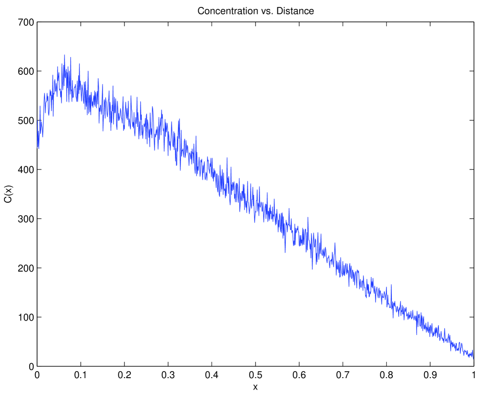
Figure 1: The concentration profile of Brownian trajectories that are initiated at $x=0$ with a normal distribution, and terminated at either $x=0$ or $x=1$.

A. Singer, PRE, Fig. 2

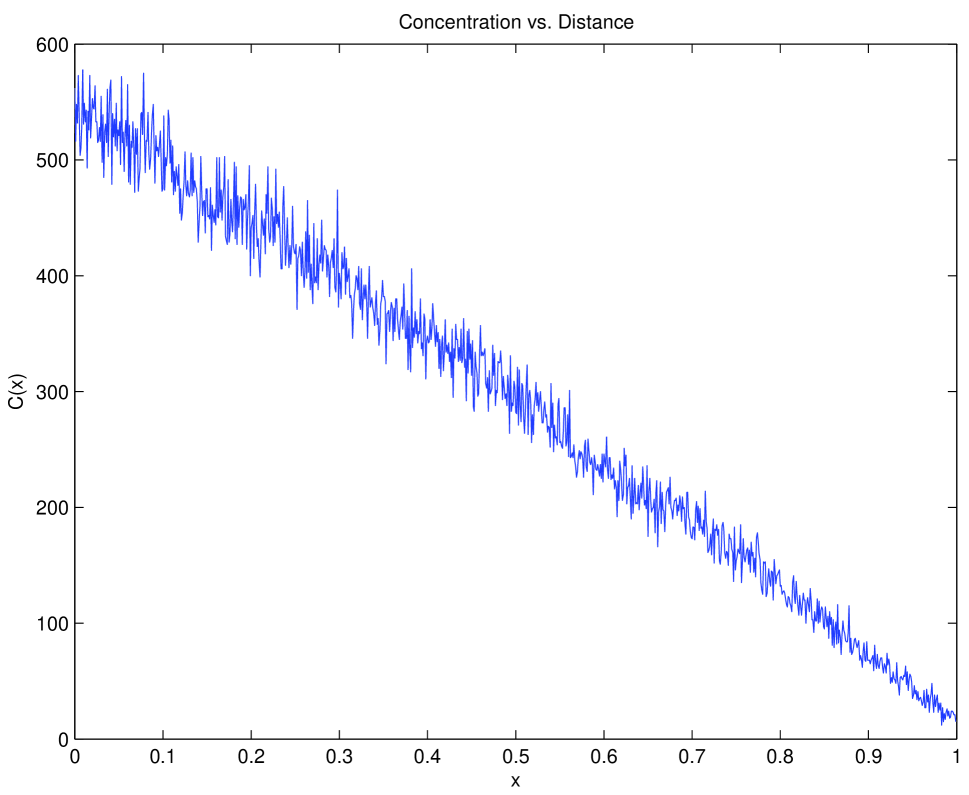
Figure 2: The concentration profile of Brownian trajectories that are initiated at $x=0$ with the residual of the normal distribution, and terminated at either $x=0$ or $x=1$.

A. Singer, PRE, Fig. 3

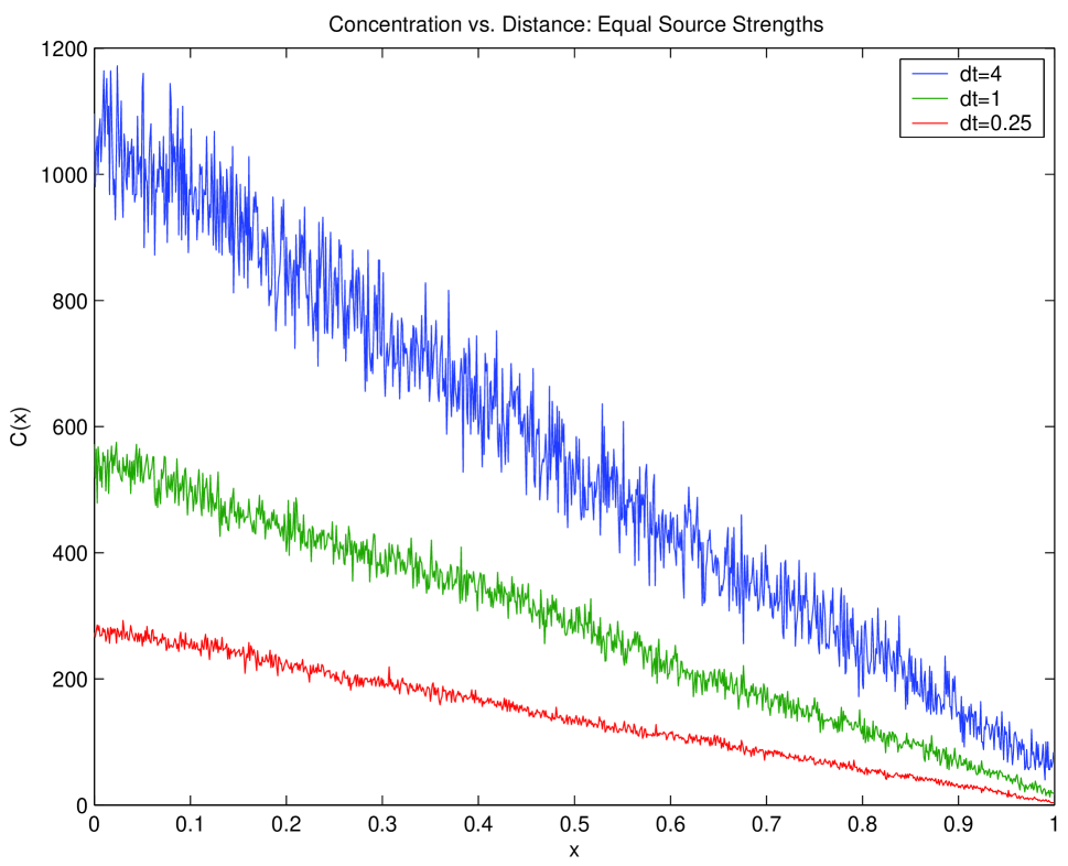
Figure 3: The concentration profile of Brownian trajectories that are initiated at $x=0$ and terminated at either $x=0$ or $x=1$. Three different time steps $(\Delta t=4,1,0.25)$ were used, but the injection rate of new particles remained constant. Refining the time step decreases the concentration profile.

A. Singer, PRE, Fig. 4

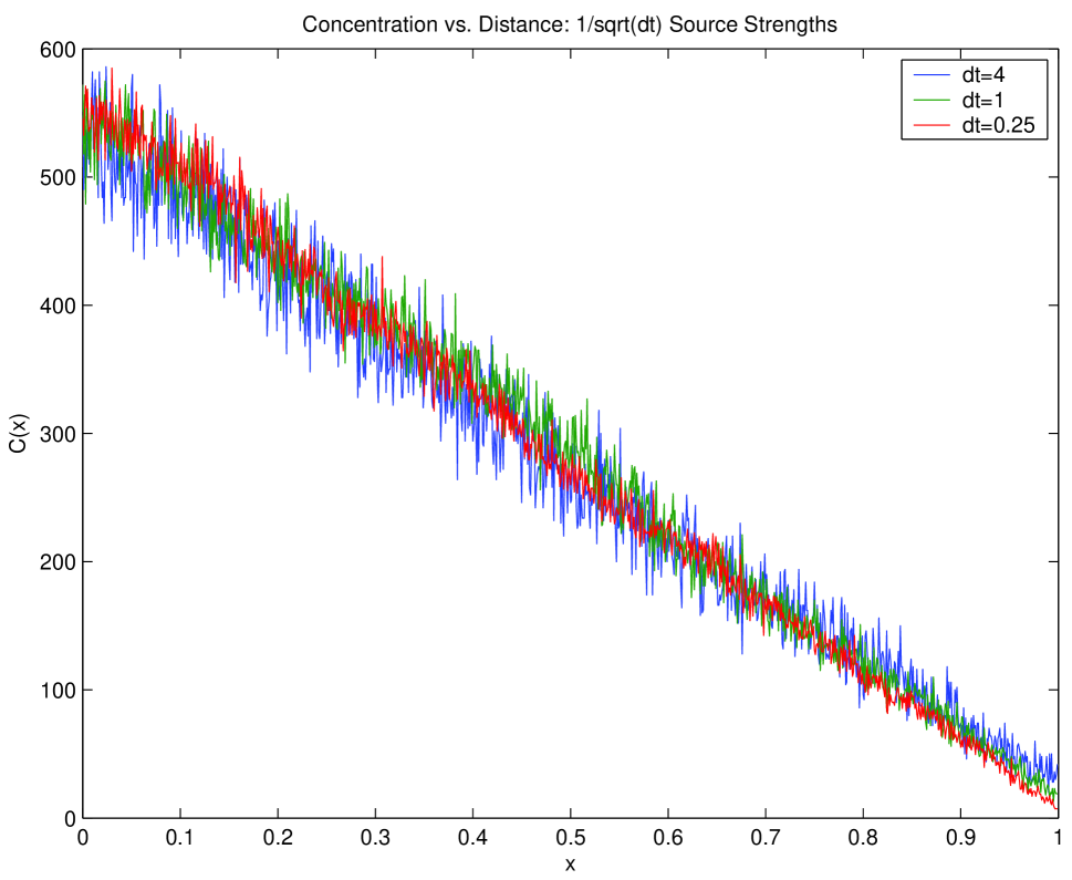
Figure 4: The concentration profile of Brownian trajectories that are initiated at $x=0$ and terminated at either $x=0$ or $x=1$. Three different time steps $(\Delta t=4,1,0.25)$ are shown, and the injection rate of new particles is proportional to $1/\sqrt{\Delta t}$. Refining the time step does not alter the concentration profile.