Abstract

We quantize the 1-dimensional 3-body problem with harmonic and inverse square pair potential by separating the Schrödinger equation following the classic work of Calogero, but allowing all possible self-adjoint boundary conditions for the angular and radial Hamiltonians. The inverse square coupling constant is taken to be $g=2\nu(\nu-1)$ with $\frac{1}{2}<\nu<\frac{3}{2}$ and then the angular Hamiltonian is shown to admit a 2-parameter family of inequivalent quantizations compatible with the dihedral $D_{6}$ symmetry of its potential term $9\nu(\nu-1)/\sin^{2}3\phi$. These are parametrized by a matrix $U\in U(2)$ satisfying $\sigma_{1}U\sigma_{1}=U$, and in all cases we describe the qualitative features of the angular eigenvalues and classify the eigenstates under the $D_{6}$ symmetry and its $S_{3}$ subgroup generated by the particle exchanges. The angular eigenvalue $\lambda$ enters the radial Hamiltonian through the potential $(\lambda-\frac{1}{4})/r^{2}$ allowing a 1-parameter family of self-adjoint boundary conditions at $r=0$ if $\lambda<1$. For $0<\lambda<1$ our analysis of the radial Schrödinger equation is consistent with previous results on the possible energy spectra, while for $\lambda<0$ it shows that the energy is not bounded from below rejecting those $U$’s admitting such eigenvalues as physically impermissible. The permissible self-adjoint angular Hamiltonians include, for example, the cases $U=\pm{\bf 1}_{2},\pm\sigma_{1}$, which are explicitly solvable and are presented in detail. The choice $U=-{\bf 1}_{2}$ reproduces Calogero’s quantization, while for the choice $U=\sigma_{1}$ the system is smoothly connected to the harmonic oscillator in the limit $\nu\to 1$.

1 Introduction

The Calogero model [1, 2] of $N$ identical particles on the line subject to combined inverse square and harmonic interaction potential is extremely popular because of its exact solvability and its connections to many interesting problems in physics and mathematics. (See, for instance, [3] and references therein.) The Hamiltonian of the system is formally given by

$$H=-\frac{\hbar^{2}}{2m}\sum_{i=1}^{N}\frac{{\partial}^{2}}{{\partial}x_{i}^{2}}+\sum_{i=2}^{N}\sum_{j=1}^{i-1}\bigl{\{}\frac{1}{4}m\omega^{2}(x_{i}-x_{j})^{2}+g(x_{i}-x_{j})^{-2}\bigr{\}}.$$ (1.1)

After separation of the centre of mass, the $N=2$ case reduces to the study of the 1-dimensional Schrödinger operator

$$H_{y}=-\frac{\hbar^{2}}{2m}\frac{d^{2}}{dy^{2}}+\frac{1}{2}m\omega^{2}y^{2}+\frac{g}{2}y^{-2}.$$ (1.2)

As is widely known [4], the spectrum of $H_{y}$ cannot be bounded from below if $g<-\frac{\hbar^{2}}{4m}$, and for this reason Calogero assumed in his work that $g>-\frac{\hbar^{2}}{4m}$. For selecting the ‘admissible wave functions’ he imposed the criterion that the associated probability current should vanish at the locations where any two particles collide. This is intuitively reasonable if the inverse square potential is repulsive.

Mathematically speaking, the selection of admissible wave functions is equivalent to choosing a domain on which the Hamiltonian is self-adjoint. Concerning the 1-dimensional Hamiltonian $H_{y}$, it is known (see, e.g., [5, 6] or the books [7, 8]) that the choice of its self-adjoint domain is essentially unique if $g\geq\frac{3\hbar^{2}}{4m}$, but there exits a family of different possibilities parametrized by a $2\times 2$ unitary matrix if $g<\frac{3\hbar^{2}}{4m}$. In the corresponding quantizations of the $N=2$ Calogero model the probability current does not in general vanish at the coincidence of the coordinates of the particles. Heuristically speaking, if $0<g<\frac{3\hbar^{2}}{4m}$, then the particles can pass through each other by a tunneling effect despite the infinitely high repulsive potential barrier. Since this phenomenon refers to the interaction of any pairs of particles, one may expect it to occur also in the $N$ particle Calogero model.

The purpose of the present paper is to explore the inequivalent quantizations of the Calogero model under the assumption

$$-\frac{\hbar^{2}}{4m}<g<\frac{3\hbar^{2}}{4m}\qquad\qquad(g\neq 0)$$ (1.3)

focusing on the simplest non-trivial case of three particles. We shall use separation of variables to define the quantizations. To explain the main point, recall that the Hamiltonian (1.1) can be written as $H=H_{0}+H_{rel}$, where $H_{0}$ belongs to the centre of mass and

$$H_{rel}=H_{r}+r^{-2}H_{\Omega}$$ (1.4)

describes the relative motion. The relative Hamiltonian $H_{rel}$ consists of the radial operator

$$H_{r}=-\frac{\hbar^{2}}{2m}\frac{d^{2}}{dr^{2}}-\frac{\hbar^{2}}{2m}\frac{N-2}{r}\frac{d}{dr}+\frac{1}{4}Nm\omega^{2}r^{2}$$ (1.5)

and the angular Hamiltonian

$$H_{\Omega}=-\frac{\hbar^{2}}{2m}\Delta_{\Omega}+g\sum_{i=2}^{N}\sum_{j=1}^{i-1}[r/(x_{i}-x_{j})]^{2},$$ (1.6)

where $r$ is the radial coordinate on ${{\bf R}}^{N-1}$ spanned by the relative (Jacobi) coordinates of the particles and $\Delta_{\Omega}$ is the standard Laplacian on $S^{N-2}$. In effect, Calogero’s solution amounts to constructing an orthogonal basis of the Hilbert space $L^{2}({\bf R}^{N-1})$ in the factorized form $R_{E,\lambda}(r)\eta_{\lambda}(\Omega)$, where $\Omega$ denotes the angle coordinates on the sphere $S^{N-2}\subset{\bf R}^{N-1}$ and

$$H_{\Omega}\eta_{\lambda}=\lambda\eta_{\lambda},\qquad H_{r,\lambda}R_{E,\lambda}=ER_{E,\lambda}\quad\hbox{with}\quad H_{r,\lambda}=H_{r}+\lambda r^{-2}.$$ (1.7)

This is equivalent to specifying self-adjoint domains for the Hamiltonians $H_{\Omega}$ and $H_{r,\lambda}$.

It is well-known (see also (A.7)) that for angular eigenvalues $\lambda<\frac{\hbar^{2}}{8m}[3-(N-2)(N-4)]$ the self-adjoint domain of $H_{r,\lambda}$ is not unique [7, 8, 9]. (For $N=3$ with the conventions (2.4) adopted later this means $\lambda<1$.) The spectra of the possible self-adjoint versions of $H_{r,\lambda}$ have been analyzed in a recent paper [10], which uses the eigenvalues of $H_{\Omega}$ provided by Calogero as input. What we do here is different, since we aim to tackle the problem of constructing inequivalent quantizations for $H_{\Omega}$ as well. On the one hand, the inequivalent definitions of the radial Hamiltonian correspond to non-trivial contact interactions when all particles collide with each other (at the $r=0$ location). On the other hand, the inequivalent self-adjoint domains of $H_{\Omega}$ can be obtained by imposing different admissible boundary conditions for the angular wave function at the singularities of the potential term in (1.6), which occur at the collisions of any pairs of particles. This latter poses a more interesting problem to us, but it is also more difficult technically. We shall stick to the $N=3$ case for which the angular Schrödinger equation is still an ordinary differential equation on the circle $S^{1}$.

The content of the present paper and our main results can be outlined as follows. After fixing the general framework and conventions in Section 2, the self-adjoint extensions of the angular Hamiltonian are described in Section 3 (with some details deferred to Appendix A). It is explained that the most general local, self-adjoint boundary condition is given by eq. (3.14), where $U_{{\theta}}\in U(2)$ determines the connection condition for the wave function at each of the six coincidence angles, ${{\theta}}\in{\cal S}$ (3.5), of two particle positions (see Figure 1). We then show that the dihedral $D_{6}$ symmetry of the angular potential, which includes the $S_{3}$ subgroup given by the permutations of the 3 particles, is maintained if the connection condition is chosen uniformly with $U_{{\theta}}=U$ independent of ${{\theta}}$, subject to (3.15). The so-arising 2-parameter family of angular boundary conditions, defined by $U$ in (3.18), has not been considered before for the $N=3$ Calogero model. Calogero’s study [1] corresponds, in effect, to the $U=-{\bf 1}_{2}$ case.

Section 4 is the heart of the paper, containing a detailed description of the eigenstates of the angular Hamiltonian based on their classification under the $D_{6}$ symmetry. There are two qualitatively different cases, according to whether $U$ in (3.18) is diagonal or non-diagonal. In the former case the eigenfunctions over the angular sectors corresponding to the various orderings of the particles can be chosen independently, like in Calogero’s original quantization. If $U$ is non-diagonal, then the sectors are connected since the probability current associated with the angular Hamiltonian does not vanish in general at the coinciding particle positions. It turns out that the angular eigenfunctions can be written down explicitly once the eigenvalues are determined. The eigenvalues are shown to have the form $\lambda=(3\mu)^{2}$, where $\mu$ is any real or purely imaginary solution of eqs. (5.2)-(5.4). These 6 equations (counting the signs) are associated with the 6 inequivalent irreducible representations of $D_{6}$, which are summarized in Appendix B. Note that $D_{6}$ admits 1-dimensional and 2-dimensional irreducible representations and the associated eigenstates and eigenvalues are called type 1 and type 2, respectively.

Because of the $D_{6}$ symmetry of the Hamiltonian, it is consistent to regard the 3 interacting particles as indistinguishable. The 6 inequivalent representations of $D_{6}$ become pairwise equivalent upon reduction to the $S_{3}\subset D_{3}$ subgroup generating the permutations of the 3 particles. Thus the Hilbert space of the system decomposes as an orthogonal direct sum of 3 subspaces containing, respectively, the exchange even (bosonic) states, the exchange odd (fermionic) states, and the states associated with the $2$-dimensional representation of $S_{3}$ (that corresponds to parastatistics). On the basis of cluster separability [11] or the assumption of a complete set of commuting observables [12], one may truncate the Hilbert space to its bosonic or fermionic subspace in physical applications. We stress that our inequivalent quantizations are new even after such truncations. The question of statistics in Calogero models is an intriguing issue, as is clear from [13] relating the model (for $\omega=0$ in (1.1)) to fractional statistics. See also the review [14] and references therein.

The angular eigenvalue equations (5.2)-(5.4) cannot be solved explicitly for general $U$, and Section 5 is devoted to the qualitative analysis of their solutions. We provide (with some details contained in Appendix C) a characterization of the shape of the functions entering these equations, as illustrated by Figures 2 and 3, which allows us to see the general features of the angular eigenvalues. It turns out that, in addition to the always existing unbounded infinite series of positive eigenvalues, for certain boundary conditions the angular Hamiltonian possesses a finite number of negative eigenvalues, too. In Section 5.4 some remarks are given concerning the stability of the boundary conditions admitting a negative eigenvalue and similarly for the ones possessing purely positive spectra.

The angular boundary conditions admitting a negative eigenvalue are physically not permissible, since if $\lambda<0$ then the spectrum of the radial Hamiltonian (6.2) is not bounded from below. This is demonstrated in Section 6, where we also describe the 1-parameter family of the radial boundary conditions that arise for $\lambda<1$, and characterize the corresponding energy spectra qualitatively. The eigenvalues of the radial Hamiltonian are found as the solutions of equation (6.16), where the shape of the function $F_{\lambda}$ is proved to be as illustrated by Figure 4. The results derived in this section are consistent with the previous analysis of the radial Hamiltonian [10], which used a different method and adopted the (then always positive) angular eigenvalues from Calogero’s paper.

We can explicitly write down all eigenvalues and eigenvectors of the angular Hamiltonian in the four special cases $U=\pm{\bf 1}_{2},\pm\sigma_{1}$. The complete solution of the $N=3$ Calogero model in these cases is displayed in Section 7. As already mentioned Calogero’s solution corresponds to $U=-{\bf 1}_{2}$, but we argue that the $U=\sigma_{1}$ case is in a sense more natural, since under this boundary condition all eigenvalues and eigenstates are smoothly connected to those of the standard 2-dimensional harmonic oscillator arising from $H_{rel}$ (1.4)-(1.6) in the $g\to 0$ limit.

Some further comments on our results and on open problems are given in Section 8.

2 Separation of variables

Although we will consider in detail the $N=3$ case only, is worth explaining our strategy to construct a self-adjoint operator from the formal expression $H_{rel}$ (1.4) in general terms.

The first step is to choose a domain for the formal operator $H_{\Omega}$ so that it yields a self-adjoint operator of the Hilbert space $L^{2}(S^{N-2})$, which we denote here by ${\hat{H}}_{\Omega}$. We assume that $L^{2}(S^{N-2})$ can be decomposed into a direct sum of the eigensubspaces of ${\hat{H}}_{\Omega}$,

$$L^{2}(S^{N-2})=\oplus_{\lambda}V_{\lambda},$$ (2.1)

where $\lambda$ is the corresponding eigenvalue. Since $L^{2}({\bf R}^{N-1})=L^{2}({\bf R}_{+},r^{N-2}dr)\otimes L^{2}(S^{N-2})$, the direct sum (2.1) induces the decomposition

$$L^{2}({\bf R}^{N-1})=\oplus_{\lambda}\,L^{2}({\bf R}_{+},r^{N-2}dr)\otimes V_{\lambda}.$$ (2.2)

The next step is to construct a self-adjoint radial Hamiltonian, ${\hat{H}}_{r,\lambda}$, of the Hilbert space $L^{2}({\bf R}_{+},r^{N-2}dr)$ out of the formal expression $H_{r,\lambda}$ that appears in (1.7). Finally, we obtain a self-adjoint version of the formal relative Hamiltonian $H_{rel}$ (1.4) by the infinite direct sum

$${\hat{H}}_{rel}=\oplus_{\lambda}{\hat{H}}_{r,\lambda}\otimes\mathrm{id}_{V_{\lambda}},$$ (2.3)

in correspondence with the direct sum decomposition (2.2) of the Hilbert space of our system.

Let us now specialize to $N=3$. Following closely the lines of Calogero [1] we set

$$\hbar=2m=1,$$ (2.4)

and introduce polar coordinates $(r,\phi)$ on the reduced configuration space ${\bf R}^{2}$ in such a way that we have

$$x_{1}-x_{2}=r\sqrt{2}\sin\phi$$

$$x_{2}-x_{3}=r\sqrt{2}\sin(\phi+\frac{2}{3}\pi)$$

$$x_{3}-x_{1}=r\sqrt{2}\sin(\phi+\frac{4}{3}\pi).$$ (2.5)

The angle $\phi$ counts modulo $2\pi$ and $r\geq 0$. The angular Hamiltonian acts on functions on $S^{1}$ by

$$M:=H_{\Omega}=-\frac{d^{2}}{d\phi^{2}}+\frac{g}{2}\frac{9}{\sin^{2}3\phi}.$$ (2.6)

The radial Hamiltonian associated with an eigenvalue $\lambda$ of $M$ acts on functions on ${\bf R}_{+}$ by

$$H_{r,\lambda}=-\frac{d^{2}}{dr^{2}}-\frac{1}{r}\frac{d}{dr}+\frac{3}{8}\omega^{2}r^{2}+\frac{\lambda}{r^{2}}.$$ (2.7)

Because of (2.4), our assumption (1.3) on the range of $g$ becomes

$$-\frac{1}{2}<g<\frac{3}{2},$$ (2.8)

and it will be convenient to parametrize $g$ as

$$g=2\nu(\nu-1)\quad\hbox{with}\quad\frac{1}{2}<\nu<\frac{3}{2},\quad(\nu\neq 1).$$ (2.9)

In the above we have assumed that the eigenvectors of ${\hat{H}}_{\Omega}$ form a complete set yielding the decomposition (2.1). We shall see later that this assumption is satisfied for all self-adjoint angular Hamiltonians if $N=3$, since these operators all have pure discrete spectra. As for the radial Hamiltonian ${\hat{H}}_{r,\lambda}$, the discreteness of its spectrum follows from general theorems for any $N$. This implies, by (2.2), that the eigenvectors of ${\hat{H}}_{rel}$ (2.3) obtained by the separation of variables span the Hilbert space $L^{2}({\bf R}^{N-1})$ whenever ${\hat{H}}_{\Omega}$ admits a complete set of eigenvectors in $L^{2}(S^{N-2})$. In the subsequent sections we describe the possible operators ${\hat{H}}_{\Omega}$ and ${\hat{H}}_{r,\lambda}$ that arise for $N=3$, and characterize their spectra and their eigenvectors.

3 The definition of the angular Hamiltonian $M^{U}$

We now begin to study the angular Hamiltonian $M$ given by (2.6) with (2.9). At the formal level, the differential operator $M$ admits $D_{6}$ symmetry, i.e., the geometric symmetry of the regular hexagon. We wish to maintain this symmetry in our quantization of the Calogero model, and for this reason we select a self-adjoint domain for $M$ which is left invariant under the $D_{6}$ transformations. The physical motivation for the $D_{6}$ symmetry comes from the following two assumptions. First, the $3$ particles be identical. Second, the pairwise collisions of $2$ particles be equivalent for the situations when the spectator particle that does not participate in the collision is located to the left or to the right of the point of collision on the line. Technically, the first assumption leads to the usual $S_{3}$ symmetry group generated by the exchanges of the particles, while the addition of the second assumption renders the total symmetry group to be $D_{6}$ containing the $S_{3}$ as a subgroup. In other words, the symmetry generators of $D_{6}$ that are not in the ‘exchange-$S_{3}$’ subgroup are required in order to ensure the identical nature of those singular points of $M$ at the quantum level which are not related by the particle exchanges, like the singular points at $\phi=0$ and at $\phi=\pi$ (see Figure 1).

Figure 1: The angular configuration space $S^{1}$, with the six singular points located at ${\cal S}$ (3.5) and the six ‘sectors’ between the consecutive singularities (left), and with the axes of the reflection symmetries of the angular Hamiltonian (right).

Referring to Figure 1, let us note that the dihedral group $D_{6}$ is generated by the reflections $P_{3}$ and $R_{3}$ that operate on the circle as

$$P_{3}:\phi\mapsto-\phi,\qquad R_{3}:\phi\mapsto\frac{\pi}{3}-\phi\qquad(\mathrm{mod}\,\,2\pi).$$ (3.1)

Their composition is rotation by $\frac{\pi}{3}$,

$${\cal R}_{\frac{\pi}{3}}=R_{3}\circ P_{3}:\phi\mapsto\phi+\frac{\pi}{3},$$ (3.2)

which generates the cyclic subgroup $C_{6}\subset D_{6}$. The other reflection elements are provided by

$$P_{n}=({\cal R}_{\frac{\pi}{3}})^{n}\circ P_{3}\circ({\cal R}_{\frac{\pi}{3}})^{-n},\qquad R_{n}=({\cal R}_{\frac{\pi}{3}})^{n}\circ R_{3}\circ({\cal R}_{\frac{\pi}{3}})^{-n}\quad\hbox{for}\quad n=1,2.$$ (3.3)

The reflections $P_{i}$ generate an $S_{3}$ subgroup of $D_{6}$, which we call the ‘exchange-$S_{3}$’, since it acts by permuting the original particle positions. For example, $P_{3}$ exchanges $x_{1}$ and $x_{2}$ (2.5). The reflections $R_{i}$ generate another $S_{3}$ subgroup, which we call the ‘mirror-$S_{3}$’ in what follows. The intersection of these two $S_{3}$ subgroups is generated by the cyclic permutation, ${\cal P}$, of the particles given by

$${\cal P}:=({\cal R}_{\frac{\pi}{3}})^{-2}.$$ (3.4)

The $D_{6}$ transformations map to itself the set of angles, ${\cal S}$, corresponding to the singular points of $M$

$${\cal S}=\{\frac{k\pi}{3}\,|\,k=0,1,2,3,4,5\}.$$ (3.5)

For any function $\psi$ on $S^{1}$ or on $S^{1}\setminus{\cal S}$ and $g\in D_{6}$, define the function $\hat{g}\psi$ by

$$(\hat{g}\psi)(\phi):=\psi(g^{-1}(\phi)).$$ (3.6)

Obviously, $\hat{g}$ is a unitary operator on the angular Hilbert space $L^{2}(S^{1})$. It will yield a symmetry if it maps the chosen self-adjoint domain of $M$ to itself.

We apply a fairly well-known procedure (described in great detail for example in [7]) to specify self-adjoint domains for the angular Hamiltonian. As usual, we denote the differential operator $M$ applied on some domain ${\cal D}$ by $M_{\cal D}$, and start by considering the ‘minimal domain’ ${\cal D}_{0}$ consisting of $C^{\infty}$ complex functions on $S^{1}\setminus{\cal S}$ with compact support. The domain of the adjoint $M_{{\cal D}_{0}}^{+}$ of $M_{{\cal D}_{0}}$ is, in fact, the maximal domain ${\cal D}_{1}\subset L^{2}(S^{1})$ on which $M$ can act as a differential operator. This means that ${\cal D}_{1}$ consists of those complex functions $\psi$ on $S^{1}\setminus{\cal S}$ that together with their first derivatives are absolutely continuous on any closed interval (in $\phi$) contained in $S^{1}\setminus{\cal S}$ and for which both $\psi$ and $M\psi$ belong to $L^{2}(S^{1})$. It is a standard matter to show that $M_{{\cal D}_{0}}^{+}=M_{{\cal D}_{1}}$. Therefore $M_{{\cal D}_{0}}$ is a symmetric operator, and its self-adjoint extensions are restrictions of $M_{{\cal D}_{1}}$ that can be obtained by imposing suitable boundary conditions on the wave functions at the singular points of the potential.

Note that the deficiency indices [7, 8, 15] of $M_{{\cal D}_{0}}$ are $(12,12)$ since any eigenfunction of $M$ on any of the six ‘sectors’ on the circle (see Figure 1) is square integrable due to (2.9). One can check this (well-known) result by means of the explicit description of the eigenfunctions given in Section 4.1. The facts that $M_{{\cal D}_{0}}$ has finite deficiency indices and its self-adjoint extension constructed by Calogero possesses pure discrete spectrum permit one to conclude (see, e.g., Theorem 8.18 in [15]) that all self-adjoint extensions of $M_{{\cal D}_{0}}$ possess pure discrete spectrum, and thus also a complete set of eigenvectors in $L^{2}(S^{1})$.

We shall describe the self-adjoint boundary conditions in terms of certain ‘reference modes’ defined in pointed neighbourhoods of the elements of ${\cal S}$ (3.5). We first choose two reference modes around $\phi=0$, which we denote as $\varphi^{0}_{i}$ for $i=1,2$. These are some real eigenfunctions of $M$ in some neighbourhood of $\phi=0$ (excluding $\phi=0$), normalized by the Wronskian condition

$$W[\varphi_{1}^{0},\varphi_{2}^{0}]:=\varphi_{1}^{0}\frac{d\varphi_{2}^{0}}{d\phi}-\frac{d\varphi_{1}^{0}}{d\phi}\varphi_{2}^{0}=1.$$ (3.7)

After having chosen the reference modes around $0$, we introduce reference modes $\varphi^{{\theta}}_{i}$ around any ${{\theta}}\in{\cal S}$ by requiring that

$$\varphi_{k}^{R_{i}{{\theta}}}(\phi)=(-1)^{k}\varphi_{k}^{{\theta}}(R_{i}\phi)\qquad\forall k=1,2,\quad i=1,2,3,\quad{{\theta}}\in{\cal S}.$$ (3.8)

This defines the $\varphi^{{\theta}}_{k}$ uniquely. We remark that

$$\varphi_{k}^{{\cal P}{{\theta}}}(\phi)=\varphi_{k}^{{\theta}}({\cal P}^{-1}\phi).$$ (3.9)

Moreover, if the initial reference modes are chosen to satisfy

$$\varphi^{0}_{k}(-\phi)=(-1)^{k}\varphi_{k}^{0}(\phi),$$ (3.10)

then we also have

$$\varphi_{k}^{P_{i}{{\theta}}}(\phi)=(-1)^{k}\varphi_{k}^{\theta}(P_{i}\phi)\quad\hbox{and}\quad\varphi_{k}^{{{\theta}}+\frac{\pi}{3}}(\phi)=\varphi_{k}^{{\theta}}(\phi-\frac{\pi}{3}).$$ (3.11)

Using that the reference modes are square integrable due to (2.9), one can show (for elementary arguments, see [6, 16]) that the following ‘boundary vectors’ are well-defined for any $\psi\in{\cal D}_{1}$:

$$B_{{\theta}}(\psi):=\left[\begin{array}[]{c}W[\psi,\varphi_{1}^{{\theta}}]_{{{\theta}}+}\\ W[\psi,\varphi_{1}^{{\theta}}]_{{{\theta}}-}\end{array}\right],\quad B^{\prime}_{{\theta}}(\psi):=\left[\begin{array}[]{c}W[\psi,\varphi_{2}^{{\theta}}]_{{{\theta}}+}\\ -W[\psi,\varphi_{2}^{{\theta}}]_{{{\theta}}-}\end{array}\right]\quad\hbox{for}\quad{{\theta}}=0,\frac{2\pi}{3},\frac{4\pi}{3},$$ (3.12)

and

$$B_{{\theta}}(\psi):=\left[\begin{array}[]{c}W[\psi,\varphi_{1}^{{\theta}}]_{{{\theta}}-}\\ W[\psi,\varphi_{1}^{{\theta}}]_{{{\theta}}+}\end{array}\right],\quad B^{\prime}_{{\theta}}(\psi):=\left[\begin{array}[]{c}-W[\psi,\varphi_{2}^{{\theta}}]_{{{\theta}}-}\\ W[\psi,\varphi_{2}^{{\theta}}]_{{{\theta}}+}\end{array}\right]\quad\hbox{for}\quad{{\theta}}=\frac{\pi}{3},\pi,\frac{5\pi}{3}.$$ (3.13)

Here, $W[\psi,\varphi_{i}^{{\theta}}]_{{{\theta}}\pm}:=\lim_{\epsilon\to\pm 0}W[\psi,\varphi_{i}^{{\theta}}]({{\theta}}+\epsilon)$. According to the general theory of self-adjoint differential operators [7], the components of the boundary vectors give a basis of the so-called ‘boundary values’ for the operator $M_{{\cal D}_{1}}$, and the self-adjoint boundary conditions require the vanishing of appropriate linear combinations of the boundary values.

We restrict ourselves to self-adjoint boundary conditions that are local in the sense that they do not mix the boundary values associated with different singular points of $M$. In fact (see [6, 17, 18] and Appendix A), these boundary conditions can be written as follows:

$$(U_{{\theta}}-{\bf 1}_{2})B_{{\theta}}(\psi)+{\mathrm{i}}(U_{{\theta}}+{\bf 1}_{2})B^{\prime}_{{\theta}}(\psi)=0\qquad\forall{{\theta}}\in{\cal S},$$ (3.14)

where $U_{{\theta}}\in U(2)$ are arbitrary unitary matrices. This local boundary condition ensures that the quantum mechanical probability current on $S^{1}$ remains continuous at any point of ${\cal S}$ for the admissible wave functions selected by (3.14).

It is important to observe that if $U_{{\theta}}=U$ for all ${{\theta}}\in{\cal S}$ (3.5) and some $U\in U(2)$, then the boundary condition (3.14) is compatible with the mirror-$S_{3}$ symmetry. If in addition the reference modes are chosen according to (3.10) and the ‘connection matrix’ $U$ satisfies

$$U=\sigma_{1}U\sigma_{1},$$ (3.15)

then the boundary condition is compatible with the full $D_{6}$ symmetry group.

Indeed, the first of the above statements is a consequence of the identities

$$B_{{\theta}}(\hat{R}_{i}\psi)=B_{R_{i}{{\theta}}}(\psi),\qquad B^{\prime}_{{\theta}}(\hat{R}_{i}\psi)=B^{\prime}_{R_{i}{{\theta}}}(\psi),$$ (3.16)

which are easily verified. Under the assumption (3.10), one also obtains the identities

$$B_{{\theta}}(\hat{P}_{i}\psi)=\sigma_{1}B_{P_{i}{{\theta}}}(\psi),\qquad B^{\prime}_{{\theta}}(\hat{P}_{i}\psi)=\sigma_{1}B^{\prime}_{P_{i}{{\theta}}}(\psi),$$ (3.17)

which imply the second statement.

The most general $U\in U(2)$ subject to (3.15) can be written in the form

$$U=e^{{\mathrm{i}}\alpha I}e^{{\mathrm{i}}\beta\sigma_{1}}=e^{{\mathrm{i}}\alpha}\left(\begin{array}[]{cc}\cos\beta&{\mathrm{i}}\sin\beta\\ {\mathrm{i}}\sin\beta&\cos\beta\end{array}\right):=\left(\begin{array}[]{cc}{\cal A}&{\cal B}\\ {\cal B}&{\cal A}\end{array}\right).$$ (3.18)

The self-adjoint domains ${\cal D}_{U}\subset{\cal D}_{1}$ of our interest are given by the boundary condition (3.14) with $U_{\theta}=U$ in (3.18) for all $\theta\in{\cal S}$. To denote the operator defined by applying $M$ (2.6) on the domain ${\cal D}_{U}$, we use the notation $M^{U}$ to exhibit the dependence on $U$. In the next section we will fix the reference modes and investigate the so-obtained self-adjoint angular Hamiltonians in detail. The operator $M^{U}$ is the one denoted by ${\hat{H}}_{\Omega}$ in Section 2, and henceforth the ‘hat’ is generally omitted from our self-adjoint operators for brevity.

In Section 7 the condition (3.14) is referred to as the ‘Dirichlet’ case if $U_{{\theta}}=-{\bf 1}_{2}$ for all ${{\theta}}\in{\cal S}$, the ‘Neumann’ case if $U_{{\theta}}={\bf 1}_{2}$, and the ‘free’ case if $U_{{\theta}}=\sigma_{1}$. To explain this terminology [6], note that the boundary condition of the form (3.14) can also be considered for sufficiently regular potentials for which the reference modes are smooth at ${{\theta}}$ and can be chosen to satisfy $\varphi_{k}^{{\theta}}({{\theta}}\pm 0)=-\delta_{k,2}$ and $\frac{d\varphi_{k}^{{\theta}}}{d\phi}({{\theta}}\pm 0)=\delta_{k,1}$. In such circumstances (3.14) becomes the standard Dirichlet condition $\psi({{\theta}})=0$ if $U_{{\theta}}=-{\bf 1}_{2}$, the Neumann condition $\psi^{\prime}({{\theta}})=0$ if $U_{{\theta}}={\bf 1}_{2}$, and the free boundary condition requiring the continuity of $\psi$ and $\psi^{\prime}$ at ${{\theta}}$ if $U_{{\theta}}=\sigma_{1}$.

4 Eigenvalue equations and eigenvectors of $M^{U}$

In this section we develop a convenient formalism to study the eigenvalue-eigenvector equations for the angular Hamiltonian given by (2.6), (2.9) with the boundary condition (3.14) specified by $U_{\theta}=U$ from (3.18) for all $\theta\in{\cal S}$ (3.5). The cases of diagonal (‘separating’) and non-diagonal (‘non-separating’) $U$ are considered separately. In both cases the eigenvectors are obtained almost automatically once the eigenvalues are determined, and they are classified according to the representations of $D_{6}$ symmetry group (3.6). The eigenvalue equations will be further studied later.

4.1 Preparations

For any complex number $\mu$, consider the functions

$$v_{1,\mu}(\phi):=|\sin 3\phi|^{\nu}F\left(\frac{\nu-\mu}{2},\frac{\nu+\mu}{2},\nu+\frac{1}{2};\sin^{2}3\phi\right)$$

$$v_{2,\mu}(\phi):=|\sin 3\phi|^{1-\nu}F\left(\frac{1-\nu-\mu}{2},\frac{1-\nu+\mu}{2},-\nu+\frac{3}{2};\sin^{2}3\phi\right),$$ (4.1)

where $F(a,b,c;z)$ is the standard hypergeometric function. Locally, the $v_{i,\mu}$ are linearly independent eigenfunctions of the differential operator $M$ (2.6) with eigenvalue $9\mu^{2}$ [1]. They are square integrable in neighbourhoods of the singularities (3.5), since $\nu$ satisfies (2.9). Unfortunately, these functions are not differentiable at those values of $\phi$ for which $\sin^{2}3\phi=1$, where there is no singularity of the potential in (2.6), and also do not satisfy the boundary condition in general. Essentially, our problem is to select those linear combinations of the $v_{i,\mu}$ that are smooth on $S^{1}\setminus{\cal S}$ and satisfy (3.14). Since $M$ with (3.14) is self-adjoint, we can restrict our attention to real or purely imaginary values of $\mu$, for which $9\mu^{2}$ is real. Since $\pm\mu$ define the same eigenfunctions, we can take $\mu$ to be either non-negative or of the form $\mathrm{i}|\mu|$.

Below, we shall need the limiting values

$$a_{i}(\mu):=\lim_{\phi\to\frac{\pi}{6}-0}v_{i,\mu}(\phi),\qquad b_{i}(\mu):=\lim_{\phi\to\frac{\pi}{6}-0}{\partial}_{\phi}v_{i,\mu}(\phi).$$ (4.2)

Explicitly, we have

$$\begin{array}[]{rclcrcl}a_{1}(\mu)&=&{\displaystyle\frac{\Gamma(\nu+\frac{1}{2})\Gamma(\frac{1}{2})}{\Gamma(\frac{\nu+1+\mu}{2})\Gamma(\frac{\nu+1-\mu}{2})},}&\hskip 17.22217pt&a_{2}(\mu)&=&{\displaystyle\frac{\Gamma(-\nu+\frac{3}{2})\Gamma(\frac{1}{2})}{\Gamma(\frac{-\nu+2+\mu}{2})\Gamma(\frac{-\nu+2-\mu}{2})},}\\ b_{1}(\mu)&=&{\displaystyle\frac{6\,\Gamma(\nu+\frac{1}{2})\Gamma(\frac{1}{2})}{\Gamma(\frac{\nu+\mu}{2})\Gamma(\frac{\nu-\mu}{2})},}&\rule{0.0pt}{25.83325pt}&b_{2}(\mu)&=&{\displaystyle\frac{6\,\Gamma(-\nu+\frac{3}{2})\Gamma(\frac{1}{2})}{\Gamma(\frac{-\nu+1+\mu}{2})\Gamma(\frac{-\nu+1-\mu}{2})}.}\end{array}$$ (4.3)

Now we fix the boundary condition by choosing the reference modes to be

$$\varphi_{1}^{0}(\phi)=(3(2\nu-1))^{-\frac{1}{2}}v_{1,\mu_{0}}(\phi)[\Theta(\phi)-\Theta(-\phi)],$$

$$\varphi_{2}^{0}(\phi)=-3^{-\frac{1}{2}}(2\nu-1)^{\frac{1}{2}}v_{2,\mu_{0}}(\phi),$$ (4.4)

where $\phi$ may vary as $-\frac{\pi}{6}<\phi\neq 0<\frac{\pi}{6}$, $\Theta$ is the usual step function, and $\mu_{0}$ is an arbitrary real number. (The value of $\mu_{0}$ does not affect the boundary condition; only the asymptotic behaviour of the reference modes around $0$ matters.)

From this point on we study the operator $M^{U}:=M_{{\cal D}_{U}}$, where the self-adjoint domain ${\cal D}_{U}$ is specified by (3.14) using a matrix $U$ from (3.18) and the above reference modes. Note that eq. (3.10) holds, and thus $M^{U}$ admits the $D_{6}$ symmetry.

It is clear that the eigenfunctions of $M^{U}$ yield smooth functions on $S^{1}\setminus{\cal S}$. In order to find them, we adopt the following strategy. We first write down all eigenfunctions of the differential operator $M$ that are smooth on $S^{1}\setminus{\cal S}$. We then select the admissible eigenvalues and eigenfunctions by imposing the ‘connection conditions’ (3.14).

Let us define the functions $\eta^{1}_{\pm,\mu}$ on $S^{1}\setminus{\cal S}$ by

$$\eta^{1}_{+,\mu}(\phi)=\left\{\begin{array}[]{ll}b_{2}(\mu)v_{1,\mu}(\phi)-b_{1}(\mu)v_{2,\mu}(\phi)&\mbox{if $0<\phi\leq\frac{\pi}{6}$ mod $2\pi$}\\ b_{2}(\mu)v_{1,\mu}(\frac{\pi}{3}-\phi)-b_{1}(\mu)v_{2,\mu}(\frac{\pi}{3}-\phi)&\mbox{if $\frac{\pi}{6}\leq\phi<\frac{\pi}{3}$ mod $2\pi$}\\ 0&\mbox{otherwise}\end{array}\right.$$ (4.5)

and

$$\eta^{1}_{-,\mu}(\phi)=\left\{\begin{array}[]{ll}a_{2}(\mu)v_{1,\mu}(\phi)-a_{1}(\mu)v_{2,\mu}(\phi)&\mbox{if $0<\phi\leq\frac{\pi}{6}$ mod $2\pi$}\\ -a_{2}(\mu)v_{1,\mu}(\frac{\pi}{3}-\phi)+a_{1}(\mu)v_{2,\mu}(\frac{\pi}{3}-\phi)&\mbox{if $\frac{\pi}{6}\leq\phi<\frac{\pi}{3}$ mod $2\pi$}\\ 0&\mbox{otherwise}\end{array}\right.$$ (4.6)

The functions $\eta_{\pm,\mu}^{1}$ are supported on ‘sector 1’ on the circle (see Figure 1) , and enjoy the symmetry property $\hat{R}_{3}\eta_{\pm,\mu}^{1}=\pm\eta_{\pm,\mu}^{1}$. In correspondence with the other five sectors on $S^{1}$, we introduce the rotated functions $\eta_{\pm,\mu}^{k}$ by

$$\eta_{\pm,\mu}^{k}(\phi)=\eta_{\pm,\mu}^{1}(\phi-(k-1)\frac{\pi}{3}),\quad\hbox{for}\quad k=2,\ldots,6.$$ (4.7)

All these functions belong to $C^{\infty}(S^{1}\setminus{\cal S})$ and are eigenfunctions of $M$,

$$M\eta_{\pm,\mu}^{k}=9\mu^{2}\eta_{\pm,\mu}^{k}.$$ (4.8)

They are square integrable for any $\mu$. The most general smooth eigenfunction of $M$ on $S^{1}\setminus{\cal S}$ can be written as the linear combination

$$\eta_{\mu}(\phi)=\sum_{k=1}^{6}\left(C_{+}^{k}\eta^{k}_{+,\mu}(\phi)+C_{-}^{k}\eta^{k}_{-,\mu}(\phi)\right),$$ (4.9)

with arbitrary complex numbers $C^{k}_{\pm}$.

Our problem is to select those linear combinations (4.9) that are compatible with the boundary condition (3.14). To do this, we need to compute the boundary vectors $B_{{\theta}}(\eta_{\mu})$ and $B^{\prime}_{{\theta}}(\eta_{\mu})$ for ${{\theta}}\in{\cal S}$ (3.5). By using the standard formulae for the asymptotic behaviour of the hypergeometric function, we easily find that

$$B_{0}(\eta_{\mu})=(3(2\nu-1))^{\frac{1}{2}}\left[\begin{array}[]{c}-C_{+}^{1}b_{1}(\mu)-C_{-}^{1}a_{1}(\mu)\\ -C_{+}^{6}b_{1}(\mu)+C_{-}^{6}a_{1}(\mu)\end{array}\right],$$ (4.12)

$$B^{\prime}_{0}(\eta_{\mu})=(3(2\nu-1))^{\frac{1}{2}}\left[\begin{array}[]{c}C_{+}^{1}b_{2}(\mu)+C_{-}^{1}a_{2}(\mu)\\ C_{+}^{6}b_{2}(\mu)-C_{-}^{6}a_{2}(\mu)\end{array}\right].$$ (4.15)

The boundary vectors at any ${{\theta}}\in{\cal S}$ are then obtained from the identities

$$B_{{\cal R}_{\frac{\pi}{3}}{{\theta}}}(\eta_{\mu})=\sigma_{1}B_{{\theta}}(\eta_{\mu}\circ{\cal R}_{\frac{\pi}{3}}),\qquad B^{\prime}_{{\cal R}_{\frac{\pi}{3}}{{\theta}}}(\eta_{\mu})=\sigma_{1}B^{\prime}_{{\theta}}(\eta_{\mu}\circ{\cal R}_{\frac{\pi}{3}}),$$ (4.16)

which follow from (3.16) and (3.17). For example, for $\eta_{\mu}$ in (4.9)

$$\eta_{\mu}\circ{\cal R}_{\frac{\pi}{3}}=\sum_{k=1}^{6}\left(C_{+}^{\hat{k}}\eta^{k}_{+,\mu}+C^{\hat{k}}_{-}\eta^{k}_{-,\mu}\right)\quad\hbox{with}\quad\mbox{ $\hat{k}=k+1$ mod 6},$$ (4.17)

and thus

$$B_{\frac{\pi}{3}}(\eta_{\mu})=(3(2\nu-1))^{\frac{1}{2}}\left[\begin{array}[]{c}-C_{+}^{1}b_{1}(\mu)+C_{-}^{1}a_{1}(\mu)\\ -C_{+}^{2}b_{1}(\mu)-C_{-}^{2}a_{1}(\mu)\end{array}\right],$$ (4.20)

$$B^{\prime}_{\frac{\pi}{3}}(\eta_{\mu})=(3(2\nu-1))^{\frac{1}{2}}\left[\begin{array}[]{c}C_{+}^{1}b_{2}(\mu)-C_{-}^{1}a_{2}(\mu)\\ C_{+}^{2}b_{2}(\mu)+C_{-}^{2}a_{2}(\mu)\end{array}\right].$$ (4.23)

All other boundary vectors can be calculated similarly.

4.2 The separating cases

For reasons that will become clear shortly, we call ‘separating’ the cases for which $U$ is diagonal:

$$U=\left(\begin{array}[]{cc}e^{{\mathrm{i}}\alpha}&0\\ 0&e^{{\mathrm{i}}\alpha}\end{array}\right).$$ (4.24)

To start, notice that the constants $C^{1}_{\pm}$ appear only in the upper component of the boundary condition (3.14) for ${{\theta}}=0$ and in the lower component for ${{\theta}}=\frac{\pi}{3}$. By adding and subtracting these two equations we obtain

$$[{\mathrm{i}}(e^{{\mathrm{i}}\alpha}+1)a_{2}(\mu)-(e^{{\mathrm{i}}\alpha}-1)a_{1}(\mu)]C_{-}^{1}=0,$$

$$[{\mathrm{i}}(e^{{\mathrm{i}}\alpha}+1)b_{2}(\mu)-(e^{{\mathrm{i}}\alpha}-1)b_{1}(\mu)]C_{+}^{1}=0.$$ (4.25)

The equations for $C_{\pm}^{k}$ decouple for different values of $k$, and they are the same for any $k$.

Let us now look for a special solution for which $C_{\pm}^{k}=0$ for $k\neq 1$ and

$$|C_{+}^{1}|^{2}+|C_{-}^{1}|^{2}\neq 0.$$ (4.26)

Assume that

$$e^{2{\mathrm{i}}\alpha}\neq 1.$$ (4.27)

If both $C_{+}^{1}$ and $C_{-}^{1}$ were non-vanishing, then we could conclude from (4.25) that

$$\frac{a_{1}(\mu)}{a_{2}(\mu)}=\frac{b_{1}(\mu)}{b_{2}(\mu)},$$ (4.28)

but it is possible to check (see equation (4.44) below) that this can never happen. Hence we have the following two sets of solutions:

$$\hbox{case A:}\quad\frac{a_{1}(\mu)}{a_{2}(\mu)}=\cot\frac{\alpha}{2},\qquad\eta_{\mu}=\eta_{-,\mu}^{1},$$ (4.29)

$$\hbox{case B:}\quad\frac{b_{1}(\mu)}{b_{2}(\mu)}=\cot\frac{\alpha}{2},\qquad\eta_{\mu}=\eta_{+,\mu}^{1}.$$ (4.30)

The nature of the solutions of these ‘eigenvalue equations’ will be analyzed later. It is clear that the general solution corresponding to an eigenvalue determined by (4.29) and by (4.30) is given respectively by

$$\eta_{\mu}^{A}=\sum_{k=1}^{6}C_{-}^{k}\eta_{-,\mu}^{k}\qquad\hbox{and}\qquad\eta_{\mu}^{B}=\sum_{k=1}^{6}C_{+}^{k}\eta_{+,\mu}^{k},$$ (4.31)

with arbitrary coefficients $C_{\pm}^{k}$.

If $e^{{\mathrm{i}}\alpha}=-1$, then we obtain the following two sets of solutions:

$$\hbox{case A:}\quad a_{1}(\mu)=0\qquad\hbox{and}\qquad\hbox{case B:}\quad b_{1}(\mu)=0$$ (4.32)

with the associated eiqenfunctions $\eta_{\mu}^{A}$ and $\eta_{\mu}^{B}$ of the same form as in (4.31), respectively. In these cases the relevant formulae of $\eta^{k}_{\pm,\mu}$ simplify, since in (4.5) and (4.6) only the contributions of $v_{1,\mu}$ survive. The eigenvalues are given according to

$$a_{1}(\mu)=0\quad\leftrightarrow\quad\mu^{2}=(2n+1+\nu)^{2},\qquad n=0,1,2,\ldots$$ (4.33)

$$b_{1}(\mu)=0\quad\leftrightarrow\quad\mu^{2}=(2n+\nu)^{2},\qquad n=0,1,2,\ldots$$ (4.34)

This coincides with Calogero’s solution [1] of the angular Schrödinger equation for $N=3$.

If $e^{{\mathrm{i}}\alpha}=1$, then the following two sets of solutions result:

$$\hbox{case A:}\quad a_{2}(\mu)=0\qquad\hbox{and}\qquad\hbox{case B:}\quad b_{2}(\mu)=0$$ (4.35)

with the corresponding eigenfunctions provided by (4.31). Now only the contributions of $v_{2,\mu}$ survive in $\eta^{k}_{\pm,\mu}$, and the eigenvalues are furnished by

$$a_{2}(\mu)=0\quad\leftrightarrow\quad\mu^{2}=(2n+1+(1-\nu))^{2},\qquad n=0,1,2,\ldots$$ (4.36)

$$b_{2}(\mu)=0\quad\leftrightarrow\quad\mu^{2}=(2n+(1-\nu))^{2},\qquad n=0,1,2,\ldots$$ (4.37)

The boundary conditions with diagonal $U$ are ‘separating’ in the sense that they admit a basis of eigenfunctions such that each eigenfunction is supported on a single sector on the circle between two singular points of $M$ (2.6). In the separating case the multiplicity of each eigenvalue is $6$, in correspondence with the 6 arbitrary coefficients in the eigenfunctions $\eta^{A}_{\mu}$ and $\eta^{B}_{\mu}$ above. Let us denote by $\chi_{\mu}^{A}$ and $\chi_{\mu}^{B}$ the characters of the representations of $D_{6}$ defined by (3.6) on the eigensubspaces of $M^{U}$, spanned by $\{\eta_{-,\mu}^{k}\}$ and $\{\eta_{+,\mu}^{k}\}$, respectively. It is straightforward to calculate that

$$\chi^{B}_{\mu}(R_{k})=-\chi^{A}_{\mu}(R_{k})=2,\quad\chi^{X}_{\mu}(P_{k})=\chi^{X}_{\mu}({\cal R}_{\frac{\pi}{3}}^{k})=0\quad\hbox{for}\quad k=1,2,3,\quad X=A,B.$$ (4.38)

In terms of the irreducible characters described in Appendix B, one obtains

$$\chi_{\mu}^{A}=\chi^{-+}+\chi^{--}+\chi^{(2)}+\tilde{\chi}^{(2)},\qquad\chi_{\mu}^{B}=\chi^{++}+\chi^{+-}+\chi^{(2)}+\tilde{\chi}^{(2)}.$$ (4.39)

This fixes the decomposition of the eigensubspaces in the separating case into irreducible representations of $D_{6}$. If desired, one could easily implement the decomposition explicitly. The states associated with the characters $\chi^{\varrho+}$ are ‘bosonic’ and those associated with $\chi^{\varrho-}$ are ‘fermionic’ under the exchange-$S_{3}$ subgroup of $D_{6}$, for $\varrho=\pm$. The explicit form of these bosonic and fermionic states is the same that appears in eqs. (4.64)-(4.67) below.

4.3 The non-separating cases

Let us assume that $U$ in (3.18) is non-diagonal. Then we can rewrite the boundary condition for $\eta_{\mu}$ (4.9) in the form

$$\left[\begin{array}[]{c}C_{+}^{\hat{k}}\\ C_{-}^{\hat{k}}\end{array}\right]=T(\mu)\left[\begin{array}[]{c}C_{+}^{k}\\ C_{-}^{k}\end{array}\right]\quad\hbox{with}\quad\mbox{ $\hat{k}=k+1$ mod 6},\quad\forall k=1,\ldots,6.$$ (4.40)

The ‘transport matrix’ $T(\mu)$ is independent of $k$ because of the $D_{6}$ symmetry of the problem.

To find $T(\mu)$, one may consider (3.14) for $\psi=\eta_{\mu}$ with ${{\theta}}=0$ and rewrite this equation as

$$N_{+}(\mu)\left[\begin{array}[]{c}C_{+}^{1}\\ C_{-}^{1}\end{array}\right]=N_{-}(\mu)\left[\begin{array}[]{c}C_{+}^{6}\\ C_{-}^{6}\end{array}\right],$$ (4.41)

where

$$N_{+}=\left[\begin{array}[]{cc}(b-{\bar{b}}{\cal A})&(a-{\bar{a}}{\cal A})\\ -{\bar{b}}{\cal B}&-{\bar{a}}{\cal B}\end{array}\right],\qquad N_{-}=\left[\begin{array}[]{cc}{\bar{b}}{\cal B}&-{\bar{a}}{\cal B}\\ (-b+{\bar{b}}{\cal A})&(a-{\bar{a}}{\cal A})\end{array}\right],$$ (4.42)

and we have introduced the complex quantities

$$a:=a_{1}+{\mathrm{i}}a_{2},\qquad b:=b_{1}+{\mathrm{i}}b_{2}.$$ (4.43)

These, and hence $N_{\pm}$, depend on $\mu$, but we dropped this from the notation. The $a_{k}(\mu)$ and $b_{k}(\mu)$ in (4.3) are real, since $\mu$ is real or purely imaginary, and ${\bar{a}}$ and ${\bar{b}}$ are the complex conjugates of $a$ and $b$. With the help of the reflection formula of the $\Gamma$-function, we find the useful relations

$$a_{1}(\mu)b_{2}(\mu)-b_{1}(\mu)a_{2}(\mu)=3-6\nu,\quad a_{1}(\mu)b_{2}(\mu)+b_{1}(\mu)a_{2}(\mu)=(3-6\nu)\frac{\cos\pi\mu}{\cos\pi\nu}.$$ (4.44)

The first relation implies that

$$\det N_{+}=\det N_{-}=(a{\bar{b}}-b{\bar{a}}){\cal B}=-2{\mathrm{i}}(3-6\nu){\cal B},$$ (4.45)

which is non-zero precisely if $U$ is non-diagonal. Thus we have

$$T(\mu)=N_{+}^{-1}(\mu)N_{-}(\mu),\qquad\det T(\mu)=1.$$ (4.46)

Explicitly, we obtain

$$T(\mu)=\frac{1}{\det N_{+}}\left[\begin{array}[]{cc}x(\mu)&y(\mu)\\ z(\mu)&x(\mu)\end{array}\right],$$ (4.47)

with

$$x=-{\bar{a}}{\bar{b}}{\cal B}^{2}+({\bar{a}}{\cal A}-a)({\bar{b}}{\cal A}-b),$$

$$y={\bar{a}}^{2}{\cal B}^{2}-({\bar{a}}{\cal A}-a)^{2},$$

$$z={\bar{b}}^{2}{\cal B}^{2}-({\bar{b}}{\cal A}-b)^{2}.$$ (4.48)

We see from (4.40) that any eigenstate is completely determined if the corresponding coefficients $C_{\pm}^{1}$ are given, and hence the dimension of the eigensubspaces is now at most 2. The $C_{\pm}^{1}$ and $\mu$ are of course not arbitrary, the crudest condition on them being

$$T^{6}(\mu)\left[\begin{array}[]{c}C_{+}^{1}\\ C_{-}^{1}\end{array}\right]=\left[\begin{array}[]{c}C_{+}^{1}\\ C_{-}^{1}\end{array}\right].$$ (4.49)

This condition must hold since the eigenfunctions of $M$ are (smooth) functions on $S^{1}\setminus{\cal S}$, i.e., they enjoy the periodicity $\eta_{\mu}(\phi+2\pi)=\eta_{\mu}(\phi)$. We simplify the requirement (4.49) by classifying the eigenstates according to the irreducible representations of the group $D_{6}$, which is possible because any operator $\hat{g}$ (3.6) for $g\in D_{6}$ commutes with $M^{U}$. As summarized in Appendix B, the group $D_{6}$ admits four 1-dimensional and two 2-dimensional irreducible representations. In what follows, we call an eigenstate ‘type 1’ if it belongs to one of the 1-dimensional representations, and ‘type 2’ if it belongs to one of the 2-dimensional irreducible representations. The corresponding eigenvalues will be called type 1 and type 2 as well. To describe the states in terms of these representations, it is convenient to diagonalize, together with $M^{U}$, the operator $\hat{\cal T}$ that represents the rotation

$${\cal T}:=({\cal R}_{\frac{\pi}{3}})^{-1}.$$ (4.50)

The action of $\hat{\cal T}$ on a general eigenfunction (4.9) is given by (4.17):

$$\hbox{if}\quad\eta_{\mu}=\sum_{k,\pm}C_{\pm}^{k}\eta_{\pm,\mu}^{k},\quad\hbox{then}\quad{\hat{\cal T}}\eta_{\mu}=\sum_{k,\pm}C_{\pm}^{\hat{k}}\eta^{k}_{\pm,\mu}\quad\hbox{with}\quad\mbox{ $\hat{k}=k+1$ mod 6}.$$ (4.51)

Since $\hat{\cal T}^{6}=\mathrm{id}$, the possible eigenvalues of $\hat{\cal T}$ are the sixth roots of unity, $e^{\frac{k\pi{\mathrm{i}}}{3}}$, $k=0,1,\ldots,5$, which are $\pm 1,\,\pm\jmath,\,\pm\bar{\jmath}\,$ in terms of the cubic root $\jmath:=e^{\frac{2\pi{\mathrm{i}}}{3}}$. By combining (4.51) with (4.40), we see that a joint eigenstate $\eta_{\mu}$ of $M^{U}$ and $\hat{\cal T}$, for which

$${\hat{\cal T}}\eta_{\mu}=\tau\,\eta_{\mu},\qquad\tau\in\{\,\pm 1,\,\pm\jmath,\,\pm\bar{\jmath}\,\},$$ (4.52)

is equivalently given by its coefficients $C_{\pm}^{1}$ that satisfy

$$T(\mu)\left[\begin{array}[]{c}C_{+}^{1}\\ C_{-}^{1}\end{array}\right]=\tau\left[\begin{array}[]{c}C_{+}^{1}\\ C_{-}^{1}\end{array}\right].$$ (4.53)

This implies (4.49) but is more useful to characterize the eigenstates, because one can tell the ‘type’ of the eigenstate from the eigenvalue $\tau$: it is type 1 if $\tau=\pm 1$ and type 2 if $\tau\in\{\,\pm\jmath,\,\pm\bar{\jmath}\,\}$ (see Appendix B).

The existence of a non-zero eigenvector in (4.53) is equivalent to

$$0=(\det N_{+})^{2}\det(T(\mu)-\tau\mathbf{1}_{2})=\left[x(\mu)-\tau\det N_{+}\right]^{2}-y(\mu)z(\mu).$$ (4.54)

Combining this with $\det T(\mu)=1$, and using (4.45) and (4.48) we find

$$\frac{x(\mu)}{\det N_{+}}=\frac{({\bar{a}}{\cal A}-a)({\bar{b}}{\cal A}-b)-{\bar{a}}{\bar{b}}{\cal B}^{2}}{(a{\bar{b}}-b{\bar{a}}){\cal B}}=\Re(\tau),$$ (4.55)

where $\Re(\tau)$ denotes the real part of $\tau$. For $\tau$ in (4.52)

$$\Re(\tau)=\frac{1+\tau^{2}}{2\tau}=\left\{\begin{array}[]{ll}\pm 1&\mbox{if $\tau=\pm 1$,}\\ \pm{1\over 2}&\mbox{if $\tau=\mp\jmath,\,\mp\bar{\jmath}$.}\end{array}\right.$$ (4.56)

The admissible values of $\mu$ are determined by the spectral condition (4.55) once $\tau$ is specified.

Let us now focus on the type 1 eigenstates for which $\tau=\pm 1$. In this case the spectral condition (4.55) can be factorized as

$$\Bigl{(}{\bar{a}}{\cal A}-a-\Re(\tau){\bar{a}}{\cal B}\Bigr{)}\Bigl{(}{\bar{b}}{\cal A}-b+\Re(\tau){\bar{b}}{\cal B}\Bigr{)}=0.$$ (4.57)

This allows us to classify the solutions according to the possibilities as to which of the two factors in (4.57) vanishes and which of the signs $\Re(\tau)=\pm 1$ is chosen. These four possibilities are listed as

$$\mbox{cases $\mathrm{A}_{\pm}$:}\quad a(\mu)=({\cal A}\pm{\cal B})\,{\bar{a}}(\mu),$$ (4.58)

$$\mbox{cases $\mathrm{B}_{\pm}$:}\quad b(\mu)=({\cal A}\pm{\cal B})\,{\bar{b}}(\mu).$$ (4.59)

Note that we have assigned $\Re(\tau)=\mp 1$ to $\mathrm{A}_{\pm}$ and $\Re(\tau)=\pm 1$ to $\mathrm{B}_{\pm}$, respectively. The conditions (4.58), (4.59) can be spelled out in the more explicit form

$$\mbox{cases $\mathrm{A}_{\pm}$:}\quad\frac{a_{1}(\mu)}{a_{2}(\mu)}=\cot\frac{\alpha\pm\beta}{2},$$ (4.60)

$$\mbox{cases $\mathrm{B}_{\pm}$:}\quad\frac{b_{1}(\mu)}{b_{2}(\mu)}=\cot\frac{\alpha\pm\beta}{2},$$ (4.61)

which should be compared with (4.29) and (4.30). We shall analyse the roots of the eigenvalue equations (4.60), (4.61) later, and here we just mention the special case in which $\cot\frac{\alpha\pm\beta}{2}$ becomes divergent. This happens precisely if $({\cal A}\pm{\cal B})=e^{{\mathrm{i}}(\alpha\pm\beta)}=1$, whereby the above equations formally give $a_{2}(\mu)=0$ and $b_{2}(\mu)=0$, respectively. These conditions result also directly from (4.58), (4.59), because they simplify as

$$a(\mu)=\bar{a}(\mu)\quad\hbox{and}\quad b(\mu)=\bar{b}(\mu)\quad\hbox{ if}\quad e^{{\mathrm{i}}(\alpha\pm\beta)}=1,$$ (4.62)

which can be solved trivially. Similarly, we have

$$a(\mu)=-\bar{a}(\mu)\quad\hbox{and}\quad b(\mu)=-\bar{b}(\mu)\quad\hbox{ if}\quad e^{{\mathrm{i}}(\alpha\pm\beta)}=-1,$$ (4.63)

and then the solution is obtained from $a_{1}(\mu)=0$ and $b_{1}(\mu)=0$ according to (4.33) and (4.34).

Since the cases $\mathrm{A}_{\pm}$ involve only $a(\mu)$ and $\bar{a}(\mu)$ while $\mathrm{B}_{\pm}$ involve only $b(\mu)$ and $\bar{b}(\mu)$, each of these conditions occurs if the eigenstate $\eta_{\mu}$ (4.9) consists exclusively of $\eta_{-,\mu}^{k}$ or $\eta_{+,\mu}^{k}$ (see (4.5) and (4.6)). By using this observation and the assignment of $\Re(\tau)=\mp 1$ to $\mathrm{A}_{\pm}$ and $\Re(\tau)=\pm 1$ to $\mathrm{B}_{\pm}$, we immediately find the corresponding eigenstates to be

$$\eta_{\mu}^{A_{+}}=\sum_{k=1}^{6}(-1)^{k+1}\eta_{-,\mu}^{k},\qquad\qquad\eta_{\mu}^{A_{-}}=\sum_{k=1}^{6}\eta_{-,\mu}^{k},$$ (4.64)

$$\eta_{\mu}^{B_{+}}=\sum_{k=1}^{6}\eta_{+,\mu}^{k},\qquad\qquad\eta_{\mu}^{B_{-}}=\sum_{k=1}^{6}(-1)^{k+1}\eta_{+,\mu}^{k}.$$ (4.65)

One can check that the reflections $R_{k},P_{k}\in D_{6}$ act on these states according to

$$\hat{R}_{k}\eta_{\mu}^{A_{\pm}}=-\eta_{\mu}^{A_{\pm}},\qquad\hat{R}_{k}\eta_{\mu}^{B_{\pm}}=\eta_{\mu}^{B_{\pm}},\qquad\hat{P}_{k}\eta^{X_{\pm}}_{\mu}=\pm\eta^{X_{\pm}}_{\mu}\quad\hbox{for}\quad X=A,B,$$ (4.66)

which fixes their association with the four 1-dimensional representations of $D_{6}$. If we label the type 1 eigenstates by the parities analogously to the labeling of the type 1 characters of $D_{6}$ in Appendix B, then we can write

$$\eta_{\mu}^{A_{+}}=\eta_{\mu}^{-+},\qquad\eta_{\mu}^{A_{-}}=\eta_{\mu}^{--},\qquad\eta_{\mu}^{B_{+}}=\eta_{\mu}^{++},\qquad\eta_{\mu}^{B_{-}}=\eta_{\mu}^{+-}.$$ (4.67)

In particular, the states $\eta^{X_{+}}_{\mu}$ are ‘bosonic’ and the $\eta^{X_{-}}_{\mu}$ are ‘fermionic’ under the exchange-$S_{3}$.

The eigenstates (4.64), (4.65) may also be confirmed by examining the eigenvectors in (4.53). In fact, the conditions (4.58) and (4.59) are equivalent to $y(\mu)=0$ and $z(\mu)=0$, respectively, and hence the ‘transport matrix’ becomes triangular for the type 1 eigenvalues,

$$\mbox{cases $\mathrm{A}_{\pm}$:}\quad T(\mu)=\left[\begin{array}[]{cc}\mp 1&0\\ \frac{z(\mu)}{\det N_{+}}&\mp 1\end{array}\right],$$ (4.68)

$$\mbox{cases $\mathrm{B}_{\pm}$:}\quad T(\mu)=\left[\begin{array}[]{cc}\pm 1&\frac{y(\mu)}{\det N_{+}}\\ 0&\pm 1\end{array}\right].$$ (4.69)

The obvious eigenvector of $T(\mu)$ gives rise to the corresponding eigenstate in (4.64), (4.65). It is also possible to show that $z(\mu)$ and $y(\mu)$ can never vanish simultaneously, and thus $T(\mu)$ above is truly triangular. This implies that the multiplicity of each type 1 eigenvalue is 1.

Next, we turn to the type 2 eigenstates that span the 2-dimensional eigensubspaces of $M^{U}$. The states belonging to the $D_{6}$ representation of character $\chi^{(2)}$ (see Appendix B) may be denoted as $\eta^{(2)}_{\mu,\tau}$ with $\tau=-\jmath$, $-\bar{\jmath}$ and those belonging to the representation of character $\tilde{\chi}^{(2)}$ as $\tilde{\eta}^{(2)}_{\mu,\tau}$ with $\tau=\jmath$, $\bar{\jmath}$. For each $\Re(\tau)=\pm{1\over 2}$, the admissible values of $\mu$ are determined by the spectral condition (4.55), which can be expanded straightforwardly as

$$\frac{\sin\alpha}{\sin\beta}\frac{a_{1}b_{2}+a_{2}b_{1}}{a_{1}b_{2}-a_{2}b_{1}}+\frac{\cos\beta-\cos\alpha}{\sin\beta}\frac{a_{1}b_{1}}{a_{2}b_{1}-a_{1}b_{2}}+\frac{\cos\beta+\cos\alpha}{\sin\beta}\frac{a_{2}b_{2}}{a_{2}b_{1}-a_{1}b_{2}}=\Re(\tau).$$ (4.70)

Upon substituting (4.44) into (4.70), we obtain

$$\frac{\sin\alpha}{\sin\beta}\frac{\cos\pi\mu}{\cos\pi\nu}+\frac{\cos\beta-\cos\alpha}{(6\nu-3)\sin\beta}a_{1}(\mu)b_{1}(\mu)+\frac{\cos\beta+\cos\alpha}{(6\nu-3)\sin\beta}a_{2}(\mu)b_{2}(\mu)=\Re(\tau).$$ (4.71)

The products $a_{1}b_{1}$ and $a_{2}b_{2}$ do not simplify to trigonometric functions. The best we can do is to rewrite them using the identity

$$\Gamma(z)\Gamma(z+\frac{1}{2})=\Gamma(2z)\Gamma(\frac{1}{2})2^{1-2z}$$ (4.72)

as

$$a_{1}(\mu)b_{1}(\mu)=\frac{6\,\Gamma^{2}(\nu+\frac{1}{2})2^{2(\nu-1)}}{\Gamma(\nu+\mu)\Gamma(\nu-\mu)},\qquad a_{2}(\mu)b_{2}(\mu)=\frac{6\,\Gamma^{2}(-\nu+\frac{3}{2})2^{-2\nu}}{\Gamma(1-\nu+\mu)\Gamma(1-\nu-\mu)}.$$ (4.73)

In contrast to the type 1 case, now some further work is needed to find the eigenvectors in (4.53) for any admissible $\mu$ solving (4.71). However, since there must be two independent eigenvectors (with eigenvalues $\tau$ and $\bar{\tau}$) to form a 2-dimensional representation of $D_{6}$, the condition (4.49) must actually hold automatically for arbitrary $C_{\pm}^{1}$. This implies that we have the matrix identity $T^{6}(\mu)=\mathbf{1}_{2}$ for any type 2 eigenvalue (as can also be confirmed by a direct computation). Thus, we can associate with any eigenvalue $\tau$ of $T(\mu)$ the projection operator

$$\pi_{\tau}(\mu)=\frac{1}{6}\sum_{k=1}^{6}\bar{\tau}^{k}T^{k}(\mu),$$ (4.74)

which satisfies $T(\mu)\pi_{\tau}(\mu)=\tau\pi_{\tau}(\mu)$, $\pi_{\tau}^{2}(\mu)=\pi_{\tau}(\mu)$ by virtue of $\tau\bar{\tau}=1$. Then the eigenvector in (4.53) is provided by

$$\left[\begin{array}[]{c}C^{1}_{+}\\ C_{-}^{1}\end{array}\right]_{\tau}=\pi_{\tau}(\mu)\left[\begin{array}[]{c}\gamma\\ \delta\end{array}\right],$$ (4.75)

with arbitrary complex numbers $\gamma$, $\delta$ for which the eigenvector is non-vanishing. The projection operators may be evaluated explicitly as

$$\pi_{\tau}(\mu)=\left[\begin{array}[]{cc}{1\over 2}&\frac{-2{\mathrm{i}}y(\mu)}{3\det N_{+}}\Im(\tau)\\ \frac{-2{\mathrm{i}}z(\mu)}{3\det N_{+}}\Im(\tau)&{1\over 2}\end{array}\right],$$ (4.76)

where $\Im(\tau)\in\{\pm\frac{\sqrt{3}}{2}\}$ denotes the imaginary part of $\tau$. In principle, the construction is completed by using (4.40) and (4.9) to generate the type 2 eigenfunctions of $M^{U}$.

The eigenvalues of $M^{U}$ cannot be presented explicitly in general. In the next section we investigate some features of the eigenvalues for general $U$ (3.18). We know of four explicitly solvable cases, corresponding to $U=\pm\mathbf{1}_{2}$, $\pm\sigma_{1}$. These are discussed in Section 7.

5 Characterization of the eigenvalues of $M^{U}$

We have seen that the eigenvalues of the angular Hamiltonian $M^{U}$ are given by

$$\lambda=(3\mu)^{2},$$ (5.1)

where $\mu$ is a solution of one of the following ‘eigenvalue equations’. First,

$$F_{A}(\mu):=\frac{\Gamma(\frac{1+\nu+\mu}{2})\Gamma(\frac{1+\nu-\mu}{2})}{\Gamma(\frac{2-\nu+\mu}{2})\Gamma(\frac{2-\nu-\mu}{2})}=\frac{\Gamma(\nu+\frac{1}{2})}{\Gamma(-\nu+\frac{3}{2})}\tan\frac{\alpha\pm\beta}{2}$$ (5.2)

or

$$F_{B}(\mu):=\frac{\Gamma(\frac{\nu+\mu}{2})\Gamma(\frac{\nu-\mu}{2})}{\Gamma(\frac{1-\nu+\mu}{2})\Gamma(\frac{1-\nu-\mu}{2})}=\frac{\Gamma(\nu+\frac{1}{2})}{\Gamma(-\nu+\frac{3}{2})}\tan\frac{\alpha\pm\beta}{2}.$$ (5.3)

Second,

$$F_{2}(\mu):=\frac{\sin\alpha}{\sin\beta}\frac{cos\pi\mu}{\cos\pi\nu}+\frac{\cos\beta-\cos\alpha}{(6\nu-3)\sin\beta}a_{1}(\mu)b_{1}(\mu)+\frac{\cos\beta+\cos\alpha}{(6\nu-3)\sin\beta}a_{2}(\mu)b_{2}(\mu)=\pm\frac{1}{2}.$$ (5.4)

Equations (5.2) and (5.3) control all eigenvalues for the separating boundary conditions, for which $\beta=0$ modulo $\pi$, and the ‘type 1’ eigenvalues for the non-separating boundary conditions. In the latter case, the states corresponding to the solutions of (5.2) are odd while those corresponding to (5.3) are even with respect to the mirror-$S_{3}$ symmetry. Their parity under the exchange-$S_{3}$ symmetry is given by the $\pm$ in the argument of the tangent function on the right hand side. Equation (5.4) governs the ‘type 2’ eigenvalues for the non-separating boundary conditions. In each of the cases, we are interested in the values of $\mu$ that satisfy either $\mu=|\mu|$ or $\mu={\mathrm{i}}|\mu|$ in correspondence with the non-negative and the negative eigenvalues of $M^{U}$. In fact, one of the main questions is whether negative eigenvalues exist or not.

In our subsequent analysis of equations (5.2) and (5.3) we assume that $|\tan\frac{\alpha\pm\beta}{2}|<\infty$. If $\tan\frac{\alpha\pm\beta}{2}$ diverges or vanishes, then all solutions of the corresponding equations are real and can be written down explicitly, as discussed in Sections 4 and 7.

5.1 Type 1 negative eigenvalues

We now study the possibility of negative eigenvalues arising from equations (5.2), (5.3), which govern the type 1 eigenvalues for non-separating $U$ and all eigenvalues for separating $U$. By setting $\mu={\mathrm{i}}x$ with $x\geq 0$, we consider the real functions on $[0,\infty)$ defined by

$$x\mapsto F_{A}({\mathrm{i}}x)=\frac{|\Gamma(\frac{1+\nu+{\mathrm{i}}x}{2})|^{2}}{|\Gamma(\frac{2-\nu+{\mathrm{i}}x}{2})|^{2}}\qquad\hbox{and}\qquad x\mapsto F_{B}({\mathrm{i}}x)=\frac{|\Gamma(\frac{\nu+{\mathrm{i}}x}{2})|^{2}}{|\Gamma(\frac{1-\nu+{\mathrm{i}}x}{2})|^{2}}.$$ (5.5)

We show below that these functions are strictly monotonically increasing on $[0,\infty)$ and they grow without any bound as $x$ tends to $+\infty$. Therefore there exists at most $1$ negative eigenvalue of $M^{U}$ that arises as a solution of (5.2), for any fixed sign $\pm$ on the right hand side, and such eigenvalue occurs precisely if the parameters of $M^{U}$ satisfy

$$F_{A}(0)=\frac{|\Gamma(\frac{1+\nu}{2})|^{2}}{|\Gamma(\frac{2-\nu}{2})|^{2}}<\frac{\Gamma(\nu+\frac{1}{2})}{\Gamma(-\nu+\frac{3}{2})}\tan\frac{\alpha\pm\beta}{2}.$$ (5.6)

Similarly, for any fixed sign $\pm$ on the right hand side of (5.3), we obtain at most 1 negative eigenvalue, which occurs if and only if

$$\ F_{B}(0)=\frac{|\Gamma(\frac{\nu}{2})|^{2}}{|\Gamma(\frac{1-\nu}{2})|^{2}}<\frac{\Gamma(\nu+\frac{1}{2})}{\Gamma(-\nu+\frac{3}{2})}\tan\frac{\alpha\pm\beta}{2}.$$ (5.7)

To prove the above claims regarding $F_{A}({\mathrm{i}}x)$, we inspect its logarithmic derivative:

$$\frac{2}{{\mathrm{i}}}\frac{d\log F_{A}({\mathrm{i}}x)}{dx}=\psi\left(\frac{1+\nu+{\mathrm{i}}x}{2}\right)-\psi\left(\frac{1+\nu-{\mathrm{i}}x}{2}\right)+\psi\left(\frac{2-\nu-{\mathrm{i}}x}{2}\right)-\psi\left(\frac{2-\nu+{\mathrm{i}}x}{2}\right)$$ (5.8)

with the standard notation

$$\psi(z)=\frac{\Gamma^{\prime}(z)}{\Gamma(z)}.$$ (5.9)

Recall the identity ([20]: 8.363 4.), for any real $\xi$ and $\eta$,

$$\psi(\xi+{\mathrm{i}}\eta)-\psi(\xi-{\mathrm{i}}\eta)=\sum_{k=0}^{\infty}\frac{2\eta{\mathrm{i}}}{\eta^{2}+(\xi+k)^{2}}.$$ (5.10)

By using this and adding the two series, we obtain

$$\frac{d\log F_{A}({\mathrm{i}}x)}{dx}=\sum_{k=0}^{\infty}\frac{2x(2\nu-1)(3+4k)}{[x^{2}+(2-\nu+2k)^{2}][x^{2}+(1+\nu+2k)^{2}]},$$ (5.11)

which is positive for $x>0$ as $(2\nu-1)>0$. Since $F_{A}({\mathrm{i}}x)>0$, this implies that $x\mapsto F_{A}({\mathrm{i}}x)$ is a strictly increasing function on $[0,\infty)$. Next we recall ([20]: 8.328) that

$$\lim_{|\eta|\to\infty}|\Gamma(\xi+{\mathrm{i}}\eta)|e^{\frac{\pi}{2}|\eta|}|\eta|^{\frac{1}{2}-\xi}=\sqrt{2\pi}.$$ (5.12)

It follows from (5.12) and (2.9) that

$$\lim_{x\to\infty}F_{A}({\mathrm{i}}x)=\lim_{x\to\infty}\left(\frac{x}{2}\right)^{2\nu-1}=\infty,$$ (5.13)

as had been claimed. The analogous properties of $F_{B}({\mathrm{i}}x)$ can be verified in the same manner.

5.2 Type 1 non-negative eigenvalues

Next we describe the shape of the functions $\mu\mapsto F_{A}(\mu)$ and $\mu\mapsto F_{B}(\mu)$ for $\mu\geq 0$, as illustrated by Figure 2. This permits us to see the main features of the non-negative eigenvalues (5.1) of $M^{U}$ furnished by the solutions of (5.2) and (5.3).

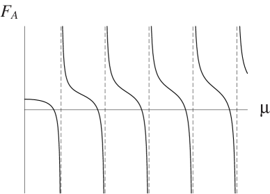
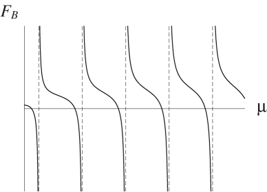
Figure 2: $F_{A}$ (left) and $F_{B}$ (right), as the function of $\mu$ [see (5.2)–(5.3)], for $\mu\geq 0$, with $\nu=2/3$. The dashed lines are located at $\mu_{m}^{\infty}$ (5.14) for $F_{A}$ and $\bar{\mu}_{m}^{\infty}$ (5.19) for $F_{B}$.

The function $F_{A}$ (5.2) is smooth for $\mu\geq 0$, except at the values

$$\mu_{m}^{\infty}=(\nu+1)+2m,\qquad m=0,1,2,\ldots,$$ (5.14)

where it becomes infinite. More precisely, as is easily checked using the properties of the $\Gamma$-function, $F_{A}(\mu)$ approaches $+\infty$ and $-\infty$ as $\mu$ approaches $\mu_{m}^{\infty}$ from above and from below, respectively. It is positive at $\mu=0$, and it takes the value zero at

$$\mu_{m}^{0}=(2-\nu)+2m,\qquad m=0,1,2,\ldots$$ (5.15)

Note that

$$\mu_{m}^{0}<\mu^{\infty}_{m}<\mu_{m+1}^{0}<\mu_{m+1}^{\infty},\qquad m=0,1,2,\ldots$$ (5.16)

It can be shown (see Appendix C) that $F_{A}$ is strictly monotonically decreasing for $\mu\in[0,\mu_{0}^{\infty})$ as well as for $\mu\in(\mu_{m}^{\infty},\mu_{m+1}^{\infty})$ for any $m\geq 0$.

Since the constant on the right hand side of (5.2) is finite, we conclude from the above that (5.2) admits a unique solution in the range $(\mu_{m}^{\infty},\mu_{m+1}^{\infty})$ (5.14) for any $m\geq 0$. There is an additional solution in the range $[0,\mu_{0}^{\infty})$ if

$$F_{A}(0)=\frac{|\Gamma(\frac{1+\nu}{2})|^{2}}{|\Gamma(\frac{2-\nu}{2})|^{2}}\geq\frac{\Gamma(\nu+\frac{1}{2})}{\Gamma(-\nu+\frac{3}{2})}\tan\frac{\alpha\pm\beta}{2}.$$ (5.17)

Let us sketch the analogous description of the function $F_{B}(\mu)$ for $\mu\geq 0$. As is readily verified, $F_{B}(\mu)$ changes sign from positive to negative as $\mu$ passes through the zero locations given by

$$\bar{\mu}_{0}^{0}=|1-\nu|,\quad\bar{\mu}_{m}^{0}=(1-\nu)+2m,\qquad m=1,2,\ldots.$$ (5.18)

It becomes $+\infty$ and $-\infty$ as it approaches

$$\bar{\mu}_{m}^{\infty}=\nu+2m,\qquad m=0,1,2,\ldots$$ (5.19)

from above and from below, respectively. We have

$$\bar{\mu}_{m}^{0}<\bar{\mu}_{m}^{\infty}<\bar{\mu}_{m+1}^{0}<\bar{\mu}_{m+1}^{\infty},\qquad m=0,1,2,\ldots.$$ (5.20)

Similarly to the case of $F_{A}$, one can prove that $F_{B}$ is strictly monotonically decreasing for $\mu\in[0,\bar{\mu}_{0}^{\infty})$ as well as for $\mu\in(\bar{\mu}_{m}^{\infty},\bar{\mu}_{m+1}^{\infty})$ for any $m\geq 0$.

As a consequence of the shape of $F_{B}$, for any finite constant on the right hand side, (5.3) has a unique solution in the range $(\bar{\mu}_{m}^{\infty},\bar{\mu}_{m+1}^{\infty})$ (5.19) for any $m\geq 0$. There is an additional solution in the range $[0,\bar{\mu}_{0}^{\infty})$ if

$$\ F_{B}(0)=\frac{|\Gamma(\frac{\nu}{2})|^{2}}{|\Gamma(\frac{1-\nu}{2})|^{2}}\geq\frac{\Gamma(\nu+\frac{1}{2})}{\Gamma(-\nu+\frac{3}{2})}\tan\frac{\alpha\pm\beta}{2}.$$ (5.21)

5.3 Type 2 eigenvalues

The formula of the function $F_{2}$ in (5.4) is rather complicated for general $U$, for this reason we shall be content with some remarks on the generic properties of the type 2 eigenvalues.

As an illustration, let us first investigate the equation of type 2 non-positive eigenvalues,

$$F_{2}({\mathrm{i}}x)=\pm\frac{1}{2},\qquad x\geq 0,$$ (5.22)

in the special case $\alpha:=-\frac{\pi}{2}$. Under this assumption $F_{2}({\mathrm{i}}x)$ simplifies as

$$F_{2}({\mathrm{i}}x)=\frac{1}{\sin\beta}\left(\frac{\cosh\pi x}{|\cos\pi\nu|}+\frac{\cos\beta}{(6\nu-3)}\left[a_{1}b_{1}+a_{2}b_{2}\right]({\mathrm{i}}x)\right).$$ (5.23)

We see from (4.73) that $a_{k}({\mathrm{i}}x)b_{k}({\mathrm{i}}x)>0$ for $k=1,2$, and therefore

$$F_{2}({\mathrm{i}}x)\geq\frac{1}{\sin\beta|\cos\pi\nu|}>1\qquad\hbox{if}\qquad 0<\beta\leq\frac{\pi}{2}=-\alpha.$$ (5.24)

Thus $M^{U}$ does not admit non-positive type 2 eigenvalues for these choices of the parameters, which include the explicitly solvable case $\beta=-\alpha=\frac{\pi}{2}$ for which $U=\sigma_{1}$. On the contrary, if $\beta>\frac{\pi}{2}=-\alpha$ and $\beta$ is near enough to $\frac{\pi}{2}$, then we have

$$F_{2}(0)>1\qquad\hbox{and}\qquad\lim_{x\to\infty}F_{2}({\mathrm{i}}x)=-\infty,$$ (5.25)

which implies the existence of at least 2 negative eigenvalues of $M^{U}$ for the corresponding $U$ (3.18). The second relation in (5.25) holds since for large $x$ the term $a_{2}({\mathrm{i}}x)b_{2}({\mathrm{i}}x)$ dominates $F_{2}$, unless it is multiplied by zero, as is easily seen from (5.12).

The above example shows that, like in the type 1 case, the existence or non-existence of type 2 negative eigenvalues depends on the choice of the parameters $\alpha,\beta$. One can check that $\lim_{x\to\infty}|F_{2}({\mathrm{i}}x)|=\infty$ always holds, and hence any choice leading to $|F_{2}(0)|<\frac{1}{2}$ guarantees the existence of such eigenvalues. It is also clear that there can be only finitely many negative eigenvalues, the maximal number we found in numerical examples is four.

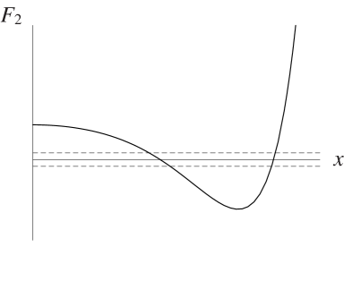
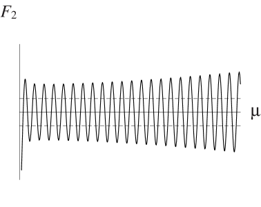
Figure 3: $F_{2}(\mu)$, for imaginary values of $\mu={\mathrm{i}}x$ (left) and for real values of $\mu$ (right). The dashed lines lie at $\pm\frac{1}{2}$. For the left figure, $\nu=\frac{21}{20}$, $\alpha=\frac{11}{20}\pi$ and $\beta=\frac{2}{20}\pi$, a case when the number of solutions of (5.4) is four. For the right figure, the parameters $\nu=\frac{1001}{1000}$, $\alpha=\frac{3}{10}\pi$, and $\beta=\frac{715}{1000}\pi$ are chosen so that the plot exhibits the behaviour of each of the three terms of $F_{2}$ in (5.4). Initially, the rapidly decreasing middle term dominates, then the constant amplitude first term rules, and for larger values the third term gradually becomes the most significant one. Each term oscillates with the same frequency.

Since the multiplicity of the $2$-dimensional representations of $D_{6}$ in $L^{2}(S^{1})$ is obviously infinite, $M^{U}$ has infinitely many type 2 positive eigenvalues. We can understand the approximate behaviour of the solutions of (5.4) for large positive $\mu$ by using the relation (for any real $y$)

$$\lim_{\mu\to\infty}\Gamma(y-\mu)\Gamma(y+\mu)(y+\mu)^{1-2y}\sin\pi(\mu+1-y)=\pi.$$ (5.26)

Since $\nu>\frac{1}{2}$, this implies by (4.73) that $a_{1}(\mu)b_{1}(\mu)$ tends to zero as $\mu\to\infty$, and $a_{2}(\mu)b_{2}(\mu)$ asymptotically equals to a constant multiple of the function

$$f_{2}(\mu):=(1-\nu+\mu)^{2\nu-1}\sin\pi(\mu+\nu).$$ (5.27)

If $(\cos\alpha+\cos\beta)\neq 0$, we thus obtain from (5.4) that $F_{2}(\mu)$ can be approximated by a constant multiple of $f_{2}(\mu)$ as $\mu\to\infty$. Therefore, for large enough $\mu$, there exist two solutions of $|F_{2}(\mu)|=\frac{1}{2}$ between any two consecutive extrema of the function $f_{2}(\mu)$, and actually these solutions lie near to the zeroes of $f_{2}$. If $(\cos\alpha+\cos\beta)=0$, then the first term of $F_{2}$ (5.4) is the dominant one. If $\cos\alpha=\cos\beta=0$, then only this term remains, and we can find the eigenvalues explicitly as discussed in Section 7. If desired, one could derive more precise asymptotic estimates for the solutions of (5.4) by developing the above arguments further. The behaviour of $F_{2}$ near to $\mu=0$ can be rather complicated in general (see Figure 3).

5.4 On the lower-boundedness of the energy as a condition on $U$

We have seen that $M^{U}$ admits, in addition to its infinitely many non-negative eigenvalues, a finite number of negative eigenvalues, too, for certain values of the parameters $\alpha,\beta$ of $U$ (3.18). This result is important, since — as we shall demonstrate in Section 6 — the existence of a negative eigenvalue of $M^{U}$ implies that the energy spectrum of the model (i.e., the spectrum of ${\hat{H}}_{rel}$ (2.3)) is not bounded from below. These cases are to be excluded in hypothetical physical applications. It is complicated to precisely control the conditions for the non-existence of negative eigenvalues of $M^{U}$, but there are certainly cases for which this occurs. For example, if $\alpha=-\frac{\pi}{2}$ and $0<\beta<\frac{\pi}{2}$, then $\tan\frac{\alpha\pm\beta}{2}<0$, and thus neither the inequalities (5.6), (5.7) nor the corresponding equalities can be satisfied. Together with (5.24) this implies that the spectrum of $M^{U}$ is positive for these choices of the parameters of $U$ (3.18). The same holds, for instance, for the explicitly solvable cases $U=\pm{\bf 1}_{2},\pm\sigma_{1}$.

Next, we present a stability result concerning the positivity of the spectrum of $M^{U}$. Suppose that all eigenvalues of $M^{U}$ are positive for some $U=U(\alpha_{0},\beta_{0})$ and the parameters $(\alpha_{0},\beta_{0})$ are generic in the sense that they satisfy the following inequalities:

$$|\tan\frac{\alpha_{0}\pm\beta_{0}}{2}|<\infty,\quad\sin\beta_{0}\neq 0,\quad(\cos\alpha_{0}+\cos\beta_{0})\neq 0.$$ (5.28)

Then it can be proven that $M^{U}$ with $U(\alpha,\beta)$ (3.18) has only positive eigenvalues for any parameters $(\alpha,\beta)$ near enough to $(\alpha_{0},\beta_{0})$.

To verify the above statement, we first observe that neither any of the inequalities in (5.6), (5.7) nor the corresponding equalities can hold for $(\alpha,\beta)$ near to $(\alpha_{0},\beta_{0})$ by continuity. Therefore all type 1 eigenvalues must be positive for such parameters. To exclude the possibility of type 2 non-positive eigenvalues, which would arise from the solutions of (5.22), notice that $F_{2}$ (5.4) can be written in the form

$$F_{2}({\mathrm{i}}x,\alpha,\beta)=e^{\pi x}\left[\kappa_{0}(\alpha,\beta)K_{0}(x)+\kappa_{-}(\alpha,\beta)x^{1-2\nu}K_{-}(x)+\kappa_{+}(\alpha,\beta)x^{2\nu-1}K_{+}(x)\right],$$ (5.29)

where the functions $K_{a}$ satisfy

$$K_{a}(x)>0\quad\forall x\geq 0,\qquad\lim_{x\to\infty}K_{a}(x)=1\qquad(\forall a\in\{0,\pm\}).$$ (5.30)

We see from (4.73) and (5.12) that the above relations are valid with

$$K_{0}(x)=2e^{-\pi x}\cosh\pi x,\quad K_{-}(x)=\frac{2\pi x^{2\nu-1}e^{-\pi x}}{|\Gamma(\nu+{\mathrm{i}}x)|^{2}},\quad K_{+}(x)=\frac{2\pi x^{1-2\nu}e^{-\pi x}}{|\Gamma(1-\nu+{\mathrm{i}}x)|^{2}}$$ (5.31)

and

$$\kappa_{0}(\alpha,\beta)=\frac{1}{2\cos\pi\nu}\frac{\sin\alpha}{\sin\beta},$$

$$\kappa_{-}(\alpha,\beta)=\frac{\Gamma^{2}(\nu+\frac{1}{2})2^{2(\nu-1)}}{\pi(2\nu-1)}\frac{\cos\beta-\cos\alpha}{\sin\beta},$$

$$\kappa_{+}(\alpha,\beta)=\frac{\Gamma^{2}(\frac{3}{2}-\nu)2^{-2\nu}}{\pi(2\nu-1)}\frac{\cos\beta+\cos\alpha}{\sin\beta}.$$ (5.32)

Let us assume that (5.28) is satisfied and $\kappa_{+}(\alpha_{0},\beta_{0})>0$ (the case of the other sign is similar). We can choose a neighbourhood $V_{1}$ of $(\alpha_{0},\beta_{0})$ and constants $\gamma_{a}>0$ so that

$$\kappa_{+}(\alpha,\beta)>\gamma_{+},\quad|\kappa_{0}(\alpha,\beta)|<\gamma_{0},\quad|\kappa_{-}(\alpha,\beta)|<\gamma_{-},\qquad\forall(\alpha,\beta)\in V_{1}.$$ (5.33)

Then we fix some $x_{0}>0$ for which

$$F_{2}({\mathrm{i}}x,\alpha,\beta)\geq e^{\pi x}\left[\gamma_{+}x^{2\nu-1}K_{+}(x)-\gamma_{0}K_{0}(x)-\gamma_{-}x^{1-2\nu}K_{-}(x)\right]>1,\qquad\forall x>x_{0}$$ (5.34)

and $\forall(\alpha,\beta)\in V_{1}$. This ensures that there is no solution of (5.22) for $x>x_{0}$. Since $K_{0}(x)$ and $x^{\pm(2\nu-1)}K_{\pm}(x)$ are bounded on $[0,x_{0}]$, for any $\epsilon>0$ we can find a neighbourhood $V_{2}$ of $(\alpha_{0},\beta_{0})$ so that

$$|F_{2}({\mathrm{i}}x,\alpha,\beta)-F_{2}({\mathrm{i}}x,\alpha_{0},\beta_{0})|\leq\epsilon\qquad\hbox{if}\qquad(\alpha,\beta)\in V_{2},\quad 0\leq x\leq x_{0}.$$ (5.35)

By choosing $\epsilon$ appropriately, for instance in such a way that

$$F_{2}(x,\alpha_{0},\beta_{0})-\frac{1}{2}\geq 2\epsilon\quad\hbox{for}\quad 0\leq x\leq x_{0},$$ (5.36)

we conclude that (5.22) has no solution if $(\alpha,\beta)\in V_{1}\cap V_{2}$. This implies the stability result that we wanted to prove.

We can establish a counterpart of the above stability result concerning the ‘impermissible’ boundary conditions as well, for which negative eigenvalues of the angular Hamiltonian exist. Namely, if $M^{U}$ has one or more negative eigenvalues, then generically this property is stable under arbitrary small perturbations of $U$ in (3.18). Indeed, this is the case obviously if $M^{U}$ admits a type 1 negative eigenvalue or a type 2 negative eigenvalue which is generic in the sense that it arises from the graph of $x\mapsto|F_{2}({\mathrm{i}}x)|$ properly intersecting, not just touching, the horizontal line located at $\frac{1}{2}$.

6 The radial Hamiltonian

Recall from (1.7) that, at the formal level, the radial Hamiltonian reads

$$H_{r,\lambda}=-\frac{d^{2}}{dr^{2}}-\frac{1}{r}\frac{d}{dr}+\frac{3}{8}\omega^{2}r^{2}+\frac{\lambda}{r^{2}}.$$ (6.1)

After having characterized the qualitative features of the eigenvalues $\lambda=(3\mu)^{2}$ of $M^{U}$, we below analyze the energy levels of the relative motion of the three particle Calogero system defined by the eigenvalues of the possible self-adjoint versions of the radial Hamiltonian.

Since $H_{r,\lambda}$ has to be self-adjoint on a domain in $L^{2}({\bf R}_{+},rdr)$, it is more convenient to deal with the equivalent operator

$${\cal H}_{r,\lambda}:=\sqrt{r}\circ H_{r,\lambda}\circ\frac{1}{\sqrt{r}}=-\frac{d^{2}}{dr^{2}}+\frac{3}{8}\omega^{2}r^{2}+\frac{\lambda-\frac{1}{4}}{r^{2}},$$ (6.2)

which must be self-adjoint on a corresponding domain in $L^{2}({\bf R}_{+},dr)$. It is easy to check that, for any eigenvalue, both of the two independent eigenfunctions of the differential operator ${\cal H}_{r,\lambda}$ are locally square integrable around $r=0$ if and only if $\lambda<1$. For this reason [7, 8, 9], ${\cal H}_{r,\lambda}$ admits inequivalent choices of self-adjoint domains if and only if $\lambda<1$. It follows from general theorems, collected in Appendix A from [7], that any self-adjoint version of ${\cal H}_{r,\lambda}$ possesses pure discrete spectrum.

If $\lambda\geq 1$, then the unique self-adjoint domain of ${\cal H}_{r,\lambda}$ consists of those complex functions $\rho$ on ${\bf R}_{+}$ for which $\rho$ and $\rho^{\prime}$ are absolutely continuous away from $r=0$ and both $\rho$ and ${\cal H}_{r,\lambda}\rho$ belong to $L^{2}({\bf R}_{+},dr)$. It is straightforward to show that the spectrum is given by the eigenvalues

$$E_{m,\lambda}=2c(2m+1+\sqrt{\lambda}),\quad c:=\sqrt{\frac{3}{8}}\omega,\quad m=0,1,2,\ldots,$$ (6.3)

with the corresponding eigenfunctions

$$\rho_{m,\lambda}(r)=r^{\frac{1}{2}+\sqrt{\lambda}}e^{-\frac{1}{2}cr^{2}}L_{m}^{\sqrt{\lambda}}(cr^{2}),$$ (6.4)

where $L_{m}^{\sqrt{\lambda}}$ is the (generalized) Laguerre polynomial [20], $\sqrt{\lambda}\geq 1$. This result is contained, for example, in [1, 4].

From now on we consider the case

$$\lambda<1.$$ (6.5)

Let $\varphi_{1}$ and $\varphi_{2}$ be two independent real eigenfunctions of ${\cal H}_{r,\lambda}$ associated with an arbitrary real eigenvalue. In fact (see [8, 16]), in addition to the same properties they have for $\lambda\geq 1$, the functions $\rho$ in a self-adjoint domain of ${\cal H}_{r,\lambda}$ must now also satisfy a boundary condition of the following form:

$$\frac{W[\rho,\varphi_{1}]_{0+}}{W[\rho,\varphi_{2}]_{0+}}=\kappa(\lambda),$$ (6.6)

where $\kappa(\lambda)$ is a real number or is infinity. Here $\kappa(\lambda)=0$ means that $W[\rho,\varphi_{1}]_{0+}=0$, and similarly $W[\rho,\varphi_{2}]_{0+}=0$ is required if $\kappa(\lambda)$ is infinite. Our notation emphasizes that one can in principle choose different constants on the right hand side of (6.6) for different $\lambda$. We remark that the condition (6.6) can be regarded as a special case of the boundary conditions of the form in (3.14), where one restricts to the positive side of the singular point $r=0$ of ${\cal H}_{r,\lambda}$ considered on ${\bf R}$ (accordingly $U$ reduces to a phase), prohibiting the particle from going into $r<0$ from $r>0$. With the ‘reference modes’ $\varphi_{k}$ fixed subsequently, the self-adjoint radial Hamiltonian specified by condition (6.6) is denoted as ${\cal H}_{r,\lambda,\kappa(\lambda)}$. (In the notation used in (2.3), one may substitute ${\hat{H}}_{r,\lambda,\kappa(\lambda)}:=\frac{1}{\sqrt{r}}\circ{\cal H}_{r,\lambda,\kappa(\lambda)}\circ\sqrt{r}$ for ${\hat{H}}_{r,\lambda}$.)

In order to determine the spectrum of ${\cal H}_{r,\lambda,\kappa(\lambda)}$, we first write down the solutions of

$${\cal H}_{r,\lambda}\rho=E\rho$$ (6.7)

for any real number $E$. To do this, it is convenient to introduce

$$\sigma:=cr^{2},\qquad\xi:=\frac{E}{4c}-\frac{\sqrt{\lambda}+1}{2}$$ (6.8)

with $c$ given in (6.3). Then one can check that, if $\lambda\neq 0$, two independent solutions of (6.7) are provided by the functions

$$\rho_{E,1}(r)=\sigma^{\frac{1}{2}(\frac{1}{2}+\sqrt{\lambda})}e^{-\frac{1}{2}\sigma}\Phi(-\xi,\sqrt{\lambda}+1,\sigma),$$

$$\rho_{E,2}(r)=\sigma^{\frac{1}{2}(\frac{1}{2}-\sqrt{\lambda})}e^{-\frac{1}{2}\sigma}\Phi(-\xi-\sqrt{\lambda},1-\sqrt{\lambda},\sigma),$$ (6.9)

where $\Phi(a,b,z)$ is the confluent hypergeometric function, also called Kummer’s function. Here, as before, we insist on the convention that either $\sqrt{\lambda}=3\mu\geq 0$ or its imaginary part is positive. Up to a multiplicative factor, there is a unique linear combination of the functions in (6.9) that lies in $L^{2}({\bf R}_{+},dr)$, given by

$$\rho_{E}=\frac{\Gamma(1-\sqrt{\lambda})}{\Gamma(-\xi-\sqrt{\lambda})}\rho_{E,1}-\frac{\Gamma(1+\sqrt{\lambda})}{\Gamma(-\xi)}\rho_{E,2}.$$ (6.10)

In fact, with an irrelevant factor $C(\sqrt{\lambda})$, one has

$$\rho_{E}(r)=C(\sqrt{\lambda})\sigma^{\frac{1}{2}(\frac{1}{2}+\sqrt{\lambda})}e^{-\frac{1}{2}\sigma}U(-\xi,1+\sqrt{\lambda},\sigma),$$ (6.11)

where the function $U$ satisfies $U(\xi,1+\sqrt{\lambda},\sigma)=\sigma^{\xi}[1+O(\sigma^{-1})]$ as $\sigma\to\infty$ (see eq. 13.1.8 in [21]). This guarantees the square integrability of $\rho_{E}$. For $E$ to belong to the spectrum of ${\cal H}_{r,\lambda,\kappa(\lambda)}$, $\rho_{E}$ must satisfy the boundary condition (6.6).

Let us now suppose that

$$0<\lambda<1.$$ (6.12)

In this case the $\rho_{E,k}$ are real functions, and we fix our reference modes to be

$$\varphi_{k}:=\rho_{E_{0},k}$$ (6.13)

with some arbitrary real $E_{0}$. For arbitrary $E$ and $E_{0}$, an easy calculation yields

$$W[\rho_{E,k},\rho_{E_{0},l}]_{0+}:=\lim_{r\to 0}\left(\rho_{E,k}\frac{d\rho_{E_{0},l}}{dr}-\rho_{E_{0},l}\frac{d\rho_{E,k}}{dr}\right)(r)=-2\epsilon_{k,l}\sqrt{\lambda}\sqrt{c},$$ (6.14)

where $\epsilon_{k,l}$ is the usual alternating tensor. Therefore we find that

$$\frac{W[\rho_{E},\varphi_{1}]_{0+}}{W[\rho_{E},\varphi_{2}]_{0+}}=\frac{\Gamma(1+\sqrt{\lambda})\Gamma(-\xi-\sqrt{\lambda})}{\Gamma(1-\sqrt{\lambda})\Gamma(-\xi)}.$$ (6.15)

By substituting back $\xi$ (6.8), we obtain the following condition that determines the eigenvalues of ${\cal H}_{r,\lambda,\kappa(\lambda)}$ under (6.12):

$$F_{\lambda}(\epsilon):=\frac{\Gamma(-\epsilon+\frac{1-\sqrt{\lambda}}{2})}{\Gamma(-\epsilon+\frac{1+\sqrt{\lambda}}{2})}=-\frac{\Gamma(-\sqrt{\lambda})}{\Gamma(\sqrt{\lambda})}\kappa(\lambda)\qquad\hbox{with}\qquad\epsilon:=\frac{E}{4c}.$$ (6.16)

Next, we analyze the shape of the function $F_{\lambda}$, which is illustrated by Figure 4.

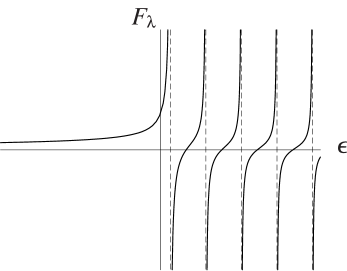
Figure 4: $F_{\lambda}$, as the function of $\epsilon$ [see (6.16)], for $\lambda=1/5$. The dashed lines, where the function diverges, are located at $\epsilon_{m}^{\infty}$ (6.18).

Let us start by observing that $F_{\lambda}$ has zeroes at

$$\epsilon_{m}^{0}=\frac{1+\sqrt{\lambda}}{2}+m,\qquad\forall m=0,1,2,\ldots$$ (6.17)

and it becomes $\pm\infty$ at $\epsilon_{m}^{\infty}\mp 0$ for

$$\epsilon_{m}^{\infty}=\frac{1-\sqrt{\lambda}}{2}+m,\qquad\forall m=0,1,2,\ldots$$ (6.18)

By considering

$$\frac{F_{\lambda}^{\prime}(\epsilon)}{F_{\lambda}(\epsilon)}=\psi(-\epsilon+\frac{1+\sqrt{\lambda}}{2})-\psi(-\epsilon+\frac{1-\sqrt{\lambda}}{2})$$ (6.19)

with the notation (5.9), wee see immediately that for

$$-\infty<\epsilon<\epsilon_{0}^{\infty}$$ (6.20)

$F_{\lambda}(\epsilon)>0$ and $F_{\lambda}^{\prime}(\epsilon)>0$. This and the asymptotics of $F_{\lambda}$ imply that $F_{\lambda}(\epsilon)$ monotonically increases from $0$ to $+\infty$ as $\epsilon$ varies from $-\infty$ to $\epsilon_{0}^{\infty}$. If $\epsilon>\epsilon_{0}^{\infty}$, we use the reflection formula (C.2) for $\psi$ to write

$$\frac{F_{\lambda}^{\prime}(\epsilon)}{F_{\lambda}(\epsilon)}=\left[\psi(\epsilon+\frac{1-\sqrt{\lambda}}{2})-\psi(\epsilon+\frac{1+\sqrt{\lambda}}{2})\right]+\pi\left[\cot\pi(\epsilon+\frac{1-\sqrt{\lambda}}{2})-\cot\pi(\epsilon+\frac{1+\sqrt{\lambda}}{2})\right].$$ (6.21)

We have

$$\epsilon_{m}^{\infty}<\epsilon_{m}^{0}<\epsilon_{m+1}^{\infty},\qquad\forall m=0,1,2,\ldots$$ (6.22)

If

$$\epsilon_{m}^{\infty}<\epsilon<\epsilon_{m}^{0},$$ (6.23)

then both differences in the square brackets in (6.21) are negative. Since under (6.23) $F_{\lambda}(\epsilon)<0$, it follows that $F_{\lambda}$ is monotonically increasing in this domain. If

$$\epsilon_{m}^{0}<\epsilon<\epsilon_{m+1}^{\infty},$$ (6.24)

then $F_{\lambda}(\epsilon)>0$ and the differences in (6.21) have opposite signs. We can show that $F_{\lambda}^{\prime}(\epsilon)>0$ by using the integral formulae (C.12) and (C.13) in the same way as in Appendix C, which proves that $F_{\lambda}$ is increasing in this domain as well.

Supposing that $\kappa(\lambda)\notin\{0,\infty\}$, it is clear from the shape of the function $F_{\lambda}$ that there exists precisely one positive eigenvalue, $\frac{E}{4c}$, in each interval $(\epsilon_{m}^{\infty},\epsilon_{m+1}^{\infty})$ for any non-negative integer $m$. Moreover, one obtains at most one negative eigenvalue, which occurs precisely if

$$F_{\lambda}(0)=\frac{\Gamma(\frac{1-\sqrt{\lambda}}{2})}{\Gamma(\frac{1+\sqrt{\lambda}}{2})}>-\frac{\Gamma(-\sqrt{\lambda})}{\Gamma(\sqrt{\lambda})}\kappa(\lambda)>0.$$ (6.25)

There is also a non-negative eigenvalue in $[0,\epsilon_{0}^{\infty})$ if $F_{\lambda}(0)\leq-\frac{\Gamma(-\sqrt{\lambda})}{\Gamma(\sqrt{\lambda})}\kappa(\lambda)$.

The eigenvalue equation (6.16) is explicitly solvable if $\kappa(\lambda)=0$ or $\kappa(\lambda)=\infty$. In the former case the eigenvalues have the same form as in (6.3), and the corresponding eigenfunction reduces to $\rho_{E,1}$ in (6.9), which has the same form as (6.4) up to an irrelevant constant. If $\kappa(\lambda)=\infty$, then we find the eigenvalues

$$\tilde{E}_{m,\lambda}=2c(2m+1-\sqrt{\lambda}),\qquad m=0,1,2,\ldots$$ (6.26)

Under $E=\tilde{E}_{m,\lambda}$, $\rho_{E}$ (6.10) is proportional to $\rho_{E,2}$, which (up to another irrelevant factor) gives the eigenfunction

$$\tilde{\rho}_{m,\lambda}(r)=r^{\frac{1}{2}-\sqrt{\lambda}}e^{-\frac{1}{2}cr^{2}}L_{m}^{-\sqrt{\lambda}}(cr^{2}),$$ (6.27)

Note that all energy levels are positive in these cases.

Our spectral condition (6.16) is consistent with the result in [10], where the inequivalent quantizations of the radial Hamiltonian $H_{r,\lambda}$ (1.7) were considered by using a different method, with $0<\lambda<1$ taken from the eigenvalues of two special self-adjoint versions of the angular Hamiltonian $H_{\Omega}$ (1.6) that are well-understood for any $N$ due to Calogero [2]. In our $N=3$ case-study those correspond to $M^{U}$ with $U=-{\bf 1}_{2}$ or $U={\bf 1}_{2}$.

Let us now deal with the case when

$$\sqrt{\lambda}=3\mu={\mathrm{i}}x\quad\hbox{with some}\quad x>0.$$ (6.28)

Then the functions $\rho_{E,k}$ are complex, and their real and imaginary parts are also solutions of (6.7). We choose our reference modes to be (up to a factor) the real and imaginary parts of $\rho_{E_{0},1}$ for some real $E_{0}$. Explicitly, with $\xi_{0}=\frac{E_{0}}{4c}-\frac{{\mathrm{i}}x+1}{2}$, we define

$$\varphi_{1}(r):=r^{\frac{1}{2}}e^{-\frac{1}{2}\sigma}\left[\Re\Phi(-\xi_{0},1+{\mathrm{i}}x,\sigma)\cos(x\log r)-\Im\Phi(-\xi_{0},1+{\mathrm{i}}x,\sigma)\sin(x\log r)\right]\qquad\quad$$

$$\varphi_{2}(r):=r^{\frac{1}{2}}e^{-\frac{1}{2}\sigma}\left[\Re\Phi(-\xi_{0},1+{\mathrm{i}}x,\sigma)\sin(x\log r)+\Im\Phi(-\xi_{0},1+{\mathrm{i}}x,\sigma)\cos(x\log r)\right].$$ (6.29)

These eigenfunctions of ${\cal H}_{r,\lambda}$ are independent, since we find

$$W[\varphi_{1},\varphi_{2}](r)=\lim_{r\rightarrow 0+}W[\varphi_{1},\varphi_{2}](r)=x.$$ (6.30)

One also readily calculates that

$$\lim_{r\rightarrow 0+}W[\rho_{E,1},\varphi_{1}](r)=-{\mathrm{i}}xc^{\frac{1}{2}({\frac{1}{2}+{\mathrm{i}}x})}$$

$$\lim_{r\rightarrow 0+}W[\rho_{E,2},\varphi_{1}](r)={\mathrm{i}}xc^{\frac{1}{2}({\frac{1}{2}-{\mathrm{i}}x})}$$

$$\lim_{r\rightarrow 0+}W[\rho_{E,1},\varphi_{2}](r)=xc^{\frac{1}{2}({\frac{1}{2}+{\mathrm{i}}x})}$$

$$\lim_{r\rightarrow 0+}W[\rho_{E,2},\varphi_{2}](r)=xc^{\frac{1}{2}({\frac{1}{2}-{\mathrm{i}}x})}.$$ (6.31)

By inserting these into (6.6) for $\rho=\rho_{E}$ (6.10), we obtain the following eigenvalue equation:

$$\cot\arg\left(c^{\frac{1}{2}{\mathrm{i}}x}\Gamma(1-{\mathrm{i}}x)\Gamma(-\epsilon+\frac{1+{\mathrm{i}}x}{2})\right)=-\kappa(\lambda)\qquad(\epsilon=\frac{E}{4c}).$$ (6.32)

Equivalently, we have to solve

$$\frac{\Re\left(c^{\frac{1}{2}{\mathrm{i}}x}\Gamma(1-{\mathrm{i}}x)\Gamma(-\epsilon+\frac{1+{\mathrm{i}}x}{2})\right)}{\Im\left(c^{\frac{1}{2}{\mathrm{i}}x}\Gamma(1-{\mathrm{i}}x)\Gamma(-\epsilon+\frac{1+{\mathrm{i}}x}{2})\right)}=-\kappa(\lambda).$$ (6.33)

Because of the shape of the potential in (6.2), one expects to find infinitely many solutions for $\epsilon$ around $+\infty$ as well as around $-\infty$.

Indeed, we can easily prove that the accumulation points of the spectrum of ${\cal H}_{r,\lambda,\kappa(\lambda)}$ are precisely $\pm\infty$. For this purpose, it is advantageous to rewrite (6.32) as

$$\Omega(\epsilon,x):=\arg\Gamma(-\epsilon+\frac{1}{2}+\frac{{\mathrm{i}}x}{2})=\vartheta(x,\kappa(\lambda),c)\quad\hbox{mod}\,\,\pi,$$ (6.34)

where

$$\vartheta(x,\kappa(\lambda),c)=\mbox{arccot}(-\kappa(\lambda))-\arg\Gamma(1-{\mathrm{i}}x)-\frac{x}{2}\log c.$$ (6.35)

In (6.34) we can take $\Omega(\epsilon,x)$ to be the smooth function of $\epsilon\in{\bf R}$ defined by

$$\Omega(\epsilon,x):=\ \arg\Gamma(\frac{1}{2}+\frac{{\mathrm{i}}x}{2})+\int_{0}^{\epsilon}dy\,\omega(y,x),$$ (6.36)

where the ambiguity in $\arg\Gamma(\frac{1}{2}+\frac{{\mathrm{i}}x}{2})$ is fixed arbitrarily and

$$\omega(y,x):=\frac{d}{dy}\arg\Gamma(-y+\frac{1}{2}+\frac{{\mathrm{i}}x}{2})=\frac{1}{2{\mathrm{i}}}\left[\psi(-y+\frac{1}{2}-\frac{{\mathrm{i}}x}{2})-\psi(-y+\frac{1}{2}+\frac{{\mathrm{i}}x}{2})\right].$$ (6.37)

It follows by means of (5.10) that $\omega(y,x)<0$, and one sees with the help of the asymptotic expansion of $\psi$ and (6.36) (or directly from the asymptotic expansion of $\Gamma$) that $\lim_{\epsilon\to\pm\infty}\Omega(\epsilon,x)=\mp\infty$. Therefore $\Omega(\epsilon,x)$ decreases monotonically from $+\infty$ to $-\infty$ as $\epsilon$ runs through the real axis. This implies that the set of solutions of (6.34) is bounded neither from below nor from above, and there are finitely many solutions in any finite interval.

In the foregoing derivation we assumed that $\kappa(\lambda)\neq 0$ and $\kappa(\lambda)\neq\infty$, but the conclusion remains valid for these special values, too, as one can confirm by inspection of the respective conditions $W[\rho_{E},\varphi_{1}]_{0+}=0$ and $W[\rho_{E},\varphi_{2}]_{0+}=0$.

Since for $\lambda<0$ the energy spectrum is not bounded from below, in physical applications one has to exclude those connection matrices $U$ for which the angular Hamiltonian $M^{U}$ possesses a negative eigenvalue.

7 Explicitly solvable cases

We illustrate our inequivalent quantizations of the $N=3$ Calogero model by considering a few special cases which can be solved explicitly. Recall that our inequivalent quantizations are specified by the parameter $\kappa(\lambda)$ (to each $\lambda<1$) for the radial part (6.6) and the parameters in $U$ (3.18) for the angular part. In this section $\lambda$ will always be positive, and for simplicity we adopt the choice $\kappa(\lambda)=0$ for any $0<\lambda<1$. Then the energy eigenvalues and the radial solutions have the form given by (6.3) and (6.4) for all $\lambda>0$. For the angular part, we consider the four cases, $U=-{\bf 1}_{2}$, $U={\bf 1}_{2}$, $U=\sigma_{1}$ and $U=-\sigma_{1}$. We shall see, in particular, that the case $U=\sigma_{1}$ admits a smooth limit for $\nu\to 1$ (i.e., $g\to 0$) in which the system defined by ${\hat{H}}_{rel}$ (2.3) becomes the harmonic oscillator in two dimensions. For $U\neq\sigma_{1}$ the system resulting in the $g\to 0$ limit can be interpreted as the harmonic oscillator plus an extra singular potential in the angular sector, which is supported at the points of ${\cal S}$ (3.5) and manifests itself in the boundary condition.

The spectrum of the angular Hamiltonian for $U=\pm{\bf 1}_{2},\pm\sigma_{1}$ and the energy spectrum for $U=\sigma_{1}$ are summarized by Figure 5 at the end of the section.

7.1 The case $U=-{\bf 1}_{2}$

We begin by the ‘Dirichlet’ case $U=-{\bf 1}_{2}$, which is in fact the standard choice of boundary condition that has been used since the introduction of the model [1]. As $U=-{\bf 1}_{2}$ is one of the separating cases discussed in Section 4.2, we just recall (4.31)–(4.34) for the eigenstates of the angular part. With the eigenvalues, the solutions are

$$\eta_{\mu}^{A}(\phi)=\sum_{k=1}^{6}C_{-}^{k}\eta_{-,\mu}^{k}(\phi),\qquad\mu=2n+1+\nu,$$

$$\eta_{\mu}^{B}(\phi)=\sum_{k=1}^{6}C_{+}^{k}\eta_{+,\mu}^{k}(\phi),\qquad\mu=2n+\nu,$$ (7.1)

for $n=0,1,2,\ldots$. The arbitrary coefficients $C_{\pm}^{k}$, $k=1,2,\ldots,6$ show that all levels have multiplicity 6.

These solutions $\eta_{\mu}^{A}$, $\eta_{\mu}^{B}$ are then combined with the solutions for the radial part $R_{m,\lambda}(r)=r^{-{1\over 2}}\rho_{m,\lambda}(r)$, where $\rho_{m,\lambda}$ is given in (6.4), to form the eigenstates for the entire system governed by ${\hat{H}}_{rel}$. Since $\lambda=(3\mu)^{2}$ is determined by $n$, those states (modulo the normalization constant) may be presented as ($m,n=0,1,2,\ldots$)

$$\Psi^{A}_{mn}(r,\phi)=R_{m,\lambda}(r)\,\eta_{\mu}^{A}(\phi),\qquad E^{A}_{mn}=2c\left(2m+1+3(2n+1+\nu)\right),$$

$$\Psi^{B}_{mn}(r,\phi)=R_{m,\lambda}(r)\,\eta_{\mu}^{B}(\phi),\qquad E^{B}_{mn}=2c\left(2m+1+3(2n+\nu)\right),$$ (7.2)

where $2c=\sqrt{{3\over 2}}\,\omega$; see (6.3).

On account of the multiplicity, one can choose the eigenstate in any particular representation of the exchange-$S_{3}$ (or more generally the $D_{6}$) symmetry group. For example, if we choose $C_{-}^{k}=(-1)^{k-1}C_{-}^{1}$ for $k=2,\ldots,6$, then the resultant state $\eta_{\mu}^{A}$ for the angular part becomes a $(+1)$ eigenstate of all the reflections $\hat{P}_{n}$ and hence it is bosonic. On the other hand, if we choose $C_{-}^{k}=C_{-}^{1}$, then the resultant state $\eta_{\mu}^{A}$ becomes a $(-1)$ eigenstate and hence it is fermionic. In contrast, for $\eta_{\mu}^{B}$ the choice $C_{+}^{k}=(-1)^{k-1}C_{+}^{1}$ makes it fermionic and $C_{+}^{k}=C_{+}^{1}$ makes it bosonic. At this point we recall that the basic solutions $v_{i,\mu}(\phi)$, $i=1,2$, defined in (4.1) are periodic in $\phi$ with period ${\pi\over 3}$ and are symmetric with respect to $\phi={\pi\over 6}$. Thus, if we introduce the sign factors,

$$c(\phi):={{\cos 3\phi}\over{|\cos 3\phi|}},\qquad s(\phi):={{\sin 3\phi}\over{|\sin 3\phi|}},\qquad t(\phi):={{\tan 3\phi}\over{|\tan 3\phi|}},$$ (7.3)

we can express these bosonic and fermionic eigenstates concisely over $S^{1}\setminus{\cal S}$ in terms of the basic functions. For instance, the bosonic states may be presented as

$$\eta_{\mu}^{A}(\phi)=c(\phi)\,v_{1,\mu}(\phi),\qquad\eta_{\mu}^{B}(\phi)=v_{1,\mu}(\phi),$$ (7.4)

for the levels $\mu$ given, respectively, by (7.1). It is easily confirmed that the sign factor $c(\phi)$ attached in (7.4) takes care of the sign conventions required for $\eta_{-,\mu}^{k}$ together with the choice of the coefficients needed to provide the bosonic states. Similarly, the fermionic states are given by

$$\eta_{\mu}^{A}(\phi)=t(\phi)\,v_{1,\mu}(\phi),\qquad\eta_{\mu}^{B}(\phi)=s(\phi)\,v_{1,\mu}(\phi).$$ (7.5)

For the eigenvalues $\mu$ in (7.1), one may use the relation

$$F\left(-{l\over 2},\,{l\over 2}+\nu,\,\nu+{1\over 2};\,\sin^{2}3\phi\right)={{l!\,\Gamma(2\nu)}\over{\Gamma(l+2\nu)}}\,C_{l}^{\nu}(|\cos 3\phi|)$$ (7.6)

to replace $v_{1,\mu}$ in (7.4) and (7.5) with the Gegenbauer polynomial $C_{l}^{\nu}$. These bosonic and fermionic eigenstates recover the original solutions obtained by Calogero for $N=3$ [1].

7.2 The case $U={\bf 1}_{2}$

The ‘Neumann’ case $U={\bf 1}_{2}$ can be solved analogously to the preceding ‘Dirichlet’ case; eq. (4.31) with (4.35) yields the angular solutions

$$\eta_{\mu}^{A}(\phi)=\sum_{k=1}^{6}C_{-}^{k}\eta_{-,\mu}^{k}(\phi),\qquad\mu=2n+1+(1-\nu),$$

$$\eta_{\mu}^{B}(\phi)=\sum_{k=1}^{6}C_{+}^{k}\eta_{+,\mu}^{k}(\phi),\qquad\mu=|2n+(1-\nu)|,$$ (7.7)

for $n=0,1,2,\ldots$, with arbitrary coefficients $C_{\pm}^{k}$, $k=1,\ldots,6$. The eigenstates and the eigenvalues for the entire system thus read

$$\Psi^{A}_{mn}(r,\phi)=R_{m,\lambda}(r)\,\eta_{\mu}^{A}(\phi),\qquad E^{A}_{mn}=2c\left(2m+1+3(2n+1+(1-\nu))\right),$$

$$\Psi^{B}_{mn}(r,\phi)=R_{m,\lambda}(r)\,\eta_{\mu}^{B}(\phi),\qquad E^{B}_{mn}=2c\left(2m+1+3|2n+(1-\nu)|\right).$$ (7.8)

As in the previous case, the eigenstates can be made bosonic or fermionic by choosing the coefficients $C_{\pm}^{k}$, appropriately. Concise forms for these states are also available as

$$\eta_{\mu}^{A}(\phi)=c(\phi)\,v_{2,\mu}(\phi),\qquad\eta_{\mu}^{B}(\phi)=v_{2,\mu}(\phi),$$ (7.9)

for the bosonic states, and

$$\eta_{\mu}^{A}(\phi)=t(\phi)\,v_{2,\mu}(\phi),\qquad\eta_{\mu}^{B}(\phi)=s(\phi)\,v_{2,\mu}(\phi),$$ (7.10)

for the fermionic states. As before, by using the relation (7.6) with $\nu$ substituted by $1-\nu$, one may replace $v_{2,\mu}$ with the corresponding Gegenbauer polynomial $C_{l}^{1-\nu}$ in the final expression of the solutions.

7.3 The case $U=\sigma_{1}$

The case $U=\sigma_{1}$ is distinguished in the sense that it leads to the free connection condition (i.e., both the wave function and its derivative are continuous) in the limit $\nu\to 1$ where the singularity of the potential disappears. This ‘free’ case is one of the non-separating cases in which the spectrum consists of eigenvalues of both type 1 and type 2 eigenstates. The eigenvalues are determined by the spectral condition (4.55), which now simplifies to

$$-\frac{\cos\pi\mu}{\cos\pi\nu}=\Re(\tau),$$ (7.11)

using that the parameters in (3.18) are ${\cal A}=0$ and ${\cal B}=1$.

For type 1 eigenstates for which $\Re(\tau)=\pm 1$, it is immediate to find the solutions for positive $\mu$. For $\Re(\tau)=1$, these are

$$\mu=2n+1+\nu\quad\hbox{and}\quad\mu=|2n+(1-\nu)|,\qquad n=0,1,2,\ldots,$$ (7.12)

which correspond to the $A_{-}$ and the $B_{+}$ case defined in (4.58) and (4.59) (see also (4.33), (4.37)). Similarly, for $\Re(\tau)=-1$, we obtain

$$\mu=2n+\nu\quad\hbox{and}\quad\mu=2n+1+(1-\nu),\qquad n=0,1,2,\ldots,$$ (7.13)

which correspond to the $B_{-}$ and the $A_{+}$ case. In fact, these are the solutions mentioned in (4.62)–(4.65), which arise since our parameters (3.18) satisfy $e^{i(\alpha+\beta)}=1$ and $e^{i(\alpha-\beta)}=-1$. Thus, the type 1 solutions for the angular part are

$$\eta_{\mu}^{A_{+}}(\phi)=-c(\phi)\,a_{1}(\mu)v_{2,\mu}(\phi),\qquad\mu=2n+1+(1-\nu),$$

$$\eta_{\mu}^{A_{-}}(\phi)=t(\phi)\,a_{2}(\mu)v_{1,\mu}(\phi),\qquad\quad\!\mu=2n+1+\nu,$$

$$\eta_{\mu}^{B_{+}}(\phi)=-b_{1}(\mu)v_{2,\mu}(\phi),\qquad\qquad\mu=|2n+(1-\nu)|,$$

$$\eta_{\mu}^{B_{-}}(\phi)=s(\phi)\,b_{2}(\mu)v_{1,\mu}(\phi).\qquad\quad\mu=2n+\nu.$$ (7.14)

Combining these with the eigenstates for the radial part, we obtain the type 1 eigenfunctions and energy eigenvalues for the entire system ($m,n=0,1,2,\ldots$):

$$\Psi^{++}_{mn}(r,\phi)=R_{m,\lambda}(r)\,\eta_{\mu}^{B_{+}}(\phi),\qquad E^{++}_{mn}=2c\left(2m+1+3|2n+(1-\nu)|\right),$$

$$\Psi^{-+}_{mn}(r,\phi)=R_{m,\lambda}(r)\,\eta_{\mu}^{A_{+}}(\phi),\qquad E^{-+}_{mn}=2c\left(2m+1+3(2n+1+(1-\nu))\right),$$

$$\Psi^{+-}_{mn}(r,\phi)=R_{m,\lambda}(r)\,\eta_{\mu}^{B_{-}}(\phi),\qquad E^{+-}_{mn}=2c\left(2m+1+3(2n+\nu)\right),$$

$$\Psi^{--}_{mn}(r,\phi)=R_{m,\lambda}(r)\,\eta_{\mu}^{A_{-}}(\phi),\qquad E^{--}_{mn}=2c\left(2m+1+3(2n+1+\nu)\right),$$ (7.15)

where the superscripts on $\Psi_{mn}$ specify the $D_{6}$ representation similarly to (4.67). We observe that for $U=\sigma_{1}$ the type 1 eigenstates $\eta_{\mu}^{A_{+}}$, $\eta_{\mu}^{B_{+}}$ are basically the bosonic eigenstates (7.9) admitted under $U={\bf 1}_{2}$, while $\eta_{\mu}^{A_{-}}$, $\eta_{\mu}^{B_{-}}$ are the fermionic eigenstates (7.5) admitted under $U=-{\bf 1}_{2}$.

Next, we turn to type 2 eigenstates for which $\Re(\tau)=\pm{1\over 2}$. Since the spectral condition (7.11) is analogous to the type 1 case, if we use

$$\Delta(\nu):={1\over\pi}\arccos\left(\frac{1}{2}\cos\pi\nu\right),$$ (7.16)

we obtain the solutions,

$$\mu=2n+1+\Delta(\nu)\quad\hbox{and}\quad\mu=2n+(1-\Delta(\nu)),\qquad n=0,1,2,\ldots,$$ (7.17)

for $\Re(\tau)={1\over 2}$, and

$$\mu=2n+\Delta(\nu)\quad\hbox{and}\quad\mu=2n+1+(1-\Delta(\nu)),\qquad n=0,1,2,\ldots,$$ (7.18)

for $\Re(\tau)=-{1\over 2}$. Note that

$${1\over 2}<\Delta(\nu)<{2\over 3},\qquad\Delta(\nu)<\nu$$ (7.19)

for $\nu$ in the range (2.9). We also remark that no solution with $\mu^{2}\leq 0$ is allowed for (7.11) for both type 1 and type 2 eigenstates.

The eigenfunctions associated with the type 2 eigenvalues can be constructed by the procedure of Section 4.3. Namely, one first obtains the eigenvector (4.75) with the aid of the projection operator $\pi_{\tau}(\mu)$ in (4.76). Then, taking into account (4.40) and (4.53), one forms the eigenfunction $\eta_{\mu}(\phi)$ in (4.9) out of the functions $\eta_{\pm,\mu}^{k}(\phi)$. Using the spectral condition (7.11) and $y(\mu)=-4{\mathrm{i}}a_{1}(\mu)a_{2}(\mu)$, $z(\mu)=-4{\mathrm{i}}b_{1}(\mu)b_{2}(\mu)$ for $\pi_{\tau}(\mu)$, and choosing the overall scale factor of the eigenvector appropriately, one arrives at

$$\eta_{\mu,\tau}(\phi)=-{{{\mathrm{i}}q(\mu)}\over{\Im(\tau)}}v_{1,\mu}(\phi)+v_{2,\mu}(\phi),$$ (7.20)

where

$$q(\mu)={{3\cos^{2}\pi\nu}\over{2\pi^{2}}}2^{-2\nu}\,\Gamma(-\nu+{1\over 2})\,\Gamma(-\nu+{3\over 2})\,\Gamma(\nu+\mu)\,\Gamma(\nu-\mu).$$ (7.21)

This is valid for $0<\phi\leq{\pi\over 6}$ in sector 1, and extension to the remaining half of sector 1 can be done by expressing in (7.20) the $v_{i,\mu}$ on $0<\phi\leq\frac{\pi}{6}$ in terms of the functions $\eta_{\pm,\mu}^{1}(\phi)$ defined by (4.5), (4.6), and adopting the resulting formula on the whole sector 1. Subsequent extension to sector $k$ can be made in terms of the rotated functions $\eta_{\pm,\mu}^{k}(\phi)$ defined in (4.7) and the eigenvector for sector $k$ which is given by $\tau^{k-1}$ times the eigenvector for sector 1 (see (4.40) and (4.53)). Note that to each $\mu$ we have two solutions for $\eta_{\mu,\tau}(\phi)$ on account of $\Im(\tau)=\pm{{\sqrt{3}}\over 2}$, implying that each level is indeed doubly degenerate.

To display the above eigenstates and their eigenvalues more systematically, let us use the notation introduced in the paragraph above (4.70) for the states belonging to the different type 2 representations of $D_{6}$. Thus the states $\eta^{(2)}_{\mu,\tau}$ arise for $\Re(\tau)={1\over 2}$ and $\tilde{\eta}^{(2)}_{\mu,\tau}$ for $\Re(\tau)=-{1\over 2}$, that is, for eigenvalues (7.17) and (7.18), respectively. We observe that, like in the case of type 1 states, each of the sets $\{\eta^{(2)}_{\mu,\tau}\}$ and $\{\tilde{\eta}^{(2)}_{\mu,\tau}\}$ can be classified into two distinct series according to the difference in the non-integral part of $\mu$. We introduce the notation $\eta^{(2)-}_{\mu,\tau}$ for the eigenstates (7.20) with $\mu=2n+1+\Delta(\nu)$ and $\eta^{(2)+}_{\mu,\tau}$ for those with $\mu=2n+(1-\Delta(\nu))$, and similarly $\tilde{\eta}^{(2)-}_{\mu,\tau}$ with $\mu=2n+\Delta(\nu)$ and $\tilde{\eta}^{(2)+}_{\mu,\tau}$ with $\mu=2n+1+(1-\Delta(\nu))$. Combining with the solutions for the radial part, and adopting similar notation to specify the entire eigenstates containing the type 2 angular states, we obtain

$$\Psi^{(2)+}_{mn,\tau}(r,\phi)=R_{m,\lambda}(r)\,\eta_{\mu,\tau}^{(2)+}(\phi),\qquad E^{(2)+}_{mn}=2c\left(2m+1+3(2n+(1-\Delta(\nu)))\right),$$

$$\tilde{\Psi}^{(2)+}_{mn,\tau}(r,\phi)=R_{m,\lambda}(r)\,\tilde{\eta}_{\mu,\tau}^{(2)+}(\phi),\qquad\tilde{E}^{(2)+}_{mn}=2c\left(2m+1+3(2n+1+(1-\Delta(\nu))\right),$$

$$\tilde{\Psi}^{(2)-}_{mn,\tau}(r,\phi)=R_{m,\lambda}(r)\,\tilde{\eta}_{\mu,\tau}^{(2)-}(\phi),\qquad\tilde{E}^{(2)-}_{mn}=2c\left(2m+1+3(2n+\Delta(\nu))\right),$$

$$\Psi^{(2)-}_{mn,\tau}(r,\phi)=R_{m,\lambda}(r)\,\eta_{\mu,\tau}^{(2)-}(\phi),\qquad E^{(2)-}_{mn}=2c\left(2m+1+3(2n+1+\Delta(\nu))\right).$$ (7.22)

Note that $\mu$ can be recovered from the energy as $3\mu=\frac{E}{2c}-2m-1$. The energy eigenvalues in (7.15) and (7.22) provide the complete spectrum of the $N=3$ Calogero model defined by the Hamiltonian ${\hat{H}}_{rel}$ (2.3) under the angular boundary condition $U=\sigma_{1}$. We mention that, for any $\nu$, the ground (the lowest energy) state is given by the type 1 state $\Psi^{++}_{00}$ possessing the energy $E^{++}_{00}=2c\left(1+3|1-\nu|\right)$.

Now, let us consider the harmonic oscillator limit $\nu\to 1$. Here, the functions in (4.1) reduce to

$$v_{1,\mu}(\phi)={1\over\mu}\sin{3\mu\phi},\qquad v_{2,\mu}(\phi)=\cos{3\mu\phi},$$ (7.23)

for sector 1, and we have

$$a_{1}(\mu)={1\over\mu}\sin{\left({{\pi\mu}\over 2}\right)},\qquad a_{2}(\mu)=\cos{\left({{\pi\mu}\over 2}\right)},$$

$$b_{1}(\mu)=3\cos{\left({{\pi\mu}\over 2}\right)},\qquad\,\,b_{2}(\mu)=-3\mu\sin{\left({{\pi\mu}\over 2}\right)}.$$ (7.24)

These are either zero or proportional to $(-1)^{n}$ for $\mu$ in (7.14) with $\nu=1$, and hence the type 1 states are basically given by the trigonometric functions (7.23). Notice that in the $\nu=1$ limit, except for $n=0$, the states $\eta_{\mu}^{B_{+}}$ and $\eta_{\mu}^{A_{-}}$ are degenerate with eigenvalue $\mu=2n$, and similarly $\eta_{\mu}^{A_{+}}$ and $\eta_{\mu}^{B_{-}}$ are degenerate with $\mu=2n+1$. These two pairs of degenerate states also share the same eigenvalue among themselves for $\hat{\cal T}$ with $\tau=1$ and $\tau=-1$, respectively. Thus, one may form their linear combination to obtain the simpler set of eigenstates $e^{\pm{\mathrm{i}}3\mu\phi}$ for integers $\mu=1,2,\ldots$. These states have $\tau=1$ for $\mu$ even and $\tau=-1$ for $\mu$ odd.

To find the type 2 states in the limit, we observe that $\Delta(\nu)\to{2\over 3}$ for $\nu\to 1$, and that the factor $q(\mu)$ in (7.21) reduces to

$$q(\mu)=-{3\over 4}{{\mu}\over{\sin\pi\mu}}.$$ (7.25)

Hence, for the eigenvalues $\mu$ in (7.17), (7.18), the solution (7.20) becomes $\eta_{\mu,\tau}(\phi)=e^{\pm{\mathrm{i}}3\mu\phi}$, which is valid for all sectors, where the signs $\pm$ correspond to $\Im(\tau)=\pm{{\sqrt{3}}\over 2}$ for $\eta_{\mu,\tau}=\eta_{\mu,\tau}^{(2)+}$ and $\tilde{\eta}_{\mu,\tau}^{(2)-}$ and to $\Im(\tau)=\mp{{\sqrt{3}}\over 2}$ for $\eta_{\mu,\tau}=\eta_{\mu,\tau}^{(2)-}$ and $\tilde{\eta}_{\mu,\tau}^{(2)+}$.

Consequently, if we introduce $k:=3\mu$ (which yield integers for all $\mu$ as $\nu\to 1$), for $\nu=1$ both the type 1 and type 2 eigenstates can be combined to be presented together as

$$\eta_{k}^{\pm}(\phi):=e^{\pm{\mathrm{i}}k\phi},\qquad k=0,1,2,\ldots.$$ (7.26)

In the $\nu=1$ limit, the complete set of eigenfunctions and eigenvalues of $\hat{H}_{rel}$ (2.3) is therefore furnished by

$$\Psi^{\pm}_{mk}(r,\phi)=R_{m,\lambda}(r)\,\eta_{k}^{\pm}(\phi),\qquad E^{\pm}_{mk}=2c\left(2m+1+k\right),$$ (7.27)

for $m$, $k=0,1,2,\ldots$, where it understood that both signs give the same if $k=0$. In view of $\lambda=k^{2}$, we see that

$$R_{m,\lambda}(r)=r^{k}e^{-\frac{1}{2}cr^{2}}L_{m}^{k}(cr^{2}).$$ (7.28)

The states (7.26) are the $2\pi$-periodic eigenstates of the operator $M$ in (2.6) for $g=0$ without singularity at the points of ${\cal S}$ (3.5). Correspondingly, the eigenfunctions and the eigenvalues (7.27) recover precisely the ones known for the harmonic oscillator in 2-dimensions (see, e.g., [22] for comparison). This shows that under the ‘free’ boundary condition $U=\sigma_{1}$ our system is smoothly connected to the harmonic oscillator in the limit $\nu\to 1$. This is not the case for the previous two cases, $U=-{\bf 1}_{2}$ and $U={\bf 1}_{2}$. Indeed, these become such systems in the $\nu\to 1$ limit in which ‘two thirds’ of the levels of the harmonic oscillator are missing and each level has multiplicity 6 (instead of 2) in the angular sector.

7.4 The case $U=-\sigma_{1}$

Figure 5: Left: The angular ‘eigenvalue-parameter’ $\mu$ for the four explicitly solvable cases discussed, with $\nu=4/5$. Boxes stand for ‘case A’ states and circles for ‘case B’ ones; the $+$ or $-$ within them shows the sign of $\Re(\tau)$, a dot is applied when the sign is undetermined. The symbols $+$$+$ and $-$$-$ indicate type 2 states with positive and, respectively, negative $\Re(\tau)$. The superscript numbers display the multiplicities. Right: the energy spectrum (conveniently shifted and rescaled) for the case $U=\sigma_{1}$.

The case $U=-\sigma_{1}$, where we have ${\cal A}=0$ and ${\cal B}=-1$ in (3.18), can be dealt with analogously to the ‘free’ case $U=\sigma_{1}$. Indeed, the spectral condition (4.55) now reads

$$\frac{\cos\pi\mu}{\cos\pi\nu}=\Re(\tau),$$ (7.29)

and hence, as a whole, the spectrum remains the same as that of the ‘free’ case. The only difference is that, because of the opposite sign in (7.29) on the right hand side compared to (7.11), the eigenvalues associated with the solutions are interchanged. For type 1 eigenstates, the interchange amounts to $A_{\pm}\to A_{\mp}$ and $B_{\pm}\to B_{\mp}$. Thus, the angular solutions become

$$\eta_{\mu}^{A_{+}}(\phi)=c(\phi)\,a_{2}(\mu)v_{1,\mu}(\phi),\qquad\, \mu=2n+1+\nu,$$

$$\eta_{\mu}^{A_{-}}(\phi)=-t(\phi)\,a_{1}(\mu)v_{2,\mu}(\phi),\quad\,\,\, \mu=2n+1+(1-\nu),$$

$$\eta_{\mu}^{B_{+}}(\phi)=b_{2}(\mu)v_{1,\mu}(\phi),\qquad\qquad\,\, \mu=2n+\nu,$$

$$\eta_{\mu}^{B_{-}}(\phi)=-s(\phi)\,b_{1}(\mu)v_{2,\mu}(\phi),\quad\,\,\, \mu=|2n+(1-\nu)|.$$ (7.30)

Accordingly, the type 1 eigenfunctions for the entire system are obtained from (7.15) with the interchange of eigenstates and eigenvalues $\mu$ as shown in (7.30).

The type 2 eigenstates acquire a similar change as observed for type 1 states. Explicitly, the solutions for the spectral condition are given by (7.17) and (7.18) with the interchange of the cases $\Re(\tau)={1\over 2}$ and $\Re(\tau)=-{1\over 2}$, i.e., the states $\eta^{(2)}$ and $\tilde{\eta}^{(2)}$ are swapped. Consequently, the type 2 eigenfunctions of the entire system are obtained from the solutions for the case $U=\sigma_{1}$ by the corresponding interchange of eigenstates and eigenvalues $\mu$.

Finally, we mention that if $U=-\sigma_{1}$, then the system does not tend to the 2-dimensional harmonic oscillator as $\nu\to 1$, even though the spectrum reduces to that of the harmonic oscillator in this limit. This can be seen, for instance, by looking at the ground state wave function, $R_{0,\lambda}(r)\,\eta_{\mu}^{B_{-}}(\phi)$ with $\mu=|1-\nu|$, which has parity $-1$ under $\hat{P}_{n}$ for any $n$ in disagreement with the $+1$ parity of the oscillator ground state.

8 Conclusion

In this paper we explored the inequivalent quantizations of the three-particle Calogero model in the separation of variables approach under the assumption (2.9) on the coupling constant. Upon requiring the $D_{6}$ symmetry, we found that the model permits inequivalent quantizations for the angular Hamiltonian $M$ (2.6) which are specified by boundary conditions of the form (3.14) parametrized by a matrix $U\in U(2)$ satisfying (3.15). We showed that the angular boundary conditions fall into the qualitatively different ‘separating’ and ‘non-separating’ classes, and it is possible only in the separating case to set the admissible wave functions to zero in all but one of the six sectors corresponding to the different orderings of the particles. Another important distinction was uncovered between the boundary conditions admitting and the ones not admitting a negative eigenvalue of $M^{U}$, since in the former case the energy is not bounded from below, which is in general not permissible in physical applications. The properties that $M^{U}$ has an eigenvalue $\lambda<0$ or that it possesses only eigenvalues $\lambda>0$ are stable generically (in the sense of Section 5.4) with respect to small perturbations of the parameters of the ‘connection matrix’ $U$ (3.18). Our description of the inequivalent quantizations of the radial Hamiltonian (6.2) for $0<\lambda<1$ is consistent with and complements the previous analysis [10].

We classified the eigenstates of the Hamiltonian according to the irreducible representations of the $D_{6}$ symmetry group, and described also the induced classification under the exchange-$S_{3}$ subgroup of $D_{6}$. If necessary in some application, one can consistently truncate the Hilbert space to a sector containing only the states of a fixed symmetry type. Our construction provides new quantizations also for the so-obtained truncated sectors, containing for example the states of ‘bosonic’ or ‘fermionic’ character with respect to the permutations of the particles.

Our case-study illustrates the fact that inequivalent quantizations have very different properties in general, and external theoretical or experimental input is needed to choose between such quantizations. One possible criterion for the choice may be the smoothness of the model in the limit where the singularity of the potential disappears. Our solution for $U=\sigma_{1}$ mentioned in Section 7 shows that there indeed exists a distinguished quantization that meets this criterion.

Of course, the present work can only be regarded as a ‘theoretical laboratory’ since most applications of the Calogero model use arbitrarily large particle number. It would be very interesting to extend our construction to the $N$ particle case, which would require understanding the possible self-adjoint domains of the partial differential operator $H_{\Omega}$ in (1.6) under the assumption (1.3). For example, we wonder if an analogue of the explicitly solvable ‘free’ case that we found for $N=3$ exists for general $N$. It would be also interesting to better understand the inequivalent self-adjoint domains of the Hamiltonian without adopting the separation of variables approach, starting directly from the minimal operator corresponding to the formal expression (1.1).

Note added. We learned after submitting the paper that the spectra of the self-adjoint extensions of ${\cal H}_{r,\lambda}$ (6.2) have also been studied, for $\frac{1}{4}\leq\lambda<1$, in [23]. The method used in [23] is similar to that used in [10], and the results are consistent with our results derived in Section 6 relying on a different, but equivalent, method. We thank P.A.G. Pisani for drawing our attention to this article.

Acknowledgements. This work was supported in part by the Hungarian Scientific Research Fund (OTKA) under grant numbers T034170, T043159, T049495, M36803, M045596 and by the EC network ‘EUCLID’, contract number HPRN-CT-2002-00325. It was also supported by the Grant-in-Aid for Scientific Research, No. 13135206 and No. 16540354, of the Japanese Ministry of Education, Science, Sports and Culture.

A Remarks on the angular and radial Hamiltonians

The characterization of the self-adjoint domains for the angular Hamiltonian described in Section 3 can be viewed as an application of the general theory of self-adjoint differential operators [7, 17, 18]. Nevertheless, it may be useful to present an elementary argument proving that the conditions in (3.14) provide self-adjoint domains for $M$ (2.6). In this appendix we also wish to quote some theorems from [7] that imply the discreteness of the spectrum of the radial Hamiltonian ${\cal H}_{r,\lambda}$ (6.2) on any self-adjoint domain.

It was mentioned in Section 3 that the self-adjoint domains for $M$ arise as restrictions of the maximal domain ${\cal D}_{1}$. Here, our aim is to show that the restriction ${\cal D}\subset{\cal D}_{1}$ defined by the conditions in (3.14) yields a self-adjoint domain, i.e., the restriction of $M_{{\cal D}_{1}}$ to ${\cal D}$ is a self-adjoint operator. For this, it proves advantageous to rewrite (3.14) in the equivalent form

$$U_{{\theta}}B^{(+)}_{{\theta}}(\psi)=B^{(-)}_{{\theta}}(\psi)\quad(U_{{\theta}}\in U(2),\,{{\theta}}\in{\cal S})\,\quad\hbox{with}\quad B^{(\pm)}_{{\theta}}(\psi):=B_{{\theta}}(\psi)\pm{\mathrm{i}}B^{\prime}_{{\theta}}(\psi)\,.$$ (A.1)

Note that all the twelve ‘boundary vectors’ $B^{(\pm)}_{{\theta}}(\psi)$ take independently all the possible ${\bf C}^{2}$ vector values as $\psi$ runs over ${\cal D}_{1}$. One can see this by considering the boundary vectors associated with the functions

$$[c_{1}\varphi_{1}^{{\theta}}+c_{2}\varphi_{2}^{{\theta}}]\eta,$$ (A.2)

where $c_{1},c_{2}\in{\bf C}$, ${{\theta}}\in{\cal S}$ (3.5) is one of the singular points, and $\eta\in C^{\infty}(S^{1}\setminus{\cal S})$ is a function taking the constant value $1$ on one side of ${{\theta}}$ on a small closed interval and being zero on the other side of ${{\theta}}$ as well as on both sides of the five other singular points.

Next, let us point out that, for $\forall\psi,\eta\in{\cal D}_{1}$,

$$(\psi,M_{{\cal D}_{1}}\eta)-(M_{{\cal D}_{1}}\psi,\eta) = \sum\limits_{{{\theta}}\in{\cal S}}\left(W[\bar{\psi},\eta]_{{{\theta}}+}-W[\bar{\psi},\eta]_{{{\theta}}-}\right)$$

$$= \sum\limits_{{{\theta}}\in{\cal S}}\left(\langle B_{{\theta}}(\psi),B^{\prime}_{{\theta}}(\eta)\rangle-\langle B_{{\theta}}(\psi),B^{\prime}_{{\theta}}(\eta)\rangle\right)$$

$$= \frac{1}{2{\mathrm{i}}}\sum\limits_{{{\theta}}\in{\cal S}}\left(\langle B^{(+)}_{{\theta}}(\psi),B^{(+)}_{{\theta}}(\eta)\rangle-\langle B^{(-)}_{{\theta}}(\psi),B^{(-)}_{{\theta}}(\eta)\rangle\right),$$

where $(\cdot,\cdot)$ is the scalar product in $L^{2}(S^{1})$ and $\langle\cdot,\cdot\rangle$ is the scalar product in ${\bf C}^{2}$. Formula (A) can be derived by partial integration using the identity

$$W[\bar{\psi},\eta]=W[\bar{\psi},\varphi_{1}^{{\theta}}]W[\eta,\varphi_{2}^{{\theta}}]-W[\bar{\psi},\varphi_{2}^{{\theta}}]W[\eta,\varphi_{1}^{{\theta}}]\,,$$ (A.4)

which is valid on the domain of definition of the reference modes $\varphi_{k}^{{\theta}}$ as a result of $W[\varphi_{1}^{{\theta}},\varphi_{2}^{{\theta}}]=1$ (see Section 3). It follows from (A.1) that, for $\psi,\eta\in{\cal D}$, the expression given by (A) vanishes (in fact, each term in the sum vanishes separately). This means that ${\cal D}$ is a symmetric domain within ${\cal D}_{1}$, i.e., $M_{\cal D}$ is a symmetric operator. To demonstrate that this domain is a self-adjoint one, it is enough to show that the vanishing of (A) for all $\psi\in{\cal D}$ with a fixed $\eta\in{\cal D}_{1}$ implies that $\eta\in{\cal D}$.

We now choose two functions $\psi_{1},\psi_{2}\in{\cal D}$ such that, for a given ${{\theta}}\in{\cal S}$, $B^{(+)}_{{\theta}}(\psi_{1})$ and $B^{(+)}_{{\theta}}(\psi_{2})$ form an orthonormal basis in ${\bf C}^{2}$ [by (A.1), $B^{(-)}_{{\theta}}(\psi_{1})$ and $B^{(-)}_{{\theta}}(\psi_{2})$ then also form an orthonormal basis] and the boundary vectors at the other singular points are zero. If

$$(\psi_{k},M_{{\cal D}_{1}}\eta)-(M_{{\cal D}_{1}}\psi_{k},\eta)=\frac{1}{2{\mathrm{i}}}[\langle B^{(+)}_{{\theta}}(\psi_{k}),B^{(+)}_{{\theta}}(\eta)\rangle-\langle B^{(-)}_{{\theta}}(\psi_{k}),B^{(-)}_{{\theta}}(\eta)\rangle]$$ (A.5)

is zero for $k=1,2$, then we can write

$$U_{{\theta}}B^{(+)}_{{\theta}}(\eta) = U_{{\theta}}\left[\langle B^{(+)}_{{\theta}}(\psi_{1}),B^{(+)}_{{\theta}}(\eta)\rangle B^{(+)}_{{\theta}}(\psi_{1})+\langle B^{(+)}_{{\theta}}(\psi_{2}),B^{(+)}_{{\theta}}(\eta)\rangle B^{(+)}_{{\theta}}(\psi_{2})\right]$$ (A.6)

$$= \langle B^{(+)}_{{\theta}}(\psi_{1}),B^{(+)}_{{\theta}}(\eta)\rangle U_{{\theta}}B^{(+)}_{{\theta}}(\psi_{1})+\langle B^{(+)}_{{\theta}}(\psi_{2}),B^{(+)}_{{\theta}}(\eta)\rangle U_{{\theta}}B^{(+)}_{{\theta}}(\psi_{2})$$

$$= \langle B^{(-)}_{{\theta}}(\psi_{1}),B^{(-)}_{{\theta}}(\eta)\rangle B^{(-)}_{{\theta}}(\psi_{1})+\langle B^{(-)}_{{\theta}}(\psi_{2}),B^{(-)}_{{\theta}}(\eta)\rangle B^{(-)}_{{\theta}}(\psi_{2})$$

$$= B^{(-)}_{{\theta}}(\eta).$$

This implies that $\eta\in{\cal D}$ as required.

The self-adjoint domains for the formal radial Hamiltonian ${\cal H}_{r,\lambda}$ (6.2) can be treated similarly to the above, and this case is actually much simpler. Since the boundary condition (6.6) appears in several references [8, 16, 17], we need not dwell on this point. We below summarize the general results that imply the discreteness of the spectrum of the radial Hamiltonian on any of these self-adjoint domains.

Recall that the ‘discrete spectrum’ of a self-adjoint operator consists of the isolated points of the spectrum that are eigenvalues of finite multiplicity, and the rest of the spectrum is called the ‘essential spectrum’. (Note that the isolated points of the spectrum are always eigenvalues, and for ordinary differential operators all eigenvalues have finite multiplicity.) In the case of self-adjoint ordinary differential operators the essential spectrum is the same for all self-adjoint extensions of the ‘minimal operator’, and thus it can be assigned unambiguously to the underlying formal differential operator (see e.g. XIII.6.4 in [7]). According to the statement of XIII.7.4 [7], the essential spectrum of the formal differential operator ${\cal H}_{r,\lambda}$ on the interval $(0,\infty)$ decomposes as the union of the essential spectra of the operators of the same form on $(0,x_{0}]$ and on $[x_{0},\infty)$ for any $x_{0}>0$. The essential spectrum assigned to the interval $[x_{0},\infty)$ is empty by XIII.7.16 [7], since the potential term of ${\cal H}_{r,\lambda}$ tends to $+\infty$ as $r\to\infty$. If $\lambda>\frac{1}{4}$, then the potential also tends to $+\infty$ as $r\to 0$, and the essential spectrum associated to $(0,x_{0}]$ is therefore empty by XIII.7.17 [7]. If $\lambda<1$, the same conclusion follows from XIII.6.12 in [7] by using that the deficiency indices of the minimal operator on $(0,x_{0}]$ are $(2,2)$. By combining these, we see that the essential spectrum of the formal differential operator ${\cal H}_{r,\lambda}$ on $(0,\infty)$ is empty, and hence all of its self-adjoint versions have pure discrete spectra.

The above arguments can be used to prove the discreteness of the spectrum of the radial Hamiltonian for any particle number $N$, since $H_{r,\lambda}$ given by (1.5), (1.7) leads to the equivalent operator in $L^{2}({\bf R}_{+},dr)$ (see eq. (6.2))

$${\cal H}_{r,\lambda}:=r^{\frac{N-2}{2}}\circ H_{r,\lambda}\circ r^{\frac{2-N}{2}}=-\frac{\hbar^{2}}{2m}\frac{d^{2}}{dr^{2}}+\frac{N}{4}m\omega^{2}r^{2}+\frac{\hbar^{2}}{8m}(N-2)(N-4)/r^{2}+\lambda/r^{2},$$ (A.7)

which must be a self-adjoint operator in $L^{2}({\bf R}_{+},dr)$. For $N=3$ the discreteness of the spectrum of the angular Hamiltonian also follows by similar reasoning, but for $N>3$ $H_{\Omega}$ in (1.6) becomes a partial differential operator that would require a different treatment.

B Representations of the symmetry group $D_{6}$

The dihedral group $D_{6}$ admits four different 1-dimensional representations and two inequivalent 2-dimensional irreducible representations. This follows since the 12 elements of $D_{6}$ fall into 6 conjugacy classes as described in Figure 6 (with the notations in eqs. (3.1)–(3.3)), and $12=1+1+1+1+2^{2}+2^{2}$.

$\hbox{conjugacy}\atop\hbox{class}$	$\{e\}$	$\{R_{i}\}$	$\{P_{i}\}$	$\{{\cal R}_{\pi\hskip-0.60275pt/\hskip-0.3014pt3}^{\pm 1}\}$	$\{{\cal R}_{\pi\hskip-0.60275pt/\hskip-0.3014pt3}^{\pm 2}\}$	$\{{\cal R}_{\pi\hskip-0.60275pt/\hskip-0.3014pt3}^{3}\}$
$\chi^{++}$	1	1	1	1	1	1
$\chi^{-+}$	1	-1	1	-1	1	-1
$\chi^{+-}$	1	1	-1	-1	1	-1
$\chi^{--}$	1	-1	-1	1	1	1
$\chi^{(2)}$	2	0	0	1	-1	-2
$\tilde{\chi}^{(2)}$	2	0	0	-1	-1	2

Figure 6: Character table of the group $D_{6}$.

The $1$-dimensional (or ‘type 1’) representation of character $\chi^{\varrho p}$ with $\varrho,p\in\{\pm\}$ is defined by assigning the parities $\varrho$ and $p$ to the reflections $R_{k}$ and $P_{k}$ ($k=1,2,3$), respectively. Since the $P_{k}$ generate the exchange-$S_{3}$ subgroup of $D_{6}$, the representations with $p=+$ can be called ‘bosonic’ and those with $p=-$ can be called ‘fermionic’. The character of the $2$-dimensional defining representation of $D_{6}$ is denoted by $\chi^{(2)}$. The other $2$-dimensional (or ‘type 2’) representation is the tensor product of the defining representation and one of the type 1 representations with character $\chi^{+-}$ or $\chi^{-+}$. The type 2 representations of $D_{6}$ remain irreducible (and become equivalent) when restricted to the $S_{3}$ subgroups.

For reference in the main text, note that the eigenvalues of ${\cal R}^{\pm 1}_{\pi/3}$ in the defining representation are $-\jmath$ and $-\bar{\jmath}$ and in the other type 2 representation are $\jmath$ and $\bar{\jmath}$, with $\jmath=e^{\frac{2\pi{\mathrm{i}}}{3}}$. Indeed, this is a consequence of the relations $\chi^{(2)}({\cal R}_{\pi/3})=1=-\jmath-\bar{\jmath}$ and $\tilde{\chi}^{(2)}({\cal R}_{\pi/3})=-1=\jmath+\bar{\jmath}$ taking into account that the eigenvalues of ${\cal R}^{\pm 1}_{\pi/3}$ must be sixth roots of unity.

C The monotonicity of the function $F_{A}$

We here demonstrate that the function $F_{A}$ defined in (5.2) is strictly monotonically decreasing for $\mu\in(\mu_{m}^{\infty},\mu_{m+1}^{\infty})$, with any $m\geq 0$ in (5.14), as well as for $\mu\in[0,\mu_{0}^{\infty})$.

Consider the logarithmic derivative of $F_{A}$,

$$2\frac{F_{A}^{\prime}(\mu)}{F_{A}(\mu)}=\psi\left(\frac{\nu+1+\mu}{2}\right)-\psi\left(\frac{\nu+1-\mu}{2}\right)+\psi\left(\frac{2-\nu-\mu}{2}\right)-\psi\left(\frac{2-\nu+\mu}{2}\right).$$ (C.1)

Remember that

$$\psi(1-z)=\psi(z)+\pi\cot\pi z,$$ (C.2)

where $\psi(z)$ is strictly monotonically increasing on the positive real semi-axis, $\cot\pi z$ is decreasing between two consecutive singularities. We can rewrite (C.1) as

$$2\frac{F_{A}^{\prime}(\mu)}{F_{A}(\mu)} = \left[\psi\left(\frac{\nu+1+\mu}{2}\right)-\psi\left(\frac{2-\nu+\mu}{2}\right)\right]$$

$$+ \left[\psi\left(\frac{\nu+\mu}{2}\right)-\psi\left(\frac{1-\nu+\mu}{2}\right)\right]$$

$$+ \left[\pi\cot\frac{\pi}{2}(\nu+\mu)-\pi\cot\frac{\pi}{2}(1-\nu+\mu)\right].$$ (C.3)

Using that $\frac{1}{2}<\nu<\frac{3}{2}$ (2.9), one sees that if

$$\mu>(2-\nu)=\mu_{0}^{0},$$ (C.4)

then the arguments of the four $\psi$ functions in (C.3) as well as the contributions of the first two lines of this formula are positive.

Referring to (5.14), (5.15) for the notations, suppose now that

$$\mu_{m}^{0}<\mu<\mu_{m}^{\infty},$$ (C.5)

where the function $F_{A}$ is negative. By using the periodicity of $\cot$, we find that

$$\cot\frac{\pi}{2}(\nu+\mu)-\cot\frac{\pi}{2}(1-\nu+\mu)=\cot\frac{\pi}{2}(\nu+\mu-2m-2)-\cot\frac{\pi}{2}(1-\nu+\mu-2m)>0,$$ (C.6)

since for this range of $\mu$

$$0<(\nu+\mu-2m-2)<(1-\nu+\mu-2m)<2,$$ (C.7)

thanks to $\nu<\frac{3}{2}$ (2.9). This proves that $F^{\prime}_{A}(\mu)<0$, whenever $F_{A}(\mu)<0$ (with $\mu>0$).

For the ‘positive branch’ $F_{A}(\mu)>0$, supposing that

$$\mu_{m}^{\infty}<\mu<\mu_{m+1}^{0},$$ (C.8)

we obtain

$$\cot\frac{\pi}{2}(\nu+\mu)-\cot\frac{\pi}{2}(1-\nu+\mu)=\cot\pi\gamma-\cot\pi\vartheta$$ (C.9)

with

$$\gamma:=\frac{\nu+\mu}{2}-(m+1),\qquad\vartheta:=\frac{1-\nu+\mu}{2}-(m+1).$$ (C.10)

The difference (C.9) is negative, since

$$0<\vartheta<\gamma<1,$$ (C.11)

thanks to (C.8) and $\nu>\frac{1}{2}$ (2.9). In order to combine the terms of different signs in (C.3), we may use the following standard integral formulae:

$$\psi(p)-\psi(q)=\int_{0}^{1}\frac{X^{q-1}-X^{p-1}}{1-X}dX,\qquad p,q>0,$$ (C.12)

$$\pi\cot\pi q=\int_{0}^{1}\frac{X^{q-1}-X^{-q}}{1-X}dX,\qquad 0<q<1.$$ (C.13)

For $\mu$ in (C.8), putting these into (C.3) using (C.9), (C.11) and that now $(1-\nu+\mu)>0$, we get

$$2\frac{F_{A}^{\prime}(\mu)}{F_{A}(\mu)}=\int_{0}^{1}\frac{P(X)}{1-X}dX$$ (C.14)

with

$$P(X)=(1-X^{m+1})(X^{\gamma}-X^{\vartheta})X^{-1}+(1-X^{\gamma+\vartheta+m+\frac{1}{2}})(X^{-\vartheta}-X^{-\gamma}),$$ (C.15)

as one can verify straightforwardly. Because of (C.11), $P(X)<0$ for $0<X<1$. This proves that $F_{A}^{\prime}(\mu)<0$ for $\mu$ in (C.8).

The only case left to consider is

$$0<\mu<\mu_{0}^{0}=(2-\nu).$$ (C.16)

In this case the arguments of all four $\psi$ functions in (C.1) are positive, and we may proceed with the aid of an integral formula relying on (C.12). Similar to (C.14), we now obtain

$$P(X)=(X^{\mu}-1)(1-X^{\nu-\frac{1}{2}})X^{\frac{2-\nu-\mu}{2}}<0,$$ (C.17)

which completes the proof of our claim concerning the strictly decreasing nature of $F_{A}$.

References

- [1] F. Calogero, Solution of a three-body problem in one dimension, J. Math. Phys. 10 (1969) 2191-2196.
- [2] F. Calogero, Solution of the one-dimensional -body problem with quadratic and/or inversely quadratic pair potentials, J. Math. Phys. 12 (1971) 419-436.
- [3] J.F. van Diejen and L. Vinet (eds.), Calogero-Moser-Sutherland Models, Springer-Verlag, 2000.
- [4] L.D. Landau and E.M. Lifshitz, Quantum Mechanics, Pergamon Press, 1958.
- [5] H. Miyazaki and I. Tsutsui, Quantum tunneling and caustics under inverse square potential, Ann. Phys. 299 (2002) 78-87; quant-ph/0202037.
- [6] I. Tsutsui, T. Fülöp and T. Cheon, Connection conditions and the spectral family under singular potentials, J. Phys. A 36 (2003) 275-287; quant-ph/0209110.
- [7] N. Dunford and J.T. Schwartz, Linear Operators, Part II: Spectral Theory, Wiley Interscience, 1963.
- [8] R.D. Richtmyer, Principles of Advanced Mathematical Physics, Vol. I, Springer-Verlag, 1978.
- [9] K. Meetz, Singular potentials in nonrelativistic quantum mechanics, Nuovo Cimento 34 (1964) 690-708.
- [10] B. Basu-Mallick, P.K. Ghosh and K.S. Gupta, Inequivalent quantizations of the rational Calogero model, Phys. Lett. A 311 (2003) 87-92; hep-th/0208132.
- [11] A. Peres, Quantum Theory: Concepts and Methods, Kluwer, 1995
- [12] A. Galindo and P. Pascual, Quantum Mechanics II, Springer-Verlag, 1991
- [13] A.P. Polychronakos, Non-relativistic bosonization and fractional statistics, Nucl. Phys. B324 (1989) 597-622.
- [14] A.P. Polychronakos, Generalized Statistics in One Dimension, pp. 415-471 in: Topological Aspects of Low Dimensional Systems, Les Houches Session LXIX, A. Comtet et al (eds.), Springer, 1999; hep-th/9902157.
- [15] J. Weidmann, Linear Operators in Hilbert Spaces, Springer-Verlag, 1980.
- [16] A.M. Krall, Boundary values for an eigenvalue problem with a singular potential, J. Diff. Equations 45 (1982) 128-132.
- [17] A.N. Kochubei, Self-adjoint extensions of a Schrödinger operator with singular potential, Siberian Math. J. 32 (1991) 401-409, and references therein.
- [18] V.I. Gorbachuk and M.L. Gorbachuk, Boundary Value Problems for Operator Differential Equations, Kluwer, 1991.
- [19] A.D. de Veigy, On the solution of the Calogero model and its generalization to the case of distinguishable particles, hep-th/9603050.
- [20] I.S. Gradshteyn and I.M. Ryzhik, Table of Integrals, Series, and Products, Fifth Edition, Academic Press, 1994.
- [21] M. Abramowitz and I.A. Stegun (eds.), Handbook of Mathematical Functions, Dover, 1974.
- [22] F.S. Levin, An Introduction to Quantum Theory, Cambridge University Press, 2002 (Sect. 11.7).
- [23] H. Falomir, P.A.G. Pisani and A. Wipf, Pole structure of the Hamiltonian -function for a singular potential, J. Phys. A 35 (2002) 5427-5444; math-ph/0112019.