Abstract

We consider Brownian motion in a bounded domain $\Omega$ on a two-dimensional Riemannian manifold $(\Sigma,g)$. We assume that the boundary $\partial\Omega$ is smooth and reflects the trajectories, except for a small absorbing arc $\partial\Omega_{a}\subset\partial\Omega$. As $\partial\Omega_{a}$ is shrunk to zero the expected time to absorption in $\partial\Omega_{a}$ becomes infinite. The narrow escape problem consists in constructing an asymptotic expansion of the expected lifetime, denoted $E\tau$, as $\varepsilon=|\partial\Omega_{a}|_{g}/|\partial\Omega|_{g}\to 0$. We derive a leading order asymptotic approximation $E\tau=\displaystyle{\frac{|\Omega|_{g}}{D\pi}}\left[\log\displaystyle{\frac{1}{\varepsilon}}+O(1)\right]$. The order 1 term can be evaluated for simply connected domains on a sphere by projecting stereographically on the complex plane and mapping conformally on a circular disk. It can also be evaluated for domains that can be mapped conformally onto an annulus. This term is needed in real life applications, such as trafficking of receptors on neuronal spines, because $\log\displaystyle{\frac{1}{\varepsilon}}$ is not necessarily large, even when $\varepsilon$ is small. If the absorbing window is located at a corner of angle $\alpha$, then $E\tau=\displaystyle{\frac{|\Omega|_{g}}{D\alpha}}\left[\log\displaystyle{\frac{1}{\varepsilon}}+O(1)\right],$ if near a cusp, then $E\tau$ grows algebraically, rather than logarithmically. Thus, in the domain bounded between two tangent circles, the expected lifetime is $E\tau=\displaystyle{\frac{|\Omega|}{(d^{-1}-1)D}}\left(\frac{1}{\varepsilon}+O(1)\right)$.

1 Introduction

In many applications it is necessary to find the mean first passage time (MFPT) of a Brownian particle to a small absorbing window in the otherwise reflecting boundary of a given bounded domain. This is the case, for example, in the permeation of ions through protein channels of cell membranes [1], and in the trafficking of AMPA receptors on nerve cell membranes [2], [3]. While the first example is three dimensional the second is two dimensional, which leads to very different results. In this paper we consider the two dimensional case.

In the first two parts of this series of papers, we considered the narrow escape problem in three dimensions [4] and in the planar circular disk [5]. The leading order asymptotic behavior of the MFPT is different in the three and two dimensional cases; it is proportional to the relative size of the reflecting and absorbing boundaries in three dimensions, but in two dimensions it is proportional to the logarithm of this quotient. The difference in the orders of magnitude is the result of the different singularities of Neumann’s function for Laplace’s equation in the two cases.

While the second term in the asymptotic expansion of the MFPT in three dimensions is much smaller then the first one, it is not necessarily so in two dimensions, because of the slow growth of the logarithmic function. It is necessary, therefore, to find the second term in the expansion in the two-dimensional case. This term was found for the case of a planar circular disk in [5], and can therefore be found for all simply connected domains in the plane that can be mapped conformally onto the disk. Similarly, it can be found for simply connected domains on two-dimensional Riemannian manifolds that can be mapped conformally on the planar disk. For example, the sphere with a circular cap cut off can be projected stereographically onto the disk, and so the second term for the narrow escape problem for such domains can be found.

The specific mathematical problem can be formulated as follows. A Brownian particle diffuses freely in a bounded domain $\Omega$ on a two-dimensional Riemannian manifold $(\Sigma,g)$. The boundary $\partial\Omega$ is reflecting, except for a small absorbing arc $\partial\Omega_{a}$. The ratio between the arclength of the absorbing boundary and the arclength of the entire boundary is a small parameter,

$$\varepsilon=\displaystyle{\frac{|\partial\Omega_{a}|_{g}}{|\partial\Omega|_{g}}}\ll 1.$$

The MFPT to $\partial\Omega_{a}$, denoted $E\tau$, becomes infinite as $\varepsilon\to 0$.

In this paper we calculate the first term in the asymptotic expansion of $E\tau$ for a general smooth bounded domain on a general two-dimensional Riemannian manifold. We find the second term for an annulus of two concentric circles, with a small hole located on its inner boundary. This result is generalized in a straightforward manner to domains that are conformally equivalent to the annulus.

The calculation of the second term involves the solution of the mixed Dirichlet-Neumann problem for harmonic functions in $\Omega$. While in the three dimensional case this is a classical problem in mechanics, diffusion, elasticity theory, hydrodynamics, and electrostatics [11]-[13], the two dimensional problem did not draw as much attention in the literature.

First, we consider the problem of narrow escape on two dimensional manifolds, and derive the leading order asymptotic approximation

$$E\tau=\displaystyle{\frac{|\Omega|_{g}}{D\pi}}\left[\log\displaystyle{\frac{1}{\varepsilon}}+O(1)\right]\quad\mbox{for}\quad\varepsilon\ll 1.$$ (1.1)

This generalizes the result of [2] from general smooth planar domains to general domains on general smooth two-dimensional Riemannian manifolds.

The second term in the asymptotic expansion is found for the 2-sphere $x^{2}+y^{2}+z^{2}=R^{2}$. The calculation is made possible by the stereographic projection that maps the Riemann sphere onto a circular disk, a problem that was solved in [5]. The boundary in this case is a spherical cap of central angle $\delta$ at the north pole, where $\varepsilon$ is the ratio between the absorbing arc and the entire boundary circle. We find that the MFPT, averaged with respect to an initial uniform distribution, is given by

$$E\tau=\frac{|\Omega|_{g}}{2\pi D}\left[\log\frac{1}{\delta}+2\log\frac{1}{\varepsilon}+3\log 2-\frac{1}{2}+O(\varepsilon,\delta^{2}\log\delta,\delta^{2}\log\varepsilon)\right],$$ (1.2)

where $|\Omega|_{g}=4\pi R^{2}$ is the surface area of the sphere. Note that there are two small parameters that control the behavior of the MFPT in this problem. The small $\varepsilon$ contributes as equation (1.1) predicts, whereas the small $\delta$ parameter contributes half as much.

The second case that we consider is that of narrow escape from an annulus, whose boundary is reflecting, except for a small absorbing arc on the inner circle. Specifically, the annulus is the domain $R_{1}<r<R_{2}$, with all reflecting boundaries except for a small absorbing window located at the inner circle (see Fig. 1). The inversion $w=1/z$ transforms this case into that of the absorbing boundary on the outer circle. Setting $\beta=\displaystyle{\frac{R_{1}}{R_{2}}}<1$, the MFPT, averaged with respect to a uniform initial distribution, can be written as

$$E\tau=$$

$$(R_{2}^{2}-R_{1}^{2})\left[\log\frac{1}{\varepsilon}+\log 2+2\beta^{2}\right]+\frac{1}{2}\frac{R_{2}^{2}}{1-\beta^{2}}\log\frac{1}{\beta}-\frac{1}{4}R_{2}^{2}+O(\varepsilon,\beta^{4})R_{2}^{2}.$$

Also in this case we find two small parameters, the $\varepsilon$ contribution belongs to a singular perturbation problem with a boundary layer solution and an almost constant outer solution with singular fluxes near the edges of the window, whereas the $\delta$ contribution is just the singularity of Green’s function at the origin–a problem with a regular flux. This result is generalized to a sphere with two antipodal circular caps removed. We find that for $\beta\ll 1$ the maximum exit time is attained near the south pole, as expected. This result can be generalized to manifolds that can be mapped conformally onto the said domain.

The asymptotic expansion of the MFPT to a non-smooth part of the boundary is different. We consider two types of singular boundary points: corners and cusps. If the absorbing arc is located at a corner of angle $\alpha$, the MFPT is

$$E\tau=\displaystyle{\frac{|\Omega|_{g}}{D\alpha}}\left[\log\displaystyle{\frac{1}{\varepsilon}}+O(1)\right].$$ (1.3)

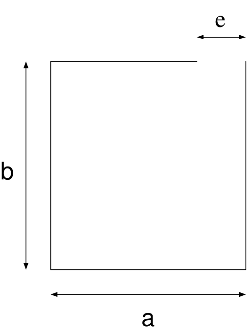
Figure 2: Rectangle of sizes $a$ and $b$ with a small absorbing segment of size $\varepsilon$ at the corner.

For example, the MFPT from a rectangle with sides $a$ and $b$ to an absorbing window of size $\varepsilon$ at the corner ($\alpha=\pi/2$, see Figure 2), is

$$E\tau=\frac{2|\Omega|}{\pi}\left[\log\frac{a}{\varepsilon}+\log\frac{2}{\pi}+\frac{\pi}{6}\frac{b}{a}+2\beta^{2}+O\left(\frac{\varepsilon}{a},\beta^{4}\right)\right],$$

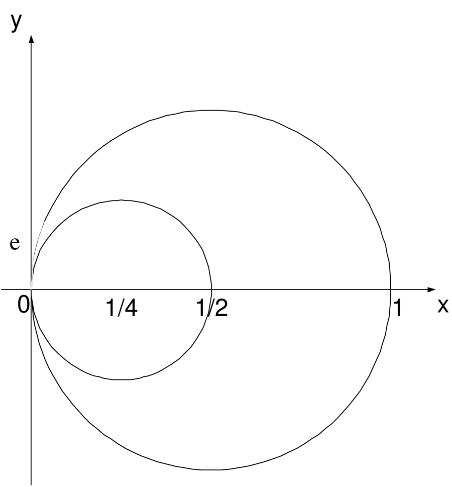
Figure 4: The point $(0,0)$ is a cusp point of the dotted domain bounded between the two circles. The small absorbing arc of length $\varepsilon$ is located at the cusp point.

where $|\Omega|=ab$ and $\beta=e^{-\pi b/a}$. The calculation of the second order term turns out to be similar to that in the annulus case. The pre-logarithmic factor $\displaystyle{\frac{|\Omega|_{g}}{D\alpha}}$ is the result of the different singularity of the Neumann function at the corner. It can be obtained by either the method of images, or by the conformal mapping $z\mapsto z^{\pi/\alpha}$ that flattens the corner. In the vicinity of a cusp $\alpha\to 0$, therefore the asymptotic expansion (1.3) is invalid. We find that near a cusp the MFPT grows algebraically fast as $\displaystyle{\frac{1}{\varepsilon^{\lambda}}}$, where $\lambda$ is the order of the cusp. Note that the MFPT grows faster to infinity as the boundary is more singular. The change of behavior from a logarithmic growth to an algebraic one expresses the fact that entering a cusp is a rare Brownian event. For example, the MFPT from the domain bounded between two tangent circles to a small arc at the common point (see Figure 4) is $E\tau=\displaystyle{\frac{|\Omega|}{(d^{-1}-1)D}}\left(\frac{1}{\varepsilon}+O(1)\right)$, where $d<1$ is the ratio of the radii. This result is obtained by mapping the cusped domain conformally onto the upper half plane. The singularity of the Neumann function is transformed as well. The leading order term of the asymptotics can be found for any domain that can be mapped conformally to the upper half plane.

In three dimensions the class of isolated singularities of the boundary is much richer than in the plane. The results of [4] cannot be generalized in a straightforward way to windows located near a singular point or arc of the boundary. We postpone the investigation of the MFPT to windows at isolated singular points in three dimensions to a future paper.

As a possible application of the present results, we mention the calculation of the diffusion coefficient from the statistics of the lifetime of a receptor in a corral on the surface of a neuronal spine [3].

2 Asymptotic approximation to the MFPT on a Riemannian manifold

We denote by $\mbox{\boldmath$x$}(t)$ the trajectory of a Brownian motion in a bounded domain $\Omega$ on a two-dimensional Riemannian manifold $(\Sigma,g)$. For a domain $\Omega\subset\Sigma$ with a smooth boundary $\partial\Omega$ (at least $C^{1}$), we denote by $|\Omega|_{g}$ the Riemannian surface area of $\Omega$ and by $|\partial\Omega|_{g}$ the arclength of its boundary, computed with respect to the metric $g$. The boundary $\partial\Omega$ is partitioned into an absorbing arc $\partial\Omega_{a}$ and the remaining part $\partial\Omega-\partial\Omega_{a}$ is reflecting for the Brownian trajectories. We assume that the absorbing part is small, that is,

$$\varepsilon=\frac{|\partial\Omega_{a}|_{g}}{|\partial\Omega|_{g}}\ll 1,$$

however, $\Sigma$ and $\Omega$ are independent of $\varepsilon$; only the partition of the boundary $\partial\Omega$ into absorbing and reflecting parts varies with $\varepsilon$.

The first passage time $\tau$ of the Brownian motion from $\Omega$ to $\partial\Omega_{a}$ has a finite mean and we define

$$u(\mbox{\boldmath$x$})=E[\tau\,|\,\mbox{\boldmath$x$}(0)=\mbox{\boldmath$x$}].$$

The function $u(\mbox{\boldmath$x$})$ satisfies the mixed Neumann-Dirichlet boundary value problem (see for example [6], [7])

$$D\Delta_{g}u(\mbox{\boldmath$x$}) = -1\quad\mbox{for}\quad\mbox{\boldmath$x$}\in\Omega$$ (2.1)

$$\frac{\partial u(\mbox{\boldmath$x$})}{\partial n} = 0\quad\mbox{for}\quad\mbox{\boldmath$x$}\in\partial\Omega-\partial\Omega_{a}$$ (2.2)

$$u(\mbox{\boldmath$x$}) = 0\quad\mbox{for}\quad\mbox{\boldmath$x$}\in\partial\Omega_{a},$$ (2.3)

where $\Delta_{g}$ is the Laplace-Beltrami operator on $\Sigma$ and $D$ is the diffusion coefficient. Obviously, $u(\mbox{\boldmath$x$})\to\infty$ as $\varepsilon\to 0$, except for $x$ in a boundary layer near $\partial\Omega_{a}$.

2.1 Expression of the MFPT using the Neumann function

We consider the Neumann function defined on $\Sigma$ by

$$\Delta_{g}N(\mbox{\boldmath$x$},\mbox{\boldmath$y$}) = -\delta(\mbox{\boldmath$x$}-\mbox{\boldmath$y$})+\frac{1}{|\Omega|_{g}},\quad\mbox{for}\quad\mbox{\boldmath$x$},\mbox{\boldmath$y$}\in\Omega$$ (2.4)

$$\frac{\partial N(\mbox{\boldmath$x$},\mbox{\boldmath$y$})}{\partial\mbox{\boldmath$n$}} = 0,\quad\mbox{for}\quad\mbox{\boldmath$x$}\in\partial\Omega,\ \mbox{\boldmath$y$}\in\Omega.$$

The Neumann function $N(\mbox{\boldmath$x$},\mbox{\boldmath$y$})$ is defined up to an additive constant and is symmetric [8]. The Neumann function exists for the domain $\Omega$, because the compatibility condition is satisfied (i.e., both sides of eq.(2.4) integrate to 0 over $\Omega$ due to the boundary condition). The Neumann function $N(\mbox{\boldmath$x$},\mbox{\boldmath$y$})$ is constructed by using a parametrix $H(\mbox{\boldmath$x$},\mbox{\boldmath$y$})$ [9] ,

$$H(\mbox{\boldmath$x$},\mbox{\boldmath$y$})=-\frac{h(d(\mbox{\boldmath$x$},\mbox{\boldmath$y$}))}{2\pi}\log d(\mbox{\boldmath$x$},\mbox{\boldmath$y$}),$$ (2.5)

where $d(\mbox{\boldmath$x$},\mbox{\boldmath$y$})$ is the Riemannian distance between $x$ and $y$ and $h(\cdot)$ is a regular function with compact support, equal to 1 in a neighborhood of $y$. As a consequence of the construction $N(\mbox{\boldmath$x$},\mbox{\boldmath$y$})-H(\mbox{\boldmath$x$},\mbox{\boldmath$y$})$ is a regular function on $\Omega$.

To derive an integral representation of the solution $u$, we multiply eq.(2.1) by $N(\mbox{\boldmath$x$},\mbox{\boldmath$y$})$, eq.(2.4) by $u(\mbox{\boldmath$x$})$, integrate with respect to $x$ over $\Omega$, and use Green’s formula to obtain the identity

$$\oint_{\partial\Omega}N(\mbox{\boldmath$x$}(\mbox{\boldmath$S$}),\mbox{\boldmath$\xi$})\frac{\partial u(\mbox{\boldmath$x$}(\mbox{\boldmath$S$}))}{\partial n}\,dS_{g} = -\frac{1}{|\Omega|_{g}}\int_{\Omega}u(\mbox{\boldmath$x$})\,dV_{g}+u(\mbox{\boldmath$\xi$})$$ (2.6)

$$-\int_{\Omega}N(\mbox{\boldmath$x$},\mbox{\boldmath$\xi$})\,dV_{g}.$$

The integral

$$C_{\varepsilon}=\displaystyle{\frac{1}{|\Omega|_{g}}\int_{\Omega}u(\mbox{\boldmath$x$})\,dV_{g}}$$ (2.7)

is an additive constant and the flux on the reflecting boundary vanishes, so we rewrite eq.(2.6) as

$$u(\mbox{\boldmath$\xi$})=C_{\varepsilon}+\int_{\Omega}N(\mbox{\boldmath$x$},\mbox{\boldmath$\xi$})\,dV_{g}+\int_{\partial\Omega_{a}}N(\mbox{\boldmath$x$}(\mbox{\boldmath$S$}),\mbox{\boldmath$\xi$})\frac{\partial u(\mbox{\boldmath$x$}(\mbox{\boldmath$S$}))}{\partial n}\,dS_{g},$$ (2.8)

where $S$ is the coordinate of a point on $\partial\Omega_{a}$, and $dS_{g}$ is arclength element on $\partial\Omega_{a}$ associated with the metric $g$. Setting

$$f(\mbox{\boldmath$S$})=\frac{\partial u(\mbox{\boldmath$x$}(\mbox{\boldmath$S$}))}{\partial n},$$

and choosing $\mbox{\boldmath$\xi$}\in\partial\Omega_{a}$ in eq.(2.8), we obtain

$$0=C_{\varepsilon}+\int_{\Omega}N(\mbox{\boldmath$x$},\mbox{\boldmath$\xi$})\,dV_{g}+\int_{\partial\Omega_{a}}N(\mbox{\boldmath$x$}(\mbox{\boldmath$S$}),\mbox{\boldmath$\xi$})f(\mbox{\boldmath$S$})\,dS_{g}.$$ (2.9)

The first integral in eq.(2.8) is a constant (independent of $\varepsilon$), because due to the symmetry of $N(\mbox{\boldmath$x$},\mbox{\boldmath$y$})$ eq.(2.4) gives the boundary value problem

$$\Delta_{\mbox{\boldmath$\xi$}}\int_{\Omega}N(\mbox{\boldmath$x$},\mbox{\boldmath$\xi$})\,dV_{g} = 0\quad\mbox{for}\quad\mbox{\boldmath$\xi$}\in\Omega$$

$$\frac{\partial}{\partial n(\mbox{\boldmath$\xi$})}\int_{\Omega}N(\mbox{\boldmath$x$},\mbox{\boldmath$\xi$})\,dV_{g} = 0\quad\mbox{for}\quad\mbox{\boldmath$\xi$}\in\partial\Omega,$$

whose solution is any constant. Changing the definition of the constant $C_{\varepsilon}$, equation (2.8) can be written as,

$$u(\mbox{\boldmath$\xi$})=\int_{\partial\Omega_{a}}N(\mbox{\boldmath$x$}(\mbox{\boldmath$S$}),\mbox{\boldmath$\xi$})f(\mbox{\boldmath$S$})\,dS_{g}+C_{\varepsilon},$$ (2.10)

and both $f(\mbox{\boldmath$S$})$ and $C_{\varepsilon}$ are determined by the absorbing condition (2.3)

$$0=\int_{\partial\Omega_{a}}N(\mbox{\boldmath$x$}(\mbox{\boldmath$S$}),\mbox{\boldmath$\xi$})f(\mbox{\boldmath$S$})\,dS_{g}+C_{\varepsilon}\quad\mbox{for}\quad\mbox{\boldmath$\xi$}\in\partial\Omega_{a}.$$ (2.11)

Equation (2.11) has been considered in [2] for a domain $\Sigma\subset\hbox{\bb R}^{2}$ as an integral equation for $f(\mbox{\boldmath$S$})$ and $C_{\varepsilon}$.

Actually, the boundary coordinate $S$ can be chosen as arclength on $\partial\Omega_{a}$, denoted $s$. Under the regularity assumptions of the boundary, the normal derivative $f(s)$ is a regular function, but develops a singularity as $\mbox{\boldmath$\xi$}(s)$ approaches the corner boundary of $\partial\Omega_{a}$ in $\partial\Omega$ [10]. Both can be determined from the representation (2.10), if all functions in eq.(2.11) and the boundary are analytic. In that case the solution has a series expansion in powers of arclength on $\Omega_{a}$. The method to compute $C_{\varepsilon}$ follows the same step as in [2].

2.2 Leading order asymptotics

Under our assumptions, $u(\mbox{\boldmath$\xi$})\to\infty$ as $\varepsilon\to 0$ for any fixed $\mbox{\boldmath$\xi$}\in\Omega$, so that eq.(2.7) implies that $C_{\varepsilon}\to\infty$ as well. It follows from eq.(2.11) that the integral in (2.11) decreases to $-\infty$.

An origin $0\in\partial\Omega_{a}$ is fixed and the boundary $\partial\Omega$ is parameterized by $(x(s),y(s))$. We rescale $s$ so that $\partial\Omega=\left\{(x(s),y(s))\,:\,-\frac{1}{2}<s\leq\frac{1}{2}\right\}$ and $\left(x\left(-\frac{1}{2}\right),y\left(-\frac{1}{2}\right)\right)=\left(x\left(\frac{1}{2}\right),y\left(\frac{1}{2}\right)\right)$. We assume that the functions $x(s)$ and $y(s)$ are real analytic in the interval $2|s|<1$ and that the absorbing part of the boundary $\partial\Omega_{a}$ is the arc

$$\partial\Omega_{a}=\left\{(x(s),y(s))\,:\,|s|<\varepsilon\right\}.$$

The Neumann function can be written as

$$N(\mbox{\boldmath$x$},\mbox{\boldmath$\xi$})=-\frac{1}{2\pi}\log d(\mbox{\boldmath$x$},\mbox{\boldmath$\xi$})+v_{N}(\mbox{\boldmath$x$},\mbox{\boldmath$\xi$}),\quad\hbox{for}\quad\mbox{\boldmath$x$}\in B_{\delta}(\mbox{\boldmath$\xi$}),$$ (2.12)

where $B_{\delta}(\mbox{\boldmath$\xi$})$ is a geodesic ball of radius $\delta$ centered at $\xi$ and $v_{N}(\mbox{\boldmath$x$};\mbox{\boldmath$\xi$})$ is a regular function. We consider a normal geodesic coordinate system $(x,y)$ at the origin, such that one of the coordinates coincides with the tangent coordinate to $\partial\Omega_{a}$. We choose unit vectors $\mbox{\boldmath$e$}_{1},\mbox{\boldmath$e$}_{2}$ as an orthogonal basis in the tangent plane at 0 so that for any vector field $\mbox{\boldmath$X$}=x_{1}\mbox{\boldmath$e$}_{1}+x_{2}\mbox{\boldmath$e$}_{2}$, the metric tensor $g$ can be written as

$$g_{ij}=\delta_{ij}+\varepsilon^{2}\sum_{kl}a^{kl}_{ij}x_{k}x_{l}+o(\varepsilon^{2}),$$ (2.13)

where $|x_{k}|\leq 1$, because $\varepsilon$ is small. It follows that for $\mbox{\boldmath$x$},\mbox{\boldmath$y$}$ inside the geodesic ball or radius $\varepsilon$, centered at the origin, $d(\mbox{\boldmath$x$},\mbox{\boldmath$y$})=d_{E}(\mbox{\boldmath$x$},\mbox{\boldmath$y$})+O(\varepsilon^{2})$, where $d_{E}$ is the Euclidean metric. We can now use the computation given in the Euclidean case in [2]. To estimate the solution of equation (2.11), we recall that when both $x$ and $\xi$ are on the boundary, $v_{N}(\mbox{\boldmath$x$},\mbox{\boldmath$\xi$})$ becomes singular (see [8, p.247, eq.(7.46)]) and the singular part gains a factor of 2, due to the singularity of the “image charge”. Denoting by $\tilde{v}_{N}$ the new regular part, equation (2.11) becomes

$$\int_{|s^{\prime}|<\varepsilon}\left[\tilde{v}_{N}(\mbox{\boldmath$x$}(s^{\prime});\mbox{\boldmath$\xi$}(s))-\frac{\log d(\mbox{\boldmath$x$}(s),\mbox{\boldmath$\xi$}(s^{\prime}))}{\pi}\right]f(s^{\prime})\,S(ds^{\prime})=C_{\varepsilon},$$ (2.14)

where $S(ds^{\prime})$ is the induced measure element on the boundary, and $\mbox{\boldmath$x$}=(x(s),y(s))$, $\mbox{\boldmath$\xi$}=(\xi(s),\eta(s))$. Now, we expand the integral in eq.(2.14), as in [2],

$$\log d(\mbox{\boldmath$x$}(s),\mbox{\boldmath$\xi$}(s^{\prime}))=\log\left(\sqrt{(x(s^{\prime})-\xi(s))^{2}+(y(s^{\prime})-\eta(s))^{2}}\,\left(1+O(\varepsilon^{2})\right)\right)$$

and

$$S(ds)f(s)=\sum_{j=0}^{\infty}f_{j}s^{j}\,ds,\quad\tilde{v}_{N}(\mbox{\boldmath$x$}(s^{\prime});\mbox{\boldmath$\xi$}(s))S(ds^{\prime})=\sum_{j=0}^{\infty}v_{j}(s^{\prime})s^{j}\,ds^{\prime}$$ (2.15)

for $|s|<\varepsilon$, where $v_{j}(s^{\prime})$ are known coefficients and $f_{j}$ are unknown coefficients, to be determined from eq.(2.14). To expand the logarithmic term in the last integral in eq.(2.14), we recall that $x(s^{\prime}),y(s^{\prime}),\xi(s)$, and $\eta(s)$ are analytic functions of their arguments in the intervals $|s|<\varepsilon$ and $|s^{\prime}|<\varepsilon$, respectively. Therefore

$$\int_{-\varepsilon}^{\varepsilon}(s^{\prime})^{n}\log d(\mbox{\boldmath$x$}(s),\mbox{\boldmath$\xi$}(s^{\prime}))\,ds^{\prime}=$$ (2.16)

$$\int_{-\varepsilon}^{\varepsilon}(s^{\prime})^{n}\log\sqrt{(x(s^{\prime})-\xi(s))^{2}+(y(s^{\prime})-\eta(s))^{2}}\left(1+O(\varepsilon^{2})\right)\,ds^{\prime}=$$

$$\int_{-\varepsilon}^{\varepsilon}(s^{\prime})^{n}\log\left\{|s^{\prime}-s|\left(1+O\left((s^{\prime}-s)^{2}\right)\right)\right\}\left(1+O(\varepsilon^{2})\right)\,ds^{\prime}.$$

We keep in Taylor’s expansion of $\log\left\{|s^{\prime}-s|\left(1+O\left((s^{\prime}-s)^{2}\right)\right)\right\}$ only the leading term, because higher order terms contribute positive powers of $\varepsilon$ to the series

$$\int_{-\varepsilon}^{\varepsilon}\log(s-s^{\prime})^{2}\,ds^{\prime}=4\varepsilon\left(\log\varepsilon-1\right)+2\sum_{j=1}^{\infty}\frac{1}{(2j-1)j}\frac{s^{2j}}{\varepsilon^{2j-1}}.$$ (2.17)

For even $n\geq 0$, we have

$$\int_{-\varepsilon}^{\varepsilon}(s^{\prime})^{n}\log(s-s^{\prime})^{2}\,ds^{\prime}=$$

$$4\left(\frac{\varepsilon^{n+1}}{n+1}\log\varepsilon-\frac{\varepsilon^{n+1}}{(n+1)^{2}}\right)-2\sum_{j=1}^{\infty}s^{2j}\frac{\varepsilon^{n-2j+1}}{j(n-2j+1)},$$ (2.18)

whereas for odd $n$, we have

$$\int_{-\varepsilon}^{\varepsilon}(s^{\prime})^{n}\log(s-s^{\prime})^{2}\,ds^{\prime}=-4\sum_{j=1}^{\infty}\frac{s^{2j+1}}{2j+1}\frac{\varepsilon^{n-2j}}{n-2j}.$$ (2.19)

Using the above expansion, we rewrite eq.(2.14) as

$$0 = \int_{-\varepsilon}^{\varepsilon}\left\{\frac{-1}{\pi}\log\left[|s^{\prime}-s|^{2}\left(1+O\left((s^{\prime}-s)^{2}\right)\right)(1+O(\varepsilon^{2}))\right]+\sum_{j=0}^{\infty}v_{j}(s^{\prime})s^{j}\right\}\times$$

$$\sum_{j=0}^{\infty}f_{j}s^{\prime j}\,ds^{\prime}+C_{\varepsilon},$$

and expand in powers of $s$. At the leading order, we obtain

$$\varepsilon\left(\log\varepsilon-1\right)f_{0}+\sum_{p}\left(\frac{\varepsilon^{2p+1}}{2p+1}\log\varepsilon-\frac{\varepsilon^{2p+1}}{(2p+1)^{2}}\right)f_{2p}=$$

$$\frac{\pi}{2}\int_{-\varepsilon}^{\varepsilon}v_{0}(s^{\prime})\,ds^{\prime}+C_{\varepsilon}.$$ (2.20)

Equation (2.20) and

$$\frac{1}{2}\int_{-\varepsilon}^{\varepsilon}f(s)\,S(ds)=\sum_{p}\frac{\varepsilon^{2p+1}}{(2p+1)}f_{2p}$$

determine the leading order term in the expansion of $C_{\varepsilon}$. Indeed, integrating eq.(2.1) over the domain $\Omega$, we see that the compatibility condition gives

$$\int_{-\varepsilon}^{\varepsilon}f(s)\,S(ds)=-|\Omega|_{g},$$ (2.21)

and using the fact that $\displaystyle{\int}_{-\varepsilon}^{\varepsilon}v_{0}(s^{\prime})S(ds^{\prime})=O(\varepsilon)$, we find that the leading order expansion of $C_{\varepsilon}$ in eq.(2.20) is

$$C_{\varepsilon}=\frac{|\Omega|_{g}}{\pi}\left[\log\frac{1}{\varepsilon}+O(1)\right]\quad\mbox{for $\varepsilon\ll 1$.}$$ (2.22)

If the diffusion coefficient is $D$, eq.(2.10) gives the MFPT from a point $\mbox{\boldmath$x$}\in\Omega$, outside the boundary layer, as

$$E[\tau\,|\,\mbox{\boldmath$x$}]=u(\mbox{\boldmath$x$})=\frac{|\Omega|_{g}}{\pi D}\left[\log\frac{1}{\varepsilon}+O(1)\right]\quad\mbox{for $\varepsilon\ll 1$.}$$ (2.23)

3 The annulus problem

We consider a Brownian particle that is confined in the annulus $R_{1}<r<R_{2}$. The particle can exit the annulus through a narrow opening of the inner circle (see Fig.1). The MFPT $v(\mbox{\boldmath$x$})$ satisfies

$$\Delta v = -1,\quad\mbox{for}\quad R_{1}<r<R_{2},$$ (3.1)

$$\frac{\partial v}{\partial r} = 0,\quad\mbox{for}\quad r=R_{2},$$

$$\frac{\partial v}{\partial r} = 0,\quad\mbox{for}\quad r=R_{1},\;|\theta-\pi|>\varepsilon,$$

$$v = 0,\quad\mbox{for}\quad r=R_{1},\;|\theta-\pi|<\varepsilon.$$

The function $w=\displaystyle{\frac{R_{1}^{2}-r^{2}}{4}}$ is a solution of the Dirichlet problem for eq.(3.1) in the exterior domain of the inner circle $r>R_{1}$. More specifically, it satisfies the boundary value problem

$$\Delta w = -1,\quad\mbox{for}\quad R_{1}<r<R_{2},$$

$$\frac{\partial w}{\partial r} = -\frac{1}{2}R_{1},\quad\mbox{for}\quad r=R_{1},$$

$$\frac{\partial w}{\partial r} = -\frac{1}{2}R_{2},\quad\mbox{for}\quad r=R_{2},$$

$$w = 0,\quad\mbox{for}\quad r=R_{1}.$$ (3.2)

The function $u=v-w$ satisfies

$$\Delta u = 0,\quad\mbox{for}\quad R_{1}<r<R_{2},$$

$$\frac{\partial u}{\partial r} = \frac{1}{2}R_{2},\quad\mbox{for}\quad r=R_{2},$$

$$\frac{\partial u}{\partial r} = \frac{1}{2}R_{1},\quad\mbox{for}\quad r=R_{1},\;|\theta-\pi|>\varepsilon,$$

$$u = 0,\quad\mbox{for}\quad r=R_{1},\;|\theta-\pi|<\varepsilon.$$ (3.3)

Separation of variables produces the solution

$$u(r,\theta)=\frac{a_{0}}{2}+\sum_{n=1}^{\infty}\left[a_{n}\left(\frac{r}{R_{2}}\right)^{n}+b_{n}\left(\frac{R_{2}}{r}\right)^{n}\right]\cos n\theta+\alpha\log\left(\frac{r}{R_{1}}\right),$$ (3.4)

where $a_{n},\,b_{n}$ and $\alpha$ are to be determined by the boundary conditions. Differentiating with respect to $r$ yields

$$\frac{\partial u}{\partial r}=\sum_{n=1}^{\infty}n\left[\frac{a_{n}}{R_{2}}\left(\frac{r}{R_{2}}\right)^{n-1}-\frac{b_{n}R_{2}}{r^{2}}\left(\frac{R_{2}}{r}\right)^{n-1}\right]\cos n\theta+\frac{\alpha}{r}.$$ (3.5)

Setting $r=R_{2}$ gives

$$\frac{1}{2}R_{2}=\frac{1}{R_{2}}\left[\sum_{n=1}^{\infty}n\left(a_{n}-b_{n}\right)\cos n\theta+\alpha\right],$$ (3.6)

therefore, $a_{n}=b_{n}$ and $\alpha=\displaystyle{\frac{1}{2}}R_{2}^{2}$, and we have

$$u(r,\theta)=\frac{a_{0}}{2}+\sum_{n=1}^{\infty}a_{n}\left[\left(\frac{r}{R_{2}}\right)^{n}+\left(\frac{R_{2}}{r}\right)^{n}\right]\cos n\theta+\frac{1}{2}R_{2}^{2}\log\left(\frac{r}{R_{1}}\right).$$ (3.7)

The boundary conditions at $r=R_{1}$ become the dual series equations

$$\frac{a_{0}}{2}+\sum_{n=1}^{\infty}a_{n}\left[\left(\frac{R_{2}}{R_{1}}\right)^{n}+\left(\frac{R_{1}}{R_{2}}\right)^{n}\right]\cos n\theta = 0,\quad\mbox{for}\quad|\theta-\pi|<\varepsilon,$$

$$\sum_{n=1}^{\infty}na_{n}\left[\left(\frac{R_{2}}{R_{1}}\right)^{n+1}-\left(\frac{R_{1}}{R_{2}}\right)^{n-1}\right]\cos n\theta = \frac{R_{2}}{2R_{1}}\left(R_{2}^{2}-R_{1}^{2}\right),\quad\mbox{for}\quad|\theta-\pi|>\varepsilon.$$

Setting

$$c_{n}=\frac{R_{1}}{R_{2}}\left[\left(\frac{R_{2}}{R_{1}}\right)^{n+1}-\left(\frac{R_{1}}{R_{2}}\right)^{n-1}\right]a_{n},\quad\mbox{for }\quad n\geq 1,$$ (3.8)

and $c_{0}=a_{0}$ converts the dual series equations to

$$\frac{c_{0}}{2}+\sum_{n=1}^{\infty}\frac{c_{n}}{1+H_{n}}\cos n\theta = 0,\quad\mbox{for}\quad\pi-\varepsilon<\theta<\pi,$$ (3.9)

$$\sum_{n=1}^{\infty}nc_{n}\cos n\theta = \frac{1}{2}(R_{2}^{2}-R_{1}^{2}),\quad\mbox{for}\quad 0<\theta<\pi-\varepsilon,$$ (3.10)

where $H_{n}=\displaystyle{-}\frac{2\beta^{2n}}{1+\beta^{2n}}$ for $n\geq 1$, and $H_{0}=0$, with $\beta=\displaystyle{\frac{R_{1}}{R_{2}}}<1$. Note that $H_{n}=O(\beta^{2n})$ which tends to zero exponentially fast (much faster than the $n^{-1}$ decay required for the Collins method [14, 15], see also [4]).

The case $H_{n}\equiv 0$ was solved in [5]. We now try to find the correction of that result due to the non vanishing $H_{n}$. As in [5] the equation

$$\frac{c_{0}}{2}+\sum_{n=1}^{\infty}\frac{c_{n}}{1+H_{n}}\cos n\theta=$$

$$\cos\frac{\theta}{2}\int_{\theta}^{\pi-\varepsilon}\frac{h_{1}(t)\,dt}{\sqrt{\cos\theta-\cos t}}\quad\mbox{for}\quad\mbox{for}\quad 0<\theta<\pi-\varepsilon$$

defines the function $h_{1}(\theta)$ uniquely for $0<\theta<\pi-\varepsilon$, the coefficients are given by

$$c_{n}=\frac{1+H_{n}}{\sqrt{2}}\int_{0}^{\pi-\varepsilon}h_{1}(t)\left[P_{n}(\cos t)+P_{n-1}(\cos t)\right]\,dt,$$ (3.11)

and

$$c_{0}=\sqrt{2}\int_{0}^{\pi-\varepsilon}h_{1}(t)\,dt.$$ (3.12)

Integrating equation (3.10) gives

$$\sum_{n=1}^{\infty}c_{n}\sin n\theta=\frac{1}{2}\left(R_{2}^{2}-R_{1}^{2}\right)\theta,\quad\mbox{for}\quad 0<\theta<\pi-\varepsilon.$$ (3.13)

Substituting eq.(3.13) in equation (3.11), changing the order of summation and integration, while using [11, eq.(2.6.31)],

$$\frac{1}{\sqrt{2}}\sum_{n=1}^{\infty}[P_{n}(\cos t)+P_{n-1}(\cos t)]\sin n\theta=\frac{\cos\frac{1}{2}\theta H(\theta-t)}{\sqrt{\cos t-\cos\theta}},$$ (3.14)

we obtain for $0<\theta<\pi-\varepsilon,$

$$\int_{0}^{\theta}\frac{h_{1}(t)}{\sqrt{\cos t-\cos\theta}}\,dt+\int_{0}^{\pi-\varepsilon}K_{\beta}(\theta,t)h_{1}(t)\,dt=\frac{\left(R_{2}^{2}-R_{1}^{2}\right)\theta}{2\cos\displaystyle{\frac{\theta}{2}}},$$ (3.15)

where the kernel $K_{\beta}$ is

$$K_{\beta}(\theta,t) = \frac{1}{\sqrt{2}\cos\displaystyle{\frac{\theta}{2}}}\sum_{n=1}^{\infty}H_{n}\left(P_{n}(\cos t)+P_{n-1}(\cos t)\right)\sin n\theta$$ (3.16)

$$= -2\sqrt{2}(1+\cos t)\sin\frac{\theta}{2}\,\beta^{2}+O(\beta^{4}).$$

The infinite sum in eq.(3.16) is approximated by its first term, while using the first two Legendre polynomials $P_{0}(x)=1,\;P_{1}(x)=x$. Using Abel’s inversion formula applied to equation (3.15), we find that

$$h_{1}(t)-\int_{0}^{\pi-\varepsilon}\tilde{K}_{\beta}(t,s)h_{1}(s)\,ds=\frac{R_{2}^{2}-R_{1}^{2}}{\pi}\frac{d}{dt}\int_{0}^{t}\frac{u\sin\displaystyle{\frac{u}{2}}}{\sqrt{\cos u-\cos t}}\,du,$$ (3.17)

where the kernel $\tilde{K}_{\beta}$ is

$$\tilde{K}_{\beta}(t,s) = -\frac{1}{\pi}\frac{d}{dt}\int_{0}^{t}\frac{K_{\beta}(u,s)\sin u}{\sqrt{\cos u-\cos t}}\,du$$

$$= \beta^{2}\,\frac{2\sqrt{2}(1+\cos s)}{\pi}\frac{d}{dt}\int_{0}^{t}\frac{\sin\displaystyle{\frac{u}{2}}\,\sin u}{\sqrt{\cos u-\cos t}}\,du+O(\beta^{4}).$$

The substitution

$$s=\sqrt{\frac{\cos u-\cos t}{2}}$$ (3.19)

gives

$$\int_{0}^{t}\frac{\sin\displaystyle{\frac{u}{2}}\,\sin u}{\sqrt{\cos u-\cos t}}\,du=\frac{\pi}{\sqrt{2}}\sin^{2}\frac{t}{2},$$ (3.20)

therefore,

$$\tilde{K}_{\beta}(t,s)=2\beta^{2}\cos^{2}\frac{s}{2}\sin t+O(\beta^{4}).$$ (3.21)

Equation (3.17) is a Fredholm integral equation of the second kind for $h_{1}$, of the form

$$(I-\tilde{K}_{\beta})h=z,$$ (3.22)

where

$$z(t)=\displaystyle{\frac{R_{2}^{2}-R_{1}^{2}}{\pi}\frac{d}{dt}\int_{0}^{t}\frac{u\sin\displaystyle{\frac{u}{2}}}{\sqrt{\cos u-\cos t}}}\,du.$$

Therefore, we $h$ can be expanded as

$$h=z+\tilde{K}_{\beta}z+\tilde{K}_{\beta}^{2}z+\ldots,$$ (3.23)

which converges in $L^{2}$. Since $c_{0}=\sqrt{2}\langle h,1\rangle$ (eq.(3.12)), we find an asymptotic expansion of the form

$$c_{0}=\sqrt{2}\left[\langle z,1\rangle+\langle\tilde{K}_{\beta}z,1\rangle+\ldots\right].$$ (3.24)

The leading order term of this expansion was calculated in [5]. We now estimate the error term $\langle\tilde{K}_{\beta}z,1\rangle$, which is also the $O(\beta^{2})$ correction. Integrating by parts and changing the order of integration yields

$$\tilde{K}_{\beta}z(t) = 2\beta^{2}\frac{R_{2}^{2}-R_{1}^{2}}{\pi}\sin t\int_{0}^{\pi}\cos^{2}\frac{s}{2}\,ds\,\frac{d}{ds}\int_{0}^{s}\frac{u\sin\displaystyle{\frac{u}{2}}}{\sqrt{\cos u-\cos s}}\,du$$ (3.25)

$$= \beta^{2}\frac{R_{2}^{2}-R_{1}^{2}}{\pi}\sin t\int_{0}^{\pi}\sin s\,ds\int_{0}^{s}\frac{u\sin\displaystyle{\frac{u}{2}}\,du}{\sqrt{\cos u-\cos s}}$$

$$= \sqrt{2}\beta^{2}(R_{2}^{2}-R_{1}^{2})\sin t.$$

Therefore,

$$\langle\tilde{K}_{\beta}z,1\rangle=\sqrt{2}\beta^{2}(R_{2}^{2}-R_{1}^{2})\int_{0}^{\pi}\sin t\,dt=2\sqrt{2}\beta^{2}(R_{2}^{2}-R_{1}^{2}).$$ (3.26)

We conclude that

$$c_{0}=(R_{2}^{2}-R_{1}^{2})\left[2\log\frac{1}{\varepsilon}+2\log 2+4\beta^{2}+O(\varepsilon,\beta^{4})\right].$$ (3.27)

The MFPT averaged with respect to a uniform initial distribution is

$$E\tau = \frac{c_{0}}{2}+\frac{1}{2}\frac{R_{2}^{4}}{R_{2}^{2}-R_{1}^{2}}\log\frac{R_{2}}{R_{1}}-\frac{1}{4}R_{2}^{2}$$

$$= (R_{2}^{2}-R_{1}^{2})\left[\log\frac{1}{\varepsilon}+\log 2+2\beta^{2}\right]+\frac{1}{2}\frac{R_{2}^{2}}{1-\beta^{2}}\log\frac{1}{\beta}-\frac{1}{4}R_{2}^{2}+O(\varepsilon,\beta^{4})R_{2}^{2}.$$

Note that there are two different logarithmic contributions to the MFPT. The “narrow escape” small parameter $\varepsilon$ contributes

$$\frac{|\Omega|_{g}}{\pi}\log\frac{1}{\varepsilon},$$ (3.29)

as expected from the general theory (equation (1.1)), whereas the parameter $\beta$ contributes

$$\frac{|\Omega|_{g}}{2\pi}\log\frac{1}{\beta}.$$ (3.30)

These asymptotics differ by a factor 2, because they account for different singular behaviors. The asymptotic expansion (3.29) comes out from a singular perturbation problem with singular flux near the edges, boundary layer and an outer solution, whereas the asymptotics (3.30) is an immediate result of the singularity of the Neumann function, with a regular flux.

The exit problem in an annulus with the absorbing window located at the outer circle is solved by applying the complex inversion mapping $z\to 1/z$, which maps the annulus into itself and replaces the roles of the inner and outer circles. In such case, in the limit $\beta\to 0$, the circular disk problem is recovered, where it was shown that the maximum exit time is attained at the antipode point on the outer circle. Since the inversion mapping exchanges the inner and outer circles, we conclude that for the original annulus problem, where the absorbing boundary is located at the inner circle, the maximal exit time is attained at the inner circle, at the antipode of the center of the hole. This point is close by to the hole itself, a result which is somewhat counterintuitive. Note that (3) is valid, with the obvious modifications, for any domain that is conformally equivalent to the annulus.

4 Domains with corners

Consider a Brownian motion in a rectangle $\Omega=(0,a)\times(0,b)$ of area $ab$. The boundary is reflecting except the small absorbing segment $\partial\Omega_{a}=[a-\varepsilon,a]\times\{b\}$ (see Fig. 2). The MFPT $v(x,y)$ satisfies the boundary value problem

$$\Delta v = -1,\quad(x,y)\in\Omega,$$

$$v = 0,\quad(x,y)\in\partial\Omega_{a},$$

$$\frac{\partial v}{\partial n} = 0,\quad(x,y)\in\partial\Omega-\partial\Omega_{a}.$$ (4.1)

The function $f=\displaystyle{\frac{b^{2}-y^{2}}{2}}$ satisfies

$$\Delta f = -1,\quad(x,y)\in\Omega,$$

$$f = 0,\quad(x,y)\in\partial\Omega_{a},$$

$$\frac{\partial f}{\partial n} = 0,\quad(x,y)\in\{0\}\times[0,b]\cup\{a\}\times[0,b]\cup[0,a]\times\{0\},$$

$$\frac{\partial f}{\partial n} = -b,\quad(x,y)\in[0,a-\varepsilon]\times\{b\},$$ (4.2)

therefore, the function $u=v-f$ satisfies

$$\Delta u = 0,\quad(x,y)\in\Omega,$$

$$u = 0,\quad(x,y)\in\partial\Omega_{a},$$

$$\frac{\partial u}{\partial n} = 0,\quad(x,y)\in\{0\}\times[0,b]\cup\{a\}\times[0,b]\cup[0,a]\times\{0\},$$

$$\frac{\partial u}{\partial n} = b,\quad(x,y)\in[0,a-\varepsilon]\times\{b\}.$$ (4.3)

A solution for $u$ in the form of separation of variables is

$$u(x,y)=\frac{a_{0}}{2}+\sum_{n=1}^{\infty}a_{n}\cosh\frac{\pi ny}{a}\cos\frac{\pi nx}{a},$$ (4.4)

where the coefficients $a_{n}$ are to be determined by the boundary conditions at $y=b$

$$u(x,b) = \frac{a_{0}}{2}+\sum_{n=1}^{\infty}a_{n}\cosh\frac{\pi nb}{a}\cos\frac{\pi nx}{a}=0,\quad x\in(a-\varepsilon,a),$$

$$\frac{\partial u}{\partial y}(x,b) = \frac{\pi}{a}\sum_{n=1}^{\infty}na_{n}\sinh\frac{\pi nb}{a}\cos\frac{\pi nx}{a}=b,\quad x\in(0,a-\varepsilon).$$ (4.5)

Setting $c_{n}=a_{n}\sinh\displaystyle{\frac{\pi nb}{a}}$, we have

$$\frac{c_{0}}{2}+\sum_{n=1}^{\infty}\frac{c_{n}}{1+H_{n}}\cos n\theta = 0,\quad\pi-\delta<\theta<\pi,$$

$$\sum_{n=1}^{\infty}nc_{n}\cos n\theta = \frac{ab}{\pi},\quad 0<\theta<\pi-\delta,$$ (4.6)

where $\delta=\displaystyle{\frac{\pi\varepsilon}{a}}$ and $H_{n}=\tanh\left(\displaystyle{\frac{\pi nb}{a}}\right)-1,n\geq 1$. Note that $H_{n}=O\left(\beta^{2n}\right)$ for $\beta=\exp\left\{-\displaystyle{\frac{\pi b}{a}}\right\}<1$. The rectangle problem and annulus problem (eq. (3.10)) are almost mathematically equivalent, and equation (3.27) gives the value of $c_{0}$

$$c_{0} = \frac{2ab}{\pi}\left[2\log\frac{1}{\delta}+2\log 2+4\beta^{2}+O(\delta,\beta^{4})\right]$$ (4.7)

$$= \frac{4ab}{\pi}\left[\log\frac{a}{\varepsilon}+\log\frac{2}{\pi}+2\beta^{2}+O\left(\frac{\varepsilon}{a},\beta^{4}\right)\right].$$

The error term due to $O(\beta^{4})$ is generally small. For example, in a square $a=b$ and $\beta=e^{-\pi}$ so that $\beta^{4}\approx 3\times 10^{-6}$. The MFPT averaged with respect to a uniform initial distribution is

$$E\tau=\frac{c_{0}}{2}+\frac{b^{2}}{3}=\frac{2ab}{\pi}\left[\log\frac{a}{\varepsilon}+\log\frac{2}{\pi}+\frac{\pi}{6}\frac{b}{a}+2\beta^{2}+O\left(\frac{\varepsilon}{a},\beta^{4}\right)\right].$$ (4.8)

The leading order term of the MFPT is

$$\frac{2|\Omega|}{\pi}\log\frac{a}{\varepsilon},$$ (4.9)

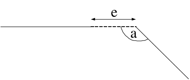
Figure 3: A small opening near a corner of angle $\alpha$.

which is twice as large than (3.29). The general result (1.1) was proved for a domain with smooth boundary (at least $C^{1}$). However, in the rectangle example, the small hole is located at the corner. The additional factor 2 is the result of the different singularity of the Neumann function at the corner, which is 4 times larger than that of the Green function. At the corner there are 3 image charges — the number of images that one sees when standing near two perpendicular mirror plates. In general, for a small hole located at a corner of an opening angle $\alpha$ (see Fig. 3), the MFPT is to leading order

$$E\tau=\frac{|\Omega|}{D\alpha}\left(\log\frac{1}{\varepsilon}+O(1)\right).$$ (4.10)

This result is a consequence of the method of images for integer values of $\displaystyle{\frac{\pi}{\alpha}}$. For non-integer $\displaystyle{\frac{\pi}{\alpha}}$ we use the complex mapping $z\mapsto z^{\pi/\alpha}$ that flattens the corner. The upper half plane Neumann function $\displaystyle{\frac{1}{\pi}}\log z$ is mapped to $\displaystyle{\frac{1}{\alpha}}\log z$ and the analysis of Section 2 gives (4.10).

To see that the area factor $|\Omega|$ remains unchanged under the conformal mapping $f:(x,y)\mapsto(u(x,y),v(x,y))$, we note that this factor is a consequence of the compatibility condition, that relates the area to the integral

$$\int_{\Omega}\Delta_{(x,y)}w\,dx\,dy=-\displaystyle{\frac{|\Omega|}{D}},$$

where $w(x,y)=E[\tau|\,x(0)=x,y(0)=y]$ satisfies $\Delta_{(x,y)}w=-1/D$. The Laplacian transforms according to

$$\Delta_{(x,y)}w=(u_{x}^{2}+u_{y}^{2})\Delta_{(u,v)}w,$$

by the Cauchy-Riemann equations and the Jacobian of the transformation is $J=u_{x}^{2}+u_{y}^{2}$. Therefore,

$$\int_{\Omega}\Delta_{(x,y)}w\,dx\,dy=\int_{f(\Omega)}\Delta_{(u,v)}w\,du\,dv.$$

This means that the compatibility condition of Section 2 remains unchanged and gives the area of the original domain.

5 Domains with cusps

Here we find the leading order term of the MFPT for small holes located near a cusp of the boundary. A cusp is a singular point of the boundary. As $\alpha=0$ at the cusp, one expects to find a different asymptotic expansion than (4.10). As an example, consider the Brownian motion inside the domain bounded between the circles $(x-1/2)^{2}+y^{2}=1/4$ and $(x-1/4)^{2}+y^{2}=1/16$ (see Figure 4). The conformal mapping $z\mapsto\exp\{\pi i(1/z-1)\}$ maps this domain onto the upper half plane. Therefore, the MFPT is to leading order

$$E\tau=\frac{|\Omega|}{D}\left(\frac{1}{\varepsilon}+O(1)\right).$$ (5.1)

This result can also be obtained by mapping the cusped domain to the unit circle. The absorbing boundary is then transformed to an exponentially small arc of length $\exp\{-\pi/\varepsilon\}+O(\exp\{-2\pi/\varepsilon\})$, and equation (5.1) is recovered.

If the ratio between the two radii is $d<1$, then the conformal map that maps the domain between the two circles to the upper half plane is $\exp\left\{\displaystyle{\frac{\pi i}{d^{-1}-1}}(1/z-1)\right\}$ (for $d=1/2$ we arrive at the previous example), so the MFPT is to leading order

$$E\tau=\frac{|\Omega|}{(d^{-1}-1)D}\left(\frac{1}{\varepsilon}+O(1)\right).$$ (5.2)

The MFPT tends algebraically fast to infinity, much faster than the $O\left(\log\displaystyle{\frac{1}{\varepsilon}}\right)$ behavior near smooth or corner boundaries. The MFPT for a cusp is much larger because it is more difficult for the Brownian motion to enter the cusp than to enter a corner. The MFPT (5.2) can be written in terms of $d$ instead of the area. Substituting $|\Omega|=\pi R^{2}(1-d^{2})$, we find

$$E\tau=\frac{\pi R^{2}d(1+d)}{D}\left(\frac{1}{\varepsilon}+O(1)\right),$$ (5.3)

where $R$ is the radius of the outer circle. Note that although the area of $\Omega$ is a monotonically decreasing function of $d$, the MFPT is a monotonically increasing function of $d$ and tends to a finite limit as $d\to 1$.

Similarly, one can consider different types of cusps and find that the leading order term for the MFPT is proportional to $1/\varepsilon^{\lambda}$, where $\lambda$ is a parameter that describes the order of the cusp, and can be obtained by the same technique of conformal mapping.

6 Diffusion on a 3-sphere

6.1 Small absorbing cap

Consider a Brownian motion on the surface of a 3-sphere of radius $R$ [16], described by the spherical coordinates $(\theta,\phi)$

$$x=R\sin\theta\cos\phi,\quad y=R\sin\theta\sin\phi,\quad z=R\cos\theta.$$

The particle is absorbed when it reaches a small spherical cap. We center the cap at the north pole, $\theta=0$. Furthermore, the FPT to hit the spherical cap is independent of the initial angle $\phi$, due to rotational symmetry. Let $v(\theta)$ be the MFPT to hit the spherical cap. Then $v$ satisfies

$$\Delta_{M}v=-1,$$ (6.1)

where $\Delta_{M}$ is the Laplace-Beltrami operator [16] of the 3-sphere. This Laplace-Beltrami operator $\Delta_{M}$ replaces the regular plane Laplacian, because the diffusion occurs on a manifold [16, and reference therein]. For a function $v$ independent of the angle $\phi$ the Laplace-Beltrami operator is (see Appendix A)

$$\Delta_{M}v=R^{-2}\left(v^{\prime\prime}+\cot\theta\,v^{\prime}\right).$$ (6.2)

The MFPT also satisfies the boundary conditions

$$v^{\prime}(\pi)=0,\quad v(\delta)=0,$$ (6.3)

where $\delta$ is the opening angle of the spherical cap. The solution of the boundary value problem (6.2), (6.3) is given by

$$v(\theta)=2R^{2}\log\frac{\sin(\theta/2)}{\sin(\delta/2)}.$$ (6.4)

Not surprisingly, the maximum of the MFPT is attained at the point $\theta=\pi$ with the value

$$v_{\mbox{max}}=v(\pi)=-2R^{2}\log\sin\displaystyle{\frac{\delta}{2}}=2R^{2}\left(\log\frac{1}{\delta}+\log 2+O(\delta^{2})\right).$$ (6.5)

The MFPT, averaged with respect to a uniform initial distribution, is

$$E\tau = \frac{1}{2\cos^{2}\displaystyle{\frac{\delta}{2}}}\int_{\delta}^{\pi}v(\theta)\sin\theta\,d\theta$$ (6.6)

$$= -2R^{2}\left(\frac{\log\sin(\delta/2)}{\cos^{2}(\delta/2)}+\frac{1}{2}\right)$$

$$= 2R^{2}\left(\log\frac{1}{\delta}+\log 2-\frac{1}{2}+O(\delta^{2}\log\delta)\right).$$

Both the average MFPT and the maximum MFPT are

$$\tau=\frac{|\Omega|_{g}}{2\pi}\left(\log\frac{1}{\delta}+O(1)\right),$$ (6.7)

where $|\Omega|_{g}=4\pi R^{2}$ is the area of the 3-sphere. This asymptotic expansion is the same as for the planar problem of an absorbing circle in a disk. The result is two times smaller than the result (1.1) that holds when the absorbing boundary is a small window of a reflecting boundary. The factor two difference is explained by the aspect angle that the particle “sees”. The two problems also differ in that the “narrow escape” solution is almost constant and has a boundary layer near the window, with singular fluxes near the edges, whereas in the problem of puncture hole inside a domain the flux is regular and there is no boundary layer (the solution is simply obtained by solving the ODE).

6.2 Mapping of the Riemann sphere

We present a different approach for calculating the MFPT for the Brownian particle diffusing on a sphere. We may assume that the radius of the sphere is $1/2$, and use the stereographic projection that maps the sphere into the plane [17]. The point $Q=(\xi,\eta,\zeta)$ on the sphere (often called the Riemann sphere)

$$\xi^{2}+\eta^{2}+(\zeta-1/2)^{2}=(1/2)^{2}$$

is projected to a plane point $P=(x,y,0)$ by the mapping

$$x=\frac{\xi}{1-\zeta},\quad y=\frac{\eta}{1-\zeta},\quad r^{2}=x^{2}+y^{2}=\frac{\zeta}{1-\zeta},$$ (6.8)

and conversely

$$\xi=\frac{x}{1+r^{2}},\quad\eta=\frac{y}{1+r^{2}},\quad\zeta=\frac{r^{2}}{1+r^{2}}.$$ (6.9)

The stereographic projection is conformal and therefore transforms harmonic functions on the sphere harmonic functions in the plane, and vice versa. However, the stereographic projection is not an isometry. The Laplace-Beltrami operator $\Delta_{M}$ on the sphere is mapped onto the operator $(1+r^{2})^{2}\Delta$ in the plane ($\Delta$ is the Cartesian Laplacian). The decapitated sphere is mapped onto the interior of a circle of radius

$$r_{\delta}=\cot\frac{\delta}{2}.$$ (6.10)

Therefore, the problem for the MFPT on the sphere is transformed into the planar Poisson radial problem

$$\Delta V=-\frac{1}{(1+r^{2})^{2}},\quad\mbox{for}\quad r<r_{\delta},$$ (6.11)

subject to the absorbing boundary condition

$$V(r=r_{\delta})=0,$$ (6.12)

where

$$V(r)=v(\theta).$$

The solution of this problem is

$$V(r)=\frac{1}{4}\log\left(\frac{1+r_{\delta}^{2}}{1+r^{2}}\right).$$ (6.13)

Transforming back to the coordinates on the sphere, we get

$$v(\theta)=\frac{1}{2}\log\frac{\sin(\theta/2)}{\sin(\delta/2)}.$$ (6.14)

As the actual radius of the sphere is $R$ rather than $1/2$, multiplying eq.(6.14) by $(2R)^{2}$, we find that (6.14) is exactly (6.4).

6.3 Small cap with an absorbing arc

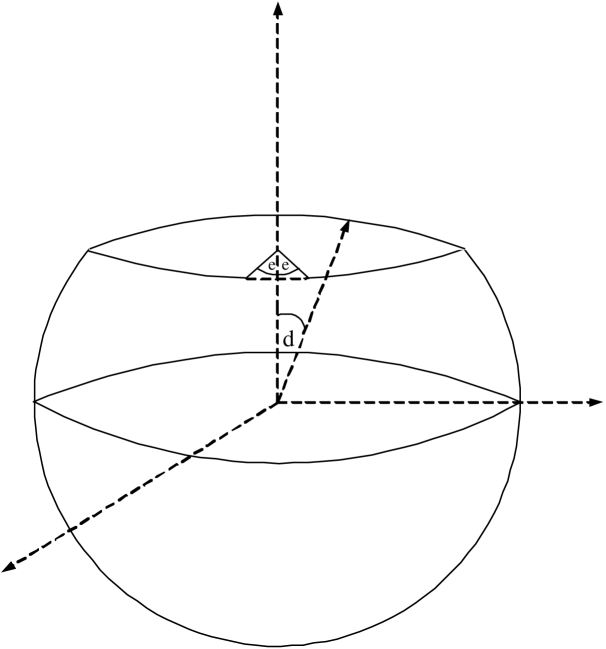
Figure 5: A sphere of radius $R$ without a spherical cap at the north pole of central angle $\delta$. The particle can exit through an arc seen at angle $2\varepsilon$.

Consider again a Brownian particle diffusing on a decapitated 3-sphere of radius $1/2$. The boundary of the spherical cap is reflecting but for a small window that is absorbing (see Fig. 5). We calculate the mean time to absorption. Using the stereographic projection of the preceding subsection, we obtain the mixed boundary value problem

$$\Delta v = -\frac{1}{(1+r^{2})^{2}},\quad\mbox{for}\quad r<r_{\delta},\quad 0\leq\phi<2\pi,$$

$$v(r,\phi)\bigg{|}_{r=r_{\delta}} = 0,\quad\mbox{for}\quad|\phi-\pi|<\varepsilon,$$

$$\frac{\partial v(r,\phi)}{\partial r}\bigg{|}_{r=r_{\delta}} = 0,\quad\mbox{for}\quad|\phi-\pi|>\varepsilon.$$ (6.15)

The function

$$w(r)=\frac{1}{4}\log\left(\displaystyle{\frac{1+r_{\delta}^{2}}{1+r^{2}}}\right)$$

is the solution of the all absorbing boundary problem eq.(6.13), so the function $u=v-w$ satisfies the mixed boundary value problem

$$\Delta u = 0,\quad r<r_{\delta},\quad\mbox{for}\quad 0\leq\phi<2\pi,$$

$$u(r,\phi)\bigg{|}_{r=r_{\delta}} = 0,\quad\mbox{for}\quad|\phi-\pi|<\varepsilon,$$

$$\frac{\partial u(r,\phi)}{\partial r}\bigg{|}_{r=r_{\delta}} = \frac{r_{\delta}}{2(1+r_{\delta}^{2})},\quad\mbox{for}\quad|\phi-\pi|>\varepsilon.$$ (6.16)

Scaling $\tilde{r}=r/r_{\delta}$, we find this mixed boundary value problem to be that of a planar disk [5], with the only difference that the constant $1/2$ is now replaced by $\displaystyle{\frac{r_{\delta}^{2}}{2(1+r_{\delta}^{2})}}$. Therefore, the solution is given by

$$a_{0}=-\frac{2r_{\delta}^{2}}{1+r_{\delta}^{2}}\left[\log\frac{\varepsilon}{2}+O(\varepsilon)\right].$$ (6.17)

Transforming back to the spherical coordinate system, the MFPT is

$$v(\theta,\phi) = \frac{1}{2}\log\frac{\sin\theta/2}{\sin\delta/2}$$

$$-\cos^{2}\frac{\delta}{2}\left[\log\frac{\varepsilon}{2}+O(\varepsilon)\right]+\sum_{n=1}^{\infty}a_{n}\left[\frac{\cot\left(\theta/2\right)}{\cot\left(\delta/2\right)}\right]^{n}\cos n\phi.$$

The MFPT, averaged over uniformly distributed initial conditions on the decapitated sphere, is

$$E\tau=-\frac{1}{2}\left(\frac{\log\sin(\delta/2)}{\cos^{2}(\delta/2)}+\frac{1}{2}\right)+\cos^{2}\frac{\delta}{2}\left[\log\frac{2}{\varepsilon}+O(\varepsilon)\right].$$ (6.19)

Scaling the radius $R$ of the sphere into (6.19), we find that for small $\varepsilon$ and $\delta$ the averaged MFPT is

$$E\tau=2R^{2}\left[\log\frac{1}{\delta}+2\log\frac{1}{\varepsilon}+3\log 2-\frac{1}{2}+O(\varepsilon,\delta^{2}\log\delta,\delta^{2}\log\varepsilon)\right].$$ (6.20)

There are two different contributions to the MFPT. The ratio $\varepsilon$ between the absorbing arc and the entire boundary brings in a logarithmic contribution to the MFPT, which is to leading order

$$\frac{|\Omega|_{g}}{\pi}\log\frac{1}{\varepsilon}.$$

However, the central angle $\delta$ gives an additional logarithmic contribution, of the form

$$\frac{|\Omega|_{g}}{2\pi}\log\frac{1}{\delta}.$$

The factor 2 difference in the asymptotic expansions is the same as encountered in the planar annulus problem.

The MFPT for a particle initiated at the south pole $\theta=\pi$ is

$$v(\pi) = -2R^{2}\log\sin\displaystyle{\frac{\delta}{2}}-4R^{2}\cos^{2}\frac{\delta}{2}\left[\log\frac{\varepsilon}{2}+O(\varepsilon)\right]$$ (6.21)

$$= 2R^{2}\left[\log\frac{1}{\delta}+2\log\frac{1}{\varepsilon}+3\log 2+O(\varepsilon,\delta^{2}\log\delta,\delta^{2}\log\varepsilon)\right].$$

We also find the location $(\theta,\phi)$ for which the MFPT is maximal. The stationarity condition $\displaystyle{\frac{\partial v}{\partial\phi}}=0$ implies that $\phi=0$, as expected (the opposite $\phi$-direction to the center of the window). The infinite sum in equation (LABEL:eq:MFPT-sphere-north) is $O(1)$. Therefore, for $\delta\ll 1$, the MFPT is maximal near the south pole $\theta=\pi$. However, for $\delta=O(1)$, the location of the maximal MFPT is more complex.

Finally, we remark that the stereographic projection also leads to the determination of the MFPT for diffusion on a 3-sphere with a small hole as discussed above, and an all reflecting spherical cap at the south pole. In this case, the image for the stereographic projection is the annulus, a problem solved in Section 3.

Appendix A Laplace Beltrami operator on 3-sphere

The Laplace Beltrami operator on a manifold is given by

$$\Delta_{M}f=\frac{1}{\sqrt{\det G}}\sum_{i,j}\frac{\partial}{\partial\xi_{i}}\left(g^{ij}\sqrt{\det G}\frac{\partial f}{\partial\xi_{j}}\right),$$ (A.1)

where

$$\mbox{\boldmath$t$}_{i}=\frac{\partial\mbox{\boldmath$r$}}{\partial\xi_{i}},\quad g_{ij}=\langle\mbox{\boldmath$t$}_{i},\mbox{\boldmath$t$}_{j}\rangle,\quad G=(g_{ij}),\quad g^{ij}=g_{ij}^{-1}.$$ (A.2)

In spherical coordinates we have

$$g_{\theta\theta}=R^{2},\quad g_{\phi\phi}=R^{2}\sin^{2}\theta,\quad g_{\theta\phi}=g_{\phi\theta}=0.$$ (A.3)

Therefore, for a function $w=w(\theta,\phi)$

$$\Delta_{M}f=R^{-2}\left(\frac{\partial^{2}f}{\partial\theta^{2}}+\cot\theta\,\frac{\partial f}{\partial\theta}+\frac{1}{\sin^{2}\theta}\frac{\partial^{2}f}{\partial\phi^{2}}\right).$$ (A.4)

Acknowledgment: This research was partially supported by research grants from the Israel Science Foundation, US-Israel Binational Science Foundation, and the NIH Grant No. UPSHS 5 RO1 GM 067241.

Figure 1: An annulus $R_{1}<r<R_{2}$. The particle is absorbed at an arc of length $2\varepsilon R_{1}$ (dashed line) at the inner circle. The solid lines indicate reflecting boundaries.

References

- [1] B. Hille, Ionic Channels of Excitable Membranes, 2nd ed., Sinauer, Mass., 1992.
- [2] D. Holcman, Z. Schuss, “Diffusion of receptors on a postsynaptic membrane: exit through a small opening”, J. Stat. Phys. (in print).
- [3] A.J. Borgdorff, D. Choquet, “Regulation of AMPA receptor lateral movements”, Nature 417 (6889), pp.649-53 (2002).
- [4] A. Singer, Z. Schuss, D. Holcman, R.S. Eisenberg, “Narrow Escape, Part I”, (preprint).
- [5] A. Singer, Z. Schuss, D. Holcman,“Narrow Escape, part II: The circular disk”, (preprint).
- [6] H.P. McKean, Jr., Stochastic Integrals, Academic Press, NY 1969.
- [7] Z. Schuss, Theory and Applications of Stochastic Differential Equations, Wiley Series in Probability and Statistics, Wiley, NY 1980.
- [8] P. R. Garabedian, Partial Differential Equations, Wiley, NY 1964.
- [9] T. Aubin, Some Nonlinear Problems in Riemannian Geometry, Springer, NY 1998,
- [10] V.A. Kozlov, V.G. Mazya and J. Rossmann, Elliptic Boundary Value Problems in Domains with Point Singularities, American Mathematical Society, Mathematical Surveys and Monographs, vol. 52, 1997.
- [11] I. N. Sneddon, Mixed Boundary Value Problems in Potential Theory, Wiley, NY, 1966.
- [12] V. I. Fabrikant, Applications of Potential Theory in Mechanics, Kluwer, 1989.
- [13] V. I. Fabrikant, Mixed Boundary Value Problems of Potential Theory and Their Applications in Engineering, Kluwer, 1991.
- [14] W. D. Collins, “On some dual series equations and their application to electrostatic problems for spheroidal caps”, Proc. Cambridge Phil. Soc. 57, pp. 367-384, 1961.
- [15] W. D. Collins, “Note on an electrified circular disk situated inside an earthed coaxial infinite hollow cylinder”, Proc. Cambridge Phil. Soc. 57, pp. 623-627, 1961.
- [16] B. Øksendal, Stochastic Differential Equations, 5th ed., Springer, Berlin Heidelberg, 1998.
- [17] E. Hille, Analytic Function Theory, vol. 1, Chelsea Publishing Company, New York, 1976.