Abstract

We consider Brownian motion in a circular disk $\Omega$, whose boundary $\partial\Omega$ is reflecting, except for a small arc, $\partial\Omega_{a}$, which is absorbing. As $\varepsilon=|\partial\Omega_{a}|/|\partial\Omega|$ decreases to zero the mean time to absorption in $\partial\Omega_{a}$, denoted $E\tau$, becomes infinite. The narrow escape problem is to find an asymptotic expansion of $E\tau$ for $\varepsilon\ll 1$. We find the first two terms in the expansion and an estimate of the error. The results are extended in a straightforward manner to planar domains and two-dimensional Riemannian manifolds that can be mapped conformally onto the disk. Our results improve the previously derived expansion for a general smooth domain, $E\tau=\displaystyle{\frac{|\Omega|}{D\pi}}\left[\log\displaystyle{\frac{1}{\varepsilon}}+O(1)\right],$ ($D$ is the diffusion coefficient) in the case of a circular disk. We find that the mean first passage time from the center of the disk is $E[\tau\,|\,\mbox{\boldmath$x$}(0)=\mbox{\boldmath$0$}]=\displaystyle{\frac{R^{2}}{D}}\left[\log\displaystyle{\frac{1}{\varepsilon}}+\log 2+\displaystyle{\frac{1}{4}}+O(\varepsilon)\right]$. The second term in the expansion is needed in real life applications, such as trafficking of receptors on neuronal spines, because $\log\displaystyle{\frac{1}{\varepsilon}}$ is not necessarily large, even when $\varepsilon$ is small. We also find the singular behavior of the probability flux profile into $\partial\Omega_{a}$ at the endpoints of $\partial\Omega_{a}$, and find the value of the flux near the center of the window.

1 Introduction

The expected lifetime of a Brownian motion in a bounded domain, whose boundary is reflecting, except for a small absorbing portion, increases indefinitely as the absorbing part shrinks to zero. The narrow escape problem is to find an asymptotic expansion of the expected lifetime of the Brownian motion in this limit. The narrow escape problem in three dimensions has been studied in the first paper of this series [1], where is was converted to a mixed Dirichlet-Neumann boundary value problem for the Poisson equation in the domain. This is a well known problem of classical electrostatics (e.g., the electrified disk problem [2]), elasticity (punch problems), diffusion and conductance theory, hydrodynamics, and acoustics [3]-[7]. It dates back to Helmholtz [8] and Lord Rayleigh [9] and has been extensively studied in the literature for special geometries.

The study of the two-dimensional narrow escape problem began in [10] in the context of receptor trafficking on biological membranes [11], where a leading order expansion of the expected lifetime was constructed for a general smooth planar domain. In this paper we present a thorough analysis of the narrow escape problem for the circular disk and note that our calculations apply in a straightforward manner to any simply connected domain in the plane that can be mapped conformally onto the disk. According to Riemann’s mapping theorem [12], this covers all simply connected planar domains whose boundary contains at least one point. The same conclusion holds for the narrow escape problem on two-dimensional Riemannian manifolds that are conformally equivalent to a circular disk. The biological problem of receptor trafficking on membranes is locally planar, but globally it is a problem on a Riemannian manifold. The narrow escape problem of non-smooth domains that contain corners or cusp points at their boundary is treated in the third part of this series [13], where the conformal mapping method is demonstrated.

The specific mathematical problem can be formulated as follows. A Brownian particle diffuses freely in a disk $\Omega$, whose boundary $\partial\Omega$ is reflecting, except for a small absorbing arc $\partial\Omega_{a}$. The ratio between the arclength of the absorbing boundary and the arclength of the entire boundary is a small parameter

$$\varepsilon=\displaystyle{\frac{|\partial\Omega_{a}|}{|\partial\Omega|}}\ll 1.$$

The mean first passage time to $\partial\Omega_{a}$, denoted $E\tau$, becomes infinite as $\varepsilon\to 0$. The asymptotic expansion of $E\tau$ for $\varepsilon\ll 1$ was considered for the particular case when $\partial\Omega_{a}$ is a disjoint component of $\partial\Omega$ in [14, and references therein]. This case differs from the case at hand in that the absorption probability flux density in the former is regular, while in the latter it is singular. It was shown in [10] that $E\tau$ for the narrow escape problem in a general planar domain $\Omega$ has the asymptotic form

$$E\tau=\displaystyle{\frac{|\Omega|}{D\pi}}\left[\log\frac{1}{\varepsilon}+O(1)\right],$$ (1.1)

where $|\Omega|$ is the area of $\Omega$, and $D$ is the diffusion coefficient. This leading order asymptotics has the drawback that $\log\varepsilon$ can be $O(1)$ when $\varepsilon\ll 1$. Thus the second term in the expansion is needed. For the particular case of a circular disk an approximate value for the correction was given in [10]. In contrast, the asymptotics of $E\tau$ for a three dimensional ball of radius $R$ with an absorbing window of radius $\varepsilon R$ is [1]

$$E\tau=\displaystyle{\frac{|\Omega|}{4D\varepsilon R}}\left[1+O(\varepsilon\log\varepsilon)\right],$$

so the leading order term is much larger than the correction term if $\varepsilon$ is small. The difference in the asymptotic form of $E\tau$ stems from the different singularities of the Neumann function in two and three dimensions: it is logarithmic in two dimensions and has a pole in three dimensions.

Our computations are based on the mixed boundary value techniques of [3]. They reveal the singularity of the absorption flux in the absorbing arc $\partial\Omega_{a}$. Specifically, the singularity is $(\varepsilon^{2}-s^{2})^{-1/2}$, where $s$ is the (dimensionless) arclength measured from the center of $\partial\Omega_{a}$, and attains the values $s=\pm\varepsilon$ at the endpoints.

The exit time vanishes at the absorbing boundary, and is small near the absorbing boundary, but it attains large and almost constant values of order $\log\displaystyle{\frac{1}{\varepsilon}}$ inside the domain. We show that this “jump” occurs in a small boundary layer of size $O\left(\varepsilon\log\displaystyle{\frac{1}{\varepsilon}}\right)$. We calculate the average exit time, where the averaging is against a uniform initial distribution in the disk, the time to exit from the center, and the maximum mean exit time, attained at the antipodal point to the center of the absorbing window.

The mean first passage time (MFPT) from the center of the disk is

$$E[\tau\,|\,\mbox{\boldmath$x$}(0)=\mbox{\boldmath$0$}]=\frac{R^{2}}{D}\left[\log\frac{1}{\varepsilon}+\log 2+\frac{1}{4}+O(\varepsilon)\right],$$ (1.2)

the MFPT, averaged with respect to an initial uniform distribution in the disk is

$$E\tau=\frac{R^{2}}{D}\left[\log\frac{1}{\varepsilon}+\log 2+\frac{1}{8}+O(\varepsilon)\right],$$ (1.3)

and the maximal value of the MFPT is attained on the circumference, at the antipodal point to the center of the hole,

$$\max_{\mbox{\boldmath$x$}\in\Omega}E[\tau\,|\,\mbox{\boldmath$x$}]=E[\tau\,|\,r=1,\theta=0]=\frac{R^{2}}{D}\left[\log\frac{1}{\varepsilon}+2\log 2+O(\varepsilon)\right].$$ (1.4)

The boundary layer analysis of $E\tau$ can be applied to the approximation of the first eigenfunction and eigenvalue of the mixed Neumann-Dirichlet boundary value problem with a small Dirichlet window on the boundary. This problem arises in the construction of the first eigenfunction and eigenvalue of the Neumann problem in a domain that consists of two domains (e.g., circular disks) connected by a narrow channel [15], [16].

Specifically, it is easy to see that

$$E\tau=\sum_{n=0}^{\infty}\frac{1}{\lambda_{n}}\sim\frac{1}{\lambda_{0}}\,$$ (1.5)

where $0<\lambda_{0}\ll\lambda_{1}<\cdots$ are the eigenvalues of the mixed problem and the MFPT is also averaged with respect to the initial point. The first eigenfunction $u_{0}$ of the mixed problem is differs from the first eigenfunction of the Neumann problem, which is $v_{0}=1$, only in a boundary layer about the small window. Thus $u_{0}$ is a small perturbation (in $L^{2}$ norm) of $v_{0}=1$. It follow that $u_{0}/\lambda_{0}$ differs from $E\tau$ only in the boundary layer.

2 Solution of a mixed boundary value problem

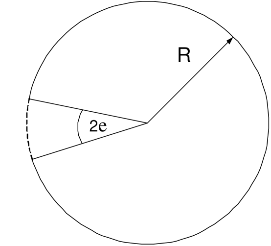
Figure 1: A circular disk of radius $R$. The arclength of the absorbing boundary (dashed line) is $2\varepsilon R$. The solid line indicates the reflecting boundary.

In non-dimensional variables the narrow escape problem concerns Brownian motion inside the unit disk, whose boundary is reflecting but for a small absorbing arc of length $2\varepsilon$ (see Fig.1). In polar coordinates $\mbox{\boldmath$x$}=(r,\theta)$ the MFPT

$$v(r,\theta)=E[\tau\,|\,\mbox{\boldmath$x$}(0)=(r,\theta)],$$

is the solution to the mixed Neumann-Dirichlet inhomogeneous boundary value problem (see, e.g. [17])

$$\Delta v(r,\theta) = -1,\quad r<1,\quad\mbox{for}\quad 0\leq\theta<2\pi,$$

$$v(r,\theta)\bigg{|}_{r=1} = 0,\quad\mbox{for}\quad|\theta-\pi|<\varepsilon,$$

$$\frac{\partial v(r,\theta)}{\partial r}\bigg{|}_{r=1} = 0,\quad\mbox{for}\quad|\theta-\pi|\rangle\varepsilon,$$ (2.1)

which is reduced by the substitution

$$u=v-\frac{1-r^{2}}{4}$$ (2.2)

to the mixed Neumann-Dirichlet problem for the Laplace equation

$$\Delta u(r,\theta) = 0,\quad\mbox{for}\quad r<1,\quad 0\leq\theta<2\pi,$$

$$u(r,\theta)\bigg{|}_{r=1} = 0,\quad\mbox{for}\quad|\theta-\pi|<\varepsilon,$$ (2.3)

$$\frac{\partial u(r,\theta)}{\partial r}\bigg{|}_{r=1} = \frac{1}{2},\quad\mbox{for}\quad|\theta-\pi|\rangle\varepsilon.$$

We adapt the method of [3] to the solution of (2.3). Separation of variables suggests that

$$u(r,\theta)=\frac{a_{0}}{2}+\sum_{n=1}^{\infty}a_{n}r^{n}\cos n\theta,$$ (2.4)

where the coefficients $\{a_{n}\}$ are to be determined by the boundary conditions

$$u(r,\theta)\bigg{|}_{r=1} = \frac{a_{0}}{2}+\sum_{n=1}^{\infty}a_{n}\cos n\theta=0,\quad\mbox{for}\quad\pi-\varepsilon<\theta\leq\pi,$$ (2.5)

$$\frac{\partial u(r,\theta)}{\partial r}\bigg{|}_{r=1} = \sum_{n=1}^{\infty}na_{n}\cos n\theta=\frac{1}{2},\quad\mbox{for}\quad 0\leq\theta<\pi-\varepsilon.$$ (2.6)

We identify this problem with problem (5.4.4) in [3], where general functions appear on the right hand sides of equations (2.5) (2.6). Due to the invertibility of Abel’s integral operator, the equation

$$\frac{a_{0}}{2}+\sum_{n=1}^{\infty}a_{n}\cos n\theta=\cos\frac{1}{2}\theta\int_{\theta}^{\pi-\varepsilon}\frac{h_{1}(t)\,dt}{\sqrt{\cos\theta-\cos t}},$$ (2.7)

defines $h_{1}(t)$ uniquely for $0\leq t<\pi-\varepsilon$. The coefficients are given by

$$a_{n} = \frac{2}{\pi}\int_{0}^{\pi-\varepsilon}\cos n\theta\cos\frac{1}{2}\theta\,d\theta\int_{\theta}^{\pi-\varepsilon}\frac{h_{1}(t)\,dt}{\sqrt{\cos\theta-\cos t}}$$ (2.8)

$$= \frac{1}{\pi}\int_{0}^{\pi-\varepsilon}h_{1}(t)\,dt\int_{0}^{t}\frac{\cos\left(n+\frac{1}{2}\right)\theta+\cos\left(n-\frac{1}{2}\right)\theta}{\sqrt{\cos\theta-\cos t}}\,d\theta.$$

The integral

$$P_{n}(\cos u)=\frac{\sqrt{2}}{\pi}\int_{0}^{u}\frac{\cos\left(n+\frac{1}{2}\right)\theta}{\sqrt{\cos\theta-\cos u}}\,d\theta,$$ (2.9)

is Mehler’s integral representation of representation of the Legendre polynomial [19]. It follows that

$$a_{n}=\frac{1}{\sqrt{2}}\int_{0}^{\pi-\varepsilon}h_{1}(t)[P_{n}(\cos t)+P_{n-1}(\cos t)]\,dt,$$ (2.10)

for $n>0$, and

$$a_{0}=\frac{2}{\pi}\int_{0}^{\pi-\varepsilon}h_{1}(t)\,dt\int_{0}^{t}\frac{\cos\frac{1}{2}\theta}{\sqrt{\cos\theta-\cos t}}\,d\theta=\sqrt{2}\int_{0}^{\pi-\varepsilon}h_{1}(t)\,dt.$$ (2.11)

Integration of (2.6) gives

$$\sum_{n=1}^{\infty}a_{n}\sin n\theta=\frac{1}{2}\theta,\quad\mbox{for}\quad 0\leq\theta<\pi-\varepsilon.$$ (2.12)

Changing the order of summation and integration yields

$$\int_{0}^{\pi-\varepsilon}h_{1}(t)\frac{1}{\sqrt{2}}\sum_{n=1}^{\infty}[P_{n}(\cos t)+P_{n-1}(\cos t)]\sin n\theta\,dt=\frac{1}{2}\theta.$$ (2.13)

Using [3, eq.(2.6.31)],

$$\frac{1}{\sqrt{2}}\sum_{n=1}^{\infty}[P_{n}(\cos t)+P_{n-1}(\cos t)]\sin n\theta=\frac{\cos\frac{1}{2}\theta H(\theta-t)}{\sqrt{\cos t-\cos\theta}},$$ (2.14)

we obtain

$$\int_{0}^{\theta}\frac{h_{1}(t)\,dt}{\sqrt{\cos t-\cos\theta}}=\frac{\theta}{2\cos\frac{1}{2}\theta},\quad\mbox{for}\quad 0\leq\theta<\pi-\varepsilon.$$ (2.15)

The solution of the Abel-type integral equation (2.15) is given by

$$h_{1}(t)=\frac{1}{\pi}\frac{d}{dt}\int_{0}^{t}\frac{u\sin\displaystyle{\frac{u}{2}}}{\sqrt{\cos u-\cos t}}\,du.$$ (2.16)

Together with (2.11) this gives

$$a_{0}=\frac{\sqrt{2}}{\pi}\int_{0}^{\pi-\varepsilon}\frac{u\sin\displaystyle{\frac{u}{2}}}{\sqrt{\cos u+\cos\varepsilon}}\,du.$$ (2.17)

We expect the function $u(r,\theta)$, closely related to the MFPT, to be almost constant in the disk, except for a boundary layer near the absorbing arc. The value of this constant is $a_{0}$, because all other terms of expansion (2.4) are oscillatory.

2.1 Small $\varepsilon$ asymptotics

The results of the previous section are independent of the value of $\varepsilon$. Here we find the asymptotic of $a_{0}$ for $\varepsilon\ll 1$. Substituting

$$s=\sqrt{\frac{\cos u+\cos\varepsilon}{2}}$$ (2.18)

in the integral (2.17) yields

$$a_{0} = \frac{4}{\pi}\int_{0}^{\cos(\varepsilon/2)}\frac{\arccos\sqrt{s^{2}+\sin^{2}\displaystyle{\frac{\varepsilon}{2}}}}{\sqrt{s^{2}+\sin^{2}\displaystyle{\frac{\varepsilon}{2}}}}\,ds$$ (2.19)

$$= 2\int_{0}^{\cos(\varepsilon/2)}\frac{1}{\sqrt{s^{2}+\sin^{2}\frac{\varepsilon}{2}}}\,ds-\frac{4}{\pi}\int_{0}^{\cos(\varepsilon/2)}\frac{\arcsin\sqrt{s^{2}+\sin^{2}\displaystyle{\frac{\varepsilon}{2}}}}{\sqrt{s^{2}+\sin^{2}\displaystyle{\frac{\varepsilon}{2}}}}\,ds$$

$$= 2\log\left(1+\cos\frac{\varepsilon}{2}\right)-2\log\sin\frac{\varepsilon}{2}-\frac{4}{\pi}\int_{0}^{\cos(\varepsilon/2)}\frac{\arcsin\sqrt{s^{2}+\sin^{2}\displaystyle{\frac{\varepsilon}{2}}}}{\sqrt{s^{2}+\sin^{2}\displaystyle{\frac{\varepsilon}{2}}}}\,ds$$

$$= -2\log\frac{\varepsilon}{2}+2\log 2-\frac{4}{\pi}\int_{0}^{1}\frac{\arcsin s}{s}\,ds+O(\varepsilon)$$

$$= -2\log\frac{\varepsilon}{2}+O(\varepsilon),$$

because $\displaystyle{\int_{0}^{1}\frac{\arcsin s}{s}}\,ds=\displaystyle{\frac{\pi}{2}}\log 2$. The substitution (2.18) turns out to be extremely useful in evaluating the integrals appearing here.

2.2 Expected lifetime

Now, that we have the asymptotic expansion of $a_{0}$ (eq.(2.19)), the evaluation of expected lifetime (MFPT to the absorbing boundary $\partial\Omega_{a}$) becomes possible. Setting $r=0$ in equations (2.2) and (2.4), we obtain the expression (1.2) for MFPT from the center of the disk.

Averaging (2.3) with respect to a uniform initial distribution in $\Omega$ gives

$$E\tau = \frac{1}{\pi}\int_{0}^{2\pi}\,d\theta\int_{0}^{1}v(r,\theta)r\,dr=\int_{0}^{1}\left[\left(a_{0}+\frac{1}{2}\right)r-\frac{r^{3}}{2}\right]\,dr$$ (2.20)

$$= \frac{a_{0}}{2}+\frac{1}{8}=-\log\frac{\varepsilon}{2}+\frac{1}{8},$$

as asserted in eq.(1.3).

The maximal value of the MFPT is attained at the point $r=1,\theta=0$, which is antipodal to the center of the absorbing arc. At this point $\displaystyle{\frac{\partial u}{\partial\theta}}=0$, as can be seen by differentiating expansion (2.4) term by term. Setting $r=1$ and $\theta=0$, we find that

$$v_{max}=u(1,0)=\frac{a_{0}}{2}+\sum_{n=1}^{\infty}a_{n}.$$ (2.21)

The evaluation of the maximal exit time is not as straightforward as the previous evaluated MFPTs, because one needs to calculate the infinite sum in (2.21). This calculation is done in Appendix A, where we find (eq.(A.12))

$$v_{max}=\log\frac{1}{\varepsilon}+2\log 2+O(\varepsilon),$$

as asserted in equation (1.4).

2.3 Boundary layers

We see that the maximal exit time is only $v_{max}-v_{center}=\log 2-\displaystyle{\frac{1}{4}}=.4431471806\ldots$ longer than its value at the center of the disk. In other words, the variance along the radius $\theta=0,\,0\leq r\leq 1$ is very small. However, in the opposite direction $\theta=\pi,\,0\leq r\leq 1$, we expect a much different behavior. In particular, the MFPT is decreasing from a value of $v_{center}\approx\log\displaystyle{\frac{1}{\varepsilon}}$ at the center of the disk to $v(1,\pi)=0$ at the center of $\partial\Omega_{a}$. The calculation of the exit time

$$v_{ray}(r)\equiv v(r,\theta=\pi)=\frac{1-r^{2}}{4}+\frac{a_{0}}{2}+\sum_{n=1}^{\infty}a_{n}(-r)^{n},$$ (2.22)

is similar to that of the maximal exit time and is done in Appendix B. For $\varepsilon\ll 1$ and $1-r\gg\sqrt{\varepsilon}$, we find the asymptotic form (eq.(B.8))

$$v_{ray}(r)=-\log\frac{\varepsilon}{2}+2\log(1-r)+\frac{1-r^{2}}{4}-\log(1+r^{2})+q(r)+O(\varepsilon),$$ (2.23)

where $q(r)$ is a smooth function in the interval $[0,1]$ (eqs.(B.6)-(B.7)). Clearly, this asymptotic expansion does not hold all the way through to the absorbing arc at $r=1$, where the boundary condition requires $v_{ray}(r=1)\,=0$. Instead, the boundary condition is almost satisfied at $r=1-\sqrt{\displaystyle{\frac{\varepsilon}{2}}}$

$$v_{ray}\left(1-\sqrt{\frac{\varepsilon}{2}}\,\right)=-\log\frac{\varepsilon}{2}+2\log\left(\sqrt{\frac{\varepsilon}{2}}\right)+O(\varepsilon)=O(\varepsilon),$$ (2.24)

In other words, the asymptotic series (2.23) is the outer expansion [18].

We proceed to construct the boundary layer for $1-r\ll\sqrt{\varepsilon}$. Setting $\delta=1-r$, we have the identities

$$\frac{1-r^{2}}{4} = \frac{1}{2}\delta-\frac{1}{4}\delta^{2},$$

$$1-2r\cos\varepsilon+r^{2} = 4\sin^{2}\frac{\varepsilon}{2}\,(1-\delta)+\delta^{2}.$$

The exact form of the MFPT along the ray, eq.(B.3), gives the expansion

$$v_{ray}(\delta) = \frac{\delta}{2}+\frac{a_{0}\delta}{4\sin\displaystyle{\frac{\varepsilon}{2}}}$$

$$-\frac{\delta}{\pi\sin\displaystyle{\frac{\varepsilon}{2}}}\int_{0}^{\cos(\varepsilon/2)}\frac{\arccos\sqrt{s^{2}+\sin^{2}\displaystyle{\frac{\varepsilon}{2}}}\ s^{2}\,ds}{\left(s^{2}+\sin^{2}\displaystyle{\frac{\varepsilon}{2}}\right)^{3/2}}+O\left(\frac{\delta^{2}}{\varepsilon}\right).$$

Evaluating the integral in eq.(2.3),

$$\int_{0}^{\cos(\varepsilon/2)}\frac{\arccos\sqrt{s^{2}+\sin^{2}\displaystyle{\frac{\varepsilon}{2}}}\ s^{2}\,ds}{\left(s^{2}+\sin^{2}\displaystyle{\frac{\varepsilon}{2}}\right)^{3/2}}$$

$$=-\frac{\pi}{2}\left[\log\sin\displaystyle{\frac{\varepsilon}{2}}+\cos\frac{\varepsilon}{2}-\log\left(1+\cos\frac{\varepsilon}{2}\right)+\log 2\right]+O(\varepsilon),$$ (2.26)

we obtain the boundary layer structure

$$v_{ray}(\delta) = \frac{\delta}{\varepsilon}+O\left(\delta,\,\frac{\delta^{2}}{\varepsilon}\right).$$ (2.27)

In particular, setting $\delta_{0}=-\varepsilon\log\displaystyle{\frac{\varepsilon}{2}}$ yields

$$v_{ray}(\delta_{0})=-\log\frac{\varepsilon}{2}+O(\varepsilon\log^{2}\varepsilon),$$ (2.28)

which is the value of the outer solution. We conclude that the width of the boundary layer is $O\left(\varepsilon\log\displaystyle{\frac{1}{\varepsilon}}\right)$. Furthermore, the flux at the center of the hole is given by

$$\mbox{flux}_{\mbox{center}}=\frac{\partial v_{ray}}{\partial r}\bigg{|}_{r=1}=-\frac{\partial v_{ray}}{\partial\delta}\bigg{|}_{\delta=0}=-\frac{1}{\varepsilon}+O(1).$$ (2.29)

2.4 Flux profile

Next, we calculate the profile of the flux on the absorbing arc. Differentiating expansion (2.4) gives the flux as

$$f(\theta)=\frac{\partial v(r,\theta)}{\partial r}\bigg{|}_{r=1}=\frac{\partial u(r,\theta)}{\partial r}\bigg{|}_{r=1}-\frac{1}{2}=-\frac{1}{2}+\sum_{n=1}^{\infty}na_{n}\cos n\theta,$$ (2.30)

for $\pi-\varepsilon<\theta\leq\pi$. Using equation (2.10) for the coefficients, we have

$$f(\theta) = -\frac{1}{2}+\frac{1}{\sqrt{2}}\int_{0}^{\pi-\varepsilon}h_{1}(t)\,dt\sum_{n=1}^{\infty}n[P_{n}(\cos t)+P_{n-1}(\cos t)]\cos n\theta$$

$$= -\frac{1}{2}+\frac{1}{\sqrt{2}}\frac{d}{d\theta}\int_{0}^{\pi-\varepsilon}h_{1}(t)\,dt\sum_{n=1}^{\infty}[P_{n}(\cos t)+P_{n-1}(\cos t)]\sin n\theta.$$

Since $\theta\rangle\pi-\varepsilon\rangle t$, equation (2.14) implies

$$f(\theta)=-\frac{1}{2}+\frac{d}{d\theta}\left(\cos\frac{\theta}{2}\int_{0}^{\pi-\varepsilon}\frac{h_{1}(t)\,dt}{\sqrt{\cos t-\cos\theta}}\right).$$ (2.31)

The evaluation of this integral is not immediate and is given in Appendix C. We find that (eq.(C.17))

$$f(\alpha) = -\frac{\alpha^{2}}{\varepsilon\sqrt{1-\alpha^{2}}}-\frac{1}{\varepsilon}\sum_{n=0}^{\infty}\left(\frac{\left(2^{n+1}(n+1)!\right)^{2}}{(2n+2)!}\alpha^{2}-\frac{(2^{n}n!)^{2}}{(2n+1)!}\right)(1-\alpha^{2})^{n+1/2}$$ (2.32)

$$-\frac{\pi}{2\varepsilon}\sum_{n=0}^{\infty}\left(\frac{(2n)!}{(2^{n}n!)^{2}}-\frac{(2n+2)!(2n+2)}{(2^{n+1}(n+1)!)^{2}}\alpha^{2}\right)(1-\alpha^{2})^{n}+O(1),$$

where $\alpha=\displaystyle{\frac{\pi-\theta}{\varepsilon}},\,|\alpha|<1$. The flux has a singular part, represented by the half-integer powers of $(1-\alpha^{2}$), and a remaining regular part (the integer powers.) The first term, $-\displaystyle{\frac{\alpha^{2}}{\varepsilon\sqrt{1-\alpha^{2}}}}$, is the most singular one, because it becomes infinite as $|\alpha|\rightarrow 1$. In other words, the flux is infinitely large near the boundary of the hole. The splitting of the solution into singular and regular parts is common in the theory of elliptic boundary value problems in domains with corners (see e.g., [20]-[22]).

The value of the flux at the center of the hole is to leading order

$$f(0) = -\frac{1}{\varepsilon}\sum_{n=0}^{\infty}\left(\frac{\pi}{2}\frac{(2n)!}{(2^{n}n!)^{2}}-\frac{(2^{n}n!)^{2}}{(2n+1)!}\right)=-\frac{1}{\varepsilon},$$ (2.33)

in agreement with (2.29) (thanks Maple for calculating the infinite sum.)

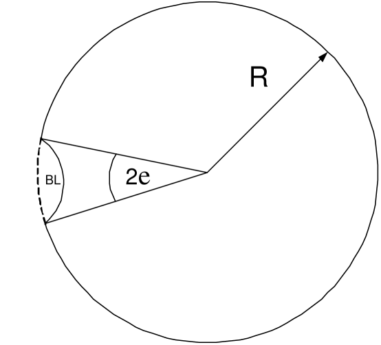
Figure 2: The boundary layer, indicated by “BL”, is the area bounded by the absorbing boundary (dashed line) and the solid arc. Outside the boundary layer the MFPT is $O\left(\log\displaystyle{\frac{1}{\varepsilon}}\right)$.

The size of the boundary layer is varying with $\theta$ proportionally to $1/f(\theta)$. The singularity at the end points of the hole indicate that the layer shrinks there to zero. Therefore, the boundary layer is shaped as a small cap bounded by the absorbing arc and (more or less) the curve $\sqrt{1-\alpha^{2}}$ (see Fig.2). In particular, the MFPT on the reflecting boundary is $O\left(\log\displaystyle{\frac{1}{\varepsilon}}\right)$, even when taken arbitrarily close to the absorbing boundary. The singularity of the flux near the endpoints indicates that the diffusive particle prefers to exit near the endpoints rather than through the center of the hole.

The expansion (C.17) is useful in approximating the flux near the endpoints $(\alpha=\pm 1)$, where few terms are needed. However, it is slowly converging near the center of the hole, where a power series in $\alpha^{2}$ should be used instead

$$f(\alpha)=\sum_{n=0}^{\infty}f_{n}\alpha^{2n}+O(1),$$ (2.34)

where the coefficients $f_{n}$ are $O(\varepsilon^{-1})$. Equations (2.33) and (2.29) indicate that $f_{0}=-\displaystyle{\frac{1}{\varepsilon}}$. All other coefficients can be found in a similar fashion. We conclude that near the center $(\alpha\ll 1)$ we have

$$f(\alpha)=-\frac{1}{\varepsilon}+O\left(1,\frac{\alpha^{2}}{\varepsilon}\right).$$ (2.35)

Appendix A Maximal exit time for the circular disk

Using equation (2.10) we find

$$v_{max} = u(1,0)=\frac{a_{0}}{2}+\sum_{n=1}^{\infty}a_{n}$$

$$= \frac{a_{0}}{2}+\frac{1}{\sqrt{2}}\int_{0}^{\pi-\varepsilon}h_{1}(t)\sum_{n=1}^{\infty}[P_{n}(\cos t)+P_{n-1}(\cos t)]\,dt.$$

Recall the generating function of the Legendre polynomials [19]

$$\frac{1}{\sqrt{1-2tx+t^{2}}}=\sum_{n=0}^{\infty}P_{n}(x)t^{n},$$ (A.2)

from which it follows that

$$\sum_{n=0}^{\infty}P_{n}(\cos t)=\frac{1}{\sqrt{1-2\cos t+1}}=\frac{1}{2\sin\displaystyle{\frac{t}{2}}}.$$ (A.3)

Together with equation (2.11), this gives

$$v_{max}=\frac{a_{0}}{2}+\frac{1}{\sqrt{2}}\int_{0}^{\pi-\varepsilon}h_{1}(t)\left(\frac{1}{\sin\displaystyle{\frac{t}{2}}}-1\right)\,dt=\frac{1}{\sqrt{2}}\int_{0}^{\pi-\varepsilon}\frac{h_{1}(t)\,dt}{\sin\displaystyle{\frac{t}{2}}}.$$ (A.4)

Combining with equation (2.16) and integrating by parts, we get

$$v_{max} = \frac{1}{\sqrt{2}}\int_{0}^{\pi-\varepsilon}\frac{1}{\pi}\frac{1}{\sin\displaystyle{\frac{t}{2}}}\frac{d}{dt}\int_{0}^{t}\frac{u\sin\displaystyle{\frac{u}{2}}\,du}{\sqrt{\cos u-\cos t}}\,dt$$

$$= \frac{1}{\sqrt{2}\pi\sin\displaystyle{\frac{t}{2}}}\int_{0}^{t}\frac{u\sin\displaystyle{\frac{u}{2}}\,du}{\sqrt{\cos u-\cos t}}\bigg{|}_{0}^{\pi-\varepsilon}$$

$$+\frac{1}{2\sqrt{2}\pi}\int_{0}^{\pi-\varepsilon}\frac{\cos\displaystyle{\frac{t}{2}}}{\sin^{2}\displaystyle{\frac{t}{2}}}\,dt\int_{0}^{t}\frac{u\sin\displaystyle{\frac{u}{2}}\,du}{\sqrt{\cos u-\cos t}}.$$

Equations (2.17) and (2.19) show that

$$\frac{\sqrt{2}}{\pi}\int_{0}^{t}\frac{u\sin\displaystyle{\frac{u}{2}}\,du}{\sqrt{\cos u-\cos t}}=-2\log\cos\frac{t}{2}+2\log\left(1+\sin\displaystyle{\frac{t}{2}}\right)+k(t),$$ (A.6)

where

$$k(t)=-\frac{4}{\pi}\int_{0}^{\displaystyle{\sin\frac{t}{2}}}\left(\frac{\arcsin\sqrt{s^{2}+\cos^{2}{\frac{t}{2}}}}{\sqrt{s^{2}+\cos^{2}\displaystyle{\frac{t}{2}}}}\right)\,ds.$$ (A.7)

Therefore,

$$\lim_{t\rightarrow 0}\frac{\sqrt{2}}{\pi\sin\displaystyle{\frac{t}{2}}}\int_{0}^{t}\frac{u\sin\displaystyle{\frac{u}{2}}\,du}{\sqrt{\cos u-\cos t}} = \lim_{t\rightarrow 0}\frac{-2\log\cos\displaystyle{\frac{t}{2}}+2\log\left(1+\sin\displaystyle{\frac{t}{2}}\right)+k(t)}{\sin\displaystyle{\frac{t}{2}}}$$ (A.8)

$$= 2-\frac{4}{\pi}\arcsin(1)=0.$$

Hence

$$v_{max}=$$

$$\frac{1}{2\cos\displaystyle{\frac{\varepsilon}{2}}}\left[2\log\left(1+\displaystyle{\cos\frac{\varepsilon}{2}}\right)-2\log\sin\displaystyle{\frac{\varepsilon}{2}}-\frac{4}{\pi}\int_{0}^{\displaystyle{\cos\frac{\varepsilon}{2}}}\left(\frac{\arcsin\sqrt{s^{2}+\sin^{2}\displaystyle{\frac{\varepsilon}{2}}}}{\sqrt{s^{2}+\sin^{2}\displaystyle{\frac{\varepsilon}{2}}}}\right)\,ds\right]$$

$$+\frac{1}{2\sqrt{2}\pi}\int_{0}^{\pi-\varepsilon}\frac{\cos\displaystyle{\frac{t}{2}}}{\sin^{2}\displaystyle{\frac{t}{2}}}\,dt\int_{0}^{t}\frac{u\sin\displaystyle{\frac{u}{2}}\,du}{\sqrt{\cos u-\cos t}}.$$

For $\varepsilon\ll 1$

$$v_{max}=-\log\frac{\varepsilon}{2}+\frac{1}{2\sqrt{2}\pi}\int_{0}^{\pi}\frac{\cos\displaystyle{\frac{t}{2}}}{\sin^{2}\displaystyle{\frac{t}{2}}}\,dt\int_{0}^{t}\frac{u\sin\displaystyle{\frac{u}{2}}\,du}{\sqrt{\cos u-\cos t}}+O(\varepsilon).$$ (A.9)

Changing the order of integration, we get

$$v_{max}=-\log\frac{\varepsilon}{2}+\frac{1}{2\sqrt{2}\pi}\int_{0}^{\pi}u\sin\displaystyle{\frac{u}{2}}\,du\int_{u}^{\pi}\frac{\cos\displaystyle{\frac{t}{2}}\,dt}{\sin^{2}\displaystyle{\frac{t}{2}}\sqrt{\cos u-\cos t}}+O(\varepsilon).$$ (A.10)

Substituting

$$s=\sqrt{\frac{\cos u-\cos t}{2}}$$ (A.11)

in the inner integral results in

$$\int_{u}^{\pi}\frac{\cos\displaystyle{\frac{t}{2}}\,dt}{\sin^{2}\displaystyle{\frac{t}{2}}\sqrt{\cos u-\cos t}}=\sqrt{2}\frac{\cos\displaystyle{\frac{u}{2}}}{\sin^{2}\displaystyle{\frac{u}{2}}}.$$

Therefore,

$$v_{max} = -\log\frac{\varepsilon}{2}+\frac{1}{2\pi}\int_{0}^{\pi}\frac{u}{\tan\displaystyle{\frac{u}{2}}}\,du=-\log\frac{\varepsilon}{2}-\frac{2}{\pi}\int_{0}^{\pi/2}\log\sin v\,dv$$ (A.12)

$$= -\log\frac{\varepsilon}{2}+\log 2.$$

Appendix B Exit times along the ray

Along the ray $\theta=\pi$ the MFPT is given by

$$v_{ray}(r) \equiv v(r,\theta=\pi)=\frac{1-r^{2}}{4}+\frac{a_{0}}{2}+\sum_{n=1}^{\infty}a_{n}(-r)^{n}$$

$$= \frac{1-r^{2}}{4}+\frac{a_{0}}{2}+\frac{1}{\sqrt{2}}\int_{0}^{\pi-\varepsilon}h_{1}(t)\sum_{n=1}^{\infty}[P_{n}(\cos t)+P_{n-1}(\cos t)](-r)^{n}\,dt.$$

Using the generating function (A.2) of the Legendre polynomials to sum the infinite series, we obtain

$$v_{ray}(r)=\frac{1-r^{2}}{4}+\frac{1-r}{\sqrt{2}}\int_{0}^{\pi-\varepsilon}\frac{h_{1}(t)\,dt}{\sqrt{1+2r\cos t+r^{2}}}.$$ (B.1)

Combining with equation (2.16), integrating by parts, and hanging the order of integration gives

$$v_{ray}(r)=\frac{1-r^{2}}{4}+\frac{1-r}{2\sqrt{1-2r\cos\varepsilon+r^{2}}}\,a_{0}$$

$$-\frac{r(1-r)}{\sqrt{2}\pi}\int_{0}^{\pi-\varepsilon}u\sin\displaystyle{\frac{u}{2}}\,du\int_{u}^{\pi-\varepsilon}\frac{\sin t\,dt}{(1+2r\cos t+r^{2})^{3/2}\sqrt{\cos u-\cos t}}.$$

The substitutions $s=\sqrt{\cos u-\cos t}$ and $x=\sqrt{2r}\,s$ lead to

$$\int_{u}^{\pi-\varepsilon}\frac{\sin t\,dt}{(1+2r\cos t+r^{2})^{3/2}\sqrt{\cos u-\cos t}}=\frac{2\sqrt{\cos u+\cos\varepsilon}}{(1+2r\cos u+r^{2})\sqrt{1-2r\cos\varepsilon+r^{2}}},$$

which implies that

$$v_{ray}(r) = \frac{1-r^{2}}{4}+\frac{1-r}{2\sqrt{1-2r\cos\varepsilon+r^{2}}}\,a_{0}$$

$$-\frac{\sqrt{2}\,r(1-r)}{\pi\sqrt{1-2r\cos\varepsilon+r^{2}}}\int_{0}^{\pi-\varepsilon}u\sin\displaystyle{\frac{u}{2}}\frac{\sqrt{\cos u+\cos\varepsilon}}{1+2r\cos u+r^{2}}\,du.$$

The substitution (2.18) gives

$$\int_{0}^{\pi-\varepsilon}u\sin\displaystyle{\frac{u}{2}}\frac{\sqrt{\cos u+\cos\varepsilon}}{1+2r\cos u+r^{2}}\,du=$$

$$4\sqrt{2}\int_{0}^{\displaystyle{\cos\frac{\varepsilon}{2}}}\frac{\arccos\sqrt{s^{2}+\sin^{2}\displaystyle{\frac{\varepsilon}{2}}}\,s^{2}\,ds}{(1-2r\cos\varepsilon+r^{2}+4rs^{2})\sqrt{\sin^{2}\displaystyle{\frac{\varepsilon}{2}}+s^{2}}\,},$$

and we obtain the exact form of $v_{ray}(r)$ as

$$v_{ray}(r)=\frac{1-r^{2}}{4}+\frac{1-r}{2\sqrt{1-2r\cos\varepsilon+r^{2}}}\,a_{0}$$ (B.3)

$$-\frac{8r(1-r)}{\pi\sqrt{1-2r\cos\varepsilon+r^{2}}}\int_{0}^{\displaystyle{\cos\frac{\varepsilon}{2}}}\frac{\arccos\sqrt{s^{2}+\sin^{2}\displaystyle{\frac{\varepsilon}{2}}}\,s^{2}\,ds}{(1-2r\cos\varepsilon+r^{2}+4rs^{2})\sqrt{\sin^{2}\displaystyle{\frac{\varepsilon}{2}}+s^{2}}}.$$

For $\varepsilon\ll 1$ and $1-r\gg\sqrt{\varepsilon}$ equation (B.3) becomes

$$v_{ray}(r)=\frac{1-r^{2}}{4}-\log\frac{\varepsilon}{2}-\frac{8r}{\pi}\int_{0}^{1}\frac{s\arccos s\,ds}{(1-r)^{2}+4rs^{2}}+O(\varepsilon).$$ (B.4)

To evaluate the integral in (B.4), we write

$$\arccos s=\frac{\pi}{2}-\arcsin s,$$ (B.5)

and obtain

$$\frac{8r}{\pi}\frac{\pi}{2}\int_{0}^{1}\frac{s\,ds}{(1-r)^{2}+4rs^{2}}=-2\log(1-r)+\log(1+r^{2}).$$

The function $q(r)$, defined by

$$q(r)=\frac{8r}{\pi}\int_{0}^{1}\frac{\arcsin s\,s\,ds}{(1-r)^{2}+4rs^{2}}$$ (B.6)

in the interval $0\leq r\leq 1$, has the endpoint values

$$q(0)=0,\quad q(1)=\log 2.$$ (B.7)

Therefore,

$$v_{ray}(r)=-\log\frac{\varepsilon}{2}+2\log(1-r)+\frac{1-r^{2}}{4}-\log(1+r^{2})+q(r)+O(\varepsilon),$$ (B.8)

is the MFPT for $\varepsilon\ll 1$ and $1-r\gg\sqrt{\varepsilon}$. In particular,

$$v_{center}=v_{ray}(0)=-\log\frac{\varepsilon}{2}+\frac{1}{4}+O(\varepsilon),$$

as asserted in (1.2).

Appendix C Flux profile

In this appendix we calculate the flux profile given by equation (2.31). Substituting equation (2.16) for $h_{1}$ in equation (2.31) gives

$$f(\theta)=-\displaystyle{\frac{1}{2}}+\displaystyle{\frac{d}{d\theta}}\left[\cos\frac{\theta}{2}\displaystyle{\int_{0}^{\pi-\varepsilon}}\displaystyle{\frac{\displaystyle{\frac{1}{\pi}\frac{d}{dt}}\displaystyle{\int_{0}^{t}\frac{u\sin\displaystyle{\frac{u}{2}}\,du}{\sqrt{\cos u-\cos t}}}}{\sqrt{\cos t-\cos\theta}}}\,dt\right].$$

Integration by parts and changing the order of integration, we find that

$$f(\theta) = -\frac{1}{2}+\frac{1}{\pi}\frac{d}{d\theta}\Biggl{[}\frac{\cos\displaystyle{\frac{\theta}{2}}}{\sqrt{\cos(\pi-\varepsilon)-\cos\theta}}\int_{0}^{\pi-\varepsilon}\frac{u\sin\displaystyle{\frac{u}{2}}\,du}{\sqrt{\cos u+\cos\varepsilon}}$$

$$-\frac{1}{2}\cos\displaystyle{\frac{\theta}{2}}\int_{0}^{\pi-\varepsilon}u\sin\displaystyle{\frac{u}{2}}\,du\int_{u}^{\pi-\varepsilon}\frac{\sin t\,dt}{(\cos t-\cos\theta)^{3/2}(\cos u-\cos t)^{1/2}}\Biggl{]}.$$

We evaluate the inner integral by making the substitution $x=\sqrt{\cos u-\cos t}$,

$$\int_{u}^{\pi-\varepsilon}\frac{\sin t\,dt}{(\cos t-\cos\theta)^{3/2}(\cos u-\cos t)^{1/2}}=\frac{2\sqrt{\cos u+\cos\varepsilon}}{(\cos u-\cos\theta)\sqrt{-\cos\theta-\cos\varepsilon}}.$$

Therefore

$$f(\theta) = -\frac{1}{2}+\frac{1}{\pi}\frac{d}{d\theta}\Biggl{[}\frac{\cos\displaystyle{\frac{\theta}{2}}}{\sqrt{-\cos\varepsilon-\cos\theta}}\int_{0}^{\pi-\varepsilon}\frac{u\sin\displaystyle{\frac{u}{2}}\,du}{\sqrt{\cos u+\cos\varepsilon}}$$

$$-\frac{\cos\displaystyle{\frac{\theta}{2}}}{\sqrt{-\cos\theta-\cos\varepsilon}}\int_{0}^{\pi-\varepsilon}\frac{u\sin\displaystyle{\frac{u}{2}}\sqrt{\cos u+\cos\varepsilon}}{\cos u-\cos\theta}\,du\Biggl{]}$$

$$= -\frac{1}{2}+\frac{1}{\pi}\frac{d}{d\theta}\left[\frac{\cos\displaystyle{\frac{\theta}{2}}}{\sqrt{-\cos\varepsilon-\cos\theta}}\frac{\pi}{\sqrt{2}}a_{0}-\right.$$

$$\left.\frac{\cos\displaystyle{\frac{\theta}{2}}}{\sqrt{-\cos\theta-\cos\varepsilon}}\int_{0}^{\pi-\varepsilon}\frac{u\sin\displaystyle{\frac{u}{2}}\sqrt{\cos u+\cos\varepsilon}}{\cos u-\cos\theta}\,du\right].$$

The substitution (2.18) gives

$$\int_{0}^{\pi-\varepsilon}\frac{u\sin\displaystyle{\frac{u}{2}}\sqrt{\cos u+\cos\varepsilon}\,du}{\cos u-\cos\theta}=$$

$$2\sqrt{2}\int_{0}^{\displaystyle{\cos\frac{\varepsilon}{2}}}\frac{\arccos\sqrt{s^{2}+\sin^{2}\displaystyle{\frac{\varepsilon}{2}}}\,s^{2}\,ds}{\left(s^{2}+\sin^{2}\displaystyle{\frac{\varepsilon}{2}}-\cos^{2}\frac{\theta}{2}\right)\sqrt{s^{2}+\sin^{2}\displaystyle{\frac{\varepsilon}{2}}}\,}.$$

Therefore, the flux takes the form

$$f(\theta)=-\frac{1}{2}+\frac{1}{\sqrt{2}\pi}\frac{d}{d\theta}\left[\frac{\cos\displaystyle{\frac{\theta}{2}}}{\sqrt{-\cos\theta-\cos\varepsilon}}\times\right.$$

$$\left.\left(\pi a_{0}-\int_{0}^{\cos(\varepsilon/2)}\frac{4\arccos\sqrt{s^{2}+\sin^{2}\displaystyle{\frac{\varepsilon}{2}}}\,s^{2}\,ds}{\left(s^{2}+\sin^{2}\displaystyle{\frac{\varepsilon}{2}}-\cos^{2}\displaystyle{\frac{\theta}{2}}\right)\sqrt{\sin^{2}\displaystyle{\frac{\varepsilon}{2}}+s^{2}}}\right)\right],$$

which is rewritten as

$$f(\theta)=-\frac{1}{2}+\frac{1}{2\pi}\frac{d}{d\theta}\left[\frac{\cos\displaystyle{\frac{\theta}{2}}}{b}\left(\pi a_{0}-4\int_{0}^{\sqrt{1-a^{2}}}\frac{\arccos\sqrt{s^{2}+a^{2}}\,s^{2}\,ds}{\sqrt{a^{2}+s^{2}}\,\left(s^{2}+b^{2}\right)}\right)\right],$$ (C.1)

where $a=\sin\displaystyle{\frac{\varepsilon}{2}}$ and $2b^{2}=-\cos\theta-\cos\varepsilon$. Writing

$$\phi(a,s)=\displaystyle{\frac{\arccos\sqrt{s^{2}+a^{2}}}{\sqrt{s^{2}+a^{2}}}}=\sum_{n=0}^{\infty}\phi_{2n}(a)\,s^{2n},$$

we find the Taylor coefficients

$$\phi_{0}(a)=\displaystyle{\frac{\arccos a}{a}},\;\phi_{2}(a)=-\left(\displaystyle{\frac{\arccos a}{2a^{3}}}+\displaystyle{\frac{1}{2a^{2}\sqrt{1-a^{2}}}}\right),$$

and so on. For all $n\geq 0$ we find the asymptotic behavior

$$\phi_{2n}(a)\sim\displaystyle{\frac{c_{2n}}{a^{2n+1}}}+O\left(\displaystyle{\frac{1}{a^{2n}}}\right)\quad\mbox{as}\quad a\rightarrow 0.$$

To see this, consider the Taylor expansions

$$\left(\sqrt{1+\left(\frac{s}{a}\right)^{2}}\,\right)^{2n+1} = \sum_{m=0}^{\infty}c_{n}^{m}\frac{s^{2m}}{a^{2m}}$$

$$\arccos\left(a\sqrt{1+\left(\frac{s}{a}\right)^{2}}\right) = \frac{\pi}{2}+\sum_{n=0}^{\infty}\alpha_{n}a^{2n+1}\left(\sqrt{1+\left(\frac{s}{a}\right)^{2}}\,\right)^{2n+1}$$

$$= \frac{\pi}{2}+\sum_{n=0}^{\infty}\alpha_{n}a^{2n+1}\sum_{m=0}^{\infty}c_{n}^{m}\frac{s^{2m}}{a^{2m}}$$

$$= \frac{\pi}{2}+\sum_{m=0}^{\infty}\frac{s^{2m}}{a^{2m}}\sum_{n=0}^{\infty}c_{n}^{m}\alpha_{n}a^{2n+1},$$

where $\alpha_{n}$ and $c_{n}^{m}$ are (known) constants, and

$$\frac{1}{a\sqrt{1+\left(\displaystyle{\frac{s}{a}}\right)^{2}}}=\displaystyle{\frac{1}{a}}\sum_{n=0}^{\infty}(-1)^{n}\frac{(2n)!}{(2^{n}n!)^{2}}\frac{s^{2n}}{a^{2n}}.$$ (C.2)

Therefore

$$\phi(a,s)=\frac{1}{a}\sum_{n=0}^{\infty}(-1)^{n}\frac{(2n)!}{(2^{n}n!)^{2}}\frac{s^{2n}}{a^{2n}}\left(\frac{\pi}{2}+\sum_{m=0}^{\infty}\frac{s^{2m}}{a^{2m}}\sum_{n=0}^{\infty}c_{n}^{m}\alpha_{n}a^{2n+1}\right),$$ (C.3)

from which it follows that

$$\phi(a,s)=\sum_{n=0}^{\infty}\left((-1)^{n}\frac{\pi}{2}\frac{(2n)!}{(2^{n}n!)^{2}}+O(a)\right)\frac{s^{2n}}{a^{2n+1}}.$$ (C.4)

This shows that

$$\phi_{2n}(a)\sim(-1)^{n}\frac{\pi}{2}\frac{(2n)!}{(2^{n}n!)^{2}a^{2n+1}}+O\left(a^{-2n}\right),$$ (C.5)

as asserted. The asymptotic behavior (C.5) of the coefficients $\phi_{2n}(a)$ can be used to estimate the integral in equation (C.1),

$$\int_{0}^{\sqrt{1-a^{2}}}\frac{\phi(a,s)\,s^{2}\,ds}{s^{2}+b^{2}}=\sum_{n=0}^{\infty}\phi_{2n}(a)\int_{0}^{\sqrt{1-a^{2}}}\frac{s^{2n+2}\,ds}{s^{2}+b^{2}}.$$ (C.6)

To extract the asymptotic behavior of the integral as $b\to 0$, we use the long division

$$\frac{s^{2n+2}}{s^{2}+b^{2}}=\sum_{j=0}^{n}(-1)^{j}b^{2j}s^{2n-2j}+\frac{(-1)^{n+1}b^{2n+2}}{s^{2}+b^{2}}$$ (C.7)

and integrate it to yield

$$\int_{0}^{\sqrt{1-a^{2}}}\frac{s^{2n+2}}{s^{2}+b^{2}}\,ds=$$ (C.8)

$$\sum_{j=0}^{n}\left[(-1)^{j}b^{2j}\int_{0}^{\sqrt{1-a^{2}}}s^{2n-2j}\,ds\right]+(-1)^{n+1}b^{2n+2}\int_{0}^{\sqrt{1-a^{2}}}\frac{ds}{s^{2}+b^{2}}$$

$$=\sum_{j=0}^{n}\left[(-1)^{j}b^{2j}\frac{(\sqrt{1-a^{2}})^{2n-2j+1}}{2n-2j+1}\right]+(-1)^{n+1}b^{2n+1}\arctan\frac{\sqrt{1-a^{2}}}{b}.$$

The Taylor expansion

$$\arctan\frac{\sqrt{1-a^{2}}}{b}=\frac{\pi}{2}+\sum_{m=0}^{\infty}\frac{(-1)^{m+1}}{2m+1}\frac{b^{2m+1}}{(\sqrt{1-a^{2}})^{2m+1}}$$ (C.9)

gives the Taylor expansion of the integral (C.8) in powers of $b$ as

$$\int_{0}^{\sqrt{1-a^{2}}}\frac{s^{2n+2}}{s^{2}+b^{2}}\,ds = \sum_{j=0}^{n}(-1)^{j}b^{2j}\frac{(\sqrt{1-a^{2}})^{2n-2j+1}}{2n-2j+1}$$

$$+(-1)^{n+1}b^{2n+1}\left(\frac{\pi}{2}+\sum_{m=0}^{\infty}\frac{(-1)^{m+1}}{2m+1}\frac{b^{2m+1}}{(\sqrt{1-a^{2}})^{2m+1}}\right)$$

$$= \sum_{j=0}^{n}(-1)^{j}\frac{(\sqrt{1-a^{2}})^{2n-2j+1}}{2n-2j+1}\,b^{2j}$$

$$+(-1)^{n+1}\frac{\pi}{2}\,b^{2n+1}+\sum_{m=0}^{\infty}\frac{(-1)^{n+m}}{(2m+1)(\sqrt{1-a^{2}})^{2m+1}}\,b^{2m+2n+2}.$$

Therefore, the Taylor expansion of the integral (C.6) is

$$\int_{0}^{\sqrt{1-a^{2}}}\frac{\phi(a,s)\,s^{2}\,ds}{s^{2}+b^{2}}=\sum_{n=0}^{\infty}\phi_{2n}(a)\biggl{[}\sum_{j=0}^{n}(-1)^{j}\frac{(\sqrt{1-a^{2}})^{2n-2j+1}}{2n-2j+1}\,b^{2j}$$

$$+(-1)^{n+1}\frac{\pi}{2}\,b^{2n+1}+\sum_{m=0}^{\infty}\frac{(-1)^{n+m}}{(2m+1)(\sqrt{1-a^{2}})^{2m+1}}\,b^{2m+2n+2}\biggr{]}.$$

Rearranging in powers of $b$, we find that

$$\int_{0}^{\sqrt{1-a^{2}}}\frac{\phi(a,s)\,s^{2}\,ds}{s^{2}+b^{2}}=\sum_{n=0}^{\infty}\beta_{n}(a)\,b^{n},$$ (C.10)

where the first three coefficients are

$$\beta_{0}(a) = \sum_{n=0}^{\infty}\phi_{2n}(a)\frac{(\sqrt{1-a^{2}})^{2n+1}}{2n+1}=\int_{0}^{\sqrt{1-a^{2}}}\phi(a,s)\,ds=\frac{\pi}{4}\,a_{0},$$

$$\beta_{1}(a) = -\frac{\pi\phi_{0}(a)}{2}=-\frac{\pi\arccos a}{2a},$$

$$\beta_{2}(a) = -\sum_{n=1}^{\infty}\phi_{2n}(a)\frac{(\sqrt{1-a^{2}})^{2n-1}}{2n-1}+\frac{\phi_{0}(a)}{\sqrt{1-a^{2}}}$$

$$= -\int_{0}^{\sqrt{1-a^{2}}}\frac{\phi(a,s)-\phi_{0}(a)}{s^{2}}\,ds+\frac{\phi_{0}(a)}{\sqrt{1-a^{2}}}$$

and all other coefficients $\beta_{n}$ are recovered in a similar fashion,

$$\beta_{2j+1} = (-1)^{j+1}\frac{\pi}{2}\phi_{2j}(a)=-\frac{\pi^{2}}{4}\frac{(2j)!}{(2^{j}j!)^{2}a^{2j+1}}+O(a^{-2j}),$$

$$\beta_{2j} = (-1)^{j}\left(\sum_{n=j}^{\infty}\phi_{2n}(a)\frac{(\sqrt{1-a^{2}})^{2n-2j+1}}{2n-2j+1}\right.$$

$$\left.-\sum_{n=0}^{j-1}\phi_{2n}(a)\frac{1}{(2j-2n-1)(\sqrt{1-a^{2}})^{2j-2n-1}}\right)$$

$$= (-1)^{j}\left(\int_{0}^{\sqrt{1-a^{2}}}\frac{1}{s^{2j}}\sum_{n=j}^{\infty}\phi_{2n}(a)s^{2n}\,ds\right.$$

$$\left.-\sum_{n=0}^{j-1}\phi_{2n}(a)\frac{1}{(2j-2n-1)(\sqrt{1-a^{2}})^{2j-2n-1}}\right)$$

$$= (-1)^{j}\left(\int_{0}^{\sqrt{1-a^{2}}}\frac{\phi(a,s)-\sum_{n=0}^{j-1}\phi_{2n}(a)s^{2n}}{s^{2j}}\,ds\right.$$

$$\left.-\sum_{n=0}^{j-1}\phi_{2n}(a)\frac{1}{(2j-2n-1)(\sqrt{1-a^{2}})^{2j-2n-1}}\right).$$

We see that extra effort should be put in finding the even coefficients $\beta_{2n}$. Expanding

$$\phi(a,s)=\frac{\pi}{2}\frac{1}{\sqrt{s^{2}+a^{2}}}-\sum_{n=0}^{\infty}\frac{(2n)!}{(2^{n}n!)^{2}}\frac{(s^{2}+a^{2})^{n}}{2n+1},$$ (C.11)

and noting that the following infinite sum has a regular contribution

$$\lim_{a\rightarrow 0}\int_{0}^{\sqrt{1-a^{2}}}\frac{1}{s^{2j}}\sum_{n=j}^{\infty}\frac{(2n)!}{(2^{n}n!)^{2}}\frac{(s^{2}+a^{2})^{n}}{2n+1}\,ds=C_{j},$$ (C.12)

where $C_{j}$ are constants (also can be written in term of hypergeometric functions), we find an alternative representation for the even coefficients,

$$\beta_{2j} = (-1)^{j}\left(\int_{0}^{\sqrt{1-a^{2}}}\frac{\phi(a,s)-\sum_{n=0}^{j-1}\phi_{2n}(a)s^{2n}}{s^{2j}}\,ds\right.$$

$$\left.-\sum_{n=0}^{j-1}\frac{\phi_{2n}(a)}{(2j-2n-1)(\sqrt{1-a^{2}})^{2j-2n-1}}\right)$$

$$= (-1)^{j}\biggl{(}-C_{j}+O(a)+$$

$$\int_{0}^{\sqrt{1-a^{2}}}\frac{\displaystyle{\frac{\pi}{2}}\displaystyle{\frac{1}{\sqrt{s^{2}+a^{2}}}}-\sum_{n=0}^{j-1}\displaystyle{\frac{(2n)!}{(2^{n}n!)^{2}}}\displaystyle{\frac{(s^{2}+a^{2})^{n}}{2n+1}}-\sum_{n=0}^{j-1}\phi_{2n}(a)s^{2n}}{s^{2j}}\,ds$$

$$-\sum_{n=0}^{j-1}\phi_{2n}(a)\frac{1}{(2j-2n-1)(\sqrt{1-a^{2}})^{2j-2n-1}}\biggr{)}$$

$$= (-1)^{j}\biggl{(}\int_{0}^{\sqrt{1-a^{2}}}\frac{\displaystyle{\frac{\pi}{2}}\displaystyle{\frac{1}{\sqrt{s^{2}+a^{2}}}}-\sum_{n=0}^{j-1}\displaystyle{\frac{(2n)!}{(2^{n}n!)^{2}}}\displaystyle{\frac{(s^{2}+a^{2})^{n}}{2n+1}}-\sum_{n=0}^{j-1}\phi_{2n}(a)s^{2n}}{s^{2j}}\,ds$$

$$-(-1)^{j-1}\frac{\pi}{2}\frac{(2j-2)!}{(2^{j-1}(j-1)!)^{2}}\frac{1}{a^{2j-1}}+O\left(\frac{1}{a^{2j-2}}\right)\biggr{)}.$$

The integrals are given in [23],

$$\int\frac{ds}{s^{2j}\sqrt{s^{2}+a^{2}}}=\frac{1}{a^{2j}}\sum_{n=0}^{j-1}\frac{(-1)^{n}}{2n-2j+1}{j-1\choose n}\left(\frac{s^{2}}{s^{2}+a^{2}}\right)^{n-j+1/2}.$$ (C.13)

The binomial expansion gives

$$\int\frac{(s^{2}+a^{2})^{n}\,ds}{s^{2j}}=\sum_{k=0}^{n}\frac{1}{2k-2j+1}{n\choose k}s^{2k-2j+1}a^{2n-2k}.$$ (C.14)

Altogether, we find that the integral term in equation (C) is

$$\int_{0}^{\sqrt{1-a^{2}}}\frac{\displaystyle{\frac{\pi}{2}}\displaystyle{\frac{1}{\sqrt{s^{2}+a^{2}}}}-\sum_{n=0}^{j-1}\displaystyle{\frac{(2n)!}{(2^{n}n!)^{2}}}\displaystyle{\frac{(s^{2}+a^{2})^{n}}{2n+1}}-\sum_{n=0}^{j-1}\phi_{2n}(a)s^{2n}}{s^{2j}}\,ds=$$

$$= \frac{\pi}{2}\frac{1}{a^{2j}}\sum_{n=0}^{j-1}\frac{(-1)^{n}}{2n-2j+1}{j-1\choose n}+O\left(\frac{1}{a^{2j-1}}\right).$$

This sum has the closed form [23]

$$\sum_{i=0}^{k}\frac{(-1)^{i}}{2i+1}{k\choose i}=\frac{(2^{k}k!)^{2}}{(2k+1)!},$$ (C.15)

and we have obtained the asymptotic form of the even coefficients

$$\beta_{2j}=\frac{\pi}{2}\frac{1}{a^{2j}}\frac{(2^{j-1}(j-1)!)^{2}}{(2j-1)!}+O\left(\frac{1}{a^{2j-1}}\right).$$ (C.16)

We are now able to find the asymptotic expansion of the flux profile (C.1),

$$f(\theta) = -\frac{1}{2}+\frac{1}{2\pi}\frac{d}{d\theta}\left[\frac{\cos\displaystyle{\frac{\theta}{2}}}{b}\left(\pi a_{0}-4\int_{0}^{\sqrt{1-a^{2}}}\frac{\arccos\sqrt{s^{2}+a^{2}}\,s^{2}\,ds}{\sqrt{a^{2}+s^{2}}\,\left(s^{2}+b^{2}\right)}\right)\right]$$

$$= -\frac{1}{2}-\frac{2}{\pi}\frac{d}{d\theta}\left[\cos\displaystyle{\frac{\theta}{2}}\sum_{n=0}^{\infty}\beta_{n+1}b^{n}\right].$$

Setting $\varepsilon\alpha=\pi-\theta$, we obtain after some manipulations that to leading order in small $\varepsilon$ the flux is given in the interval $-1<\alpha<1$ by

$$f(\alpha) = -\frac{\alpha^{2}}{\varepsilon\sqrt{1-\alpha^{2}}}-\frac{1}{\varepsilon}\sum_{n=0}^{\infty}\left[\frac{\left(2^{n+1}(n+1)!\right)^{2}}{(2n+2)!}\alpha^{2}-\frac{(2^{n}n!)^{2}}{(2n+1)!}\right](1-\alpha^{2})^{n+1/2}$$ (C.17)

$$-\frac{\pi}{2\varepsilon}\sum_{n=0}^{\infty}\left[\frac{(2n)!}{(2^{n}n!)^{2}}-\frac{(2n+2)!(2n+2)}{(2^{n+1}(n+1)!)^{2}}\alpha^{2}\right](1-\alpha^{2})^{n}+O(1).$$

Acknowledgment: This research was partially supported by research grants from the Israel Science Foundation, US-Israel Binational Science Foundation, and the NIH Grant No. UPSHS 5 RO1 GM 067241.

References

• [1] A. Singer, Z. Schuss, D. Holcman, R.S. Eisenberg, “Narrow Escape, Part I”, (preprint).
• [2] J. D. Jackson, Classical Electrodymnics, 2nd Ed., Wiley, NY, 1975.
• [3] I.N. Sneddon, Mixed Boundary Value Problems in Potential Theory, Wiley, NY, 1966.
• [4] V.I. Fabrikant, Applications of Potential Theory in Mechanics, Kluwer, Dodrecht 1989.
• [5] V.I. Fabrikant, Mixed Boundary Value Problems of Potential Theory and Their Applications in Engineering, Kluwer, Dodrecht 1991.
• [6] A.I. Lur’e, Three-Dimensional Problems of the Theory of Elasticity, Interscience Publishers, NY 1964.
• [7] S.S. Vinogradov, P.D. Smith, E.D. Vinogradova, Canonical Problems in Scattering and Potential Theory, Parts I and II, Chapman & Hall/CRC, 2002.
• [8] H.L.F. von Helmholtz, Crelle, Bd. 7 (1860).
• [9] J.W.S. Baron Rayleigh, The Theory of Sound, Vol. 2, 2nd Ed., Dover, New York, 1945.
• [10] D. Holcman, Z. Schuss, “Diffusion of receptors on a postsynaptic membrane: exit through a small opening”, J. Stat. Phys. (in print).
• [11] A.J. Borgdorff, D. Choquet, “Regulation of AMPA receptor lateral movements”, Nature 417 (6889), pp.649-53 (2002).
• [12] A.I. Markushevich, Theory of Functions of a Complex Variable (3 Vols. in 1), American Mathematical Society, 2nd edition (1985).
• [13] A. Singer, Z. Schuss, D. Holcman,“Narrow Escape, part III: Riemann surfaces and non-smooth domains”, (preprint).
• [14] R.G. Pinsky, “Asymptotics of the principal eigenvalue and expected hitting time for positive recurrent elliptic operators in a domain with a small puncture”, Journal of Functional Analysis 200, 1, pp. 177-197, 2003.
• [15] I. V. Grigoriev, Y. A. Makhnovskii, A. M. Berezhkovskii, V. Y. Zitserman, “Kinetics of escape through a small hole”, J. Chem. Phys., 116 (22), pp.9574-9577 (2002).
• [16] L. Dagdug, A. M. Berezhkovskii, S. Y. Shvartsman, G. H. Weiss, “Equilibration in two chambers connected by a capillary”, J. Chem. Phys. 119 (23), pp.12473-12478 (2003).
• [17] Z. Schuss, Theory and Applications of Stochastic Differential Equations, Wiley Series in Probability and Statistics, Wiley, NY 1980.
• [18] C. Bender ande S. Orszag, Advanced Mathematical Methods for Scientists and Engineers, McGraw-Hill, New York, 1987.
• [19] M. Abramowitz, I.A. Stegun, Handbook of Mathematical Functions, Dover Publications, NY, 1972.
• [20] V.A. Kozlov, V.G. Mazya and J. Rossmann, Elliptic Boundary Value Problems in Domains with Point Singularities, American Mathematical Society, Mathematical Surveys and Monographs, vol. 52, 1997.
• [21] V.A. Kozlov, J. Rossmann, V.G. Mazya, Spectral Problems Associated With Corner Singularities of Solutions of Elliptic Equations, Mathematical Surveys and Monographs, vol. 85, American Mathematical Society 2001.
• [22] M. Dauge, Elliptic Boundary Value Problems on Corner Domains: Smoothness and Asymptotics of Solutions, Lecture Notes in Mathematics, 1341, Springer-Verlag (1988).
• [23] A.P. Prudnikov, Y.A. Brychkov, O.I. Marichev, Integrals and Series, Vol. 1: Elementrary Functions, Gordon and Breach Science Publishers, 1986.
Refer to caption