Wave Turbulence

Yeontaek Choi, Yuri V. Lvov, Sergey Nazarenko

Mathematics Institute, The University of Warwick,
Coventry, CV4-7AL, UK
Department of Mathematical Sciences, Rensselaer Polytechnic Institute,
Troy, NY 12180
Abstract

In this paper we review recent developments in the statistical theory of weakly nonlinear dispersive waves, the subject known as Wave Turbulence (WT). We revise WT theory using a generalisation of the random phase approximation (RPA). This generalisation takes into account that not only the phases but also the amplitudes of the wave Fourier modes are random quantities and it is called the “Random Phase and Amplitude” approach. This approach allows to systematically derive the kinetic equation for the energy spectrum from the the Peierls-Brout-Prigogine (PBP) equation for the multi-mode probability density function (PDF). The PBP equation was originally derived for the three-wave systems and in the present paper we derive a similar equation for the four-wave case. Equation for the multi-mode PDF will be used to validate the statistical assumptions about the phase and the amplitude randomness used for WT closures. Further, the multi-mode PDF contains a detailed statistical information, beyond spectra, and it finally allows to study non-Gaussianity and intermittency in WT, as it will be described in the present paper. In particular, we will show that intermittency of stochastic nonlinear waves is related to a flux of probability in the space of wave amplitudes.

1 Introduction

Imagine surface waves on sea produced by wind of moderate strength, so that the surface is smooth and there is no whitecaps. Typically, these waves exhibit great deal of randomness and the theory which aims to describe their statistical properties is called Wave Turbulence (WT). More broadly, WT deals the fields of dispersive waves which are engaged in stochastic weakly nonlinear interactions over a wide range of scales in various physical media. Plentiful examples of WT are found in oceans, atmospheres, plasmas and Bose-Einstein condensates [1, 2, 3, 4, 5, 6, 7, 10, 11, 12, 30]. WT theory has a long and exciting history which started in 1929 from the pioneering paper of Peierls who derived a kinetic equation for phonons in solids [19]. In the 1960’s these ideas have been vigorously developed in oceanography [6, 5, 2, 4, 30] and in plasma physics [3, 11, 9]. First of all, both the ocean and the plasmas can support great many types of dispersive propagating waves, and these waves play key role in turbulent transport phenomena, particularly the wind-wave friction in oceans and the anomalous diffusion and thermo-conductivity in tokamaks. Thus, WT kinetic equations where developed and analysed for different types of such waves. A great development in the general WT theory was done by in the papers of Zakharov and Filonenko [5]. Before this work it was generally understood that the nonlinear dispersive wavefields are statistical, but it was also thought that such a “gas” of stochastic waves is close to thermodynamic equilibrium. Zakharov and Filonenko [5] were the first to argue that the stochastic wavefields are more like Kolmogorov turbulence which is determined by the rate at which energy cascades through scales rather than by a thermodynamic “temperature” describing the energy equipartition in the scale space. This picture was substantiated by a remarkable discovery of an exact solution to the wave-kinetic equation which describes such Kolmogorov energy cascade. These solutions are now commonly known as Kolmogorov-Zakharov (KZ) spectra and they form the nucleus of the WT theory.

Discovery of the KZ spectra was so powerful that it dominated the WT theory for decades thereafter. Such spectra were found for a large variety of physical situations, from quantum to astrophysical applications, and a great effort was put in their numerical and experimental verification. For a long time, studies of spectra dominated WT literature. A detailed account of these works was given in [1] which is the only book so far written on this subject. Work on these lines has continued till now and KZ spectra were found in new applications, particularly in astrophysics [16], ocean interior [18] and even cosmology [27]. However, the spectra do not tell the whole story about the turbulence statistics. In particular, they do not tell us if the wavefield statistics is Gaussian or not and, if not, in what way. This question is of general importance in the field of Turbulence because it is related with the intermittency phenomenon, - an anomalously high probability of large fluctuations. Such “bursts” of turbulent wavefields were predicted based on a scaling analysis in [32] and they were linked to formation of coherent structures, such as whitecaps on sea [28] or collapses in optical turbulence [7]. To study these problems qualitatively, the kinetic equation description is not sufficient and one has to deal directly with the probability density functions (PDF).

In fact, such a description in terms of the PDF appeared already in the the Peierls 1929 paper simultaneously with the kinetic equation for waves [19]. This result was largely forgotten by the WT community because fine statistical details and intermittency had not interested turbulence researchers until relatively recently and also because, perhaps, this result got in the shade of the KZ spectrum discovery. However, this line of investigation was continued by Brout and Prigogine [20] who derived an evolution equation for the multi-mode PDF commonly known as the Brout-Prigogine equation. This approach was applied to the study of randomness underlying the WT closures by Zaslavski and Sagdeev [21]. All of these authors, Peierls, Brout and Prigogine and Zaslavski and Sagdeev restricted their consideration to the nonlinear interaction arising from the potential energy only (i.e. the interaction Hamiltonian involves coordinates but not momenta). This restriction leaves out the capillary water waves, Alfven, internal and Rossby waves, as well as many other interesting WT systems. Recently, this restriction was removed by considering the most general three-wave Hamiltonian systems [24]. It was shown that the multi-mode PDF still obeys the Peierls-Brout-Prigogine (PBP) equation in this general case. This work will be described in the present review. We will also present, for the first time, a derivation of the evolution equation for the multi-mode PDF for the general case of four wave-systems. This equation is applicable, for example, to WT of the deep water surface gravity waves and waves in Bose-Einstein condensates or optical media described by the nonlinear Schroedinger (NLS) equation.

We will also describe the analysis of papers [24] of the randomness assumptions underlying the statistical WT closures. Previous analyses in this field examined validity of the random phase assumption [20, 21] without devoting much attention to the amplitude statistics. Such “asymmetry” arised from a common mis-conception that the phases evolve much faster than amplitudes in the system of nonlinear dispersive waves and, therefore, the averaging may be made over the phases only “forgetting” that the amplitudes are statistical quantities too (see e.g. [1]). This statement become less obvious if one takes into account that we are talking not about the linear phases $\omega t$ but about the phases of the Fourier modes in the interaction representation. Thus, it has to be the nonlinear frequency correction that helps randomising the phases [21]. On the other hand, for three-wave systems the period associated with the nonlinear frequency correction is of the same $\epsilon^{2}$ order in small nonlinearity $\epsilon$ as the nonlinear evolution time and, therefore, phase randomisation cannot occur faster that the nonlinear evolution of the amplitudes. One could hope that the situation is better for 4-wave systems because the nonlinear frequency correction is still $\sim\epsilon^{2}$ but the nonlinear evolution appears only in the $\epsilon^{4}$ order. However, in order to make the asymptotic analysis consistent, such $\epsilon^{2}$ correction has to be removed from the interaction-representation amplitudes and the remaining phase and amplitude evolutions are, again, at the same time scale (now $1/\epsilon^{4}$). This picture is confirmed by the numerical simulations of the 4-wave systems [26, 23] which indicate that the nonlinear phase evolves at the same timescale as the amplitude. Thus, to proceed theoretically one has to start with phases which are already random (or almost random) and hope that this randomness is preserved over the nonlinear evolution time. In most of the previous literature prior to [24] such preservation was assumed but not proven. Below, we will describe the analysis of the extent to which such an assumption is valid made in [24].

We will also describe the results of [22] who derived the time evolution equation for higher-order moments of the Fourier amplitude, and its application to description of statistical wavefields with long correlations and associated “noisiness” of the energy spectra characteristic to typical laboratory and numerical experiments. We will also describe the results of [23] about the time evolution of the one-mode PDF and their consequences for the intermittency of stochastic nonlinear wavefields. In particular, we will discuss the relation between intermittency and the probability fluxes in the amplitude space.

2 Setting the stage I: Dynamical Equations of motion

Wave turbulence formulation deals with a many-wave system with dispersion and weak nonlinearity. For systematic derivations one needs to start from Hamiltonian equation of motion. Here we consider a system of weakly interacting waves in a periodic box [1],

$\displaystyle i\dot{c}_{l}$ $\displaystyle=$ $\displaystyle\frac{\partial{\cal H}}{\partial\bar{c}_{l}},$ (1)

where $c_{l}$ is often called the field variable. It represents the amplitude of the interacting plane wave. The Hamiltonian is represented as an expansion in powers of small amplitude,

$${\cal H}={\cal H}_{2}+{\cal H}_{3}+{\cal H}_{4}+{\cal H}_{5}+\dots,$$ (2)

where $H_{j}$ is a term proportional to product of $j$ amplitudes $c_{l}$,

$${\cal H}_{j}=\sum\limits_{q_{1},q_{2},q_{3},\dots q_{n},p_{1},p_{2},\dots p_{m}=1}^{\infty}\left(T^{q_{1}q_{2}\dots q_{n}}_{p1,p2\dots p_{m}}\bar{c}_{q_{1}}\bar{c}_{q_{2}}\dots\bar{c}_{q_{m}}c_{p_{1}}c_{p_{2}}\dots c_{p_{m}}+{\rm c.c}.\right),\ \ \ n+m=j$$

where $q_{1},q_{2},q_{3},\dots q_{n}$ and $p_{1},p_{2},\dots p_{m}$ are wavevectors on a $d$-dimensional Fourier space lattice. Such general $j$-wave Hamiltonian describe the wave-wave interactions where $n$ waves collide to create $m$ waves. Here $T^{q_{1}q_{2}\dots q_{n}}_{p1,p2\dots p_{m}}$ represents the amplitude of the $n\to m$ process. In this paper we are going to consider expansions of Hamiltonians up to forth order in wave amplitude.

Under rather general conditions the quadratic part of a Hamiltonian, which correspond to a linear equation of motion, can be diagonalised to the form

$${\cal H}_{2}=\sum_{n=1}^{\infty}\omega_{n}|c_{n}|^{2}.$$ (3)

This form of Hamiltonian correspond to noninteracting (linear) waves. First correction to the quadratic Hamiltonian is a cubic Hamiltonian, which describes the processes of decaying of single wave into two waves or confluence of two waves into a single one. Such a Hamiltonian has the form

$\displaystyle{\cal H}_{3}=\epsilon\sum_{l,m,n=1}^{\infty}V^{l}_{mn}\bar{c}_{l}c_{m}c_{n}\delta^{l}_{m+n}+c.c.,$
(4)

where $\epsilon\ll 1$ is a formal parameter corresponding to small nonlinearity ( $\epsilon$ is proportional to the small amplitude whereas $c_{n}$ is normalised so that $c_{n}\sim 1$.) Most general form of three-wave Hamiltonian would also have terms describing the confluence of three waves or spontaneous appearance of three waves out of vacuum. Such a terms would have a form

$$\sum_{l,m,n=1}^{\infty}\ U^{lmn}c_{l}c_{m}c_{n}\delta_{l+m+n}+c.c.$$

It can be shown however that for systems that are dominated by three-wave resonances such terms do not contribute to long term dynamics of systems. We therefore choose to omit those terms.

The most general four-wave Hamiltonian will have $1\to 3$, $3\to 1$, $2\to 2$, $4\to 0$ and $0\to 4$ terms. Nevertheless $1\to 3$, $3\to 1$, $4\to 0$ and $0\to 4$ terms can be excluded from Hamiltonian by appropriate canonical transformations, so that we limit our consideration to only $2\to 2$ terms of ${\cal H}_{4}$, namely

$\displaystyle{\cal H}_{4}=\epsilon^{2}\sum_{m,n,\mu,\nu=1}^{\infty}W^{lm}_{\mu\nu}\bar{c}_{l}\bar{c}_{m}c_{\mu}c_{\nu}.$
(5)

It turns out that generically most of the weakly nonlinear systems can be separated into two major classes: the ones dominated by three-wave interactions, so that ${\cal H}_{3}$ describes all the relevant dynamics and ${\cal H}_{4}$ can be neglected, and the systems where the three-wave resonance conditions cannot be satisfied, so that the ${\cal H}_{3}$ can be eliminated from a Hamiltonian by an appropriate near-identical canonical transformation [25]. Consequently, for the purpose of this paper we are going to neglect either ${\cal H}_{3}$ or ${\cal H}_{4}$, and study the case of resonant three-wave or four-wave interactions.

Examples of three-wave system include the water surface capillary waves, internal waves in the ocean and Rossby waves. The most common examples of the four-wave systems are the surface gravity waves and waves in the NLS model of nonlinear optical systems and Bose-Einstein condensates. For reference we will give expressions for the frequencies and the interaction coefficients corresponding to these examples.

For the capillary waves we have [1, 5],

$$\omega_{j}=\sqrt{\sigma k^{3}},$$ (6)

and

$$V^{l}_{mn}={1\over 8\pi\sqrt{2\sigma}}(\omega_{l}\omega_{m}\omega_{n})^{1/2}\times\left[{L_{k_{m},k_{n}}\over(k_{m}k_{n})^{1/2}k_{l}}-{L_{k_{l},-k_{m}}\over(k_{l}k_{m})^{1/2}k_{n}}-{L_{k_{l},-k_{n}}\over(k_{l}k_{n})^{1/2}k_{m}}\right],$$ (7)

where

$$L_{k_{m},k_{n}}=({\bf k}_{m}\cdot{\bf k}_{n})+k_{m}k_{n}$$ (8)

and $\sigma$ is the surface tension coefficient.

For the Rossby waves [13, 14],

$$\omega_{j}={\beta k_{jx}\over 1+\rho^{2}k_{j}^{2}},$$ (9)

and

$$V^{l}_{mn}=-{i\beta\over 4\pi}|k_{lx}k_{mx}k_{nx}|^{1/2}\times\left({k_{ly}\over 1+\rho^{2}k_{l}^{2}}-{k_{my}\over 1+\rho^{2}k_{m}^{2}}-{k_{ny}\over 1+\rho^{2}k_{n}^{2}}\right),$$ (10)

where $\beta$ is the gradient of the Coriolis parameter and $\rho$ is the Rossby deformation radius.

The simplest expressions correspond to the NLS waves [15, 7],

$$\omega_{j}=|k_{j}|^{2},\hskip 28.45274ptW^{lm}_{\mu\nu}=1.$$ (11)

The surface gravity waves are on the other extreme. The frequency is $\omega=\sqrt{gk}$ but the matrix element is given by notoriously long expressions which can be found in [1, 17].

2.1 Three-wave case

When ${\cal H}={\cal H}_{2}+{\cal H}_{3}$ we have Hamiltonian in a form

$\displaystyle{\cal H}$ $\displaystyle=$ $\displaystyle\sum_{n=1}^{\infty}\omega_{n}|c_{n}|^{2}+\epsilon\sum_{l,m,n=1}^{\infty}\left(V^{l}_{mn}\bar{c}_{l}c_{m}c_{n}\delta^{l}_{m+n}+c.c.\right).$

Equation of motion $i\dot{c}_{l}=\frac{\partial{\cal H}}{\partial\bar{c}_{l}}$ is mostly conveniently represented in the interaction representation,

$\displaystyle i\,\dot{a}_{l}=\epsilon\sum_{m,n=1}^{\infty}\left(V^{l}_{mn}a_{m}a_{n}e^{i\omega_{mn}^{l}t}\,\delta^{l}_{m+n}+2\bar{V}^{m}_{ln}\bar{a}_{n}a_{m}e^{-i\omega^{m}_{ln}t}\,\delta^{m}_{l+n}\right),$ (12)

where $a_{j}=c_{j}e^{i\omega_{j}t}$ is the complex wave amplitude in the interaction representation, $l,m,n\in{\cal Z}^{d}$ are the indices numbering the wavevectors, e.g. $k_{m}=2\pi m/L$, $L$ is the box side length, $\omega^{l}_{mn}\equiv\omega_{k_{l}}-\omega_{k_{m}}-\omega_{k_{m}}$ and $\omega_{l}=\omega_{k_{l}}$ is the wave linear dispersion relation. Here, $V^{l}_{mn}\sim 1$ is an interaction coefficient and $\epsilon$ is introduced as a formal small nonlinearity parameter.

2.2 Four-wave case

Consider a weakly nonlinear wavefield dominated by the 4-wave interactions, e.g. the water-surface gravity waves [1, 6, 29, 28], Langmuir waves in plasmas [1, 3] and the waves described by the nonlinear Schroedinger equation [7]. The a Hamiltonian is given by (in the appropriately chosen variables) as

$\displaystyle{\cal H}={\cal H}_{2}+{\cal H}_{4}=\sum_{n=1}^{\infty}\omega_{n}|c_{n}|^{2}+\epsilon^{2}\sum_{m,n,\mu,\nu=1}^{\infty}W^{lm}_{\mu\nu}\bar{c}_{l}\bar{c}_{m}c_{\mu}c_{\nu}.$
(13)

As in three-wave case the most convenient form of equation of motion is obtained in interaction representation, $c_{l}=b_{l}e^{-i\omega_{l}t}$, so that

$$i\dot{b}_{l}=\epsilon\sum_{\alpha\mu\nu}{W^{l\alpha}_{\mu\nu}}\bar{b}_{\alpha}b_{\mu}b_{\nu}e^{i\omega^{l\alpha}_{\mu\nu}t}\delta^{l\alpha}_{\mu\nu}$$ (14)

where $W^{l\alpha}_{\mu\nu}\sim 1$ is an interaction coefficient, $\omega^{l\alpha}_{\mu\nu}=\omega_{l}+\omega_{\alpha}-\omega_{\mu}-\omega_{\nu}$. We are going expand in $\epsilon$ and consider the long-time behaviour of a wave field, but it will turn out that to do the perturbative expansion in a self-consistent manner we have to renormalise the frequency of (14) as

$$i\dot{a}_{l}=\epsilon\sum_{\alpha\mu\nu}{W^{l\alpha}_{\mu\nu}}\bar{a}_{\alpha}a_{\mu}a_{\nu}e^{i\tilde{\omega}^{l\alpha}_{\mu\nu}t}\delta^{l\alpha}_{\mu\nu}-\Omega_{l}a_{l},$$ (15)

where $a_{l}=b_{l}e^{i\Omega_{l}t}\;\;$, $\tilde{\omega}^{l\alpha}_{\mu\nu}=\omega^{l\alpha}_{\mu\nu}+\Omega_{l}+\Omega_{\alpha}-\Omega_{\mu}-\Omega_{\nu}$, and

$$\Omega_{l}=2\epsilon\sum_{\mu}W^{l\mu}_{l\mu}A_{\mu}^{2}$$ (16)

is the nonlinear frequency shift arising from self-interactions.

3 Setting the stage II: Statistical setup

In this section we are going to introduce statistical objects that shall be used for the description of the wave systems, PDF’s and a generating functional.

3.1 Probability Distribution Function.

Let us consider a wavefield $a({\bf x},t)$ in a periodic cube of with side $L$ and let the Fourier transform of this field be $a_{l}(t)$ where index $l{\in}{\cal Z}^{d}$ marks the mode with wavenumber $k_{l}=2\pi l/L$ on the grid in the $d$-dimensional Fourier space. For simplicity let us assume that there is a maximum wavenumber $k_{max}$ (fixed e.g. by dissipation) so that no modes with wavenumbers greater than this maximum value can be excited. In this case, the total number of modes is $N=(k_{max}/\pi L)^{d}$. Correspondingly, index $l$ will only take values in a finite box, $l\in{\cal B}_{N}\subset{\cal Z}^{d}$ which is centred at 0 and all sides of which are equal to $k_{max}/\pi L=N^{1/3}$. To consider homogeneous turbulence, the large box limit $N\to\infty$ will have to be taken. 111 It is easily to extend the analysis to the infinite Fourier space, $k_{max}=\infty$. In this case, the full joint PDF would still have to be defined as a $N\to\infty$ limit of an $N$-mode PDF, but this limit would have to be taken in such a way that both $k_{max}$ and the density of the Fourier modes tend to infinity simultaneously.

Let us write the complex $a_{l}$ as $a_{l}=A_{l}\psi_{l}$ where $A_{l}$ is a real positive amplitude and $\psi_{l}$ is a phase factor which takes values on ${\cal S}^{1}$, a unit circle centred at zero in the complex plane. Let us define the $N$-mode joint PDF ${\cal P}^{(N)}$ as the probability for the wave intensities $A_{l}^{2}$ to be in the range $(s_{l},s_{l}+ds_{l})$ and for the phase factors $\psi_{l}$ to be on the unit-circle segment between $\xi_{l}$ and $\xi_{l}+d\xi_{l}$ for all $l\in{\cal B}_{N}$. In terms of this PDF, taking the averages will involve integration over all the real positive $s_{l}$’s and along all the complex unit circles of all $\xi_{l}$’s,

$\displaystyle\langle f\{A^{2},\psi\}\rangle=\left(\prod_{l{\cal 2B}_{N}}\int_{{\cal R}^{+}}ds_{l}\oint_{{\cal S}^{1}}|d\xi_{l}|\right)\;{\cal P}^{(N)}\{s,\xi\}f\{s,\xi\}$ (17)

where notation $f\{A^{2},\psi\}$ means that $f$ depends on all $A_{l}^{2}$’s and all $\psi_{l}$’s in the set $\{A_{l}^{2},\psi_{l};l{\cal 2B}_{N}\}$ (similarly, $\{s,\xi\}$ means $\{s_{l},\psi_{l};l\in{\cal B}_{N}\}$, etc). The full PDF that contains the complete statistical information about the wavefield $a({\bf x},t)$ in the infinite $x$-space can be understood as a large-box limit

$${\cal P}\{s_{k},\xi_{k}\}=\lim_{N\to\infty}{\cal P}^{(N)}\{s,\xi\},$$

i.e. it is a functional acting on the continuous functions of the wavenumber, $s_{k}$ and $\xi_{k}$. In the the large box limit there is a path-integral version of (17),

$$\langle f\{A^{2},\psi\}\rangle=\int{\cal D}s\oint|{\cal D}\xi|\;{\cal P}\{s,\xi\}f\{s,\xi\}$$ (18)

The full PDF defined above involves all $N$ modes (for either finite $N$ or in the $N\to\infty$ limit). By integrating out all the arguments except for chosen few, one can have reduced statistical distributions. For example, by integrating over all the angles and over all but $M$ amplitudes,we have an “$M$-mode” amplitude PDF,

$${\cal P}^{(M)}_{j_{1},j_{2},\dots,j_{M}}=\left(\prod_{l\neq j_{1},j_{2},\dots,j_{M}}\int_{{\cal R}^{+}}ds_{l}\prod_{m{\cal 2B}_{N}}\oint_{{\cal S}^{1}}|d\xi_{m}|\;\right){\cal P}^{(N)}\{s,\xi\},$$ (19)

which depends only on the $M$ amplitudes marked by labels $j_{1},j_{2},\dots,j_{M}{\cal 2B}_{N}$.

3.2 Definition of an ideal RPA field

Following the approach of [22, 23], we now define a “Random Phase and Amplitude” (RPA) field.222 We keep the same acronym as in related “Random Phase Approximation” but now interpret it differently because (i) we emphasise the amplitude randomness and (ii) now RPA is a defined property of the field to be examined and not an approximation. We say that the field $a$ is of RPA type if it possesses the following statistical properties:

  1. 1.

    All amplitudes $A_{l}$ and their phase factors $\psi_{l}$ are independent random variables, i.e. their joint PDF is equal to the product of the one-mode PDF’s corresponding to each individual amplitude and phase,

    $${\cal P}^{(N)}\{s,\xi\}=\prod_{l{\cal 2B}_{N}}P^{(a)}_{l}(s_{l})P^{(\psi)}_{l}(\xi_{l})$$
  2. 2.

    The phase factors $\psi_{l}$ are uniformly distributed on the unit circle in the complex plane, i.e. for any mode $l$

    $$P^{(\psi)}_{l}(\xi_{l})=1/2\pi.$$

Note that RPA does not fix any shape of the amplitude PDF’s and, therefore, can deal with strongly non-Gaussian wavefields. Such study of non-Gaussianity and intermittency of WT was presented in [22, 23] and will not be repeated here. However, we will study some new objects describing statistics of the phase.

In [22, 23] RPA was assumed to hold over the nonlinear time. In [24] this assumption was examined a posteriori, i.e. based on the evolution equation for the multi-point PDF obtained with RPA initial fields. Below we will describe this work. We will see that RPA fails to hold in its pure form as formulated above but it survives in the leading order so that the WT closure built using the RPA is valid. We will also see that independence of the the phase factors is quite straightforward, whereas the amplitude independence is subtle. Namely, $M$ amplitudes are independent only up to a $O(M/N)$ correction. Based on this knowledge, and leaving justification for later on in this paper, we thus reformulate RPA in a weaker form which holds over the nonlinear time and which involves $M$-mode PDF’s with $M\ll N$ rather than the full $N$-mode PDF.

3.3 Definition of an essentially RPA field

We will say that the field $a$ is of an “essentially RPA” type if:

  1. 1.

    The phase factors are statistically independent and uniformly distributed variables up to $O({\epsilon}^{2})$ corrections, i.e.

    $${\cal P}^{(N)}\{s,\xi\}={1\over(2\pi)^{N}}{\cal P}^{(N,a)}\{s\}\;[1+O({\epsilon}^{2})],$$ (20)

    where

    $${\cal P}^{(N,a)}\{s\}=\left(\prod_{l{\cal 2B}_{N}}\oint_{{\cal S}^{1}}|d\xi_{l}|\;\right){\cal P}^{(N)}\{s,\xi\},$$ (21)

    is the $N$-mode amplitude PDF.

  2. 2.

    The amplitude variables are almost independent is a sense that for each $M\ll N$ modes the $M$-mode amplitude PDF is equal to the product of the one-mode PDF’s up to $O(M/N)$ and $o({\epsilon}^{2})$ corrections,

    $${\cal P}^{(M)}_{j_{1},j_{2},\dots,j_{M}}=P^{(a)}_{j_{1}}P^{(a)}_{j_{2}}\dots P^{(a)}_{j_{M}}\;[1+O(M/N)+O({\epsilon}^{2})].$$ (22)

3.4 Why $\psi$’s and not $\phi$’s?

Importantly, RPA formulation involves independent phase factors $\psi=e^{\phi}$ and not phases $\phi$ themselves. Firstly, the phases would not be convenient because the mean value of the phases is evolving with the rate equal to the nonlinear frequency correction [24]. Thus one could not say that they are “distributed uniformly from $-\pi$ to $\pi$”. Moreover the mean fluctuation of the phase distribution is also growing and they quickly spread beyond their initial $2\pi$-wide interval [24]. But perhaps even more important, $\phi$’s build mutual correlations on the nonlinear time whereas $\psi$’s remain independent. Let us give a simple example illustrating how this property is possible due to the fact that correspondence between $\phi$ and $\psi$ is not a bijection. Let $N$ be a random integer and let $r_{1}$ and $r_{2}$ be two independent (of $N$ and of each other) random numbers with uniform distribution between $-\pi$ and $\pi$. Let

$$\phi_{1,2}=2\pi N+r_{1,2}.$$

Then

$$\langle\phi_{1,2}\rangle=2\pi\langle N\rangle,$$

and

$$\langle\phi_{1}\phi_{2}\rangle=4\pi^{2}\langle N^{2}\rangle.$$

Thus,

$$\langle\phi_{1}\phi_{2}\rangle-\langle\phi_{1}\rangle\langle\phi_{2}\rangle=4\pi^{2}(\langle N^{2}\rangle-\langle N\rangle^{2})>0,$$

which means that variables $\phi_{1}$ and $\phi_{2}$ are correlated. On the other hand, if we introduce

$$\psi_{1,2}=e^{i\phi_{1,2}},$$

then

$$\langle\psi_{1,2}\rangle=0,$$

and

$$\langle\psi_{1}\psi_{2}\rangle=0.$$
$$\langle\psi_{1}\psi_{2}\rangle-\langle\psi_{1}\rangle\langle\psi_{2}\rangle=0,$$

which means that variables $\psi_{1}$ and $\psi_{2}$ are statistically independent. In this illustrative example it is clear that the difference in statistical properties between $\phi$ and $\psi$ arises from the fact that function $\psi(\phi)$ does not have inverse and, consequently, the information about $N$ contained in $\phi$ is lost in $\psi$.

Summarising, statistics of the phase factors $\psi$ is simpler and more convenient to use than $\phi$ because most of the statistical objects depend only on $\psi$. This does not mean, however, that phases $\phi$ are not observable and not interesting. Phases $\phi$ can be “tracked” in numerical simulations continuously, i.e. without making jumps to $-\pi$ when the phase value exceeds $\pi$. Such continuous in $k$ function $\phi(k)$ can achieve a large range of variation in values due to the dependence of the nonlinear rotation frequency with $k$. This kind of function implies fastly fluctuating $\psi(k)$ which is the mechanism behind de-correlation of the phase factors at different wavenumbers.

3.5 Wavefields with long spatial correlations.

Often in WT, studies are restricted to wavefields with fastly decaying spatial correlations [2]. For such fields, the statistics of the Fourier modes is close to being Gaussian. Indeed, it the correlation length is much smaller than the size of the box, then this box can be divided into many smaller boxes, each larger than the correlation length. The Fourier transform over the big box will be equal to the sum of the Fourier transforms over the smaller boxes which are statistically independent quantities. Therefore, by the Central Limit Theorem, the big-box Fourier transform has a Gaussian distribution. Corrections to Gaussianity are small as the ratio of the correlation volume to the box volume. On the other hand, in the RPA defined above the amplitude PDF is not specified and can significantly deviate from the Rayleigh distribution (corresponding to Gaussian wavefields). Such fields correspond to long correlations of order or greater than the box size. In fact, long correlated fields are quite typical for WT because, due to weak nonlinearity, wavepackets can propagate over long distance preserving their identity. Moreover, restricting ourselves to short-correlated fields would render our study of the PDF evolution meaningless because the later would be fixed at the Gaussian state. Note that long correlations modify the usual Wick’s rule for the correlator splitting by adding a singular cumulant, e.g. for the forth-order correlator,

$$\langle\bar{a}_{j}\bar{a}_{\alpha}a_{\mu}a_{\nu}\rangle_{\psi}=A_{j}^{2}A_{\alpha}^{2}(\delta^{j}_{\mu}\delta^{\alpha}_{\nu}+\delta^{j}_{\nu}\delta^{\alpha}_{\mu})+Q_{\alpha}\delta^{\alpha}_{\nu}\delta^{\alpha}_{\mu}\delta^{\alpha}_{j},$$

where $Q_{\alpha}=(A_{\alpha}^{4}-2A_{\alpha}^{2})$. These issues were discussed in detail in [22].

3.6 Generating functional.

Introduction of generating functionals simplifies statistical derivations. It can be defined in several different ways to suit a particular technique. For our problem, the most useful form of the generating functional is

$\displaystyle Z^{(N)}\{\lambda,\mu\}={1\over(2\pi)^{N}}\langle\prod_{l\in{\cal B}_{N}}\;e^{\lambda_{l}A_{l}^{2}}\psi_{l}^{\mu_{l}}\rangle,$ (23)

where $\{\lambda,\mu\}\equiv\{\lambda_{l},\mu_{l};l\in{\cal B}_{N}\}$ is a set of parameters, $\lambda_{l}{\cal 2R}$ and $\mu_{l}{\cal 2Z}$.

$${\cal P}^{(N)}\{s,\xi\}={1\over(2\pi)^{N}}\sum_{\{\mu\}}\langle\prod_{l\in{\cal B}_{N}}\delta(s_{l}-A_{l}^{2})\,\psi_{l}^{\mu_{l}}\xi_{l}^{-\mu_{l}}\rangle$$ (24)

where $\{\mu\}\equiv\{\mu_{l}\in{\cal Z};{l\in{\cal B}_{N}}\}$. This expression can be verified by considering mean of a function $f\{A^{2},\psi\}$ using the averaging rule (17) and expanding $f$ in the angular harmonics $\psi_{l}^{m};\;m\in{\cal Z}$ (basis functions on the unit circle),

$$f\{A^{2},\psi\}=\sum_{\{m\}}g\{m,A\}\,\prod_{l\in{\cal B}_{N}}\psi_{l}^{m_{l}},$$ (25)

where $\{m\}\equiv\{m_{l}\in{\cal Z};{l\in{\cal B}_{N}}\}$ are indices enumerating the angular harmonics. Substituting this into (17) with PDF given by (24) and taking into account that any nonzero power of $\xi_{l}$ will give zero after the integration over the unit circle, one can see that LHS=RHS, i.e. that (24) is correct. Now we can easily represent (24) in terms of the generating functional,

$${\cal P}^{(N)}\{s,\xi\}=\hat{\cal L}_{\lambda}^{-1}\sum_{\{\mu\}}\left(Z^{(N)}\{\lambda,\mu\}\,\prod_{l\in{\cal B}_{N}}\xi_{l}^{-\mu_{l}}\right)$$ (26)

where $\hat{\cal L}_{\lambda}^{-1}$ stands for inverse the Laplace transform with respect to all $\lambda_{l}$ parameters and $\{\mu\}\equiv\{\mu_{l}\in{\cal Z};{l\in{\cal B}_{N}}\}$ are the angular harmonics indices.

Note that we could have defined $Z$ for all real $\mu_{l}$’s in which case obtaining $P$ would involve finding the Mellin transform of $Z$ with respect to all $\mu_{l}$’s. We will see below however that, given the random-phased initial conditions, $Z$ will remain zero for all non-integer $\mu_{l}$’s. More generally, the mean of any quantity which involves a non-integer power of a phase factor will also be zero. Expression (26) can be viewed as a result of the Mellin transform for such a special case. It can also be easily checked by considering the mean of a quantity which involves integer powers of $\psi_{l}$’s.

By definition, in RPA fields all variables $A_{l}$ and $\psi_{l}$ are statistically independent and $\psi_{l}$’s are uniformly distributed on the unit circle. Such fields imply the following form of the generating functional

$$Z^{(N)}\{\lambda,\mu\}=Z^{(N,a)}\{\lambda\}\,\prod_{l\in{\cal B}_{N}}\delta(\mu_{l}),$$ (27)

where

$$Z^{(N,a)}\{\lambda\}=\langle\prod_{l\in{\cal B}_{N}}e^{\lambda_{l}A_{l}^{2}}\rangle=Z^{(N)}\{\lambda,\mu\}|_{\mu=0}$$ (28)

is an $N$-mode generating function for the amplitude statistics. Here, the Kronecker symbol $\delta(\mu_{l})$ ensures independence of the PDF from the phase factors $\psi_{l}$. As a first step in validating the RPA property we will have to prove that the generating functional remains of form (27) up to $1/N$ and $O({\epsilon}^{2})$ corrections over the nonlinear time provided it has this form at $t=0$.

3.7 One-mode statistics

Of particular interest are one-mode densities which can be conveniently obtained using a one-amplitude generating function

$$Z(t,\lambda)=\langle e^{\lambda|a_{k}|^{2}}\rangle,$$

where $\lambda$ is a real parameter. Then PDF of the wave intensities $s=|a_{k}|^{2}$ at each ${\bf k}$ can be written as a Laplace transform,

$$P^{(a)}(s,t)=\langle\delta(|a_{k}|^{2}-s)\rangle={1\over 2\pi}\int_{0}^{\infty}Z(\lambda,t)e^{-s\lambda}d\lambda.$$ (29)

For the one-point moments of the amplitude we have

$\displaystyle M_{k}^{(p)}\equiv\langle|a_{k}|^{2p}\rangle=\langle|a|^{2p}e^{\lambda|a|^{2}}\rangle|_{\lambda=0}=$
$\displaystyle Z_{\lambda\cdots\lambda}|_{\lambda=0}=\int_{0}^{\infty}s^{p}P^{(a)}(s,t)\,ds,$ (30)

where $p\in{\cal N}$ and subscript $\lambda$ means differentiation with respect to $\lambda$ $p$ times.

The first of these moments, $n_{k}=M_{k}^{(1)}$, is the waveaction spectrum. Higher moments $M_{k}^{(p)}$ measure fluctuations of the waveaction $k$-space distributions about their mean values [22]. In particular the r.m.s. value of these fluctuations is

$$\sigma_{k}=\sqrt{M_{k}^{(2)}-n_{k}^{2}}.$$ (31)

4 Separation of timescales: general idea

When the wave amplitudes are small, the nonlinearity is weak and the wave periods, determined by the linear dynamics, are much smaller than the characteristic time at which different wave modes exchange energy. In the other words, weak nonlinearity results in a timescale separation and our goal will be to describe the slowly changing wave statistics by averaging over the fast linear oscillations. To filter out fast oscillations, we will seek seek for the solution at time $T$ such that $2\pi/\omega\ll T\ll\tau_{nl}$. Here $\tau_{nl}$ is the characteristic time of nonlinear evolution which, as we will see later is $\sim 1/\omega\epsilon^{2}$ for the three-wave systems and $\sim 1/\omega\epsilon^{4}$ for the four-wave systems. Solution at $t=T$ can be sought at series in small small nonlinearity parameter $\epsilon$,

$$a_{l}(T)=a_{l}^{(0)}+\epsilon a_{l}^{(1)}+\epsilon^{2}a_{l}^{(2)}.$$ (32)

Then we are going to iterate the equation of motion (12) or (15) to obtain $a_{l}^{(0)}$, $a_{l}^{(1)}$ and $a_{l}^{(2)}$ by iterations.

During this analysis the certain integrals of a type

$$f(t)=\int\limits_{0}^{t}g(t)\exp(i\omega t)$$

will play a crucial role. Following [2] we introduce

$\displaystyle\Delta^{l}_{mn}=\int_{0}^{T}e^{i\omega^{l}_{mn}t}dt=\frac{({e^{i\omega^{l}_{mn}T}-1})}{{i\omega^{l}_{mn}}},$
$\displaystyle\Delta^{kl}_{mn}=\int_{0}^{T}e^{i\omega^{kl}_{mn}t}dt=\frac{({e^{i\omega^{kl}_{mn}T}-1})}{{i\omega^{kl}_{mn}}},$
(33)

and

$$E(x,y)=\int_{0}^{T}\Delta(x-y)e^{iyt}dt.$$

We will be interested in a long time asymptotics of the above expressions, so the following properties will be useful:

$$\lim\limits_{T\to\infty}E(0,x)=T(\pi\delta(x)+iP(\frac{1}{x})),$$

and

$$\lim\limits_{T\to\infty}|\Delta(x)|^{2}=2\pi T\delta(x).$$

5 Weak nonlinearity expansion: three-wave case.

Substituting the expansion (32) in (12) we get in the zeroth order

$$a_{l}^{(0)}(T)=a_{l}(0),$$

i.e. the zeroth order term is time independent. This corresponds to the fact that the interaction representation wave amplitudes are constant in the linear approximation. For simplicity, we will write $a^{(0)}_{l}(0)=a_{l}$, understanding that a quantity is taken at $T=0$ if its time argument is not mentioned explicitly.

Here we have taken into account that $a^{(0)}_{l}(T)=a_{l}$ and $a^{(1)}_{k}(0)=0$.

The first order is given by

$\displaystyle a^{(1)}_{l}(T)=-i\sum_{m,n=1}^{\infty}\left(V^{l}_{mn}a_{m}a_{n}\Delta^{l}_{mn}\delta^{l}_{m+n}\right.$
$\displaystyle\left.\hskip 113.81102pt+2\bar{V}^{m}_{ln}a_{m}\bar{a}_{n}\bar{\Delta}^{m}_{ln}\delta^{m}_{l+n}\right),$ (34)

Here we have taken into account that $a^{(0)}_{l}(T)=a_{l}$ and $a^{(1)}_{k}(0)=0$. Perform the second iteration, and integrate over time to obtain To calculate the second iterate, write

$\displaystyle i\dot{a}^{(2)}_{l}=\sum_{m,n=1}^{\infty}\Big{[}V^{l}_{mn}\delta^{l}_{m+n}e^{i\omega^{l}_{mn}t}\left(a_{m}^{(0)}a_{n}^{(1)}+a_{m}^{(1)}a_{n}^{(0)}\right)$
$\displaystyle\hskip 85.35826pt+2\bar{V}^{m}_{ln}\delta^{m}_{l+n}e^{-i\omega^{m}_{ln}t}\left(a_{m}^{(1)}\bar{a}_{n}^{(0)}+a_{m}^{(0)}\bar{a}_{n}^{(1)}\right)\Big{]}.$
(35)

Substitute (34) into (35) and integrate over time to obtain

$\displaystyle a_{l}^{(2)}(T)$ $\displaystyle=$ $\displaystyle\sum_{m,n,\mu,\nu=1}^{\infty}\left[2V^{l}_{mn}\left(-V^{m}_{\mu\nu}a_{n}a_{\mu}a_{\nu}E[\omega^{l}_{n\mu\nu},\omega^{l}_{mn}]\delta^{m}_{\mu+\nu}-2\bar{V}^{\mu}_{m\nu}a_{n}a_{\mu}\bar{a}_{\nu}\bar{E}[\omega^{l\nu}_{n\mu},\omega^{l}_{mn}]\delta^{\mu}_{m+\nu}\right)\delta^{l}_{m+n}\right.$
$\displaystyle\left.+2\bar{V}^{m}_{ln}\left(-V^{m}_{\mu\nu}\bar{a}_{n}a_{\mu}a_{\nu}E[\omega^{ln}_{\mu\nu},-\omega^{m}_{ln}]\delta^{m}_{\mu+\nu}-2\bar{V}^{\mu}_{m\nu}\bar{a}_{n}a_{\mu}\bar{a}_{\nu}E[-\omega^{\mu}_{n\nu l},-\omega^{m}_{ln}]\delta^{\mu}_{m+\nu}\right)\delta^{m}_{l+n}\right.$
$\displaystyle\left.+2\bar{V}^{m}_{ln}\left(\bar{V}^{n}_{\mu\nu}a_{m}\bar{a}_{\mu}\bar{a}_{\nu}\delta^{n}_{\mu+\nu}E[-\omega^{m}_{l\nu\mu},-\omega^{m}_{ln}]+2V^{\mu}_{n\nu}a_{m}\bar{a}_{\mu}a_{\nu}E[\omega^{\mu l}_{\nu m},-\omega^{m}_{ln}]\delta^{\mu}_{n+\nu}\right)\delta^{m}_{l+n}\right],$

where we used $a^{(2)}_{k}(0)=0$. Hereafter, we drop super-script $(0)$ in expressions like (LABEL:SecondIterate) for brevity of notations.

6 Weak nonlinearity expansion: four-wave case

Substituting (32) in (15) we get in the zeroth order $a_{l}^{(0)}(T)=a_{l}(0)$, and the first iteration of (15) gives

$\displaystyle a_{l}^{(1)}(T)=-i\sum_{\alpha\mu\nu}W^{l\alpha}_{\mu\nu}\bar{a}_{\alpha}a_{\mu}a_{\nu}\delta^{l\alpha}_{\mu\nu}\Delta^{l\alpha}_{\mu\nu}+i\Omega_{l}a_{l}T.$ (37)

Iterating one more time we get

$\displaystyle a_{l}^{(2)}(T)$ $\displaystyle=$ $\displaystyle\sum_{\alpha\mu\nu vu}\left(W^{\mu\nu}_{\alpha u}W^{lu}_{v\beta}\delta^{\mu\nu}_{\alpha u}\delta^{lu}_{v\beta}a_{\alpha}a_{v}a_{\beta}\bar{a}_{\mu}\bar{a}_{\nu}E(\tilde{\omega}^{l\mu\nu}_{\alpha v\beta},\tilde{\omega}^{lu}_{v\beta})\right.$ (38)
$\displaystyle\left.-2W^{\alpha v}_{\mu\nu}W^{lu}_{v\beta}\delta^{\alpha v}_{\mu\nu}\delta^{lu}_{v\beta}\bar{a}_{\alpha}\bar{a}_{u}a_{\mu}a_{\nu}a_{\beta}E(\tilde{\omega}^{l\alpha u}_{\mu\nu\beta},\tilde{\omega}^{lu}_{v\beta})\right)-\Omega_{l}^{2}a_{l}\frac{T^{2}}{2}$
$\displaystyle+\sum_{\alpha\mu\nu}\left(\Omega_{l}W^{l\alpha}_{\mu\nu}\delta^{l\alpha}_{\mu\nu}\bar{a}_{\alpha}a_{\mu}a_{\nu}E(\tilde{\omega}^{l\alpha}_{\mu\nu},0)-W^{l\alpha}_{\mu\nu}\delta^{l\alpha}_{\mu\nu}\bar{a_{\alpha}}a_{\mu}a_{\nu}(\Omega_{\alpha}-2\Omega_{\nu})\int\limits_{0}^{T}\tau e^{i\Omega^{l\alpha}_{\mu\nu}\tau}d\tau\right).$

7 Asymptotic expansion of the generating functional.

Let us first obtain an asymptotic weak-nonlinearity expansion for the generating functional $Z\{\lambda,\mu\}$ exploiting the separation of the linear and nonlinear time scales. 333 Hereafter we omit superscript ${(N)}$ in the $N$-mode objects if it does not lead to a confusion. To do this, we have to calculate $Z$ at the intermediate time $t=T$ via substituting into it $a_{j}(T)$ from (32) For the amplitude and phase “ingredients” in $Z$ we have,

$$e^{\lambda_{j}|a_{j}|^{2}}=e^{\lambda_{j}|a_{j}^{(0)}+{\epsilon}a_{j}^{(1)}+{\epsilon}^{2}a_{j}^{(2)}|^{2}}=e^{\lambda_{j}A_{j}^{(0)2}}(1+{\epsilon}{\alpha_{1j}}+{\epsilon}^{2}{\alpha_{2j}}),$$ (39)

and

$$\psi_{j}^{\mu_{j}}=\left(\frac{a_{j}^{(0)}+{\epsilon}a_{j}^{(1)}+{\epsilon}^{2}a_{j}^{(2)}}{\bar{a}_{j}^{(0)}+{\epsilon}\bar{a}_{j}^{(1)}+{\epsilon}^{2}\bar{a}_{j}^{(2)}}\right)^{\frac{\mu_{j}}{2}}==\psi_{j}^{(0)\mu_{j}}(1+{\epsilon}{\beta_{1j}}+{\epsilon}^{2}{\beta_{2j}}),$$ (40)

where

$\displaystyle{\alpha_{1j}}$ $\displaystyle=$ $\displaystyle\lambda_{j}(a_{j}^{(1)}\bar{a}_{j}^{(0)}+\bar{a}_{j}^{(1)}a_{j}^{(0)}),$ (41)
$\displaystyle{\alpha_{2j}}$ $\displaystyle=$ $\displaystyle{(\lambda_{j}+\lambda_{j}^{2}A_{j}^{(0)2}|a_{j}^{(1)}|^{2}+\lambda_{j}(a_{j}^{(2)}\bar{a}_{j}^{(0)}+\bar{a}_{j}^{(2)}a_{j}^{(0)})+\frac{\lambda_{j}^{2}}{2}(a_{j}^{(1)}\bar{a}_{j}^{(0)})^{2}+(\bar{a}_{j}^{(1)}a_{j}^{(0)})^{2}},$ (42)
$\displaystyle{\beta_{1j}}$ $\displaystyle=$ $\displaystyle\frac{\mu_{j}}{2A_{j}^{(0)2}}(a_{j}^{(1)}\bar{a}_{j}^{(0)}-\bar{a}_{j}^{(1)}a_{j}^{(0)}),$ (43)
$\displaystyle{\beta_{2j}}$ $\displaystyle=$ $\displaystyle\frac{\mu_{j}}{2A_{j}^{(0)2}}(a_{j}^{(2)}\bar{a}_{j}^{(0)}-\bar{a}_{j}^{(2)}a_{j}^{(0)})+\frac{\mu_{j}}{4}\left[\left(\frac{\mu_{j}}{2}-1\right)\left(\frac{a_{j}^{(1)}}{a_{j}^{(0)}}\right)^{2}+\left(\frac{\mu_{j}}{2}+1\right)\left(\frac{\bar{a}_{j}^{(1)}}{\bar{a}_{j}^{(0)}}\right)^{2}\right]-\frac{\mu_{j}^{2}|a_{j}^{(1)}|^{2}}{4A_{j}^{(0)2}}.$ (44)

Substituting expansions (39) and (40) into the expression for $Z$, we have

$$Z\{\lambda,\mu,T\}=X\{\lambda,\mu,T\}+\bar{X}\{\lambda,-\mu,T\}$$ (45)

with

$$X\{\lambda,\mu,T\}=X\{\lambda,\mu,0\}+(2\pi)^{2N}\left<\prod_{\|l\|<N}e^{\lambda_{l}|a_{l}^{(0)}|^{2}}[{\epsilon}J_{1}+{\epsilon}^{2}(J_{2}+J_{3}+J_{4}+J_{5})]\right>_{A}+O({\epsilon}^{4}),$$ (46)

where

$\displaystyle J_{1}$ $\displaystyle=$ $\displaystyle\left<\prod_{l}\psi_{l}^{(0)\mu_{l}}\sum_{j}(\lambda_{j}+\frac{\mu_{j}}{2|a_{j}^{(0)}|^{2}})a_{j}^{(1)}\bar{a}_{j}^{(0)}\right>_{\psi},$ (47)
$\displaystyle J_{2}$ $\displaystyle=$ $\displaystyle{1\over 2}\left<\prod_{l}\psi_{l}^{(0)\mu_{l}}\sum_{j}(\lambda_{j}+\lambda_{j}^{2}|a_{j}^{(0)}|^{2}-\frac{\mu_{j}^{2}}{2|a_{j}^{(0)}|^{2}})|a_{j}^{(1)}|^{2}\right>_{\psi},$ (48)
$\displaystyle J_{3}$ $\displaystyle=$ $\displaystyle\left<\prod_{l}\psi_{l}^{(0)\mu_{l}}\sum_{j}(\lambda_{j}+\frac{\mu_{j}}{2|a_{j}^{(0)}|^{2}})a_{j}^{(2)}\bar{a}_{j}^{(0)}\right>_{\psi},$ (49)
$\displaystyle J_{4}$ $\displaystyle=$ $\displaystyle\left<\prod_{l}\psi_{l}^{(0)\mu_{l}}\sum_{j}\left[\frac{\lambda_{j}^{2}}{2}+\frac{\mu_{j}}{4|a_{j}^{(0)}|^{4}}\left(\frac{\mu_{j}}{2}-1\right)+\frac{\lambda_{j}\mu_{j}}{2|a_{j}^{(0)}|^{2}}\right](a_{j}^{(1)}\bar{a}_{j}^{(0)})^{2}\right>_{\psi},$ (50)
$\displaystyle J_{5}$ $\displaystyle=$ $\displaystyle{1\over 2}\left<\prod_{l}\psi_{l}^{(0)\mu_{l}}\sum_{j\neq k}\lambda_{j}\lambda_{k}(a_{j}^{(1)}\bar{a}_{j}^{(0)}+\bar{a}_{j}^{(1)}a_{j}^{(0)})a_{k}^{(1)}\bar{a}_{k}^{(0)}+(\lambda_{j}+\frac{\mu_{j}}{4|a_{j}^{(0)}|^{2}})\frac{\mu_{k}}{|a_{k}^{(0)}|^{2}}(a_{k}^{(1)}\bar{a}_{k}^{(0)}-\bar{a}_{k}^{(1)}a_{k}^{(0)})a_{j}^{(1)}\bar{a}_{j}^{(0)}\right>_{\psi},$ (51)

where $\left<\cdot\right>_{A}$ and $\left<\cdot\right>_{\psi}$ denote the averaging over the initial amplitudes and initial phases (which can be done independently). Note that so far our calculation for $Z(T)$ is the same for the three-wave and for the four-wave cases. Now we have to substitute expressions for $a^{(1)}$ and $a^{(2)}$ which are different for the three-wave and the four-wave cases and given by (34), (LABEL:SecondIterate) and (34), (LABEL:SecondIterate) respectively.

8 Evolution of statistics of three-wave systems

8.1 Equation for the generating functional

Let us consider the initial fields $a_{k}(0)=a^{(0)}_{k}$ which are of the RPA type as defined above. We will perform averaging over the statistics of the initial fields in order to obtain an evolution equations, first for $Z$ and then for the multi-mode PDF. Let us introduce a graphical classification of the above terms which will allow us to simplify the statistical averaging and to understand which terms are dominant. We will only consider here contributions from $J_{1}$ and $J_{2}$ which will allow us to understand the basic method. Calculation of the rest of the terms, $J_{3}$, $J_{4}$ and $J_{5}$, follows the same principles and can be found in [24]. First, The linear in ${\epsilon}$ terms are represented by $J_{1}$ which, upon using (34), becomes

$\displaystyle J_{1}$ $\displaystyle=$ $\displaystyle\left<\prod_{l}\psi_{l}^{\mu_{l}}\sum_{j,m,n}(\lambda_{j}+\frac{\mu_{j}}{2A_{j}^{2}})\left(V_{mn}^{j}a_{m}a_{n}\Delta_{mn}^{j}\delta_{m+n}^{j}+2\bar{V}_{jn}^{m}a_{m}\bar{a}_{n}\bar{\Delta}_{jn}^{m}\delta_{j+n}^{m}\right)\bar{a}_{j}\right>_{\psi}.$ (52)

Let us introduce some graphical notations for a simple classification of different contributions to this and to other (more lengthy) formulae that will follow. Combination $V_{mn}^{j}\delta_{m+n}^{j}$ will be marked by a vertex joining three lines with in-coming $j$ and out-coming $m$ and $n$ directions. Complex conjugate $\bar{V}_{mn}^{j}\delta_{m+n}^{j}$ will be drawn by the same vertex but with the opposite in-coming and out-coming directions. Presence of $a_{j}$ and $\bar{a}_{j}$ will be indicated by dashed lines pointing away and toward the vertex respectively. 444This technique provides a useful classification method but not a complete mathematical description of the terms involved. Thus, the two terms in formula (52) can be schematically represented as follows,


C1=Δmnjsubscript𝐶1Δmnj\displaystyle C_{1}=\parbox{113.81102pt}{ \batchmode\errorstopmode\immediate\immediate\ignorespaces \begin{picture}(110.0,62.0)\immediate\ignorespaces\immediate\ignorespaces\immediate\ignorespaces\immediate\ignorespaces\immediate\ignorespaces{\immediate\immediate}\put(0.0,0.0){{\f@ynmf:one\char 1\relax}}\ignorespaces\immediate\ignorespaces\immediate\ignorespaces\immediate\ignorespaces\immediate\ignorespaces\immediate\ignorespaces\immediate\ignorespaces\immediate\ignorespaces\immediate\ignorespaces\immediate\ignorespaces\immediate\ignorespaces\immediate\ignorespaces \immediate\ignorespaces{\put(6.09583,-3.45575){\makebox(0.0,0.0)[rt]{$m$}} \put(6.09583,65.45575){\makebox(0.0,0.0)[rb]{$n$}} \put(116.0,31.0){\makebox(0.0,0.0)[l]{$j$}} }\end{picture} \immediate\ignorespaces\immediate } and𝑎𝑛𝑑\displaystyle\quad and\quad C2=Δmnjsubscript𝐶2Δmnj\displaystyle C_{2}=\parbox{113.81102pt}{ \batchmode\errorstopmode\immediate\immediate\ignorespaces \begin{picture}(110.0,62.0)\immediate\ignorespaces\immediate\ignorespaces\immediate\ignorespaces\immediate\ignorespaces\immediate\ignorespaces{\immediate\immediate}\put(0.0,0.0){{\f@ynmf:two\char 1\relax}}\ignorespaces\immediate\ignorespaces\immediate\ignorespaces\immediate\ignorespaces\immediate\ignorespaces\immediate\ignorespaces\immediate\ignorespaces\immediate\ignorespaces\immediate\ignorespaces\immediate\ignorespaces\immediate\ignorespaces\immediate\ignorespaces \immediate\ignorespaces{\put(6.09583,-3.45575){\makebox(0.0,0.0)[rt]{$m$}} \put(6.09583,65.45575){\makebox(0.0,0.0)[rb]{$n$}} \put(116.0,31.0){\makebox(0.0,0.0)[l]{$j$}} }\end{picture} \immediate\ignorespaces\immediate }

Let us average over all the independent phase factors in the set $\{\psi\}$. Such averaging takes into account the statistical independence and uniform distribution of variables $\psi$. In particular, $\langle\psi\rangle=0$, $\langle\psi_{l}\psi_{m}\rangle=0$ and $\langle\psi_{l}\bar{\psi}_{m}\rangle=\delta^{m}_{l}$. Further, the products that involve odd number of $\psi$’s are always zero, and among the even products only those can survive that have equal numbers of $\psi$’s and $\bar{\psi}$’s. These $\psi$’s and $\bar{\psi}$’s must cancel each other which is possible if their indices are matched in a pairwise way similarly to the Wick’s theorem. The difference with the standard Wick, however, is that there exists possibility of not only internal (with respect to the sum) matchings but also external ones with $\psi$’s in the pre-factor $\Pi\psi_{l}^{\mu_{l}}$.

Obviously, non-zero contributions can only arise for terms in which all $\psi$’s cancel out either via internal mutual couplings within the sum or via their external couplings to the $\psi$’s in the $l$-product. The internal couplings will indicate by joining the dashed lines into loops whereas the external matching will be shown as a dashed line pinned by a blob at the end. The number of blobs in a particular graph will be called the valence of this graph.

Note that there will be no contribution from the internal couplings between the incoming and the out-coming lines of the same vertex because, due to the $\delta$-symbol, one of the wavenumbers is 0 in this case, which means 555In the present paper we consider only spatially homogeneous wave turbulence fields. In spatially homogeneous fields, due to momentum conservation, there is no coupling to the zero mode $k=0$ because such coupling would violate momentum conservation. Therefore if one of the arguments of the interaction matrix element $V$ is equal to zero, the matrix element is identically zero. That is to say that for any spatially homogeneous wave turbulence system $V^{k=0}_{k_{1}k_{2}}=V^{k}_{k_{1}=0k_{2}}=V^{k}_{k_{1}k_{2}=0}=0.$ that $V=0$. For $J_{1}$ we have

$$J_{1}=\langle C_{1}\rangle_{\psi}+\langle C_{2}\rangle_{\psi},$$

with

C1ψ=Δmnjsubscriptdelimited-⟨⟩subscript𝐶1𝜓Δmnj\displaystyle\langle C_{1}\rangle_{\psi}=\parbox{113.81102pt}{ \batchmode\errorstopmode\immediate\immediate\ignorespaces \begin{picture}(110.0,62.0)\immediate\ignorespaces\immediate\ignorespaces\immediate\ignorespaces\immediate\ignorespaces\immediate\ignorespaces{\immediate\immediate}\put(0.0,0.0){{\f@ynmf:three\char 1\relax}}\ignorespaces\immediate\ignorespaces\immediate\ignorespaces\immediate\ignorespaces\immediate\ignorespaces\immediate\ignorespaces\immediate\ignorespaces\immediate\ignorespaces\immediate\ignorespaces\immediate\ignorespaces\immediate\ignorespaces\immediate\ignorespaces\immediate\ignorespaces\immediate\ignorespaces\immediate\ignorespaces \immediate\ignorespaces{\put(6.09583,-3.45575){\makebox(0.0,0.0)[rt]{$m$}} \put(6.09583,65.45575){\makebox(0.0,0.0)[rb]{$n$}} \put(116.0,31.0){\makebox(0.0,0.0)[l]{$j$}} }\end{picture} \immediate\ignorespaces\immediate } +\displaystyle\quad+\quad\quad Δm𝑚m2m2𝑚2m

and

C2ψ=Δmnjsubscriptdelimited-⟨⟩subscript𝐶2𝜓Δmnj\displaystyle\langle C_{2}\rangle_{\psi}=\parbox{113.81102pt}{ \batchmode\errorstopmode\immediate\immediate\ignorespaces \begin{picture}(110.0,62.0)\immediate\ignorespaces\immediate\ignorespaces\immediate\ignorespaces\immediate\ignorespaces\immediate\ignorespaces{\immediate\immediate}\put(0.0,0.0){{\f@ynmf:five\char 1\relax}}\ignorespaces\immediate\ignorespaces\immediate\ignorespaces\immediate\ignorespaces\immediate\ignorespaces\immediate\ignorespaces\immediate\ignorespaces\immediate\ignorespaces\immediate\ignorespaces\immediate\ignorespaces\immediate\ignorespaces\immediate\ignorespaces\immediate\ignorespaces\immediate\ignorespaces\immediate\ignorespaces \immediate\ignorespaces{\put(6.09583,-3.45575){\makebox(0.0,0.0)[rt]{$m$}} \put(6.09583,65.45575){\makebox(0.0,0.0)[rb]{$n$}} \put(116.0,31.0){\makebox(0.0,0.0)[l]{$j$}} }\end{picture} \immediate\ignorespaces\immediate } +\displaystyle\quad+\quad\quad Δn𝑛n2n2𝑛2n

which correspond to the following expressions,

$\displaystyle\langle C_{1}\rangle_{\psi}$ $\displaystyle=$ $\displaystyle\sum_{j\neq m\neq n}(\lambda_{j}+\frac{\mu_{j}}{2A_{j}^{2}})V_{mn}^{j}A_{m}A_{n}A_{j}\Delta_{mn}^{j}\delta_{m+n}^{j}\delta(\mu_{m}+1)\delta(\mu_{n}+1)\delta(\mu_{j}-1)\prod_{l\neq j,m,n}\delta(\mu_{l})$ (53)
$\displaystyle+$ $\displaystyle\sum_{m}(\lambda_{2m}+\frac{\mu_{2m}}{2A_{2m}^{2}})V_{mm}^{2m}A_{m}^{2}A_{2m}\Delta_{mm}^{2m}\delta(\mu_{m}+2)\delta(\mu_{2m}-1)\prod_{l\neq m,2m}\delta(\mu_{l})$

and

$\displaystyle\langle C_{2}\rangle_{\psi}=$ $\displaystyle=$ $\displaystyle 2\sum_{j\neq m\neq n}(\lambda_{j}+\frac{\mu_{j}}{2A_{j}^{2}})\bar{V}_{jn}^{m}A_{m}A_{n}A_{j}\bar{\Delta}_{jn}^{m}\delta_{j+n}^{m}\delta(\mu_{m}+1)\delta(\mu_{n}-1)\delta(\mu_{j}-1)\prod_{l\neq j,m,n}\delta(\mu_{l})$ (54)
$\displaystyle+$ $\displaystyle 2\sum_{n}(\lambda_{n}+\frac{\mu_{n}}{2A_{n}^{2}})\bar{V}_{nn}^{2n}A_{2n}A_{n}^{2}\bar{\Delta}_{nn}^{2n}\delta(\mu_{2n}+1)\delta(\mu_{n}-2)\prod_{l\neq n,2n}\delta(\mu_{l}).$

Because of the $\delta$-symbols involving $\mu$’s, it takes very special combinations of the arguments $\mu$ in $Z\{\mu\}$ for the terms in the above expressions to be non-zero. For example, a particular term in the first sum of (53) may be non-zero if two $\mu$’s in the set $\{\mu\}$ are equal to 1 whereas the rest of them are 0. But in this case there is only one other term in this sum (corresponding to the exchange of values of $n$ and $j$) that may be non-zero too. In fact, only utmost two terms in the both (53) and (54) can be non-zero simultaneously. In the other words, each external pinning of the dashed line removes summation in one index and, since all the indices are pinned in the above diagrams, we are left with no summation at all in $J_{1}$ i.e. the number of terms in $J_{1}$ is $O(1)$ with respect to large $N$. We will see later that the dominant contributions have $O(N^{2})$ terms. Although these terms come in the ${\epsilon}^{2}$ order, they will be much greater that the ${\epsilon}^{1}$ terms because the limit $N\to\infty$ must always be taken before ${\epsilon}\to 0$.

Let us consider the first of the ${\epsilon}^{2}$-terms, $J_{2}$. Substituting (34) into (48), we have

$\displaystyle J_{2}$ $\displaystyle=$ $\displaystyle\frac{1}{2}\langle\prod_{l}\psi_{l}^{(0)\mu_{l}}\sum_{j,m,n,\kappa,\nu}(\lambda_{j}+\lambda_{j}^{2}A_{j}^{2}-\frac{\mu_{j}^{2}}{2A_{j}^{2}})$ (55)
$\displaystyle\hskip 28.45274pt\times(V_{mn}^{j}a_{m}a_{n}\Delta_{mn}^{j}\delta_{m+n}^{j}+2\bar{V}_{jn}^{m}a_{m}\bar{a}_{n}\bar{\Delta}_{jn}^{m}\delta_{j+n}^{m})(\bar{V}_{\kappa\nu}^{j}\bar{a}_{\kappa}\bar{a}_{\nu}\bar{\Delta}_{\kappa\nu}^{j}\delta_{\kappa+\nu}^{j}+2V_{j\nu}^{\kappa}\bar{a}_{\kappa}a_{\nu}\Delta_{j\nu}^{\kappa}\delta_{j+\nu}^{\kappa})\rangle_{\psi}$
$\displaystyle=$ $\displaystyle\langle B_{1}+B_{2}+\bar{B}_{2}+B_{3}\rangle_{\psi},$

where

B1=Δjmnκν\displaystyle B_{1}=\hskip 28.45274pt\parbox{99.58464pt}{ \batchmode\errorstopmode\immediate\immediate\ignorespaces \begin{picture}(60.0,45.0)\immediate\ignorespaces\immediate\ignorespaces\immediate\ignorespaces\immediate\ignorespaces\immediate\ignorespaces{\immediate\immediate}\put(0.0,0.0){{\f@ynmf:n7\char 1\relax}}\ignorespaces\immediate\ignorespaces\immediate\ignorespaces\immediate\ignorespaces\immediate\ignorespaces\immediate\ignorespaces\immediate\ignorespaces\immediate\ignorespaces\immediate\ignorespaces\immediate\ignorespaces\immediate\ignorespaces\immediate\ignorespaces\immediate\ignorespaces\immediate\ignorespaces\immediate\ignorespaces\immediate\ignorespaces\immediate\ignorespaces\immediate\ignorespaces\immediate\ignorespaces\immediate\ignorespaces \immediate\ignorespaces{\put(30.0,28.5){\makebox(0.0,0.0)[b]{$j$}} \put(-4.80002,48.60004){\makebox(0.0,0.0)[rb]{$m$}} \put(-4.80002,-3.60004){\makebox(0.0,0.0)[rt]{$n$}} \put(64.80002,48.60004){\makebox(0.0,0.0)[lb]{$\kappa$}} \put(64.80002,-3.60004){\makebox(0.0,0.0)[lt]{$\nu$}} }\end{picture} \immediate\ignorespaces\immediate } B2=Δjmnκνand\displaystyle B_{2}=\hskip 28.45274pt\parbox{99.58464pt}{ \batchmode\errorstopmode\immediate\immediate\ignorespaces \begin{picture}(60.0,45.0)\immediate\ignorespaces\immediate\ignorespaces\immediate\ignorespaces\immediate\ignorespaces\immediate\ignorespaces{\immediate\immediate}\put(0.0,0.0){{\f@ynmf:n8\char 1\relax}}\ignorespaces\immediate\ignorespaces\immediate\ignorespaces\immediate\ignorespaces\immediate\ignorespaces\immediate\ignorespaces\immediate\ignorespaces\immediate\ignorespaces\immediate\ignorespaces\immediate\ignorespaces\immediate\ignorespaces\immediate\ignorespaces\immediate\ignorespaces\immediate\ignorespaces\immediate\ignorespaces\immediate\ignorespaces\immediate\ignorespaces\immediate\ignorespaces\immediate\ignorespaces\immediate\ignorespaces \immediate\ignorespaces{\put(30.0,28.5){\makebox(0.0,0.0)[b]{$j$}} \put(-4.80002,48.60004){\makebox(0.0,0.0)[rb]{$m$}} \put(-4.80002,-3.60004){\makebox(0.0,0.0)[rt]{$n$}} \put(64.80002,48.60004){\makebox(0.0,0.0)[lb]{$\kappa$}} \put(64.80002,-3.60004){\makebox(0.0,0.0)[lt]{$\nu$}} }\end{picture} \immediate\ignorespaces\immediate }and B3=Δjmnκν\displaystyle B_{3}=\hskip 28.45274pt\parbox{99.58464pt}{ \batchmode\errorstopmode\immediate\immediate\ignorespaces \begin{picture}(60.0,45.0)\immediate\ignorespaces\immediate\ignorespaces\immediate\ignorespaces\immediate\ignorespaces\immediate\ignorespaces{\immediate\immediate}\put(0.0,0.0){{\f@ynmf:n9\char 1\relax}}\ignorespaces\immediate\ignorespaces\immediate\ignorespaces\immediate\ignorespaces\immediate\ignorespaces\immediate\ignorespaces\immediate\ignorespaces\immediate\ignorespaces\immediate\ignorespaces\immediate\ignorespaces\immediate\ignorespaces\immediate\ignorespaces\immediate\ignorespaces\immediate\ignorespaces\immediate\ignorespaces\immediate\ignorespaces\immediate\ignorespaces\immediate\ignorespaces\immediate\ignorespaces\immediate\ignorespaces \immediate\ignorespaces{\put(30.0,28.5){\makebox(0.0,0.0)[b]{$j$}} \put(-4.80002,48.60004){\makebox(0.0,0.0)[rb]{$m$}} \put(-4.80002,-3.60004){\makebox(0.0,0.0)[rt]{$n$}} \put(64.80002,48.60004){\makebox(0.0,0.0)[lb]{$\kappa$}} \put(64.80002,-3.60004){\makebox(0.0,0.0)[lt]{$\nu$}} }\end{picture} \immediate\ignorespaces\immediate } (56)


Here the graphical notation for the interaction coefficients $V$ and the amplitude $a$ is the same as introduced in the previous section and the dotted line with index $j$ indicates that there is a summation over $j$ but there is no amplitude $a_{j}$ in the corresponding expression.

Let us now perform the phase averaging which corresponds to the internal and external couplings of the dashed lines. For $\langle B_{1}\rangle_{\psi}$ we have

B1ψ=Δjmnκν+\displaystyle\langle B_{1}\rangle_{\psi}=\hskip 28.45274pt\parbox{99.58464pt}{ \batchmode\errorstopmode\immediate\immediate\ignorespaces \begin{picture}(60.0,50.0)\immediate\ignorespaces\immediate\ignorespaces\immediate\ignorespaces\immediate\ignorespaces\immediate\ignorespaces{\immediate\immediate}\put(0.0,0.0){{\f@ynmf:n10\char 1\relax}}\ignorespaces \immediate\ignorespaces\immediate\ignorespaces\immediate\ignorespaces\immediate\ignorespaces\immediate\ignorespaces\immediate\ignorespaces\immediate\ignorespaces\immediate\ignorespaces\immediate\ignorespaces\immediate\ignorespaces\immediate\ignorespaces\immediate\ignorespaces\immediate\ignorespaces\immediate\ignorespaces\immediate\ignorespaces\immediate\ignorespaces\immediate\ignorespaces\immediate\ignorespaces\immediate\ignorespaces\immediate\ignorespaces\immediate\ignorespaces\immediate\ignorespaces\immediate\ignorespaces \immediate\ignorespaces{\put(30.0,31.0){\makebox(0.0,0.0)[b]{$j$}} \put(-4.60931,53.8411){\makebox(0.0,0.0)[rb]{$m$}} \put(-4.60931,-3.8411){\makebox(0.0,0.0)[rt]{$n$}} \put(64.60931,53.8411){\makebox(0.0,0.0)[lb]{$\kappa$}} \put(64.60931,-3.8411){\makebox(0.0,0.0)[lt]{$\nu$}} }\end{picture} \immediate\ignorespaces\immediate }+ Δνν2νmn+limit-fromΔνν2νmn\displaystyle\parbox{99.58464pt}{ \batchmode\errorstopmode\immediate\immediate\ignorespaces \begin{picture}(70.0,50.0)\immediate\ignorespaces\immediate\ignorespaces\immediate\ignorespaces\immediate\ignorespaces\immediate\ignorespaces{\immediate\immediate}\put(0.0,0.0){{\f@ynmf:n11\char 1\relax}}\ignorespaces \immediate\ignorespaces\immediate\ignorespaces\immediate\ignorespaces\immediate\ignorespaces\immediate\ignorespaces\immediate\ignorespaces\immediate\ignorespaces\immediate\ignorespaces\immediate\ignorespaces\immediate\ignorespaces\immediate\ignorespaces\immediate\ignorespaces\immediate\ignorespaces\immediate\ignorespaces\immediate\ignorespaces\immediate\ignorespaces\immediate\ignorespaces\immediate\ignorespaces \immediate\ignorespaces{\put(56.00021,5.00021){\makebox(0.0,0.0)[t]{$\nu$}} \put(56.00021,44.99979){\makebox(0.0,0.0)[b]{$\nu$}} \put(28.0001,31.0){\makebox(0.0,0.0)[b]{$2\nu$}} \put(-4.88242,53.48743){\makebox(0.0,0.0)[rb]{$m$}} \put(-4.88242,-3.48743){\makebox(0.0,0.0)[rt]{$n$}} }\end{picture} \immediate\ignorespaces\immediate }+ Δ2m2𝑚2mm𝑚mm𝑚mκ𝜅\kappaν𝜈\nu
+2Δmnj,2Δmnj\displaystyle+2\hskip 14.22636pt\parbox{99.58464pt}{ \batchmode\errorstopmode\immediate\immediate\ignorespaces \begin{picture}(70.0,50.0)\immediate\ignorespaces\immediate\ignorespaces\immediate\ignorespaces\immediate\ignorespaces\immediate\ignorespaces{\immediate\immediate}\put(0.0,0.0){{\f@ynmf:n13\char 1\relax}}\ignorespaces \immediate\ignorespaces\immediate\ignorespaces\immediate\ignorespaces\immediate\ignorespaces\immediate\ignorespaces\immediate\ignorespaces\immediate\ignorespaces\immediate\ignorespaces \immediate\ignorespaces{\put(35.00063,50.59999){\makebox(0.0,0.0)[b]{$m$}} \put(35.00063,-0.59923){\makebox(0.0,0.0)[t]{$n$}} \put(35.0,31.0){\makebox(0.0,0.0)[b]{$j$}} }\end{picture} \immediate\ignorespaces\immediate }, (57)

where

Δ$j$ $m$ $n$ $\kappa$ $\nu$ $\displaystyle=$ $\displaystyle\frac{1}{2}\sum_{j\neq m\neq n\neq\kappa\neq\nu}(\lambda_{j}+\lambda_{j}^{2}A_{j}^{2}-\frac{\mu_{j}^{2}}{2A_{j}^{2}})V_{mn}^{j}\bar{V}_{\kappa\nu}^{j}\Delta_{mn}^{j}\bar{\Delta}_{\kappa\nu}^{j}\delta_{m+n}^{j}\delta_{\kappa+\nu}^{j}A_{m}A_{n}A_{\kappa}A_{\nu}$
$\displaystyle\hskip 62.59596pt\times\delta(\mu_{m}+1)\delta(\mu_{n}+1)\delta(\mu_{\kappa}-1)\delta(\mu_{\nu}-1)\prod_{l\neq m,n,\kappa,\nu}\delta(\mu_{l})$


Δ$\nu$ $\nu$ $2\nu$ $m$ $n$ $\displaystyle=$ $\displaystyle\frac{1}{2}\sum_{m\neq n\neq\nu}(\lambda_{2\nu}+\lambda_{2\nu}^{2}A_{2\nu}^{2}-\frac{\mu_{2\nu}^{2}}{2A_{2\nu}^{2}})V_{mn}^{2\nu}\delta_{m+n}^{2\nu}\bar{V}_{\kappa\nu}^{2\nu}$
$\displaystyle\times\Delta_{mn}^{2\nu}\bar{\Delta}_{\kappa\nu}^{2\nu}A_{m}A_{n}A_{\nu}^{2}\delta(\mu_{m}+1)\delta(\mu_{n}+1)\delta(\mu_{\nu}-2)\prod_{l\neq m,n,\nu}\delta(\mu_{l})$

2Δmnj=lδ(μl)j,m,n(λj+λj2Aj2)|Vmnj|2|Δmnj|2δm+njAm2An22Δmnjsubscriptproduct𝑙𝛿subscript𝜇𝑙subscript𝑗𝑚𝑛subscript𝜆𝑗superscriptsubscript𝜆𝑗2superscriptsubscript𝐴𝑗2superscriptsuperscriptsubscript𝑉𝑚𝑛𝑗2superscriptsuperscriptsubscriptΔ𝑚𝑛𝑗2superscriptsubscript𝛿𝑚𝑛𝑗superscriptsubscript𝐴𝑚2superscriptsubscript𝐴𝑛2\displaystyle 2\hskip 14.22636pt\parbox{99.58464pt}{\begin{picture}(70.0,50.0) {\immediate\immediate}\put(0.0,0.0){{\f@ynmf:n13\char 1\relax}}\ignorespaces {\put(35.00063,50.59999){\makebox(0.0,0.0)[b]{$m$}} \put(35.00063,-0.59923){\makebox(0.0,0.0)[t]{$n$}} \put(35.0,31.0){\makebox(0.0,0.0)[b]{$j$}} }\end{picture}}=\prod_{l}\delta(\mu_{l})\sum_{j,m,n}(\lambda_{j}+\lambda_{j}^{2}A_{j}^{2})|V_{mn}^{j}|^{2}|\Delta_{mn}^{j}|^{2}\delta_{m+n}^{j}A_{m}^{2}A_{n}^{2}


We have not written out the third term in (57) because it is just a complex conjugate of the second one. Observe that all the diagrams in the first line of (57) are $O(1)$ with respect to large $N$ because all of the summations are lost due to the external couplings(compare with the previous section). On the other hand, the diagram in the second line contains two purely-internal couplings and is therefore $O(N^{2})$. This is because the number of indices over which the summation survives is equal to the number of purely internal couplings. Thus, the zero-valent graphs are dominant and we can write

$\displaystyle\langle B_{1}\rangle_{\psi}=\prod_{l}\delta(\mu_{l})\sum_{j,m,n}(\lambda_{j}+\lambda_{j}^{2}A_{j}^{2})|V_{mn}^{j}|^{2}|\Delta_{mn}^{j}|^{2}\delta_{m+n}^{j}A_{m}^{2}A_{n}^{2}[1+O(1/N^{2})]$ (58)

Now we are prepared to understand a general rule: the dominant contribution always comes from the graphs with minimal valence, because each external pinning reduces the number of summations by one. The minimal valence of the graphs in $\langle B_{2}\rangle_{\psi}$ is one and, therefore, $\langle B_{2}\rangle_{\psi}$ is order $N$ times smaller than $\langle B_{1}\rangle_{\psi}$. On the other hand, $\langle B_{3}\rangle_{\psi}$ is of the same order as $\langle B_{1}\rangle_{\psi}$, because it contains zero-valence graphs. We have

B3ψsubscriptdelimited-⟨⟩subscript𝐵3𝜓\displaystyle\langle B_{3}\rangle_{\psi} =\displaystyle= Δmjn[1+O(1/N2)]Δmjndelimited-[]1𝑂1superscript𝑁2\displaystyle\parbox{71.13188pt}{ \batchmode\errorstopmode\immediate\immediate\ignorespaces \begin{picture}(70.0,50.0)\immediate\ignorespaces\immediate\ignorespaces\immediate\ignorespaces\immediate\ignorespaces\immediate\ignorespaces{\immediate\immediate}\put(0.0,0.0){{\f@ynmf:n19p\char 1\relax}}\ignorespaces \immediate\ignorespaces\immediate\ignorespaces\immediate\ignorespaces\immediate\ignorespaces\immediate\ignorespaces\immediate\ignorespaces\immediate\ignorespaces\immediate\ignorespaces \immediate\ignorespaces{\put(35.00063,50.59999){\makebox(0.0,0.0)[b]{$m$}} \put(35.0,31.0){\makebox(0.0,0.0)[b]{$j$}} \put(35.00063,-0.59923){\makebox(0.0,0.0)[t]{$n$}} }\end{picture} \immediate\ignorespaces\immediate }[1+O(1/N^{2})] (59)
$\displaystyle=2\prod_{l}\delta(\mu_{l})\sum_{j,m,n}(\lambda_{j}+\lambda_{j}^{2}A_{j}^{2})|V_{jn}^{m}|^{2}|\Delta_{jn}^{m}|^{2}\delta_{j+n}^{m}A_{m}^{2}A_{n}^{2}\;[1+O(1/N^{2})],$

Summarising, we have

$\displaystyle J_{2}=\prod_{l}\delta(\mu_{l})\sum_{j,m,n}(\lambda_{j}+\lambda_{j}^{2}A_{j}^{2})\left[|V_{mn}^{j}|^{2}|\Delta_{mn}^{j}|^{2}\delta_{m+n}^{j}+2|V_{jn}^{m}|^{2}|\Delta_{jn}^{m}|^{2}\delta_{j+n}^{m}\right]A_{m}^{2}A_{n}^{2}\;[1+O(1/N)].$ (60)

Thus, we considered in detail the different terms involved in $J_{2}$ and we found that the dominant contributions come from the zero-valent graphs because they have more summation indices involved. This turns out to be the general rule in both three-wave and four-wave cases and it allows one to simplify calculation by discarding a significant number of graphs with non-zero valence. Calculation of terms $J_{3}$ to $J_{5}$ can be found in [24] and here we only present the result,

$$J_{3}=4\prod_{l}\delta(\mu_{l})\sum_{j,m,n}\lambda_{j}\left[-|V_{mn}^{j}|^{2}\bar{E}(0,\omega_{mn}^{j})\delta_{m+n}^{j}A_{n}^{2}+|V_{jn}^{m}|^{2}E(0,-\omega_{jn}^{m})\delta_{j+n}^{m}(A_{m}^{2}-A_{n}^{2})\right]A_{j}^{2}\times[1+O(1/N)],$$ (61)

$J_{4}=O(1)$ (i.e. $J_{4}$ is order $N^{2}$ times smaller than $J_{2}$ or $J_{3}$) and

$$J_{5}=2\prod_{l}\delta(\mu_{l})\sum_{j\neq k,n}\lambda_{j}\lambda_{k}\left[-2|V_{kn}^{j}|^{2}\delta_{k+n}^{j}|\Delta_{kn}^{j}|^{2}+|V_{jk}^{n}|^{2}\delta_{j+k}^{n}|\Delta_{jk}^{n}|^{2}\right]A_{j}^{2}A_{n}^{2}A_{k}^{2}\;\;[1+O(1/N)].$$ (62)

Using our results for $J_{1}-J_{5}$ in (46) and (45) we have

$\displaystyle Z(T)-Z(0)$ $\displaystyle=$ $\displaystyle{\epsilon}^{2}\sum_{j,m,n}(\lambda_{j}+\lambda_{j}^{2}{\partial\over\partial\lambda_{j}})\left[|V_{mn}^{j}|^{2}|\Delta_{mn}^{j}|^{2}\delta_{m+n}^{j}+2|V_{jn}^{m}|^{2}|\Delta_{jn}^{m}|^{2}\delta_{j+n}^{m}\right]{\partial^{2}Z(0)\over\partial\lambda_{m}\partial\lambda_{n}}$ (63)
$\displaystyle+4{\epsilon}^{2}\sum_{j,m,n}\lambda_{j}\left[-|V_{mn}^{j}|^{2}\bar{E}(0,\omega_{mn}^{j})\delta_{m+n}^{j}{\partial\over\partial\lambda_{n}}+|V_{jn}^{m}|^{2}E(0,-\omega_{jn}^{m})\delta_{j+n}^{m}\left({\partial\over\partial\lambda_{m}}-{\partial\over\partial\lambda_{n}}\right)\right]{\partial Z(0)\over\partial\lambda_{j}}$
$\displaystyle+2{\epsilon}^{2}\sum_{j\neq k,n}\lambda_{j}\lambda_{k}\left[-2|V_{kn}^{j}|^{2}\delta_{k+n}^{j}|\Delta_{kn}^{j}|^{2}+|V_{jk}^{n}|^{2}\delta_{j+k}^{n}|\Delta_{jk}^{n}|^{2}\right]{\partial^{3}Z(0)\over\partial\lambda_{j}\partial\lambda_{n}\partial\lambda_{k}}\;+cc.$

Here partial derivatives with respect to $\lambda_{l}$ appeared because of the $A_{l}$ factors. This expression is valid up to $O({\epsilon}^{4})$ and $O(\epsilon^{2}/N)$ corrections. Note that we still have not used any assumption about the statistics of $A$’s. Let us now $N\to\infty$ limit followed by $T\sim 1/\epsilon\to\infty$ (we re-iterate that this order of the limits is essential). Taking into account that $\lim\limits_{T\to\infty}E(0,x)=T(\pi\delta(x)+iP(\frac{1}{x}))$, and $\lim\limits_{T\to\infty}|\Delta(x)|^{2}=2\pi T\delta(x)$ and, replacing $(Z(T)-Z(0))/T$ by $\dot{Z}$ we have

$\displaystyle\dot{Z}$ $\displaystyle=$ $\displaystyle 4\pi{\epsilon}^{2}\int\big{\{}(\lambda_{j}+\lambda_{j}^{2}{\delta\over\delta\lambda_{j}})\left[|V_{mn}^{j}|^{2}\delta(\omega_{mn}^{j})\delta_{m+n}^{j}+2|V_{jn}^{m}|^{2}\delta(\omega_{jn}^{m})\delta_{j+n}^{m}\right]{\delta^{2}Z\over\delta\lambda_{m}\delta\lambda_{n}}$ (64)
$\displaystyle+2\lambda_{j}\left[-|V_{mn}^{j}|^{2}\delta(\omega_{mn}^{j})\delta_{m+n}^{j}{\delta\over\delta\lambda_{n}}+|V_{jn}^{m}|^{2}\delta(\omega_{jn}^{m})\delta_{j+n}^{m}\left({\delta\over\delta\lambda_{m}}-{\delta\over\delta\lambda_{n}}\right)\right]{\delta Z\over\delta\lambda_{j}}$
$\displaystyle+2\lambda_{j}\lambda_{m}\left[-2|V_{mn}^{j}|^{2}\delta_{m+n}^{j}\delta(\omega_{mn}^{j})+|V_{jm}^{n}|^{2}\delta_{j+m}^{n}\delta(\omega_{jm}^{n})\right]{\delta^{3}Z\over\delta\lambda_{j}\delta\lambda_{n}\delta\lambda_{m}}\big{\}}\,dk_{j}dk_{m}dk_{n}.$

Here variational derivatives appeared instead of partial derivatives because of the $N\to\infty$ limit.

Now we can observe that the evolution equation for $Z$ does not involve $\mu$ which means that if initial $Z$ contains factor $\prod_{l}\delta(\mu_{l})$ it will be preserved at all time. This, in turn, means that the phase factors $\{\psi\}$ remain a set of statistically independent (of each each other and of $A$’s) variables uniformly distributed on $S^{1}$. This is true with accuracy $O({\epsilon}^{2})$ (assuming that the $N$-limit is taken first, i.e. $1/N\ll{\epsilon}^{2}$) and this proves persistence of the first of the “essential RPA” properties. Similar result for a special class of three-wave systems arising in the solid state physics was previously obtained by Brout and Prigogine [20]. This result is interesting because it has been obtained without any assumptions on the statistics of the amplitudes $\{A\}$ and, therefore, it is valid beyond the RPA approach. It may appear useful in future for study of fields with random phases but correlated amplitudes.

8.2 Equation for the multi-mode PDF

Taking the inverse Laplace transform of (64) we have the following equation for the PDF,

$$\dot{\cal P}=-\int{\delta{\cal F}_{j}\over\delta s_{j}}\,dk_{j},$$ (65)

where ${\cal F}_{j}$ is a flux of probability in the space of the amplitude $s_{j}$,

$\displaystyle-{{\cal F}_{j}\over 4\pi{\epsilon}^{2}s_{j}}$ $\displaystyle=$ $\displaystyle\int\big{\{}(|V_{mn}^{j}|^{2}\delta(\omega_{mn}^{j})\delta_{m+n}^{j}+2|V_{jm}^{n}|^{2}\delta(\omega_{jm}^{n})\delta_{j+m}^{n})s_{n}s_{m}{\delta{\cal P}\over\delta s_{j}}$ (66)
$\displaystyle+2{\cal P}(|V_{jm}^{n}|^{2}\delta(\omega_{jm}^{n})\delta_{j+m}^{n}-|V_{mn}^{j}|^{2}\delta(\omega_{mn}^{j})\delta_{m+n}^{j})s_{m}$
$\displaystyle+2(|V_{jm}^{n}|^{2}\delta(\omega_{jm}^{n})\delta_{j+m}^{n}-2|V_{mn}^{j}|^{2}\delta(\omega_{mn}^{j})\delta_{m+n}^{j})s_{n}s_{m}{\delta{\cal P}\over\delta s_{m}}\big{\}}\,dk_{m}dk_{n}.$

This equation is identical to the one originally obtained by Peierls [19] and later rediscovered by Brout and Prigogine [20] in the context of the physics of anharmonic crystals,

$$\dot{\cal P}={16\pi{\epsilon}^{2}}\int|V_{mn}^{j}|^{2}\delta(\omega_{mn}^{j})\delta_{m+n}^{j}\left[{\delta\over\delta s}\right]_{3}\left(s_{j}s_{m}s_{n}\left[{\delta\over\delta s}\right]_{3}{\cal P}\right)\,dk_{j}dk_{m}dk_{n},$$ (67)

where

$$\left[{\delta\over\delta s}\right]_{3}={\delta\over\delta s_{j}}-{\delta\over\delta s_{m}}-{\delta\over\delta s_{n}}.$$ (68)

Zaslavski and Sagdeev [21] were the first to study this equation in the WT context. However, the analysis of [19, 20, 21] was restricted to the interaction Hamiltonians of the “potential energy” type, i.e. the ones that involve only the coordinates but not the momenta. This restriction leaves aside a great many important WT systems, e.g. the capillary, Rossby, internal and MHD waves. Our result above indicates that the Peierls equation is also valid in the most general case of 3-wave systems. Note that Peierls form (67) - (68) looks somewhat more elegant and symmetric than (65) - (66). However, form (65) - (66) has advantage because it is in a continuity equation form. Particularly for steady state solutions, one can immediately integrate it once and obtain,

$${\cal F}\{s(k_{l})\}=\hbox{curl}_{s}A=\int{\epsilon}_{lnm}{\delta A\{s(k_{n})\}\over\delta s(k_{m})}\,dk_{m}dk_{n},$$ (69)

where $A$ is an arbitrary functional of $s(k)$ and ${\epsilon}_{lnm}$ is the antisymmetric tensor,

$\displaystyle{\epsilon}_{lnm}=1$ for $\displaystyle k_{l}>k_{m}>k_{n}\;\;\hbox{and cyclic permutations of}\;\;\;l,m,n,$
$\displaystyle{\epsilon}_{lnm}=-1$ for all other $\displaystyle k_{l}\neq k_{m}\neq k_{n},$
$\displaystyle{\epsilon}_{lnm}=0$ if $\displaystyle k_{l}=k_{m},k_{l}=k_{n}\;\hbox{or}\;k_{n}=k_{m}.$

In the other words, probability flux $F$ can be an arbitrary solenoidal field in the functional space of $s(k)$. One can see that (69) is a first order equation with respect to the $s$-derivative. Special cases of the steady solutions are the zero-flux and the constant-flux solutions which, as we will see later correspond to a Gaussian and intermittent wave turbulence respectively.

Here we should again emphasise importance of the taken order of limits, $N\to\infty$ first and ${\epsilon}\to 0$ second. Physically this means that the frequency resonance is broad enough to cover great many modes. Some authors, e.g. [19, 20, 21], leave the sum notation in the PDF equation even after the ${\epsilon}\to 0$ limit taken giving $\delta(\omega_{jm}^{n})$. One has to be careful interpreting such formulae because formally the RHS is nill in most of the cases because there may be no exact resonances between the discrete $k$ modes (as it is the case, e.g. for the capillary waves). In real finite-size physical systems, this condition means that the wave amplitudes, although small, should not be too small so that the frequency broadening is sufficient to allow the resonant interactions. Our functional integral notation is meant to indicate that the $N\to\infty$ limit has already been taken.

9 Evolution of statistics of four-wave systems

In this section we are going to calculate the four-wave analog of PBP equation. These calculations are similar in spirit to those presented in the orevious section, but with the four-wave equation of motion (15). The calculation will be slightly more involved due to the frequency renormalisation, but it will be significantly simplified by our knowledge that (for the same reason as for three-wave case) all $\mu$ dependent terms will not contribute to the final result. Indeed, any term with nonzero $\mu$ would have less summations and therefore will be of lower order. On the diagrammatic language that would mean that all diagrams with non-zero valence can be discarded, as it was explained in the previous section. Below, we will only keep the leading order terms which are $\sim N^{2}$ and wich correspond to the zero-valence diagrams. Thus, to calculate $Z$ we start with the $J_{1}-J_{5}$ terms (47),(48),(49),(50),(51) in which we put $\mu=0$ and substutute into them the values of $a^{(1)}$ and $a^{(2)}$ from (37) and (38). For the terms proportional to $\epsilon$ we have

$\displaystyle\langle a_{j}^{(1)}\bar{a}_{j}^{(0)}\rangle_{\psi}=$
$\displaystyle-i\sum_{\alpha\mu\nu}W^{j\alpha}_{\mu\nu}\langle\bar{a}_{j}\bar{a}_{\alpha}a_{\mu}a_{\nu}\rangle_{\psi}\delta^{j\alpha}_{\mu\nu}\Delta^{j\alpha}_{\mu\nu}+i\Omega_{j}\langle|a_{j}|^{2}\rangle_{\psi}T$
$\displaystyle=-2i\sum_{\alpha}W^{j\alpha}_{j\alpha}A_{j}^{2}A_{\alpha}^{2}\cdot T+i\Omega_{j}A_{j}^{2}T.$ (70)

where we have used the fact that $\Delta(0)=T$. We see that our choice of the frequency renormalisation (16) makes the contribution of $\langle a_{j}^{(1)}\bar{a}_{k}^{(0)}\rangle_{\psi}$ equal to zero, and this is the main reason for making this choice. Also, this choice of the frequency correction simplifies the ${\epsilon}^{2}$ order and, most importantly, eliminates from them the $T^{2}$ cumulative growth, e.g.

$$\langle(a_{j}^{(1)}\bar{a}_{j}^{(0)})^{2}\rangle_{\psi}=-2W^{jj}_{jj}A_{j}^{6}T^{2}\Omega_{j}-A_{j}^{4}\Omega_{j}^{2}T^{2}-4\sum_{\alpha}(W^{j\alpha}_{j\alpha}A_{j}A_{\alpha}T)^{2}\to 0{\rm\ in\;the\ }N\to\infty{\rm\ limit.\ }$$

Finally we get,

$\displaystyle J_{1}$ $\displaystyle=$ $\displaystyle 0,$
$\displaystyle J_{2}$ $\displaystyle=$ $\displaystyle\sum_{j\alpha\mu\nu}\lambda_{j}(1+\lambda_{j}A_{j}^{2})|W_{\mu\nu}^{j\alpha}|^{2}|\Delta_{\mu\nu}^{j\alpha}|^{2}\delta_{\mu\nu}^{j\alpha}A_{\mu}^{2}A_{\alpha}^{2}A_{\nu}^{2},$
$\displaystyle J_{3}$ $\displaystyle=$ $\displaystyle 2\sum_{j\alpha\mu\nu}\lambda_{j}|W_{\mu\nu}^{j\alpha}|^{2}\delta_{\mu\nu}^{j\alpha}A_{j}^{2}A_{\nu}^{2}(A_{\mu}^{2}-2A_{\alpha}^{2})E(0,\tilde{\omega}_{\mu\nu}^{j\alpha}),$
$\displaystyle J_{4}$ $\displaystyle=$ $\displaystyle 0,$
$\displaystyle J_{5}$ $\displaystyle=$ $\displaystyle\sum_{j\neq k}\lambda_{j}\lambda_{k}\left[-2|W_{k\nu}^{j\alpha}|^{2}|\Delta_{k\nu}^{j\alpha}|^{2}\delta_{k\nu}^{j\alpha}A_{\alpha}^{2}+|W_{\mu\nu}^{jk}|^{2}|\Delta_{\mu\nu}^{jk}|^{2}\delta_{\mu\nu}^{jk}A_{\mu}^{2}\right]A_{j}^{2}A_{k}^{2}A_{\nu}^{2}.$ (71)

By putting everything together in (45) and (46) and explointing the symmeteries introduced by the summation variables, we finally obtain in $N\to\infty$ limit followed by $T\to\infty$

$$\dot{Z}=4\pi{\epsilon}^{2}\int|W^{jl}_{nm}|^{2}\delta(\tilde{\omega}^{jl}_{nm})\delta^{jl}_{nm}\lambda_{j}\frac{\partial}{\partial\lambda_{j}}\frac{\partial}{\partial\lambda_{l}}\frac{\partial}{\partial\lambda_{n}}\frac{\partial}{\partial\lambda_{m}}\left[(\lambda_{j}+\lambda_{l}-\lambda_{m}-\lambda_{n})Z\right]\,dk_{j}dk_{l}dk_{m}dk_{n}.$$ (72)

By applying to this equation the inverse Laplace transform, we get a four-wave analog of the PBP equation for the $N$-mode PDF:

$$\dot{\cal P}={\pi{\epsilon}^{2}}\int|W^{jl}_{nm}|^{2}\delta(\tilde{\omega}^{jl}_{nm})\delta^{jl}_{nm}\left[{\delta\over\delta s}\right]_{4}\left(s_{j}s_{l}s_{m}s_{n}\left[{\delta\over\delta s}\right]_{4}{\cal P}\right)\,dk_{j}dk_{l}dk_{m}dk_{n},$$ (73)

where

$$\left[{\delta\over\delta s}\right]_{4}={\delta\over\delta s_{j}}+{\delta\over\delta s_{l}}-{\delta\over\delta s_{m}}-{\delta\over\delta s_{n}}.$$ (74)

This equation can be easily written in the continuity equation form (65) with the flux given in this case by

$${\cal F}_{j}=-{4s_{j}\pi{\epsilon}^{2}}\int|W^{jl}_{nm}|^{2}\delta(\tilde{\omega}^{jl}_{nm})\delta^{jl}_{nm}s_{l}s_{m}s_{n}\left[{\delta\over\delta s}\right]_{4}{\cal P}\,dk_{l}dk_{m}dk_{n},$$ (75)

10 Justification of RPA

Variables $s_{j}$ do not separate in the above equation for the PDF. Indeed, substituting

$${\cal P}^{(N,a)}=P^{(a)}_{j_{1}}P^{(a)}_{j_{2}}\dots P^{(a)}_{j_{N}}\;$$ (76)

into the discrete version of (66) we see that it turns into zero on the thermodynamic solution with $P^{(a)}_{j}=\omega_{j}\exp(-\omega_{j}s_{j})$. However, it is not zero for the one-mode PDF $P^{(a)}_{j}$ corresponding to the cascade-type Kolmogorov-Zakharov (KZ) spectrum $n_{j}^{kz}$, i.e. $P^{(a)}_{j}=(1/n_{j}^{kz})\exp(-s_{j}/n_{j}^{kz})$ (see the Appendix), nor it is likely to be zero for any other PDF of form (76). This means that, even initially independent, the amplitudes will correlate with each other at the nonlinear time. Does this mean that the existing WT theory, and in particular the kinetic equation, is invalid?

To answer to this question let us differentiate the discrete version of the equation (64) with respect to $\lambda$’s to get equations for the amplitude moments. We can easily see that

$$\partial_{t}\left(\langle A_{j_{1}}^{2}A_{j_{2}}^{2}\rangle-\langle A_{j_{1}}^{2}\rangle\langle A_{j_{2}}^{2}\rangle\right)=O({\epsilon}^{4})\quad(j_{1},j_{2}\in{\cal B}_{N})$$ (77)

if $\langle A_{j_{1}}^{2}A_{j_{2}}^{2}A_{j_{3}}^{2}\rangle=\langle A_{j_{1}}^{2}\rangle\langle A_{j_{2}}^{2}\rangle\langle A_{j_{3}}^{2}\rangle$ (with the same accuracy) at $t=0$. Similarly, in terms of PDF’s

$$\partial_{t}\left(P^{(2,a)}_{j_{1},j_{2}}(s_{j_{1}},s_{j_{2}})-P^{(a)}_{j_{1}}(s_{j_{1}})P^{(a)}_{j_{2}}(s_{j_{2}})\right)=O({\epsilon}^{4})\quad(j_{1},j_{2}\in{\cal B}_{N})$$ (78)

if $P^{(4,a)}_{j_{1},j_{2},j_{3},j_{4}}(s_{j_{1}},s_{j_{2}},s_{j_{3}},s_{j_{4}})=P^{(a)}_{j_{1}}(s_{j_{1}})P^{(a)}_{j_{2}}(s_{j_{2}})P^{(a)}_{j_{3}}(s_{j_{3}})P^{(a)}_{j_{4}}(s_{j_{4}})$ at $t=0$. Here $P^{(4,a)}_{j_{1},j_{2},j_{3},j_{4}}(s_{j_{1}},s_{j_{2}},s_{j_{3}},s_{j_{4}})$, $P^{(2,a)}_{j_{1},j_{2}}(s_{j_{1}},s_{j_{2}})$ and $P^{(a)}_{j}(s_{j})$ are the four-mode, two-mode and one-mode PDF’s obtained from $\cal P$ by integrating out all but 3,2 or 1 arguments respectively. One can see that, with a ${\epsilon}^{2}$ accuracy, the Fourier modes will remain independent of each other in any pair over the nonlinear time if they were independent in every triplet at $t=0$.

Similarly, one can show that the modes will remain independent over the nonlinear time in any subset of $M<N$ modes with accuracy $M/N$ (and ${\epsilon}^{2}$) if they were initially independent in every subset of size $M+1$. Namely

$\displaystyle P^{(M,a)}_{j_{1},j_{2},\dots,j_{M}}(s_{j_{1}},s_{j_{2}},s_{j_{M}})-P^{(a)}_{j_{1}}(s_{j_{1}})P^{(a)}_{j_{2}}(s_{j_{2}})\dots P^{(a)}_{j_{M}}(s_{j_{M}})=O(M/N)+O({\epsilon}^{2})$
$\displaystyle\quad(j_{1},j_{2},\dots,j_{M}\in{\cal B}_{N})$ (79)

if $P^{(M+1,a)}_{j_{1},j_{2},\dots,j_{M+1}}=P^{(a)}_{j_{1}}P^{(a)}_{j_{2}}\dots P^{(a)}_{j_{M+1}}$ at $t=0$.

Mismatch $O(M/N)$ arises from some terms in the ZS equation with coinciding indices $j$. For $M=2$ there is only one such term in the $N$-sum and, therefore, the corresponding error is $O(1/N)$ which is much less than $O(\epsilon^{2})$ (due to the order of the limits in $N$ and $\epsilon$). However, the number of such terms grows as $M$ and the error accumulates to $O(M/N)$ which can greatly exceed $O(\epsilon^{2})$ for sufficiently large $M$.

We see that the accuracy with which the modes remain independent in a subset is worse for larger subsets and that the independence property is completely lost for subsets approaching in size the entire set, $M\sim N$. One should not worry too much about this loss because $N$ is the biggest parameter in the problem (size of the box) and the modes will be independent in all $M$-subsets no matter how large. Thus, the statistical objects involving any finite number of modes are factorisable as products of the one-mode objects and, therefore, the WT theory reduces to considering the one-mode objects. This results explains why we re-defined RPA in its relaxed “essential RPA” form. Indeed, in this form RPA is sufficient for the WT closure and, on the other hand, it remains valid over the nonlinear time. In particular, only property (77) is needed, as far as the amplitude statistics is concerned, for deriving the 3-wave kinetic equation, and this fact validates this equation and all of its solutions, including the KZ spectrum which plays an important role in WT.

The situation were modes can be considered as independent when taken in relatively small sets but should be treated as dependent in the context of much larger sets is not so unusual in physics. Consider for example a distribution of electrons and ions in plasma. The full $N$-particle distribution function in this case satisfies the Liouville equation which is, in general, not a separable equation. In other words, the $N$-particle distribution function cannot be written as a product of $N$ one-particle distribution functions. However, an $M$-particle distribution can indeed be represented as a product of $M$ one-particle distributions if $M\ll N_{D}$ where $N_{D}$ is the number of particles in the Debye sphere. We see an interesting transition from a an individual to collective behaviour when the number of particles approaches $N_{D}$. In the special case of the one-particle function we have here the famous mean-field Vlasov equation which is valid up to $O(1/N_{D})$ corrections (representing particle collisions).

11 One-mode statistics

We have established above that the one-point statistics is at the heart of the WT theory. All one-point statistical objects can be derived from the one-point amplitude generating function,

$$Z_{a}(\lambda_{j})=\left<e^{\lambda_{j}A_{j}^{2}}\right>$$

which can be obtained from the $N$-point $Z$ by taking all $\mu$’s and all $\lambda$’s, except for $\lambda_{j}$, equal to zero. Substituting such values to (64) (for the three-wave case) or to (72) (four-wave) we get the following equation for $Z_{a}$,

$$\frac{\partial Z_{a}}{\partial t}=\lambda_{j}\eta_{j}Z_{a}+(\lambda_{j}^{2}\eta_{j}-\lambda_{j}\gamma_{j})\frac{\partial Z_{a}}{\partial\lambda_{j}},$$ (80)

where for the three-wave case we have:

$\displaystyle\eta_{j}=4\pi\epsilon^{2}\int\left(|V^{j}_{lm}|^{2}\delta^{j}_{lm}\delta(\omega^{j}_{lm})+2|V^{m}_{jl}|^{2}\delta^{m}_{jl}\delta(\omega^{m}_{jl})\right)n_{l}n_{m}\,d{k_{l}}d{k_{m}},$ (81)
$\displaystyle\gamma_{j}=8\pi\epsilon^{2}\int\left(|V^{j}_{lm}|^{2}\delta^{j}_{lm}\delta(\omega^{j}_{lm})n_{m}+|V^{m}_{jl}|^{2}\delta^{m}_{jl}\delta(\omega^{m}_{jl})(n_{l}-n_{m})\right)\,d{k_{l}}d{k_{m}}.$ (82)

and in the four-wave case:

$\displaystyle\eta_{j}$ $\displaystyle=$ $\displaystyle 4\pi\epsilon^{2}\int|W^{jl}_{nm}|^{2}\delta^{jl}_{nm}\delta(\omega^{jl}_{nm})n_{l}n_{m}n_{n}\,d{k_{l}}d{k_{m}}d{k_{n},}$ (83)
$\displaystyle\gamma_{j}$ $\displaystyle=$ $\displaystyle 4\pi\epsilon^{2}\int|W^{jl}_{nm}|^{2}\delta^{jl}_{nm}\delta(\omega^{jl}_{nm})\Big{[}n_{l}(n_{m}+n_{n})-n_{m}n_{n}\Big{]}\,d{k_{l}}d{k_{m}}d{k_{n}.}$ (84)

Here we introduced the wave-action spectrum,

$$n_{j}=\langle A_{j}^{2}\rangle.$$ (85)

Differentiating (80) with respect to $\lambda$ we get an equation for the moments $M^{(p)}_{j}=\langle A_{j}^{2p}\rangle$:

$$\dot{M}^{(p)}_{j}=-p\gamma_{j}M^{(p)}_{j}+p^{2}\eta_{j}M^{(p-1)}_{j}.$$ (86)

which, for $p=1$ gives the standard kinetic equation,

$$\dot{n}_{j}=-\gamma_{j}n_{j}+\eta_{j}.$$ (87)

First-order PDE (80) can be easily solved by the method of characteristics. Its steady state solution is

$$Z={1\over 1-\lambda n_{k}}$$ (88)

which corresponds to the Gaussian values of momenta

$$M^{(p)}=p!n_{k}^{p}.$$ (89)

However, these solutions are invalid at small $\lambda$ and high $p$’s because large amplitudes $s=|a|^{2}$, for which nonlinearity is not weak, strongly contribute in these cases. Because of the integral nature of definitions of $M^{(p)}$ and $Z$ with respect to the $s=|a|^{2}$, the ranges of amplitudes where WT is applicable are mixed with, and contaminated by, the regions where WT fails. Thus, to clearly separate these regions it is better to work with quantities which are local in $s=|a|^{2}$, in particular the one-mode probability distribution $P_{a}$. Equation for the one-mode PDF can be obtained by applying the inverse Laplace transform to (80). This gives:

$${\partial P_{a}\over\partial t}+{\partial F\over\partial s_{j}}=0,$$ (90)

with $F$ is a probability flux in the s-space,

$$F=-s_{j}(\gamma P_{a}+\eta_{j}{\delta P_{a}\over\delta s_{j}}).$$ (91)

Let us consider the steady state solutions, $\dot{P}_{a}=0$ so that

$$-s(\gamma P+\eta\partial_{s}P)=F=\hbox{const}.$$ (92)

Note that in the steady state $\gamma/\eta=n$ which follows from kinetic equation (87). The general solution to (92) is

$$P=P_{hom}+P_{part}$$ (93)

where

$$P_{hom}=\hbox{const}\,\exp{(-s/n)}$$ (94)

is the general solution to the homogeneous equation (corresponding to $F=0$) and $P_{part}$ is a particular solution,

$$P_{part}=-({F}/{\eta})Ei({s}/{n})\exp{(-s/n)},$$ (95)

where $Ei(x)$ is the integral exponential function.

At the tail of the PDF, $s\gg n_{k}$, the solution can be represented as series in $1/s$,

$$P_{part}=-\frac{F}{s\gamma}-\frac{\eta F}{(\gamma s)^{2}}+\cdots.$$ (96)

Thus, the leading order asymptotics of the finite-flux solution is $1/s$ which decays much slower than the exponential (Rayleigh) part $P_{hom}$ and, therefore, describes strong intermittency.

Note that if the weakly nonlinearity assumption was valid uniformly to $s=\infty$ then we had to put $F=0$ to ensure positivity of $P$ and the convergence of its normalisation, $\int P\,ds=1$. In this case $P=P_{hom}=n\,\exp{(-s/n)}$ which is a pure Rayleigh distribution corresponding to the Gaussian wave field. However, WT approach fails for for the amplitudes $s\geq s_{nl}$ for which the nonlinear time is of the same order or less than the linear wave period and, therefore, we can expect a cut-off of $P(s)$ at $s=s_{nl}$. Estimate for the value of $s_{nl}$ can be obtained from the dynamical equation (14) by balancing the linear and nonlinear terms and assuming that if the wave amplitude at some $k$ happened to be of the critical value $s_{nl}$ then it will also be of similar value for a range of $k$’s of width $k$ (i.e. the $k$-modes are strongly correlated when the amplitude is close to critical). This gives:

$$s_{nl}=\omega/\epsilon Wk^{2}$$ (97)

This cutoff can be viewed as a wavebreaking process which does not allow wave amplitudes to exceed their critical value, $P(s)=0$ for $s>s_{nl}$. Now the normalisation condition can be satisfied for the finite-flux solutions. Note that in order for our analysis to give the correct description of the PDF tail, the nonlinearity must remain weak for the tail, which means that the breakdown happens far from the PDF core $s\ll s_{nl}$. When $s_{nl}\sim n$ one has a strong breakdown predicted in [32] which is hard to describe rigorously due to strong nonlinearity.

Depending on the position in the wavenumber space, the flux $F$ can be either positive or negative. As we discussed above, $F<0$ results in an enhanced probability of large wave amplitudes with respect to the Gaussian fields. Positive $F$ mean depleted probability and correspond to the wavebreaking value $s_{nl}$ which is closer to the PDF core. When $s_{nl}$ gets into the core, $s_{nl}\sim n$ one reaches the wavenumbers at which the breakdown is strong, i.e. of the kind considered in [32]. Consider for example the water surface gravity waves. Analysis of [32] predicts strong breakdown in the high-$k$ part of the energy cascade range. According to our picture, these high wavenumbers correspond to the highest positive values of $F$ and, therefore, the most depleted PDF tails with respect to the Gaussian distribution. When one moves away from this region toward lower $k$’s, the value of $F$ gets smaller and, eventually, changes the sign leading to enhanced PDF tails at low $k$’s. This picture is confirmed by the direct numerical simulations of the water surface equations reported in [23] the results of which are shown in figure 1.
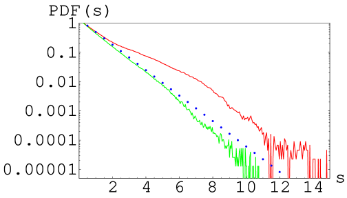
Refer to caption
Figure 1: One-mode amplitude PDF’s at two wavenumbers: upper curve at $k_{1}$ and the lower curve at and $k_{2}$ such that $k_{1}>k_{2}$. Dashed line corresponds to the Rayleigh distribution.

This figure shows that at a high $k$ the PDF tail is depleted with respect to the Rayleigh distribution, whereas at a lower $k$ it is enhanced which corresponds to intermittency at this scale. Similar conclusion that the gravity wave turbulence is intermittent at low rather than high wavenumbers was reached on the basis of numerical simulations in [33]. To understand the flux reversal leading to intermittency appears in the one-mode statistics, one has to consider fluxes in the multi-mode phase space which will be done in the next section.

12 Intermittency and the multi-mode probability vortex.

In the previous section, we established that one-mode PDF’s can deviate from the Rayleigh distributions if the flux of probability in the amplitude space is not equal to zero. However, in the full $N$-mode amplitude space, the flux lines cannot originate or terminate, i.e. there the probability “sources” and “sinks” are impossible, see (69). Even adding forcing or dissipation into the dynamical equations does not change this fact because this can only modify the expression for the flux (see the Appendix) but it cannot change the PDF continuity equation (65). Thus, presence of the finite flux for the one-point PDF’s corresponds to deviation of the flux lines from the straight lines in the $N$-mode amplitude space. The global structure of such a solution in the $N$-mode space corresponds to a $N$ dimensional probability vortex. This probability vortex is illustrated in figure ? which sketches its projection onto a a 2D plane corresponding to one low-wavenumber and one high-wavenumber amplitudes. Taking 1D sections of this vortex one observes a positive one-mode flux at high $k$ and a negative one-mode flux at low $k$, in accordance with the numerical observations of figure 2.

Refer to caption
Figure 2: Projection of the probability flux vortex on a $(s_{1},s_{2})$ plane where $s_{1}$ and $s_{2}$ are the amplitudes at wavenumbers $k_{1}$ and $k_{2}$ such that $k_{1}>k_{2}$.

We should say, however, that existence of the probability vortex solutions, although consistent with numerics, remains hypothetical and further work needs to be done to find solutions of (69) with non-zero curl.

13 Discussion.

In this paper, we reviewed recent work in the field of Wave Turbulence devoted to study non-Gaussian aspects of the wave statistics, intermittency, validation of the phase and amplitude randomness, higher spectral moments and fluctuations. We also presented some new results, particularly derivation of the analog of the Peierls-Brout-Prigogine equation for the four-wave systems. The wavefileds we dealt with are, generally, characterised by non-decaying correlations along certain directions in the coordinate space. These fields are typical for WT because, due to weak nonlinearity, wavepackets preserve identity over long distances. One of the most common examples of such long-correlated fields is given by the typical initial condition in numerical simulations where the phases are random but the amplitudes are chosen to be deterministic. We showed that wavefields can develop enhanced probabilities of high amplitudes at some wavenumbers which corresponds to intermittency. Simultaneously, at other wavenumbers, the probability of high amplitudes can be depleted with respect to Gaussian statistics. We showed that both PDF tail enhancement and its depletion related to presence of a probability flux in the amplitude space (which is positive for depletion and negative for the enhancement). We speculated that the $N$-dimensional space of $N$ amplitudes, these fluxes correspond to an $N$-dimensional probability vortex. We argued that presence of such vortex is prompted by non-existence of a zero-amplitude-flux solution corresponding to the KZ spectrum with de-correlated amplitudes. Finding such a probability vortex solution analytically remains a task for future.

14 Appendix: Wave Turbulence with sources and sinks

One of the central discoveries in Wave Turbulence was the power-law Kolmogorov-Zakharov (KZ) spectrum, $n^{kz}\sim k^{\nu}$, which realise themselves in presence of the energy sources and sinks separated by a large inertial range of scales. The exponent $\nu$ depends on the scaling properties of the interaction coefficient and the frequency. Most of the previous WT literature is devoted to study of KZ spectra and a good review of these works can be found in [1]. We are not going review these studies here, but instead we are going to find out how adding such energy sources and sinks will this modify the evolution equations for the statistics. Instead of the Hamiltonian equation (1) let us consider

$\displaystyle i\dot{c}_{l}$ $\displaystyle=$ $\displaystyle\frac{\partial{\cal H}}{\partial\bar{c}_{l}}+i\tilde{\gamma}_{l}c_{l},$ (98)

where $\tilde{\gamma}_{l}$ describes sources and sinks of the energy, e.g. due to instability and viscosity respectively. Easy to see that this linear term will not change the structure of the $N$-mode PDF equation (65) but it will lead to re-definition of the flux:

$${\cal F}_{j}\to{\cal F}_{j}-\tilde{\gamma}_{j}s_{j}P.$$ (99)

In the one-mode equations, this simply means renormalisation

$$\gamma\to\gamma-\tilde{\gamma}.$$ (100)

Thus we arrive at a simple message that the energy sources and sinks do not produce any “sources” or “sinks” for the flux of probability.

In the inertial range, there is no flux modification and one can easily find $F=0$ solution of (90) for the one-mode PDF,

$$P^{(a)}_{j}=(1/n_{j}^{kz})\exp(-s_{j}/n_{j}^{kz}),$$ (101)

where $n_{j}^{kz}$ is the KZ spectrum (solving the kinetic equation in the inertial range). However, it is easy to check by substitution that the product of such one-mode PDF’s, ${\cal P}=\Pi_{j}(1/n_{j}^{kz})\exp(-s_{j}/n_{j}^{kz})$, is not an exact solution to the multi-mode equation (65). Thus, there have to be corrections to this expression related either to a finite flux, an amplitude correlation or both.

References

  • [1] V.E. Zakharov, V.S. L’vov and G.Falkovich, ”Kolmogorov Spectra of Turbulence”, Springer-Verlag, 1992.
  • [2] D.J. Benney and P.Saffman, Proc Royal. Soc, A(1966), 289, 301-320; B. J . Benney and A.C. Newell, Studies in Appl. Math. 48 (1) 29 (1969).
  • [3] A.A. Galeev and R.Z. Sagdeev, in “Reviews of Plasma Physics” Vol. 6 (Ed. M A Leontovich) (New York: Consultants Bureau, 1973)
  • [4] A.C. Newell: Rev. Geophys. 6, 1 (1968)
  • [5] V.E. Zakharov, N.N. Filonenko, Weak turbulence of capillary waves, Zh. Prikl. Mekh. Tekh. Fiz. 4 (5) 62-67 (1967) [J. Appl. Mech. Tech. Phys. 4, 506-515 (1967)]; V.E. Zakharov, N.N. Filonenko, The energy spectrum for stochastic oscillations of a fluid surface, Doclady Akad. Nauk SSSR 170, 1292-1295 (1966) [Sov. Phys. Docl. 11, 881-884 (1967)].
  • [6] K. Hasselmann, “Freely decaying weak turbulence for sea surface gravity waves”, J. Fluid Mech 12 481 (1962).
  • [7] S. Dyachenko, A.C. Newell, A. Pushkarev, V.E. Zakharov: Physica D 57, 96 (1992)
  • [8] H.W. Wyld, Ann. Phys. 14 (1961) 143.
  • [9] V.E. Zakharov, V.S. L’vov, The statistical description of the nonlinear wave fields, Izv. Vuzov, Radiofizika 18 (10) 1470-1487 (1975).
  • [10] V.S. Lvov, Y.V. Lvov, A.C. Newell and V.E. Zakharov, “Statistical description of acoustic turbulence” Phys. Rev. E 56 (1997) 390.
  • [11] R.C. Davidson “Methods in Nonlinear Plasma Theory”, New York: Academic Press 1972.
  • [12] A.N. Pushkarev, V.E. Zakharov, “Turbulence of capillary waves” PRL 76, 3320-3, (1996). Physica D, 135, 98, (2000).
  • [13] V.E. Zakharov and L.I. Piterbarg, Canonical variables for Rossby waves and plasma drift waves, Phys. Lett. A, 126 (1988), No. 8-9, 497-500.
  • [14] A.M.Balk and S.V. Nazarenko “On the Physical Realisability of Anisotropic Kolmogorov Spectra of Weak Turbulence” Sov.Phys.-JETP 70 (1990) 1031.
  • [15] V.E. Zakharov, S.L. Musher, A.M. Rubenchik: Phys. Rep. 129, 285 (1985)
  • [16] S. Galtier, S.V. Nazarenko, A.C. Newell and A. Pouquet A weak turbulence theory for incompressible MHD, Journal of Plasma Phys., 63 (2000) 447-488.
  • [17] V. P. Krasitskii, On reduced equations in the Hamiltonian theory of weakly nonlinear surface-waves, J. Fluid Mech. 272: 1-20 (1994).
  • [18] Yu. V. Lvov and E.G. Tabak, PRL 87, 168501, (2001); Y.V. Lvov, K.L. Polzin and E.G.Tabak, PRL, 92, 128501 (2004).
  • [19] R. Peierls, Annalen Physik 3 (1029) 1055.
  • [20] R. Brout and I. Prigogine, Physica 22 (1956) 621-636.
  • [21] G.M. Zaslavskii and R.Z. Sagdeev, Sov.Phys. JETP 25 (1967) 718.
  • [22] Yu. Lvov and Sergey Nazarenko, “Noisy” spectra, long correlations and intermittency in wave turbulence, Phys. Rev. E 69, 066608 (2004) (2004). Also at http://arxiv.org/abs/math-ph/0305028.
  • [23] Y. Choi, Yu. Lvov, S.V. Nazarenko and B.Pokorni, Anomalous probability of high amplitudes in wave turbulence, submitted to PRL. Also at http://arxiv.org/abs/math-ph/0404022
  • [24] Y. Choi, Yu. Lvov and S.V. Nazarenko, Probability densities and preservation of randomness in wave turbulence, accepted to Phys Lett A; Y. Choi, Yu. Lvov and S.V. Nazarenko, Joint statistics of amplitudes and phases in Wave Turbulence, submitted to Physica D;
  • [25] V.E. Zakharov and E. Shulman, in: What is integrability? (Ed. by Zakharov) Springer-Verlag 1991, p 190.
  • [26] V.E. Zakharov, P. Guyenne, A.N. Pushkarev, F. Dias, Wave turbulence in one-dimensional models, Physica D 152-153 573-619 (2001)
  • [27] R. Micha and I. Tkachev, Turbulent Thermalization, arXiv:hep-ph/0403101.
  • [28] A.C. Newell and V.E. Zakharov, “Rough sea foam”, PRL 69, 1149 (1992).
  • [29] M. Onorato et al, PRL 89, 144501, (2002).
  • [30] P.A.E.M. Janssen, “Nonlinear four-wave interactions and freak waves” J. Phys Oceanography, 33 864 (2003).
  • [31] C. Connaughton S. Nazarenko and A.C. Newell, Physica D, 184 86-97 (2003)
  • [32] L. Biven, S.V. Nazarenko and A.C. Newell, ”Breakdown of wave turbulence and the onset of intermittency”, Phys Lett A, 280, 28-32, (2001); A.C. Newell, S.V. Nazarenko and L. Biven, Physica D, 152-153, 520-550, (2001).
  • [33] N. Yokoyama, J. Fluid Mech. 501 (2004), 169-178.