The Linear Boltzmann Equation as the Low Density Limit of a Random Schrödinger Equation

Abstract

We study the long time evolution of a quantum particle interacting with a random potential in the Boltzmann-Grad low density limit. We prove that the phase space density of the quantum evolution defined through the Husimi function converges weakly to a linear Boltzmann equation. The Boltzmann collision kernel is given by the full quantum scattering cross section of the obstacle potential.

1 The Model and the Result

The Schrödinger equation with a random potential describes the propagation of quantum particles in an environment with random impurities. In the first approximation one neglects the interaction between the particles and the problem reduces to a one-body Schrödinger equation. With high concentration of impurities the particle is localized, in particular no conduction occurs [1, 2, 3, 8, 11, 12]. In the low concentration regime conduction is expected to occur but there are no rigorous mathematical proof of the existence of the extended states except for the Bethe lattice [16, 17]. In this paper we study the long time evolution in the low concentration regime in a specific scaling limit, called the low density or Boltzmann-Grad limit. Our model is the quantum analogue of the low density Lorentz gas. As the time increases, the concentration will be scaled down in such a way that the total interaction between the particle and the obstacles remains bounded for a typical configuration. Therefore our result is far from the extended states regime which requires to understand the behavior of the Schrödinger evolution for arbitrary long time, independently of the fixed (low) concentration of impurities. We start by defining our model and stating the main result.

Let $\Lambda_{L}\subset\mathbb{R}^{d}$ be a cube of width $L$ and let $V_{0}(x)$ be a smooth radial function with a sufficiently strong decay to be specified later. Denote by $\omega=(x_{\alpha}),\alpha=1,\ldots,N$, the configuration of uniformly distributed obstacles and let

$$\varrho:=\frac{N}{L^{d}}$$ (1.1)

be the density of the obstacles. We are interested in the evolution of a quantum particle in the random environment generated by these obstacles. The Schrödinger equation governing the quantum particle is given by:

$$i\partial_{t}\psi_{t}=H_{N,L}\psi_{t}\,,\,\,\,\psi_{t=0}=\psi_{0}\;,$$ (1.2)

where the Hamiltonian is given by:

$$H_{N,L}=H:=-\frac{1}{2}\Delta+V_{\omega},\,\,\qquad V_{\omega}=\sum\limits_{\alpha=1}^{N}V_{\alpha},\,\,\,V_{\alpha}(x):=V_{0}(x-x_{\alpha})\;$$ (1.3)

with periodic boundary conditions on $\Lambda_{L}$. We have used lower case letters, $(x,t)$, to denote the space and time variables in the microscopic (atomic) scale.

We shall always take first the simultaneous $L\to\infty$, $N\to\infty$ limits, with a fixed density, $\varrho=N/L^{d}$, before any other limit. The finite box $\Lambda_{L}$ is just a technical device to avoid infinite summation in the potential term. Our method works for any dimension $d\geq 3$, but we restrict ourselves here to the case $d=3$.

As a first step toward a study of conduction, one considers certain scaling limits. Let $\varepsilon$ be the scale separation parameter between microscopic and macroscopic variables. In reality, $\varepsilon=1\AA/1\;\mathrm{cm}=10^{-8}$; here we always take the idealized $\varepsilon\to 0$ limit. Define the macroscopic coordinates $(X,T)$ by

$$(X,T):=(x\varepsilon,t\varepsilon)\;.$$

Note that the velocity is not rescaled, $\frac{X}{T}=\frac{x}{t}$. In this paper we will treat the following scaling limit problem:

$\bf{Low\,density\,limit\,(L.D.L.):}$ Let $\varrho=\varepsilon\varrho_{0}$ for some fixed positive density $\varrho_{0}$:

$$i\partial_{t}\psi_{\omega,t}^{\varepsilon}=\Big{[}-\frac{1}{2}\Delta+\sum\limits_{\alpha=1}^{N}V_{{\alpha}}(x)\Big{]}\psi_{\omega,t}^{\varepsilon}\,.$$ (1.4)

Another interesting scaling limit which has been studied in the literature is:

$\bf{Weak\,coupling\,limit\,(W.C.L.):}$ Fix the density $\varrho=\varrho_{0}$ and scale the strength of the external potential by $\sqrt{\varepsilon}$:

$$i\partial_{t}\psi_{\omega,t}^{\varepsilon}=\Big{[}-\frac{1}{2}\Delta+\sqrt{\varepsilon}\sum\limits_{\alpha=1}^{N}V_{{\alpha}}(x)\Big{]}\psi_{\omega,t}^{\varepsilon}\;.$$ (1.5)

In a related model, the random obstacle potential $\sum_{\alpha}V_{\alpha}$ is replaced with a Gaussian field $V_{\omega}(x)$ with a decaying, $\varepsilon$-independent covariance.

It turns out that in both the L.D.L and W.C.L. models these are the weakest interaction strengths that result in a nontrivial (non-free) macroscopic evolution in the scaling limit $\varepsilon\to 0$.

The Wigner transform of a wave function $\psi$ is defined by:

$$W_{\psi}(x,v):=\int_{\mathbb{R}^{3}}\overline{\psi\Big{(}x+\frac{z}{2}\Big{)}}\psi\Big{(}x-\frac{z}{2}\Big{)}e^{ivz}dz\;.$$ (1.6)

The Wigner transform typically has no definite sign but the associated Husimi function is nonnegative at appropriate scales. The Husimi function at scale $(\ell_{1},\ell_{2})$ is defined by:

$$H_{\psi}^{\ell_{1},\ell_{2}}:=W_{\psi}*_{x}G^{\ell_{1}/\sqrt{2}}*_{v}G^{\ell_{2}/\sqrt{2}}\;,$$

where $G^{\delta}$ is the standard Gaussian with variance $\delta^{2}$, i.e.,

$$G^{\delta}(z):=(2\pi\delta^{2})^{-\frac{3}{2}}e^{-\frac{z^{2}}{2\delta^{2}}}\;.$$ (1.7)

The Husimi function at scale $\ell_{1}=\ell$, $\ell_{2}=\ell^{-1}$ is the coherent state at scale $\ell$ defined by

$$H_{\psi}^{\ell,\ell^{-1}}(x,v)=C_{\psi,\ell}(x,v):=\langle\psi,\pi_{x,v}^{\ell}\psi\rangle\;,$$

where $\pi_{x,v}^{\ell}$ is the projection onto the $L^{2}$ normalized state $G^{\ell}(x-z)e^{izv}$. Clearly $C_{\psi,\ell}$ is positive and

$$\int C_{\psi,\ell}(x,v)dxdv=\|\psi\|_{2}^{2}=1\;.$$ (1.8)

Thus $C_{\psi,\ell}$ can be considered as a probability density on the phase space at atomic scale. The accuracy for the space variable in the coherent state $C_{\psi,\ell}$ is of order $\ell$, and the accuracy is of order $\ell^{-1}$ for the velocity variable. This is optimal by the uncertainty principle. Unfortunately we cannot keep this accuracy along our proof, and we need a small extra smoothing.

The basic object we shall study is the Husimi function on scale $\ell_{1}=\varepsilon^{-1+\mu}$, $\ell_{2}=\varepsilon^{\mu}$ with some $0<\mu<1/2$, which can also be written as

$$H_{\psi}^{\varepsilon^{-1+\mu},\varepsilon^{\mu}}=H_{\psi}^{\varepsilon^{-\mu},\varepsilon^{\mu}}\ast_{x}G^{\ell(\varepsilon)/\sqrt{2}}=C_{\psi,\varepsilon^{-\mu}}\ast_{x}G^{\ell(\varepsilon)/\sqrt{2}}\;,$$ (1.9)

where $\ell(\varepsilon)=\varepsilon^{\mu}\sqrt{\varepsilon^{-2}-\varepsilon^{-4\eta}}$. We can rescale it to the macroscopic scale by defining

$$H^{(\varepsilon,\mu)}_{\psi}(X,V):=\varepsilon^{-3}H_{\psi}^{\varepsilon^{-1+\mu},\varepsilon^{\mu}}(X/\varepsilon,V)\geq 0\;.$$ (1.10)

From (1.8), (1.9) and (1.10) it follows that $H^{(\varepsilon,\mu)}_{\psi}(X,V)$ defines a probability density on the macroscopic phase space $\mathbb{R}^{6}$.

Notice that the velocity in $H^{(\varepsilon,\mu)}_{\psi}$ is not rescaled. The accuracy for both the (macroscopic) space and velocity variables in $H^{(\varepsilon,\mu)}_{\psi}$ is now of order $\varepsilon^{\mu}$. We shall use this nonnegative phase space density function to represent the true quantum mechanical function $\psi$. Our goal is to prove that the macroscopic phase space density of $\psi^{\varepsilon}_{t}$ converges to a solution of the linear Boltzmann equation as in the classical case, except that the classical differential scattering cross section is replaced by the quantum differential scattering cross section.

We now recall the linear Boltzmann equation for a time dependent phase space density $F_{T}(X,V)$ with collision kernel $\Sigma(U,V)$:

$$\partial_{T} F_{T}(X,V)+V\cdot\nabla_{X}F_{T}(X,V)$$

$$= \int\Big{[}\Sigma(U,V)F_{T}(X,U)-\Sigma(V,U)F_{T}(X,V)\Big{]}dU$$

$$= \int\Sigma(U,V)F_{T}(X,U)dU-\Sigma F_{T}(X,V)\;,$$ (1.11)

where $\Sigma:=\int\Sigma(V,U)dU$ is the total cross section. In our setting $\Sigma(V,U)$ will be defined later on in the Main Theorem.

For any function $f$ on $\mathbb{R}^{3}$ we introduce the norms

$$\|f\|_{M,N}:=\|\langle x\rangle^{M}\langle\nabla\rangle^{N}f\|_{2},\qquad N,M\in\mathbb{N}\;,$$

where $\langle x\rangle:=(1+x^{2})^{1/2}$.

Suppose $V_{0}$ is a smooth, decaying and radially symmetric potential such that

$$\lambda_{0}:=\|V_{0}\|_{50,50}$$ (1.12)

is sufficiently small. In particular, the one body Hamiltonian $H_{1}:=-\frac{1}{2}\Delta+V_{0}$ has no bound states and asymptotic completeness holds, i.e. both the incoming and outgoing Hilbert spaces are the full space $L^{2}(\mathbb{R}^{3})$. Recall the wave operators $\Omega_{\mp}=\lim_{s\to\infty}e^{\pm isH_{0}}e^{\mp isH_{1}}$, where $H_{0}:=-\frac{1}{2}\Delta$. The kernel of the scattering operator $S=\Omega^{\ast}_{-}\Omega_{+}$ in the Fourier space exists and can be written as

$$S(u,v)=\delta(u-v)-2\pi i\delta(u^{2}-v^{2})T_{\mathrm{scat}}(u,v).$$

The differential scattering cross section can be defined as

$$\sigma(u,v):=4\pi\,\underbrace{\delta(u^{2}-v^{2})}_{\hbox{ on-shell}}|T_{\mathrm{scat}}(u,v)|^{2}.$$ (1.13)

We shall choose initial data of the form

$$\psi_{0}^{\varepsilon}(x)=\varepsilon^{3/2}h(\varepsilon x)e^{iu_{0}\cdot x}\;,$$

where $u_{0}\in\mathbb{R}^{3}$, $\|h\|_{30,30}<\infty$ and $h$ is $L^{2}$-normalized. This implies $\|\widehat{\psi}_{0}^{\varepsilon}\|_{30,0}<\infty$ .

We will usually drop the ”hat” on the initial wave function as we will be working in momentum space. It should be noted that the specific form of our initial wave function is used only in the last step - in the identification of the limit. Our result certainly holds for a general class of initial conditions which satisfy $\|\widehat{\psi}_{0}^{\varepsilon}\|_{30,0}<\infty$ and that have a limiting macroscopic phase space density.

It is straightforward to check that the rescaled Husimi functions (1.10) of the initial data converge weakly as probability measures on $\mathbb{R}^{6}$ as $\varepsilon\to 0$, i.e.

$$H^{(\varepsilon,\mu)}_{\psi^{\varepsilon}_{0}}(X,V)dXdV\to|h(X)|^{2}\delta(V-u_{0})dXdV\;.$$

We define

$$F_{0}(X,V):=|h(X)|^{2}\delta(V-u_{0})$$

to be the initial data of the limiting Boltzmann equation. We can now state our theorem concerning the low density limit:

Main Theorem.

Suppose $d=3$ and let $\mu>0$ be sufficiently small. Suppose the random environment $\omega$ is uniformly distributed with density $\varrho=\varrho_{0}\varepsilon$ with some fixed $\varrho_{0}>0$. Let $V_{0}$ be a radially symmetric potential such that $\lambda_{0}:=\|V_{0}\|_{50,50}$ is sufficiently small. Let $\psi_{\omega,t}^{\varepsilon}$ be the solution to the Schrödinger equation (1.4) with $L^{2}$-normalized initial data $\psi^{\varepsilon}_{0}$ of the following form

$$\psi^{\varepsilon}_{0}(x)=\varepsilon^{3/2}h(\varepsilon x)e^{iu_{0}\cdot x}$$

where $\|h\|_{30,30}<\infty$, $\|h\|_{2}=1$. Then for any $T>0$, and any bounded, continuous test function $J$,

$$\lim_{\varepsilon\to 0}\lim_{L\to\infty}\Big{|}\int dXdVJ(X,V)\,\Big{[}{\mathbf{E}}H^{(\varepsilon,\mu)}_{\psi_{\omega,T/\varepsilon}^{\varepsilon}}(X,V)-F_{T}(X,V)\Big{]}\Big{|}=0\,,$$

where $F_{T}(X,V)$ satisfies the linear Boltzmann equation (1.11) with initial data given by $F_{0}(X,V)=|h(X)|^{2}\delta(V-u_{0})$ and with effective collision kernel $\Sigma(U,V)=\varrho_{0}\,\sigma(U,V)$. Here $\sigma(U,V)$ is the differential scattering cross section given in (1.13).

Our result holds for a larger class of distributions of obstacles, but for simplicity we assume the uniform distribution in this paper.

The analogous result in the W.C.L. model was proven by H. Spohn [20] in the case where the obstacles are distributed according to a Gaussian law and macroscopic time is small, $T\leq T_{0}$. His result was extended to higher order correlation functions by Ho-Landau-Wilkins [14] under the same assumptions. The W.C.L. model with a Gaussian field was proven globally in time by Erdős and Yau in [9]. Later the method was extended to general distributions by Chen in [5]. Chen also showed [6] that the convergence of the expected Wigner transform to the Boltzmann equation holds in $L^{r}$ for $r\geq 1$.

The present proof is similar in spirit to the W.C.L. proof in [9]. The main difference between the two models and proofs lies in the Boltzmann collision kernel, $\Sigma$. In the L.D.L. model, $\Sigma$ involves summing up the complete Born series of each individual obstacle scattering in contrast to the W.C.L. model, where only the first Born approximation is needed. Unlike in the W.C.L. model, in the low density environment once the quantum particle is in the neighborhood of an obstacle, it can collide with it many times with a non-vanishing amplitude. Moreover, if two obstacles are near to each other, then complicated double recollision patterns arise with comparable amplitudes. On a technical level, this difference forced us to completely reorganize the diagrammatic expasion of [9]. Most importantly, the recollision diagrams have bigger amplitude in the L.D.L model and their estimate required several new ideas.

The classical analogue of the L.D.L. model is the classical Lorentz gas. It is proved by G. Gallavotti [13], H. Spohn [21], and Boldrighini, Bunimovich and Sinai [4] that the evolution of the phase space density of a classical Lorentz gas converges to a linear Boltzmann equation. However, the classical W.C.L. behavior is governed by a Brownian motion instead of the Boltzmann equation - see Kesten and Papanicolaou [15] and Dürr, Goldstein and Lebowitz [7].

In principle, one is interested in the behavior of $T\to H^{(\varepsilon,\mu)}_{\psi_{\omega,T/\varepsilon}^{\varepsilon}}$ as a process for typical $\omega$. This means one has to consider the joint distributions of $(H^{(\varepsilon,\mu)}_{\psi_{\omega,T_{1}/\varepsilon}^{\varepsilon}},\cdots,H^{(\varepsilon,\mu)}_{\psi_{\omega,T_{n}/\varepsilon}^{\varepsilon}})$. We believe that there is no intrinsic difficulty to extend our method to this setting. But the proof will certainly be much more involved.

2 Preliminaries

2.1 Notation

For convenience, we fix a convention to avoid problems with factors of $2\pi$ arising from the Fourier transform. We define $dx$ to be the Lebesgue measure on $\mathbb{R}^{3}$ divided by $(2\pi)^{-3/2}$; i.e.,

$$\int dx=\frac{1}{(2\pi)^{3/2}}\int_{\mathbb{R}^{3}}d^{*}x,$$

where we reserve the notation $d^{*}x$ for the genuine $3$-dimensional Lebesgue measure. This convention will apply to any space or momentum variable in $3$ dimensions but $\it{not}$ to one-dimensional integration (like time variables and their variables), where integration will be the standard, unscaled, Lebesgue measure on the line. With this convention, the three dimensional Fourier transform (which will be usually denoted by a hat) is:

$$\widehat{f}(p)=\mathcal{F}f(p):=\int f(x)e^{-ipx}dx$$

and its inverse:

$$f(x)=\mathcal{F}^{-1}\widehat{f}(x)=\int\widehat{f}(p)e^{ipx}dp\;.$$

Wave functions will always be represented in momentum space, $\psi(p)$, hence we can omit the hat from their notation.

The other convention is related to the fact that we will be considering the problem on the torus $\Lambda:=L\mathbb{T}^{3}$ where $\mathbb{T}^{3}$ is the unit torus. Correspondingly, all the momenta in this paper will be on the discrete lattice $(\mathbb{Z}/L)^{3}$. The momentum variables will be denoted by letters $p,q,r,u,v$ or $w$. The delta function is defined as:

$$\delta(p) :=|\Lambda|\text{ for $p=0$}$$

$$\delta(p) :=0\text{ for $p\in(\mathbb{Z}/L)^{3}\setminus\{0\}$ .}$$ (2.1)

Nevertheless we will use the continuous formalism, under the identification

$$\int dp:=\frac{1}{(2\pi)^{\frac{3}{2}}|\Lambda|}\sum\limits_{p\in(\mathbb{Z}\setminus L)^{3}}\;.$$ (2.2)

Again, this will only apply to momenta variables. The delta functions with time variables will remain the usual continuous delta functions. The convention (2.2) should not cause any confusion, as $L\to\infty$ can be taken at any stage of the proof independently of all other limits.

Gothic script will be used to denote a set of variables, in particular, momenta. Define:

$${\mathfrak{p}}_{m_{1},m_{2}}:= \{p_{j}\}_{j=m_{1}}^{m_{2}}=(p_{m_{1}},p_{m_{1}+1},\ldots,p_{m_{2}})$$

$${\mathfrak{p}}_{m}:= {\mathfrak{p}}_{1,m}.$$ (2.3)

In some instances, we will need to single out the first momenta and write $(p_{0},{\mathfrak{p}}_{m})$ instead of ${\mathfrak{p}}_{0,m}$. Similar convention applies to other momentum variables. Moreover, for any $\mathfrak{l}_{0,b}:=(\ell_{0},\ldots,\ell_{b})$, where $\ell_{j}$ are non-negative integers for $j=0,\ldots,b$, we define

$${\mathfrak{p}}_{0,b}^{\mathfrak{l}_{0,b}}:=(\underbrace{p_{0},\ldots,p_{0}}_{\ell_{0}+1},\ldots,\underbrace{p_{b},\ldots,p_{b}}_{\ell_{b}+1}).$$ (2.4)

If $\operatorname{Log}x$ is the standard natural logarithm function (on the positive line), define for $x>0$:

$$\log x:=\begin{cases}1&\text{for $x\leq e$}\\ \operatorname{Log}x&\text{for $x>e$ .}\end{cases}$$ (2.5)

If $x\geq 1$, we define $x^{\operatorname{O}(1)}$ to be $x^{k}$ for some positive constant $k$ which is independent of any parameter (such as $\varepsilon$).

Finally, if $A,B$ are fully ordered sets, unordered set operations will be denoted by their usual notation (e.g. $\cup,\cap,\in$, etc.). Define $A\oplus B$ to be the concatenation of $A$ and $B$, i.e., the ordered set where the ordering of $A$ supersedes that of $B$. We will at times write $AB:=A\oplus B$. $A\prec B$ will denote ordered inclusion, i.e. $A\subset B$ and the ordering coincides.

2.2 The Duhamel Formula

For any fixed $n_{0}\geq 1$, the Duhamel formula states:

$$e^{-itH}= \sum_{m=0}^{n_{0}-1}(-i)^{m}\int_{0}^{t*}\left[ds_{j}\right]_{0}^{m}e^{-is_{0}H_{0}}V_{\omega}e^{-is_{1}H_{0}}V_{\omega}\cdots V_{\omega}e^{-is_{m}H_{0}}$$

$$+(-i)^{n_{0}}\int_{0}^{t*}\left[ds_{j}\right]_{0}^{n_{0}}e^{-is_{0}H}V_{\omega}e^{-is_{1}H_{0}}V_{\omega}\cdots V_{\omega}e^{-is_{n_{0}}H_{0}}\;,$$ (2.6)

where $H$ is the (full) Hamiltonian given in (1.3) and:

$$\int_{0}^{t*}\left[ds_{j}\right]_{m}^{n}:=\int_{0}^{t}\ldots\int_{0}^{t}\Big{(}\prod_{j=m}^{n}ds_{j}\Big{)}\,\delta\Big{(}t-\sum_{j=m}^{n}s_{j}\Big{)}\;,$$ (2.7)

where $m\leq n$, and the star refers to the constraint $t=\sum s_{j}$. $V_{\omega}$ is the potential given in (1.3) and $H_{0}=-\frac{1}{2}\Delta$. Expanding the potential $V_{\omega}=\sum_{{\alpha}=1}^{N}V_{\alpha}$ in the Duhamel formula, we generate many terms. We can label these terms by a sequence of obstacles, say, ${\boldsymbol{\alpha}}=({\alpha}_{1},{\alpha}_{2},\cdots,{\alpha}_{n})$. The terms without $e^{-itH}$ (in the first line of (2.6)) will be called fully expanded, the others will be called truncated.

We write the Duhamel formula in momentum space. The kernel of the typical fully expanded term is of the form:

$$\int_{0}^{t*}\left[ds_{j}\right]_{0}^{n}e^{-is_{0}p_{0}^{2}/2}\hat{V}_{{\alpha}_{1}}(p_{0}-p_{1})e^{-is_{1}p_{1}^{2}/2}\hat{V}_{{\alpha}_{2}}(p_{1}-p_{2})\cdots e^{-is_{n}p_{n}^{2}/2}$$ (2.8)

with the intermediate momenta $p_{1},p_{2},\ldots,p_{n-1}$ integrated out. The truncated terms are of the same form with $e^{-is_{0}p_{0}^{2}/2}$ replaced with $e^{-is_{0}H}$:

$$\int_{0}^{t*}\left[ds_{j}\right]_{0}^{n}e^{-is_{0}H}\hat{V}_{{\alpha}_{1}}(\cdot-p_{1})e^{-is_{1}p_{1}^{2}/2}\hat{V}_{{\alpha}_{2}}(p_{1}-p_{2})\cdots e^{-is_{n}p_{n}^{2}/2}.$$ (2.9)

The obstacles in ${\boldsymbol{\alpha}}=({\alpha}_{1},{\alpha}_{2},\ldots,{\alpha}_{n})$ are allowed to repeat. We can relabel them by a sequence of centers

$$A:=({\alpha}_{1},{\alpha}_{2},\ldots,{\alpha}_{m}),\quad x_{{\alpha}_{j}}\in\omega\hbox{ for all }j$$

and a sequence of non-negative numbers

$$(k_{1},k_{2},\ldots,k_{m})\;,$$

where $k_{j}+1$ denotes the number of times ${\alpha}_{j}$ repeats itself consecutively (we say that $k_{j}$ is the number of internal recollisions). The sequence $A$ has the property that ${\alpha}_{j}\neq{\alpha}_{j+1}$. In order words, the original collision sequence is given by

$$(\underbrace{{\alpha}_{1},\ldots,{\alpha}_{1}}_{k_{1}+1},\underbrace{{\alpha}_{2},\ldots,{\alpha}_{2}}_{k_{2}+1},\ldots,\underbrace{{\alpha}_{m},\ldots,{\alpha}_{m}}_{k_{m}+1})\;.$$ (2.10)

We shall divide the set of momenta into internal ones and external ones. The internal momenta are running between the same obstacles; the external ones are the rest. The internal momenta will be integrated out first (resummation of loop diagrams). Hence repeated consecutive collisions with the same obstacle, internal collisions, will be considered as a single (physical) collision and will be referred to as a collision with a center. When we speak of the number of collisions, we will actually be referring to the number of collisions with centers. For example, in the sequence (2.10) there are $\sum_{j=1}^{m}(k_{j}+1)$ collisions, $m$ centers and there are $k_{j}$ internal momenta running among the $k_{j}+1$ collisions with the same center $\alpha_{j}$.

Collision histories will be recorded with the ordered set $A$. Typically we will use the variable $m$ to denote the cardinality of $A$, $m=|A|$. Next, let $J$ be a set of lexicographically ordered double indices for the internal momenta

$$J=J_{m,{\mathbf{k}}}:=\Bigl{(}11,12,\ldots,1k_{1},21,22,\ldots 2k_{2},\ldots mk_{m}\Bigr{)}\;,$$ (2.11)

where ${\mathbf{k}}=(k_{1},k_{2},\ldots,k_{m})$ denotes the number of the internal momenta for the obstacle ${\alpha}_{j}$. We shall denote the internal momenta by ${\mathfrak{q}}_{J}:=(q_{j\ell})_{j\ell\in J_{m,{\mathbf{k}}}}$.

Since $\widehat{V}_{{\alpha}}:=\mathcal{F}V_{{\alpha}}=e^{-ipx_{\alpha}}\widehat{V}(p)$, we are able to separate the random part of the potential, in the form of a random phase, from the deterministic part. Consequently, denote the random phase corresponding to collision history $A$ by

$$\chi(A;{\mathfrak{p}}_{0,m}):=\prod_{j=1}^{m}e^{-ix_{\alpha_{j}}(p_{j-1}-p_{j})}.$$ (2.12)

Note that it is independent of the internal momenta. Then the deterministic part of the potentials is given by

$$L({\mathfrak{p}}_{0,m},{\mathfrak{q}}_{J_{m,{\mathbf{k}}}}):=\prod_{j=1}^{m}\hat{V}_{0}(p_{j-1}-q_{j1})\hat{V}_{0}(q_{j1}-q_{j2})\ldots\hat{V}_{0}(q_{jk_{j}}-p_{j}).$$ (2.13)

In the case where $k_{j}=0$, we only have the term: $\hat{V}_{0}(p_{j-1}-p_{j})$. Notice that this expression is independent of the location of the obstacles; that information is contained in the random phase, $\chi$.

Given a set of momenta, ${\mathfrak{r}}_{0,m}$, define the free evolution kernel as:

$$K(t;r_{0},{\mathfrak{r}}_{m}):=(-i)^{m}\int_{0}^{t*}\left[ds_{j}\right]_{j=0}^{m}\prod_{j=0}^{m}e^{-is_{j}r_{j}^{2}/2}.$$ (2.14)

Notice that this expression is independent of the order of the momenta. Considering (2.8) and using the previously established notation for internal and external momenta, the free evolution kernel associated with the collision sequence $A$ and internal momenta ${\mathbf{k}}$ is:

$$K(t;{\mathfrak{p}}_{0,m},{\mathfrak{q}}_{J_{m,{\mathbf{k}}}}):= K(t;p_{0},q_{11},\ldots,q_{1k_{1}},p_{1},q_{21},\ldots,p_{m-1},q_{m1},\ldots,q_{mk_{m}},p_{m}).$$

Define the fully summed (for internal collisions) free evolution kernel as:

$${\mathcal{K}}(t;{\mathfrak{p}}_{0,m}):=\sum_{k_{1},\ldots,k_{m}=0}^{\infty}\int d{\mathfrak{q}}_{J_{m,{\mathbf{k}}}}K(t;p_{0},{\mathfrak{p}}_{m},{\mathfrak{q}}_{J_{m,{\mathbf{k}}}})L(p_{0},{\mathfrak{p}}_{m},{\mathfrak{q}}_{J_{m,{\mathbf{k}}}}).$$ (2.15)

With these notations, we can express the fully expanded wave function with a collision sequence $A$ (and resummation of loop diagrams) and its associated propagator by

$$\psi_{A}(t,p_{0}):={\mathcal{U}}^{\circ}_{A}(t)\psi_{0}(p_{0}):=\int d{\mathfrak{p}}_{m}\,{\mathcal{K}}(t;p_{0},{\mathfrak{p}}_{m})\chi(A,p_{0},{\mathfrak{p}}_{m})\psi_{0}(p_{m})\;,$$ (2.16)

where $\psi_{0}$ is the initial wave function in momentum space. It is important to note that the first momentum, $p_{0}$, is not summed for internal momenta. The circle in the notation ${\mathcal{U}}^{\circ}_{A}(t)$ refers to the fact that it is a fully expanded propagator.

Define the fully expanded wave function with $m$ collisions (this is always counted according to the collision centers) without recollision, and its associated propagator by:

$$\psi_{m}^{\mathrm{no\,rec}}:={\mathcal{U}}^{\circ}_{m}(t)\psi_{0}(p_{0}):=\sum_{A:|A|=m}^{\mathrm{no\,rec}}\psi_{A}\,.$$ (2.17)

The ”no rec” in $\sum_{|A|=m}^{\mathrm{no\,rec}}$ reminds us that we sum over sets $A$ without repetition (recollision), i.e. $\alpha_{i}\neq\alpha_{j}$, $i\neq j$.

2.3 Error Terms and Time Division

Let $m_{0}=m_{0}(\varepsilon)$ be an $\varepsilon$-dependent parameter to be chosen later. The Duhamel formula consists of sum of terms of the form (2.8) and (2.9). It allows the flexibility to expand certain truncated terms (2.9) further and stop the expansion for other terms. In the truncated terms we will continue the expansion only for terms whose number of centers is less than $m_{0}$ and that are non-repeating. In other words, we stop the Duhamel expansion whenever the number of external collisions reaches $m_{0}$ or if there is a genuine, non-internal recollision. The result is the decomposition:

$$e^{-itH}\psi_{0}=\sum_{m=0}^{m_{0}-1}\psi^{\mathrm{no\,rec}}_{m}(t)+\Psi^{\mathrm{error}}_{m_{0}}(t):=\psi^{\mathrm{no\,rec}}_{<m_{0}}(t)+\Psi^{\mathrm{error}}_{m_{0}}(t)\,.$$ (2.18)

The truncated terms will be estimated by using the unitarity of the full Hamiltonian evolution:

$$\Big{\|}\int_{0}^{t}e^{-isH}\psi_{s}\;ds\Big{\|}^{2}\leq t\int_{0}^{t}\|\psi_{s}\|^{2}ds\;,$$

where the additional $t$ factor is the price for using this crude bound. We are able to reduce this price by dividing the total time interval $[0,t]$ into $n$ pieces. We will eventually choose $n=n(\varepsilon)$ in a precise way. We refer to this method as the time division argument.

As a first step, observe that for $n\geq 1$,

$$e^{-itH}\psi_{0}=\Big{(}\prod_{k=1}^{n}e^{-i\frac{t}{n}H}\Big{)}\psi_{0}=e^{-i\frac{(n-k)t}{n}H}\left(e^{-i\frac{kt}{n}H}\psi_{0}\right)$$ (2.19)

for any $0\leq k\leq n$. Before each new time evolution of length $\frac{t}{n}$ we successively separate the main term and the error term. For a fixed $n\geq 1$, we define the main term up to time $\frac{kt}{n}$ as the sum of the non-recollision terms with less than $m_{0}$ collisions:

$$\varphi^{\mathrm{main}}_{k}(t):= \sum_{m=0}^{m_{0}-1}\psi_{m}^{\mathrm{no\,rec}}\left(\frac{kt}{n}\right)=\sum_{m=0}^{m_{0}-1}{\mathcal{U}}^{\circ}_{m}\left(\frac{kt}{n}\right)\psi_{0}\;.$$ (2.20)

We follow the time evolution of the main term only, i.e., we define

$$\varphi_{k}(t):= e^{-i\frac{t}{n}H}\varphi_{k-1}^{\mathrm{main}}(t)$$

$$\varphi_{k}^{\mathrm{error}}(t):= \varphi_{k}(t)-\varphi_{k}^{\mathrm{main}}(t).$$ (2.21)

By (2.19),

$$e^{-itH}\psi_{0}= \sum_{k=1}^{n}e^{-i\frac{(n-k)t}{n}H}\varphi_{k}^{\mathrm{error}}(t)+\varphi_{n}^{\mathrm{main}}(t).$$ (2.22)

Since $\varphi_{n}^{\mathrm{main}}(t)=\psi_{<m_{0}}^{\mathrm{no\,rec}}(t)$, comparison with (2.18) allows us to write

$$\Psi_{m_{0}}^{\mathrm{error}}=\sum_{k=1}^{n}e^{-i\frac{(n-k)t}{n}H}\varphi_{k}^{\mathrm{error}}.$$ (2.23)

Our estimates of the error term will initiate from this expression. The idea is that versing our wave functions as $e^{-it_{1}H}e^{-it_{2}H}\psi_{0}$, we can expand each full evolution propagator independently using the Duhamel formula and we can gain control of how closely in time the collisions occur. Classical intuition tells us that it is improbable for a path to have many collisions in a very short time. The time division technique employed here will exploit this. With this agenda in mind, we will now define the time-divided propagators.

Let $A$ be an ordered set of size $m$ and $t>0$. Suppose $m_{1},m_{2}\geq 0$ and $t_{1},t_{2}\geq 0$ satisfy $m=m_{1}+m_{2}$, $t=t_{1}+t_{2}$. Define the fully expanded, time-divided propagator associated to $A$ as:

$${\mathcal{U}}^{\circ}_{m_{1},m_{2};A} (t_{1},t_{2})\psi_{0}(p_{0})$$

$$:= \int d{\mathfrak{p}}_{m}\,\mathcal{K}_{m_{1}}(t_{1};{\mathfrak{p}}_{0,m_{1}})\mathcal{K}_{m_{2}}(t_{2};{\mathfrak{p}}_{m_{1},m})\chi(A;{\mathfrak{p}}_{0,m})\psi_{0}(p_{m}).$$ (2.24)

We will also write

$$\mathcal{K}_{m_{1},m_{2}}(t_{1},t_{2};{\mathfrak{p}}_{0,m}):=\mathcal{K}_{m_{1}}(t_{1};{\mathfrak{p}}_{0,m_{1}})\mathcal{K}_{m_{2}}(t_{2};{\mathfrak{p}}_{m_{1},m}).$$ (2.25)

With summation over $A$ with non-repeating indices and recalling that $m=m_{1}+m_{2}$ we define

$${\mathcal{U}}^{\circ}_{m_{1},m_{2}}(t_{1},t_{2})\psi_{0}(p_{0}):= \sum_{A:|A|=m}^{\mathrm{no\,rec}}{\mathcal{U}}^{\circ}_{m_{1},m_{2};A}(t_{1},t_{2})\psi_{0}(p_{0}).$$ (2.26)

If $A_{1}$ is the ordered set of the first $m_{1}$ elements of $A$ and $A_{2}$ the last $m_{2}$ elements of $A$, notice that

$${\mathcal{U}}^{\circ}_{m_{1},m_{2};A}(t_{1},t_{2})\psi_{0}(p_{0})= \,{\mathcal{U}}^{\circ}_{A_{1}}(t_{1}){\mathcal{U}}^{\circ}_{A_{2}}(t_{2})\psi_{0}(p_{0}).$$

Next, we define wave functions starting from a potential (according to the field theory jargon, we call them ”amputated”). They will be denoted by tildes. The amputated wave function with collision sequence $A$ and its associated propagator is

$${\widetilde{\psi}}_{A}(t,p_{0}):={\widetilde{\mathcal{U}}}_{A}(t)\psi_{0}(p_{0}):=\int dp\,\hat{V}_{{\alpha}_{1}}(p_{0}-p)\psi_{A\setminus\{{\alpha}_{1}\}}(t,p)$$ (2.27)

if $m=|A|\geq 1$. Note that we do not sum the last potential for internal collisions. The time-divided amputated propagator associated with $A$ can be defined for $m_{1}\geq 1$:

$${\widetilde{\mathcal{U}}}_{m_{1},m_{2};A}(t_{1},t_{2})\psi_{0}(p_{0}):=\int dp\;\hat{V}_{{\alpha}_{1}}(p_{0}-p)\,{\mathcal{U}}^{\circ}_{m_{1}-1,m_{2};A\setminus\{{\alpha}_{1}\}}(t_{1},t_{2})\psi_{0}(p)\;.$$

This allows us to define the time-divided full propagator that will be denoted by ${\mathcal{U}}$ without cirle or tilde:

$${\mathcal{U}}_{m_{1},m_{2};A}(t_{1},t_{2})\psi_{0}(p_{0}):=\int_{0}^{t_{1}}ds\,e^{-i(t_{1}-s)H}{\widetilde{\mathcal{U}}}_{m_{1},m_{2};A}(s,t_{2})\psi_{0}(p_{0}).$$

Similarly to (2.26), we define the propagators ${{\mathcal{U}}}_{m_{1},m_{2}}$ and $\widetilde{{\mathcal{U}}}_{m_{1},m_{2}}$ as

$$\overset{(\sim)}{{\mathcal{U}}}_{m_{1},m_{2}}(t_{1},t_{2})\psi_{0}(p_{0}):= \sum_{A:|A|=m}^{\mathrm{no\,rec}}\overset{(\sim)}{{\mathcal{U}}}_{m_{1},m_{2};A}(t_{1},t_{2})\psi_{0}(p_{0})\;.$$ (2.28)

2.4 Properties of the Kernel

By (2.15), any analysis of $\mathcal{K}$ will involve the free evolution kernel $K$, which was defined in (2.14). We now give several ways to do so. Define for $t>0$:

$$\eta(t):=\begin{cases}1&\text{for $t\leq 1$}\\ t^{-1}&\text{for $t>1$}\end{cases}$$ (2.29)

We will typically write $\eta_{j}:=\eta(t_{j})$, $\eta^{\prime}_{j}:=\eta(t^{\prime}_{j})$ and $\eta:=\eta(t)$.

Lemma 2.1 (${\alpha}$-Representation).

We have the following identity for $\eta>0$

$$K(t;{\mathfrak{r}}_{0,m})=\frac{i}{2\pi}e^{\eta t}\int_{\mathbb{R}}d{\alpha}\,e^{-i{\alpha}t}\prod_{j=0}^{m}\frac{1}{\alpha-p_{j}^{2}/2+i\eta}\,.$$ (2.30)

Consequently, for $\eta(t)$ defined in (2.29):

$$|K(t;{\mathfrak{r}}_{0,m})|\leq C\int_{\mathbb{R}}d{\alpha}\prod_{j=0}^{m}\frac{1}{|\alpha-p_{j}^{2}/2+i\eta(t)|}\,.$$

The proof is given in [9]. The second statement is a consequence of $e^{\eta(t)t}\leq C$. The variable ${\alpha}$ (and $\widetilde{\alpha},\beta,\widetilde{\beta}$) will typically be used for one dimensional integration on $\mathbb{R}$. In the future we will not explicitly denote the integration domain for these variables with the convention that it is always over the real line.

With this in mind, we can write:

$$\mathcal{K}(t;{\mathfrak{p}}_{0,m})= \frac{i}{2\pi}e^{\eta t}\int d{\alpha}\;\frac{e^{-i{\alpha}t}}{{\alpha}-p_{0}^{2}/2+i\eta}\prod_{j=1}^{m}\frac{B({\alpha},p_{j-1},p_{j})}{{\alpha}-p_{j}^{2}/2+i\eta}$$ (2.31)

$$B_{\eta}({\alpha},p_{j-1},p_{j}):= \sum_{k_{j}=0}^{\infty}\int\left[dq_{jk}\right]_{k=1}^{k_{j}}\hat{V}_{0}(p_{j-1}-q_{j1})$$

$$\quad\times\frac{\hat{V}_{0}(q_{j1}-q_{j2})}{{\alpha}-q_{j1}^{2}/2+i\eta}\cdots\frac{\hat{V}_{0}(q_{jk_{j}}-p_{j})}{{\alpha}-q_{jk_{j}}^{2}/2+i\eta},$$ (2.32)

where the $k_{j}=0$ term in the sum is $\hat{V}_{0}(p_{j-1}-p_{j})$. The dependence of $B_{\eta}$ on the regularization parameter will often be suppressed in the notation, unless it becomes crucial, and we use $B({\alpha},p_{j-1},p_{j}):=B_{\eta}({\alpha},p_{j-1},p_{j})$.

The formula (2.32) has the interpretation that summing over internal collisions, in effect, changes our potential from $\hat{V}_{0}(p_{j-1}-p_{j})$ to $B_{\eta}({\alpha},p_{j-1},p_{j})$. Moreover, the smoothness and decay properties of $\hat{V}_{0}$ will be passed onto $B$. This will be made precise in Lemma 5.2, which implies, in particular, that

$$\sup_{\eta,p,r}|\langle p-r\rangle^{30}\langle\nabla_{p}\rangle^{2}\langle\nabla_{r}\rangle^{2}B_{\eta}({\alpha},p,r)|\leq M\lambda_{0},$$

where $\lambda_{0}$ is defined in (1.12) and $M$ is independent of ${\alpha}$ and $\eta\leq 1$.

We also remark that with $\alpha=p_{j}^{2}/2$ we have

$$\lim_{\eta\to 0+0}B_{\eta}\Big{(}\frac{p_{j}^{2}}{2},p_{j-1},p_{j}\Big{)}=T_{\mathrm{scatt}}(p_{j-1},p_{j})\;.$$ (2.33)

The existence of this limit follows from Lemma 5.2. The identification with the scattering $T$-matrix follows from the standard Born series expansion (see Theorem XI.43 of [19]).

As Lemma 2.1 will be a fundamental tool in our estimates, we will collect some facts which will assist in the estimate of the terms on the right-hand side of (2.30). They follow from simple calculus and we leave their proofs to the reader.

Proposition 2.2.

Recall (2.5) and $\eta:=\eta(t)$ in (2.29). Then the following estimates hold:

$$\sup_{{\alpha},p}\int_{\mathbb{R}}\frac{d{\alpha}}{\langle{\alpha}\rangle|{\alpha}-p^{2}/2+i\eta|}\leq C\log t$$ (2.34)

$$\sup_{{\alpha}}\int\frac{dp\,\langle{\alpha}\rangle}{\langle p\rangle^{4}|{\alpha}-p^{2}/2+i\eta|}\leq C\log t$$ (2.35)

$$\sup_{p,{\alpha}}\frac{\langle{\alpha}\rangle}{\langle p\rangle^{4}|{\alpha}-p^{2}/2+i\eta|}\leq Ct$$ (2.36)

$$\sup_{r,{\alpha}}\int\frac{dp}{\langle p-r\rangle^{4}|{\alpha}-p^{2}/2+i\eta|}\leq C\log t$$ (2.37)

$$\sup_{p,{\alpha}}\frac{1}{|{\alpha}-p^{2}/2+i\eta|}\leq Ct\,,$$ (2.38)

where $C$ is independent of $t$. $\;\;\Box$

The next result will be the key estimate to control the so-called crossing terms.

Proposition 2.3.

Under the assumptions of Proposition 2.2, we have:

$$\sup_{{\alpha},{\alpha}^{\prime}}\int\frac{dp}{\langle p\rangle^{4}\langle p+q\rangle^{4}}\frac{\langle{\alpha}\rangle}{|{\alpha}-p^{2}/2+i\eta|}\frac{\langle{\alpha}^{\prime}\rangle}{|{\alpha}^{\prime}-(p+q)^{2}/2+i\eta|}\leq\frac{C(\log t)^{2}}{|q|+\eta},$$

where $C$ is independent of $t$.

Proof.

We change to spherical coordinates and measure the angular component of $p$ against the fixed vector $q$. If $|q|>0$ and $r:=|p|$, we have:

$$\int\frac{dp}{\langle p\rangle^{4}\langle p+q\rangle^{4}} \frac{\langle{\alpha}\rangle}{|{\alpha}-p^{2}/2+i\eta|}\frac{\langle{\alpha}^{\prime}\rangle}{|{\alpha}^{\prime}-(p+q)^{2}/2+i\eta|}$$

$$= \int_{0}^{\infty}\frac{\langle\alpha\rangle r^{2}\;dr}{\langle r\rangle^{4}|{\alpha}-r^{2}/2+i\eta|}\int_{-1}^{1}\frac{dz}{\langle(r^{2}+q^{2}+2r|q|z)^{1/2}\rangle^{4}}$$

$$\times\frac{\langle{\alpha}^{\prime}\rangle}{|{\alpha}^{\prime}-(r^{2}+q^{2}+2r|q|z)/2+i\eta|}$$

$$\leq \;\frac{C}{|q|}\int_{0}^{\infty}\frac{r\;dr}{\langle r\rangle^{4}}\frac{\langle{\alpha}\rangle}{|{\alpha}-r^{2}/2+i\eta|}\int_{0}^{\infty}\frac{dz}{\langle z\rangle^{2}}\frac{\langle{\alpha}^{\prime}\rangle}{|{\alpha}^{\prime}-z+i\eta|}$$

$$\leq \;\frac{C\log t}{|q|}\int_{0}^{\infty}\frac{r\;dr}{\langle r\rangle^{4}}\frac{\langle{\alpha}\rangle}{|{\alpha}-r^{2}/2+i\eta|}$$

$$\leq \;\frac{C(\log t)^{2}}{|q|}.$$

Combining this with the trivial estimate:

$$\int\frac{dp}{\langle p\rangle^{4}\langle p+q\rangle^{4}} \frac{\langle{\alpha}\rangle}{|{\alpha}-p^{2}/2+i\eta|}\frac{\langle{\alpha}^{\prime}\rangle}{|{\alpha}^{\prime}-(p+q)^{2}/2+i\eta|}$$

$$\leq \;\frac{1}{\eta}\int\frac{dp}{\langle p\rangle^{4}}\frac{\langle{\alpha}\rangle}{|{\alpha}-p^{2}/2+i\eta|}$$

which holds for all $q$, we prove the lemma using (2.35). ∎

The next result shows that the free kernel enjoys a ”semi-group” property. It will be crucial in giving us flexibility to estimate the kernel in different ways.

Proposition 2.4.

Let $m\geq 1$ and $I_{1},I_{2}\subset\{0,\ldots,m\}$ such that $I_{1}\cap I_{2}=\emptyset$ and $I_{1}\cup I_{2}=\{0,\ldots,m\}$. That is, $I_{1}$ and $I_{2}$ partition $\{0,\ldots,m\}$. Recalling the notation (2.7), one has the identity

$$K(t;{\mathfrak{r}}_{0,m})=-i\int^{t*}_{0}ds_{1}ds_{2}K(s_{1};{\mathfrak{r}}_{I_{1}})K(s_{2};{\mathfrak{r}}_{I_{2}})\;,$$ (2.39)

where ${\mathfrak{r}}_{I_{k}}:=(r_{j})_{j\in I_{k}}$. If one of the sets, say $I_{2}$, is empty, we will define $K(s_{2};{\mathfrak{r}}_{I_{2}}):=i\delta(s_{2})$. In this case, the decomposition is trivial.

Proposition 2.4 follows directly from the definition, (2.14). An immediate consequence is

$$\mathcal{K}(t;{\mathfrak{p}}_{0,m})= \int_{0}^{t*}dsd\tau\,K(s;p_{0},{\mathfrak{p}}_{m})F(\tau;p_{0},{\mathfrak{p}}_{m})$$

$$F(\tau;{\mathfrak{p}}_{0,m}):= -i\sum_{k_{1},\ldots,k_{m}=0}^{\infty}\int d{\mathfrak{q}}_{J_{m,{\mathbf{k}}}}K(\tau,{\mathfrak{q}}_{J_{m,{\mathbf{k}}}})L(p_{0},{\mathfrak{p}}_{m},{\mathfrak{q}}_{J_{m,{\mathbf{k}}}}),$$ (2.40)

with $L(p_{0},{\mathfrak{p}}_{m},{\mathfrak{q}}_{J_{m,{\mathbf{k}}}})$ defined in (2.13) and where the term corresponding to $k_{1}=\cdots=k_{m}=0$ is $\delta(\tau)L({\mathfrak{p}}_{0,m})$. This decomposition isolates the external momenta in the complete free kernel from the effective potential, $F(\tau)$, that is obtained after integrating out the internal momenta. This term will be estimated in Lemma 3.4.

Using (2.39) we can combine the decompositions given in (2.40) and (2.32).

Proposition 2.5.

Let $0\leq\mu_{1}<\mu_{2}\leq m$. We have:

$$\mathcal{K}(t;{\mathfrak{p}}_{0,m})= \int_{0}^{t*}dt_{1}dt_{2}\,\mathcal{K}(t_{2};{\mathfrak{p}}_{\mu_{1}+1,\mu_{2}})\frac{e^{\eta(t_{1})t_{1}}}{2\pi}$$

$$\times\int d{\alpha}\,e^{-i{\alpha}t_{1}}\prod_{j=0}^{\mu_{1}}\frac{B({\alpha},p_{j},p_{j+1})}{{\alpha}-p_{j}^{2}/2+i\eta_{1}}\prod_{j=\mu_{2}+1}^{m}\frac{B({\alpha},p_{j-1},p_{j})}{{\alpha}-p_{j}^{2}/2+i\eta_{1}}\,.$$

3 Error Estimate

The goal of this section is to prove:

Lemma 3.1.

Let $m_{0}=m_{0}(\varepsilon)$ be chosen by (3.42). For $\Psi_{m_{0}}^{\mathrm{error}}(t)$ defined in (2.18), we have:

$$\lim_{\varepsilon\to 0}\lim_{L\to\infty}{\mathbf{E}}\|\Psi_{m_{0}}^{\mathrm{error}}(T\varepsilon^{-1})\|^{2}=0\;.$$

Since our main term is comprised of only terms with collision histories which contain no recollisions, terms resulting from the Duhamel expansion which have collision histories with recollisions are included in the error term. It is the estimate of the error term where we will need to analyze the size of recollision terms. Recall that we already sum our wave functions in the main term for immediate recollisions (internal collisions), thereby eliminating them from subsequent analysis.

Given $m_{1},m_{2}\geq 0$ and $A$ of size $m:=m_{1}+m_{2}$ with no repeating indices, again denote by $A_{1}$ the ordered set containing the first $m_{1}$ elements of $A$ and $A_{2}$ containing the remaining $m_{2}$ elements of $A$. Write ${\alpha}_{k}$ for the $k$-th element of $A$.

For $2\leq{\kappa}\leq m$, we define the amputated propagator with collision history of $A_{2}$ in $(0,t_{2}]$ and $A_{1}$ from $(t_{2},t_{1}+t_{2}]$ with recollision ${\alpha}_{\kappa}$ to be

$${\widetilde{\mathcal{U}}}^{\mathrm{rec},{\kappa}}_{m_{1},m_{2};A}(t_{1},t_{2})\psi_{0}(p_{0}):= \int dr_{0}\,\hat{V}_{{\alpha}_{\kappa}}(p_{0}-r_{0})\,{\mathcal{U}}_{m_{1},m_{2};A}^{\circ}(t_{1},t_{2})\psi_{0}(r_{0})\;,$$

recalling the definition of the time-divided propagator ${\mathcal{U}}_{m_{1},m_{2};A}^{\circ}$ from (2.24). The superscript $\kappa$ decodes the location of the recollision.

The corresponding full propagator is then:

$${\mathcal{U}}^{\mathrm{rec},{\kappa}}_{m_{1},m_{2};A}(t_{1},t_{2}):= \int_{0}^{t_{1}}ds\,e^{-i(t_{1}-s)H}{\widetilde{\mathcal{U}}}^{\mathrm{rec},{\kappa}}_{m_{1},m_{2};A}(s,t_{2})\;.$$ (3.1)

Summing over $A$ and $2\leq{\kappa}\leq m$ removes their respective indices in the above propagators:

$${\mathcal{U}}^{\mathrm{rec}}_{m_{1},m_{2}}(t_{1},t_{2}):=\sum_{{\kappa}=2}^{m}\sum_{A:|A|=m}^{\mathrm{no\,rec}}{\mathcal{U}}^{\mathrm{rec},{\kappa}}_{m_{1},m_{2};A}(t_{1},t_{2}).$$ (3.2)

Using this definition for the recollision term, together with definition of the fully expanded non-recollision term $\mathcal{U}_{m_{1},m_{2}}^{\circ}$ from (2.26) and the truncated term with a full propagator $\mathcal{U}_{m_{0},m}$ from (2.28), we have the following decomposition of the $k$-th error term:

Lemma 3.2.

Given (2.21), and $1\leq k\leq n$, define $t_{1}:=t/n$ and $t_{2}:=(k-1)t/n$. We have:

$$\varphi_{k}^{\mathrm{error}}(t)= \sum_{m_{1}=1}^{m_{0}-1}\sum_{m_{2}=m_{0}-m_{1}}^{m_{0}-1}\mathcal{U}_{m_{1},m_{2}}^{\circ}(t_{1},t_{2})\psi_{0}+\sum_{m=0}^{m_{0}-1}\mathcal{U}_{m_{0},m}(t_{1},t_{2})\psi_{0}$$

$$\quad+\sum_{m_{1}=0}^{m_{0}-1}\sum_{m_{2}=(2-m_{1})_{+}}^{m_{0}-1}\mathcal{U}^{\mathrm{rec}}_{m_{1},m_{2}}(t_{1},t_{2})\psi_{0}$$

$$=: \varphi_{k}^{\mathrm{error,1}}(t)+\varphi_{k}^{\mathrm{error,2}}(t)+\varphi_{k}^{\mathrm{error,3}}(t)\,,$$ (3.3)

where $(a)_{+}:=\max(a,0)$.

Notice that our definitions imply that ${\mathcal{U}}^{\circ}_{m}(0)=0$ for $m>0$ and ${\mathcal{U}}^{0}_{0}(0)=\operatorname{Id}$. Consequently, any time-divided propagator of the form ${\mathcal{U}}_{m_{1},m_{2}}(t_{1},0)$ will be zero unless $m_{2}=0$. In this case, we have ${\mathcal{U}}_{m_{1},0}(t_{1},0)={\mathcal{U}}_{m_{1}}(t_{1})$.

Proof.

The proof is just a careful Duhamel expansion. Recall from (2.20) and (2.21) that

$$\varphi_{k}(t)=e^{-it_{1}H}\varphi^{\mathrm{main}}_{k-1}(t)=\sum_{m=0}^{m_{0}-1}e^{-it_{1}H}\mathcal{U}_{m}^{\circ}(t_{2})\psi_{0}\,.$$

We now use the Duhamel formula to expand the full propagator. We will stop the expansion when the new potential term represents a recollision or after $m_{0}$ new external collisions. As before, internal collisions do not count when we speak of total collisions and we compensate by summing over them at each step of the expansion. Performing this, we have:

$$\sum_{m=0}^{m_{0}-1}e^{-it_{1}H}\mathcal{U}_{m}^{\circ}(t_{2})= \sum_{m_{1},m_{2}=0}^{m_{0}-1}\mathcal{U}^{\circ}_{m_{1},m_{2}}(t_{1},t_{2})+\sum_{m_{2}=0}^{m_{0}-1}\mathcal{U}_{m_{0},m_{2}}(t_{1},t_{2})$$

$$+\sum_{m_{1}=0}^{m_{0}-1}\sum_{m_{2}=(2-m_{1})_{+}}^{m_{0}-1}\mathcal{U}^{\mathrm{rec}}_{m_{1},m_{2}}(t_{1},t_{2}).$$

Finally one can verify

$$\sum_{\stackrel{{\scriptstyle m_{1},m_{2}\geq 0}}{{m_{1}+m_{2}=m}}}\mathcal{U}^{\circ}_{m_{1},m_{2}}(t_{1},t_{2})=\mathcal{U}^{\circ}_{m}(t_{1}+t_{2}),$$

which collects the main terms and completes the proof of the lemma. Thus, at each step $k$, where $1\leq k\leq n$, we use the Duhamel formula to expand the additional factor $e^{-it_{1}H}$. We keep the wave functions which have total collisions $m$ where $m\leq m_{0}-1$ and there are no recollisions. Any other cases are collected in the error terms. ∎

We will now systematically estimate each of the three terms in (3.3). For the orientation of the reader we note that the first error term, $\varphi_{k}^{\mathrm{error,1}}(t)$, is a fully expanded term with at least $m_{0}$ total number of collisions. The second term, $\varphi_{k}^{\mathrm{error,2}}(t)$, contains a full propagator after $m_{0}$ collisions in the short time interval $[t_{2},t_{2}+t_{1}]$. Finally the last error term, $\varphi_{k}^{\mathrm{error,3}}(t)$, contains the recollisions.

3.1 Preliminary estimates

Recalling (2.24), we see that all of the randomness present in the wave function ${\mathcal{U}}^{\circ}_{m_{1},m_{2};A}(t_{1},t_{2})\psi_{0}$ is contained in the random phase, $\chi(A;{\mathfrak{p}}_{0,m})$. We start with discussing the expectation value of these random phases. Notice the randomness is unaffected by the time division - the time division is fully recorded in the kernel, $\mathcal{K}_{m_{1},m_{2}}(t_{1},t_{2})$.

3.1.1 Expectation of the random phases

The net effect of expectation of our random phases will be to induce various linear relations (so called pairing relations) among our external momenta. For the precise formulation, we introduce the notation

$$\varrho_{\Lambda}^{(n)}:=\frac{N(N-1)\ldots(N-n+1)}{|\Lambda|^{n}}=\prod_{j=0}^{n-1}\varrho\Big{(}1-\frac{j}{N}\Big{)}\;$$ (3.4)

for the density of $n$-particle clusters, where we recall the single-obstacle density $\varrho=N/|\Lambda|$ and its scaling $\varrho=\varrho_{0}\varepsilon$. Note that for a fixed $n$ and $\varepsilon$:

$$\lim_{L\to\infty}\varrho^{(n)}_{\Lambda}=\lim_{L\to\infty}\prod_{j=0}^{n-1}\varrho\Big{(}1-\frac{j}{N}\Big{)}=\varrho^{n}\;.$$ (3.5)

We also denote by $S(b)$ the permutation group on $b$ elements.

Lemma 3.3 (Simple Set Expectation).

Recall the notation introduced in (2.4). Suppose $G\in L^{2}(\mathbb{R}^{3(m+1)};\mathbb{C})$ and the random phase $\chi$ is given in (2.12). Then

$${\mathbf{E}}\Big{\|} \sum_{A:|A|=m}^{\mathrm{no\,rec}}\int d{\mathfrak{p}}_{m}\chi(A;p_{0},{\mathfrak{p}}_{m})G(p_{0},{\mathfrak{p}}_{m})\Big{\|}_{L^{2}(dp_{0})}^{2}$$

$$= \sum_{b=0}^{m}\sum_{\sigma\in\operatorname{S}(b)}\sum_{\mathfrak{l},\mathfrak{l}^{\prime}}\varrho^{(2m-b)}_{\Lambda}\int dp_{0}d{\mathfrak{p}}_{b}d{\mathfrak{p}}^{\prime}_{b}G(p_{0}^{\ell_{0}},{\mathfrak{p}}_{b}^{\mathfrak{l}_{b}})\overline{G(p_{0}^{\ell^{\prime}_{0}},{{\mathfrak{p}}^{\prime}}_{b}^{\mathfrak{l}^{\prime}_{b}})}\Delta_{\sigma}(p_{0},{\mathfrak{p}}_{b},{\mathfrak{p}}^{\prime}_{b})$$ (3.6)

where $\mathfrak{l}_{0,b}:=(\ell_{0},\ldots,\ell_{b})$, $\Sigma_{\mathfrak{l},\mathfrak{l}^{\prime}}$ is the sum over such vectors with components in the non-negative integers such that $\Sigma_{j=0}^{b}\ell_{j}=\Sigma_{j=0}^{b}\ell^{\prime}_{j}=m-b$, and

$$\Delta_{\sigma}(p_{0},{\mathfrak{p}}_{b},{\mathfrak{p}}^{\prime}_{b}):= \prod_{j=1}^{b}\delta[(p_{j-1}-p_{j})-({p^{\prime}}_{\sigma(j)-1}-{p^{\prime}}_{\sigma(j)})].$$ (3.7)

In the future, we will refer to $\Delta_{\sigma}$ as the pairing function and to its constituent delta functions as the pairing relations.

Proof.

In what follows all summations on ordered sets (such as $A$ or $A^{\prime}$) will be understood to be summed over sets with non-repeating indices. That is, we will drop the ”no rec” from our summations. We begin by expanding the squared sum:

$$\Big{|} \sum_{A:|A|=m}\int d{\mathfrak{p}}_{m}\chi(A;p_{0},{\mathfrak{p}}_{m})G(p_{0},{\mathfrak{p}}_{m})\Big{|}^{2}$$

$$=\sum_{A:|A|=m}\sum_{A^{\prime}:|A^{\prime}|=m}\int d{\mathfrak{p}}_{m}d{\mathfrak{p}}^{\prime}_{m}\chi(A;p_{0},{\mathfrak{p}}_{m})\overline{\chi(A^{\prime};p_{0},{\mathfrak{p}}^{\prime}_{m})}G(p_{0},{\mathfrak{p}}_{m})\overline{G(p_{0},{\mathfrak{p}}^{\prime}_{m})}\;.$$

The key to this Lemma is writing the sum over possible $A$ and $A^{\prime}$, ordered sets of size $m$ with no repetition, as a sum over their possible intersections and then over their disjoint complements. Explicitly,

$$\sum_{A:|A|=m}\sum_{A^{\prime}:|A^{\prime}|=m}=\quad\sum_{b=0}^{m}\sum_{B:|B|=b}\sum_{\sigma\in\operatorname{S}(b)}\sum_{(A,A^{\prime})},$$

where the last sum is over $A,A^{\prime}$ of size $m$ such that $A\cap A^{\prime}=B$, $B\prec A$ and $\sigma(B)\prec A$.

We introduce the vector $\mathfrak{l}_{0,b}:=(\ell_{0},\ell_{1},\ldots,\ell_{b})\;$ as follows: let $\ell_{0}=j$ if $\alpha_{j+1}\in B$ and ${\alpha}_{k}\notin B$ for $k\leq j$. Similarly, denote by $\ell_{k}$ the number of ${\alpha}_{j}$ between the $k$-th and $(k+1)$-th members of $A$ which are in not $B$. By this definition, if ${\alpha}_{k}$ is the $j$-th member of $B$ and ${\alpha}_{k+1}$ is the $(j+1)$-th member of $B$, then $\ell_{j}=0$. In other words, the vector $\mathfrak{l}_{0,b}$ counts the number of ${\alpha}_{j}$’s in between members of $B$. Thus $\mathfrak{l}_{0,b}$ describes precisely how $B$ is embedded in $A$. Consequently, we have the relation:

$$\sum_{j=0}^{b}\ell_{j}=m-b.$$ (3.8)

See Figure 1 for the corresponding Feynman diagram. The bullets refer to centers, the lines between them are free propagators carrying a momentum. The filled bullets are single centers that do not appear anywhere else in the expansion, therefore the incoming and outgoing momenta are the same. The elements of the set $B$ (unfilled bullets) involve momentum transfer. Define $\mathfrak{l}^{\prime}_{0,b}$ in a similar way for $A^{\prime}$.

Figure 1: Basic Feynman Diagram

We next take the expectation of the $L^{2}$ norm. Using the independence of the variables $x_{\alpha}$, the expectation

$${\mathbf{E}}_{x_{{\alpha}_{j}}}e^{ix_{{\alpha}_{j}}p}:= \frac{1}{|\Lambda|}\int_{\Lambda}dx_{{\alpha}_{j}}e^{ix_{{\alpha}_{j}}p}=\frac{\delta(p)}{|\Lambda|},$$

and (2.12), we have

$${\mathbf{E}}\chi(A;{\mathfrak{p}}_{0,m}) \overline{\chi(A^{\prime};{\mathfrak{p}}^{\prime}_{0,m})}$$

$$=|\Lambda|^{-(2m-b)} \prod_{j=1}^{b}\delta[(p_{b(j)-1}-p_{b(j)})-({p^{\prime}}_{b^{\prime}\circ\sigma(j)-1}-{p^{\prime}}_{b^{\prime}\circ\sigma(j)})]$$

$$\times \prod_{j=0}^{b}\Big{[}\prod_{k=b(j)+1}^{b(j+1)-1}\delta(p_{k-1}-p_{k})\prod_{k=b^{\prime}(j)+1}^{b^{\prime}(j+1)-1}\delta({p^{\prime}}_{k-1}-{p^{\prime}}_{k})\Big{]},$$ (3.9)

where we defined

$$b(j):=\sum_{\iota=0}^{j-1}\ell_{\iota}+j b^{\prime}(j):=\sum_{\iota=0}^{j-1}\ell^{\prime}_{\iota}+j\;,$$ (3.10)

and we set our convention as $\Sigma_{m}^{m-1}=0$ and $\Pi_{m}^{m-1}=1$.

We now integrate over the variables not involved in the pairing relations; specifically we integrate over ${\mathfrak{p}}_{m}\setminus\{p_{b(j)}\}_{j=0}^{b}$ and their prime counterparts. Of the variables left, we relabel $p_{b(j)}\to p_{j}$ and ${p^{\prime}}_{b^{\prime}(j)}\to{p^{\prime}}_{j}$, for $j=0,1,\ldots,b$. Consequently

$${\mathbf{E}}\Big{\|}\sum_{A:|A|=m} \int d{\mathfrak{p}}_{m}\chi(A;p_{0},{\mathfrak{p}}_{m})G(p_{0},{\mathfrak{p}}_{m})\Big{\|}^{2}$$

$$= \sum_{b=0}^{m}\sum_{B:|B|=b}\sum_{\sigma\in\operatorname{S}(b)}\sum_{(A,A^{\prime})}|\Lambda|^{-(2m-b)}$$

$$\qquad\times\int dp_{0}d{\mathfrak{p}}_{b}d{\mathfrak{p}}^{\prime}_{b}G(p_{0}^{\ell_{0}},{\mathfrak{p}}_{b}^{\mathfrak{l}_{b}})\overline{G(p_{0}^{\ell^{\prime}_{0}},{{\mathfrak{p}}^{\prime}_{b}}^{\mathfrak{l}^{\prime}_{b}})}\Delta_{\sigma}(p_{0},{\mathfrak{p}}_{b},{\mathfrak{p}}^{\prime}_{b}).$$

Lemma 3.3 then follows since the total number of obstacles is $N$, hence the ways of choosing $B$, $A$ and $A^{\prime}$ such that $B\prec A$, $\sigma(B)\prec A^{\prime}$ and $A\cap A^{\prime}=B$, for a fixed $\sigma$, $\mathfrak{l}_{0,b}$, and $\mathfrak{l}^{\prime}_{0,b}$ is $\frac{N!}{(N-(2m-b))!}$.

∎

In typical applications of this lemma, with $m_{1}+m_{2}=m$, we will set

$$G(p_{0},{\mathfrak{p}}_{m})=\mathcal{K}_{m_{1},m_{2}}(t_{1},t_{2};{\mathfrak{p}}_{0,m})\psi_{0}(p_{m}).$$

where we recall the definition (2.25). For a fixed $\mathfrak{l}_{0,b}$, the integrand in (3.6) implies that we will have to make estimates on $\mathcal{K}_{m_{1},m_{2}}(t_{1},t_{2};{\mathfrak{p}}_{0,b}^{\mathfrak{l}_{0,b}})$. To do this, we will introduce more notation.

Let $\beta=\beta(m_{1},\mathfrak{l})$ be such that $0\leq\beta\leq m_{1}$ and satisfy

$$b({\beta})\leq m_{1}\leq b({\beta}+1)-1\;,$$ (3.11)

and we define

$$\ell_{{\beta}1}:=m_{1}-b({\beta}) \ell_{{\beta}2}:=b({\beta}+1)-1-m_{1}.$$ (3.12)

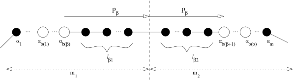
In particular $\ell_{\beta}=\ell_{{\beta}1}+\ell_{{\beta}2}$. In other words, $\beta$ is the number of $B$-elements before the time division, and $\ell_{{\beta}1},\ell_{{\beta}2}$ describe how the time division line divides the $(A\setminus B)$-elements between the $\beta$-th and $(\beta+1)$-th $B$-elements (see Figure 2; the dashed vertical line indicates the time division). We define the primed versions analogously.

Recalling (2.4) and (2.25), we have the expression:

$$\mathcal{K}_{m_{1},m_{2}} (t_{1},t_{2};{\mathfrak{p}}_{0,b}^{\mathfrak{l}_{0,b}})$$

$$= \,\mathcal{K}(t_{1};\underbrace{p_{0},\ldots,p_{0}}_{\ell_{0}+1},\ldots,\underbrace{p_{\beta},\ldots,p_{\beta}}_{\ell_{{\beta}1}+1})\mathcal{K}(t_{2};\underbrace{p_{\beta},\ldots,p_{\beta}}_{\ell_{{\beta}2}+1},\ldots,\underbrace{p_{b},\ldots,p_{b}}_{\ell_{b}+1})\,.$$

Figure 2: Time Division

In accordance with (2.40), one can check that:

$$\mathcal{K}_{m_{1},m_{2}} (t_{1},t_{2};{\mathfrak{p}}_{0,b}^{\mathfrak{l}_{0,b}})$$

$$= \int_{0}^{t_{1}*}ds_{1}d\tau_{1}\int_{0}^{t_{2}*}ds_{2}d\tau_{2}\,K_{m_{1},m_{2}}(s_{1},s_{2};{\mathfrak{p}}_{0,b}^{\mathfrak{l}_{0,b}})F_{m_{1},m_{2}}(\tau_{1},\tau_{2};{\mathfrak{p}}_{0,b}^{\mathfrak{l}_{0,b}})$$

for

$$K_{m_{1},m_{2}}(s_{1},s_{2};{\mathfrak{p}}_{0,b}^{\mathfrak{l}_{0,b}}):= K(s_{1};{\mathfrak{p}}_{0,{\beta}}^{\mathfrak{l}_{0,{\beta}1}})K(s_{2};{\mathfrak{p}}_{{\beta},b}^{\mathfrak{l}_{{\beta}2,b}})$$

$$F_{m_{1},m_{2}}(\tau_{1},\tau_{2};{\mathfrak{p}}_{0,b}^{\mathfrak{l}_{0,b}}):= F(\tau_{1};{\mathfrak{p}}_{0,{\beta}}^{\mathfrak{l}_{0,{\beta}1}})F(\tau_{2};{\mathfrak{p}}_{{\beta},b}^{\mathfrak{l}_{{\beta}2,b}})\;.$$ (3.13)

In the future, we will omit the subscripts on $\mathcal{K}_{m_{1},m_{2}}$, $K_{m_{1},m_{2}}$ and $F_{m_{1},m_{2}}$ when they are obvious from the context.

In what follows, we will adopt the following convention. We will use upper case index variables when summing over index sets of the form

$$(0,\ldots,{\beta}-1,{\beta}1,{\beta}2,{\beta}+1\ldots,b).$$

Moreover, define the upper case momenta in the following way. If ${\mathfrak{p}}_{0,b}$ is a set of momenta, the corresponding upper case momenta are defined by:

$$P_{J}:= p_{J}\qquad\mbox{for $J\neq{\beta}1,{\beta}2$}$$

$$P_{{\beta}1}= P_{{\beta}2}:=p_{{\beta}}.$$ (3.14)

Using this convention, we can write:

$$K_{m_{1},m_{2}}(s_{1},s_{2};{\mathfrak{p}}_{0,b}^{\mathfrak{l}_{0,b}})=(-i)^{b}\int_{0}^{s_{1}*}\left[d\sigma_{J}\right]_{0}^{{\beta}1}\int_{0}^{s_{2}*}\left[d\sigma_{J}\right]_{{\beta}2}^{b}\prod_{J=0}^{b}e^{-i\sigma_{J}P_{J}^{2}/2}\frac{(i\sigma_{J})^{\ell_{J}}}{\ell_{J}!}\;,$$

where the notation implies that the product is

$$\prod_{J=0}^{b}e^{-i\sigma_{J}P_{J}^{2}/2}\frac{(i\sigma_{J})^{\ell_{J}}}{\ell_{J}!}= e^{-i(\sigma_{{\beta}1}+\sigma_{{\beta}2})p_{\beta}^{2}/2}\frac{(i\sigma_{{\beta}1})^{\ell_{{\beta}1}}(i\sigma_{{\beta}2})^{\ell_{{\beta}2}}}{\ell_{{\beta}1}!\ell_{{\beta}2}!}$$

$$\times\prod_{j=0;j\neq{\beta}}^{b}e^{-i\sigma_{j}p_{j}^{2}/2}\frac{(i\sigma_{j})^{\ell_{j}}}{\ell_{j}!}\;.$$

3.1.2 Estimates on the effective potential

The next result estimates the size of the effective potential $F(\tau)$ obtained after integrating out the internal momenta (see (2.40)).

Lemma 3.4.

Let $0\leq b\leq m$ and $I\subset\{0,\ldots,b\}$ with $|I|=n\leq b+1$ and $\xi:=(\xi_{1},\ldots,\xi_{n})\in\{0,1,2\}^{n}$ be a multi-index. Let $\mathfrak{l}_{0,b}$ be as in the statement of Lemma 3.3. If $G$ is twice differentiable then there is a universal constant $M$ such that:

$$\Big{|}D^{\xi}_{{\mathfrak{p}}_{I}}\Big{(}F(\tau;{\mathfrak{p}}_{0,b}^{\mathfrak{l}_{0,b}})G({\mathfrak{p}}_{0,b})\Big{)}\Big{|}\leq\frac{(M\lambda_{0})^{m}}{\langle\tau\rangle^{3/2}}\sup_{\xi^{\prime}\in\{0,1,2\}^{n}}|D^{\xi^{\prime}}_{{\mathfrak{p}}_{I}}G({\mathfrak{p}}_{0,b})|\prod_{j=1}^{b}\frac{1}{\langle p_{j-1}-p_{j}\rangle^{26}}\;.$$

This lemma is a consequence of the dispersive estimates on the free propagator. In particular,

$$\Big{|}\int dp\,e^{-isp^{2}/2}f(p)\Big{|}\leq\|e^{is\Delta/2}\check{f}\|_{L^{\infty}}\leq Cs^{-3/2}\|\check{f}\|_{L^{1}}\leq Cs^{-3/2}\|f\|_{H^{2}}.$$

We can combine this with the trivial bound $|\int dp\,e^{-isp^{2}/2}f(p)|\leq\|f\|_{L^{1}}$ to get:

$$\Big{|}\int dp\,e^{-isp^{2}/2}f(p)\Big{|}\leq C\langle s\rangle^{-3/2}(\|f\|_{L^{1}}+\|f\|_{H^{2}}).$$

We will frequently need to apply this estimate iteratively. To do this precisely, we make some definitions. Suppose $I\subset\{0,\ldots,b\}$ of length $n$ and write $I=(i_{1},\ldots,i_{n})$. Denote by $\xi$ a multi-index of length $n$ where $\xi_{j}\in\{0,2\}$. Define the following operations on functions:

$$N^{\xi}_{d{\mathfrak{p}}_{I}}:=N^{\xi_{i_{1}}}_{dp_{i_{1}}}\circ\cdots\circ N^{\xi_{n}}_{dp_{i_{n}}} N^{0}_{dp_{j}}:=\int dp_{j}|\,\cdot\ |$$

$$N^{2}_{dp_{j}}:=\Big{(}\int dp_{j}|\,\cdot\ |^{2}\Big{)}^{1/2} \langle D_{{\mathfrak{p}}_{I}}^{\xi}\rangle:=\prod_{j=1}^{n}\langle\nabla_{p_{i_{j}}}^{\xi_{i_{j}}}\rangle$$ (3.15)

Now let $f\in\mathcal{S}(\mathbb{R}^{3(b+1)};\mathbb{C})$ and define:

$$|\!|\!|f|\!|\!|_{d{\mathfrak{p}}_{I}}:= \sum_{\xi\in\{0,2\}^{n}}N^{\xi}_{d{\mathfrak{p}}_{I}}\langle D_{{\mathfrak{p}}_{I}}^{\xi}\rangle f\;.$$ (3.16)

With this language,

$$\Big{|}\int dpe^{-isp^{2}/2}f(p)\Big{|}\leq C\langle s\rangle^{-3/2}|\!|\!|f|\!|\!|_{dp}.$$ (3.17)

We now move on to prove Lemma 3.4.

Proof.

Write ${\mathbf{k}}:={\mathbf{k}}_{m}$ and $J:=J_{m,{\mathbf{k}}_{m}}$ (recall the definition from (2.11)). From (2.40), we have:

$$D^{\xi}_{{\mathfrak{p}}_{I}}\Big{(}F (\tau;{\mathfrak{p}}_{0,b}^{\mathfrak{l}_{0,b}})G({\mathfrak{p}}_{0,b})\Big{)}=-i\sum_{k_{1},\ldots,k_{m}=0}^{\infty}\int d{\mathfrak{q}}_{J}K(\tau;{\mathfrak{q}}_{J})D^{\xi}_{{\mathfrak{p}}_{I}}\Big{(}L({\mathfrak{p}}_{0,b}^{\mathfrak{l}_{0,b}},{\mathfrak{q}}_{J})G({\mathfrak{p}}_{0,b})\Big{)}.$$

For a fixed ${\mathbf{k}}$, we have from (2.14):

$$\int d{\mathfrak{q}}_{J} K(\tau;{\mathfrak{q}}_{J})D^{\xi}_{{\mathfrak{p}}_{I}}\Big{(}L({\mathfrak{p}}_{0,b}^{\mathfrak{l}_{0,b}},{\mathfrak{q}}_{J})G({\mathfrak{p}}_{0,b})\Big{)}$$

$$= \int_{0}^{\tau*}\left[d\sigma_{jk}\right]_{jk\in J}\times(-i)^{\|{\mathbf{k}}\|}\int d{\mathfrak{q}}_{J}\prod_{jk\in J}e^{-i\sigma_{jk}q_{jk}^{2}/2}D^{\xi}_{{\mathfrak{p}}_{I}}\Big{(}L({\mathfrak{p}}_{0,b}^{\mathfrak{l}_{0,b}},{\mathfrak{q}}_{J})G({\mathfrak{p}}_{0,b})\Big{)},$$

where $\|{\mathbf{k}}\|:=\sum_{j=1}^{m}k_{j}$. Applying (3.17) iteratively, we have:

$$\Big{|}\int d{\mathfrak{q}}_{J}K(\tau; {\mathfrak{q}}_{J})D^{\xi}_{{\mathfrak{p}}_{I}}\Big{(}L({\mathfrak{p}}_{0,b}^{\mathfrak{l}_{0,b}},{\mathfrak{q}}_{J})G({\mathfrak{p}}_{0,b})\Big{)}\Big{|}$$

$$\leq C^{\|{\mathbf{k}}\|}\Big{|}\!\Big{|}\!\Big{|}D^{\xi}_{{\mathfrak{p}}_{I}}\Big{(}L({\mathfrak{p}}_{0,b}^{\mathfrak{l}_{0,b}},{\mathfrak{q}}_{J})G({\mathfrak{p}}_{0,b})\Big{)}\Big{|}\!\Big{|}\!\Big{|}_{d{\mathfrak{q}}_{J}}\int_{0}^{\tau*}\left[d\sigma_{jk}\right]_{J}\prod_{jk\in J}\frac{1}{\langle\sigma_{jk}\rangle^{3/2}}$$

$$\leq \frac{C^{\|{\mathbf{k}}\|}}{\langle\tau\rangle^{3/2}}\Big{|}\!\Big{|}\!\Big{|}D^{\xi}_{{\mathfrak{p}}_{I}}\Big{(}L({\mathfrak{p}}_{0,b}^{\mathfrak{l}_{0,b}},{\mathfrak{q}}_{J})G({\mathfrak{p}}_{0,b})\Big{)}\Big{|}\!\Big{|}\!\Big{|}_{d{\mathfrak{q}}_{J}}\;,$$

where the estimate is due to the multiple time integration defined in (2.7). Using the Leibniz rule and the triangle inequality,

$$\Big{|}\!\Big{|}\!\Big{|}D^{\xi}_{{\mathfrak{p}}_{I}}\Big{(}L({\mathfrak{p}}_{0,b}^{\mathfrak{l}_{0,b}},{\mathfrak{q}}_{J})G({\mathfrak{p}}_{0,b})\Big{)}\Big{|}\!\Big{|}\!\Big{|}_{d{\mathfrak{q}}_{J}}\leq \sum_{\xi^{\prime}\leq\xi}\binom{\xi}{\xi^{\prime}}|\!|\!|D_{{\mathfrak{p}}_{I}}^{\xi-\xi^{\prime}}L({\mathfrak{p}}_{0,b}^{\mathfrak{l}_{0,b}},{\mathfrak{q}}_{J})D^{\xi^{\prime}}_{{\mathfrak{p}}_{I}}G({\mathfrak{p}}_{0,b})|\!|\!|_{d{\mathfrak{q}}_{J}}\;,$$

where the notation $\xi^{\prime}\leq\xi$ indicates componentwise ordering and $\binom{\xi}{\xi^{\prime}}:=\binom{\xi_{1}}{\xi^{\prime}_{1}}\cdots\binom{\xi_{n}}{\xi^{\prime}_{n}}$. The form of $L({\mathfrak{p}}_{0,b}^{\mathfrak{l}_{0,b}},{\mathfrak{q}}_{J})$ in (2.13) allows us to write:

$$|\!|\!| D^{\xi-\xi^{\prime}}_{{\mathfrak{p}}_{I}}L({\mathfrak{p}}_{0,b}^{\mathfrak{l}_{0,b}},{\mathfrak{q}}_{J})|\!|\!|_{d{\mathfrak{q}}_{J}}$$

$$\leq (M\lambda_{0})^{m+\|{\mathbf{k}}\|}\int d{\mathfrak{q}}_{J}\prod_{j=1}^{m}\frac{1}{\langle r_{j-1}-q_{j1}\rangle^{30}}\frac{1}{\langle q_{j1}-q_{j2}\rangle^{30}}\cdots\frac{1}{\langle q_{jk_{j}}-r_{j}\rangle^{30}}\bigg{|}_{{\mathfrak{r}}_{0,m}={\mathfrak{p}}_{0,b}^{\mathfrak{l}_{0,b}}}$$

$$\leq (M\lambda_{0})^{m+\|{\mathbf{k}}\|}\prod_{j=1}^{b}\frac{1}{\langle p_{j-1}-p_{j}\rangle^{26}}\int d{\mathfrak{q}}_{J}\prod_{j=1}^{m}\frac{1}{\langle r_{j-1}-q_{j1}\rangle^{4}}\cdots\frac{1}{\langle q_{jk_{j}}-r_{j}\rangle^{4}}\bigg{|}_{{\mathfrak{r}}_{0,m}={\mathfrak{p}}_{0,b}^{\mathfrak{l}_{0,b}}}.$$

Summing over $k_{j}$ and using that $\lambda_{0}\ll 1$, we obtain the lemma. ∎

Define:

$$J_{1}:= (11,\ldots,1k_{1},\ldots,m_{1}1,\ldots,m_{1}k_{m_{1}})$$

$$J_{2}:= (m_{1}+1\,1,\ldots,m_{1}+1\,k_{m_{1}+1},\ldots,m1,\ldots,mk_{m}),$$ (3.18)

where the first double index in $J_{2}$ has $m_{1}+1$ as the first element and $1$ as the second, etc. This implies $J_{1}\oplus J_{2}=J_{m,{\mathbf{k}}_{m}}$. Expanding (3.13) and using (2.40) yield:

$$F_{m_{1},m_{2}}(\tau_{1},\tau_{2};{\mathfrak{p}}_{0,b}^{\mathfrak{l}_{0,b}})= -\sum_{k_{1},\ldots,k_{m}=0}^{\infty}\int d{\mathfrak{q}}_{J_{m,{\mathbf{k}}_{m}}}L({\mathfrak{p}}_{0,b}^{\mathfrak{l}_{0,b}},{\mathfrak{q}}_{J_{m,{\mathbf{k}}_{m}}})K(\tau_{1};{\mathfrak{q}}_{J_{1}})K(\tau_{2};{\mathfrak{q}}_{J_{2}}).$$

Again, the degenerate term of $k_{1}=\cdots=k_{m}=0$ of the last sum is defined as $\delta(\tau_{1})\,\delta(\tau_{2})L({\mathfrak{p}}_{0,b}^{\mathfrak{l}_{0,b}})$. A simple corollary to Lemma 3.4 is the estimate:

$$\Big{|}D^{\xi}_{{\mathfrak{p}}_{I}}\Big{(}F_{m_{1},m_{2}}( \tau_{1},\tau_{2};\,{\mathfrak{p}}_{0,b}^{\mathfrak{l}_{0,b}})G({\mathfrak{p}}_{0,b})\Big{)}\Big{|}$$

$$\leq\frac{(M\lambda_{0})^{m_{1}+m_{2}}}{\langle\tau_{1}\rangle^{3/2}\langle\tau_{2}\rangle^{3/2}}\sup_{\xi^{\prime}\in\{0,1,2\}^{n}}|D^{\xi^{\prime}}_{{\mathfrak{p}}_{I}}G({\mathfrak{p}}_{0,b})|\prod_{j=1}^{b}\frac{1}{\langle p_{j-1}-p_{j}\rangle^{26}}.$$ (3.19)

3.2 Estimate of $\varphi^{\mathrm{error,1}}(t)$

We now estimate the first error term, $\varphi^{\mathrm{error,1}}(t)$, in Lemma 3.2. We will omit the $L\to\infty$ limit from the rest of this section with the understanding, that this limit is taken in every estimate before any other limits.

Lemma 3.5.

Recall that $t=T\varepsilon^{-1}$ and $\varrho=\varepsilon\varrho_{0}$. Let $m_{0}=m_{0}(\varepsilon)\gg 1$, $n=n(\varepsilon)\gg 1$ (we will make precise choices later in (3.42) and (3.43)) and suppose $1\leq m_{1},m_{2}\leq m_{0}-1$ such that $m=m_{1}+m_{2}\geq m_{0}$. Then for $t_{1}+t_{2}=t$ with $t_{2}\geq t_{1}$, we have the bound:

$${\mathbf{E}}\|\mathcal{U}_{m_{1},m_{2}}^{\circ} (t_{1},t_{2})\psi_{0}\|^{2}$$

$$\leq C(M\lambda_{0})^{m}\langle T\rangle^{m}\Big{[}\frac{(\varrho t_{1})^{m_{1}}(\varrho t_{2})^{m_{2}}}{m_{1}!m_{2}!}+m!\varrho(\log t)^{m+\operatorname{O}(1)}(\varrho t_{1})^{m_{1}-1}(\varrho t_{2})^{m_{2}}\Big{]}.$$ (3.20)

Consequently, for $k\geq 1$:

$${\mathbf{E}}\|\varphi^{\mathrm{error,1}}_{k}(t)\|^{2}\leq C^{m_{0}}\langle T\rangle^{2m_{0}}\Big{[}\frac{1}{n}\frac{1}{m_{0}!}+(2m_{0})!\varrho(\log t)^{2m_{0}+\operatorname{O}(1)}\Big{]}\;.$$ (3.21)

Proof.

By definition (2.24), we have:

$${\mathcal{U}}^{\circ}_{m_{1},m_{2};A} (t_{1},t_{2})\psi_{0}(p_{0})$$

$$= \int d{\mathfrak{p}}_{m}\,\mathcal{K}(t_{1};{\mathfrak{p}}_{0,m_{1}})\mathcal{K}(t_{2};{\mathfrak{p}}_{m_{1},m})\chi(A;{\mathfrak{p}}_{0,m})\psi_{0}(p_{m}).$$

We apply Lemma 3.3 to get:

$${\mathbf{E}}\|\mathcal{U}_{m_{1},m_{2}}^{\circ} (t_{1},t_{2})\psi_{0}\|^{2}$$

$$\leq \sum_{b=0}^{m}\sum_{\sigma\in\operatorname{S}(b)}\sum_{\mathfrak{l},\mathfrak{l}^{\prime}}\varrho^{2m-b}\Big{|}\int dp_{0}d{\mathfrak{p}}_{b}d{\mathfrak{p}}^{\prime}_{b}\,\Delta_{\sigma}(p_{0},{\mathfrak{p}}_{b},{\mathfrak{p}}^{\prime}_{b})\psi_{0}(p_{b})\overline{\psi_{0}(p^{\prime}_{b})}$$

$$\times\mathcal{K}_{m_{1},m_{2}}(t_{1},t_{2};p_{0}^{\ell_{0}},{\mathfrak{p}}_{b}^{\mathfrak{l}_{b}})\overline{\mathcal{K}_{m_{1},m_{2}}(t_{1},t_{2};p_{0}^{\ell^{\prime}_{0}},{{\mathfrak{p}}^{\prime}_{b}}^{\mathfrak{l}^{\prime}_{b}})}\Big{|}$$

$$:= \,\mbox{(Direct)}+\mbox{(Crossing)}\;,$$ (3.22)

where

$$\mbox{(Direct)}:= \sum_{b=0}^{m}\sum_{\mathfrak{l},\mathfrak{l}^{\prime}}\varrho^{2m-b}\Big{|}\int dp_{0}d{\mathfrak{p}}_{b}\,|\psi_{0}(p_{b})|^{2}$$

$$\times\mathcal{K}(t_{1},t_{2};p_{0}^{\ell_{0}},{\mathfrak{p}}_{b}^{\mathfrak{l}_{b}})\overline{\mathcal{K}(t_{1},t_{2};p_{0}^{\ell^{\prime}_{0}},{\mathfrak{p}}_{b}^{\mathfrak{l}^{\prime}_{b}})}\Big{|}$$

$$\mbox{(Crossing)}:= \sum_{b=2}^{m}\sum_{\sigma\in\operatorname{S}(b)\setminus\operatorname{Id}}\sum_{\mathfrak{l},\mathfrak{l}^{\prime}}\varrho^{2m-b}\Big{|}\int dp_{0}d{\mathfrak{p}}_{b}d{\mathfrak{p}}^{\prime}_{b}\,\Delta_{\sigma}(p_{0},{\mathfrak{p}}_{b},{\mathfrak{p}}^{\prime}_{b})\psi_{0}(p_{b})\overline{\psi_{0}(p^{\prime}_{b})}$$

$$\times\mathcal{K}(t_{1},t_{2};p_{0}^{\ell_{0}},{\mathfrak{p}}_{b}^{\mathfrak{l}_{b}})\overline{\mathcal{K}(t_{1},t_{2};p_{0}^{\ell^{\prime}_{0}},{{\mathfrak{p}}^{\prime}_{b}}^{\mathfrak{l}^{\prime}_{b}})}\Big{|}.$$ (3.23)

The decomposition depends on whether $\sigma$ is trivial (identity) or not. When $\sigma$ is trivial, then the pairing functions (3.7) reduce to the relations $\prod_{j=1}^{b}\delta(p_{j}-{p^{\prime}}_{j})$. This decomposition will correspond to the two terms on the right hand side of estimate (3.20).

We will treat the Direct term first. Applying the Schwarz inequality and using that $\Sigma_{\mathfrak{l}^{\prime}}1=\Sigma_{\mathfrak{l}}1=\binom{m}{b}\leq 2^{m}$,

$$\mbox{(Direct)}\leq \sum_{b=0}^{m}\sum_{\mathfrak{l}}2^{m}\varrho^{2m-b}\int d{\mathfrak{p}}_{0,b}|\psi_{0}(p_{b})|^{2}|\mathcal{K}(t_{1},t_{2};{\mathfrak{p}}_{0,b}^{\mathfrak{l}_{0,b}})|^{2}.$$

Using (2.40), we can write

$$\mbox{(Direct)}\leq 2^{m}\sum_{b=0}^{m}\sum_{\mathfrak{l}}\varrho^{2m-b}\int_{0}^{t_{1}*}ds_{1}d\tau_{1}\int_{0}^{t_{1}*}ds^{\prime}_{1}d\tau^{\prime}_{1}\int_{0}^{t_{2}*}ds_{2}d\tau_{2}\int_{0}^{t_{2}*}ds^{\prime}_{2}d\tau^{\prime}_{2}$$

$$\times\int d{\mathfrak{p}}_{0,b}|\psi_{0}(p_{b})|^{2}K(s_{1},s_{2};{\mathfrak{p}}_{0,b}^{\mathfrak{l}_{0,b}})\overline{K(s^{\prime}_{1},s^{\prime}_{2};{\mathfrak{p}}_{0,b}^{\mathfrak{l}_{0,b}})}$$

$$\times F(\tau_{1},\tau_{2};{\mathfrak{p}}_{0,b}^{\mathfrak{l}_{0,b}})\overline{F(\tau^{\prime}_{1},\tau^{\prime}_{2};{\mathfrak{p}}_{0,b}^{\mathfrak{l}_{0,b}})}.$$

We now estimate the free kernel. With the index convention introduced in (3.14), we use (2.14) and (2.39) to write:

$$\int d{\mathfrak{p}}_{0,b}\, |\psi_{0}(p_{b})|^{2}K(s_{1},s_{2};{\mathfrak{p}}_{0,b}^{\mathfrak{l}_{0,b}})\overline{K(s^{\prime}_{1},s^{\prime}_{2};{\mathfrak{p}}_{0,b}^{\mathfrak{l}_{0,b}})}F(\tau_{1},\tau_{2};{\mathfrak{p}}_{0,b}^{\mathfrak{l}_{0,b}})\overline{F(\tau^{\prime}_{1},\tau^{\prime}_{2};{\mathfrak{p}}_{0,b}^{\mathfrak{l}_{0,b}})}$$

$$= \int d{\mathfrak{p}}_{0,b}\,F(\tau_{1},\tau_{2};{\mathfrak{p}}_{0,b}^{\mathfrak{l}_{0,b}})\overline{F(\tau^{\prime}_{1},\tau^{\prime}_{2};{\mathfrak{p}}_{0,b}^{\mathfrak{l}_{0,b}})}|\psi_{0}(p_{b})|^{2}$$

$$\times\int_{0}^{s_{1}*}\left[d\sigma_{J}\right]_{0}^{{\beta}1}\int_{0}^{s^{\prime}_{1}*}\left[d\sigma^{\prime}_{J}\right]_{0}^{{\beta}1}\int_{0}^{s_{2}*}\left[d\sigma_{J}\right]_{{\beta}2}^{b}\int_{0}^{s^{\prime}_{2}*}\left[d\sigma^{\prime}_{J}\right]_{\beta 2}^{b}$$

$$\times\prod_{J=0}^{b}e^{-i(\sigma_{J}-\sigma^{\prime}_{J})P_{J}^{2}/2}\frac{(\sigma_{J}\sigma^{\prime}_{J})^{\ell_{J}}}{(\ell_{J}!)^{2}}\;.$$ (3.24)

For notational convenience, assume ${\beta}\neq b$. The case $b=\beta$ is estimated in the same way. By the decay of the initial wave function in momentum space and the triangle inequality, we have:

$$\Big{|}\int d{\mathfrak{p}}_{0,b} |\psi_{0}(p_{b})|^{2}F(\tau_{1},\tau_{2};{\mathfrak{p}}_{0,b}^{\mathfrak{l}_{0,b}})\overline{F(\tau^{\prime}_{1},\tau^{\prime}_{2};{\mathfrak{p}}_{0,b}^{\mathfrak{l}_{0,b}})}\prod_{J=0}^{b}e^{-i(\sigma_{J}-\sigma^{\prime}_{J})P_{J}^{2}/2}\Big{|}$$

$$\leq \|\psi_{0}\|_{30,0}^{2}\sup_{p_{b}}\Big{|}\int d{\mathfrak{p}}_{0,b-1}F(\tau_{1},\tau_{2};{\mathfrak{p}}_{0,b}^{\mathfrak{l}_{0,b}})\overline{F(\tau^{\prime}_{1},\tau^{\prime}_{2};{\mathfrak{p}}_{0,b}^{\mathfrak{l}_{0,b}})}\langle p_{b}\rangle^{-60}$$

$$\times e^{-i[(\sigma_{\beta 1}-\sigma^{\prime}_{\beta 1})+(\sigma_{\beta 2}-\sigma^{\prime}_{\beta 2})]p_{\beta}^{2}/2}\prod_{j=0;j\neq\beta}^{b-1}e^{-i(\sigma_{j}-\sigma^{\prime}_{j})p_{j}^{2}/2}\Big{|}$$

$$\leq \|\psi_{0}\|_{30,0}^{2}C^{b}\sup_{p_{b}}|\!|\!|F(\tau_{1},\tau_{2};{\mathfrak{p}}_{0,b}^{\mathfrak{l}_{0,b}})\overline{F(\tau^{\prime}_{1},\tau^{\prime}_{2};{\mathfrak{p}}_{0,b},\ell)}\langle p_{b}\rangle^{-60}|\!|\!|_{d{\mathfrak{p}}_{0,b-1}}$$

$$\times\langle(\sigma_{\beta 1}-\sigma^{\prime}_{\beta 1})+(\sigma_{\beta 2}-\sigma^{\prime}_{\beta 2})\rangle^{-3/2}\prod_{j=0;j\neq{\beta}}^{b-1}\langle\sigma_{j}-\sigma^{\prime}_{j}\rangle^{-3/2},$$

where the last estimate used (3.17) iteratively. Applying this to (3.24), using ${\sigma^{\prime}}_{J}\leq s^{\prime}_{1}$ and $\sigma^{\prime}_{J}\leq s^{\prime}_{2}$ for $J\leq{\beta}1$ and $J>{\beta}2$, respectively, and performing the integration over $\left[d\sigma^{\prime}_{J}\right]_{0}^{{\beta}1}$ and $\left[d\sigma^{\prime}_{J}\right]_{{\beta}2}^{b}$, we have:

$$\mbox{(\ref{E:timedivfreesplit})}\leq C^{b}\sup_{p_{b}}|\!|\!|F(\tau_{1},\tau_{2};{\mathfrak{p}}_{0,b}^{\mathfrak{l}_{0,b}})\overline{F(\tau^{\prime}_{1},\tau^{\prime}_{2};{\mathfrak{p}}_{0,b}^{\mathfrak{l}_{0,b}})}\langle p_{b}\rangle^{-60}|\!|\!|_{d{\mathfrak{p}}_{0,b-1}}$$

$$\times\frac{{s^{\prime}}_{1}^{\ell_{0}+\cdots+\ell_{{\beta}1}}}{\ell_{0}!\cdots\ell_{{\beta}1}!}\frac{{s^{\prime}}_{2}^{\ell_{{\beta}2}+\cdots+\ell_{b}}}{\ell_{{\beta}2}!\cdots\ell_{b}!}\int_{0}^{s_{1}*}\left[d\sigma_{J}\right]_{0}^{\beta 1}\int_{0}^{s_{2}*}\left[d\sigma_{J}\right]_{\beta 2}^{b}\prod_{J=0}^{b}\sigma_{J}^{\ell_{J}},$$

where we have also used the trivial estimate $1/(\ell_{j})!\leq 1$. Using the identity

$$\int_{0}^{s}(s-\sigma_{j})^{m}\sigma_{j}^{\ell_{j}}d\sigma_{j}=\frac{\ell_{j}!m!}{(m+\ell_{j}+1)!}s^{m+\ell_{j}+1},$$

we have:

$$\mbox{(\ref{E:timedivfreesplit})}\leq \frac{s_{1}^{m_{1}}s_{2}^{m_{2}}t^{m-b}C^{b}}{m_{1}!m_{2}!}\sup_{p_{b}}|\!|\!|F(\tau_{1},\tau_{2};{\mathfrak{p}}_{0,b}^{\mathfrak{l}_{0,b}})\overline{F(\tau^{\prime}_{1},\tau^{\prime}_{2};{\mathfrak{p}}_{0,b}^{\mathfrak{l}_{0,b}})}\langle p_{b}\rangle^{-60}|\!|\!|_{d{\mathfrak{p}}_{0,b-1}}\,.$$

Using the definition of $|\!|\!|\cdot|\!|\!|$ and (3.19) we conclude

$$\sup_{p_{b}}|\!|\!|F(\tau_{1}, \tau_{2};{\mathfrak{p}}_{0,b}^{\mathfrak{l}_{0,b}})\overline{F(\tau^{\prime}_{1},\tau^{\prime}_{2};{\mathfrak{p}}_{0,b}^{\mathfrak{l}_{0,b}})}\langle p_{b}\rangle^{-60}|\!|\!|_{d{\mathfrak{p}}_{0,b-1}}\leq\frac{C(M\lambda_{0})^{m}}{\langle\tau_{1}\rangle^{3/2}\langle\tau_{2}\rangle^{3/2}\langle\tau^{\prime}_{1}\rangle^{3/2}\langle\tau^{\prime}_{2}\rangle^{3/2}}\;,$$

which implies

$$\mbox{(Direct)}\leq (M\lambda_{0})^{m}\sum_{b=0}^{m}\sum_{\mathfrak{l}}\varrho^{2m-b}\int_{0}^{t_{1}*}ds_{1}d\tau_{1}\int_{0}^{t_{1}*}ds^{\prime}_{1}d\tau^{\prime}_{1}\int_{0}^{t_{2}*}ds_{2}d\tau_{2}\int_{0}^{t_{2}*}ds^{\prime}_{2}d\tau^{\prime}_{2}$$

$$\times\frac{t^{m-b}}{\langle\tau_{1}\rangle^{3/2}\langle\tau^{\prime}_{1}\rangle^{3/2}\langle\tau_{2}\rangle^{3/2}\langle\tau^{\prime}_{2}\rangle^{3/2}}\frac{s_{1}^{m_{1}}}{m_{1}!}\frac{s_{2}^{m_{2}}}{m_{2}!}$$

$$\leq C(M\lambda_{0})^{m}\langle T\rangle^{m}\frac{(\varrho t_{1})^{m_{1}}(\varrho t_{2})^{m_{2}}}{m_{1}!m_{2}!}\;.$$ (3.25)

The last inequality uses $\Sigma_{b=0}^{m}\Sigma_{\mathfrak{l}}1=2^{m}$. This proves the estimate on the Direct term.

It remains to estimate the Crossing term in (3.23). We proceed in the spirit of the ”indirect” term estimates in [9] which are based on the ${\alpha}$-representation of the free kernel (Lemma 2.1). In particular, from (2.32), we have the representation

$$\mathcal{K}_{m_{1},m_{2}}(t_{1},t_{2};{\mathfrak{p}}_{0,m})= -\frac{e^{\eta_{1}t_{1}+\eta_{2}t_{2}}}{4\pi^{2}}\int\frac{d{\alpha}_{1}d{\alpha}_{2}\quad e^{-i({\alpha}_{1}t_{1}-{\alpha}_{2}t_{2})}}{({\alpha}_{1}-p_{0}^{2}/2+i\eta_{1})({\alpha}_{2}-p_{m_{1}}^{2}/2+i\eta_{2})}$$

$$\prod_{j=1}^{m_{1}}\frac{B({\alpha}_{1},p_{j-1},p_{j})}{{\alpha}_{1}-p_{j}^{2}/2+i\eta_{1}}\prod_{j=m_{1}+1}^{m}\frac{B({\alpha}_{2},p_{j-1},p_{j})}{{\alpha}_{2}-p_{j}^{2}/2+i\eta_{2}}.$$

where $\eta_{j}:=\eta(t_{j})$. To shorten our expressions, define for $k=\{1,2\}$:

$$[{\alpha}_{k},p]:={\alpha}_{k}-p_{k}^{2}/2+i\eta_{k}\,,$$ (3.26)

and its absolute value is denoted by

$$|{\alpha}_{k},p|:=|[{\alpha}_{k},p]|.$$

Analogous definitions are introduced for the primed versions with the same $\eta_{k}$ regularizations:

$$[{\alpha}_{k}^{\prime},p]:={\alpha}_{k}^{\prime}-p_{k}^{2}/2+i\eta_{k},\qquad|{\alpha}_{k}^{\prime},p|:=|[{\alpha}_{k}^{\prime},p]|\,.$$ (3.27)

Note that the regularization $\eta_{k}$ is not explicitly accounted for in the notation. However, the short notations $[\alpha,p]$, $|{\alpha},p|$ will always be used in a context when $\alpha$ equals to one of the variables $\alpha_{1},\alpha_{2},\alpha_{1}^{\prime},\alpha_{2}^{\prime}$ and the index of $\alpha$ indicates the index of the regularizing $\eta$.

Consequently, it remains to bound:

$$\sum_{b=2}^{m} \sum_{\sigma\neq\operatorname{Id}}\sum_{\mathfrak{l},\mathfrak{l}^{\prime}}\varrho^{2m-b}\Big{|}\int d{\mathfrak{p}}_{0,b}d{\mathfrak{p}}^{\prime}_{b}\,\psi_{0}(p_{b})\overline{\psi_{0}(p^{\prime}_{b})}\Delta_{\sigma}(p_{0},{\mathfrak{p}}_{b},{\mathfrak{p}}^{\prime}_{b})$$

$$\times\int d{\boldsymbol{\alpha}}d{\boldsymbol{\alpha}}^{\prime}\,e^{-i({\boldsymbol{\alpha}}-{\boldsymbol{\alpha}}^{\prime})\cdot(t_{1},t_{2})}B({\alpha}_{1},{\mathfrak{p}}_{0,{\beta}})B({\alpha}_{2},{\mathfrak{p}}_{{\beta},b})\overline{B({\alpha}^{\prime}_{1},p_{0},{\mathfrak{p}}^{\prime}_{{\beta}^{\prime}})}\overline{B({\alpha}^{\prime}_{2},{\mathfrak{p}}^{\prime}_{{\beta}^{\prime},b})}$$

$$\times\prod_{J=0}^{{\beta}1}\frac{B({\alpha}_{1},P_{J},P_{J})^{\ell_{J}}}{[{\alpha}_{1},P_{J}]^{\ell_{J}+1}}\prod_{J={\beta}2}^{b}\frac{B({\alpha}_{2},P_{J},P_{J})^{\ell_{J}}}{[{\alpha}_{2},P_{J}]^{\ell_{J}+1}}$$

$$\times\prod_{J=0}^{{\beta}^{\prime}1}\frac{\overline{B({\alpha}^{\prime}_{1},{P^{\prime}}_{J},{P^{\prime}}_{J})}^{\ell^{\prime}_{J}}}{[{\alpha}^{\prime}_{1},{P^{\prime}}_{J}]^{\ell^{\prime}_{J}+1}}\prod_{J={\beta}^{\prime}2}^{b}\frac{\overline{B({\alpha}^{\prime}_{2},{P^{\prime}}_{J},{P^{\prime}}_{J})}^{\ell^{\prime}_{J}}}{[{\alpha}^{\prime}_{2},{P^{\prime}}_{J}]^{\ell^{\prime}_{J}+1}}\Big{|}$$ (3.28)

where ${\boldsymbol{\alpha}}:=({\alpha}_{1},{\alpha}_{2})$, ${\boldsymbol{\alpha}}^{\prime}:=({\alpha}_{1}^{\prime},{\alpha}_{2}^{\prime})$ and

$$B({\alpha},{\mathfrak{p}}_{n,m}):=\prod_{j=n+1}^{m}B({\alpha},p_{j-1},p_{j}) \mbox{for $n\leq m$}.$$ (3.29)

We will now proceed as in Lemma 3.5 of [9] by exploiting the pairing relations and estimating each almost singular integral in a particular way. The technical Lemma 5.2 (to be proven later in Section 5) and the triangle inequality imply

$$\sup_{{\alpha}_{1},{\alpha}_{j}}\Big{|}B({\alpha}_{1},{\mathfrak{p}}_{0,{\beta}})B({\alpha}_{2},{\mathfrak{p}}_{{\beta},b})\Big{|}\leq\prod_{j=1}^{b}\frac{M\lambda_{0}}{\langle p_{j-1}-p_{j}\rangle^{30}}\leq\prod_{i=1}^{6}\frac{1}{\langle p_{k_{i}}\rangle^{4}}\prod_{j=1}^{b}\frac{M\lambda_{0}}{\langle p_{j-1}-p_{j}\rangle^{4}},$$ (3.30)

where $k_{i}$ are between $0$ and $b$ and can be chosen at will. The same statements hold for the primed momenta.

In general the pairing structure can be quite complicated. However, we know from Lemmas 2.4 and 2.8 of [9] that we can express the primed momenta as linear combinations of the non-primed ones, in particular:

$$\Delta_{\sigma}(p_{0},{\mathfrak{p}}_{b},{\mathfrak{p}}^{\prime}_{b})=\prod_{j=1}^{b}\delta({p^{\prime}}_{j}-l_{j}({\mathfrak{p}}_{0,b})),$$

for some linear functions $l_{j}$. Moreover, we always have the condition ${p^{\prime}}_{b}=p_{b}$. The assumption that $\sigma\neq\operatorname{Id}$ implies that there is a $0<\kappa<b$ such that $l_{{\kappa}}({\mathfrak{p}}_{0,b})$ is nontrivial. That is, there are distinct indices $\kappa_{1},\ldots,\kappa_{\iota}$ such that $p^{\prime}_{\kappa}=\pm p_{\kappa_{1}}\pm\cdots\pm p_{\kappa_{\iota}}$ where the right hand side contains at least 3 terms. Hence we can always choose $\kappa_{1},\kappa_{2}$ such that ${\kappa}_{1},{\kappa}_{2}\neq b$, and ${\kappa}_{1}\neq{\beta}$.

Suppose first that $\kappa\neq\beta^{\prime}$. Let

$${\alpha}(j):=\begin{cases}{\alpha}_{1}&\text{for $0\leq j<{\beta}$}\\ {\alpha}_{2}&\text{for ${\beta}\leq j\leq b$}\end{cases}$$

and define ${\alpha}^{\prime}(j)$ analogously, with ${\beta}^{\prime}$ in place of ${\beta}$. Define ${\alpha}({\kappa}_{1},{\kappa}_{2})^{c}$ so that

$$\{{\alpha}({\kappa}_{1}),{\alpha}({\kappa}_{2}),{\alpha}({\kappa}_{1},{\kappa}_{2})^{c}\}=\{{\alpha}_{1},{\alpha}_{2}\}.$$

In the case where $\{{\alpha}({\kappa}_{1}),{\alpha}({\kappa}_{2})\}=\{{\alpha}_{1},{\alpha}_{2}\}$ choose ${\alpha}({\kappa}_{1},{\kappa}_{2})^{c}={\alpha}_{1}$. Similarly define ${{\alpha}^{\prime}({\kappa})}^{c}$ so that $\{{\alpha}^{\prime}({\kappa}),{{\alpha}^{\prime}({\kappa})}^{c}\}=\{{\alpha}^{\prime}_{1},{\alpha}^{\prime}_{2}\}$. From (3.28), we need to bound:

$$\int d{\mathfrak{p}}_{0,b}d{\mathfrak{p}}^{\prime}_{b-1}\,\langle p_{b}\rangle^{60}|\psi_{0}(p_{b})|^{2}\prod_{j=1}^{b-1}\delta(p^{\prime}_{j}=l_{j}({\mathfrak{p}}_{0,b}))\int d{\boldsymbol{\alpha}}d{\boldsymbol{\alpha}}^{\prime}$$

$$\times\prod_{J=0}^{{\beta}1}\frac{1}{|{\alpha}_{1},P_{J}|^{\ell_{J}+1}}\prod_{J={\beta}2}^{b}\frac{1}{|{\alpha}_{2},P_{J}|^{\ell_{J}+1}}\prod_{J=0}^{{\beta}^{\prime}1}\frac{1}{|{\alpha}^{\prime}_{1},P^{\prime}_{J}|^{\ell^{\prime}_{J}+1}}\prod_{J={\beta}^{\prime}2}^{b}\frac{1}{|{\alpha}^{\prime}_{2},P^{\prime}_{J}|^{\ell^{\prime}_{J}+1}}$$

$$\times\prod_{i=1}^{6}\frac{1}{\langle p_{k_{i}}\rangle^{4}\langle p^{\prime}_{k^{\prime}_{i}}\rangle^{4}}\prod_{j=1}^{b}\frac{M\lambda_{0}}{\langle p_{j-1}-p_{j}\rangle^{4}\langle{p^{\prime}}_{j-1}-{p^{\prime}}_{j}\rangle^{4}}.$$ (3.31)

First choose $k^{\prime}_{1}={\kappa}$, $k_{1}={\kappa}_{1}$ and $k_{2}={\kappa}_{2}$. We begin by using (3.8) and making the bound:

$$\sup_{\stackrel{{\scriptstyle{\alpha}^{\prime}_{1},{\alpha}_{2}}}{{p_{0},p_{b},{\mathfrak{p}}^{\prime}_{b-1}}}} \Big{[}\frac{\langle{{\alpha}^{\prime}({\kappa})}^{c}\rangle}{\langle p^{\prime}_{k^{\prime}_{2}}\rangle^{4}}\frac{1}{|{\alpha}^{\prime}_{1},{p^{\prime}}_{{\beta}^{\prime}}|^{\ell^{\prime}_{{\beta}^{\prime}1}}|{\alpha}^{\prime}_{2},{p^{\prime}}_{{\beta}^{\prime}}|^{\ell^{\prime}_{{\beta}^{\prime}2}}}\frac{1}{|{\alpha}^{\prime}_{2},p_{b}|^{\ell^{\prime}_{b}}}\frac{1}{|{\alpha}^{\prime}({\kappa}),{p^{\prime}}_{{\kappa}}|^{\ell^{\prime}_{\kappa}}}$$

$$\times\frac{1}{|{\alpha}^{\prime}_{2},{p^{\prime}}_{{\beta}^{\prime}}|}\prod_{\stackrel{{\scriptstyle 0\leq j\leq b-1}}{{j\neq{\kappa},{\beta}^{\prime}}}}\frac{1}{|{\alpha}^{\prime}(j),{p^{\prime}}_{j}|^{\ell^{\prime}_{j}+1}}\Big{]}\leq Ct_{1}^{m_{1}-1}t_{2}^{m_{2}}\,.$$

(In case of $\kappa=\beta^{\prime}$ the first term on the second line is omitted.) Indeed, this estimate follows as we can pick $k^{\prime}_{2}$ such that $|{{\alpha}^{\prime}({\kappa})}^{c},{p^{\prime}}_{k^{\prime}_{2}}|^{-1}$ is a factor in the above product. We then apply (2.36) to obtain

$$\sup_{{{\alpha}^{\prime}({\kappa})}^{c},{p^{\prime}}_{k^{\prime}_{2}}}\frac{\langle{{\alpha}^{\prime}({\kappa})}^{c}\rangle}{\langle{p^{\prime}}_{k^{\prime}_{2}}\rangle^{4}|{{\alpha}^{\prime}({\kappa})}^{c},{p^{\prime}}_{k^{\prime}_{2}}|}\leq\begin{cases}Ct_{1}&\text{if ${\kappa}\geq{\beta}^{\prime}$}\\ Ct_{2}&\text{if ${\kappa}<{\beta}^{\prime}$}\end{cases}$$

while using (2.38) on the remaining factors and applying $t_{1}\leq t_{2}$. After estimating the initial wave function, $\|\psi_{0}\|^{2}_{30,0}\leq C$, we obtain

$$\mbox{(\ref{E:crossingstart})}\leq Ct_{1}^{m_{1}-1}t_{2}^{m_{2}}\sup_{p_{b}}\int d{\mathfrak{p}}_{0,b-1}d{\mathfrak{p}}^{\prime}_{b-1}\prod_{j=1;j\neq{\kappa}}^{b-1}\delta({p^{\prime}}_{j}=l_{j}({\mathfrak{p}}_{0,b}))$$

$$\times\int\frac{d{\alpha}_{1}}{\langle{\alpha}_{1}\rangle|{\alpha}_{1},p_{\beta}|}\int\frac{d{\alpha}_{2}}{\langle{\alpha}_{2}\rangle|{\alpha}_{2},p_{b}|}\int\frac{d{\alpha}^{\prime}_{1}}{\langle{\alpha}^{\prime}_{1}\rangle|{\alpha}^{\prime}_{1},{p^{\prime}}_{{\beta}^{\prime}}|}\int\frac{d{\alpha}^{\prime}_{2}}{\langle{\alpha}^{\prime}_{2}\rangle|{\alpha}^{\prime}_{2},p_{b}|}$$

$$\times\frac{\delta({p^{\prime}}_{\kappa}=\pm p_{{\kappa}_{1}}\pm p_{{\kappa}_{2}}\pm\cdots)}{|{\alpha}^{\prime}({\kappa}),{p^{\prime}}_{\kappa}|\,|{\alpha}({\kappa}_{1}),p_{{\kappa}_{1}}|\,|{\alpha}({\kappa}_{2}),p_{{\kappa}_{2}}|}\frac{\langle{\alpha}({\kappa}_{1})\rangle\langle{\alpha}({\kappa}_{2})\rangle\langle{\alpha}^{\prime}({\kappa})\rangle}{\langle{p^{\prime}}_{\kappa}\rangle^{4}\langle p_{{\kappa}_{1}}\rangle^{4}\langle p_{{\kappa}_{2}}\rangle^{4}}\,\frac{\langle{\alpha}({\kappa}_{1},{\kappa}_{2})^{c}\rangle}{\langle p_{k_{3}}\rangle^{4}}$$

$$\times\underbrace{\frac{1}{|{\alpha}_{1},p_{\beta}|^{\ell_{{\beta}1}}|{\alpha}_{2},p_{\beta}|^{\ell_{{\beta}2}}}\prod_{j=0;j\neq{\beta}}^{b}\frac{1}{|{\alpha}(j),p_{j}|^{\ell_{j}}}}_{=:(i)}$$

$$\times\underbrace{\prod_{\stackrel{{\scriptstyle j=0}}{{j\neq{\kappa}_{1},{\kappa}_{2}}}}^{b-1}\frac{1}{|{\alpha}(j),p_{j}|}\prod_{i=4}^{6}\frac{1}{\langle p_{k_{i}}\rangle^{4}}\prod_{j=1}^{b}\frac{M\lambda_{0}}{\langle p_{j-1}-p_{j}\rangle^{4}}}_{=:(ii)}.$$

By our assumptions that $m_{1},m_{2}\geq 1$ and $m_{1}+m_{2}\geq m_{0}$, we can choose $k_{3}$ so that the factor $|{\alpha}({\kappa}_{1},{\kappa}_{2})^{c},p_{k_{3}}|^{-1}$ appears in either $(i)$, $(ii)$ or both. We now use (2.38) to estimate the factors in $(i)$. If $|{\alpha}({\kappa}_{1},{\kappa}_{2})^{c},p_{k_{3}}|^{-1}$ appears in (i) (for some choice of $k_{3}$), we estimate this term by (2.36):

$$\sup_{{\alpha}({\kappa}_{1},{\kappa}_{2})^{c},p_{k_{3}}}\frac{\langle{\alpha}({\kappa}_{1},{\kappa}_{2})^{c}\rangle}{\langle p_{k_{3}}\rangle^{4}|{\alpha}({\kappa}_{1},{\kappa}_{2})^{c},p_{k_{3}}|}\leq\begin{cases}Ct_{1}&\text{if ${\kappa}_{1}\geq{\beta}$}\\ Ct_{2}&\text{if ${\kappa}_{1}<{\beta}$}\;.\end{cases}$$

Either way, we apply (3.8) to produce the bound $(i)\leq t^{m-b}$. Next, we integrate ${p^{\prime}}_{j}$ for $1\leq j\leq b-1$ except for ${\kappa}$, thus removing their corresponding delta functions. We then bound:

$$\mbox{(\ref{E:crossingstart})}\leq Ct_{1}^{m_{1}-1}t_{2}^{m_{2}}t^{m-b}\sup_{p_{b}}\Big{[}\int\frac{d{\alpha}_{2}}{\langle{\alpha}_{2}\rangle\,|{\alpha}_{2},p_{b}|}\frac{d{\alpha}^{\prime}_{2}}{\langle{\alpha}^{\prime}_{2}\rangle\,|{\alpha}^{\prime}_{2},p_{b}|}\int\frac{d{\alpha}_{1}}{\langle{\alpha}_{1}\rangle}\int\frac{d{\alpha}^{\prime}_{1}}{\langle{\alpha}^{\prime}_{1}\rangle}\int d{\mathfrak{p}}_{0,b-1}$$

$$\times\frac{\delta({p^{\prime}}_{\kappa}=p_{{\kappa}_{1}}\pm p_{{\kappa}_{2}}\pm\cdots)}{|{\alpha}^{\prime}({\kappa}),{p^{\prime}}_{\kappa}|\,|{\alpha}({\kappa}_{1}),p_{{\kappa}_{1}}|\,|{\alpha}({\kappa}_{2}),p_{{\kappa}_{2}}|}\frac{\langle{\alpha}({\kappa}_{1})\rangle\langle{\alpha}^{\prime}({\kappa})\rangle\langle{\alpha}({\kappa}_{2})\rangle}{\langle{p^{\prime}}_{\kappa}\rangle^{4}\langle p_{{\kappa}_{1}}\rangle^{4}\langle p_{{\kappa}_{2}}\rangle^{4}}$$

$$\times\frac{1}{|{\alpha}^{\prime}_{1},l_{{\beta}^{\prime}}({\mathfrak{p}}_{0,b})|}\frac{1}{|{\alpha}_{1},p_{{\beta}}|}\times\,(ii^{\prime})\Big{]}$$ (3.32)

where $(ii^{\prime})$ is $(ii)$ multiplied by $\langle{\alpha}({\kappa}_{1},{\kappa}_{2})^{c}\rangle/\langle p_{k_{3}}\rangle^{4}$ if that factor was not used in the estimate of $(i)$.

In this case we choose $k_{3}$ so that $|{\alpha}({\kappa}_{1},{\kappa}_{2})^{c},p_{k_{3}}|$ appears in (ii). We next integrate ${p^{\prime}}_{{\kappa}}$ which identifies ${p^{\prime}}_{{\kappa}}=p_{{\kappa}_{1}}\pm p_{{\kappa}_{2}}\pm\cdots$. If $g=g(|p_{{\kappa}_{1}}|)$ is a non-negative function of $|p_{{\kappa}_{1}}|$, we have the estimate with $r=|p|$:

$$\int\frac{dp_{{\kappa}_{1}}}{\langle p_{{\kappa}_{1}}\rangle^{4}} \frac{\langle{\alpha}^{\prime}({\kappa})\rangle g(|p_{{\kappa}_{1}}|)}{|{\alpha}^{\prime}({\kappa}),p_{{\kappa}_{1}}\pm p_{{\kappa}_{2}}\pm\cdots|\;|\alpha(\kappa_{1}),p_{\kappa_{1}}|\,\langle p_{{\kappa}_{1}}\pm p_{{\kappa}_{2}}\pm\cdots\rangle^{4}}$$

$$\leq\int_{0}^{\infty}\frac{dr\,r}{\langle r\rangle^{4}}\frac{1}{|{\alpha}({\kappa}_{1}),r|}\frac{g(r)}{|p_{{\kappa}_{2}}\pm\cdots|},$$ (3.33)

where we have abused the notation and wrote $|{\alpha},|p||=|{\alpha},p|$. Indeed this follows from parametrizing the angular component of $p_{{\kappa}_{1}}$ relative to that of $\pm p_{{\kappa}_{2}}\pm\cdots$ and performing the angular integration exactly as in the proof of Proposition 2.3.

To apply (3.33), we choose $k_{4}={\kappa}_{1}-1$ in (3.30), and we can make the last line in (3.32) independent of the angular variable of $p_{{\kappa}_{1}}$ by estimating $\langle p_{{\kappa}_{1}-1}-p_{{\kappa}_{1}}\rangle^{-1}\leq 1$. The decay in the variable $p_{k_{4}}=p_{\kappa_{1}-1}$ is lost, but it is restored by the additional factor $\langle p_{k_{4}}\rangle^{-4}$. Our choice of $k_{4}$ will assure that we have enough decay factors to perform the necessary integrations. We obtain

$$\mbox{(\ref{E:crossingstart})}\leq Ct_{1}^{m_{1}-1}t_{2}^{m_{2}}t^{m-b}\log t\times\sup_{p_{b}}\Big{[}\int\frac{d{\alpha}_{2}}{\langle{\alpha}_{2}\rangle|{\alpha}_{2},p_{b}|}\frac{d{\alpha}^{\prime}_{2}}{\langle{\alpha}^{\prime}_{2}\rangle|{\alpha}^{\prime}_{2},p_{b}|}\int\frac{d{\alpha}_{1}}{\langle{\alpha}_{1}\rangle}\int\frac{d{\alpha}^{\prime}_{1}}{\langle{\alpha}^{\prime}_{1}\rangle}$$

$$\int d{\mathfrak{p}}_{0,{\kappa}_{1}-1}d{\mathfrak{p}}_{{\kappa}_{1}+1,b-1}\frac{\langle{\alpha}({\kappa}_{2})\rangle}{|{\alpha}({\kappa}_{2}),p_{{\kappa}_{2}}|}\int\frac{d|p_{{\kappa}_{1}}|\,\,|p_{{\kappa}_{1}}|}{\langle|p_{{\kappa}_{1}}|\rangle^{4}}\frac{\langle{\alpha}({\kappa}_{1})\rangle}{|{\alpha}({\kappa}_{1}),|p_{{\kappa}_{1}}||}\frac{1}{|p_{{\kappa}_{2}}\pm\cdots|}$$

$$\frac{1}{|{\alpha}^{\prime}_{1},l_{{\beta}^{\prime}}|}\frac{1}{|{\alpha}_{1},p_{{\beta}}|}\times\,(ii^{\prime\prime})\Big{]},$$

where $(ii^{\prime\prime})$ is the same as $(ii^{\prime})$ with $\langle p_{{\kappa}_{1}-1}-p_{{\kappa}_{1}}\rangle^{-4}$ majorized by $1$ and $k_{4}={\kappa}_{1}-1$.

We then apply (2.34) twice to make the bound:

$$\sup_{{\mathfrak{p}}_{0,b}}\Big{(}\int\frac{d{\alpha}^{\prime}_{1}}{\langle{\alpha}^{\prime}_{1}\rangle|{\alpha}^{\prime}_{1},l_{{\beta}^{\prime}}|}\int\frac{d{\alpha}^{\prime}_{2}}{\langle{\alpha}^{\prime}_{2}\rangle|{\alpha}^{\prime}_{2},p_{b}|}\Big{)}\leq C(\log t)^{2}.$$

We can now integrate $|p_{{\kappa}_{1}}|$ and then choose coordinates for $p_{{\kappa}_{2}}$ so that its angular component is parametrized relative to that of $p_{{\kappa}_{3}}\pm\cdots\pm p_{{\kappa}_{\iota}}$. Choosing $k_{5}={\kappa}_{2}-1$ and using $\langle p_{{\kappa}_{2}-1}-p_{{\kappa}_{2}}\rangle^{-4}\leq 1$ makes the remaining terms independent of this angle. We then integrate the angle, as done before, allowing us to integrate the remaining $p_{j}$ except for $p_{\beta}$. The integration is handled using (2.37) in all instances except possibly one: in the case where $(ii^{\prime})$ contains $\langle{\alpha}({\kappa}_{1},{\kappa}_{2})^{c}\rangle/\langle p_{k_{3}}\rangle^{4}$, we use (2.35) to handle this term. Since $|{\alpha}_{1},p_{\beta}|\neq|{\alpha}({\kappa}_{2}),|p_{{\kappa}_{2}}|\;|$ we can use (2.34) to bound

$$\int\frac{d{\alpha}_{1}}{\langle{\alpha}_{1}\rangle|{\alpha}_{1},p_{\beta}|}\leq C\log t,$$

while integrating $|{\alpha}_{2},p_{{\beta}}|^{-1}$ and completing the integration of $|p_{{\kappa}_{2}}|$ produces $\log$ factors. The order in which this is done will depend on whether or not ${\beta}={\kappa}_{2}$. Finally we use (2.34) to estimate

$$\sup_{p_{b}}\int\frac{d{\alpha}_{2}}{\langle{\alpha}_{2}\rangle|{\alpha}_{2},p_{b}|}\leq C\log t.$$

Collecting these estimates completes the proof in the case where ${\kappa}\neq{\beta}^{\prime}$. The case ${\kappa}={\beta}^{\prime}$ is easier to handle and can done as above. Consequently,

$$\mbox{(\ref{E:crossingstart})}\leq C(M\lambda_{0})^{2b}t^{m-b}t_{1}^{m_{1}-1}t_{2}^{m_{2}}(\log t)^{m+\operatorname{O}(1)},$$

which applied in (3.28), proves the first statement of Lemma 3.5. The second statement can be easily deduced from the first. ∎

3.3 Estimate of $\varphi^{\mathrm{error,2}}_{k}$

We next prove the amputated version of the preceding lemma which will be used, by setting $m_{1}=m_{0}$, to estimate $\varphi^{\mathrm{error,2}}_{k}$ in (3.3).

Lemma 3.6.

Suppose, $m_{1}>2$, $0\leq m_{2}<m_{0}$ and define $m=m_{1}+m_{2}$. Let $t_{1}\leq t_{2}$ and $t_{1}+t_{2}=t=T\varepsilon^{-1}$ for $k\geq 1$. We then have the bound:

$$\sup_{0\leq s\leq t_{1}} {\mathbf{E}}\|{\widetilde{\mathcal{U}}}_{m_{1},m_{2}}(s,t_{2})\psi_{0}\|^{2}$$

$$\leq C(M\lambda_{0})^{m}\langle T\rangle^{m}\Big{[}\frac{\varrho(\varrho t_{1})^{m_{1}-1}(\varrho t_{2})^{m_{2}}}{(m_{1}-1)!m_{2}!}+m!\varrho^{2}(\varrho t_{1})^{m_{1}-2}(\varrho t_{2})^{m_{2}}(\log t)^{m+\operatorname{O}(1)}\Big{]}$$

It then follows that:

$${\mathbf{E}}\|\varphi_{k}^{\mathrm{error,2}}(t)\|^{2}\leq C^{m_{0}}\langle T\rangle^{2m_{0}}\Big{[}\frac{t}{n^{m_{0}}m_{0}!}+\frac{(2m_{0})!(\log t)^{2m_{0}+\operatorname{O}(1)}}{n^{m_{0}}}\Big{]}$$

Proof.

The proof of the first statement is almost identical to the proof of Lemma 3.5 only that we replace

$$\mathcal{K}_{m_{1},m_{2}}(t_{1},t_{2};{\mathfrak{p}}_{0,m})\qquad\mbox{with}\qquad\hat{V}_{0}(p_{0}-p_{1})\mathcal{K}_{m_{1}-1,m_{2}}(t_{1},t_{2};{\mathfrak{p}}_{1,m}).$$

The missing $p_{0}$ in the latter free kernel effectively eliminates a power of $t_{1}$ from the estimate of Lemma 3.5 and also reduces the effect of $m_{1}$ by one in the estimate.

As a technical note, the crossing estimates which are done with the aid of the ${\alpha}$-representation (Lemma 2.1) require the kernel to have at least two momentum variables. Usually this amounts to requiring $m_{j}>0$ for $j=1,2$. In the previous lemma, this was avoided by assumption. However, in this case, it is possible that $m_{2}=0$. Accordingly, we do not expand the kernel $\mathcal{K}_{m_{2}}(t_{2})$ with Lemma 2.1 but use the trivial estimate $|\mathcal{K}_{0}(t_{2};r_{b})|\leq 1$ thus reducing our estimates to those without time division. Otherwise, the proof of the first statement follows in the exact same way as the previous lemma.

To prove the second statement, we recall from the defintion (2.28) that

$${\mathcal{U}}_{m_{1},m_{2}}(t_{1},t_{2})\psi_{0}=\int_{0}^{t_{1}}ds\;e^{-i(t_{1}-s)H}{\widetilde{\mathcal{U}}}_{m_{1},m_{2}}(s,t_{2})\psi_{0}\;.$$

A simple consequence of the unitarity of $e^{-i(t_{1}-s)H}$ implies

$${\mathbf{E}}\|{\mathcal{U}}_{m_{1},m_{2}}(t_{1},t_{2})\psi_{0}\|^{2}\leq t_{1}^{2}\sup_{0\leq s\leq t_{1}}{\mathbf{E}}\|{\widetilde{\mathcal{U}}}_{m_{1},m_{2}}(s,t_{2})\psi_{0}\|^{2}.$$ (3.34)

The first part of the lemma with $t_{1}=t/n$, $t_{2}=(k-1)t/n$ and $m_{1}=m_{0}$ yields:

$${\mathbf{E}}\|\varphi_{k}^{\mathrm{error,2}}(t)\|^{2}\leq m_{0}^{2}t_{1}^{2}\sum_{m_{2}=0}^{m_{0}-1}{\mathbf{E}}\|{\widetilde{\mathcal{U}}}_{m_{0},m_{2}}(t_{1},t_{2})\psi_{0}\|^{2}$$

$$\leq C^{m_{0}}\langle T\rangle^{2m_{0}}\Big{[}\frac{t}{n^{m_{0}}m_{0}!}+\frac{(2m_{0})!(\log t)^{2m_{0}+5}}{n^{m_{0}}}\Big{]}\;.$$

∎

3.4 Estimate of $\varphi^{\mathrm{error,3}}_{k}$

We now move on to estimate the third error term in (3.3). As a rule of thumb, a genuine recollision will allow us to argue as in the estimates of the crossing term in Lemma 3.5 to eliminate a power of $t_{1}$. However we will obtain a factor of $t_{1}^{2}$ when we apply crude estimates such as (3.34). Since the amputation effectively eliminates one power of $t_{1}$ (as in Lemma 3.6), this term will be $\operatorname{O}(n^{-2})$ when $m_{1}$ is small. After summing on $k$ in (2.23), our error term will be $\operatorname{O}(1)$ at best, which is not sufficient. Consequently, we are forced to continue the Duhamel expansion.

The idea is that we will keep expanding until we either obtain another genuine recollision or we get a new collision center. The latter will produce another factor of $n^{-1}$ so that after summation on $k$ in (2.23) our term will be $\operatorname{O}(n^{-1})$ and by choosing $n$ to be sufficiently large, this term will vanish in the limit. The case of a second recollision should be smaller by a power of time, which guarantees that this term vanishes in the limit. Intuitively, in order to have recollisions, obstacles need to be within a close vicinity of one another. Hence terms with these collision histories should be small since the probability of such configurations is higher order. If the obstacles were not within a close proximity with one another, then the wave function would need to travel very far to recollide and again, classically, we should be able to argue that the respective term is higher order.

However, there is a technical difficulty which presents itself here. Viewing things classically, it is possible that two obstacles are $\operatorname{O}(1)$ distance apart. When this happens, our wave can collide with these obstacles one after another in succession (of two or more times) and give the appearance of undergoing only one recollision. Though the probability that the obstacles have this configuration is $\varrho=\operatorname{O}(\varepsilon)$, this factor is not sufficient to compensate the loss in our unitary estimate. Consequently, we need effectively sum up the two-obstacle Born series to account for this. Not all pairs of recollisions need to be treated in this manner. If the original collision sequence is given by $({\alpha}_{1},\ldots,{\alpha}_{m})$ and we obtain a new collision center which is a recollision at ${\alpha}_{{\kappa}_{1}}$ followed by another new collision center which is a recollision at ${\alpha}_{{\kappa}_{2}}$, we will immediately be able to argue that the terms corresponding to the case where ${\kappa}_{2}>{\kappa}_{1}$ are small on the basis that this collision pattern is higher order. Indeed, in order to have a genuine recollision and not an internal collision, we need ${\kappa}_{1}\geq 2$. This implies that there is at least one more obstacle in the vicinity of ${\alpha}_{{\kappa}_{1}}$ and ${\alpha}_{{\kappa}_{2}}$. The probability of this configuration occurring is higher order. Hence we will only sum the two-obstacle Born series in the case where ${\kappa}_{2}<{\kappa}_{1}$ (they can never be equal since we already summed over internal collisions).

Before we precisely describe the final stopping rule for our Duhamel expansion, we need to define propagators associated to more complicated collision patterns. Given $A$ of size $m$, let $m_{1}$ and $m_{2}$ be non-negative integers with $m_{1}+m_{2}=m$. For $n_{1}\geq 2$ define:

$$\mathcal{A}(n_{1}):=\underbrace{(\ldots,{\alpha}_{{\kappa}_{1}},{\alpha}_{{\kappa}_{2}},{\alpha}_{{\kappa}_{1}})}_{n_{1}}$$

This will be the sequence of centers associated to the pair collision mentioned above. The propagator associated with the pair recollision is defined as

$${\mathcal{U}}^{\circ;{\kappa}_{1},{\kappa}_{2}}_{[n_{1}],m_{1},m_{2};A}(t_{1},t_{2})\psi_{0}(p_{0})$$

$$\qquad:=\int d{\mathfrak{u}}_{0,n_{1}-2}d{\mathfrak{r}}_{0,m}\mathcal{K}_{n_{1}+m_{1},m_{2}}(t_{1},t_{2};p_{0},{\mathfrak{u}}_{0,n_{1}-2},{\mathfrak{r}}_{0,m})$$

$$\qquad\qquad\times\chi(\mathcal{A}(n_{1})\oplus A;p_{0},{\mathfrak{u}}_{0,n_{1}-2},{\mathfrak{r}}_{0,m})\psi_{0}(r_{m})\,,$$ (3.35)

The number $n_{1}$ in brackets indicates the number of pair recollisions. For the free propagator kernel we applied he definition (2.25) in the following form

$$\mathcal{K}_{n_{1}+m_{1},m_{2}}(t_{1},t_{2};p_{0},{\mathfrak{u}}_{0,n_{1}-2},{\mathfrak{r}}_{0,m})=\mathcal{K}_{n_{1}+m_{1}}(t_{1};p_{0},{\mathfrak{u}}_{0,n_{1}-2},{\mathfrak{r}}_{0,m_{1}})\mathcal{K}_{m_{2}}(t_{2};{\mathfrak{r}}_{m_{1},m})\;$$

(see Figure 3 for the order of momentum variables).

Figure 3: Resummation of two obstacles

Summing over $1\leq{\kappa}_{2}<{\kappa}_{1}\leq m$ and $A$ gives:

$${\mathcal{U}}^{\circ}_{[n_{1}],m_{1},m_{2}}(t_{1},t_{2}):=\sum_{\stackrel{{\scriptstyle{\kappa}_{1},{\kappa}_{2}}}{{1\leq{\kappa}_{2}<{\kappa}_{1}\leq m}}}\sum_{A:|A|=m}{\mathcal{U}}^{\circ;{\kappa}_{1},{\kappa}_{2}}_{[n_{1}],m_{1},m_{2};A}(t_{1},t_{2})\;.$$

The propagators for $n_{1}=1$ are defined as:

$${\mathcal{U}}^{\circ;{\kappa}}_{[1],m_{1},m_{2};A}(t_{1},t_{2})\psi_{0}:= \int\!\!d{\mathfrak{r}}_{0,m}\,\mathcal{K}_{m_{1}+1,m_{2}}(t_{1},t_{2};p_{0},{\mathfrak{r}}_{0,m})\chi({\alpha}_{{\kappa}}\oplus A;p_{0},{\mathfrak{r}}_{0,m})\psi_{0}(r_{m})\,,$$

$${\mathcal{U}}^{\circ}_{[1],m_{1},m_{2}}(t_{1},t_{2}):= \sum_{{\kappa}=2}^{m}\sum_{A:|A|=m}{\mathcal{U}}^{\circ;{\kappa}}_{[1],m_{1},m_{2};A}(t_{1},t_{2}).$$

Note that these are the fully expanded versions of the truncated one recollision terms (3.1) and (3.2).

We will also need to define the amputated version of the two recollision propagator:

$${\widetilde{\mathcal{U}}}^{{\kappa}_{1},{\kappa}_{2}}_{[n_{1}],m_{1},m_{2};A}(t_{1},t_{2})\psi_{0}$$

$$\qquad:=\int d{\mathfrak{u}}_{0,n_{1}-2}d{\mathfrak{r}}_{0,m}\hat{V}_{0}(p_{0}-u_{0})\mathcal{K}_{n_{1}+m_{1}-1,m_{2}}(t_{1},t_{2};{\mathfrak{u}}_{0,n_{1}-2},{\mathfrak{r}}_{0,m})$$

$$\qquad\qquad\times\chi(\mathcal{A}(n_{1})\oplus A;p_{0},{\mathfrak{u}}_{0,n_{1}-2},{\mathfrak{r}}_{0,m})\psi_{0}(r_{m})$$ (3.36)

and

$${\widetilde{\mathcal{U}}}^{{\kappa}_{1},{\kappa}_{2}}_{[n_{1}],m_{1},m_{2}}(t_{1},t_{2})=\sum_{A:|A|=m}{\widetilde{\mathcal{U}}}^{{\kappa}_{1},{\kappa}_{2}}_{[n_{1}],m_{1},m_{2};A}(t_{1},t_{2})\;.$$

The next propagators are associated with the pair recollision pattern followed by a new collision with $\alpha_{0}$. For $n_{1}\geq 2$ we define:

$${\widetilde{\mathcal{U}}}^{{\kappa}_{1},{\kappa}_{2}}_{[n_{1}],m_{1},m_{2};{\alpha}_{0},A}(t_{1},t_{2})\psi_{0}(p_{0})$$

$$\qquad\quad:=\int dp_{1}d{\mathfrak{u}}_{0,n_{1}-2}d{\mathfrak{r}}_{0,m}\hat{V}_{0}(p_{0}-p_{1})\mathcal{K}_{n_{1}+m_{1},m_{2}}(t_{1},t_{2};p_{1},{\mathfrak{u}}_{n_{1}-2},{\mathfrak{r}}_{0,m})$$

$$\qquad\qquad\times\chi({\alpha}_{0}\oplus\mathcal{A}(n_{1})\oplus A;{\mathfrak{p}}_{0,1},{\mathfrak{r}}_{0,m})\psi_{0}(r_{m})$$ (3.37)

and the summed up version:

$${\widetilde{\mathcal{U}}}_{1,[n_{1}],m_{1},m_{2}}(t_{1},t_{2}):=\sum_{\stackrel{{\scriptstyle{\kappa}_{1},{\kappa}_{2}}}{{1\leq{\kappa}_{2}<{\kappa}_{1}\leq m}}}\sum_{\hat{A}:|\hat{A}|=m+1}{\widetilde{\mathcal{U}}}^{{\kappa}_{1},{\kappa}_{2}}_{[n_{1}],m_{1},m_{2};{\alpha}_{0},A}(t_{1},t_{2})$$

where the sum is over sets $\hat{A}:={\alpha}_{0}\oplus A$ with non-repeating indices. Note that the order of subscripts, $1,[n_{1}],m_{1},m_{2}$ indicate the chronological order of the collision types, the bracket indicates the number of pair recollisions.

For the special case $n_{1}=1$ the propagators are defined as:

$${\widetilde{\mathcal{U}}}^{{\kappa}}_{[1],m_{1},m_{2};{\alpha}_{0},A}(t_{1},t_{2})\psi_{0}:= \int d{\mathfrak{p}}_{0,1}d{\mathfrak{r}}_{0,m}\mathcal{K}_{m_{1}+1,m_{2}}(t_{1},t_{2};p_{1},{\mathfrak{r}}_{0,m})$$

$$\times\chi({\alpha}_{0}\oplus{\alpha}_{{\kappa}}\oplus A;{\mathfrak{p}}_{0,1},{\mathfrak{r}}_{0,m})\psi_{0}(r_{m})\,.$$

and

$${\widetilde{\mathcal{U}}}_{1,[1],m_{1},m_{2}}(t_{1},t_{2}):=\sum_{{\kappa}=2}^{m}\sum_{\hat{A}:|\hat{A}|=m+1}{\widetilde{\mathcal{U}}}^{{\kappa}}_{[1],m_{1},m_{2};{\alpha}_{0},A}(t_{1},t_{2}).$$

Finally we have the propagators corresponding to the pair recollisions followed by a genuine recollision with $\alpha_{{\kappa}_{3}}$:

$${\widetilde{\mathcal{U}}}^{{\kappa}_{1},{\kappa}_{2},{\kappa}_{3}}_{*,[n_{1}],m_{1},m_{2};A}(t_{1},t_{2})\psi_{0}(p_{0})$$

$$\qquad\quad:=\int dp_{1}d{\mathfrak{u}}_{0,n_{1}-2}d{\mathfrak{r}}_{0,m}\hat{V}_{0}(p_{0}-p_{1})\mathcal{K}_{n_{1}+m_{1},m_{2}}(t_{1},t_{2};p_{1},{\mathfrak{u}}_{n_{1}-2},{\mathfrak{r}}_{0,m})$$

$$\qquad\qquad\times\chi({\alpha}_{{\kappa}_{3}}\oplus\mathcal{A}(n_{1})\oplus A;{\mathfrak{p}}_{0,1},{\mathfrak{u}}_{0,n_{1}-2},{\mathfrak{r}}_{0,m})\psi_{0}(r_{m}),$$ (3.38)

and

$${\widetilde{\mathcal{U}}}_{*,[n_{1}],m_{1},m_{2}}(t_{1},t_{2}):=\sum_{{\kappa}_{1}=2}^{m}\sum_{{\kappa}_{2}=1}^{{\kappa}_{1}-1}\sum_{\stackrel{{\scriptstyle{\kappa}_{3}=1}}{{{\kappa}_{3}\neq{\kappa}_{1},{\kappa}_{2}}}}^{m}\sum_{A:|A|=m}{\widetilde{\mathcal{U}}}^{{\kappa}_{1},{\kappa}_{2},{\kappa}_{3}}_{*,[n_{1}],m_{1},m_{2};A}(t_{1},t_{2}).$$

The condition on ${\kappa}_{3}$ assures us that the new recollision is unrelated to the pair recollision. The star indicates the new recollision that is independent of the pair recollisions.

If ${\widetilde{\mathcal{U}}}(t_{1},t_{2})$ is any one of the amputated propagators defined above, its corresponding full propagator is defined as:

$${\mathcal{U}}(t_{1},t_{2}):=\int_{0}^{t_{1}}ds\,e^{-i(t_{1}-s)H}{\widetilde{\mathcal{U}}}(s,t_{2})\,.$$ (3.39)

In our notation, summation over appropriate ranges of a particular index removes that index. For example, when the pair recollision indices ${\kappa}_{1},{\kappa}_{2}$ do not appear explicitly, then the summation over $1\leq{\kappa}_{2}<{\kappa}_{1}\leq m$ has been performed. If we sum over a different set of ${\kappa}_{1},{\kappa}_{2}$ (as we will below), the summation will appear explicitly.

We now give a precise stopping rule for the expansion of the recollision term ${\mathcal{U}}^{\mathrm{rec}}_{m_{1},m_{2}}(t_{1},t_{2})$ defined in (3.2). Dropping the explicit dependence on $(t_{1},t_{2})$ in our propagators, we expand beyond the first recollision center and we obtain

$${\mathcal{U}}^{\mathrm{rec}}_{m_{1},m_{2}}= \,{\mathcal{U}}^{\circ}_{[1],m_{1},m_{2}}+\sum_{2\leq{\kappa}_{1},{\kappa}_{2}\leq m}{\mathcal{U}}^{{\kappa}_{1},{\kappa}_{2}}_{[2],m_{1},m_{2}}+{\mathcal{U}}_{1,[1],m_{1},m_{2}}\;.$$

The first term corresponds to the fully expanded term after the first recollision. The second term is the pair recollision. The third term is a single recollision ($n_{1}=1$) followed by a fresh collision.

The second term will be split according to $\kappa_{1}<\kappa_{2}$ or $\kappa_{2}<\kappa_{1}$. In the easier case, when $\kappa_{1}<\kappa_{2}$, one can use the unitarity on the full evolution already after the second recollision ($n_{1}=2$). When $\kappa_{2}<\kappa_{1}$ we have to continue the expansion of this term. We stop when we obtain a brand new collision center or if we have a recollision at a center ${\alpha}_{{\kappa}_{3}}\neq{\alpha}_{{\kappa}_{1}},{\alpha}_{{\kappa}_{2}}$. Internal recollisions are not counted (they are summed as before) and we only expand according to centers. Formally, this gives the identity:

$${\mathcal{U}}^{\mathrm{rec}}_{m_{1},m_{2}}= \sum_{n_{1}=1}^{\infty}{\mathcal{U}}^{\circ}_{[n_{1}],m_{1},m_{2}}+\sum_{2\leq{\kappa}_{1}<{\kappa}_{2}\leq m}{\mathcal{U}}^{{\kappa}_{1},{\kappa}_{2}}_{[2],m_{1},m_{2}}$$

$$+\sum_{n_{1}=1}^{\infty}{\mathcal{U}}_{1,[n_{1}],m_{1},m_{2}}+\sum_{n_{1}=2}^{\infty}{\mathcal{U}}_{*,[n_{1}],m_{1},m_{2}}\;.$$ (3.40)

From the estimates below it will follow that these series converge to ${\mathcal{U}}^{\mathrm{rec}}_{m_{1},m_{2}}$.

Lemma 3.7.

If $1\leq k\leq n$, we have:

$${\mathbf{E}}\|\varphi_{k}^{\mathrm{error,3}}(t)\|^{2}\leq C\langle T\rangle^{4m_{0}}(\log t)^{\operatorname{O}(1)}\Big{[}\frac{1}{n^{3}}+(2m_{0})!\varrho(\log t)^{2m_{0}}\Big{]}.$$

Proof.

Applying the Schwarz inequality to (3.40), we have the bound:

$${\mathbf{E}}\| {\mathcal{U}}^{\mathrm{rec}}_{m_{1},m_{2}}(t_{1},t_{2})\psi_{0}\|^{2}$$

$$\leq \sum_{n_{1}=1}^{\infty}n_{1}^{2}\,{\mathbf{E}}\|{\mathcal{U}}^{\circ}_{[n_{1}],m_{1},m_{2}}(t_{1},t_{2})\psi_{0}\|^{2}+\sum_{2\leq{\kappa}_{1}<{\kappa}_{2}\leq m}m^{2}{\mathbf{E}}\|{\mathcal{U}}^{{\kappa}_{1},{\kappa}_{2}}_{[2],m_{1},m_{2}}(t_{1},t_{2})\psi_{0}\|^{2}$$

$$+\sum_{n_{1}=1}^{\infty}n_{1}^{2}\,{\mathbf{E}}\|{\mathcal{U}}_{1,[n_{1}],m_{1},m_{2}}(t_{1},t_{2})\psi_{0}\|^{2}+\sum_{n_{1}=2}^{\infty}n_{1}^{2}\,{\mathbf{E}}\|{\mathcal{U}}_{*,[n_{1}],m_{1},m_{2}}(t_{1},t_{2})\psi_{0}\|^{2}\,.$$

These four terms are estimated in the following technical lemmas, whose proofs are given in the next section. Here we present only a short explanation after each lemma.

Lemma 3.8.

Suppose $m_{1}+m_{2}\geq 2$ and $n_{1}\geq 1$. Then

$${\mathbf{E}}\|{\mathcal{U}}^{\circ}_{[n_{1}],m_{1},m_{2}}(t_{1},t_{2})\psi_{0}\|^{2}\leq(M\lambda_{0})^{n_{1}+m}\langle T\rangle^{2m-2}\varrho(\log t)^{\operatorname{O}(1)}\Big{[}\frac{\langle T\rangle}{n}+m!\varrho(\log t)^{m}\Big{]}$$

This term is small by a factor $\varrho$ that comes from the recollision. The first term in the square bracket corresponds to the direct term. Since there is a new collision in the short time interval $[t_{2},t_{2}+t_{1})$, this will provide an extra factor $\varrho t_{1}$ and hence the factor $1/n$. All the other crossing terms carry an extra $\varrho$.

Lemma 3.9.

Suppose $m_{1}+m_{2}\geq 2$ and $n_{1}\geq 1$. We have the bound:

$$\sup_{0\leq s\leq t_{1}} {\mathbf{E}}\|{\widetilde{\mathcal{U}}}_{1,[n_{1}],m_{1},m_{2}}(s,t_{2})\psi_{0}\|^{2}$$

$$\leq (M\lambda_{0})^{n_{1}+m}\varrho^{2}\langle T\rangle^{2m-2}(\log t)^{\operatorname{O}(1)}\Big{[}\frac{\langle T\rangle}{n}+m!\varrho(\log t)^{m}\Big{]}$$ (3.41)

This estimate is similar to the one in Lemma 3.8; the additional $\varrho$ factor comes from the amputation.

Lemma 3.10.

Let $m_{1}+m_{2}\geq 2$. Then:

$$\sup_{0\leq s\leq t_{1}}{\mathbf{E}}\Big{\|}\sum_{2\leq{\kappa}_{1}<{\kappa}_{2}\leq m}{\widetilde{\mathcal{U}}}^{{\kappa}_{1},{\kappa}_{2}}_{[2],m_{1},m_{2}}(s,t_{2})\psi_{0}\Big{\|}^{2}\leq (M\lambda_{0})^{m}m!\varrho^{3}\langle T\rangle^{2m-3}(\log t)^{m+\operatorname{O}(1)}.$$

In this estimate we gain $\varrho^{2}$ from the two recollisions and an additional $\varrho$ from the amputation. We will not have to distinguish direct and crossing terms.

Lemma 3.11.

Given $n_{1}\geq 2$ and $m_{1}+m_{2}\geq 2$ we have the bound

$$\sup_{0\leq s\leq t_{1}}{\mathbf{E}} \|{\widetilde{\mathcal{U}}}_{*,[n_{1}],m_{1},m_{2}}(s,t_{2})\psi_{0}\|^{2}\leq m!(M\lambda_{0})^{n_{1}+m}\varrho^{3}\langle T\rangle^{2m-3}\log(t)^{m+\operatorname{O}(1)}$$

for the propagator defined in (3.38).

The amputated propagator we estimate here corresponds to the case of having two genuine recollisions. Each recollision will yield a factor of $\varrho$ by utilizing a nontrivial pairing relation. Recalling the discussion at the beginning of Section 3.4, we will treat the pair recollision as one genuine recollision. Hence we gain a factor of $\varrho^{2}$ from the recollisions and an extra $\varrho$ from the amputation.

Applying these Lemmas, recalling the relation between ${\mathcal{U}}$ and ${\widetilde{\mathcal{U}}}$ from (3.39), using the unitarity estimate and performing the sums over $n_{1}$ and using $M\lambda_{0}<1$, we get:

$${\mathbf{E}}\|{\mathcal{U}}^{\mathrm{rec}}_{m_{1},m_{2}}(t_{1},t_{2})\psi_{0}\|^{2}\leq (M\lambda_{0})^{m}\langle T\rangle^{2m-2}(\log t)^{\operatorname{O}(1)}\Big{[}\frac{\langle T\rangle^{3}}{n^{3}}+m!\varrho\langle T\rangle^{2}(\log t)^{m}\Big{]}.$$

Consequently,

$${\mathbf{E}}\|\varphi_{k}^{\mathrm{error,3}}(t)\|^{2}= {\mathbf{E}}\Big{\|}\sum_{m_{1}=0}^{m_{0}-1}\sum_{m_{2}=(2-m_{1})_{+}}^{m_{0}-1}{\mathcal{U}}^{\mathrm{rec}}_{m_{1},m_{2}}(t_{1},t_{2})\psi_{0}\Big{\|}^{2}$$

$$\leq C\langle T\rangle^{4m_{0}}(\log t)^{\operatorname{O}(1)}\Big{[}\frac{1}{n^{3}}+(2m_{0})!\varrho(\log t)^{2m_{0}}\Big{]}\,,$$

which proves Lemma 3.7. ∎

Proof of Lemma 3.1.

Recall that $\varrho=\varrho_{0}\varepsilon$ and $t=T\varepsilon^{-1}$. We have from (2.23),

$$\Psi_{m_{0}}^{\mathrm{error}}(t)=\sum_{k=1}^{n}e^{-i\frac{(n-k)t}{n}}\varphi_{k}^{\mathrm{error}}(t)\;.$$

Using the unitarity of $H$, and the Schwarz inequality, we have:

$${\mathbf{E}}\|\Psi_{m_{0}}^{\mathrm{error}}(t)\|^{2}\leq C\sum_{k=1}^{n}k^{3/2}\,\Big{(}{\mathbf{E}}\|\varphi_{k}^{\mathrm{error\,1}}(t)\|^{2}+{\mathbf{E}}\|\varphi_{k}^{\mathrm{error\,2}}(t)\|^{2}+{\mathbf{E}}\|\varphi_{k}^{\mathrm{error\,3}}(t)\|^{2}\Big{)}.$$

Lemmas 3.5, 3.6 and 3.7 imply:

$${\mathbf{E}}\|\Psi_{m_{0}}^{\mathrm{error}}(t)\|^{2}\leq C^{m_{0}}\langle T\rangle^{4m_{0}}(\log t)^{\operatorname{O}(1)}\Big{[}n^{-1/2}+\frac{n^{3/2}}{m_{0}!}$$

$$+(2m_{0})!n^{5/2}\varepsilon(\log t)^{2m_{0}}+\frac{1}{n^{m_{0}-5/2}\,m_{0}!\varepsilon}+\frac{(2m_{0})!(\log t)^{2m_{0}}}{n^{m_{0}-5/2}}\Big{]}\;.$$

It is easy to see that setting our parameters to

$$m_{0}:= \frac{|\log\varepsilon|}{10\log|\log\varepsilon|}$$ (3.42)

$$n:= \varepsilon^{-\frac{1}{100}}$$ (3.43)

guarantees that ${\mathbf{E}}\|\Psi_{m_{0}}^{\mathrm{error}}(T/\varepsilon)\|^{2}\to 0$ as $\varepsilon\to 0$. ∎

4 Proof of the technical error estimates

In this section we prove the four technical Lemmas that were needed to complete the argument in the preceding section. We will discuss Lemma 3.8 in details, then we explain the necessary modifications to prove the other three Lemmas. Since several arguments are very similar, we will not repeat them in each case.

4.1 Proof of Lemma 3.8 for $n_{1}\geq 2$

We start by computing the expectation value as in Lemma 3.3:

$${\mathbf{E}}\Big{\|} \sum_{1\leq{\kappa}_{2}<{\kappa}_{1}\leq m}\sum_{A:|A|=m}^{\mathrm{no\,rec}}{\mathcal{U}}^{\circ;{\kappa}_{1},{\kappa}_{2}}_{[n_{1}],m_{1},m_{2};A}(t_{1},t_{2})\psi_{0}\Big{\|}^{2}$$

$$= \sum_{\stackrel{{\scriptstyle 1\leq{\kappa}_{2}<{\kappa}_{1}\leq m}}{{1\leq{\kappa}^{\prime}_{2}<{\kappa}^{\prime}_{1}\leq m}}}\sum_{\stackrel{{\scriptstyle B:|B|=b}}{{0\leq b\leq m}}}\sum_{\sigma\in\operatorname{S}(b)}\sum_{(A,A^{\prime})}$$

$$\qquad{\mathbf{E}}\int dp_{0}\,{\mathcal{U}}^{\circ;{\kappa}_{1},{\kappa}_{2}}_{n,m_{1},m_{2};A}(t_{1},t_{2})\psi_{0}(p_{0})\,\overline{{\mathcal{U}}^{\circ;{\kappa}^{\prime}_{1},{\kappa}^{\prime}_{2}}_{[n_{1}],m_{1},m_{2};A^{\prime}}(t_{1},t_{2})\psi_{0}(p_{0})}\;,$$

where the sum on $(A,A^{\prime})$ is short for summing over ordered sets $A,A^{\prime}$ of size $m$ with non-repeating elements, such that $A\cap A^{\prime}=B$, $B\prec A$ and $\sigma(B)\prec A^{\prime}$. Using independence of the obstacles and the Schwarz inequality, we have:

$${\mathbf{E}}\| {\mathcal{U}}^{\circ}_{[n_{1}],m_{1},m_{2}}(t_{1},t_{2})\psi_{0}\|^{2}$$

$$\leq \sum_{\stackrel{{\scriptstyle 1\leq{\kappa}_{2}<{\kappa}_{1}\leq m}}{{1\leq{\kappa}^{\prime}_{2}<{\kappa}^{\prime}_{1}\leq m}}}\sum_{\stackrel{{\scriptstyle B:|B|=b}}{{0\leq b\leq m}}}\sum_{\sigma\in\operatorname{S}(b)}\sum_{(A,A^{\prime})}$$

$$\quad{\mathbf{E}}_{B}\Big{\{}\|{\mathbf{E}}_{A\setminus B}\,{\mathcal{U}}^{\circ;{\kappa}_{1},{\kappa}_{2}}_{[n_{1}],m_{1},m_{2};A}(t_{1},t_{2})\psi_{0}\|^{2}+\|{\mathbf{E}}_{A^{\prime}\setminus B}\,\overline{{\mathcal{U}}^{\circ;{\kappa}^{\prime}_{1},{\kappa}^{\prime}_{2}}_{[n_{1}],m_{1},m_{2};A^{\prime}}(t_{1},t_{2})\psi_{0}}\|^{2}\Big{\}}$$

$$\leq \sum_{\stackrel{{\scriptstyle B:|B|=b}}{{0\leq b\leq m}}}\sum_{\stackrel{{\scriptstyle A:|A|=m}}{{B\prec A}}}\sum_{1\leq{\kappa}_{2}<{\kappa}_{1}<m}C(N,m,b)\,{\mathbf{E}}_{B}\|{\mathbf{E}}_{A\setminus B}\,{\mathcal{U}}^{\circ;{\kappa}_{1},{\kappa}_{2}}_{[n_{1}],m_{1},m_{2};A}(t_{1},t_{2})\psi_{0}\|^{2}$$

$$:= \,\mbox{(I)}+\mbox{(II)}.$$

for

$$\mbox{(I)}:= \sum_{\stackrel{{\scriptstyle B:|B|=b}}{{0\leq b\leq m}}}\sum_{\stackrel{{\scriptstyle A:|A|=m}}{{B\prec A}}}\sum_{\stackrel{{\scriptstyle 1\leq{\kappa}_{2}<{\kappa}_{1}\leq m}}{{\{{\alpha}_{{\kappa}_{1}},{\alpha}_{{\kappa}_{2}}\}\subseteq B}}}C(N,m,b)\,{\mathbf{E}}_{B}\|{\mathbf{E}}_{A\setminus B}\,{\mathcal{U}}^{\circ;{\kappa}_{1},{\kappa}_{2}}_{[n_{1}],m_{1},m_{2};A}(t_{1},t_{2})\psi_{0}\|^{2}$$

$$\mbox{(II)}:= \sum_{\stackrel{{\scriptstyle B:|B|=b}}{{0\leq b\leq m}}}\sum_{\stackrel{{\scriptstyle A:|A|=m}}{{B\prec A}}}\sum_{\stackrel{{\scriptstyle 1\leq{\kappa}_{2}<{\kappa}_{1}\leq m}}{{\{{\alpha}_{{\kappa}_{1}},{\alpha}_{{\kappa}_{2}}\}\nsubseteq B}}}C(N,m,b)\,{\mathbf{E}}_{B}\|{\mathbf{E}}_{A\setminus B}\,{\mathcal{U}}^{\circ;{\kappa}_{1},{\kappa}_{2}}_{[n_{1}],m_{1},m_{2};A}(t_{1},t_{2})\psi_{0}\|^{2}$$ (4.1)

and $C(N,m,b):=\binom{N-m}{m-b}\frac{m!(m-1)(m-2)}{2}$.

We will first treat term (I). Recalling (3.10), define $({\gamma}_{1},{\gamma}_{2})$ such that ${\kappa}_{1}=b({\gamma}_{1})$ and ${\kappa}_{2}=b({\gamma}_{2})$. This means that $\alpha_{\kappa_{1}}$ falls in between the $\gamma_{1}$-th and $(\gamma_{1}+1)$-th element of $B$ in the sequence of centers, and similar statement holds for $\alpha_{\kappa_{2}}$.

Taking expectation in the proof of Lemma 3.3, we obtain the bound:

$$\mbox{(I)}\leq C^{m}\sum_{b=2}^{m}\sum_{\mathfrak{l}_{0,b}}\sum_{1\leq\gamma_{2}<\gamma_{1}\leq b}b!\,\mathcal{W}_{n_{1}}(t_{1},t_{2};\gamma_{1},\gamma_{2},b,\mathfrak{l}_{0,b}),$$ (4.2)

where

$$\mathcal{W}_{n_{1}} (t_{1},t_{2};\gamma_{1},\gamma_{2},b,\mathfrak{l}_{0,b})$$ (4.3)

$$:= \varrho^{2m-b}\Big{|}\int dp_{0}d{\mathfrak{u}}_{0,n_{1}-2}d{\mathfrak{u}}^{\prime}_{0,n_{1}-2}d{\mathfrak{r}}_{0,b}d{\mathfrak{r}}^{\prime}_{0,b}\Delta({\mathfrak{u}}_{0,n_{1}-2},{\mathfrak{u}}^{\prime}_{0,n_{1}-2},{\mathfrak{r}}_{0,b},{\mathfrak{r}}^{\prime}_{0,b})$$

$$\times\psi_{0}(r_{b})\overline{\psi_{0}({r^{\prime}}_{b})}\mathcal{K}(t_{1},t_{2};p_{0},{\mathfrak{u}}_{0,n_{1}-2},{\mathfrak{r}}_{0,b}^{\mathfrak{l}_{0,b}})\overline{\mathcal{K}(t_{1},t_{2};p_{0},{\mathfrak{u}}^{\prime}_{0,n_{1}-2},{{\mathfrak{r}}_{0,b}^{\prime}}^{\mathfrak{l}_{0,b}})}\Big{|}\;,$$

where the vector $\mathfrak{l}_{0,b}$ is defined in the proof of Lemma 3.3 and

$$\Delta( {\mathfrak{u}}_{0,n_{1}-2},{\mathfrak{u}}^{\prime}_{0,n_{1}-2},{\mathfrak{r}}_{0,b},{\mathfrak{r}}^{\prime}_{0,b})$$

$$=\delta\Big{[}-\Sigma_{j=0}^{n_{1}-2}(-1)^{n_{1}-j}(u_{j}-{u^{\prime}}_{j})-(r_{0}-{r^{\prime}}_{0})+(r_{{\gamma}_{2}}-{r^{\prime}}_{{\gamma}_{2}})\Big{]}$$

$$\times\prod_{j=1}^{{\gamma}_{2}-1}\delta[{r^{\prime}}_{j}=r_{j}-(r_{0}-{r^{\prime}}_{0})]\prod_{j={\gamma}_{2}+1}^{{\gamma}_{1}-1}\delta[{r^{\prime}}_{j}=r_{j}-(r_{{\gamma}_{2}}-{r^{\prime}}_{{\gamma}_{2}})]\prod_{j={\gamma}_{1}}^{b}\delta({r^{\prime}}_{j}=r_{j})$$

$$:=\Delta_{1}({\mathfrak{u}}_{0,n_{1}-2},{\mathfrak{u}}^{\prime}_{0,n_{1}-2},r_{0},{r^{\prime}}_{0},r_{{\gamma}_{2}},{r^{\prime}}_{{\gamma}_{2}})\times\Delta_{2,b}({\mathfrak{r}}_{0,b},{\mathfrak{r}}^{\prime}_{0,b})\;.$$ (4.4)

The decomposition above separates the first pairing relation, $\Delta_{1}$, which is the only relation containing the variables ${\mathfrak{u}}_{0,n_{1}-2}$ and ${\mathfrak{u}}^{\prime}_{0,n_{1}-2}$, from the remaining $b-1$ relations, $\Delta_{2,b}$. Note that $\mathcal{W}_{n_{1}}$ also depends on $m_{1},m_{2}$, but these parameters are determined by the variables $b$ and $\mathfrak{l}_{0,b}$ so they will be omitted from the notation.

Figure 4 shows the Feynman diagram when $({\gamma}_{1},{\gamma}_{2},n_{1})=(3,1,4)$. The dashed lines on the picture indicate identical centers. The time division line is not shown; it can cut the sequence of filled obstacles ($r$-momenta lines) anywhere as in Figure 2.

Figure 4: Feynman diagram example for Term (I)

We will now bound $\mathcal{W}_{n_{1}}(t_{1},t_{2};{\gamma}_{1},{\gamma}_{2},b,\mathfrak{l}_{0,b})$ by considering several cases in the following subsections.

4.1.1 Term (I), case $({\gamma}_{1},{\gamma}_{2})=(2,1)$, $b\leq 4$, $2\leq n_{1}\leq 8$

Recall the notation introduced in (3.14). We apply (2.31) to expand our time-divided kernels. Using the notation defined in (3.26), we write:

$$\mathcal{W}_{n_{1}} (t_{1},t_{2};2,1,b,\mathfrak{l}_{0,b})$$

$$= \varrho^{2m-b}\int d{\boldsymbol{\alpha}}d{\boldsymbol{\alpha}}^{\prime}\Big{|}\int dp_{0}d{\mathfrak{r}}_{0,b}d{\mathfrak{r}}^{\prime}_{0,b}\,\Delta_{2,b}({\mathfrak{r}}_{0,b},{\mathfrak{r}}^{\prime}_{0,b})\psi_{0}(r_{b})\overline{\psi_{0}({r^{\prime}}_{b})}\frac{1}{[{\alpha}_{1},p_{0}]}\frac{1}{\overline{[{\alpha}^{\prime}_{1},p_{0}]}}$$

$$\times\prod_{J=0}^{{\beta}1}\frac{B({\alpha}_{1},R_{J},R_{J})^{\ell_{J}}}{[{\alpha}_{1},R_{J}]^{\ell_{J}+1}}\frac{\overline{B({\alpha}^{\prime}_{1},R^{\prime}_{J},R^{\prime}_{J})}^{\ell_{J}}}{\overline{[{\alpha}^{\prime}_{1},R^{\prime}_{J}]}^{\ell_{J}+1}}\prod_{J={\beta}2}^{b}\frac{B({\alpha}_{2},R_{J},R_{J})^{\ell_{J}}}{[{\alpha}_{2},R_{J}]^{\ell_{J}+1}}\frac{\overline{B({\alpha}^{\prime}_{2},R^{\prime}_{J},R^{\prime}_{J})}^{\ell_{J}}}{\overline{[{\alpha}^{\prime}_{2},R^{\prime}_{J}]}^{\ell_{J}+1}}$$

$$\times B({\alpha}_{1},{\mathfrak{r}}_{0,{\beta}})\overline{B({\alpha}^{\prime}_{1},{\mathfrak{r}}^{\prime}_{0,{\beta}})}B({\alpha}_{2},{\mathfrak{r}}_{{\beta},b})\overline{B({\alpha}^{\prime}_{2},{\mathfrak{r}}^{\prime}_{{\beta},b})}$$

$$\times\Big{[}\int d{\mathfrak{u}}_{0,n_{1}-2}d{\mathfrak{u}}^{\prime}_{0,n_{1}-2}\Delta_{1}({\mathfrak{u}}_{0,n_{1}-2},{\mathfrak{u}}^{\prime}_{0,n_{1}-2},r_{0},{r^{\prime}}_{0},r_{{\gamma}_{2}},{r^{\prime}}_{{\gamma}_{2}})$$

$$\quad\times B({\alpha}_{1};p_{0},{\mathfrak{u}}_{0,n_{1}-2},r_{0})\overline{B({\alpha}^{\prime}_{1};p_{0},{\mathfrak{u}}^{\prime}_{0,n_{1}-2},{r^{\prime}}_{0})}\prod_{j=0}^{n_{1}-2}\frac{1}{[{\alpha}_{1},u_{j}]}\frac{1}{\overline{[{\alpha}^{\prime}_{1},{u^{\prime}}_{j}]}}\Big{]}\Big{|}.$$ (4.5)

Notice that by (3.11) and (3.10), $\beta$ is determined by $m_{1}$, $m_{2}$ and $\mathfrak{l}_{0,b}$. We also defined ${\boldsymbol{\alpha}}:=({\alpha}_{1},{\alpha}_{2})$ with an analogous definition for ${\boldsymbol{\alpha}}^{\prime}$.

Taking absolute values into all of the integrals, we use $\|\psi_{0}\|_{30,0}^{2}\leq C$ and Lemma 5.2 to get the bound:

$$\mathcal{W}_{n_{1}} (t_{1},t_{2};2,1,b,\mathfrak{l}_{0,b})$$

$$\leq C(M\lambda_{0})^{2m-2b}\varrho^{2m-b}\sup_{r_{b}}\int dp_{0}d{\mathfrak{u}}_{0,n_{1}-2}d{\mathfrak{u}}^{\prime}_{0,n_{1}-2}d{\mathfrak{r}}_{0,b-1}d{\mathfrak{r}}^{\prime}_{0,b}\,\Delta_{2}({\mathfrak{r}}_{0,b},{\mathfrak{r}}^{\prime}_{0,b})$$

$$\times\int d{\boldsymbol{\alpha}}d{\boldsymbol{\alpha}}^{\prime}\frac{1}{|{\alpha}_{1},p_{0}|\,|{\alpha}^{\prime}_{1},p_{0}|}\Delta_{1}({\mathfrak{u}}_{0,n_{1}-2},{\mathfrak{u}}^{\prime}_{0,n_{1}-2},r_{0},{r^{\prime}}_{0},r_{1},{r^{\prime}}_{1})\prod_{j=0}^{n_{1}-2}\frac{1}{|{\alpha}_{1},u_{j}|\,|{\alpha}^{\prime}_{1},u^{\prime}_{j}|}$$

$$\times\prod_{J=0}^{{\beta}1}\frac{1}{|{\alpha}_{1},R_{J}|^{\ell_{J}+1}}\frac{1}{|{\alpha}^{\prime}_{1},R^{\prime}_{J}|^{\ell_{J}+1}}\prod_{J={\beta}2}^{b}\frac{1}{|{\alpha}_{2},R_{J}|^{\ell_{J}+1}}\frac{1}{|{\alpha}^{\prime}_{2},R^{\prime}_{J}|^{\ell_{J}+1}}$$

$$\times\frac{M\lambda_{0}}{\langle p_{0}-u_{0}\rangle^{4}}\frac{1}{\langle u_{0}\rangle^{4}}\prod_{j=1}^{n_{1}-2}\frac{M\lambda_{0}}{\langle u_{j-1}-u_{j}\rangle^{4}}\prod_{j=1}^{b}\frac{M\lambda_{0}}{\langle r_{j-1}-r_{j}\rangle^{4}}\prod_{i=1}^{5}\frac{1}{\langle r_{k_{i}}\rangle^{4}}$$

$$\times\frac{M\lambda_{0}}{\langle p_{0}-u^{\prime}_{0}\rangle^{4}}\frac{1}{\langle u^{\prime}_{0}\rangle^{4}}\prod_{j=1}^{n_{1}-2}\frac{M\lambda_{0}}{\langle u^{\prime}_{j-1}-u^{\prime}_{j}\rangle^{4}}\prod_{j=1}^{b}\frac{M\lambda_{0}}{\langle r^{\prime}_{j-1}-r^{\prime}_{j}\rangle^{4}}\prod_{i=1}^{5}\frac{1}{\langle r^{\prime}_{k^{\prime}_{i}}\rangle^{4}}\;,$$ (4.6)

where the last two lines were obtained by estimating the potential terms using Lemma 5.2 and (3.30). As in the crossing estimate of Lemma 3.5, the indices $k_{i},k^{\prime}_{i}$, for $1\leq i\leq 5$ will be chosen in the following estimates. Let $k_{1}=k^{\prime}_{1}=0$, $k_{2}=k^{\prime}_{2}={\gamma}_{2}$ and $k_{3}=k^{\prime}_{3}={\beta}$, the other $k$-values are arbitrary.

We begin by using (2.38) and (3.8) to estimate

$$\prod_{J=0}^{{\beta}1}\frac{1}{|{\alpha}_{1},R_{J}|^{\ell_{J}}|{\alpha}^{\prime}_{1},R^{\prime}_{J}|^{\ell_{J}}}\prod_{J={\beta}2}^{b}\frac{1}{|{\alpha}_{2},R_{J}|^{\ell_{J}}|{\alpha}^{\prime}_{2},R^{\prime}_{J}|^{\ell_{J}}}\leq t^{2m-2b},$$ (4.7)

where we also include the factor $\frac{\langle{\alpha}_{2}\rangle\langle{\alpha}^{\prime}_{2}\rangle}{\langle r_{\beta}\rangle^{4}\langle{r^{\prime}}_{\beta}\rangle^{4}}$ and apply (2.36) twice if $\ell_{{\beta}2}>0$.

Let $\sigma\in\{0,1\}$ with $\sigma\neq{\beta}$. Note that for an appropriately chosen $v$, we have

$$\Delta_{1}({\mathfrak{u}}_{0,n_{1}-2},{\mathfrak{u}}^{\prime}_{0,n_{1}-2},r_{0},{r^{\prime}}_{0},r_{{\gamma}_{2}},{r^{\prime}}_{{\gamma}_{2}})=\delta(u_{0}-u^{\prime}_{0}\pm{r^{\prime}}_{\sigma}+v)\;.$$

We use the bound:

$$\sup_{v,{\alpha}_{1},{\alpha}^{\prime}_{1}}\int \frac{du_{0}du^{\prime}_{0}dr^{\prime}_{\sigma}}{\langle u_{0}\rangle^{4}\langle{u^{\prime}}_{0}\rangle^{4}\langle r^{\prime}_{\sigma}\rangle^{4}}\frac{\langle{\alpha}_{1}\rangle\langle{\alpha}^{\prime}_{1}\rangle\langle{\alpha}^{\prime}(\sigma)\rangle\delta(u_{0}-u^{\prime}_{0}\pm{r^{\prime}}_{\sigma}+v)}{|{\alpha}^{\prime}_{1},u^{\prime}_{0}|\,|{\alpha}^{\prime}(\sigma),{r^{\prime}}_{\sigma}|\,|{\alpha}_{1},u_{0}|}$$

$$\leq C(\log t)^{2}\sup_{v,{\alpha}_{1},{\alpha}^{\prime}_{1}}\int\frac{d{r^{\prime}}_{\sigma}}{\langle{r^{\prime}}_{\sigma}\rangle^{4}}\frac{\langle{\alpha}^{\prime}(\sigma)\rangle}{|{\alpha}^{\prime}(\sigma),{r^{\prime}}_{\sigma}|}\frac{1}{|{r^{\prime}}_{\sigma}\pm v|+\eta}$$

$$\leq C(\log t)^{3}\;,$$ (4.8)

where ${\alpha}^{\prime}(\sigma)={\alpha}^{\prime}_{1}$ for ${\beta}\neq 0$ and ${\alpha}^{\prime}(\sigma)={\alpha}^{\prime}_{2}$ for ${\beta}=0$. In the second line we use Proposition 2.3 to perform the $du_{0}$ and $du_{0}^{\prime}$ integrals. This allows us to estimate the remaining integrals of ${\mathfrak{u}}_{n_{1}-2},{\mathfrak{u}}^{\prime}_{n_{1}-2}$ using (2.37). Using (2.38) we make the estimate

$$\frac{1}{|{\alpha}^{\prime}_{1},p_{0}|}\prod_{j=2}^{{\beta}-1}\frac{1}{|{\alpha}^{\prime}_{1},r^{\prime}_{j}|}\prod_{j={\beta}+1;\neq 1}^{b-1}\frac{1}{|{\alpha}^{\prime}_{2},r^{\prime}_{j}|}\leq\begin{cases}t_{1}t^{b-3}&\text{$1<{\beta}<b$}\\ t_{1}t^{b-2}&\text{otherwise ,}\end{cases}$$ (4.9)

and then integrate over the variables ${\mathfrak{r}}^{\prime}_{2,b}$ which gets rid of the (trivial) pairings in $\Delta_{2}$. We now apply (2.37) to handle the integration in $p_{0}$ and $r_{j}$, for all $j\neq{\beta},b$. The remaining estimates depend on ${\beta}$.

If ${\beta}\leq 1$, we apply (2.34) to get

$$\sup_{r_{\beta},{r^{\prime}}_{\beta}}\int\frac{d{\alpha}_{1}d{\alpha}^{\prime}_{1}}{\langle{\alpha}_{1}\rangle\langle{\alpha}^{\prime}_{1}\rangle}\frac{1}{|{\alpha}_{1},r_{\beta}|}\frac{1}{|{\alpha}^{\prime}_{1},r^{\prime}_{\beta}|}\leq C(\log t)^{2}\,,$$

allowing us to use (2.35) on the remaining factors of $r_{\beta}$ and ${r^{\prime}}_{\beta}$. This leaves us to apply (2.34) twice more to handle the factors in $r_{b}$ and the integration in ${\alpha}_{2}$ and ${\alpha}^{\prime}_{2}$.

When $1<{\beta}<b$, we apply (2.37) to integrate the remaining factors in ${\mathfrak{r}}^{\prime}_{0,1}$. The four $r_{\beta}$ factors are handled by applying (2.36) on $|{\alpha}^{\prime}_{2},r_{\beta}|^{-1}$, (2.34) on $|{\alpha}_{1},r_{\beta}|^{-1}$ and $|{\alpha}^{\prime}_{1},r_{\beta}|^{-1}$, followed by applying (2.35) on $|{\alpha}_{2},r_{\beta}|^{-1}$. The remaining factors are handled as before.

Finally, if ${\beta}=b$, we integrate the remaining factors in ${\mathfrak{r}}^{\prime}_{0,1}$ then treat the last four factors in $r_{b}$ by a combination of (2.34), (2.35) and (2.36) as we did before. In all cases for ${\beta}$, we get the estimate:

$$\mathcal{W}_{n_{1}}(t_{1},t_{2};2,1,b,\mathfrak{l}_{0,b})\leq (M\lambda_{0})^{n_{1}+m}\varrho(\varrho t_{1})(\varrho t)^{2m-b-2}(\log t)^{b+2n_{1}+\operatorname{O}(1)}.$$ (4.10)

This estimate is sufficient when $2\leq n_{1}\leq 8$ since $n_{1}=\operatorname{O}(1)$ in our power of log. However for $n_{1}>8$, we will need to introduce the two-obstacle Born series term to assure that our power of $\log t$ does not grow too much. This is treated in the next case.

4.1.2 Term (I), case $({\gamma}_{1},{\gamma}_{2})=(2,1)$, $b\leq 4$, $n_{1}>8$

We begin by expressing our first pairing relation in (4.4) as

$$\Delta_{1}({\mathfrak{u}}_{0,n_{1}-2},{\mathfrak{u}}^{\prime}_{0,n_{1}-2},\ldots)=\int d\nu\,e^{i\nu[-\Sigma_{j=0}^{n_{1}-2}(-1)^{n_{1}-j}(u_{j}-{u^{\prime}}_{j})-(r_{0}-{r^{\prime}}_{0})+(r_{1}-{r^{\prime}}_{1})]}.$$

Defining:

$${\mathcal{B}}_{n_{1},\nu}({\alpha}_{1},p_{0},r_{0}):= \int d{\mathfrak{u}}_{0,n_{1}-2}B({\alpha}_{1},p_{0},u_{0})\frac{B({\alpha}_{1},u_{0},u_{1})e^{i\nu u_{0}}}{{\alpha}_{1}-u_{0}^{2}/2+i\eta_{1}}\frac{B({\alpha}_{1},u_{1},u_{2})e^{-i\nu u_{1}}}{{\alpha}_{1}-u_{1}^{2}/2+i\eta_{1}}$$

$$\times\cdots\times\frac{B({\alpha}_{1},u_{n_{1}-2},r_{0})\exp{\big{[}(-1)^{n_{1}-2}i\nu u_{n_{1}-2}\big{]}}}{{\alpha}_{1}-u_{n_{1}-2}^{2}/2+i\eta_{1}},$$ (4.11)

the bracketed integral in (4.5) can be expressed as:

$$\int d{\mathfrak{u}}_{0,n_{1}-2}d{\mathfrak{u}}^{\prime}_{0,n_{1}-2}\,\Delta_{1}({\mathfrak{u}}_{0,n_{1}-2},\ldots)\prod_{j=0}^{n_{1}-2}\frac{1}{[{\alpha}_{1},u_{j}]}\frac{1}{\overline{[{\alpha}^{\prime}_{1},{u^{\prime}}_{j}]}}$$

$$\qquad B({\alpha}_{1};p_{0},{\mathfrak{u}}_{0,n_{1}-2},r_{0})\overline{B({\alpha}^{\prime}_{1};p_{0},{\mathfrak{u}}^{\prime}_{0,n_{1}-2},{r^{\prime}}_{0})}$$

$$= \int d\nu\,e^{-i\nu[(r_{0}-{r^{\prime}}_{0})-(r_{1}-{r^{\prime}}_{1})]}{\mathcal{B}}_{n_{1},\nu}({\alpha}_{1},p_{0},r_{0})\overline{{\mathcal{B}}_{n_{1},\nu}({\alpha}^{\prime}_{1},p_{0},{r^{\prime}}_{0})}.$$

By Lemma 5.3, we have the bound:

$$\sup_{r_{1},{r^{\prime}}_{1}}\Big{|}\int d\nu\, e^{-i\nu[(r_{0}-{r^{\prime}}_{0})-(r_{1}-{r^{\prime}}_{1})]}{\mathcal{B}}_{n_{1},\nu}({\alpha}_{1},p_{0},r_{0})\overline{{\mathcal{B}}_{n_{1},\nu}({\alpha}^{\prime}_{1},p_{0},{r^{\prime}}_{0})}\Big{|}$$

$$\leq\frac{(M\lambda_{0})^{n_{1}}}{\langle p_{0}-r_{0}\rangle^{30}\langle p_{0}-{r^{\prime}}_{0}\rangle^{30}}$$

which, in light of (3.30), allows us to follow the technique presented the case $2\leq n_{1}\leq 8$ to complete the estimate. Here, we no longer have the variables ${\mathfrak{u}}_{0,n_{1}-2},{\mathfrak{u}}^{\prime}_{0,n_{1}-2}$ nor the pairing relation $\Delta_{1}$ which relates them. In place of (4.8) we simply use (2.36) to estimate the factors containing ${r^{\prime}}_{\sigma}$. We mention that we will need to apply (2.35) to bound $|{\alpha}_{1},p_{0}|^{-1}$ and (2.36) to bound $|{\alpha}^{\prime}_{1},p_{0}|^{-1}$. The rest of the details differ trivially from the previous case and are left as an exercise. The result is, for $n_{1}\geq 2$ and $b\leq 4$, the bound:

$$\mathcal{W}_{n_{1}}(t_{1},t_{2};2,1,b,\mathfrak{l}_{0,b})\leq (M\lambda_{0})^{n_{1}+m}\varrho(\varrho t_{1})(\varrho t_{2})^{2m-b-2}(\log t)^{b+\operatorname{O}(1)}$$

$$\leq (M\lambda_{0})^{n_{1}+m}\frac{\varrho}{n}(\varrho t)^{2m-b-1}(\log t)^{\operatorname{O}(1)}.$$ (4.12)

The first inequality actually holds for all $b$. However, immediate application in (4.3), after summation with the $b!$ prefactor, creates a factor of $m!$ in our estimate which is too large. This will be avoided by observing that for large $b$, most of our pairings are direct pairings (${r^{\prime}}_{j}=r_{j}$) which can be estimated with time division, as in Lemma 3.5. These estimates should produce a $(m!)^{-1}$ which would be more than enough in our case. However, we only capture $(b!)^{-1}$, which is adequate for our estimates. We will treat this in the next case.

4.1.3 Term (I), case $({\gamma}_{1},{\gamma}_{2})=(2,1)$, $b>4$

Returning to (4.3), we consider first the case of $0\leq{\beta}\leq 2$. Proposition 2.5 and (2.40) imply:

$$\mathcal{K}(t_{2} ;{\mathfrak{r}}_{{\beta},b}^{\mathfrak{l}_{{\beta}2,b}})$$

$$= \frac{1}{2\pi}\int_{0}^{t_{2}*}\left[dt_{2j}\right]_{1}^{3}\,K(t_{22};{\mathfrak{r}}_{3,b-1}^{\mathfrak{l}_{3,b-1}})F(t_{23},{\mathfrak{r}}_{3,b-1}^{\mathfrak{l}_{3,b-1}})e^{\eta_{21}t_{21}}\int d{\alpha}_{2}\,e^{-i{\alpha}_{2}t_{21}}$$

$$\times\prod_{J={\beta}2}^{2}\frac{B({\alpha}_{2},R_{J},R_{J})^{\ell_{J}}}{[{\alpha}_{2},R_{J}]^{\ell_{J}+1}}\frac{B({\alpha}_{2},r_{b},r_{b})^{\ell_{b}}}{[{\alpha}_{2},r_{b}]^{\ell_{b}+1}}B({\alpha}_{2},{\mathfrak{r}}_{{\beta},3})B({\alpha}_{2},r_{b-1},r_{b}).$$

We recall the convention mentioned after (2.29), i.e., $\eta_{21}=\eta(t_{21})$. Subsequently, applying (2.31) to $\mathcal{K}(t_{1};p_{0},{\mathfrak{u}}_{0,n_{1}-2},{\mathfrak{r}}_{0,{\beta}}^{\mathfrak{l}_{0,{\beta}1}})$, we get:

$$\mathcal{W}_{n_{1}} (t_{1},t_{2};2,1,b,\mathfrak{l}_{0,b})$$

$$\leq \varrho^{2m-b}\int_{0}^{t_{2}*}\left[dt_{2j}\right]_{1}^{3}\int_{0}^{t_{2}*}\left[dt^{\prime}_{2j}\right]_{1}^{3}\int d{\mathfrak{r}}_{3,b-1}K(t_{22};{\mathfrak{r}}_{3,b-1}^{\mathfrak{l}_{3,b-1}})\overline{K(t^{\prime}_{22};{\mathfrak{r}}_{3,b-1}^{\mathfrak{l}_{3,b-1}})}$$

$$\qquad F(t_{23},{\mathfrak{r}}_{3,b-1}^{\mathfrak{l}_{3,b-1}})\overline{F(t^{\prime}_{23},{\mathfrak{r}}_{3,b-1}^{\mathfrak{l}_{3,b-1}})}A_{n_{1}}(t_{1},t_{21},t^{\prime}_{21};r_{3},r_{b-1})\;,$$ (4.13)

where

$$A_{n_{1}}( t_{1},t_{21},t^{\prime}_{21};r_{3},r_{b-1})$$

$$:= \int dp_{0}d{\mathfrak{r}}_{0,2}d{\mathfrak{r}}^{\prime}_{0,1}dr_{b}\,|\psi_{0}(r_{b})|^{2}\int d{\boldsymbol{\alpha}}d{\boldsymbol{\alpha}}^{\prime}e^{-i[{\boldsymbol{\alpha}}\cdot(t_{1},t_{21})-{\boldsymbol{\alpha}}^{\prime}\cdot(t_{1},t^{\prime}_{21})]}e^{\boldsymbol{\eta}\cdot(t_{1},t_{21})+\boldsymbol{\eta}^{\prime}\cdot(t_{1},t^{\prime}_{21})}$$

$$\times\frac{1}{[{\alpha}_{1},p_{0}]}\frac{1}{\overline{[{\alpha}^{\prime}_{1},p_{0}]}}\frac{B({\alpha}_{2},r_{b},r_{b})^{\ell_{b}}}{[{\alpha}_{2},r_{b}]^{\ell_{b}+1}}\frac{\overline{B({\alpha}^{\prime}_{2},r_{b},r_{b})}^{\ell_{b}}}{\overline{[{\alpha}^{\prime}_{2},r_{b}]}^{\ell_{b}+1}}$$

$$\times\prod_{J=0}^{{\beta}1}\frac{B({\alpha}_{1},R_{J},R_{J})^{\ell_{J}}}{[{\alpha}_{1},R_{J}]^{\ell_{J}+1}}\frac{\overline{B({\alpha}^{\prime}_{1},R^{\prime}_{J},R^{\prime}_{J})}^{\ell_{J}}}{\overline{[{\alpha}^{\prime}_{1},R^{\prime}_{J}]}^{\ell_{J}+1}}\prod_{J={\beta}2}^{2}\frac{B({\alpha}_{2},R_{J},R_{J})^{\ell_{J}}}{[{\alpha}_{2},R_{J}]^{\ell_{J}+1}}\frac{\overline{B({\alpha}^{\prime}_{2},R^{\prime}_{J},R^{\prime}_{J})}^{\ell_{J}}}{\overline{[{\alpha}^{\prime}_{2},R^{\prime}_{J}]}^{\ell_{J}+1}}$$

$$\times B({\alpha}_{1},r_{0,{\beta}})B({\alpha}_{2},r_{{\beta},3})\overline{B({\alpha}^{\prime}_{1},{r^{\prime}}_{0,{\beta}})B({\alpha}^{\prime}_{2},{r^{\prime}}_{{\beta},1},r_{2,3})}B({\alpha}_{2},r_{b-1},r_{b})\overline{B({\alpha}^{\prime}_{2},r_{b-1},r_{b})}$$

$$\times\Big{[}\int d{\mathfrak{u}}_{0,n_{1}-2}d{\mathfrak{u}}^{\prime}_{0,n_{1}-2}\,\Delta_{1}({\mathfrak{u}}_{0,n_{1}-2},{\mathfrak{u}}^{\prime}_{0,n_{1}-2},{\mathfrak{r}}_{0,1},{\mathfrak{r}}^{\prime}_{0,1})$$

$$\qquad B({\alpha}_{1};p_{0},{\mathfrak{u}}_{0,n_{1}-2},r_{0})\overline{B({\alpha}^{\prime}_{1};p_{0},{\mathfrak{u}}^{\prime}_{0,n_{1}-2},{r^{\prime}}_{0})}\prod_{j=0}^{n_{1}-2}\frac{1}{[{\alpha}_{1},u_{j}]}\frac{1}{\overline{[{\alpha}^{\prime}_{1},{u^{\prime}}_{j}]}}\Big{]}$$

and for ${\boldsymbol{\alpha}}:=({\alpha}_{1},{\alpha}_{2})$, ${\boldsymbol{\alpha}}^{\prime}:=({\alpha}^{\prime}_{1},{\alpha}^{\prime}_{2})$, $\boldsymbol{\eta}:=(\eta_{1},\eta_{21})$ and $\boldsymbol{\eta}^{\prime}:=(\eta_{1},\eta^{\prime}_{21})$. In our notation, $[{\alpha}_{1},p]$ gets regularized with $\eta_{1}$ as before, whereas $[{\alpha}_{2},p]$ gets regularized with $\eta_{21}$. See (3.26) for a similar convention.

Using definition (2.14) and making dispersive estimates as in the direct term proof of Lemma 3.5, we have:

$$\mathcal{W}_{n_{1}} (t_{1},t_{2};2,1,b,\mathfrak{l}_{0,b})$$

$$= \varrho^{2m-b}\int_{0}^{t_{2}*}\left[dt_{2j}\right]_{1}^{3}\int_{0}^{t_{2}*}\left[dt^{\prime}_{2j}\right]_{1}^{3}\int_{0}^{t_{22}*}\left[ds_{j}\right]_{3}^{b-1}\int_{0}^{t^{\prime}_{22}*}\left[ds^{\prime}_{j}\right]_{3}^{b-1}\Big{|}\int d{\mathfrak{r}}_{3,b-1}$$

$$\prod_{j=3}^{b-1}\frac{(s_{j}s^{\prime}_{j})^{\ell_{j}}e^{-i(s_{j}-s^{\prime}_{j})r_{j}^{2}/2}}{(\ell_{j}!)^{2}}F(t_{23},{\mathfrak{r}}_{3,b-1}^{\mathfrak{l}_{3,b-1}})\overline{F(t^{\prime}_{23},{\mathfrak{r}}_{3,b-1}^{\mathfrak{l}_{3,b-1}})}A_{n_{1}}(t_{1},t_{21},t^{\prime}_{21};r_{3},r_{b-1})\Big{|}$$

$$\leq \int_{0}^{t_{2}*}\left[dt_{2j}\right]_{1}^{3}\int_{0}^{t_{2}*}\left[dt^{\prime}_{2j}\right]_{1}^{3}\int_{0}^{t_{22}*}\left[ds_{j}\right]_{3}^{b-1}\int_{0}^{t^{\prime}_{22}*}\left[ds^{\prime}_{j}\right]_{3}^{b-1}\prod_{j=3}^{b-1}\frac{(s_{j}s^{\prime}_{j})^{\ell_{j}}}{\langle s_{j}-s^{\prime}_{j}\rangle^{3/2}}$$

$$\times|\!|\!|F(t_{23},{\mathfrak{r}}_{3,b-1}^{\mathfrak{l}_{3,b-1}})\overline{F(t^{\prime}_{23},{\mathfrak{r}}_{3,b-1}^{\mathfrak{l}_{3,b-1}})}A_{n_{1}}(t_{1},t_{21},t^{\prime}_{21},r_{3},r_{b-1})|\!|\!|_{d{\mathfrak{r}}_{3,b-1}}.$$

We now trivially bound $(\ell_{j})^{-1}\leq 1$ to get :

$$\mathcal{W}_{n_{1}} (t_{1},t_{2};2,1,b,\mathfrak{l}_{0,b})$$

$$\leq \varrho^{2m-b}\int_{0}^{t_{2}*}\left[dt_{2j}\right]_{1}^{3}\int_{0}^{t_{2}*}\left[dt^{\prime}_{2j}\right]_{1}^{3}\frac{t_{2}^{2\|\mathfrak{l}_{3,b-1}\|+b-4}}{(b-4)!\langle t_{22}-t^{\prime}_{22}\rangle^{3/2}}$$

$$\times|\!|\!|F(t_{23},{\mathfrak{r}}_{3,b-1}^{\mathfrak{l}_{3,b-1}})\overline{F(t^{\prime}_{23},{\mathfrak{r}}_{3,b-1}^{\mathfrak{l}_{3,b-1}})}A_{n_{1}}(t_{1},t_{21},t^{\prime}_{21},r_{3},r_{b-1})|\!|\!|_{d{\mathfrak{r}}_{3,b-1}}.$$

where $\|\mathfrak{l}_{3,b-1}\|:=\sum_{j=3}^{b-1}\ell_{j}$. Repeated use of Lemma 3.4 and (3.1.2) imply that

$$|\!|\!|F(t_{23}, {\mathfrak{r}}_{3,b-1}^{\mathfrak{l}_{3,b-1}})\overline{F(t^{\prime}_{23},{\mathfrak{r}}_{3,b-1}^{\mathfrak{l}_{3,b-1}})}A_{n_{1}}(t_{1},t_{21},t^{\prime}_{21},r_{3},r_{b-1})|\!|\!|_{d{\mathfrak{r}}_{3,b-1}}$$

$$\leq \frac{(M\lambda_{0})^{\|\mathfrak{l}_{3,b-1}\|+b-4}}{\langle t_{23}\rangle^{3/2}\langle t^{\prime}_{23}\rangle^{3/2}}\sup_{\stackrel{{\scriptstyle 0\leq\xi_{3},\xi_{b-1}\leq 2}}{{r_{3},r_{b-1}}}}\Big{|}\frac{\langle r_{b-1}\rangle^{60}}{\langle r_{3}\rangle^{48}}\nabla_{r_{b-1}}^{\xi_{b-1}}\nabla_{r_{3}}^{\xi_{3}}A_{n_{1}}(t_{1},t_{21},t^{\prime}_{21},r_{3},r_{b-1})\Big{|}$$

$$\times\sum_{\xi_{3,b-1}\in\{0,2\}^{b-3}}N^{\xi_{3,b-1}}_{d{\mathfrak{r}}_{3,b-1}}\Big{(}\frac{\langle r_{3}\rangle^{48}}{\langle r_{b-1}\rangle^{60}}\prod_{j=4}^{b-1}\frac{1}{\langle r_{j-1}-r_{j}\rangle^{52}}\Big{)}$$

$$\leq \frac{(M\lambda_{0})^{\|\mathfrak{l}_{3,b-1}\|+b-4}}{\langle t_{23}\rangle^{3/2}\langle t^{\prime}_{23}\rangle^{3/2}}\sup_{\stackrel{{\scriptstyle 0\leq\xi_{3},\xi_{b-1}\leq 2}}{{r_{3},r_{b-1}}}}\Big{|}\frac{\langle r_{b-1}\rangle^{60}}{\langle r_{3}\rangle^{48}}\nabla_{r_{b-1}}^{\xi_{b-1}}\nabla_{r_{3}}^{\xi_{3}}A_{n_{1}}(t_{1},t_{21},t^{\prime}_{21},r_{3},r_{b-1})\Big{|}\;.$$

Given the form of $A_{n_{1}}$, the derivatives on $r_{3}$ and $r_{b-1}$ pass onto only the potentials, which, by Lemma 5.2 are sufficiently smooth. Hence, after taking derivatives and then absolute values into the integrals, we can perform estimates as in the sections 4.1.1 and 4.1.2 to show that:

$$\sup_{\xi_{3},\xi_{b-1}\in\{0,1,2\}} \Big{|}\frac{\langle r_{b-1}\rangle^{60}}{\langle r_{3}\rangle^{48}}\nabla_{r_{b-1}}^{\xi_{b-1}}\nabla_{r_{3}}^{\xi_{3}}A_{n_{1}}(t_{1},t_{21},t^{\prime}_{21},r_{3},r_{b-1})\Big{|}$$

$$\leq (M\lambda_{0})^{n_{1}+3+\|\mathfrak{l}_{0,1}\|+\ell_{b}}t_{1}t_{2}^{2\|\mathfrak{l}_{0,1}\|+2\ell_{b}+1}(\log t)^{\operatorname{O}(1)}.$$

Combining these estimates yields:

$$\mathcal{W}_{n_{1}} (t_{1},t_{2};2,1,b,\mathfrak{l}_{0,b})$$

$$\leq \varrho^{2m-b}\int_{0}^{t_{2}*}\left[dt_{2j}\right]_{1}^{3}\int_{0}^{t_{2}*}\left[dt^{\prime}_{2j}\right]_{1}^{3}\frac{(M\lambda_{0})^{m+n_{1}}t_{1}t_{2}^{2m-b-3}}{(b-4)!\langle t_{22}-t^{\prime}_{22}\rangle^{3/2}\langle t_{23}\rangle^{3/2}\langle t^{\prime}_{23}\rangle^{3/2}}$$

$$\leq \frac{(M\lambda_{0})^{m+n_{1}}\varrho(\varrho t_{1})(\varrho t_{2})^{2m-b-2}(\log t)^{\operatorname{O}(1)}}{(b-4)!}\,.$$

The case of $2<{\beta}<b-1$ is handled in a similar way. We start by applying Proposition 2.5 and (2.40) on both component kernels in the time-divided kernel. We then bound:

$$\mathcal{W}_{n_{1}} (t_{1},t_{2};2,1,b,\mathfrak{l}_{0,b})$$

$$\leq \varrho^{2m-b}\int_{0}^{t_{1}*}\left[dt_{1j}\right]_{1}^{3}\int_{0}^{t_{1}*}\left[dt^{\prime}_{1j}\right]_{1}^{3}\int_{0}^{t_{2}*}\left[dt_{2j}\right]_{1}^{3}\int_{0}^{t_{2}*}\left[dt^{\prime}_{2j}\right]_{1}^{3}\int d{\mathfrak{r}}_{2,{\beta}-1}d{\mathfrak{r}}_{{\beta}+1,b-1}$$

$$\times K(t_{12};{\mathfrak{r}}_{2,{\beta}-1}^{\mathfrak{l}_{2,{\beta}-1}})\overline{K(t^{\prime}_{12};{\mathfrak{r}}_{2,{\beta}-1}^{\mathfrak{l}_{2,{\beta}-1}})}K(t_{22};{\mathfrak{r}}_{{\beta}+1,b-1}^{\mathfrak{l}_{{\beta}+1,b-1}})\overline{K(t^{\prime}_{22};{\mathfrak{r}}_{{\beta}+1,b-1}^{\mathfrak{l}_{{\beta}+1,b-1}})}$$

$$\times F(t_{13};{\mathfrak{r}}_{2,{\beta}-1}^{\mathfrak{l}_{2,{\beta}-1}})\overline{F(t^{\prime}_{13};{\mathfrak{r}}_{2,{\beta}-1}^{\mathfrak{l}_{2,{\beta}-1}})}F(t_{23};{\mathfrak{r}}_{{\beta}+1,b-1}^{\mathfrak{l}_{{\beta}+1,b-1}})\overline{F(t^{\prime}_{23};{\mathfrak{r}}_{{\beta}+1,b-1}^{\mathfrak{l}_{{\beta}+1,b-1}})}$$

$$\times A_{n_{1}}(t_{11},t_{21},t^{\prime}_{11},t^{\prime}_{21};r_{2},r_{{\beta}-1},r_{{\beta}+1},r_{b-1})\;,$$ (4.14)

where

$$A_{n_{1}}( t_{11},t_{21},t^{\prime}_{11},t^{\prime}_{21};r_{2},r_{{\beta}-1},r_{{\beta}+1},r_{b-1})$$

$$:= \int dp_{0}d{\mathfrak{r}}_{0,1}d{\mathfrak{r}}^{\prime}_{0,1}dr_{{\beta}}dr_{b}\,|\psi_{0}(r_{b})|^{2}\int d{\boldsymbol{\alpha}}d{\boldsymbol{\alpha}}^{\prime}e^{-i[{\boldsymbol{\alpha}}\cdot(t_{11},t_{21})-{\boldsymbol{\alpha}}^{\prime}\cdot(t^{\prime}_{11},t^{\prime}_{21})]}$$

$$\times e^{\boldsymbol{\eta}\cdot(t_{11},t_{21})+\boldsymbol{\eta}^{\prime}\cdot(t^{\prime}_{11},t^{\prime}_{21})}\frac{1}{[{\alpha}_{1},p_{0}]}\frac{1}{\overline{[{\alpha}^{\prime}_{1},p_{0}]}}\frac{B({\alpha}_{1},r_{\beta},r_{\beta})^{\ell_{{\beta}1}}}{[{\alpha}_{1},r_{\beta}]^{\ell_{{\beta}1}+1}}\frac{\overline{B({\alpha}^{\prime}_{1},r_{\beta},r_{\beta})}^{\ell_{{\beta}1}}}{\overline{[{\alpha}^{\prime}_{1},r_{\beta}]}^{\ell_{{\beta}1}+1}}$$

$$\times\prod_{j=0}^{1}\frac{B({\alpha}_{1},r_{j},r_{j})^{\ell_{j}}}{[{\alpha}_{1},r_{j}]^{\ell_{j}+1}}\frac{\overline{B({\alpha}^{\prime}_{1},r_{j},r_{j})}^{\ell_{j}}}{\overline{[{\alpha}^{\prime}_{1},r_{j}]}^{\ell_{j}+1}}\prod_{J={\beta}2,b}\frac{B({\alpha}_{2},R_{J},R_{J})^{\ell_{J}}}{[{\alpha}_{2},R_{J}]^{\ell_{J}+1}}\frac{\overline{B({\alpha}^{\prime}_{2},R_{J},R_{J})}^{\ell_{J}}}{\overline{[{\alpha}^{\prime}_{2},R_{J}]}^{\ell_{J}+1}}$$

$$\times B({\alpha}_{1},{\mathfrak{r}}_{0,2})B({\alpha}_{1},r_{{\beta}-1},r_{\beta})\overline{B({\alpha}^{\prime}_{1},{\mathfrak{r}}^{\prime}_{0,1},r_{2})B({\alpha}^{\prime}_{1},r_{{\beta}-1},r_{\beta})}$$

$$\times B({\alpha}_{2},r_{\beta},r_{{\beta}+1})B({\alpha}_{2},r_{b-1},r_{b})\overline{B({\alpha}^{\prime}_{2},r_{\beta},r_{{\beta}+1})B({\alpha}^{\prime}_{2},r_{b-1},r_{b})}$$

$$\times\Big{[}\int d{\mathfrak{u}}_{0,n_{1}-2}d{\mathfrak{u}}^{\prime}_{0,n_{1}-2}\,\Delta_{1}({\mathfrak{u}}_{0,n_{1}-2},{\mathfrak{u}}^{\prime}_{0,n_{1}-2},{\mathfrak{r}}_{0,1},{\mathfrak{r}}^{\prime}_{0,1})$$

$$\qquad\times B({\alpha}_{1};p_{0},{\mathfrak{u}}_{0,n_{1}-2},r_{0})\overline{B({\alpha}^{\prime}_{1};p_{0},{\mathfrak{u}}^{\prime}_{0,n_{1}-2},{r^{\prime}}_{0})}\prod_{j=0}^{n_{1}-2}\frac{1}{[{\alpha}_{1},u_{j}]}\frac{1}{\overline{[{\alpha}^{\prime}_{1},{u^{\prime}}_{j}]}}\Big{]}$$

with $\boldsymbol{\eta}:=(\eta_{11},\eta_{21})$ and ${\boldsymbol{\alpha}}:=({\alpha}_{1},{\alpha}_{2})$. We now proceed as in the small $\beta$ case by estimating (4.14) using dispersive estimates. We get:

$$\mathcal{W}_{n_{1}} (t_{1},t_{2};2,1,b,\mathfrak{l}_{0,b})$$

$$\leq \varrho^{2m-b}\int_{0}^{t_{1}*}\left[dt_{1j}\right]_{1}^{3}\int_{0}^{t_{1}*}\left[dt^{\prime}_{1j}\right]_{1}^{3}\int_{0}^{t_{2}*}\left[dt_{2j}\right]_{1}^{3}\int_{0}^{t_{2}*}\left[dt^{\prime}_{2j}\right]_{1}^{3}$$

$$\times\frac{C^{b}t^{b-5+2(\|\mathfrak{l}_{2,{\beta}-1}\|+\|\mathfrak{l}_{{\beta}+1,b-1}\|)}}{(b-5)!\langle t_{12}-t^{\prime}_{12}\rangle^{3/2}\langle t_{22}-t^{\prime}_{22}\rangle^{3/2}}$$

$$\times|\!|\!|F(t_{13};{\mathfrak{r}}_{2,{\beta}-1}^{\mathfrak{l}_{2,{\beta}-1}})\overline{F(t^{\prime}_{13};{\mathfrak{r}}_{2,{\beta}-1}^{\mathfrak{l}_{2,{\beta}-1}})}F(t_{23};{\mathfrak{r}}_{{\beta}+1,b-1}^{\mathfrak{l}_{{\beta}+1,b-1}})\overline{F(t^{\prime}_{23};{\mathfrak{r}}_{{\beta}+1,b-1}^{\mathfrak{l}_{{\beta}+1,b-1}})}$$

$$\qquad\times A_{n_{1}}(t_{11},t_{21},t^{\prime}_{11},t^{\prime}_{21};r_{2},r_{{\beta}-1},r_{{\beta}+1},r_{b-1})|\!|\!|_{d{\mathfrak{r}}_{2,{\beta}-1},d{\mathfrak{r}}_{{\beta}+1,b-1}}\;.$$

Repeated use of Lemma 3.4 gives:

$$|\!|\!|F( t_{13};{\mathfrak{r}}_{2,{\beta}-1}^{\mathfrak{l}_{2,{\beta}-1}})\overline{F(t^{\prime}_{13};{\mathfrak{r}}_{2,{\beta}-1}^{\mathfrak{l}_{2,{\beta}-1}})}F(t_{23};{\mathfrak{r}}_{{\beta}+1,b-1}^{\mathfrak{l}_{{\beta}+1,b-1}})\overline{F(t^{\prime}_{23};{\mathfrak{r}}_{{\beta}+1,b-1}^{\mathfrak{l}_{{\beta}+1,b-1}})}$$

$$\quad\times A_{n_{1}}(r_{2},r_{{\beta}-1},r_{{\beta}+1},r_{b-1})|\!|\!|_{d{\mathfrak{r}}_{2,{\beta}-1},d{\mathfrak{r}}_{{\beta}+1,b-1}}\leq\frac{(M\lambda_{0})^{b-5+\|\mathfrak{l}_{2,{\beta}-1}\|+\|\mathfrak{l}_{{\beta}+1,b-1}\|}}{\langle t_{13}\rangle^{3/2}\langle t^{\prime}_{13}\rangle^{3/2}\langle t_{23}\rangle^{3/2}\langle t^{\prime}_{23}\rangle^{3/2}}$$

$$\times\sup\Big{|}\frac{\langle r_{{\beta}-1}\rangle^{40}\langle r_{b-1}\rangle^{60}}{\langle r_{2}\rangle^{36}\langle r_{{\beta}+1}\rangle^{48}}\nabla_{r_{2}}^{\xi_{2}}\nabla_{r_{{\beta}-1}}^{\xi_{{\beta}-1}}\nabla_{r_{{\beta}+1}}^{\xi_{{\beta}+1}}\nabla_{r_{b-1}}^{\xi_{b-1}}A_{n_{1}}(r_{2},r_{{\beta}-1},r_{{\beta}+1},r_{b-1})\Big{|}\;,$$

where the supremum is over $0\leq\xi_{2},\xi_{{\beta}-1},\xi_{{\beta}+1},\xi_{b-1}\leq 2$ and $r_{2},r_{{\beta}-1},r_{{\beta}+1},r_{b-1}$. Again, we can check that the derivatives on $A_{n_{1}}$ only affect potential terms and we can estimate the last factor following the techniques shown in the sections 4.1.1 and 4.1.2 to yield:

$$\mathcal{W}_{n_{1}}(t_{1},t_{2};2,1,b,\mathfrak{l}_{0,b})\leq \frac{(M\lambda_{0})^{n_{1}+m}\varrho(\varrho t_{1})(\varrho t_{2})^{2m-b-2}(\log t)^{\operatorname{O}(1)}}{(b-5)!}\;.$$

Finally, when $b-1\leq{\beta}\leq b$, we apply (2.31) to $\mathcal{K}(t_{2})$, while using Proposition 2.5 to write:

$$\mathcal{K}(t_{1} ;p_{0},{\mathfrak{u}}_{0,n_{1}-2},{\mathfrak{r}}_{0,{\beta}}^{\mathfrak{l}_{0,{\beta}}})$$

$$= \frac{1}{2\pi}\int_{0}^{t_{1}*}\left[dt_{1j}\right]_{1}^{3}K(t_{12};{\mathfrak{r}}_{2,{\beta}-1}^{\mathfrak{l}_{2,{\beta}-1}})F(t_{13};{\mathfrak{r}}_{2,{\beta}-1}^{\mathfrak{l}_{2,{\beta}-1}})\int d{\alpha}_{1}\,e^{-i{\alpha}_{1}t_{11}}e^{\eta_{11}t_{11}}$$

$$\times\frac{B({\alpha}_{1},p_{0},{\mathfrak{u}}_{0,n_{1}-2},r_{0})}{[{\alpha}_{1},p_{0}]}\prod_{j=0}^{n_{1}-2}\frac{1}{[{\alpha}_{1},u_{j}]}\prod_{J=0,1,{\beta}1}\frac{B({\alpha}_{1},R_{J},R_{J})^{\ell_{J}}}{[{\alpha}_{1},R_{J}]^{\ell_{J}+1}}B({\alpha}_{1},{\mathfrak{r}}_{0,2},{\mathfrak{r}}_{{\beta}-1,{\beta}})\;,$$

The rest of the estimate is handled as in the previous cases for $\beta$.

We conclude that in all cases in this subsection

$$\mathcal{W}_{n_{1}}(t_{1},t_{2};2,1,b,\mathfrak{l}_{0,b})\leq \frac{(M\lambda_{0})^{n_{1}+m}\varrho(\varrho t_{1})(\varrho t_{2})^{2m-b-2}(\log t)^{\operatorname{O}(1)}}{(b-4)!}\;.$$ (4.15)

4.1.4 Term (I), case $({\gamma}_{1},{\gamma}_{2})\neq(2,1)$, $2\leq n_{1}\leq 8$

Returning to the pairing functions, (4.4), observe that our assumption on $({\gamma}_{1},{\gamma}_{2})$ imply that there is at least one nontrivial relation in $\Delta_{2,b}({\mathfrak{r}}_{0,b},{\mathfrak{r}}^{\prime}_{0,b})$, a trivial relation being of the form $\delta({r^{\prime}}_{j}=r_{j})$. This will allow us to avoid the use of the costly $L^{\infty}$ estimate (2.38) and obtain a bound which is smaller by a factor of $\varrho$ compared to the $({\gamma}_{1},{\gamma}_{2})=(2,1)$ case. The main mechanism is utilizing estimates like (4.8).

We apply (2.31) to obtain (4.5) and (4.6). Suppose first that ${\gamma}_{2}<{\beta}<{\gamma}_{1}$, which implies that $\Delta_{2,b}({\mathfrak{r}}_{0,b},{\mathfrak{r}}^{\prime}_{0,b})$ contains the nontrivial relation $\delta({r^{\prime}}_{{\beta}}=r_{\beta}-r_{{\gamma}_{2}}+{r^{\prime}}_{{\gamma}_{2}})$. Once again we choose $k_{1}=k^{\prime}_{1}=0$, $k_{2}=k^{\prime}_{2}={\gamma}_{2}$ and $k_{3}=k^{\prime}_{3}={\beta}$.

We begin as in the case of $({\gamma}_{1},{\gamma}_{2})=(2,1),\,b\leq 4$ by performing estimates (4.7) and (4.8), the latter performed with $\sigma:=0$ and ${\alpha}^{\prime}(\sigma):={\alpha}^{\prime}_{1}$. We then bound the integration in ${\mathfrak{u}}_{n_{1}-2}$ and ${\mathfrak{u}}^{\prime}_{n_{1}-2}$ as before and apply (2.38):

$$\frac{1}{|{\alpha}^{\prime}_{1},p_{0}|}\prod_{j=1;\neq{\gamma}_{2}}^{{\beta}-1}\frac{1}{|{\alpha}^{\prime}_{1},r_{j}|}\prod_{j={\beta}+1}^{b-1}\frac{1}{|{\alpha}^{\prime}_{2},r_{j}|}\leq t_{1}t^{b-3}\,.$$ (4.16)

This allows us to integrate over ${r^{\prime}}_{j}$ for $j\neq 0,{\gamma}_{2},{\beta}$ which removes the corresponding delta functions. We then estimate the integrals of $r_{j}$, $j\neq{\gamma}_{2},{\beta},b$ by applying (2.37) and use the bound:

$$\sup_{{\alpha}^{\prime}_{2},r^{\prime}_{{\beta}}}\int \frac{d{\alpha}^{\prime}_{1}}{\langle{\alpha}^{\prime}_{1}\rangle}\int\frac{dr_{{\gamma}_{2}}d{r^{\prime}}_{{\gamma}_{2}}d{r^{\prime}}_{{\beta}}}{\langle r_{{\gamma}_{2}}\rangle^{4}\langle{r^{\prime}}_{{\gamma}_{2}}\rangle^{4}\langle{r^{\prime}}_{\beta}\rangle^{4}}\frac{\delta({r^{\prime}}_{\beta}=r_{\beta}-r_{{\gamma}_{2}}+{r^{\prime}}_{{\gamma}_{2}})\langle{\alpha}^{\prime}_{2}\rangle}{|{\alpha}_{1},r_{{\gamma}_{2}}|\,|{\alpha}^{\prime}_{1},{r^{\prime}}_{{\gamma}_{2}}|\,|{\alpha}^{\prime}_{1},{r^{\prime}}_{{\beta}}|\,|{\alpha}^{\prime}_{2},{r^{\prime}}_{\beta}|}$$

$$\leq C(\log t)^{2}\Big{(}\int\frac{d{r^{\prime}}_{\beta}}{\langle{r^{\prime}}_{\beta}\rangle^{4}}\frac{\langle{\alpha}^{\prime}_{2}\rangle}{|r_{\beta}-{r^{\prime}}_{\beta}|\,|{\alpha}^{\prime}_{2},{r^{\prime}}_{\beta}|}\Big{)}\Big{(}\sup_{{r^{\prime}}_{\beta}}\int\frac{d{\alpha}^{\prime}_{1}}{\langle{\alpha}^{\prime}_{1}\rangle}\frac{1}{|{\alpha}^{\prime}_{1},{r^{\prime}}_{\beta}|}\Big{)}$$

$$\leq C(\log t)^{4}\,.$$ (4.17)

After applying (2.34) to integrate ${\alpha}_{1}$, we use either (2.35) or (2.37) on $|{\alpha}_{2},r_{\beta}|^{-1}$, depending on whether the factor $\langle{\alpha}_{2}\rangle/\langle r_{{\beta}}\rangle^{4}$ was used in (4.7). The remaining terms are handled by (2.34).

Now suppose that ${\beta}={\gamma}_{2}$. By assumption, either ${\gamma}_{2}\geq 2$ or ${\gamma}_{1}-{\gamma}_{2}\geq 2$, which implies that $\Delta_{2,b}$ contains either $\delta({r^{\prime}}_{1}=r_{1}-r_{0}+{r^{\prime}}_{0})$ or $\delta({r^{\prime}}_{{\gamma}_{2}+1}=r_{{\gamma}_{2}+1}-r_{{\gamma}_{2}}+{r^{\prime}}_{{\gamma}_{2}})$, respectively. The first case is handled by applying (4.8) with $\sigma=0$ while applying the same type of estimate in integrating $r_{0},r_{1}$ and ${r^{\prime}}_{1}$. We rest of the estimates are trivial. When ${\gamma}_{1}-{\gamma}_{2}\geq 2$, we will need to apply (4.8) with $\sigma=0$ and then apply an estimate of the form (4.17) to handle $r^{\prime}_{{\gamma}_{2}},r_{{\gamma}_{2}+1},{r^{\prime}}_{{\gamma}_{2}+1}$ and the integral in ${\alpha}_{1}^{\prime}$. The rest of the estimates are trivial.

The case where $0\leq{\beta}<{\gamma}_{2}$ follows analogously as the reader can check. Finally, the case where ${\beta}\geq{\gamma}_{1}$ requires two estimates of the form (4.8) - one to handle $\Delta_{1}$ and the other to handle the nontrivial relation in $\Delta_{2}$. We omit the details, leaving them as an exercise. The result is:

$$\mathcal{W}_{n_{1}}(t_{1},t_{2};{\gamma}_{1},{\gamma}_{2},b,\mathfrak{l}_{0,b})\leq m!(M\lambda_{0})^{n_{1}+m}\varrho^{2}\langle T\rangle^{2m-b-2}(\log t)^{m+\operatorname{O}(1)}\,.$$ (4.18)

4.1.5 Term (I), case $({\gamma}_{1},{\gamma}_{2})\neq(2,1)$, $n_{1}>8$

We form the Born series term as in the corresponding case as in section 4.1.2. This eliminates the paring relation $\Delta_{1}({\mathfrak{u}}_{0,n_{1}-2},{\mathfrak{u}}^{\prime}_{0,n_{1}-2},r_{0},{r^{\prime}}_{0},r_{{\gamma}_{2}},{r^{\prime}}_{{\gamma}_{2}})$ and makes $r_{0},\,{r^{\prime}}_{0},\,r_{{\gamma}_{2}}$ and ${r^{\prime}}_{{\gamma}_{2}}$ free variables allowing their factors to be estimated by (2.35) or to participate in estimates of the form (4.17). Either way, we avoid the costly estimate (2.36). Again, the condition $({\gamma}_{1},{\gamma}_{2})\neq(2,1)$ implies that there is at least one nontrivial relation in $\Delta_{2}$. This is exploited as in section 4.1.4 using estimates such as (4.17). The details are omitted and the result is:

$$\mathcal{W}_{n_{1}}(t_{1},t_{2};{\gamma}_{1},{\gamma}_{2},b,\mathfrak{l}_{0,b})\leq m!(M\lambda_{0})^{n_{1}+m}\varrho^{2}\langle T\rangle^{2m-b-2}(\log t)^{m+\operatorname{O}(1)}\,.$$ (4.19)

4.1.6 Summary of the estimates of the term (I)

Summarizing (4.10), (4.12) (4.15), (4.18) and (4.19), we have shown that for all cases of $({\gamma}_{1},{\gamma}_{2})$, $b$, and $\mathfrak{l}_{0,b}$, that

$$\mathcal{W}_{n_{1}}(t_{1},t_{2};{\gamma}_{1},{\gamma}_{2},b,\mathfrak{l}_{0,b})\leq (M\lambda_{0})^{n_{1}+m}\Big{[}\frac{\varrho}{n}\langle T\rangle^{2m-b-1}\big{(}\chi_{b\leq 4}+\frac{\chi_{b>4}}{(b-5)!}\big{)}$$

$$+m!\varrho^{2}\langle T\rangle^{2m-b-2}(\log t)^{m+\operatorname{O}(1)}\Big{]},$$

which, after summation in (4.2), yields Lemma 3.8 for the term (I) in case $n_{1}\geq 2$.

Now we turn to the term (II).

4.1.7 Term (II), $n_{1}\geq 2$

To get explicit expressions, we will first treat the case where ${\alpha}_{{\kappa}_{1}}\in B$ but ${\alpha}_{{\kappa}_{2}}\notin B$. Suppose ${\gamma}_{1}$ is defined so that $b({\gamma}_{1})={\kappa}_{1}$ and ${\gamma}_{2}$ is defined so that $b({\gamma}_{2})<{\kappa}_{2}<b({\gamma}_{2}+1)$. As before, taking the expectation in (4.1) involves the random phase. Explicitly:

$${\mathbf{E}}_{B} \Big{[}{\mathbf{E}}_{A\setminus B}\chi(\mathcal{A}(n_{1})\oplus A;p_{0},{\mathfrak{u}}_{0,n_{1}-2},{\mathfrak{r}}_{0,m})\overline{{\mathbf{E}}_{A\setminus B}\chi(\mathcal{A}(n_{1})\oplus A;p_{0},{\mathfrak{u}}^{\prime}_{0,n_{1}-2},{\mathfrak{r}}^{\prime}_{0,m})}\Big{]}$$

$$= |\Lambda|^{-(2m-b)}\delta\Big{[}\Sigma_{k=1}^{[n_{1}/2]}(u_{n_{1}-2k-1}-u_{n_{1}-2k})+(r_{{\kappa}_{2}-1}-r_{{\kappa}_{2}})\Big{]}$$

$$\times\delta\Big{[}\Sigma_{k=1}^{[n_{1}/2]}(u^{\prime}_{n_{1}-2k-1}-u^{\prime}_{n_{1}-2k})+({r^{\prime}}_{{\kappa}_{2}-1}-{r^{\prime}}_{{\kappa}_{2}})\Big{]}$$

$$\times\delta\Big{[}\Sigma_{j=0}^{n_{1}-2}(-1)^{n_{1}-j}(u_{j}-{u^{\prime}}_{j})-(r_{0}-{r^{\prime}}_{0})+(r_{b({\gamma}_{1})}-{r^{\prime}}_{b({\gamma}_{1}}))\Big{]}$$

$$\times\prod_{j=1;\neq{\gamma}_{1}}^{b}\delta[(r_{b(j)-1}-r_{b(j)})-({r^{\prime}}_{b(j)-1}-{r^{\prime}}_{b(j)})]$$

$$\times\prod_{j=0;\neq{\gamma}_{2}}^{b}\Big{(}\prod_{k=b(j)+1}^{b(j+1)-1}\delta(r_{j-1}-r_{j})\delta({r^{\prime}}_{j-1}-{r^{\prime}}_{j})\Big{)}$$

$$\times\prod_{j=b({\gamma}_{2})+1}^{{\kappa}_{2}-1}\delta(r_{j}-r_{j-1})\prod_{j={\kappa}_{2}+1}^{b({\gamma}_{2}+1)-1}\delta(r_{j}-r_{j-1})\;,$$ (4.20)

where $[\cdot]$ is the least integer function and $u_{-1}={u^{\prime}}_{-1}:=p_{0}$.

We now integrate ${\mathfrak{r}}_{m}\setminus\{[r_{b(j)}]_{0}^{b},r_{{\kappa}_{2}}\}$ and their prime counterparts. Of the variables left, relabel $r_{b(j)}\to r_{j}$ and ${r^{\prime}}_{b(j)}\to{r^{\prime}}_{j}$, $1\leq j\leq b$, and $r_{{\kappa}_{2}}\to\hat{r}_{{\gamma}_{2}}$, ${r^{\prime}}_{{\kappa}_{2}}\to\hat{r^{\prime}}_{{\gamma}_{2}}$. One can check that we can rewrite our pairing relations as:

$$\delta\Big{[}\Sigma_{k=1}^{[n_{1}/2]}(u_{n_{1}-2k-1}-u_{n_{1}-2k})+(r_{{\gamma}_{2}}-\hat{r}_{{\gamma}_{2}})\Big{]}$$

$$\times\delta\Big{[}\Sigma_{k=1}^{[n_{1}/2]}({u^{\prime}}_{n_{1}-2k-1}-{u^{\prime}}_{n_{1}-2k})+(r_{{\gamma}_{2}}-r_{0}+{r^{\prime}}_{0}-\hat{{r^{\prime}}}_{{\gamma}_{2}})\Big{]}$$

$$\times\prod_{j=1}^{{\gamma}_{2}}\delta[{r^{\prime}}_{j}=r_{j}-(r_{0}-{r^{\prime}}_{0})]\prod_{j={\gamma}_{2}+1}^{{\gamma}_{1}-1}\delta[{r^{\prime}}_{j}=r_{j}-(\hat{r}_{{\gamma}_{2}}-\hat{r^{\prime}}_{{\gamma}_{2}})]\prod_{j={\gamma}_{1}}^{b}\delta({r^{\prime}}_{j}=r_{j}).$$

We now proceed as for the term (I). For $2\leq n_{1}\leq 8$, we use (2.31) and exploit the pairing relations. Unlike the simplified relations (4.4), we have two separate relations: one involving ${\mathfrak{u}}_{0,n_{1}-2}$ and the other one involving ${\mathfrak{u}}^{\prime}_{0,n_{1}-2}$. Each of these will be involved in an estimate of the form (4.8) or (4.17). The net effect is that we gain a factor of $\varrho^{2}$. Similar argument is valid in the case when ${\alpha}_{{\kappa}_{1}}\notin B$ and ${\alpha}_{{\kappa}_{2}}\in B$.

When ${\alpha}_{{\kappa}_{1}},{\alpha}_{{\kappa}_{2}}\notin B$ we can simplify the pairing relations so that we have one separate pairing relation for each group ${\mathfrak{u}}_{0,n_{1}-2}$ and ${\mathfrak{u}}^{\prime}_{0,n_{1}-2}$, and no other relations involving these variables, making it similar to the other cases in (II). We then exploit these relations performing estimates as in (4.8) or (4.17) twice, while avoiding the costly $L^{\infty}$ estimate (2.38). This gains a factor of $\varrho^{2}$. The details of these calculations are left to the reader but the conclusion is that for $2\leq n_{1}\leq 8$, we have:

$$\mbox{(II)}\leq m!(M\lambda_{0})^{n_{1}+m}\langle T\rangle^{2m-2}\varrho^{2}(\log t)^{m+\operatorname{O}(1)}.$$

When $n_{1}>8$, we form the two-obstacle Born series term as in (I). Since we have one separate relation for ${\mathfrak{u}}_{0,n_{1}-2}$ and one for ${\mathfrak{u}}^{\prime}_{0,n_{1}-2}$, the formula (4.11) will introduce:

$${\mathcal{B}}_{\nu,n_{1}}({\alpha}_{1},p_{0},r_{0})\overline{{\mathcal{B}}_{\nu^{\prime},n_{1}}({\alpha}_{1}^{\prime},p_{0},{r^{\prime}}_{0})}\;,$$

where we also have an additional integration over $\nu^{\prime}$. However, by Lemma 5.3, we have sufficient decay in $\nu^{\prime}$ to handle the integration. We can deduce the same bound as in the case of the small $n_{1}$ and leave this to the reader to check.

4.2 Proof of Lemma 3.8 for $n_{1}=1$

The case $n_{1}=1$ requires a separate treatment, but the methods are analogous to the ones in the previous section for $n_{1}\geq 2$.

We start with the following estimate:

$${\mathbf{E}}\|\sum_{{\kappa}=2}^{m}\sum_{A:|A|=m}{\mathcal{U}}^{\circ;{\kappa}}_{[1],m_{1},m_{2},A}(t_{1},t_{2})\psi_{0}\|^{2}\leq\,\mbox{(I)}+\mbox{(II)}$$

for

$$\mbox{(I)}:= \sum_{\stackrel{{\scriptstyle B:|B|=b}}{{0\leq b\leq m}}}\sum_{\stackrel{{\scriptstyle A:|A|=m}}{{B\prec A}}}\sum_{{\alpha}_{{\kappa}}\in B}C(N,m,b)\,{\mathbf{E}}_{B}\|{\mathbf{E}}_{A\setminus B}\,{\mathcal{U}}^{\circ;{\kappa}}_{[1],m_{1},m_{2},A}(t_{1},t_{2})\psi_{0}\|^{2}$$

$$\mbox{(II)}:= \sum_{\stackrel{{\scriptstyle B:|B|=b}}{{0\leq b\leq m}}}\sum_{\stackrel{{\scriptstyle A:|A|=m}}{{B\prec A}}}\sum_{{\alpha}_{{\kappa}}\notin B}C(N,m,b)\,{\mathbf{E}}_{B}\|{\mathbf{E}}_{A\setminus B}\,{\mathcal{U}}^{\circ;{\kappa}}_{[1],m_{1},m_{2},A}(t_{1},t_{2})\psi_{0}\|^{2}\;,$$

where $C(N,m,b)=\binom{N-m}{m-b}m!(m-1)$.

We first treat term (I). Define ${\gamma}$ so that $b({\gamma})={\kappa}$. Computing the expectations, we have:

$$\mbox{(I)}\leq \sum_{b=2}^{m}\sum_{\mathfrak{l}}\sum_{{\kappa}=2}^{b}b!\,\mathcal{W}_{1}(t_{1},t_{2};{\gamma},b,\mathfrak{l}_{0,b}),$$

for

$$\mathcal{W}_{1}(t_{1},t_{2};{\gamma},b,\mathfrak{l}_{0,b}):= \varrho^{2m-b}\Big{|}\int dp_{0}d{\mathfrak{r}}_{0,b}d{\mathfrak{r}}^{\prime}_{0,b}\,\psi(r_{b})\overline{\psi_{0}({r^{\prime}}_{b})}\Delta({\mathfrak{r}}_{0,b},{\mathfrak{r}}^{\prime}_{0,b})$$

$$\times\mathcal{K}(t_{1},t_{2};p_{0},{\mathfrak{r}}_{0,b}^{\mathfrak{l}_{0,b}})\overline{\mathcal{K}(t_{1},t_{2};p_{0},{{\mathfrak{r}}^{\prime}}_{0,b}^{\mathfrak{l}_{0,b}})}\Big{|}.$$

The pairing relations are given by:

$$\Delta({\mathfrak{r}}_{0,b},{\mathfrak{r}}^{\prime}_{0,b})= \prod_{j=1}^{{\gamma}-1}\delta[{r^{\prime}}_{j}=r_{j}-(r_{0}-{r^{\prime}}_{0})]\prod_{j={\gamma}}^{b}\delta({r^{\prime}}_{j}=r_{j})\;.$$ (4.21)

We will treat the $\gamma=2$, $\gamma>2$ and $\gamma=1$ cases separately.

4.2.1 Term (I), case ${\gamma}=2$, $n_{1}=1$

For ${\gamma}=2$, we have the nontrivial relation ${r^{\prime}}_{1}=r_{1}-(r_{0}-{r^{\prime}}_{0})$. When $b$ is small, this allows us to perform estimates such as (4.8) or (4.17). This gains a power of $\varrho$. When $b>4$, we will follow the beginning of Section 4.1.3 by applying Proposition 2.5 and (2.31) to split our kernels. We then perform time dependent estimates which produce a factor of $(b!)^{-1}$ as before. The details can be gathered from previous estimates. The result is:

$$\mbox{(I: $\gamma=2$)}\leq C(M\lambda_{0})^{m+1}\langle T\rangle^{m}\varrho\frac{\langle T\rangle^{2m-1}}{n}.$$

4.2.2 Term (I), case ${\gamma}>2$, $n_{1}=1$

Returning to (4.21), the condition ${\gamma}>2$ gives us at least two nontrivial relations. When ${\beta}\geq{\gamma}$, we exploit the relations ${r^{\prime}}_{1}=r_{1}-r_{0}+{r^{\prime}}_{0}$ and ${r^{\prime}}_{2}=r_{2}-r_{0}+{r^{\prime}}_{0}$. Using bounds such as (4.8) and (4.17) we avoid the use of $L^{\infty}$ estimates (which produce powers of time) for ${r^{\prime}}_{1}$ and ${r^{\prime}}_{2}$ as well as ${r^{\prime}}_{0}$, which proves the lemma in this case. For ${\beta}=0$ we need the following inequality:

$$\int \frac{d{\alpha}_{1}d{\alpha}^{\prime}_{1}}{\langle{\alpha}_{1}\rangle\langle{\alpha}^{\prime}_{1}\rangle}\int\frac{dr_{0}d{r^{\prime}}_{0}}{\langle r_{0}\rangle^{8}\langle{r^{\prime}}_{0}\rangle^{8}}\frac{\langle{\alpha}_{2}\rangle\langle{\alpha}^{\prime}_{2}\rangle}{|{\alpha}_{1},r_{0}|\,|{\alpha}_{2},r_{0}|\,|{\alpha}^{\prime}_{1},{r^{\prime}}_{0}|\,|{\alpha}^{\prime}_{2},{r^{\prime}}_{0}|}$$

$$\times\int\frac{dr_{1}d{r^{\prime}}_{1}}{\langle r_{1}\rangle^{4}\langle{r^{\prime}}_{1}\rangle^{4}}\frac{\delta({r^{\prime}}_{1}=r_{1}-r_{0}+{r^{\prime}}_{0})}{|{\alpha}_{2},r_{1}|\,|{\alpha}^{\prime}_{2},{r^{\prime}}_{1}|}\int\frac{dr_{2}d{r^{\prime}}_{2}}{\langle r_{2}\rangle^{4}\langle{r^{\prime}}_{2}\rangle^{4}}\frac{\delta({r^{\prime}}_{2}=r_{2}-r_{0}+{r^{\prime}}_{0})}{|{\alpha}_{2},r_{2}|\,|{\alpha}^{\prime}_{2},{r^{\prime}}_{2}|}$$

$$\leq C(\log t)^{6}\int\frac{dr_{0}d{r^{\prime}}_{0}}{\langle r_{0}\rangle^{4}\langle{r^{\prime}}_{0}\rangle^{4}\langle r_{0}-{r^{\prime}}_{0}\rangle^{4}}\frac{\langle{\alpha}_{2}\rangle\langle{\alpha}^{\prime}_{2}\rangle}{|{\alpha}_{2},r_{0}|\,|{\alpha}^{\prime}_{2},{r^{\prime}}_{0}|}\frac{1}{|r_{0}-{r^{\prime}}_{0}|^{2}+\eta^{2}}$$

$$\leq C(\log t)^{9}\,,$$ (4.22)

where the first inequality uses (2.34) twice as well as an estimate similar those in the proof of Proposition 2.3. The remaining cases of $1\leq{\beta}<{\gamma}_{1}$ will follow in the same way (after a change of variables). The rest of the estimate follows from previous ones. It follows that

$$\mbox{(I: ${\gamma}>2$)}\leq m!(M\lambda_{0})^{m+1}\varrho^{2}\langle T\rangle^{2m-2}(\log t)^{m+\operatorname{O}(1)}.$$

4.2.3 Term (I), case ${\gamma}=1$, $n_{1}=1$

The case of ${\gamma}=1$ requires a separate argument. The pairing relations force $r_{j}={r^{\prime}}_{j}$ for $1\leq j\leq b$. Note that the constraint ${\alpha}_{b(\gamma)}\neq{\alpha}_{1}$ forces $\ell_{0}>0$ in this case. Separating the internal and external kernels as in the direct estimate in Lemma 3.5, we need to consider:

$$\int_{0}^{t_{1}*}\left[dt_{1j}\right]_{1}^{2}\int_{0}^{t_{2}*}\left[dt_{2j}\right]_{1}^{2}\int_{0}^{t_{1}*}\left[dt^{\prime}_{1j}\right]_{1}^{2}\int_{0}^{t_{2}*}\left[dt^{\prime}_{2j}\right]_{1}^{2}\int dp_{0}dr_{0}dr^{\prime}_{0}d{\mathfrak{r}}_{b}|\psi_{0}(r_{b})|^{2}$$

$$\times K_{m_{1},m_{2}}(t_{11},t_{21};p_{0},r_{0}^{\ell_{0}},{\mathfrak{r}}_{b}^{\mathfrak{l}_{b}})\overline{K_{m_{1},m_{2}}(t_{11}^{\prime},t_{21}^{\prime};p_{0},{r^{\prime}}_{0}^{\ell_{0}},{\mathfrak{r}}_{b}^{\mathfrak{l}_{b}})}$$

$$\times F(t_{12},t_{22};p_{0},r_{0}^{\ell_{0}},{\mathfrak{r}}_{b}^{\mathfrak{l}_{b}})\overline{F(t^{\prime}_{12},t^{\prime}_{22};p_{0},{r^{\prime}}_{0}^{\ell_{0}},{\mathfrak{r}}_{b}^{\mathfrak{l}_{b}})}\;,$$

where

$$F(t_{12},t_{22};p_{0},{\mathfrak{r}}_{0,b}^{\mathfrak{l}_{0,b}}):= \sum_{k_{1},\ldots,k_{m}=0}^{\infty}\int d{\mathfrak{q}}_{J_{m,{\mathbf{k}}}}K(t_{12},{\mathfrak{q}}_{J_{1}})K(t_{22},{\mathfrak{q}}_{J_{2}})L(p_{0},r_{0}^{\ell_{0}},{\mathfrak{r}}_{b}^{\mathfrak{l}_{b}},{\mathfrak{q}}_{J_{m,{\mathbf{k}}}})\;,$$

and $J_{1},J_{2}$ are defined in (3.18). We now show that:

$$\Big{|}\int dp_{0}dr_{0}dr^{\prime}_{0}d{\mathfrak{r}}_{b}\,|\psi_{0}(r_{b})|^{2}K(t_{11},t_{21};p_{0},r_{0}^{\ell_{0}},{\mathfrak{r}}_{b}^{\mathfrak{l}_{b}})\overline{K(t_{11}^{\prime},t_{21}^{\prime};p_{0},{r^{\prime}}_{0}^{\ell_{0}},{\mathfrak{r}}_{b}^{\mathfrak{l}_{b}})}$$

$$\qquad\qquad\times F(t_{12},t_{22};p_{0},r_{0}^{\ell_{0}},{\mathfrak{r}}_{b}^{\mathfrak{l}_{b}})\overline{F(t^{\prime}_{12},t^{\prime}_{22};p_{0},{r^{\prime}}_{0}^{\ell_{0}},{\mathfrak{r}}_{b}^{\mathfrak{l}_{b}})}\Big{|}$$

$$\leq C^{m}t^{m-b}\frac{t_{1}^{m_{1}-1}}{(m_{1}-1)!}\frac{t_{2}^{m_{2}}}{m_{2}!}\|\psi_{0}\|_{30,0}^{2}$$

$$\times\sup_{r_{b}}|\!|\!|F(t_{12},t_{22};p_{0},r_{0}^{\ell_{0}},{\mathfrak{r}}_{b}^{\mathfrak{l}_{b}})\overline{F(t^{\prime}_{12},t^{\prime}_{22};p_{0},{r^{\prime}}_{0}^{\ell_{0}},{\mathfrak{r}}_{b}^{\mathfrak{l}_{b}})}\langle r_{b}\rangle^{-60}|\!|\!|_{dp_{0}dr^{\prime}_{0}d{\mathfrak{r}}_{0,b-1}}\;.$$ (4.23)

We assume first that ${\beta}\notin\{0,b\}$. This implies that $m_{1}\geq 2$ in (4.23) and consequently yields a factor of $1/n$. The proof of (4.23) begins with an identity similar to (3.24). However, we replace $\langle\sigma_{0}-\sigma^{\prime}_{0}\rangle^{-3/2}$ in the latter with $\langle\sigma_{0}\rangle^{-3/2}\langle\sigma^{\prime}_{0}\rangle^{-3/2}$. Integration of the $d\sigma^{\prime}_{J}$ variables yield:

$$\int_{0}^{t_{11}*} \left[d\sigma_{J}\right]_{-1}^{{\beta}1}\int_{0}^{t^{\prime}_{11}*}\left[d\sigma^{\prime}_{J}\right]_{-1}^{{\beta}1}\int_{0}^{t_{21}*}\left[d\sigma_{J}\right]_{{\beta}2}^{b}\int_{0}^{t^{\prime}_{21}*}\left[d\sigma^{\prime}_{J}\right]_{{\beta}2}^{b}$$

$$\frac{1}{\langle\sigma_{-1}-\sigma_{-1}^{\prime}\rangle^{3/2}}\frac{(\sigma_{0}\sigma^{\prime}_{0})^{\ell_{0}}}{\langle\sigma_{0}\rangle^{3/2}\langle\sigma^{\prime}_{0}\rangle^{3/2}(\ell_{0}!)^{2}}\prod_{j=1;j\neq{\beta}}^{b-1}\frac{(\sigma_{j}\sigma^{\prime}_{j})^{\ell_{j}}}{\langle\sigma_{j}-\sigma^{\prime}_{j}\rangle^{3/2}(\ell_{j}!)^{2}}$$

$$\frac{(\sigma_{{\beta}1}\sigma^{\prime}_{{\beta}1})^{\ell_{{\beta}1}}(\sigma_{{\beta}2}\sigma^{\prime}_{{\beta}2})^{\ell_{{\beta}2}}}{\langle(\sigma_{{\beta}1}-\sigma^{\prime}_{{\beta}1})+(\sigma_{{\beta}2}-\sigma^{\prime}_{{\beta}2})\rangle^{3/2}(\ell_{{\beta}1}!)^{2}(\ell_{{\beta}2}!)^{2}}\frac{(\sigma_{b}\sigma^{\prime}_{b})^{\ell_{b}}}{(\ell_{b}!)^{2}}$$

$$\leq C^{b+1}\frac{t^{m-b-1/2}}{(\ell_{0}!\cdots\ell_{{\beta}1}!\ell_{{\beta}2}!\cdots\ell_{b}!)^{2}}\int_{0}^{t_{11}*}\left[d\sigma_{J}\right]_{-1}^{{\beta}1}\int_{0}^{t_{21}*}\left[d\sigma_{J}\right]_{{\beta}2}^{b}\frac{\sigma_{0}^{\ell_{0}-1}}{\langle\sigma_{0}\rangle^{1/2}}\sigma_{1}^{\ell_{1}}\cdots\sigma_{b}^{\ell_{b}}\;.$$

Finally, we estimate the last integral by integrating by parts as in the direct estimate of Lemma 3.5 and use:

$$\int_{0}^{t_{11}}d\sigma_{0}\frac{(t_{11}-\sigma_{0})^{\ell_{1}+\cdots+\ell_{{\beta}1}+{\beta}}}{(\ell_{1}+\cdots+\ell_{{\beta}1}+{\beta})!}\frac{\sigma_{0}^{\ell_{0}-1}}{\langle\sigma_{0}\rangle^{1/2}\ell_{0}!}\leq C^{m_{1}}\frac{t_{11}^{m_{1}-1/2}}{m_{1}!}\;,$$

where $\ell_{0}+\cdots+\ell_{{\beta}1}=m_{1}-{\beta}$. Putting this together we obtain (4.23). We can now argue as in Lemma 3.4 to show that,

$$\sup_{r_{b}}|\!|\!|F(t_{12},t_{22} ;p_{0},r_{0}^{\ell_{0}},{\mathfrak{r}}_{b}^{\mathfrak{l}_{b}})\overline{F(t^{\prime}_{12},t^{\prime}_{22};p_{0},{r^{\prime}}_{0}^{\ell_{0}},{\mathfrak{r}}_{b}^{\mathfrak{l}_{b}})}\langle r_{b}\rangle^{-60}\|_{dp_{0}d{r^{\prime}}_{0}d{\mathfrak{r}}_{0,b-1}}$$

$$\leq \frac{(M\lambda_{0})^{m}}{\langle t_{12}\rangle^{3/2}\langle t_{22}\rangle^{3/2}\langle t^{\prime}_{12}\rangle^{3/2}\langle t^{\prime}_{22}\rangle^{3/2}}.$$

The cases of ${\beta}\in\{0,b\}$ are handled similarly and are left to the reader. Consequently, we get the estimate:

$$\mbox{(I: $\gamma=1$)}\leq C(M\lambda_{0})^{m+1}\langle T\rangle^{m}\varrho\frac{\langle T\rangle^{2m-1}}{n}.$$

4.2.4 Term (II), case $n_{1}=1$

Moving onto (II), if ${\gamma}$ is chosen so that $b({\gamma})<{\kappa}<b({\gamma}+1)$, where $b(0):=0$, then the case where ${\gamma}=0$ is analogous to the ${\gamma}=1$ case for the term (I) and the case of ${\gamma}>0$ is analogous to the ${\gamma}>1$ case for the term (I). The former is handled with the time division and the latter by using (2.31) and making use of two nontrivial pairing relations and yields a factor of $\varrho^{2}$. One can check that

$$\mbox{(II)}\leq(M\lambda_{0})^{m+1}\langle T\rangle^{m}\Big{[}\varrho\frac{\langle T\rangle^{m-1}}{n}+m!\varrho^{2}\langle T\rangle^{m-2}(\log t)^{m+\operatorname{O}(1)}\Big{]}\;.$$

Putting all of estimates in this section together, we complete the proof of the Lemma 3.8. $\;\;\Box$

4.3 Proof of Lemma 3.9

Here we have a new collision in the time interval $[t_{2},t_{1}+t_{2})$ which will provide an extra factor of $\varrho t_{1}$ and hence a factor of $1/n$. The amputation of propagator essentially yields an extra factor of $\varrho$ compared to Lemma 3.8.

To compute the expectation, we will use a similar argument as in Lemma 3.3. Starting with the case of $n_{1}\geq 2$, we have

$${\mathbf{E}}\Big{\|} \sum_{{\kappa}_{1}=2}^{m}\sum_{{\kappa}_{2}=1}^{{\kappa}_{1}-1}\sum_{{\alpha}_{0},A:|A|=m}^{\mathrm{no\,rec}}{\widetilde{\mathcal{U}}}^{{\kappa}_{1},{\kappa}_{2}}_{[n_{1}],m_{1},m_{2};{\alpha}_{0},A}(s,t_{2})\psi_{0}\Big{\|}^{2}$$

$$= \sum_{\stackrel{{\scriptstyle 1\leq{\kappa}_{2}<{\kappa}_{1}\leq m}}{{1\leq{\kappa}_{2}^{\prime}<{\kappa}_{1}^{\prime}\leq m}}}\sum_{\stackrel{{\scriptstyle B:|B|=b}}{{0\leq b\leq m+1}}}\sum_{\sigma\in\operatorname{S}(b)}\sum_{({\alpha}_{0}\oplus A,{\alpha}^{\prime}_{0}\oplus A^{\prime})}$$

$$\qquad{\mathbf{E}}\Big{(}{\widetilde{\mathcal{U}}}^{{\kappa}_{1},{\kappa}_{2}}_{[n_{1}],m_{1},m_{2};{\alpha}_{0}A}(s,t_{2})\psi_{0},\,{\widetilde{\mathcal{U}}}^{{\kappa}^{\prime}_{1},{\kappa}^{\prime}_{2}}_{[n_{1}],m_{1},m_{2};{\alpha}^{\prime}_{0},A^{\prime}}(s,t_{2})\psi_{0}\Big{)}\;,$$

where the sum on $({\alpha}_{0}\oplus A,{\alpha}^{\prime}_{0}\oplus A)$ is short for summing over ordered sets $A,\,A^{\prime}$ of size $m$ and ${\alpha}_{0},\,{\alpha}^{\prime}_{0}$ such that ${\alpha}_{0}\oplus A$ and ${\alpha}_{0}^{\prime}\oplus A^{\prime}$ have no repeating elements, $({\alpha}_{0}\oplus A)\cap({\alpha}_{0}^{\prime}\oplus A^{\prime})=B$, $B\prec({\alpha}_{0}\oplus A)$ and $\sigma(B)\prec({\alpha}^{\prime}_{0}\oplus A^{\prime})$. We now use independence of our obstacles, the Schwarz inequality and symmetry to get:

$${\mathbf{E}}\| {\widetilde{\mathcal{U}}}^{{\kappa}_{1},{\kappa}_{2}}_{1,[n_{1}],m_{1},m_{2}}(s,t_{2})\psi_{0}\|^{2}$$

$$\leq \sum_{\stackrel{{\scriptstyle B:|B|=b}}{{0\leq b\leq m+1}}}\sum_{\stackrel{{\scriptstyle{\alpha}_{0},A:|A|=m}}{{B\prec({\alpha}_{0}\oplus A)}}}\sum_{1\leq{\kappa}_{2}<{\kappa}_{1}<m}C_{N,m,b}\,{\mathbf{E}}_{B}\Big{\|}{\mathbf{E}}_{({\alpha}_{0}\oplus A)\setminus B}\,{\widetilde{\mathcal{U}}}^{{\kappa}_{1},{\kappa}_{2}}_{{\alpha}_{0},[n_{1}],m_{1},m_{2},A}(s,t_{2})\psi_{0}\Big{\|}^{2}$$

$$:= \,\mbox{(I)}+\mbox{(II)}\,,$$

for

$$\mbox{(I)}:= \sum_{\stackrel{{\scriptstyle B:|B|=b}}{{0\leq b\leq m+1}}}\sum_{\stackrel{{\scriptstyle{\alpha}_{0},A:|A|=m}}{{B\prec({\alpha}_{0}\oplus A)}}}^{\mathrm{no\,rec}}\sum_{\stackrel{{\scriptstyle 1\leq{\kappa}_{2}<{\kappa}_{1}\leq m}}{{\{{\alpha}_{{\kappa}_{1}},{\alpha}_{{\kappa}_{2}}\}\subseteq B}}}C_{N,m,b}\,{\mathbf{E}}_{B}\Big{\|}{\mathbf{E}}_{({\alpha}_{0}\oplus A)\setminus B}\,{\widetilde{\mathcal{U}}}^{{\kappa}_{1},{\kappa}_{2}}_{{\alpha}_{0},[n_{1}],m_{1},m_{2},A}(s,t_{2})\psi_{0}\Big{\|}^{2}$$

$$\mbox{(II)}:= \sum_{\stackrel{{\scriptstyle B:|B|=b}}{{0\leq b\leq m+1}}}\sum_{\stackrel{{\scriptstyle{\alpha}_{0},A:|A|=m}}{{B\prec({\alpha}_{0}\oplus A)}}}^{\mathrm{no\,rec}}\sum_{\stackrel{{\scriptstyle 1\leq{\kappa}_{2}<{\kappa}_{1}\leq m}}{{\{{\alpha}_{{\kappa}_{1}},{\alpha}_{{\kappa}_{2}}\}\nsubseteq B}}}C_{N,m,b}\,{\mathbf{E}}_{B}\Big{\|}{\mathbf{E}}_{({\alpha}_{0}\oplus A)\setminus B}\,{\widetilde{\mathcal{U}}}^{{\kappa}_{1},{\kappa}_{2}}_{{\alpha}_{0},[n_{1}],m_{1},m_{2},A}(s,t_{2})\psi_{0}\Big{\|}^{2}$$

and $C_{N,m,b}:=\binom{N-m-1}{m+1-b}\frac{(m+1)!(m-1)(m-2)}{2}$.

We first treat the term (I). Define $({\gamma}_{1},{\gamma}_{2})$ such that ${\kappa}_{1}=b({\gamma}_{1})$ and ${\kappa}_{2}=b({\gamma}_{2})$. By considering separately the cases ${\alpha}_{0}\in B$ and ${\alpha}_{0}\notin B$, we can compute the expectations and calculate the combinatorics as in Lemma 3.3, to get bound:

$$\mbox{(I)}\leq \sum_{b=2}^{m+1}\sum_{\mathfrak{l}_{0,b}}\sum_{1\leq{\gamma}_{2}<{\gamma}_{1}\leq b}b!\varrho^{2m-b}$$

$$\Big{\{}\varrho\Big{|}\int dp_{0}dp_{1}d{\mathfrak{u}}_{0,n_{1}-2}d{\mathfrak{u}}^{\prime}_{0,n_{1}-2}d{\mathfrak{r}}_{0,b}d{\mathfrak{r}}^{\prime}_{0,b}\psi_{0}(r_{b})\overline{\psi_{0}({r^{\prime}}_{b})}\Delta({\mathfrak{u}}_{0,n_{1}-2},{\mathfrak{u}}^{\prime}_{0,n_{1}-2},{\mathfrak{r}}_{0,b},{\mathfrak{r}}^{\prime}_{0,b})$$

$$\times|\hat{V}_{0}(p_{0}-p_{1})|^{2}\mathcal{K}(s,t_{2};p_{1},{\mathfrak{u}}_{0,n_{1}-2},{\mathfrak{r}}_{0,b}^{\mathfrak{l}_{0,b}})\overline{\mathcal{K}(s,t_{2};p_{1},{\mathfrak{u}}^{\prime}_{0,n_{1}-2},{{\mathfrak{r}}^{\prime}}_{0,b}^{\mathfrak{l}_{0,b}})}\Big{|}$$

$$+ \varrho^{2}\Big{|}\int dp_{0}d{\mathfrak{u}}_{0,n_{1}-2}d{\mathfrak{u}}^{\prime}_{0,n_{1}-2}d{\mathfrak{r}}_{0,b}d{\mathfrak{r}}^{\prime}_{0,b}\psi_{0}(r_{b})\overline{\psi_{0}({r^{\prime}}_{b})}\Delta({\mathfrak{u}}_{0,n_{1}-2},{\mathfrak{u}}^{\prime}_{0,n_{1}-2},{\mathfrak{r}}_{0,b},{\mathfrak{r}}^{\prime}_{0,b})$$

$$\times|\hat{V}_{0}(0)|^{2}\mathcal{K}(s,t_{2};p_{0},{\mathfrak{u}}_{0,n_{1}-2},{\mathfrak{r}}_{0,b}^{\mathfrak{l}_{0,b}})\overline{\mathcal{K}(s,t_{2};p_{0},{\mathfrak{u}}^{\prime}_{0,n_{1}-2},{{\mathfrak{r}}^{\prime}}_{0,b}^{\mathfrak{l}_{0,b}})}\Big{|}\Big{\}}.$$

The first term arises from cases in which ${\alpha}_{0}\in B$ and the second when ${\alpha}_{0}\notin B$. We will only bound the first term, the second will be smaller by a factor of $\varrho$ when treated in the same way. Our pairing relations are:

$$\Delta( {\mathfrak{u}}_{0,n_{1}-2},{\mathfrak{u}}^{\prime}_{0,n_{1}-2},{\mathfrak{r}}_{0,b},{\mathfrak{r}}^{\prime}_{0,b})=$$

$$\delta\Big{[}-\Sigma_{j=0}^{n_{1}-2}(-1)^{n_{1}-j}(u_{j}-{u^{\prime}}_{j})-(r_{0}-{r^{\prime}}_{0})+(r_{{\gamma}_{2}}-{r^{\prime}}_{{\gamma}_{2}})\Big{]}$$

$$\times\prod_{j=1}^{{\gamma}_{2}-1}\delta[{r^{\prime}}_{j}=r_{j}-(r_{0}-{r^{\prime}}_{0})]\prod_{j={\gamma}_{2}+1}^{{\gamma}_{1}-1}\delta[{r^{\prime}}_{j}=r_{j}-(r_{{\gamma}_{2}}-{r^{\prime}}_{{\gamma}_{2}})]\prod_{j={\gamma}_{1}}^{b}\delta({r^{\prime}}_{j}=r_{j}).$$

This is essentially identical to equation (4.4). The extra integration in $p_{0}$ is handled through the decay of $\hat{V}_{0}(p_{0}-p_{1})$ after appealing to Lemma 5.2. Consequently, by following the proof of Lemma 3.8, it is easy to verify the bound:

$$\mbox{(I)}\leq (M\lambda_{0})^{n_{1}+m}\varrho^{2}\langle T\rangle^{m-2}(\log t)^{\operatorname{O}(1)}\Big{[}\frac{\langle T\rangle}{n}+m!\varrho(\log t)^{m}\Big{]}\,.$$

Aside from the extra factor of $\varrho$ from the amputation, the case of (II) is analogous to the one in Lemma 3.8, as is the case of $n_{1}=1$. This completes the proof of Lemma 3.9. $\;\;\Box$

4.4 Proof of Lemma 3.10

The amputation gains a factor of $\varrho$. The pairing relations to follow will show that we will be able to use estimates such as (4.8) to gain another factor of $\varrho$. The last factor of $\varrho$ is obtained through either time division estimates like those in Section 4.2.3 or by utilizing another non-trivial pairing relation.

Again, we calculate ${\mathbf{E}}_{B}\|{\mathbf{E}}_{A\setminus B}\,{\widetilde{\mathcal{U}}}^{{\kappa}_{1},{\kappa}_{2}}_{[2],m_{1},m_{2},A}\psi_{0}\|^{2}$ as in Lemma 3.8 to get:

$${\mathbf{E}}\Big{\|}\sum_{2\leq{\kappa}_{1}<{\kappa}_{2}\leq m}{\widetilde{\mathcal{U}}}^{{\kappa}_{1},{\kappa}_{2}}_{[2],m_{1},m_{2}}(s,t_{2})\psi_{0}\Big{\|}^{2}\leq \mbox{ (I)}+\mbox{(II)}$$

where

$$\mbox{(I)}:= \sum_{\stackrel{{\scriptstyle B:|B|=b}}{{0\leq b\leq m}}}\sum_{\stackrel{{\scriptstyle A:|A|=m}}{{B\prec A}}}\sum_{\stackrel{{\scriptstyle 1\leq{\kappa}_{1}<{\kappa}_{2}\leq m}}{{\{{\alpha}_{{\kappa}_{1}},{\alpha}_{{\kappa}_{2}}\}\subseteq B}}}C(N,m,b)\,{\mathbf{E}}_{B}\|{\mathbf{E}}_{A\setminus B}\,{\widetilde{\mathcal{U}}}^{{\kappa}_{1},{\kappa}_{2}}_{[2],m_{1},m_{2};A}(s,t_{2})\psi_{0}\|^{2}$$

$$\mbox{(II)}:= \sum_{\stackrel{{\scriptstyle B:|B|=b}}{{0\leq b\leq m}}}\sum_{\stackrel{{\scriptstyle A:|A|=m}}{{B\prec A}}}\sum_{\stackrel{{\scriptstyle 1\leq{\kappa}_{1}<{\kappa}_{2}\leq m}}{{\{{\alpha}_{{\kappa}_{1}},{\alpha}_{{\kappa}_{2}}\}\nsubseteq B}}}C(N,m,b)\,{\mathbf{E}}_{B}\|{\mathbf{E}}_{A\setminus B}\,{\widetilde{\mathcal{U}}}^{{\kappa}_{1},{\kappa}_{2}}_{[2],m_{1},m_{2};A}(s,t_{2})\psi_{0}\|^{2}$$

and $C(N,m,b):=\binom{N-m}{m-b}\frac{m!(m-1)(m-2)}{2}$.

Starting with the term(I), define $({\gamma}_{1},{\gamma}_{2})$ so that $(b({\gamma}_{1}),b({\gamma}_{2}))=({\kappa}_{1},{\kappa}_{2})$. We have

$$\mbox{(I)}\leq \sum_{b=2}^{m}\sum_{\mathfrak{l}_{0,b}}\sum_{\begin{subarray}{c}1\leq\gamma_{1}<\gamma_{2}\leq b\\ b(\gamma_{1})\geq 2\end{subarray}}b!\,\varrho^{2m-b}\Big{|}\int dp_{0}du_{0}du^{\prime}_{0}d{\mathfrak{r}}_{0,b}d{\mathfrak{r}}^{\prime}_{0,b}\,\psi_{0}(r_{b})\overline{\psi_{0}({r^{\prime}}_{b})}$$

$$\times\Delta(u_{0},u^{\prime}_{0},{\mathfrak{r}}_{0,b},{\mathfrak{r}}^{\prime}_{0,b})\hat{V}_{0}(p_{0}-u_{0})\overline{\hat{V}_{0}(p_{0}-u^{\prime}_{0})}\mathcal{K}(s,t_{2};u_{0},{\mathfrak{r}}_{0,b}^{\mathfrak{l}_{0,b}})\overline{\mathcal{K}(s,t_{2};u^{\prime}_{0},{{\mathfrak{r}}_{0,b}^{\prime}}^{\mathfrak{l}_{0,b}})}\Big{|}\;,$$

where $\Delta(u_{0},u^{\prime}_{0},{\mathfrak{r}}_{0,b},{\mathfrak{r}}^{\prime}_{0,b})$ are the pairing relations.

4.4.1 Term (I), case ${\gamma}_{1}=1$

The condition of $b({\gamma}_{1})\geq 2$ forces $\ell_{0}>0$, and

$$\Delta(u_{0} ,u^{\prime}_{0},{\mathfrak{r}}_{0,b},{\mathfrak{r}}^{\prime}_{0,b})$$

$$= \delta[(u_{0}-u^{\prime}_{0})-(r_{1}-{r^{\prime}}_{1})]\prod_{j=2}^{{\gamma}_{2}-1}\delta({r^{\prime}}_{j}=r_{j}-r_{1}+{r^{\prime}}_{1})\prod_{j={\gamma}_{2}}^{b}\delta(r_{j}-{r^{\prime}}_{j})\,.$$

Since none of these relations actually depends on $r_{0}$ or ${r^{\prime}}_{0}$, we use Proposition 2.5 to split our kernels to isolate the momenta $r_{0}$ and ${r^{\prime}}_{0}$ so that we can estimate them separately with time division. Recalling (3.11), we have, for ${\beta}>0$:

$$\mathcal{K}(s ,t_{2};u_{0},{\mathfrak{r}}_{0,b}^{\mathfrak{l}_{0,b}})$$

$$= \int_{0}^{t_{1}*}\left[dt_{1j}\right]_{1}^{2}\mathcal{K}(t_{11},r_{0}^{\ell_{0}})\frac{e^{\boldsymbol{\eta}\cdot(t_{12},t_{2})}}{4\pi^{2}}\int d{\boldsymbol{\alpha}}e^{-i{\boldsymbol{\alpha}}\cdot(t_{12},t_{2})}\frac{B({\alpha}_{1},u_{0},r_{0})}{[{\alpha}_{1},u_{0}]}$$

$$\times\prod_{J=1}^{{\beta}1}\frac{B({\alpha}_{1},R_{J},R_{J})^{\ell_{J}}}{[{\alpha}_{1},R_{J}]^{\ell_{J}+1}}\prod_{J={\beta}1}^{b}\frac{B({\alpha}_{2},R_{J},R_{J})^{\ell_{J}}}{[{\alpha}_{2},R_{J}]^{\ell_{J}+1}}B({\alpha}_{1},{\mathfrak{r}}_{0,{\beta}})B({\alpha}_{2},{\mathfrak{r}}_{{\beta},b})\,,$$

where ${\boldsymbol{\alpha}}=({\alpha}_{1},{\alpha}_{2})$ and $\boldsymbol{\eta}=(\eta_{12},\eta_{2})$. The propagator $[{\alpha}_{1},p]$ is regularized with $\eta_{12}=\eta(t_{12})$, whereas $[{\alpha}_{2},p]$ is regularized with $\eta_{2}=\eta(t_{2})$. We have an analogous expansion for $\overline{\mathcal{K}(s,t_{2};u^{\prime}_{0},{{\mathfrak{r}}^{\prime}}_{0,b}^{\mathfrak{l}_{0,b}})}$ with primed variables, ${\boldsymbol{\alpha}}^{\prime}=({\alpha}_{1},^{\prime},{\alpha}_{2}^{\prime})$ and $\boldsymbol{\eta}=(\eta_{12}^{\prime},\eta_{2})$.

The factors in the ${\boldsymbol{\alpha}}$ and ${\boldsymbol{\alpha}}^{\prime}$ integration are estimated using the same techniques as in Lemma 3.8. The first relation in $\Delta(u_{0},u^{\prime}_{0},\ldots)$ and the $du_{0},du_{0}^{\prime}$ integration will allow us to avoid the $L^{\infty}$-estimate in one of the resolvents with $r^{\prime}_{1}$ by applying Proposition 2.3 as in (4.8). Consequently, we get a contribution of $t^{b-2+2\|\mathfrak{l}_{1,b}\|}$ and we gain effectively a factor $\varrho$. Recalling (3.17), the bound:

$$\Big{|}\int dr_{0}\,\mathcal{K}(t_{11};r_{0}^{\ell_{0}})f(r_{0})\Big{|}\leq(M\lambda_{0})^{2\ell_{0}+1}\langle t_{11}\rangle^{\ell_{0}-3/2}|\!|\!|f|\!|\!|_{dr_{0}}$$

handles the remaining terms. Since $\ell_{0}\geq 1$, after $dt_{11}$ integration we gain a factor $\varrho^{1/2}$ compared to the trivial estimate and a similar gain comes from $\overline{\mathcal{K}}$. Finally an additional $\varrho$ factor comes from the amputation and this gives the result of the Lemma. The ${\beta}=0$ case is handled the same way. This time, we will need to apply Proposition 2.5 twice since $r_{0}$ will appear in both $\mathcal{K}(t_{1})$ and $\mathcal{K}(t_{2})$. The details are left to the reader.

4.4.2 Term (I), case ${\gamma}_{1}>1$

Our pairing relations are:

$$\Delta(u_{0},{u^{\prime}}_{0},{\mathfrak{r}}_{0,b},{\mathfrak{r}}^{\prime}_{0,b})= \delta[(u_{0}-u^{\prime}_{0})-(r_{{\gamma}_{1}}-{r^{\prime}}_{{\gamma}_{1}})]\prod_{j=1}^{{\gamma}_{1}-1}\delta({r^{\prime}}_{j}=r_{j}-r_{0}+{r^{\prime}}_{0})$$

$$\quad\times\prod_{j={\gamma}_{1}+1}^{{\gamma}_{2}-1}\delta({r^{\prime}}_{j}=r_{j}-r_{{\gamma}_{1}}+{r^{\prime}}_{{\gamma}_{1}})\prod_{j={\gamma}_{2}}^{b}\delta({r^{\prime}}_{j}=r_{j})\;,$$

where the first product is non-empty. After applying (2.31) we can perform estimates as in Lemma 3.8 to exploit two nontrivial relations. The calculations are similar and we conclude the Lemma for the term (I).

4.4.3 Term (II)

For the term (II) we apply (2.31) and perform the usual estimates which exploit nontrivial pairing relations as in the estimates for (II) in Lemma 3.8.

The case of ${\kappa}_{1}<{\kappa}_{2}\leq b(1)$ requires time division arguments. The key estimates in these cases are

$$\int dp_{0} du_{0}du^{\prime}_{0}dr^{\prime}_{0}d{\mathfrak{r}}_{0,b}\,f(p_{0},u_{0},u^{\prime}_{0},{r^{\prime}}_{0},{\mathfrak{r}}_{0,b})$$

$$\times K(s_{1},s_{2};u_{0},r_{0}^{\ell_{01}},u_{0}^{\ell_{02}},{\mathfrak{r}}_{1,b}^{\mathfrak{l}_{1,b}})\overline{K(s^{\prime}_{1},s^{\prime}_{2};u^{\prime}_{0},{r^{\prime}}_{0}^{\ell_{01}},{u^{\prime}}_{0}^{\ell_{02}},{\mathfrak{r}}_{1,b}^{\mathfrak{l}_{1,b}})}$$

$$\leq Ct^{2m-b-3}|\!|\!|f|\!|\!|_{dp_{0}du_{0}du^{\prime}_{0}dr^{\prime}_{0}d{\mathfrak{r}}_{0,b}},$$

when $b(1)=\kappa_{1}$ and

$$\int dp_{0} du_{0}du^{\prime}_{0}dr^{\prime}_{0}d{\mathfrak{r}}_{0,b}\,f(p_{0},u_{0},u^{\prime}_{0},{r^{\prime}}_{0},{\mathfrak{r}}_{0,b})$$

$$\times K(s_{1},s_{2};u_{0},r_{0}^{\ell_{01}},u_{0}^{\ell_{02}},p_{0}^{\ell_{03}},{\mathfrak{r}}_{1,b}^{\mathfrak{l}_{1,b}})\overline{K(s^{\prime}_{1},s^{\prime}_{2};u^{\prime}_{0},{r^{\prime}}_{0}^{\ell_{01}},{u^{\prime}}_{0}^{\ell_{02}},p_{0}^{\ell_{03}},{\mathfrak{r}}_{1,b}^{\mathfrak{l}_{1,b}})}$$

$$\leq Ct^{2m-b-4}|\!|\!|f|\!|\!|_{dp_{0}du_{0}du^{\prime}_{0}dr^{\prime}_{0}d{\mathfrak{r}}_{0,b}},$$

when $b(1)>\kappa_{1}$. In the first estimate $\ell_{01}+\ell_{02}+1=\ell_{0}$ and $\ell_{01}>0$ and in the second one $\ell_{01}+\ell_{02}+\ell_{03}+2=\ell_{0}$ with $\ell_{01}>0$. Note that the summation over ${\kappa}_{1}$ and ${\kappa}_{2}$ in the definition of (II) in effect also sums over possible $\ell_{01},\ell_{02}$ and $\ell_{03}$. The reader can verify that applying these estimates and following the estimates of the direct terms in Lemma 3.5 one obtains Lemma 3.10. $\;\;\;\Box$

4.5 Proof of Lemma 3.11

Starting from (3.38), we make the usual decomposition:

$$\Big{\|} \sum_{\stackrel{{\scriptstyle{\kappa}_{3}=1}}{{{\kappa}_{3}\neq{\kappa}_{1},{\kappa}_{2}}}}^{m}\sum_{1\leq{\kappa}_{2}<{\kappa}_{1}=m}\sum_{A:|A|=m}^{\mathrm{no\,rec}}{\widetilde{\mathcal{U}}}^{{\kappa}_{1},{\kappa}_{2},{\kappa}_{3}}_{*,[n_{1}],m_{1},m_{2};A}(s,t_{2})\psi_{0}\Big{\|}^{2}\leq\mbox{ (I)}+\mbox{ (II)},$$

where

$$\mbox{(I)}:= \sum_{\stackrel{{\scriptstyle B:|B|=b}}{{0\leq b\leq m}}}\sum_{\stackrel{{\scriptstyle A:|A|=m}}{{B\prec A}}}\sum_{\stackrel{{\scriptstyle{\kappa}_{1},{\kappa}_{2},{\kappa}_{3}}}{{\{{\alpha}_{{\kappa}_{1}},{\alpha}_{{\kappa}_{2}},{\alpha}_{{\kappa}_{3}}\}\subseteq B}}}C(N,m,b)\,{\mathbf{E}}_{B}\|{\mathbf{E}}_{A\setminus B}\,{\widetilde{\mathcal{U}}}^{{\kappa}_{1},{\kappa}_{2},{\kappa}_{3}}_{*,[n_{1}],m_{1},m_{2};A}(s,t_{2})\psi_{0}\|^{2}$$

$$\mbox{(II)}:= \sum_{\stackrel{{\scriptstyle B:|B|=b}}{{0\leq b\leq m}}}\sum_{\stackrel{{\scriptstyle A:|A|=m}}{{B\prec A}}}\sum_{\stackrel{{\scriptstyle{\kappa}_{1},{\kappa}_{2},{\kappa}_{3}}}{{\{{\alpha}_{{\kappa}_{1}},{\alpha}_{{\kappa}_{2}},{\alpha}_{{\kappa}_{3}}\}\nsubseteq B}}}C(N,m,b)\,{\mathbf{E}}_{B}\|{\mathbf{E}}_{A\setminus B}\,{\widetilde{\mathcal{U}}}^{{\kappa}_{1},{\kappa}_{2},{\kappa}_{3}}_{*,[n_{1}],m_{1},m_{2};A}(s,t_{2})\psi_{0}\|^{2}\,,$$

$C(N,m,b):=\binom{N-m}{m-b}\frac{m!(m-1)(m-2)^{2}}{2}$ and the sums on ${\kappa}_{1},{\kappa}_{2},{\kappa}_{3}$ are restricted to $1\leq{\kappa}_{2}<{\kappa}_{1}\leq m$ and ${\kappa}_{3}\neq{\kappa}_{1},{\kappa}_{2}$.

As before, the first term is the leading order term. Defining $({\gamma}_{1},{\gamma}_{2},{\gamma}_{3})$ such that $(b({\gamma}_{1}),b({\gamma}_{2}),b({\gamma}_{3}))=({\kappa}_{1},{\kappa}_{2},{\kappa}_{3})$, we have:

$$\mbox{(I)}\leq \sum_{b=2}^{m}\sum_{\mathfrak{l}_{0,b}}\sum_{1\leq\gamma_{2}<\gamma_{1}\leq b}\sum_{{\gamma}_{3}\neq{\gamma}_{1},{\gamma}_{2}}b!\,\varrho^{2m-b}\Big{|}\int d{\mathfrak{p}}_{0,1}d{p^{\prime}}_{1}d{\mathfrak{u}}_{0,n_{1}-2}d{\mathfrak{u}}^{\prime}_{0,n_{1}-2}d{\mathfrak{r}}_{0,b}d{\mathfrak{r}}^{\prime}_{0,b}$$

$$\times\psi_{0}(r_{b})\overline{\psi_{0}({r^{\prime}}_{b})}\Delta(p_{1},{p^{\prime}}_{1},{\mathfrak{u}}_{0,n_{1}-2},{\mathfrak{u}}^{\prime}_{0,n_{1}-2},{\mathfrak{r}}_{0,b},{\mathfrak{r}}^{\prime}_{0,b})$$

$$\times\mathcal{K}(t_{1},t_{2};p_{1},{\mathfrak{u}}_{0,n_{1}-2},{\mathfrak{r}}_{0,b}^{\mathfrak{l}_{0,b}})\overline{\mathcal{K}(t_{1},t_{2};{p^{\prime}}_{1},{\mathfrak{u}}^{\prime}_{0,n_{1}-2},{{\mathfrak{r}}_{0,b}^{\prime}}^{\mathfrak{l}_{0,b}})}\Big{|}.$$

The pairing functions can be simplified to always yield two nontrivial relations: one of which involves the variables $({\mathfrak{u}}_{0,n_{1}-2},{\mathfrak{u}}^{\prime}_{0,n_{1}-2},{\mathfrak{r}}_{0,b},{\mathfrak{r}}^{\prime}_{0,b})$ and the other one involves $(p_{1},{p^{\prime}}_{1},{\mathfrak{r}}_{0,b},{\mathfrak{r}}^{\prime}_{0,b})$. As in the estimates of section 4.1.4 in Lemma 3.8, we exploit these two nontrivial relations and obtain two factors of $\varrho$ (one from each nontrivial relation). This, combined with an extra $\varrho$ resulting from the amputation, will yield the correct estimate. In particular, we apply estimates such as (4.8), (4.17) or (4.22) on three of the variables $({r^{\prime}}_{0},{r^{\prime}}_{g_{1}},{r^{\prime}}_{g_{2}},{r^{\prime}}_{{\beta}})$, where $g_{1}$ and $g_{2}$ are the first and second smallest element of $({\gamma}_{1},{\gamma}_{2},{\gamma}_{3})$. The rest of the factors are handled as in previous proofs.

When $n_{1}>8$, we take the additional step of rewriting the pairing relation involving ${\mathfrak{u}}_{0,n_{1}-2}$ and ${\mathfrak{u}}^{\prime}_{0,n_{1}-2}$ in position space, applying (4.11) and forming the Born series term. The second nontrivial relation (which involves $p_{1}$ and ${p^{\prime}}_{1}$) is used in bounds of the form (4.8), (4.17) or (4.22). The result is that we avoid $L^{\infty}$-estimates on three of the propagators containing the variables $({r^{\prime}}_{0},{r^{\prime}}_{g_{1}},{r^{\prime}}_{g_{2}},{r^{\prime}}_{{\beta}})$.

The terms in (II) are handled in the same way as in Lemma 3.8. We isolate two nontrivial relations, one involving ${\mathfrak{u}}_{0,n_{1}-2}$ and the other ${\mathfrak{u}}^{\prime}_{0,n_{1}-2}$. When $n_{1}\leq 8$ we use these relations in estimates such as (4.8), (4.17) or (4.22) and when $n_{1}>8$ we form the Born series terms. See the discussion in Lemma 3.8. The details are left to the reader. This completes the proof of Lemma 3.11. $\;\;\;\Box$

5 Estimates on the propagator

Recall that $\|f\|_{n,n^{\prime}}:=\|\langle x\rangle^{n}\langle\nabla_{x}\rangle^{n^{\prime}}f(x)\|_{2}$. In what follows, we will treat functions $f$ which are possibly dependent on the parameter ${\alpha}\in\mathbb{R}$. In this case, we abuse the notation to write $\|f_{\alpha}\|_{n,n^{\prime}}:=\sup_{{\alpha}}\|\langle x\rangle^{n}\langle\nabla_{x}\rangle^{n^{\prime}}f_{{\alpha}}(x)\|_{2}$.

For $0<\eta<1$, and ${\alpha}\in\mathbb{R}$, define the following operator:

$$B_{\eta}({\alpha},u)f(p)=B({\alpha},u)f(p) :=\int_{\mathbb{R}^{3}}dq\frac{\hat{V}_{0}(p-q)f(q)}{{\alpha}-(q+u)^{2}/2+i\eta}.$$ (5.1)

We will usually suppress the dependence in $\eta$ unless it becomes critical.

Lemma 5.1.

Let $N>0$ and $n,n^{\prime}\leq N$. If $\|\hat{V}_{0}\|_{N+2,N+2}\leq\lambda_{0}\ll 1$, then there exists a constant $C$ depending only on $N$ (and implicitly on the dimension $d=3$) such that:

$$\sup_{\eta,u,\alpha}|\langle p\rangle^{n}\langle\nabla_{p}\rangle^{n^{\prime}}B_{\eta}({\alpha},u)f(p)|\leq C\lambda_{0}\|f\|_{n,2}$$

$$\sup_{u,\alpha}|\langle p\rangle^{n}\langle\nabla_{p}\rangle^{n^{\prime}}\partial_{{\alpha}}\big{(}B_{\eta}({\alpha},u)f_{\alpha}\big{)}(p)|\leq C\lambda_{0}\Big{(}\frac{\|f_{\alpha}\|_{n,2}}{|{\alpha}+i\eta|^{1/2}}+\|\partial_{\alpha}f_{\alpha}\|_{n,2}\Big{)}.$$

We also have the same bounds for $\|B_{\eta}({\alpha},u)f\|_{n,n^{\prime}}$ and $\|\partial_{\alpha}B_{\eta}({\alpha},u)f\|_{n,n^{\prime}}$, respectively.

Proof.

A direct calculation of the Fourier Transform of the Yukawa potential yields the identities:

$$\mathcal{F}^{-1}({\alpha}-(\cdot+u)^{2}/2+i\eta)^{-1}(x) =C\frac{e^{i|x|\sqrt{{\alpha}+i\eta}-ixu}}{|x|}:=G_{u}(x):=G(x)$$

$$B({\alpha},u)f(p) =\int dx\,e^{ixp}V_{0}(x)\int dy\,G(x-y)\check{f}(y)\;.$$

Here we consider the branch of the square root with positive imaginary part and we omitted $\eta$ from the notations. Hence we can make use of the bound:

$$|\langle p\rangle^{n}\langle\nabla_{p}\rangle^{n^{\prime}}B({\alpha},u)f(p)|\leq\Big{\|}\langle\nabla_{x}\rangle^{n}\langle x\rangle^{n^{\prime}}V_{0}(x)\int dy\,G(x-y)\check{f}(y)\Big{\|}_{L^{1}(dx)}$$

Using the Leibniz rule, we have:

$$\Big{\|}(\nabla_{x})^{n} \langle x\rangle^{n^{\prime}}V_{0}(x)\int dy\,G(x-y)\check{f}(y)\Big{\|}_{L^{1}(dx)}$$

$$\leq \sum_{j^{\prime}+j=n}\Big{\|}(\nabla_{x})^{j}(\langle x\rangle^{n^{\prime}}V_{0}(x))\int dy\,G(x-y)(\nabla_{y})^{j^{\prime}}\check{f}(y)\Big{\|}_{L^{1}(dx)}$$

$$\leq \sum_{j^{\prime}+j=n}\|\hat{V}_{0}\|_{n,n^{\prime}+2}\|\langle x\rangle^{-2}\langle y\rangle^{-2}G(x-y)\|_{L^{2}(dxdy)}\|\langle y\rangle^{2}\langle\nabla_{y}\rangle^{j^{\prime}}\check{f}\|_{L^{2}(dy)}.$$

The integral involving $G(x-y)$ can be bounded uniformly since we know that $\eta\leq 1$. This proves the first inequality.

The second inequality follows in the same way as the first and uses the bound $|\partial_{\alpha}G_{{\alpha},u}(x)|\leq C|{\alpha}+i\eta|^{-1/2}$ . The last two bounds follow in the same manner. ∎

Lemma 5.2.

Define $B_{\eta}({\alpha},p,r)$ as in (2.32), let $N>0$ and $n,n^{\prime}\leq N$. If $\|\hat{V}_{0}\|_{N+2,N+2}\leq\lambda_{0}\ll 1$, then there exists a constant $M$ depending only on $N$ such that:

$$|\langle p_{1}-p_{2}\rangle^{n}\langle\nabla_{p_{1}}\rangle^{n^{\prime}}\langle\nabla_{p_{2}}\rangle^{n^{\prime}}B_{\eta}({\alpha},p_{1},p_{2})|\leq M\lambda_{0}$$

$$|\langle p_{1}-p_{2}\rangle^{n}\langle\nabla_{p_{1}}\rangle^{n^{\prime}}\langle\nabla_{p_{2}}\rangle^{n^{\prime}}\partial_{\alpha}B_{\eta}({\alpha},p_{1},p_{2})|\leq \frac{M\lambda_{0}}{|{\alpha}+i\eta|^{1/2}}\;.$$

Proof.

We omit $\eta$ from the notation. For a fixed $k$, consider

$$B(k;{\alpha},p_{1},p_{2}):=\int d{\mathfrak{q}}_{k}\hat{V}_{0}(p_{1}-q_{1})\frac{\hat{V}_{0}(q_{1}-q_{2})}{{\alpha}-q_{1}^{2}/2+i\eta}\cdots\frac{\hat{V}_{0}(q_{k}-p_{2})}{{\alpha}-q_{k}^{2}/2+i\eta}\;,$$

where the $k=0$ term is defined to be $\hat{V}_{0}(p_{1}-p_{2})$. This implies:

$$\langle\nabla_{p_{1}}\rangle^{n^{\prime}} \langle\nabla_{p_{2}}\rangle^{n^{\prime}}B(k;{\alpha},p_{1},p_{2})$$

$$= \int d{\mathfrak{q}}_{k}(\langle\nabla\rangle^{n^{\prime}}\hat{V}_{0})(p_{1}-q_{1})\frac{\hat{V}_{0}(q_{1}-q_{2})}{{\alpha}-q_{1}^{2}/2+i\eta}\cdots\frac{(\langle\nabla\rangle^{n^{\prime}}\hat{V}_{0})(q_{k}-p_{2})}{{\alpha}-q_{k}^{2}/2+i\eta}$$

$$= \int d{\mathfrak{q}}_{k}(\langle\nabla\rangle^{n^{\prime}}\hat{V}_{0})(p_{1}-p_{2}-q_{1})$$

$$\times\frac{\hat{V}_{0}(q_{1}-q_{2})}{{\alpha}-(q_{1}+p_{2})^{2}/2+i\eta}\cdots\frac{(\langle\nabla\rangle^{n^{\prime}}\hat{V}_{0})(q_{k})}{{\alpha}-(q_{k}+p_{2})^{2}/2+i\eta}.$$

By writing $p=p_{1}-p_{2}$ and $u=p_{2}$, it suffices to bound:

$$\langle p\rangle^{n}\langle\nabla_{p}\rangle^{n^{\prime}}B({\alpha},u)^{k}(\langle\nabla\rangle^{n^{\prime}}\hat{V}_{0})(p)=\langle p\rangle^{n}\langle\nabla_{p}\rangle^{n^{\prime}}\underbrace{B({\alpha},u)\circ\cdots\circ B({\alpha},u)}_{k}(\langle\nabla\rangle^{n^{\prime}}\hat{V}_{0})(p).$$

We can now apply the previous lemma to get:

$$|\langle p\rangle^{n}\langle\nabla_{p}\rangle^{n^{\prime}}B({\alpha},u)^{k}(\langle\nabla\rangle^{n^{\prime}}\hat{V}_{0})(p)|\leq C\lambda_{0}\|B({\alpha},u)^{k-1}(\langle\nabla\rangle^{n^{\prime}}\hat{V}_{0})\|_{n,2}\;,$$

and inductively, using the bounds on $\|B({\alpha},u)f\|_{n,n^{\prime}}$, we obtain

$$|\langle p\rangle^{n}\langle\nabla_{p}\rangle^{n^{\prime}}B({\alpha},u)^{k}(\langle\nabla\rangle^{n^{\prime}}\hat{V}_{0})(p)|\leq(C\lambda_{0})^{k+1}.$$

By definition, $B({\alpha},p_{1},p_{2})=\sum_{k=0}^{\infty}B(k;{\alpha},p_{1},p_{2})$. Summing the last bound yields the first estimate. The second estimate follows from the Leibniz rule and is proven in an analogous way.

∎

5.1 Summing for Pair Recollisions

This section provides the estimates on the two-obstacle Born series term mentioned in Section 3.4. For $n_{1}\geq 2$, recall (4.11):

$${\mathcal{B}}_{n_{1},\nu}({\alpha},p_{0},r_{0}):= \int d{\mathfrak{u}}_{0,n_{1}-2}B({\alpha},p_{0},u_{0})\frac{B({\alpha},u_{0},u_{1})e^{i\nu u_{0}}}{{\alpha}-u_{0}^{2}/2+i\eta}\frac{B({\alpha},u_{1},u_{2})e^{-i\nu u_{1}}}{{\alpha}-u_{1}^{2}/2+i\eta}$$

$$\times\cdots\times\frac{B({\alpha},u_{n_{1}-2},r_{0})\exp{\big{[}(-1)^{n_{1}-2}i\nu u_{n_{1}-2}\big{]}}}{{\alpha}-u_{n_{1}-2}^{2}/2+i\eta}\;,$$ (5.2)

where $0<\eta\leq 1$, and $B$ is defined in (2.32). The dependence on $\eta$ is omitted from the notation as the estimates below are uniform for $0<\eta\leq 1$.

Lemma 5.3.

Let $n_{1}\geq 2$ and $N>0$. Then there exists a constant $M$ depending only on $N$ such that for $n\leq N$, we have:

$$|\langle p_{1}-p_{2}\rangle^{n}{\mathcal{B}}_{n_{1},\nu}({\alpha},p_{1},p_{2})|\leq (M\lambda_{0})^{n_{1}}\langle\nu\rangle^{-(n_{1}-1)/2}\;,$$ (5.3)

where $\|\hat{V}_{0}\|_{N+3,N+3}\leq\lambda_{0}$.

Proof.

Define the following operator (compare to (5.1)):

$${\mathcal{B}}_{\nu}({\alpha},u)f(p):= \int dq\frac{\hat{V}_{0}(p-q)e^{i\nu(q+u)}}{{\alpha}-(q+u)^{2}/2+i\eta}f(q)\;.$$ (5.4)

We claim that for $n$, $n^{\prime}\leq N$:

$$|\langle p\rangle^{n}\langle\nabla_{p}\rangle^{n^{\prime}}{\mathcal{B}}_{\nu}({\alpha},u)f(p)|\leq C\lambda_{0}\langle\nu\rangle^{-1/2}\|f\|_{n,3}.$$ (5.5)

To show this, we proceed as in Lemma 5.1, except that we estimate:

$$|\langle p\rangle^{n} \langle\nabla_{p}\rangle^{n^{\prime}}{\mathcal{B}}_{\nu}({\alpha},u)f(p)|$$

$$\leq \sum_{j+j^{\prime}=n}\Big{\|}(\nabla_{x})^{j}\langle x\rangle^{n^{\prime}}V_{0}(x)\int dy\,G_{\nu,u}(x-y)(\nabla_{y})^{j^{\prime}}\check{f}(y)\Big{\|}_{L^{1}(dx)}$$

$$\leq \sum_{j+j^{\prime}=n}\|\hat{V}_{0}\|_{n,n^{\prime}+3}\Big{\|}\langle x\rangle^{-3}\langle y\rangle^{-3}G_{\nu,u}(x-y)\Big{\|}_{L^{2}(dxdy)}\|\langle y\rangle^{3}(\nabla_{y})^{j^{\prime}}\check{f}(y)\|_{2},$$

where $G_{\nu,u}(x)=\frac{1}{|x+\nu|}e^{i|x+\nu|\sqrt{{\alpha}+i\eta}-iux}$. It is easy to see that

$$\|\langle x\rangle^{-3}\langle y\rangle^{-3}G_{\nu,u}(x-y)\|_{L^{2}(dxdy)}\leq C\langle\nu\rangle^{-1/2},$$

which justifies (5.5).

For the proof of Lemma 5.3 we write $p=p_{1}-p_{2}$, $u=p_{2}$ and estimate

$$\Big{|}\langle p\rangle^{n}({\mathcal{B}}^{k_{0}}_{0}({\alpha},u) \circ{\mathcal{B}}_{\nu}({\alpha},u)\circ$$

$$\circ{\mathcal{B}}_{0}^{k_{1}}({\alpha},u)\circ\cdots\circ{\mathcal{B}}_{(-1)^{n_{1}-2}\nu}({\alpha},u)\circ{\mathcal{B}}_{0}^{k_{n_{1}-1}}({\alpha},u)\circ\hat{V}_{0})(p)\Big{|}$$

by applying (5.5) repeatedly as in Lemma 5.2. We then sum over $k_{0},\ldots,k_{n_{1}-1}$ to complete the proof of Lemma 5.3. ∎

6 Wigner Transform of Main Term

6.1 Renormalization

Recall (2.32) and define:

$$\phi_{A} (t,p_{0}):=\int d{\mathfrak{p}}_{m}\,\psi_{0}(p_{m})\chi(A;{\mathfrak{p}}_{0,m})K(t;{\mathfrak{p}}_{0,m})\prod_{j=1}^{m}B(p_{m}^{2}/2,p_{j-1},p_{j}).$$ (6.1)

We note that $B=B_{\eta}$ and all quantities derived from it depend on $\eta:=\eta(t)$ (see (2.29)) throughout the whole section but this fact will be omitted from the notation. At the end we will use that the necessary estimates on $B$ are uniform in $\eta$.

As usual, we define $\phi^{\mathrm{no\,rec}}_{m}:=\sum_{A:|A|=m}^{\mathrm{no\,rec}}\phi_{A}$ and recall the definition of $\psi_{m}=\psi^{\mathrm{no\,rec}}_{m}$ from (2.17). We will suppress the ”no rec” notation in the following section.

We will first estimate the error of replacing $\psi_{m}$ with $\phi_{m}$.

Lemma 6.1.

We have

$${\mathbf{E}}\|\psi_{m}(t)-\phi_{m}(t)\|^{2}\leq C(M\lambda_{0})^{m}m!\varrho^{1/2}(\varrho t)^{m-1/2}(\log t)^{m+\operatorname{O}(1)}\;.$$

This implies that for fixed $m$ and our scaling $\varrho=\varrho_{0}\varepsilon$, $t=T\varepsilon^{-1}$ we obtain

$$\lim_{\varepsilon\to 0}{\mathbf{E}}\|\psi_{m}(t)-\phi_{m}(t)\|^{2}=0\;.$$

Proof.

We begin by appealing to Lemma 2.1 to write:

$$\phi_{A}(t;p_{0})= \frac{ie^{\eta t}}{2\pi}\int d{\mathfrak{p}}_{m}\,\chi(A;{\mathfrak{p}}_{0,m})\psi_{0}(p_{m})\int\frac{d{\alpha}\,e^{-i{\alpha}t}}{{\alpha}-p_{0}^{2}/2+i\eta}\prod_{j=1}^{m}\frac{B(p_{j-1},p_{j})}{{\alpha}-p_{j}^{2}/2+i\eta}\,$$

and applying (2.31) to $\psi_{A}$. To compute ${\mathbf{E}}\|\sum_{A:|A|=m}^{\mathrm{no\,rec}}(\psi_{A}-\phi_{A})\|^{2}$ we appeal to Lemma 3.3 with

$$G({\mathfrak{p}}_{0,m})= \frac{ie^{\eta t}}{2\pi}\psi_{0}(p_{m})\int d{\alpha}\frac{e^{-i{\alpha}t}}{{\alpha}-p_{0}^{2}/2+i\eta}\sum_{k=1}^{m}\Big{(}\prod_{j=1}^{k-1}\frac{B({\alpha},p_{j-1},p_{j})}{{\alpha}-p_{j}^{2}/2+i\eta}$$

$$\times\frac{B({\alpha},p_{k-1},p_{k})-B(p_{m}^{2}/2,p_{k-1},p_{k})}{{\alpha}-p_{k}^{2}/2+i\eta}\prod_{k+1}^{m}\frac{B(p_{m}^{2}/2,p_{j-1},p_{j})}{{\alpha}-p_{j}^{2}/2+i\eta}\Big{)}.$$

We now proceed by estimating

$$\sum_{b=0}^{m}\sum_{\sigma\in\operatorname{S}(b)}\sum_{\ell,\ell^{\prime}}\varrho^{2m-b}\Big{|}\int d{\mathfrak{p}}_{0,b}d{\mathfrak{p}}^{\prime}_{b}G(p_{0},{\mathfrak{p}}_{b}^{\mathfrak{l}_{b}})\overline{G(p_{0},{{\mathfrak{p}}^{\prime}_{b}}^{\mathfrak{l}^{\prime}_{b}})}\Delta_{\sigma}(p_{0},{\mathfrak{p}}_{b},{\mathfrak{p}}^{\prime}_{b})\Big{|}$$

using Proposition 2.2 as in our previous crossing estimates. This time, we do not exploit any structure of the pairings and crudely estimate the integrands with variables ${\mathfrak{p}}^{\prime}_{b-1}$ in $L^{\infty}$. However, we eliminate a factor of $t^{1/2}$ as a result of the bound

$$|B({\alpha}^{\prime},p^{\prime}_{j-1},p^{\prime}_{j})-B({p^{\prime}}_{m}^{2}/2,p^{\prime}_{j-1},p^{\prime}_{j})|\leq C(M\lambda_{0})t^{1/2}\frac{|{\alpha}^{\prime}-{p^{\prime}}_{m}^{2}/2|}{\langle p^{\prime}_{j-1}-p^{\prime}_{j}\rangle^{30}}.$$

which follows trivially from Lemma 5.2. Indeed the numerator will cancel its corresponding singular factor $|{\alpha}^{\prime}-{p^{\prime}}_{m}^{2}/2+i\eta|^{-1}$ and consequently we eliminate a total factor of $t^{1/2}$. ∎

For $v\in\mathbb{R}^{3}$ define:

$$T_{v}(p,q):= B\big{(}(p_{m}+v)^{2}/2,p-v,q-v\big{)}$$

$$T_{v}(p):= T_{v}(p,p)$$ (6.2)

where we have suppressed the dependence on $p_{m}$ in our notation. When $v=0$, we will also conveniently drop the subscript $v$ altogether. Moreover, these quantities also depend on $\eta$. We now define the renormalized operator kernels:

$$B^{\mathrm{ren}}(p_{j-1},p_{j}):= T(p_{j-1},p_{j})-\frac{1}{|\Lambda|}T(p_{j})\delta(p_{j-1}-p_{j}),$$ (6.3)

$$K^{\mathrm{ren}}(t;{\mathfrak{p}}_{0,m}):= (-i)^{m}\int_{0}^{t*}\prod_{j=0}^{m}ds_{j}\,e^{-is_{j}(p_{j}^{2}/2+\varrho T(p_{j}))}.$$ (6.4)

We recall that the momenta are on a discrete lattice (see (2.1) and (2.2)) before we take $L\to\infty$. The benefit of renormalization is that

$${\mathbf{E}}_{{\alpha}}B^{\mathrm{ren}}(p_{j-1},p_{j})e^{ix_{\alpha}(p_{j-1}-p_{j})}=0.$$ (6.5)

With the notation $B^{\mathrm{ren}}({\mathfrak{p}}_{0,m}):=\prod_{j=1}^{m}B^{\mathrm{ren}}(p_{j-1},p_{j})$, and with a similar definition for $T({\mathfrak{p}}_{0,m})$, we define the renormalized wave function with less than $m$ external collisions to be:

$$\phi_{<m}^{\mathrm{ren}}(t;p_{0}):=\sum_{m=0}^{m-1}\sum_{A:|A|=m}^{\mathrm{no\,rec}}\int d{\mathfrak{p}}_{m}K^{\mathrm{ren}}(t;{\mathfrak{p}}_{0,m})B^{\mathrm{ren}}({\mathfrak{p}}_{0,m})\chi(A;{\mathfrak{p}}_{0,m})\psi_{0}(p_{m}).$$ (6.6)

Lemma 6.2.

For $\varrho=\varrho_{0}\varepsilon$, $t=T\varepsilon^{-1}$ we get:

$$\lim_{m\to\infty}\lim_{\varepsilon\to 0}\limsup_{L\to\infty}{\mathbf{E}}\|\phi^{\mathrm{ren}}_{<m}(t)-\phi_{<m}(t)\|^{2}=0\;.$$

Proof.

Using the definition of $B^{\mathrm{ren}}(p_{j-1},p_{j})$, one can verify that:

$$\sum_{n=0}^{m-1} \sum_{A:|A|=n}^{\mathrm{no\,rec}}\int d{\mathfrak{p}}_{n}K(t;{\mathfrak{p}}_{0,n})\chi(A;{\mathfrak{p}}_{0,n})\psi_{0}(p_{n})T({\mathfrak{p}}_{0,n})$$

$$= \sum_{b=0}^{m-1}\sum_{A:|A|=b}^{\mathrm{no\,rec}}\sum_{\stackrel{{\scriptstyle\mathfrak{l}_{0,b}}}{{\|\mathfrak{l}_{0,b}\|<m-b}}}\Big{[}\int d{\mathfrak{p}}_{b}K(t;{\mathfrak{p}}_{0,b}^{\mathfrak{l}_{0,b}})\chi(A;{\mathfrak{p}}_{0,b})B^{\mathrm{ren}}({\mathfrak{p}}_{0,b})\psi_{0}(p_{b})$$

$$\times\prod_{j=0}^{b}\left(\varrho T(p_{j})\right)^{\ell_{j}}\Big{]}+\operatorname{O}\Big{(}\frac{1}{|\Lambda|}\Big{)}.$$ (6.7)

where once again $\|\mathfrak{l}_{0,b}\|:=\sum_{j=0}^{b}\ell_{j}$. Also, the identity

$$K(t;{\mathfrak{p}}_{0,b}^{\mathfrak{l}_{0,b}})=(-i)^{b}\int_{0}^{t*}\left[ds_{j}\right]_{0}^{b}\prod_{j=0}^{b}\frac{(-is_{j})^{\ell_{j}}}{\ell_{j}!}e^{-is_{j}p_{j}^{2}/2}$$

implies the relation:

$$\sum_{\ell_{0},\ldots,\ell_{b}=0}^{\infty}\Big{[}K(t;{\mathfrak{p}}_{0,b}^{\mathfrak{l}_{0,b}})\prod_{j=0}^{b}\left(\varrho T(p_{j})\right)^{\ell_{j}}\Big{]}=K^{\mathrm{ren}}(t;{\mathfrak{p}}_{0,b}).$$ (6.8)

With (6.8) and (6.7) in hand, it suffices bound:

$${\mathbf{E}}\Big{\|}\sum_{b=0}^{m-1}\sum_{A:|A|=b}^{\mathrm{no\,rec}}\sum_{\stackrel{{\scriptstyle\mathfrak{l}_{0,b}}}{{\|\mathfrak{l}_{0,b}\|\geq m-b}}}\int d{\mathfrak{p}}_{b} \psi_{0}(p_{b})B^{\mathrm{ren}}({\mathfrak{p}}_{0,b})\chi(A;{\mathfrak{p}}_{0,b})K(t;{\mathfrak{p}}_{0,b}^{\mathfrak{l}_{0,b}})\prod_{j=0}^{b}\left(\varrho T(p_{j})\right)^{\ell_{j}}\Big{\|}^{2}\;.$$ (6.9)

We expand the $L^{2}$-norm:

$$\sum_{b,b^{\prime}=0}^{m-1} \sum_{\stackrel{{\scriptstyle A,A^{\prime}}}{{|A|=b;|A^{\prime}|=b^{\prime}}}}^{\mathrm{no\,rec}}\sum_{\mathfrak{l}_{0,b},\mathfrak{l}^{\prime}_{0,b^{\prime}}}\int d{\mathfrak{p}}_{0,b}d{\mathfrak{p}}^{\prime}_{b^{\prime}}\psi_{0}(p_{b})\overline{\psi_{0}(p^{\prime}_{b^{\prime}})}\prod_{j=0}^{b}\left(\varrho T(p_{j})\right)^{\ell_{j}}\prod_{j=0}^{b^{\prime}}\left(\varrho\overline{T(p^{\prime}_{j})}\right)^{\ell^{\prime}_{j}}$$

$$\times{\mathbf{E}}\left[\chi(A;p_{0},{\mathfrak{p}}_{b})\overline{\chi(A^{\prime};p_{0},{\mathfrak{p}}^{\prime}_{b^{\prime}})}\right]K(t;{\mathfrak{p}}_{0,b}^{\mathfrak{l}_{0,b}})\overline{K(t;p_{0}^{\ell^{\prime}_{0}},{{\mathfrak{p}}^{\prime}_{b^{\prime}}}^{\mathfrak{l}^{\prime}_{b^{\prime}}})}B^{\mathrm{ren}}({\mathfrak{p}}_{0,b})\overline{B^{\mathrm{ren}}(p_{0},{\mathfrak{p}}^{\prime}_{b^{\prime}})}$$

$$\leq \sum_{b=0}^{m-1}\sum_{\sigma\in\operatorname{S}(b)}\sum_{\mathfrak{l}_{0,b},\mathfrak{l}^{\prime}_{0,b}}\varrho^{b}\Big{|}\int d{\mathfrak{p}}_{0,b}d{\mathfrak{p}}^{\prime}_{b}|\psi_{0}(p_{b})|^{2}B^{\mathrm{ren}}({\mathfrak{p}}_{0,b})\overline{B^{\mathrm{ren}}(p_{0},{\mathfrak{p}}^{\prime}_{b})}$$

$$\times K(t;{\mathfrak{p}}_{0,b}^{\mathfrak{l}_{0,b}})\overline{K(t;p_{0}^{\ell^{\prime}_{0}},{{\mathfrak{p}}^{\prime}_{b}}^{\mathfrak{l}^{\prime}_{b}})}\Delta_{\sigma}({\mathfrak{p}}_{0,b},{\mathfrak{p}}^{\prime}_{b})\prod_{j=0}^{b}\left(\varrho T(p_{j})\right)^{\ell_{j}}\left(\varrho\overline{T(p^{\prime}_{j})}\right)^{\ell^{\prime}_{j}}\Big{|}\;,$$ (6.10)

where after taking expectations, the property (6.5) of $B^{\mathrm{ren}}$ forces the existence of a permutation $\sigma$ such that $A^{\prime}=\sigma(A)$ and $\Delta_{\sigma}({\mathfrak{p}}_{0,b},{\mathfrak{p}}^{\prime}_{b})$ contains the pairing relations as usual. We then distinguish between direct terms ($\sigma=\operatorname{Id}$) and crossing terms ($\sigma\neq\operatorname{Id}$). For the direct terms, we will use the Schwarz inequality:

$$\mbox{(Direct)}\leq \sum_{b=0}^{m-1}\sum_{m^{*}=m}^{\infty}\sum_{\stackrel{{\scriptstyle\mathfrak{l}_{0,b}}}{{\|\mathfrak{l}_{0,b}\|=m^{*}-b}}}\binom{m^{*}}{b}\varrho^{b}\int d{\mathfrak{p}}_{0,b}|\psi_{0}(p_{b})|^{2}|B^{\mathrm{ren}}({\mathfrak{p}}_{0,b})|^{2}$$

$$\times\prod_{j=0}^{b}|\varrho T(p_{j})|^{2\ell_{j}}|K(t;{\mathfrak{p}}_{0,b}^{\mathfrak{l}_{0,b}})|^{2}\;.$$

$B^{\mathrm{ren}}$ can be estimated from (6.2), (6.3) and Lemma 5.2, and we have:

$$\mbox{(Direct)}\leq \sum_{b=0}^{m-1}\sum_{m^{*}=m}^{\infty}\sum_{\stackrel{{\scriptstyle\mathfrak{l}_{0,b}}}{{\|\mathfrak{l}_{0,b}\|=m^{*}-b}}}\binom{m^{*}}{b}\varrho^{2m^{*}-b}\lambda_{0}^{2m^{*}}\sup_{p_{b}}\int d{\mathfrak{p}}_{0,b}|K(t;{\mathfrak{p}}_{0,b}^{\mathfrak{l}_{0,b}})|^{2}$$

$$\times\frac{1}{\langle p_{b}\rangle^{60}}\prod_{j=1}^{b}\frac{1}{\langle p_{j-1}-p_{j}\rangle^{60}}\;.$$

We now use dispersive estimates as in the estimate of the direct terms of Lemma 3.5 to get:

$$\mbox{(Direct)}\leq \sum_{b=0}^{m-1}\sum_{m^{*}=m}^{\infty}C^{m^{*}}\lambda_{0}^{2m^{*}}\frac{T^{2m^{*}-b}}{(m^{*}-b)!b!}\leq\sum_{m^{*}=m}^{\infty}\frac{(CT)^{m^{*}}}{m^{*}!}$$

which vanishes as we take $m\to\infty$.

To handle the crossing terms, $\sigma\neq\mbox{Id}$ on the right hand side of (6.10), we begin to proceed as in the direct estimate. An application of the Schwarz inequality and symmetry gives:

$$\mbox{(Crossing)}\leq \sum_{b=2}^{m-1}\sum_{\sigma\neq Id}\sum_{m^{*}=m}^{\infty}\sum_{\stackrel{{\scriptstyle\mathfrak{l}_{0,b}}}{{\|\mathfrak{l}_{0,b}\|=m^{*}-b}}}\binom{m^{*}}{b}\varrho^{b}\int d{\mathfrak{p}}_{0,b}d{\mathfrak{p}}^{\prime}_{b}|\psi_{0}(p_{b})|^{2}$$

$$\times\Delta_{\sigma}({\mathfrak{p}}_{0,b},{\mathfrak{p}}^{\prime}_{b})|B^{\mathrm{ren}}({\mathfrak{p}}_{0,b})|^{2}\prod_{j=0}^{b}|\varrho T(p_{j})|^{2\ell_{j}}|K(t;{\mathfrak{p}}_{0,b}^{\mathfrak{l}_{0,b}})|^{2}.$$

The conjugate momenta are then integrated out using the pairing functions. Following the steps of the direct estimate, we get

$$\mbox{(Crossing)}\leq \sum_{b=2}^{m-1}m!\sum_{m^{*}=m}^{\infty}\frac{(CT)^{m^{*}}}{m^{*}!}$$

where the $m!$ is due to estimating the number of permutations $\sigma$. This crude bound implies that we can appeal to the dominated convergence theorem in order to pass our limit in $\varepsilon$ through the infinite sum. To get the limit, we return to (6.10) and expand $K$ using Lemma 2.1. As in Lemma 3.5, the non-triviality of $\sigma$ will imply that we can gain a factor $\varrho$ compared to the crude bound. Finally, the dominated convergence theorem yields:

$$\lim_{\varepsilon\to 0}\mbox{(Crossing)}\leq \sum_{b=0}^{m-1}m!\sum_{m^{*}=m}^{\infty}\lim_{\varepsilon\to 0}\varrho\,C^{m^{*}}T^{2m^{*}-1}=0$$

for every fixed $m$. ∎

6.2 Computation of Wigner Transform

The rescaled Husimi function associated with $\psi^{\varepsilon}_{\omega,T\varepsilon^{-1}}$ (see (1.10)) can be written as:

$$H^{(\varepsilon,\mu)}_{\psi}(X_{0},V_{0})= \Big{(}W^{\varepsilon}_{\psi}*_{X_{0}}G^{\varepsilon^{\mu}}*_{V_{0}}G^{\varepsilon^{\mu}}\Big{)}(X_{0},V_{0})$$

$$= \int dxdw_{0}\,W^{\varepsilon}_{\psi}(x,w_{0})G^{\varepsilon^{\mu}}(x-X_{0})G^{\varepsilon^{\mu}}(w_{0}-V_{0}),$$

where $G^{\ell}$ is the Gaussian function with scaling given in (1.7) and $W^{\varepsilon}_{\psi}(x,w_{0}):=\varepsilon^{-3}W_{\psi}(x/\varepsilon,w_{0})$ is the rescaled Wigner transform.

Recall our decomposition (2.18). It has the disadvantage that our threshold $m_{0}$ is dependent on $\varepsilon$. To cure this, fix $M^{*}>0$ and write:

$$e^{itH}\psi_{0}=\sum_{m=0}^{M^{*}-1}\psi_{m}^{\mathrm{no\,rec}}(t)+\sum_{m=M^{*}}^{m_{0}-1}\psi_{m}^{\mathrm{no\,rec}}(t)+\Psi_{m_{0}}^{\mathrm{error}}(t)\,.$$

According to Lemma 3.1, the last term vanishes in the $\varepsilon\to 0$ limit when we set $m_{0}=m_{0}(\varepsilon)$ as in (3.42). We have the bound:

$${\mathbf{E}}\|\psi_{m}^{\mathrm{no\,rec}}(T\varepsilon^{-1})\|^{2}\leq(M\lambda_{0})^{m}\langle T\rangle^{m}\Big{[}\frac{T^{m}}{m!}+m!\varrho T^{m-1}(\log T\varepsilon^{-1})^{m+5}\Big{]}$$

which is essentially the same estimate as Lemma 3.5 except we do not have time division and hence it is easier to prove. This implies:

$$\lim_{M^{*}\to\infty}\lim_{\varepsilon\to 0}\lim_{L\to\infty}{\mathbf{E}}\Big{\|}\sum_{m=M^{*}}^{m_{0}-1}\psi_{m}^{\mathrm{no\,rec}}(t)\Big{\|}^{2}=0\,.$$ (6.11)

We ultimately need to prove that for any given bounded and continuous function $J$ on $\mathbb{R}^{6}$ and any fixed $0<T<\infty$ we have

$$\lim_{\varepsilon\to 0}\lim_{L\to\infty}\Bigg{|}\int dX_{0}dV_{0}\,J(X_{0},V_{0})\Big{[}{\mathbf{E}}H^{(\varepsilon,\mu)}_{\psi(T\varepsilon^{-1})}(X_{0},V_{0})-F_{T}(X_{0},V_{0})\Big{]}\Bigg{|}=0\;,$$

where $F_{T}$ is the solution of the Boltzmann equation (1.11). Recall that the Husimi function defines a probability density on $\mathbb{R}^{6}$. Since the Boltzmann equation preserves positivity and the $L^{1}(\mathbb{R}^{6})$-norm, and $\|F_{0}\|_{1}=1$, the solution $F_{T}(X_{0},V_{0})$ is also a probability density. Therefore we have to prove weak convergence of probability measures. It is well known that it is sufficient to test such convergence for smooth, compactly supported testfunctions. For the rest of the section, we thus fix a function $J\in\mathcal{S}(\mathbb{R}^{6})$.

Using (1.10) and an argument nearly identical to the one justifying (2.10) in [9], we have:

$$\Bigg{|}\int dX_{0} dV_{0}\,J(X_{0},V_{0})\Big{[}{\mathbf{E}}H^{(\varepsilon,\mu)}_{\psi(T\varepsilon^{-1})}(X_{0},V_{0})-{\mathbf{E}}H^{(\varepsilon,\mu)}_{\psi_{1}(T\varepsilon^{-1})}(X_{0},V_{0})\Big{]}\Bigg{|}$$

$$\leq C\Big{(}\sup_{\varepsilon<1}\int\sup_{V_{0}}\big{|}\widehat{J_{\varepsilon}}(\xi,V_{0})\big{|}d\xi\Big{)}\sqrt{{\mathbf{E}}\|\psi_{1}\|^{2}{\mathbf{E}}\|\psi_{2}\|^{2}},$$ (6.12)

for any decomposition $\psi=:\psi_{1}+\psi_{2}$ and with $\widehat{J_{\varepsilon}}(\xi,V_{0}):=\varepsilon^{-3}\widehat{J}(\xi\varepsilon^{-1},V_{0})$. We recall the definition (6.6) and we set

$$\phi_{t}=\phi(t):=\phi_{<M^{*}}^{\mathrm{ren}}(t)$$

for brevity. We apply the estimate (6.12) with $\psi=\psi_{t}$ and $\psi_{1}=\phi(t)$. Then Lemmas 3.1, 6.1, 6.2 and equations (2.18), (6.11) imply that it suffices to show that

$$\lim_{M^{*}\to\infty}\lim_{\varepsilon\to 0}\lim_{L\to\infty}{\mathbf{E}}H^{(\varepsilon,\mu)}_{\phi(T\varepsilon^{-1})}(X_{0},V_{0})=F_{T}(X_{0},V_{0})$$ (6.13)

in $\mathcal{S^{\prime}}$.

An application of the Fourier inversion theorem gives us the following identity:

$$H^{(\varepsilon,\mu)}_{\phi}(X_{0},V_{0})=\int dpdw_{0}\,e^{ipX_{0}}\widehat{W}_{\phi}(\varepsilon p,w_{0})\frac{1}{\varepsilon^{3\mu}}G^{\varepsilon^{-\mu}}(p)G^{\varepsilon^{\mu}}(w_{0}-V_{0})\;,$$

where

$$\widehat{W}_{\phi}(\xi,w_{0})=\overline{\phi_{t}\Big{(}w_{0}-\frac{\xi}{2}\Big{)}}\phi_{t}\Big{(}w_{0}+\frac{\xi}{2}\Big{)}$$

is the Fourier transform of the Wigner function in the first variable. Using (6.6), we have:

$$\widehat{W}_{\phi}(\varepsilon p,w_{0})= \sum_{m,n=0}^{M^{*}-1}\sum_{A:|A|=m}\sum_{A^{\prime}:|A^{\prime}|=n}\int d{\mathfrak{p}}_{m}d{\mathfrak{p}}^{\prime}_{n}\,\chi\Big{(}A;w_{0}+\frac{\varepsilon p}{2},{\mathfrak{p}}_{m}\Big{)}\overline{\chi\Big{(}A^{\prime};w_{0}-\frac{\varepsilon p}{2},{\mathfrak{p}}^{\prime}_{n}\Big{)}}$$

$$\times K^{\mathrm{ren}}\Big{(}t;w_{0}+\frac{\varepsilon p}{2},{\mathfrak{p}}_{m}\Big{)}\overline{K^{\mathrm{ren}}\Big{(}t;w_{0}-\frac{\varepsilon p}{2},{\mathfrak{p}}^{\prime}_{n}\Big{)}}$$

$$\times\psi_{0}^{\varepsilon}(p_{m})\overline{\psi_{0}^{\varepsilon}({p^{\prime}}_{n})}B^{\mathrm{ren}}\Big{(}w_{0}+\frac{\varepsilon p}{2},{\mathfrak{p}}_{m}\Big{)}\overline{B^{\mathrm{ren}}\Big{(}w_{0}-\frac{\varepsilon p}{2},{\mathfrak{p}}^{\prime}_{n}\Big{)}}.$$

We next take the expectation of this expression, and we use that the renormalization forces $n=m$ and $A^{\prime}=\sigma(A)$ for $\sigma\in\operatorname{S}(n)$ (see (6.5)). Rename variables $w_{j}:=p_{j}-\frac{\varepsilon p}{2}$ and $w^{\prime}_{j}:={p^{\prime}}_{j}+\frac{\varepsilon p}{2}$ and define the following:

$$B^{\mathrm{ren}}_{p}({\mathfrak{w}}_{0,m}):= \prod_{j=1}^{m}B^{\mathrm{ren}}(w_{j-1}+p,w_{j}+p)$$

$$B^{\mathrm{ren}}(w_{j-1}+p,w_{j}+p):= B\Big{(}\frac{(w_{m}+p)^{2}}{2},w_{j-1}+p,w_{j}+p\Big{)}$$

$$-\frac{1}{|\Lambda|}B\Big{(}\frac{(w_{m}+p)^{2}}{2},w_{j}+p,w_{j}+p\Big{)}\delta(w_{j-1}-w_{j})$$

$$K^{\mathrm{ren}}(t;{\mathfrak{w}}_{0,m}\pm p):= K^{\mathrm{ren}}(t;w_{0}\pm p,\ldots,w_{m}\pm p)\;.$$

Using Lemma 3.3, the limit (3.5) and a change of variables $p\to 2p$, we obtain that

$$\lim_{L\to\infty} \int dX_{0}dV_{0}\,J(X_{0},V_{0}){\mathbf{E}}H_{\phi}^{(\varepsilon,\mu)}(X_{0},V_{0})$$ (6.14)

$$= \sum_{m=0}^{M^{*}-1}\!\sum_{\sigma\in\operatorname{S}(m)}\!\!2^{3}\varrho^{m}\!\int dX_{0}dV_{0}\,J(X_{0},V_{0})\int dpdw_{0}\,e^{2ipX_{0}}\frac{1}{\varepsilon^{3\mu}}G^{\varepsilon^{-\mu}}(2p)G^{\varepsilon^{\mu}}(w_{0}-V_{0})$$

$$\times\int d{\mathfrak{w}}_{m}d{\mathfrak{w}}^{\prime}_{m}\,\prod_{j=1}^{m}\delta[(w_{j-1}-w_{j})-(w^{\prime}_{\sigma(j)-1}-w^{\prime}_{\sigma(j)})]$$

$$\times K^{\mathrm{ren}}(t;{\mathfrak{w}}_{0,m}+\varepsilon p)\overline{K^{\mathrm{ren}}(t;{\mathfrak{w}}_{0,m}-\varepsilon p)}B^{\mathrm{ren}}_{\varepsilon p}({\mathfrak{w}}_{0,m})\overline{B^{\mathrm{ren}}_{-\varepsilon p}({\mathfrak{w}}_{0,m})}\widehat{W}_{\psi^{\varepsilon}_{0}}(2\varepsilon p,w_{m})\;.$$

As before, we can show that cross terms, which arise from terms in which $\sigma\neq\operatorname{Id}$, are smaller by a factor of $t^{-1}=\operatorname{O}(\varepsilon)$ and vanish in the $\varepsilon\to 0$ limit (recall we are taking $\varepsilon\to 0$ for a fixed $M^{*}$). The proof of this statement is nearly identical to estimate of the crossing terms in Lemma 3.5 except without the time-division and using $K^{\mathrm{ren}}$ in place of $K$.

One can prove a representation for the renormalized kernel (which differs by a small perturbation in the dispersion relation from the free kernel) analogous to Lemma 2.1 and subsequently, estimates mirroring those in Proposition 2.2 and in Lemma 3.5. The key observation is that in the necessary estimates the renormalization can be removed from the propagators using the bound

$$\Big{|}\frac{1}{{\alpha}-(p_{j}^{2}/2+\varrho T(p_{j}))+i\eta}\Big{|}\leq\frac{C}{|{\alpha}-p_{j}^{2}/2+i\eta|}$$

that follows from

$$\Big{|} \frac{1}{{\alpha}-(p_{j}^{2}/2+\varrho T(p_{j}))+i\eta}-\frac{1}{{\alpha}-p_{j}^{2}/2+i\eta}\Big{|}$$

$$\qquad\leq\frac{\varrho|T(p_{j})|}{|{\alpha}-(p_{j}^{2}/2+\varrho T(p_{j}))+i\eta|\,|{\alpha}-p_{j}^{2}/2+i\eta|}$$

$$\qquad\leq\frac{C}{|{\alpha}-p_{j}^{2}/2+i\eta|},$$

using $\varrho\eta^{-1}\leq C$. Consequently, we are left with only the direct terms ($\sigma=\mbox{Id}$) after the $\varepsilon\to 0$ limit.

Our next step is to replace

$$B_{\pm\varepsilon p}^{\mathrm{ren}}({\mathfrak{w}}_{0,m})=\prod_{j=1}^{m}B^{\mathrm{ren}}\Big{(}\frac{(w_{m}\pm\varepsilon p)^{2}}{2},w_{j-1}\pm\varepsilon p,w_{j}\pm\varepsilon p\Big{)}$$

with

$$T_{\pm\varepsilon p}({\mathfrak{w}}_{0,m})=\prod_{j=1}^{m}B\Big{(}\frac{(w_{m}\pm\varepsilon p)^{2}}{2},w_{j-1}\pm\varepsilon p,w_{j}\pm\varepsilon p\Big{)}$$

in (6.14). That is, we remove the renormalization on the potential part. By definition, we have:

$$B^{\mathrm{ren}}\Big{(}\frac{(w_{m}\pm\varepsilon p)^{2}}{2}, w_{j-1}\pm\varepsilon p,w_{j}\pm\varepsilon p\Big{)}=B\Big{(}\frac{(w_{m}\pm\varepsilon p)^{2}}{2},w_{j-1}\pm\varepsilon p,w_{j}\pm\varepsilon p\Big{)}$$

$$-\frac{1}{|\Lambda|}\delta(w_{j-1}-w_{j})B\Big{(}\frac{(w_{m}\pm\varepsilon p)^{2}}{2},w_{j}\pm\varepsilon p,w_{j}\pm\varepsilon p\Big{)}\;.$$

From this we can show that for a fixed $M^{*}$, that the error associated with replacing $B^{\mathrm{ren}}_{\varepsilon p}({\mathfrak{w}}_{0,m})$ with $T_{\varepsilon p}({\mathfrak{w}}_{0,m})$ will be of order $|\Lambda|^{-1}$ and hence it vanishes in the $L\to\infty$ limit. It is important to note here that our momenta are on the discrete lattice and hence we have the identity: $(\delta(p)/|\Lambda|)^{2}=\delta(p)/|\Lambda|$. In particular, higher powers of the delta functions that may arise in the product are harmless.

The free-evolution portion in (6.14) can be written, using our scaling $t=T\varepsilon^{-1}$ and $\varrho=\varrho_{0}\varepsilon$, as:

$$K^{\mathrm{ren}}(t; {\mathfrak{w}}_{0,m}+\varepsilon p)\overline{K^{\mathrm{ren}}(t;{\mathfrak{w}}_{0,m}-\varepsilon p)}$$

$$= \int_{0}^{t*}\left[ds_{j}\right]_{0}^{m}\int_{0}^{t*}\left[ds^{\prime}_{j}\right]_{0}^{m}\prod_{j=0}^{m}e^{-is_{j}[(w_{j}+\varepsilon p)^{2}/2+\varrho T_{\varepsilon p}(w_{j})]}\;e^{is^{\prime}_{j}[(w_{j}-\varepsilon p)^{2}/2+\varrho\overline{T_{-\varepsilon p}(w_{j})}]}$$

$$= \frac{2^{m}}{\varepsilon^{m}}\int_{0}^{T*}\left[da_{j}\right]_{0}^{m}\prod_{j=0}^{m}e^{-ia_{j}[2w_{j}p+\varrho_{0}\mathcal{T}(w_{j};\varepsilon p)]}\Big{[}\prod_{j=0}^{m}\int_{-a_{j}/\varepsilon}^{a_{j}/\varepsilon}db_{j}e^{-ib_{j}\Omega(w_{j};\varepsilon p)}\Big{]}\delta(\Sigma b_{j})\;,$$

where

$$\mathcal{T}(w_{j};\varepsilon p):= T_{\varepsilon p}(w_{j})-\overline{T_{-\varepsilon p}(w_{j})}$$

$$\Omega(w_{j};\varepsilon p):= w_{j}^{2}+\varrho\big{(}T_{\varepsilon p}(w_{j})+\overline{T_{-\varepsilon p}(w_{j})}\big{)}\;,$$

and we introduced $a_{j}=\frac{\varepsilon}{2}(s_{j}+s_{j}^{\prime})$, $b_{j}=s_{j}-s_{k}^{\prime}$. We also define:

$$M_{\varepsilon}(\boldsymbol{a}_{0,m};{\mathfrak{w}}_{0,m},\varepsilon p):= \Big{[}\prod_{j=0}^{m}\int_{-a_{j}/\varepsilon}^{a_{j}/\varepsilon}db_{j}e^{-ib_{j}\Omega(w_{j};\varepsilon p)}\Big{]}\delta(\Sigma b_{j})$$ (6.15)

$$= \int_{\mathbb{R}^{m}}\left[db_{j}\right]_{0}^{m-1}\chi_{\boldsymbol{a}_{0,m}\varepsilon^{-1}}(b)\prod_{j=0}^{m-1}e^{-ib_{j}[\Omega(w_{j};\varepsilon p)-\Omega(w_{m};\varepsilon p)]}\;,$$

where

$$\chi_{\boldsymbol{a}_{0,m}\varepsilon^{-1}}(b):=\chi\Big{(}-a_{m}\varepsilon^{-1}\leq\sum_{j=0}^{m-1}b_{j}\leq a_{m}\varepsilon^{-1}\Big{)}\prod_{j=0}^{m-1}\chi(-a_{j}\varepsilon^{-1}\leq b_{j}\leq a_{j}\varepsilon^{-1}).$$

Neglecting terms which vanish in the $L\to\infty$ and $\varepsilon\to 0$ limits, we have:

$$\int dX_{0} dV_{0}\,J(X_{0},V_{0}){\mathbf{E}}H_{\phi_{M}}^{(\varepsilon,\mu)}(X_{0},V_{0})$$

$$= 2^{3}\sum_{m=0}^{M^{*}-1}(2\varrho_{0})^{m}\int dX_{0}dV_{0}\,J(X_{0},V_{0})\int dp\,d{\mathfrak{w}}_{0,m}e^{2ipX_{0}}\frac{1}{\varepsilon^{3\mu}}G^{\varepsilon^{-\mu}}(2p)$$

$$\quad\times G^{\varepsilon^{\mu}}(w_{0}-V_{0})\widehat{W_{\psi_{0}^{\varepsilon}}}(2\varepsilon p,w_{m})T_{\varepsilon p}({\mathfrak{w}}_{0,m})\overline{T_{-\varepsilon p}({\mathfrak{w}}_{0,m})}$$

$$\quad\times\int_{0}^{T*}\left[da_{j}\right]_{0}^{m}\prod_{j=0}^{m}e^{-ia_{j}[2w_{j}p+\varrho_{0}\mathcal{T}(w_{j};\varepsilon p)]}M_{\varepsilon}(\boldsymbol{a}_{0,m};{\mathfrak{w}}_{0,m},\varepsilon p)\;.$$ (6.16)

We would now like to argue that $p\sim\varepsilon^{-\mu}$ and therefore we can replace instances of $\varepsilon p$ with $0$ since we are taking $\varepsilon\to 0$. We also would like to remove the restriction $\chi_{\boldsymbol{a}_{0,m}\varepsilon^{-1}}$ from (6.15) to extend to $db_{j}$ integration and pick up the onshell delta function. To justify this rigorously, we need the following Proposition.

Proposition 6.3.

Let $a_{j}\leq T$ for $j=0,\ldots,m$, $M_{\varepsilon}$ be defined in (6.15) and $f\in\mathcal{S}(d{\mathfrak{w}}_{0,m})$. We have:

$$\sup_{p}\Big{|}\int d{\mathfrak{w}}_{0,m}\,f({\mathfrak{w}}_{0,m})M_{\varepsilon}(\boldsymbol{a}_{0,m};{\mathfrak{w}}_{0,m},\varepsilon p)\Big{|}\leq C(T)\int dw_{m}|\!|\!|f|\!|\!|_{d{\mathfrak{w}}_{0,m-1}}\,,$$

where $C(T)$ is independent of $\varepsilon$. Moreover, for each fixed values $a_{j}>0$, we have:

$$\int d{\mathfrak{w}}_{0,m}\,f({\mathfrak{w}}_{0,m})M_{\varepsilon}(\boldsymbol{a}_{0,m};{\mathfrak{w}}_{0,m},\varepsilon p)\to\int d{\mathfrak{w}}_{0,m}\,f({\mathfrak{w}}_{0,m})\prod_{j=0}^{m-1}2\pi\delta(w_{j}^{2}-w_{m}^{2}),$$

as $\varepsilon\to 0$. The same limit holds if $f=f_{\varepsilon}$ depends on $\varepsilon$, but $\int dw_{m}\,|\!|\!|f_{\varepsilon}|\!|\!|_{d{\mathfrak{w}}_{0,m-1}}$ is uniformly bounded.

This result says that $M_{\varepsilon}$ creates the ”on-shell” condition in the limit.

Proof.

For $\varepsilon>0$ we can use Fubini to write:

$$\int d{\mathfrak{w}}_{0,m} \,f({\mathfrak{w}}_{0,m})M_{\varepsilon}(\boldsymbol{a}_{0,m};{\mathfrak{w}}_{0,m},\varepsilon p)$$

$$= \int_{\mathbb{R}^{m}}\left[db_{j}\right]_{0}^{m-1}\chi_{\boldsymbol{a}_{0,m}\varepsilon^{-1}}(b)\int d{\mathfrak{w}}_{0,m}\,\prod_{j=0}^{m-1}e^{-ib_{j}w_{j}^{2}}$$

$$\times f({\mathfrak{w}}_{0,m})\prod_{j=0}^{m-1}e^{-ib_{j}[-w_{m}^{2}+\varrho(T_{\varepsilon p}(w_{j})+\overline{T_{-\varepsilon p}(w_{j})}-T_{\varepsilon p}(w_{m})-\overline{T_{-\varepsilon p}(w_{m})}]}.$$

We now apply the dispersive estimate iteratively, (3.17) to get the bound:

$$\Big{|}\int d{\mathfrak{w}}_{0,m}\,f({\mathfrak{w}}_{0,m})M_{\varepsilon}(\boldsymbol{a}_{0,m};{\mathfrak{w}}_{0,m},\varepsilon p)\Big{|}$$

$$\leq C\int_{\mathbb{R}^{m}}\left[db_{j}\right]_{0}^{m-1}\chi_{\boldsymbol{a}_{0,m}\varepsilon^{-1}}(b)\prod_{j=1}^{m-1}\langle b_{j}\rangle^{-3/2}$$

$$\times\int dw_{m}\Big{|}\!\Big{|}\!\Big{|}f({\mathfrak{w}}_{0,m})\prod_{j=0}^{m-1}e^{-ib_{j}[-w_{m}^{2}+\varrho(T_{\varepsilon p}(w_{j})+\overline{T_{-\varepsilon p}(w_{j})}-T_{\varepsilon p}(w_{m})-\overline{T_{-\varepsilon p}(w_{m})}]}\Big{|}\!\Big{|}\!\Big{|}_{d{\mathfrak{w}}_{0,m-1}}.$$

A simple computation bounds the factor in the triple norm by $|\!|\!|f|\!|\!|_{d{\mathfrak{w}}_{0,m-1}}\sum_{j=0}^{m-1}\langle\varrho b_{j}\rangle^{2}$ which is independent of $p$. The condition of $|b_{j}|\leq a_{j}\varepsilon^{-1}$ and $\varrho=\varrho_{0}\varepsilon$ allows us to complete the proof of the first statement of Proposition 6.3.

For the second statement, define

$$\widetilde{M}_{\varepsilon}(\boldsymbol{a}_{0,m};{\mathfrak{w}}_{0,m}):= \int_{\mathbb{R}^{m}}\left[db_{j}\right]_{0}^{m-1}\chi_{\boldsymbol{a}_{0,m}\varepsilon^{-1}}(b)\prod_{j=0}^{m-1}e^{-ib_{j}(w_{j}^{2}-w_{m}^{2})}$$

$$M(\boldsymbol{a}_{0,m};{\mathfrak{w}}_{0,m}):= \int_{\mathbb{R}^{m}}\left[db_{j}\right]_{0}^{m-1}\prod_{j=0}^{m-1}e^{-ib_{j}(w_{j}^{2}-w_{m}^{2})}=\prod_{j=0}^{m-1}2\pi\delta(w_{j}^{2}-w_{m}^{2}).$$

Then

$$\Big{|}\int d{\mathfrak{w}}_{0,m}\,f({\mathfrak{w}}_{0,m})\Big{(}M_{\varepsilon}(\boldsymbol{a}_{0,m};{\mathfrak{w}}_{0,m},\varepsilon p)-\widetilde{M}_{\varepsilon}(\boldsymbol{a}_{0,m};{\mathfrak{w}}_{0,m})\Big{)}\Big{|}$$

$$\leq \Big{|}\int\left[db_{j}\right]_{j=0}^{m-1}\chi_{\boldsymbol{a}_{0,m}\varepsilon^{-1}}(b)\prod_{j=0}^{m-1}\langle b_{j}\rangle^{-3/2}\int dw_{m}$$

$$\times\Big{|}\!\Big{|}\!\Big{|}f({\mathfrak{w}}_{0,m})\Big{(}1-\prod_{j=0}^{m-1}e^{-ib_{j}\varrho[T_{-\varepsilon p}(w_{j})+\overline{T_{\varepsilon p}(w_{j})}-T_{-\varepsilon p}(w_{m})-\overline{T_{\varepsilon p}(w_{m})}]}\Big{)}\Big{|}\!\Big{|}\!\Big{|}_{d{\mathfrak{w}}_{0,m-1}}$$

$$\leq C(T)\varepsilon^{1/2}|\log\varepsilon|\int dw_{m}\,|\!|\!|f|\!|\!|_{d{\mathfrak{w}}_{0,m-1}},$$

since the factor in the triple norm is bounded by $\sum_{j}|\varrho b_{j}|$ for $|b_{j}|\leq a_{j}\varepsilon^{-1}$. Finally,

$$\Big{|}\int d{\mathfrak{w}}_{0,m} \,f({\mathfrak{w}}_{0,m})\big{(}\widetilde{M}_{\varepsilon}(\boldsymbol{a}_{0,m};{\mathfrak{w}}_{0,m})-M(\boldsymbol{a}_{0,m};{\mathfrak{w}}_{0,m})\big{)}\Big{|}$$

$$\leq C\int dw_{m}\,|\!|\!|f|\!|\!|_{d{\mathfrak{w}}_{0,m-1}}\int\left[db_{j}\right]_{0}^{m-1}\big{(}1-\chi_{\boldsymbol{a}_{0,m}\varepsilon^{-1}}(b)\big{)}\prod_{j=0}^{m-1}\langle b_{j}\rangle^{-3/2}.$$

When $a_{j}>0$, $j=0,\ldots,m$, the $db_{j}$ integral goes to zero as $\varepsilon\to 0$ and we prove the proposition. ∎

We now show that we can make the the following replacement

$$T_{\varepsilon p}({\mathfrak{w}}_{0,m})\overline{T_{-\varepsilon p}({\mathfrak{w}}_{0,m})}e^{-i\varrho_{0}\Sigma a_{j}\mathcal{T}(w_{j};\varepsilon p)}\to|T({\mathfrak{w}}_{0,m})|^{2}e^{-i\varrho_{0}\Sigma a_{j}\mathcal{T}(w_{j};0)},$$

in (6.16). By Proposition 6.3, it suffices to estimate:

$$\int dw_{m}\,\Big{|}\!\Big{|}\!\Big{|} \int dpdX_{0}dV_{0}\,J(X_{0},V_{0})e^{2ipX_{0}}\frac{1}{\varepsilon^{3\mu}}G^{\varepsilon^{-\mu}}(2p)G^{\varepsilon^{\mu}}(w_{0}-V_{0})\widehat{W_{\psi_{0}^{\varepsilon}}}(2\varepsilon p,w_{m})$$

$$\times\int_{0}^{T*}\left[da_{j}\right]_{0}^{m}\Big{[}|T({\mathfrak{w}}_{0,m})|^{2}e^{-i\varrho_{0}\Sigma a_{j}\mathcal{T}(w_{j};0)}$$

$$\qquad-T_{\varepsilon p}({\mathfrak{w}}_{0,m})\overline{T_{-\varepsilon p}({\mathfrak{w}}_{0,m})}e^{-i\varrho_{0}\Sigma a_{j}\mathcal{T}(w_{j};\varepsilon p)}\Big{]}\Big{|}\!\Big{|}\!\Big{|}_{d{\mathfrak{w}}_{0,m-1}}.$$ (6.17)

Using Lemma 5.2 and the smoothness of $J$ in the $V_{0}$ variable, the expression in the square brackets can be shown to be order $\eta^{-1/2}\varepsilon|p|\sim\varepsilon^{1/2}|p|$. Since $|p|\lesssim\varepsilon^{-\mu}$ apart from exponentially small terms, we see that (6.2) vanishes if $\mu<\frac{1}{2}$.

Summarizing these replacements, we are left with, to leading order,

$$\int dX_{0} dV_{0}\,J(X_{0},V_{0})\,{\mathbf{E}}H_{\phi}^{(\varepsilon,\mu)}(X_{0},V_{0})$$

$$= 2^{3}\sum_{m=0}^{M^{*}-1}(2\varrho_{0})^{m}\int dX_{0}dV_{0}\,J(X_{0},V_{0})\int dp\,d{\mathfrak{w}}_{0,m}e^{2ipX_{0}}$$

$$\times\frac{1}{\varepsilon^{3\mu}}G^{\varepsilon^{-\mu}}(2p)G^{\varepsilon^{\mu}}(w_{0}-V_{0})\widehat{W_{\psi_{0}^{\varepsilon}}}(2\varepsilon p,w_{m})|T({\mathfrak{w}}_{0,m})|^{2}e^{-i\varrho_{0}\Sigma\mathcal{T}(w_{j};0)}$$

$$\times\int_{0}^{T*}\left[da_{j}\right]_{0}^{m}e^{-i\Sigma 2a_{j}w_{j}p}\prod_{j=0}^{m-1}2\pi\delta(w_{j}^{2}-w_{m}^{2})\;.$$

We now use Fourier inversion to write:

$$2^{3}\int dp \,e^{2ipX_{0}}\frac{1}{\varepsilon^{3\mu}}G^{\varepsilon^{-\mu}}(2p)\widehat{W_{\psi_{0}^{\varepsilon}}}(2\varepsilon p,w_{m})e^{-i\Sigma 2a_{j}w_{j}p}$$

$$= \int dx\,G^{\varepsilon^{\mu}}\Big{(}X_{0}-x-\Sigma_{0}^{m}a_{j}w_{j}\Big{)}W_{\psi_{0}^{\varepsilon}}^{\varepsilon}(x,w_{m})\;.$$

Using our explicit form for the initial wave function,

$$\psi_{0}^{\varepsilon}(x):=\varepsilon^{3/2}h(\varepsilon x)e^{iu_{0}x}$$

it can be verified that:

$$\lim_{\varepsilon\to 0}\int dX_{0} dV_{0}\,J(X_{0},V_{0})\,{\mathbf{E}}H_{\phi}^{(\varepsilon,\mu)}(X_{0},V_{0})$$

$$= \sum_{m=0}^{M^{*}-1}\varrho_{0}^{m}\int dX_{0}dV_{0}\,J(X_{0},V_{0})\int_{0}^{T*}\left[da_{j}\right]_{0}^{m}\int d{\mathfrak{w}}_{0,m}\delta(V_{0}-w_{0})$$

$$\times F_{0}(X_{0}-\Sigma_{0}^{m}a_{j}w_{j},w_{m})e^{2T\varrho_{0}\operatorname{Im}T(w_{0})}\prod_{j=1}^{m}4\pi|T(w_{j-1},w_{j})|^{2}\delta(w_{j}^{2}-w_{m}^{2})\;,$$

where $F_{0}(X,V)=|h(X)|^{2}\delta(V-u_{0})$ is the initial condition to the Boltzmann equation. Taking $M^{*}\to\infty$ we proved the limit (6.13), where $F_{T}$ is the solution to the Boltzmann equation (written in the iterated time integration form) with collision kernel $4\pi\varrho_{0}|T(w_{j-1},w_{j})|^{2}$.

Finally, we have to identify the collision kernel. We recall that by definition

$$T(w_{j-1},w_{j})=B_{\eta}\Big{(}\frac{w_{m}^{2}}{2},w_{j-1},w_{j}\Big{)}\;.$$

We also recall that the dependence of $B$ on $\eta$ is controlled by Lemma 5.1, and that $\lim_{\eta\to 0+0}B_{\eta}$ is identified with the scattering T-matrix $T_{\mathrm{scat}}$ in (2.33). We therefore have

$$\prod_{j=1}^{m}|T(w_{j-1},w_{j})|^{2}\delta(w_{j}^{2}-w_{m}^{2})=\prod_{j=1}^{m}|T_{\mathrm{scat}}(w_{j-1},w_{j})|^{2}\delta(w_{j-1}^{2}-w_{j}^{2})\;.$$

Defining

$$\sigma(U,V):=4\pi|T_{\mathrm{scat}}(U,V)|^{2}\delta(U^{2}-V^{2})\;,$$

and applying the optical theorem to get

$$\operatorname{Im}T_{\mathrm{scat}}(V,V)=-\frac{\sigma}{2}=-\frac{1}{2}\int dU\,\sigma(U,V)\,,$$

we conclude that:

$${\mathbf{E}}H^{(\varepsilon,\mu)}_{\psi_{T/\varepsilon}^{\varepsilon}}(X_{0},V_{0})\to F_{T}(X_{0},V_{0})$$ (6.18)

as $\varepsilon\to 0$ in $\mathcal{S}^{\prime}(\mathbb{R}^{6})$, where $F_{T}(X_{0},V_{0})$ solves the Boltzmann equation with collision kernel $\Sigma(U,V):=\varrho_{0}\sigma(U,V)$. This completes the proof of the Main Theorem. $\;\;\Box$

Acknowledgements

This work began as a joint project with H.-T. Yau and many of the ideas here have been developed in collaboration with him (see the conference proceeding announcement [10]). We would like to thank him for his support and advice, without which this work would not have been possible.

References

- [1] M. Aizenman: Localization at weak disorder: some elementary bounds, Rev. Math. Phys. 6, 1163–1182 (1994).
- [2] M. Aizenman and S. Molchanov: Localization at large disorder and at extreme energies: an elementary derivation, Commun. Math. Phys. 157, 245-278 (1993).
- [3] P. Anderson: Absences of diffusion in certain random lattices, Phys. Rev. 109, 1492-1505 (1958).
- [4] C. Boldrighini, L. Bunimovich, Y. Sinai: On the Boltzmann equation for the Lorentz gas, J. Stat. Phys. 32, 477-501, (1983).
- [5] T. Chen: Localization Lengths and Boltzmann Limit for the Anderson Model at Small Disorders in Dimension 3, Preprint. xxx.lanl.gov/math-ph/0305051
- [6] T. Chen: Convergence a Random Schrödinger to a Linear Boltzmann Evolution, Preprint. xxx.lanl.gov/math-ph/0407037
- [7] D. Dürr, S. Goldstein and J. Lebowitz: Asymptotic motion of a classical particle in a random potential in two dimensions: Landau model. Commun. Math. Phys. 113, 209-230 (1987).
- [8] H. von Dreifus and A. Klein: Localization for random Schrödinger operators with correlated potentials, Commun. Math. Phys. 140, 133–147 (1991).
- [9] L. Erdős and H.-T. Yau, Linear Boltzmann equation as the weak coupling limit of the random Schrödinger equation, Comm. Pure Appl. Math. LIII, 667- 735, (2000).
- [10] L. Erdős and H.-T. Yau, Linear Boltzmann Equation as the scaling limit of quantum Lorentz gas, Advances in Differential Equations and Mathematical Physics. Contemporary Mathematics. 217, 137-155 (1998).
- [11] J. Fröhlich and T. Spencer: Absence of diffusion in the Anderson tight binding model for large disorder or low energy, Commun. Math. Phys. 88, 151–184 (1983).
- [12] J. Fröhlich, F. Martinelli, S. Scoppola and T. Spencer: Constructive proof of localization in the Anderson tight binding model, Commun. Math. Phys. 101, 21–46 (1985).
- [13] G. Gallavotti: Rigorous theory of the Boltzmann equation in the Lorentz gas. Nota inteerna n. 358, Univ. di Roma (1970).
- [14] T. G. Ho, L. J. Landau and A. J. Wilkins: On the weak coupling limit for a Fermi gas in a random potential, Rev. Math. Phys. 5, 209-298 (1992).
- [15] H. Kesten, G. Papanicolaou: A limit theorem for stochastic acceleration. Commun. Math. Phys. 78, 19-63 (1980).
- [16] A. Klein: Absolutely continuous spectrum in the Anderson model on the Bethe lattice, Math. Res. Lett. 1, 399–407 (1994).
- [17] A. Klein: Spreading of wave packets in the Anderson model on the Bethe lattice, Commun. Math. Phys. 177, 755–773 (1996).
- [18] L. J. Landau: Observation of quantum particles on a large space-time scale, J. Stat. Phys. 77, 259–309 (1994).
- [19] M. Reed and B. Simon: Methods of modern mathematical physics. III. Scattering Theory. Academic Press, 1980.
- [20] H. Spohn: Derivation of the transport equation for electrons moving through random impurities, J. Stat. Phys., 17, 385-412 (1977).
- [21] H. Spohn: The Lorentz process converges to a random flight process. Commun. Math. Phys. 60, 277-290 (1978).