Random surfaces enumerating algebraic curves

1 Overview

The discovery that a relation exists between the two topics in the title was made by physicists who viewed them as two approaches to Feynman integral over all surfaces in string theory: one via direct discretization, the other through topological methods. A famous example is the celebrated conjecture by Witten connecting combinatorial tessellations of surfaces (conveniently enumerated by random matrix integrals) with intersection theory on the moduli spaces of curves, see [45]. Several mathematical proofs of this conjecture are now available [22, 36, 31], but the exact mathematical match between the two theories remains miraculous.

The goal of this lecture is to describe an a priori different connection between enumeration of algebraic curves and random surfaces. The underlying mathematical conjectures relating Gromov-Witten and Donaldson-Thomas theory of a complex projective threefold $X$ were made in [30]. Related physical proposal, first made in [43] and developed in [16], played an important role in development of these ideas. A link to matrix integrals will be briefly explained at the end of the lecture.

An occasion like this calls for a review, but instead I chose to present views that are largely conjectural, definitely not in their final form, but appealing and with large unifying power. These ideas were developed in collaboration with A. Iqbal, D. Maulik, N. Nekrasov, R. Pandharipande, N. Reshetikhin, and C. Vafa. I would like to thank the organizers for the opportunity to present them here and my coauthors for the joy of joint work.

2 Enumerative geometry of curves

Let $X$ be a smooth complex projective threefold such as e.g. the projective space $\mathbf{P}^{3}$. We are interested in algebraic curves $C$ in $X$. For example, (the real locus of) a degree 4 genus 0 curve in $\mathbf{P}^{3}$ may look like the one plotted in Figure 1

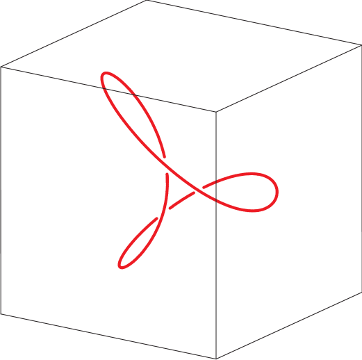
Figure 1: A degree 4 rational curve in $\mathbb{R}\mathbf{P}^{3}$

Specifically, we are interested in enumerative geometry of curves in $X$. For example, we would like to know how many curves of given degree and genus meet given subvarieties of $X$, assuming we expect this number to be finite.

2.1 Parametrized curves and stable maps

2.1.1

A rational curve $C$ in $X=\mathbf{P}^{3}$ like the one in Figure 1 is the image of the Riemann sphere $\mathbf{P}^{1}$ under a map

$$\mathbf{P}^{1}\in z\mapsto f(z)=\left[f_{0}(z):f_{1}(z):f_{2}(z):f_{3}(z)\right]$$ (1)

given in homogeneous coordinates by polynomials $f_{i}$ of degree $d$. Modulo reparameterization of $\mathbf{P}^{1}$, this leaves $4d$ complex parameters for $C$.

To pass through a point in a threefold is a codimension 2 condition on $C$. We, therefore, expect that finitely many degree $d$ rational curves will meet $2d$ points in general position. For example, there is obviously a unique line through two points. Similarly, since any conic lies in a plane, there will be none such passing through 4 generic points. In general, the number of degree $d=1,2,\dots$ rational curves through $2d$ general points of $\mathbf{P}^{3}$ equals

$$1,0,1,4,105,2576,122129,\dots\,,$$

see for example [8, 12] on how to do such computations.

An important ingredient is a compactification of the space of maps (1) to the moduli space of stable maps, introduced by Kontsevich. The domain of a stable map need not be irreducible, it may sprout off additional $\mathbf{P}^{1}$’s like in the case of a smooth conic degenerating to a union of two lines.

2.1.2

In general, the moduli spaces $\overline{\mathcal{M}}_{g,n}(X,\beta)$ of pointed stable maps to $X$ (where $X$ may be of any dimension) consist of data

$$(C,p_{1},\dots,p_{n},f)$$

where $C$ is a complete curve of arithmetic genus $g$ with at worst nodal singularities, $p_{1},\dots,p_{n}$ are smooth marked points of $C$, and $f:C\to X$ is an algebraic map of given degree

$$\beta=f_{*}([C])\in H_{2}(X)\,.$$

Two such objects are identified if they differ by a reparameterization of the domain. One further requirement is that the group of automorphisms (that is, self-isomorphisms) should be finite; this is the stability condition.

2.1.3

The space $\overline{\mathcal{M}}_{g,n}(X,\beta)$ carries a canonical virtual fundamental class [3, 4, 26] of dimension

$$\operatorname{vir\,\,dim}\overline{\mathcal{M}}_{g,n}(X,\beta)=-\beta\cdot K_{X}+(g-1)(3-\dim X)+n\,,$$ (2)

where $K_{X}$ is the canonical class of $X$. The Gromov-Witten invariants of $X$ are defined as intersections of cohomology classes on $\overline{\mathcal{M}}_{g,n}(X,\beta)$ defined by conditions we impose on $f$ (e.g.  by constraining the images $f(p_{i})$ of the marked points) against the virtual fundamental class. In exceptionally good cases, for example when $X=\mathbf{P}^{3}$ and $g=0$, the virtual fundamental class is the usual fundamental class.

Even for $X=\mathbf{P}^{3}$, the situation with higher genus curves is considerably more involved, both in foundational aspects as well as in combinatorial complexity. It is, therefore, remarkable that conjectural correspondence with Donaldson-Thomas theory, to be described momentarily, gives all-genera fixed-degree answers with finite amount of computation.

2.2 Equations of curves and Hilbert scheme

Instead of giving a parameterization, one can describe algebraic curves $C\subset X$ by their equations.

2.2.1

Concretely, if $X\subset\mathbf{P}^{N}$ for some $N$ and $[x_{0}:x_{1}:\dots:x_{N}]$ are homogeneous coordinates on $\mathbf{P}^{N}$ then homogeneous polynomials $f$ vanishing on $C$ form a graded ideal

$$I(C)\subset\mathbb{C}[x_{0},\dots,x_{N}]\,,$$

containing the ideal $I(X)$ of $X$. This ideal is what replaces parametrization of $C$ in the world of equations. For example, the curve in Figure 1 is cut out (that is, its ideal is generated) by one quadratic and 3 cubic equations.

2.2.2

Let $I(C)_{k}\subset\mathbb{C}[x_{0},\dots,x_{N}]_{k}$ denote subspaces formed by polynomials of degree $k$. The codimension of $I(C)_{k}$ is the number of linearly independent degree $k$ polynomials on $C$. By Hilbert’s theorem,

$$\operatorname{codim}I(C)_{k}=(\beta\cdot h)\,k+\chi(\mathcal{O}_{C})\,,\quad k\gg 0\,,$$ (3)

where $\beta\in H_{2}(X)$ is the class of $C$ and $h$ is the hyperplane class induced from the ambient $\mathbf{P}^{N}$. The number

$$\chi(\mathcal{O}_{C})=\dim H^{0}(C,\mathcal{O}_{C})-\dim H^{1}(C,\mathcal{O}_{C})$$

is the holomorphic Euler characteristic of $C$. By definition, $g=1-\chi$ is the arithmetic genus of $C$.

It is easy to see that $C$ is uniquely determined by any $I(C)_{k}$ provided $k\gg 0$. A natural parameter space for ideals $I$ with given Hilbert function (3) is the Hilbert scheme $\operatorname{Hilb}(X;\beta,\chi)$ constructed by Grothendieck. It is defined by certain natural equations in the Grassmannian of all possible linear subspaces $I_{k}\subset\mathbb{C}[x_{0},\dots,x_{N}]_{k}$ of given codimension (3).

2.2.3

While $\operatorname{Hilb}(X;\beta,\chi)$ and $\overline{\mathcal{M}}_{g,n}(X,\beta)$ play the same role of a compact parameter space in the world of equations and parameterizations, respectively, it should be stressed that there is no direct geometric relation between the two. This is most apparent in the case $\beta=0$. In degree $0$ case, the stable map moduli spaces become essentially Deligne-Mumford spaces of stable curves — very nice and well-understood varieties. The Hilbert scheme of points in a $3$-fold $X$, by contrast, seems very complicated. Even the number of its irreducible components, or their dimensions, is not known.

2.2.4

All of what we said so far about the Hilbert scheme applied very generally, in any dimension. The case of curves in a 3-fold, however, is special: in this case $\operatorname{Hilb}(X;\beta,\chi)$ carries a virtual fundamental class constructed by R. Thomas [44]. The technically important thing about 3-folds is that Serre duality limits the number of interesting $\operatorname{Ext}^{i}$-group from an ideal sheaf to itself to just $i=1,2$. From (2) we see that the case $\dim X=3$ is special for Gromov-Witten theory, too. In fact, we have

$$\operatorname{vir\,\,dim}\operatorname{Hilb}(X;\beta,\chi)=\operatorname{vir\,\,dim}\overline{\mathcal{M}}_{g}(X,\beta)=-\beta\cdot K_{X}\,.$$ (4)

As we will see in the next section, it is very fortunate that this dimension depends only on $\beta$.

2.3 Gromov-Witten and Donaldson-Thomas invariants

Let $\beta\in H_{2}(X)$ be such that $-\beta\cdot K_{X}\geq 0$. Let $\gamma_{1},\dots,\gamma_{n}\in H_{*}(X)$ be a collection of cycles in $X$ such that

$$\sum(\operatorname{codim}\gamma_{i}-1)=-\beta\cdot K_{X}\,.$$

By the dimension formula (4), the virtual number of degree $\beta$ curves of some fixed genus meeting all of $\gamma_{i}$’s is expected to be finite.

The precise technical definition of this virtual number is different for stable maps and the Hilbert scheme.

2.3.1

On the stable maps side, we can use marked points $p_{i}$ to say “curve meets $\gamma_{i}$” in the language of cohomology. Namely, imposing the condition $f(p_{i})\in\gamma_{i}$ can be interpreted as pulling back the Poincaré dual class $\gamma_{i}^{\vee}$ via the evaluation map

$$\operatorname{ev}_{i}:(C,p_{1},\dots,p_{n},f)\mapsto f(p_{i})\,.$$ (5)

The Gromov-Witten invariants are defined by

$$\left\langle\gamma_{1},\dots,\gamma_{n}\right\rangle^{GW}_{\beta,g}=\int_{\left[\overline{\mathcal{M}}_{g,n}(X,\beta)^{\bullet}\right]_{vir}}\prod_{i=1}^{n}\operatorname{ev}_{i}^{*}\left(\gamma_{i}^{\vee}\right)\,.$$ (6)

The bullet here stands for moduli space with possibly disconnected domain and $[\quad]_{vir}$ is its virtual fundamental class. The disconnected theory contains, of course, the same information as the connected one, but has slightly better formal properties. Most importantly, since connected curves don’t form a component of the Hilbert scheme, we prefer to work with possibly disconnected curves on the Gromov-Witten side as well.

2.3.2

On the Hilbert scheme side, instead of marked points, it is natural to use characteristic classes of the universal ideal sheaf

$$\mathcal{I}\to\operatorname{Hilb}(X)\times X\,,$$

which has the property that for any point $I\in\operatorname{Hilb}(X)$, the restriction of $\mathcal{I}$ to $I\times X\cong X$ is $I$ itself. We have $c_{1}(\mathcal{I})=0$ and

$$c_{2}(\mathcal{I})\in H^{2}\left(\operatorname{Hilb}(X)\times X\right)$$

can be interpreted as the class of locus

$$\{(I,\text{point of the curve defined by $I$})\}\subset\operatorname{Hilb}(X)\times X\,.$$

The class of curves $I\in\operatorname{Hilb}(X)$ meeting $\gamma\in H_{*}(X)$ can be described as the coefficient of $\gamma^{\vee}$ in the Künneth decomposition of $c_{2}(\mathcal{I})$. We denote this component by

$$c_{2}(\gamma)\in H^{\operatorname{codim}\gamma-1}(\operatorname{Hilb}(X))$$

and define

$$\left\langle\gamma_{1},\dots,\gamma_{n}\right\rangle^{DT}_{\beta,\chi}=\int_{\left[\operatorname{Hilb}(X;\beta,\chi)\right]_{vir}}\prod_{i=1}^{n}c_{2}(\gamma_{i})\,.$$ (7)

We call these numbers the Donaldson-Thomas invariants of $X$.

2.4 Main conjecture

2.4.1

As already pointed out, there is no reason for the corresponding invariants (6) and (7) to agree and, in fact, they don’t. For one thing, the moduli spaces are empty and, hence, integrals vanish if $g,\chi\ll 0$, which goes in the opposite directions via $\chi=1-g$. Also, the Donaldson-Thomas invariants are integers while the Gromov-Witten invariants are typically fractions (because stable maps can have finite automorphisms). However, a conjecture proposed in [30] equates natural generating functions for the two kinds of invariants after a nontrivial change of variables.

2.4.2

Concretely, set

$$Z_{GW}(\gamma_{1},\dots,\gamma_{n};u)_{\beta}=\sum_{g}u^{2g-2}\,\left\langle\gamma_{1},\dots,\gamma_{n}\right\rangle^{GW}_{\beta,g}$$

and define the reduced partition function by

$$Z^{\prime}_{GW}(\gamma;u)_{\beta}=Z_{GW}(\gamma;u)_{\beta}\big{/}Z_{GW}(\varnothing;u)_{0}\,.$$

This reduced partition function counts maps without collapsed connected components. The degree zero function $Z_{GW}(\varnothing;u)_{0}$ is known explicitly for any 3-fold $X$ by the results of [11], see below. Define $Z_{DT}(\gamma;q)_{\beta}$ and its reduced version by the same formula, with $q^{\chi}$ replacing $u^{2g-2}$.

Conjecture 1.

The reduced Donaldson-Thomas partition function $Z^{\prime}_{DT}(\gamma;q)_{\beta}$ is a rational function of $q$. The change of variables

$$\boxed{q=-e^{iu}}$$

relates it to the Gromov-Witten partition functions

$$(-iu)^{-\operatorname{vir\,\,dim}}Z^{\prime}_{GW}(\gamma;u)_{\beta}=(-q)^{-\operatorname{vir\,\,dim}/2}Z^{\prime}_{DT}(\gamma;q)_{\beta}\,,$$

where $\operatorname{vir\,\,dim}=-\beta\cdot K_{X}$ is the virtual dimension.

2.4.3

Conjecture 1 has been established when $X$ is either a local curve, that is, an arbitrary rank 2 bundle over a smooth curve [42] or the total space of canonical bundle over a smooth toric surface [30, 28]. In the local curve case, equivariant theory is needed [6]. In my opinion, this provides substantial evidence for the “GW=DT” correspondence.

2.4.4

Conjecture 1 is actually a special case of more general conjectures proposed in [30] that extend the GW/DT correspondence to the relative context and descendent invariants. On the Gromov-Witten side, the descendent insertions are defined by

$$\tau_{k}(\gamma_{i})=\operatorname{ev}_{i}^{*}(\gamma_{i}^{\vee})\,\psi_{i}^{k}\in H^{\operatorname{codim}\gamma_{i}+k}(\overline{\mathcal{M}}_{g,n}(X;\beta))\,,$$

where $\psi_{i}$ is the 1st Chern class of the line bundle $L_{i}$ over $\overline{\mathcal{M}}_{g,n}(X;\beta)$ with fiber the cotangent line $T^{*}_{p_{i}}C$ to the curve $C$ at the marked point $p_{i}$. These should correspond to Künneth components of characteristic classes of the universal sheaf $\mathcal{I}$. For example, we conjecture that

$$\tau_{k}(pt)\xrightarrow{\quad\textup{GW=DT}\quad}(-1)^{k+1}\operatorname{ch}_{k+2}(pt)\,,$$

provided $\operatorname{codim}\gamma_{i}>0$ for all other insertions. Here

$$\operatorname{ch}_{k+2}(\mathcal{I})\in H^{k+2}(\operatorname{Hilb}(X)\times X)$$

are the components of the Chern character of $\mathcal{I}$ and $\operatorname{ch}_{k+2}(pt)$ are the coefficient of $pt^{\vee}=1\in H^{*}(X)$ in their Künneth decomposition.

2.4.5

In the degree $0$ case, which is left out by Conjecture 1, we expect the following simple answer which depends only on characteristic numbers of $X$. Denote the Chern classes of $TX$ by $c_{i}$ and let

$$M(q)=\prod_{n>0}(1-q^{n})^{-n}$$ (8)

be the McMahon function.

Conjecture 2.

$\displaystyle\quad Z_{DT}(X,q)_{0}=M(-q)^{\int_{X}(c_{3}-c_{1}c_{2})}\,.$

This conjecture has been proven for a large class of 3-folds including all toric ones [30].

Comparing the asymptotic expansion

$$\ln M(e^{-u})\sim\sum_{g=0}^{\infty}\frac{\zeta(3-2g)\zeta(1-2g)}{(2g-2)!}\,u^{2g-2}\,,\quad u\to+0\,.$$ (9)

in which the singular $g=1$ term is understood as the second term in

$$\frac{\zeta(3-2g)\zeta(1-2g)}{(2g-2)!}\,u^{2g-2}=\frac{1}{24}\frac{1}{g-1}+\left(\frac{1}{12}\ln u+\zeta^{\prime}(-1)\right)+O(g-1)\,,$$

to evaluation of $Z_{GW}(X,u)_{0}$ obtained in [11], we find

$$\ln Z_{DT}(X,-e^{iu})_{0}\sim\dots+2\ln Z_{GW}(X,u)_{0}\,,$$

where dots stand for singular or constant terms in the asymptotic expansion. There are some plausible explanations for the unexpected factor of $2$ in this formula, but none convincing enough to be presented here.

McMahon’s discovery was that the function $M(q)$ is the generating function for 3-dimensional partitions. We will see momentarily how 3-dimensional partitions arise in Donaldson-Thomas theory.

3 Random surfaces

3.1 Localization and dissolving crystals

3.1.1

For the rest of this lecture, we will assume that $X$ is a smooth toric $3$-fold, such as $\mathbf{P}^{3}$ or $(\mathbf{P}^{1})^{3}$. By definition, this means, that the torus $\mathbf{T}=(\mathbb{C}^{*})^{3}$ acts on $X$ with an open orbit. Since anything that acts on $X$ naturally acts on both $\overline{\mathcal{M}}_{g,n}(X;\beta)$ and $\operatorname{Hilb}(X;\beta,\chi)$, localization in $\mathbf{T}$-equivariant cohomology [2] can be used to compute intersections on these moduli spaces, see [10, 23, 13].

Localization reduces intersection computations to certain integrals over the loci of $\mathbf{T}$-fixed points. On the Gromov-Witten side, these fixed loci are, essentially, moduli spaces of curves and the integrals in question are the so-called Hodge integrals. While any fixed-genus Hodge integral can, in principle, be evaluated in finite time, a better structural understanding of the totality of these numbers remains an important challenge. By contrast, the $\mathbf{T}$-fixed loci in the Hilbert scheme are isolated points. Together with the conjectural rationality of $Z^{\prime}_{DT}$, this reduces, for fixed degree, the all-genera answer to a finite sum.

3.1.2

It is the localization sum in the Donaldson-Thomas theory that can be interpreted as the partition function of a certain random surface ensemble. The link is provided by the combinatorial geometry of the $\mathbf{T}$-fixed points in the Hilbert scheme, which is standard and will be quickly reviewed now.

3.1.3

As a warm-up, let us start with surfaces instead of $3$-folds and look at the Hilbert scheme $\operatorname{Hilb}(\mathbb{C}^{2};d,n)$ formed by ideals $I\subset\mathbb{C}[x,y]$ such that

$$\operatorname{codim}I_{\leq k}=dk+n\,,\quad k\gg 0\,,$$ (10)

where $I_{\leq k}$ stands for subspace of polynomials of degree $\leq k$. The torus $(\mathbb{C}^{*})^{2}$ acts on $\operatorname{Hilb}(\mathbb{C}^{2};d,n)$ by rescaling $x$ and $y$. The monomials $x^{i}y^{j}$ are eigenvectors of the torus action with distinct eigenvalues. Any torus-fixed linear subspace $I\subset\mathbb{C}[x,y]$ is, therefore, spanned by monomials. Since $I$ is also an ideal, together with any monomial $x^{i}y^{j}$ it contains all monomials $x^{a}y^{b}$ with $a\geq i$ and $b\geq j$.

Figure 2: A typical monomial ideal $I\subset\mathbb{C}[x,y]$.

See Figure 2 for an image of a typical torus-fixed ideal $I$. Monomials in the ideal $I$ are shaded gray; the generators of $I$ are circled. Monomials not in $I$ form a shape similar to the diagram of a partition, except that it has some infinite rows and columns. The total width of these infinite rows and columns ($2$, in this example) is the degree $d$ in (10). The constant term $\chi$ ($=9$ here) can be interpreted as the “renormalized area” of this infinite diagram.

3.1.4

For $\operatorname{Hilb}(\mathbb{C}^{3};d,\chi)$, the description of $\mathbf{T}$-fixed points $I$ is similar, but now in terms of 3-dimensional partitions, with possibly infinite legs along the coordinate axes, see Figure 3. The 2D partitions $\lambda_{1},\lambda_{2},\lambda_{3}$, on which the infinite legs end, describe the nonreduced structure of $I$ along the coordinate axes. The degree

$$d=|\lambda_{1}|+|\lambda_{2}|+|\lambda_{3}|$$

is the total cross-section of the infinite legs; the number $\chi$ is the renormalized volume of this 3D partition.

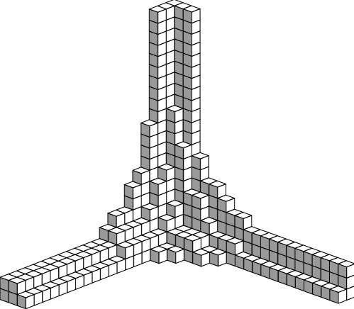
Figure 3: A monomial ideal in $\operatorname{Hilb}(C^{3};d,\chi)$

A general projective toric $X$ corresponds to lattice polytope $\Delta_{X}$, with vertices corresponding to $\mathbf{T}$-fixed points, edges — to $\mathbf{T}$-invariants $\mathbf{P}^{1}$’s et cetera. For example, $(\mathbf{P}^{1})^{3}$ and $\mathbf{P}^{3}$ corresponds to a cube and simplex, respectively. To specify a $\mathbf{T}$-fixed point in $\operatorname{Hilb}(X;\beta,\chi)$, we place a 3D partition at every vertex of $\Delta_{X}$. These 3D partition may have infinite legs along the edges of $\Delta_{X}$; we require that these legs glue in an obvious way, see Figure 4, left half. We have

$$\beta=\sum_{\textup{edges $E$}}|\lambda_{E}|\,\left[E\right]\in H_{2}(X)\,,$$

where $[E]$ is the class of the $\mathbf{T}$-invariant $\mathbf{P}^{1}$ corresponding to the edge $E$ and $\lambda_{E}$ is cross-section profile along $E$. The number $\chi$ is the renormalized volume of this assembly of 3D partitions.

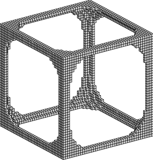
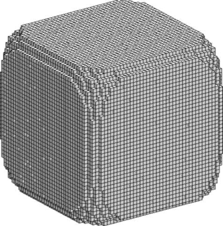
Figure 4: A $\mathbf{T}$-fixed point in $\operatorname{Hilb}((\mathbf{P}^{1})^{3};\beta,\chi)$

Note that the edge lengths do not have any intrinsic meaning in Figure 4; formally, they have to be viewed as infinitely long. It is an interesting problem to construct a generalization of Donaldson-Thomas theory in which the edge lengths will play a role. This should involve doubling of the degree parameters in the theory.

The right half of Figure 4 shows the complement of the 3D partition structure on the left. Note that it is highly reminiscent of a partially dissolved cubic crystal — some atoms are missing from the corners and along the edges. So, at least as far as the index set is concerned, the localization sum in Donaldson-Thomas theory of $X$ has the shape of a partition function in a random surface model, the surface being the surface of the dissolving crystal. We now move on to the computation of localization weight.

3.2 Equivariant vertex

The weight of a $\mathbf{T}$-fixed point $I\in\operatorname{Hilb}(X;\beta,\chi)$ in the virtual localization formula for Donaldson-Thomas invariants was computed in [30]. Here, for simplicity, we focus on the case $X=\mathbb{C}^{3}$ and $\beta=0$, that is, on the case of a single 3D partition without infinite legs. The general case is parallel.

3.2.1

Let $I_{\pi}\in\operatorname{Hilb}(\mathbb{C}^{3};0,\chi)$ be a monomial ideal corresponding to a 3D partition $\pi\subset\mathbb{Z}_{\geq 0}^{3}$. Let $C_{\pi}\subset\mathbb{Z}_{\geq 0}^{3}$ denote the complement of $\pi$; we view the elements of $C_{\pi}$ as the atoms that remain in the crystal.

Let $z\in\mathbb{C}^{*}\subset\mathbf{T}$ act on the coordinates in $\mathbb{C}^{3}$ by

$$z\cdot(x_{1},x_{2},x_{3})=(z^{t_{1}}x_{1},z^{t_{2}}x_{2},z^{t_{3}}x_{3})\,.$$

The localization weight $\mathsf{w}(\pi)$ of $I_{\pi}$ will be a rational function of the parameters $t_{i}$. Let $T$ be the linear function taking value

$$T(\textup{\char 114})=t_{1}a_{1}+t_{2}a_{2}+t_{3}a_{3}\,.$$

on a box $\textup{\char 114}=(a_{1},a_{2},a_{3})\in\mathbb{Z}_{\geq 0}^{3}$. For a pair of boxes $\textup{\char 114}_{1}$ and $\textup{\char 114}_{2}$, we define

$$U(\textup{\char 114}_{1},\textup{\char 114}_{2})=\frac{\delta T(\delta T+t_{1}+t_{2})(\delta T+t_{1}+t_{3})(\delta T+t_{2}+t_{3})}{(\delta T+t_{1})(\delta T+t_{2})(\delta T+t_{3})(\delta T+t_{1}+t_{2}+t_{3})}\,,$$

where

$$\delta T=T(\textup{\char 114}_{1})-T(\textup{\char 114}_{2})\,.$$

Recall that $\chi$ is the number of missing atoms. We would have liked to define $\mathsf{w}(\pi)$ by

$$\mathsf{w}(\pi)\textup{ ``$=$'' }(-q)^{\chi}\prod_{\textup{\char 114}_{1},\textup{\char 114}_{2}\in\textup{ crystal $C_{\pi}$}}U(\textup{\char 114}_{1},\textup{\char 114}_{2})\,,$$ (11)

which has a standard grand-canonical Gibbs form with $(-q)$ being the fugacity and

$$-\log U(\textup{\char 114}_{1},\textup{\char 114}_{2})\,U(\textup{\char 114}_{2},\textup{\char 114}_{1})$$

being the (translation-invariant) interaction energy between the atoms in positions $\textup{\char 114}_{1}$ and $\textup{\char 114}_{2}$.

3.2.2

Since the product (11) is not even close to being well-defined or convergent, the following regularization is required. Define

$$R_{\pi}(z)=\textup{trace of $z$ acting on $I_{\pi}$}=\sum_{\textup{\char 114}\in C_{\pi}}z^{T(\textup{\char 114})}\,,$$ (12)

This can be viewed as a generating function of the set $C_{\pi}$. One checks that for any 3D partition $\pi$

$$\mathsf{V}_{\pi}(z)=-\frac{R_{\pi}(z)\,R_{\pi}(z^{-1})}{R_{\varnothing}(z^{-1})}+R_{\varnothing}(z)$$ (13)

is a Laurent polynomials in $z^{t_{i}}$, that is, it has the form

$$\mathsf{V}_{\pi}(z)=\sum_{a\in\mathbb{Z}^{3}}v_{\pi}(a)\,z^{T(a)}\,,\quad v_{\pi}(a)\in\mathbb{Z}\,,$$

where the sum is finite, that is, $v_{\pi}(a)=0$ for all but finitely many $a$. We define the equivariant vertex measure of a 3D partition $\pi$ by

$$\mathsf{w}(\pi)=q^{\chi}\prod_{a\in\mathbb{Z}}T(a)^{-v_{\pi}(a)}\,.$$

Note that a naive expansion of the $R_{\pi}(z)\,R_{\pi}(z^{-1})$ product in (13) leads to the infinite product in (11).

3.2.3

It is a theorem from [30] that the virtual fundamental class of the Hilbert scheme restricts to the $\mathbf{T}$-fixed point $I_{\pi}$ as follows:

$$q^{\chi}\left[\operatorname{Hilb}(\mathbb{C}^{3};0,\chi)\right]_{vir}\bigg{|}_{I_{\pi}}=\mathsf{w}(\pi)\,.$$

3.2.4

One special case worth noting is when

$$t_{1}+t_{2}+t_{3}=0\,.$$ (14)

In this case

$$U(\textup{\char 114}_{1},\textup{\char 114}_{2})\,U(\textup{\char 114}_{2},\textup{\char 114}_{1})=1$$

and the equivariant vertex measure $\mathsf{w}$ becomes uniform on partitions of fixed size. Condition (14) is the Calabi-Yau condition, it means restriction to the subtorus in $\mathbf{T}$ preserving the holomorphic $3$-form

$$\Omega=dx_{1}\wedge dx_{2}\wedge dx_{3}$$

on $\mathbb{C}^{3}$. This explains why the McMahon function (8) appears in Donaldson-Thomas theory.

For general $t_{i}$, the analog of McMahon’s identity is the following formula proven in [30]

$$\sum_{\pi}\mathsf{w}(\pi)=M(-q)^{-\tfrac{(t_{1}+t_{2})(t_{1}+t_{3})(t_{2}+t_{3})}{t_{1}t_{2}t_{3}}}\,.$$ (15)

This formula implies Conjecture 2 for any toric $3$-fold $X$.

3.2.5

If $\pi$ has infinite legs, additional counterterms are needed in (13) to make it finite and the measure $\mathsf{w}(\pi)$ well-defined [30]. The equivariant vertex is a function of 3 partitions $\lambda,\mu,\nu$ defined by

$$\mathsf{W}(\lambda,\mu,\nu)=\sum_{\textup{$\pi$ ending on $\lambda,\mu,\nu$}}\mathsf{w}(\pi)\,.$$ (16)

This function, which is the main building block in localization formula for Donaldson-Thomas invariants, is, in general, rather intricate. Conjecturally it is related to general triple Hodge integrals. In the Calabi-Yau case (14) it specializes to the topological vertex [1, 43], which has an expression in terms of Schur functions. The conjectural relation to Hodge integrals is proven in the one-leg case [42]. In the much simpler Calabi-Yau case, it is known in the two-leg case, see [28] and also [27, 40, 25].

3.2.6

Conjecture 1 relates the Donaldson-Thomas partition function $Z_{DT}$, which we just interpreted as the partition function of a certain dissolving crystal model, to the the Gromov-Witten partition function via the substitution

$$-q=e^{iu}\,.$$

This means that the asymptotic expansion of the free energy $\ln Z_{DT}$ in the thermodynamic limit

$$-q=\textup{fugacity}\to 1$$

gives a genus-by-genus count of connected curves in Gromov-Witten theory. Letting $q\to-1$ does corresponds to letting the energy cost of removal of an atom from the crystal go to zero. As a result, the expected number of removed atoms

$$\left\langle|\pi|\right\rangle_{\mathsf{w}}\,\overset{\textup{def}}{=}\,\frac{\sum\mathsf{w}(\pi)\,|\pi|}{\sum\mathsf{w}(\pi)}\sim\frac{(t_{1}+t_{2})(t_{1}+t_{3})(t_{2}+t_{3})}{t_{1}t_{2}t_{3}}\,\frac{2\zeta(3)}{\ln(-q)^{3}}\,,$$ (17)

diverges.

In general, the words “thermodynamic limit” have to be taken with a grain of salt since $\mathsf{w}$ is not necessarily a positive measure. However, for example in the uniform measure case (14) it is positive for $-q\in(0,1)$. After scaling by $-\ln(-q)$ in every direction, a macroscopic limit shape emerges. A simulation of the limit shape can be seen in Figure 5.

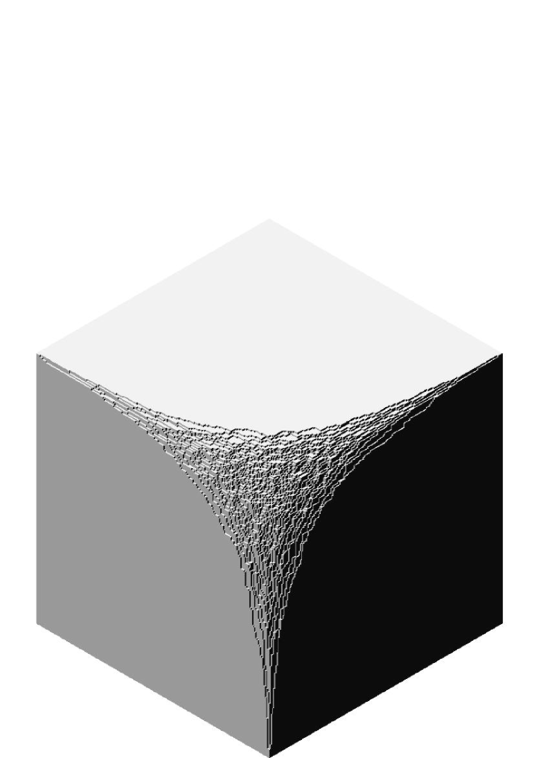
Figure 5: A random 3D partition of a large number

The limit shape dominates the partition function $Z_{DT}$. The Gromov-Witten partition function $Z_{GW}$ is determined by the fluctuations around the limit shape.

3.2.7

The limit shape of a uniformly random 3D partition of a large number, first determined in [7], is, as it turns out, nothing but the so-called Ronkin function of the simplest plane curve

$$z+w=1\,,$$ (18)

see [19] for a much more general result.

Surprisingly (or not ?) the straight line (18) is essentially the Hori-Vafa mirror [14] of $\mathbb{C}^{3}$, see e.g. Section 2.5 in [1]. The mirror geometry thus can be interpreted as the limit shape in the localization formula for the original counting problem.

This phenomenon was first observed in [34] in the context of supersymmetric gauge theories on $\mathbb{R}^{4}$. Namely, in [34] the Seiberg-Witten curve was identified with the limit shape in a certain random partition ensemble originating from localization on the instanton moduli spaces [33]. This limit shape interpretation gave a a gauge-theoretic derivation of the Seiberg-Witten prepotential, see [34] and also [32] for a different approach. Via a physical procedure called geometric engineering, supersymmetric gauge theories correspond to Gromov-Witten theory of certain noncompact toric Calabi-Yau threefolds $X$, see for example [17, 15].

For toric Calabi-Yau $X$, the random surface model can be viewed as a very degenerate limit of the planar dimer model. There is general method for finding limit shapes in the dimer model, which often gives essentially algebraic answers [18]. In particular, it reproduces the Hori-Vafa mirrors of toric Calabi-Yau 3-folds [20]. It would be extremely interesting to extend the

“mirror geometry = limit shape”

philosophy to a more general class of varieties and/or theories.

3.2.8

A natural set of observables to average against the equivariant vertex measure is provided by the characteristic classes of the universal sheaf $\mathcal{I}$, see Section 2.3.2, in particular, by the components $\operatorname{ch}_{k}(\mathcal{I})$ of its Chern character. The restriction $\operatorname{ch}_{k}(\pi)$ of $\operatorname{ch}_{k}(\mathcal{I})$ to a fixed point $I_{\pi}\in\operatorname{Hilb}(\mathbb{C}^{3};0,\chi)$ is determined in terms of the generating function (12) by

$$\sum_{k}\alpha^{k}\,\operatorname{ch}_{k}(\pi)=\frac{R_{\pi}(e^{\alpha})}{R_{\varnothing}(e^{\alpha})}\,.$$

The algebra generated by $\operatorname{ch}_{k}(\pi)$ can be viewed as the algebra of symmetric polynomials in $\pi$; this is a 3-dimensional analog of the algebra introduced in [21].

We have $\operatorname{ch}_{1}(\pi)=0$, $\operatorname{ch}_{2}(\pi)=\textup{degree}=0$, and

$$\operatorname{ch}_{3}(\pi)=t_{1}t_{2}t_{3}|\pi|\,,$$

so from (15) we get the evaluation

$$\langle\operatorname{ch}_{3}(\pi)\rangle_{\mathsf{w}}=-(t_{1}+t_{2})(t_{1}+t_{3})(t_{2}+t_{3})\,E_{3}(-q)\,.$$

Here $E_{2k+1}$ are the following “odd weight” analogs of the classical Eisenstein series

$$E_{2k+1}(q)=\sum_{n}q^{n}\sum_{d|n}d^{2k}\,,\quad k=1,2,\dots\,.$$ (19)

One further computes, for example,

$$\langle\operatorname{ch}_{4}(\pi)\rangle_{\mathsf{w}}=-\frac{1}{2}\,(t_{1}+t_{2})(t_{1}+t_{3})(t_{2}+t_{3})(t_{1}+t_{2}+t_{3})\,q\frac{d}{dq}E_{3}(-q)\,,$$

and the natural conjecture is that all $\langle\operatorname{ch}_{k}(\pi)\rangle_{\mathsf{w}}$ belong to the differential algebra generated by the functions (19) and the operator $q\frac{d}{dq}$. A similar statement for ordinary 2D partitions and usual even weight Eisenstein series was proven in [5].

Note, in particular, this conjecture implies that the “thermodynamic” asymptotics of $\langle\operatorname{ch}_{k}(\pi)\rangle_{\mathsf{w}}$ as $q\to-1$ is completely determined by the first few coefficients of its “low temperature” $q$-expansion. For a complete $3$-fold $X$, a similar property is implied by the conjectural rationality of the reduced partition function $Z^{\prime}_{DT}$.

3.2.9

Recall that on the Gromov-Witten side, the observables $\operatorname{ch}_{k}(\mathcal{I})$ are supposed to correspond to descendent invariants. While working out an exact match, especially in the equivariant theory, remains an open problem (see the discussion in [30]), there is one case that we understand well.

Let $X=\mathbf{P}^{1}\times\mathbb{C}^{2}$ and let $\beta$ be $d$ times the class of $\mathbf{P}^{1}\times\{0\}$. Let $\mathbb{C}^{*}$ act on $\mathbb{C}^{2}$ with opposite weights. The $\mathbb{C}^{*}$-equivariant Gromov-Witten theory of $X$ is the Gromov-Witten of $\mathbf{P}^{1}$ with additional insertion of two Chern polynomials of the Hodge bundle. Because of our choice of weights and Mumford’s relation, these Chern polynomials cancel out, leaving us with the Gromov-Witten theory of $\mathbf{P}^{1}$.

A complete description of the Gromov-Witten theory of $\mathbf{P}^{1}$ was obtained in [37, 38, 39]. In particular, we have the following formula for disconnected, degree $d$ descendent invariants of the point class

$$\left\langle\prod\tau_{k_{i}}(pt)\right\rangle_{d}^{\mathbf{P}^{1}}=\sum_{|\lambda|=d}\left(\frac{\dim\lambda}{d!}\right)^{2}\,\prod_{i}\frac{\mathbf{p}_{k_{i}+1}(\lambda)}{(k_{i}+1)!}\,,$$ (20)

where the summation is over partitions $\lambda$ of $d$, $\dim\lambda$ is the dimension of the corresponding representation of the symmetric group, and $\mathbf{p}_{k}$ is the following polynomial of $\lambda$

$$\mathbf{p}_{k}(\lambda) \,=\sum_{i}\left[(\lambda_{i}-i+\tfrac{1}{2})^{k}-(-i+\tfrac{1}{2})^{k}\right]+(1-2^{-k})\zeta(-k)$$

$$\textup{``=''}\sum_{i}(\lambda_{i}-i+\tfrac{1}{2})^{k}\,.$$

Here the first line is the $\zeta$-regularization of the divergent sum in the second line. The weight function in (20) is known as the Plancherel measure on partitions of $d$.

Sums of the form (20) are distinguished discrete analogs of matrix integrals mentioned at the very beginning of the lecture, see e.g. the discussion in [35].

What happens on the Donaldson-Thomas side is that with our choice of torus weights the contribution of most $\mathbf{T}$-fixed points to the localization formula vanishes. The only remaining ones are of the form seen in Figure 6, they are pure edges, that is, cylinders over an ordinary partition $\lambda$.

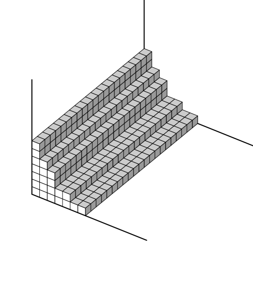
Figure 6: A pure edge

Sure enough, the localization weight of such a pure edge in this case specializes to the Plancherel weight of its cross-section $\lambda$. Also, the restrictions of $\operatorname{ch}_{k}(\mathcal{I})$ to such a fixed point has a simple linear relation to the numbers $\mathbf{p}_{k}(\lambda)$.

It was noticed by several people, in particular in [24, 29], that the sum (20) is closely related to localization expressions in the classical cohomology of the Hilbert scheme of $d$ points in $\mathbb{C}^{2}$. Perhaps the best explanation for this relation is that it is a specialization of the triangle of equivalences in Figure 7, see [41].

Figure 7: Three points of view on curves in $\mathbf{P}^{1}\times\mathbb{C}^{2}$

References

- [1] M. Aganagic, A. Klemm, M. Marino, C. Vafa, The topological vertex, hep-th/0305132.
- [2] M. Atiyah and R. Bott, The moment map and equivariant cohomology, Topology 23 (1984), 1-28.
- [3] K. Behrend, Gromov-Witten invariants in algebraic geometry, Invent. Math. 127 (1997), 601–617.
- [4] K. Behrend and B. Fantechi, The intrinsic normal cone, Invent. Math. 128 (1997), 45–88.
- [5] S. Bloch and A. Okounkov, The Character of the Infinite Wedge Representation, Adv. Math. 149 (2000), no. 1, 1–60.
- [6] J. Bryan and R. Pandharipande, The local Gromov-Witten theory of curves, math.AG/0411037.
- [7] R. Cerf and R. Kenyon, The low-temperature expansion of the Wulff crystal in the three-dimensional Ising model, Comm. Math. Phys 222 (2001),147-179.
- [8] D. Cox and S. Katz, Mirror symmetry and algebraic geometry, American Mathematical Society, Providence, RI, 1999.
- [9] S. Donaldson and R. Thomas, Gauge theory in higher dimensions, in The geometric universe: science, geometry, and the work of Roger Penrose, S. Huggett et. al eds., Oxford Univ. Press, 1998.
- [10] G. Ellingsrud, S. Strømme, Bott’s formula and enumerative geometry. J. Amer. Math. Soc. 9 (1996), no. 1, 175–193.
- [11] C. Faber and R. Pandharipande, Hodge integrals and Gromov-Witten theory, Invent. Math. 139 (2000), 173-199.
- [12] W. Fulton and R. Pandharipande, Notes on stable maps and quantum cohomology, Algebraic geometry—Santa Cruz 1995, 45–96, Proc. Sympos. Pure Math., 62, Part 2, AMS, Providence, RI, 1997.
- [13] T. Graber and R. Pandharipande, Localization of virtual classes, Invent. Math. 135 (1999), 487–518.
- [14] K. Hori and C. Vafa, Mirror Symmetry, hep-th/0002222.
- [15] A. Iqbal and A.-K. Kashani-Poor, SU(N) Geometries and Topological String Amplitudes, hep-th/0306032.
- [16] A. Iqbal, N. Nekrasov, A. Okounkov, C. Vafa, Quantum Foam and Topological Strings, hep-th/0312022.
- [17] S. Katz, A. Klemm, C. Vafa, Geometric engineering of quantum field theories, Nuclear Phys. B 497 (1997), no. 1-2, 173–195.
- [18] R. Kenyon, A. Okounkov, Limit shapes and complex Burgers equation, in preparation.
- [19] R. Kenyon, A. Okounkov, S. Sheffield, Dimers and Amoebae, math-ph/0311005.
- [20] R. Kenyon, A. Okounkov, C. Vafa, in preparation.
- [21] S. Kerov and G. Olshanski, Polynomial functions on the set of Young diagrams, C. R. Acad. Sci. Paris Sér. I Math., 319, no. 2, 1994, 121–126.
- [22] M. Kontsevich, Intersection theory on the moduli space of curves and the matrix Airy function, Comm. Math. Phys. 147 (1992), 1-23.
- [23] M. Kontsevich, Enumeration of rational curves via torus actions, The moduli space of curves (Texel Island, 1994), 335–368, Progr. Math., 129, Birkh user Boston, Boston, MA, 1995.
- [24] W.-P. Li, Zh. Qin, W. Wang, Hilbert schemes, integrable hierarchies, and Gromov-Witten theory, math.AG/0302211.
- [25] J. Li, C.-C. Liu, K. Liu, J. Zhou , A Mathematical Theory of the Topological Vertex, math.AG/0408426.
- [26] J. Li and G. Tian, Virtual moduli cycles and Gromov-Witten invariants of algebraic varieties, JAMS 11 (1998), 119–174.
- [27] C.-C. Liu, K. Liu, J. Zhou , A Proof of a Conjecture of Marino-Vafa on Hodge Integrals, math.AG/0306434.
- [28] C.-C. Liu, K. Liu, J. Zhou , A Formula of Two-Partition Hodge Integrals, math.AG/0310272.
- [29] A. Losev, A. Marshakov, N. Nekrasov, Small Instantons, Little Strings and Free Fermions, hep-th/0302191.
- [30] D. Maulik, N. Nekrasov, A. Okounkov, and R. Pandharipande, Gromov-Witten theory and Donaldson-Thomas theory, I and II, math.AG/0312059, math.AG/0406092.
- [31] M. Mirzakhani, Weil-Petersson volumes and intersection theory on the moduli spaces of curves, available from http://abel.math.harvard.edu/mirzak/.
- [32] H. Nakajima, K. Yoshioka, Instanton counting on blowup, I, math.AG/0306198.
- [33] N. Nekrasov, Seiberg-Witten Prepotential From Instanton Counting, hep-th/0206161.
- [34] N. Nekrasov and A. Okounkov, Seiberg-Witten Theory and Random Partitions, hep-th/0306238.
- [35] A. Okounkov, The uses of random partitions, math-ph/0309015.
- [36] A. Okounkov and R. Pandharipande, Gromov-Witten theory, Hurwitz numbers, and matrix models, I, math.AG/0101147.
- [37] A. Okounkov and R. Pandharipande, Gromov-Witten theory, Hurwitz theory, and completed cycles, math.AG/0204305.
- [38] A. Okounkov and R. Pandharipande, The equivariant Gromov-Witten theory of , math.AG/0207233.
- [39] A. Okounkov and R. Pandharipande, Virasoro constraints for target curves, math.AG/0308097.
- [40] A. Okounkov and R. Pandharipande, Hodge integrals and invariants of the unknot, Geom. Topol. 8(2004), 675-699.
- [41] A. Okounkov and R. Pandharipande, Quantum cohomology of the Hilbert scheme of points in the plane, math.AG/0411210.
- [42] A. Okounkov and R. Pandharipande, Gromov-Witten/Donaldson-Thomas correspondence for local curves, in preparation.
- [43] A. Okounkov, N. Reshetikhin, and C. Vafa, Quantum Calabi-Yau and classical crystals, hep-th/0310061.
- [44] R. Thomas, A holomorphic Casson invariant for Calabi-Yau 3-folds, and bundles on K3 fibrations, JDG 54 (2000), 367–438.
- [45] E. Witten, Two dimensional gravity and intersection theory on moduli space, Surveys in Diff. Geom. 1 (1991), 243-310.