Constant connections,
quantum holonomies and
the Goldman bracket

Abstract

In the context of $2+1$–dimensional quantum gravity with negative cosmological constant and topology $\mathbb{R}\!\times\!T^{2}$, constant matrix–valued connections generate a $q$–deformed representation of the fundamental group, and signed area phases relate the quantum matrices assigned to homotopic loops. Some features of the resulting quantum geometry are explored, and as a consequence a quantum version of the Goldman bracket is obtained.

1 Introduction

Holonomy quantization in the context of $2+1$–dimensional gravity with topology $\mathbb{R}\!\times\!T^{2}$ and negative cosmological constant $\Lambda$ has been discussed from a variety of points of view, e.g. in terms of traced holonomies in [1, 2], and in terms of the holonomy matrices themselves [3, 4]. For further background see [5] and for a comparison with the second–order ADM approach see [6].

In previous articles [3, 4, 7] we have studied $SL(2,\mathbb{R})$ holonomy matrices $U_{1},\,U_{2}$ of the diagonal form

$$U_{i}=\left(\begin{array}[]{clcr}e^{{r_{i}}}&0\\ 0&e^{-{r_{i}}}\end{array}\right)\quad i=1,2$$ (1)

considered as holonomies of the connection integrated along cycles $\gamma_{1},\gamma_{2}$ which generate the fundamental group of the torus, subject to the relation

$$\gamma_{1}\cdot\gamma_{2}\cdot\gamma_{1}^{-1}\cdot\gamma_{2}^{-1}={\mathbb{I}}.$$ (2)

One of the reasons for studying matrices of the type (1) is that their gauge-invariant (normalized) traces $~{}T_{1}^{\pm}=\frac{1}{2}TrU_{1}^{\pm}$ and $T_{2}^{\pm}=\frac{1}{2}TrU_{2}^{\pm}$ appear in $2+1$–dimensional gravity in various guises. In first–order holonomy quantization [1, 2] they satisfy the non–linear Poisson bracket algebra

$$\{T_{1}^{\pm},T_{2}^{\pm}\}=\mp\frac{\sqrt{-\Lambda}}{4}(T_{12}^{\pm}-T_{1}^{\pm}T_{2}^{\pm}),$$ (3)

where in (3) the $\pm$ refer to the two copies (real and independent) of $\hbox{SL}(2,\mathbb{R})$ in the isomorphism $\hbox{SO}(2,2)\cong\hbox{SL}(2,\mathbb{R})\otimes\hbox{SL}(2,\mathbb{R})$, and $T_{12}^{\pm}=\frac{1}{2}Tr(U_{1}^{\pm}U_{2}^{\pm})$ corresponds to the loop $\gamma_{1}\cdot\gamma_{2}$. This loop has intersection number $-1$ with $\gamma_{1}$ and $+1$ with $\gamma_{2}$ (we assume the intersection number between $\gamma_{1}$ and $\gamma_{2}$ is $+1$.)

The traced holonomies of (3) can be represented classically as

$$T_{1}^{\pm}=\cosh r_{1}^{\pm},\quad T_{2}^{\pm}=\cosh r_{2}^{\pm},\quad T_{12}^{\pm}=\cosh(r_{1}^{\pm}+r_{2}^{\pm})$$ (4)

where $r_{1,2}^{\pm}$ are real, global, time-independent (but undetermined) parameters which, from (3), satisfy the Poisson brackets

$$\{r_{1}^{\pm},r_{2}^{\pm}\}=\mp\frac{\sqrt{-\Lambda}}{4},\qquad\{r_{1,2}^{+},r_{1,2}^{-}\}=0.$$ (5)

Alternatively, the traces $T_{1}^{\pm}$ and $T_{2}^{\pm}$ are the Wilson loops corresponding to $\gamma_{1}$ and $\gamma_{2}$ for “shifted connections” $\Gamma^{\pm}{}^{a}$ appropriate for $\Lambda<0$ [8] and defined by

$$\Gamma^{\pm}{}^{a}=\omega^{a}\pm\sqrt{-\Lambda}~{}e^{a},$$ (6)

for suitable triads $e^{a}$ and spin connections $\omega^{a}=\frac{1}{2}\epsilon^{abc}\omega_{bc},a,b,c=0,1,2$. The shifted connections (6) and therefore the traces $T_{1}^{\pm},T_{2}^{\pm}$ can be calculated directly from the classical solutions [6], in terms of the same parameters $r_{1}^{\pm},r_{2}^{\pm}$. The explicit relationship is [8]

$$(r_{i}^{\pm})^{2}=\Delta_{i}^{\pm}{}^{a}~{}\Delta_{i}^{\pm}{}^{b}~{}\eta_{ab},\quad i=1,2,\quad\eta_{ab}={\rm diag}(-1,+1,+1)$$ (7)

where

$$\Delta_{i}^{\pm}{}^{a}=\int_{\gamma_{i}}\Gamma^{\pm}{}^{(a)}.$$ (8)

We note that the Einstein–Hilbert action for (2+1)–dimensional gravity

$$I_{\hbox{\scriptsize\it Ein}}=\int\-(d\omega^{ab}-{\omega^{a}}_{d}\wedge\omega^{db}+\frac{\Lambda}{3}e^{a}\wedge e^{b})\wedge e^{c}\,\epsilon_{abc},\qquad a,b,c=0,1,2.$$ (9)

can also be expressed (up to a total derivative) in terms of the connections (6)

$$I_{\hbox{\scriptsize\it Ein}}=I^{+}-I^{-}$$ (10)

where

$$I^{\pm}=\frac{\alpha}{2}\int\-(d{\Gamma^{\pm}}_{a}-\frac{1}{3}{\Gamma^{\pm}}^{b}{\Gamma^{\pm}}^{c}\epsilon_{abc}){\Gamma^{\pm}}^{a},\qquad\Lambda=-\frac{1}{\alpha^{2}}.$$ (11)

Quantization of the parameters satisfying (5) gives the commutators

$$[\hat{r}_{1}^{\pm},\hat{r}_{2}^{\pm}]=\mp\frac{i\hbar\sqrt{-\Lambda}}{4},\qquad[\hat{r}_{1,2}^{+},\hat{r}_{1,2}^{-}]=0.$$ (12)

It follows from (12), and the identity

$$e^{\hat{X}}e^{\hat{Y}}=e^{\hat{Y}}e^{\hat{X}}e^{[\hat{X},\hat{Y}]},$$ (13)

valid when $[\hat{X},\hat{Y}]$ is a $c$–number, that the now quantum matrices ${\hat{U}}_{i}^{\pm}$ (1) satisfy by both matrix and operator multiplication, the $q$–commutation relation

$${{\hat{U}}_{1}}^{\pm}{{\hat{U}}_{2}}^{\pm}=q^{\pm 1}{{\hat{U}}_{2}}^{\pm}{{\hat{U}}_{1}}^{\pm},$$ (14)

with

$$q=\exp(-\frac{i\hbar\sqrt{-\Lambda}}{4})$$ (15)

i.e. a deformation of the classical equation which follows from (2) and implies that the holonomies commute (see [3]).

Quantum matrices in both the diagonal and upper–triangular sectors satisfying the fundamental relation (14) have been studied in [3, 4]. We note that in order to make the connection with $2+1$–dimensional gravity it is necessary to consider both $\hbox{SL}(2,\mathbb{R})$ sectors, as, for example, in (10). The mathematical properties of just one sector have been studied in [7]. In fact one subsector of the classical moduli space is when both holonomy matrices can be simultaneously conjugated into diagonal form (conjugating both matrices by the same matrix $S\in SL(2,\mathbb{R})$ ):

$$U_{i}=\epsilon_{i}\left(\begin{array}[]{clcr}e^{{r_{i}}}&0\\ 0&e^{-{r_{i}}}\end{array}\right)\quad\epsilon_{i}=\pm 1,\quad i=1,2.$$ (16)

We will only consider the case $\epsilon_{i}=+1$, $i=1,2$, i.e. the diagonal subsector containing the pair $(I,I)$,

A convenient parametrization of flat connections for this diagonal sector was proposed in [9], namely by means of constant connections

$$A=(r_{1}dx+r_{2}dy)\left(\begin{array}[]{clcr}1&0\\ 0&-1\end{array}\right)$$ (17)

where $x,y$ are coordinates, with period 1, on the torus $T^{2}={\mathbb{R}^{2}}_{(x,y)}/\mathbb{Z}^{2}$, and $r_{1}$ and $r_{2}$ are global parameters. Now if $y$ is constant along $\gamma_{1}$ and $x$ is constant along $\gamma_{2}$, the relation between the holonomy description (1) and the constant connection description is simply

$$U_{i}=\exp\int_{\gamma_{i}}A=\left(\begin{array}[]{clcr}e^{{r_{i}}}&0\\ 0&e^{-{r_{i}}}\end{array}\right)\quad i=1,2.$$ (18)

In this diagonal sector the constant connection choice still allows some residual gauge freedom, since

$$A^{\prime} = \left(\begin{array}[]{clcr}0&-1\\ 1&0\end{array}\right)^{-1}(d+A)\left(\begin{array}[]{clcr}0&-1\\ 1&0\end{array}\right)$$ (23)

$$= -(r_{1}dx+r_{2}dy)\left(\begin{array}[]{clcr}1&0\\ 0&-1\end{array}\right)=-A$$ (26)

is gauge equivalent to $A$. So we may consider this diagonal part of the moduli space as parametrized by $(r_{1},r_{2})$, to be identified with $(-r_{1},-r_{2})$. The resulting conical structure is entirely in agreement with the holonomy description of [7].

By taking the $\hat{r}_{i}^{\pm},i=1,2$ to satisfy (12) the corresponding quantum holonomies ${\hat{U}}_{i}^{\pm}$ defined by (18) satisfy the fundamental relation (14). For completeness we note that there are also upper triangular solutions of (14) discussed in [3]. These are obtained in a similar fashion by defining ${\hat{U}}_{i}^{\pm}$ as in (18), but using constant quantum connections $A^{\pm}$ of the form

$$A^{\pm}={\lambda_{1}}^{\pm}dx+{\lambda_{2}}^{\pm}dy$$ (27)

where the ${\lambda_{i}}^{\pm}$ are $2\times 2$ matrices

$${\lambda_{i}}^{\pm}=\left(\begin{array}[]{clcr}{r_{i}}^{\pm}&\beta\\ 0&-{r_{i}}^{\pm}\end{array}\right),\quad i=1,2$$ (28)

whose internal entries satisfy ${r_{i}}^{\pm}\beta+\beta{r_{i}}^{\pm}=0$ as well as (12).

In this paper we investigate constant matrix–valued connections which generalize the shifted connections (6), and apply them to a much larger class of loops. This leads to a definition of a $q$–deformed representation of the fundamental group where signed area phases relate the quantum matrices assigned to homotopic loops. The resulting structure is quantized and we explore some features of the quantum geometry which arises. As a consequence we obtain a quantization of the Goldman bracket [10]. The plan of the paper is as follows. In Section 2 we assign quantum matrices to a large class of loops represented by piecewise linear (PL) paths between integer points in $\mathbb{R}^{2}$, using a representation of $T^{2}$ as $\mathbb{R}^{2}/\mathbb{Z}^{2}$. We show that the matrices for homotopic paths are related by a phase expressed in terms of the signed area between the paths. In Section 3 this observation leads to the definition of a $q$-deformed surface group representation. In Section 4 we discuss the modular group action for the construction, and in Section 5 we use the PL representation of Section 2 to define intersections and reroutings, and quantize the Goldman bracket.

2 Quantum holonomies and area phases

In this section we assign a quantum holonomy matrix to a large class of loops, extending the assignments $\gamma_{1}\mapsto U_{1},\,\gamma_{2}\mapsto U_{2}$ by using the quantum connection (27) in the diagonal case, i. e. with $\beta=0$. We only consider one sector, the $(+)$ sector of the classical moduli space. Consider piecewise-linear (PL) paths on the plane $\mathbb{R}^{2}$ going from the origin $(0,0)$ to an integer point $(m,n),\,m,n\in\mathbb{Z}$. Under the identification $T^{2}=\mathbb{R}^{2}/\mathbb{Z}^{2}$, these paths give rise to closed loops on $T^{2}$. The integers $m$ and $n$ are the winding numbers of the loop in the $\gamma_{1}$ and $\gamma_{2}$ directions respectively, and two loops on $T^{2}$ are homotopic to each other if and only if the corresponding paths in $\mathbb{R}^{2}$ end at the same point $(m,n)$ - an example is shown in Figure 1.

Figure 1: Two PL paths in $\mathbb{R}^{2}$ corresponding to homotopic loops

Suppose a PL path $p$ consists of $N$ straight segments $p_{1},\dots,p_{N}$. Any such segment $p_{i}$ may be translated to start at the origin and end at $(a,b)\in\mathbb{R}^{2}$ (here we use the fact that the connection $A$ is invariant under spatial translations). Then we assign to each segment $p_{i}$ the quantum matrix

$$\exp\int_{p_{i}}A=\exp\left((ar_{1}+br_{2})\sigma_{3}\right)=\left(\begin{array}[]{cc}e^{ar_{1}+br_{2}}&0\\ 0&e^{-ar_{1}-br_{2}}\end{array}\right)$$ (29)

where $\sigma_{3}=\left(\begin{array}[]{clcr}1&0\\ 0&-1\end{array}\right)$, and to the path $p$ the product matrix

$$p\mapsto U_{p}:=\prod_{i=1}^{N}\exp\int_{p_{i}}A.$$ (30)

This assignment is obviously multiplicative under multiplication of paths, $(p,p^{\prime})\mapsto p\circ p^{\prime}$, which corresponds to translating $p^{\prime}$ to start at the endpoint of $p$ and concatenating.

Now denote the straight path from $(0,0)$ to $(m,n)$ by $(m,n)$; e.g. the first path in Figure 1 is $(2,1)$. In particular, $U_{1}=U_{(1,0)}$, $U_{2}=U_{(0,1)}$, and these obey the fundamental relation

$$U_{1}U_{2}=qU_{2}U_{1},$$ (31)

with $q$ given by (15). Geometrically we may regard this as a relation between $U_{p}$ and $U_{p^{\prime}}$, where $p$ and $p^{\prime}$ are the two paths shown in Figure 2.

Figure 2: The paths $p$ and $p^{\prime}$ in the fundamental relation (31)

Using (13) the fundamental relation (31) may be generalized to arbitrary straight paths as follows:

$$U_{(m,n)}U_{(s,t)}=q^{mt-ns}U_{(s,t)}U_{(m,n)},$$ (32)

where

$$U_{(m,n)}=\left(\begin{array}[]{cc}e^{mr_{1}+nr_{2}}&0\\ 0&e^{-mr_{1}-nr_{2}}\end{array}\right).$$ (33)

Equation (32) expresses the relation between the quantum matrices assigned to the two paths going from $(0,0)$ to $(m+s,n+t)$ in two different ways around the parallelogram generated by $(m,n)$ and $(s,t)$, represented graphically in Figure 3. It is also straightforward to show a triangle equation, also shown in Figure 3

$$U_{(m,n)}U_{(s,t)}=q^{(mt-ns)/2}U_{(m+s,n+t)},$$ (34)

which can be derived from the identity

$$e^{\hat{X}}e^{\hat{Y}}=e^{\hat{X}+\hat{Y}}e^{\frac{[\hat{X},\hat{Y}]}{2}},$$

which follows from (13).

Figure 3: Parallelogram and triangle for equations (32) and (34)

Note that in both cases the exponent of $q$ relating the two homotopic paths is equal to the signed area between the path $p$ on the left-hand-side (l.h.s.) and the path $p^{\prime}$ on the right-hand-side (r.h.s.) i.e. equal to the area between $p$ and $p^{\prime}$, when the PL loop consisting of $p$ followed by the inverse of $p^{\prime}$ is oriented anticlockwise, and equal to minus the area between $p$ and $p^{\prime}$, when it is oriented clockwise. The signed area for the parallelogram in Figure 3 is given by $\det\left(\begin{array}[]{cc}m&s\\ n&t\end{array}\right)=mt-ns$ and for the triangle by $\frac{1}{2}(mt-ns)$.

We now generalize these observations to arbitrary non-self-intersecting PL paths $p$ and $p^{\prime}$ which connect $(0,0)$ to the same integer point $(m,n)$ in $\mathbb{R}^{2}$. These two paths may intersect each other several times, either transversally, or when they coincide along a shared segment. Together they bound a finite number of finite regions in the $xy$-plane. Now choose a triangulation of a compact region of $\mathbb{R}^{2}$ containing and compatible with the paths $p,\,p^{\prime}$, in the sense that each segment of the paths is made up of one or more edges of the triangulation. We take all the triangles in the triangulation to be positively oriented in the sense that their boundary is oriented anticlockwise in $\mathbb{R}^{2}$. Since $p$ and $p^{\prime}$ are homotopic, they are homologous, and because $H_{3}$ of the plane is trivial, there is a unique $2$-chain $c(p,p^{\prime})$ such that $\partial c(p,p^{\prime})=p-p^{\prime}$. Let this chain be given by

$$c(p,p^{\prime})=\sum_{\alpha\in R}n_{\alpha}t_{\alpha},$$ (35)

where $t_{\alpha}$ is a triangle of the triangulation indexed by $\alpha$ in the index set $R$, and $n_{\alpha}\ =\pm 1$ or $0$. Note that only triangles from the finite regions enclosed by $p$ and $p^{\prime}$ can belong to the support of the $2$-chain, and that the coefficient of any two triangles in the same finite region is the same. As an example, consider the two paths $p,\,p^{\prime}$ in Figure 4. The $2$-chain $c(p,p^{\prime})$ is shown by the shaded regions. The triangles inside the horizontally shaded regions have $n_{\alpha}=+1$, and those inside the vertically shaded regions have $n_{\alpha}=-1$. The triangles inside the white regions do not belong to the support of the $2$-chain, i.e. they have $n_{\alpha}=0$.

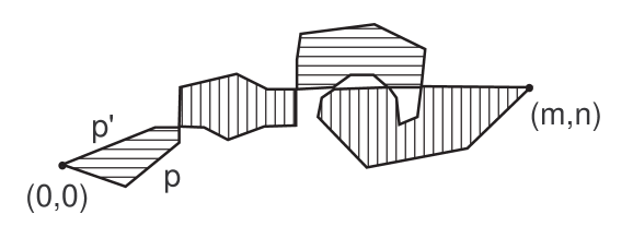
Figure 4: The $2$-chain $c(p,p^{\prime})$

We now define the signed area between $p$ and $p^{\prime}$ to be

$$S(p,p^{\prime})=\sum_{\alpha\in R}n_{\alpha}A(t_{\alpha}),$$ (36)

where $A(t_{\alpha})$ is the area of the triangle $t_{\alpha}$. This is clearly independent of the choice of triangulation of $\mathbb{R}^{2}$ compatible with $p,\,p^{\prime}$, since the sum of the areas of the triangles inside each enclosed region is the area of that region, whatever the triangulation.

We now have the main result of this section: for two paths $p,\,p^{\prime}$ as above the following relation holds:

$$U_{p}=q^{S(p,p^{\prime})}U_{p^{\prime}}.$$

This is proven as follows. Since $p$ and $p^{\prime}$ are homologous we can construct a sequence of paths between them by collapsing or adding one triangle at a time. Relation (34) for integer triangles generalizes to arbitrary triangles, and shows that the factor relating two successive paths in the sequence is $q^{n_{\alpha}t_{\alpha}}$, where $t_{\alpha}$ is the triangle by which the two successive paths differ. The overall factor, after cancellations, is determined by the chain $c(p,p^{\prime})$.

We note that the method of proof is reminiscent of Attal’s combinatorial approach to gerbes and the four-colour problem [11]. In principle an alternative approach would be to use the non-abelian Stokes theorem [12] and integrate the field strength

$$F=dA+\frac{1}{2}A\wedge A=[r_{1},r_{2}]\mathbb{I}dx\wedge dy$$

over the regions enclosed by $p$ and $p^{\prime}$. Although the field strength is non-vanishing, it commutes with the connection, which considerably simplifies the non-abelian Stokes formula.

3 $q$-deformed surface group representations

Classically there is a well-known correspondence between flat $G$-connections on a manifold $M$ and group homomorphisms from $\pi_{1}(M)$ to the gauge group $G$, up to equivalence (gauge equivalence for the connections and conjugation by a fixed element of $G$ for the group homomorphisms). Since here $M$ is a surface, such homomorphisms are known as surface group representations. Because of the constant connection gauge choice, the gauge equivalence for the connections is virtually trivialized, apart from the residual gauge freedom of equation (26), and the group $G$ is a diagonal subgroup of $SL(2,\mathbb{R})$.

Let $\Omega T^{2}$ denote the group of closed loops on $T^{2}$ identified with the PL paths $p$ from $(0,0)$ to an integer point in $\mathbb{R}^{2}$ introduced in the previous section. Then a surface group representation corresponds to an assignment $\phi$ to each $p\in\Omega T^{2}$ of an element $\phi(p)\in G$, such that

• $p_{1}\sim p_{2}\Longrightarrow\phi(p_{1})=\phi(p_{2})$ (where $\sim$ denotes “is homotopic to”)

• $\phi(p_{1}p_{2})=\phi(p_{1})\phi(p_{2})$.

Then a constant classical connection of the form $A=(r_{1}dx+r_{2}dy)\sigma_{3}$ gives rise to an assignment $\phi_{r_{1},r_{2}}$, namely

$$\phi_{r_{1},r_{2}}(p)=\exp\int_{p}A=\exp\left((mr_{1}+nr_{2})\sigma_{3}\right)$$

for any path $p$ connecting $(0,0)$ to $(m,n)$ (these are all homotopic).

Now we define a $q$-deformed version of the above appropriate to the constant quantum connections of Section 3. Let $\hat{G}$ denote the quantum matrices generated multiplicatively by matrices of the form (29)

$$\exp\left((ar_{1}+br_{2})\sigma_{3}\right)$$

where $a,b\in\mathbb{R}$. A $q$-deformed surface group representation is an assignment $\phi$ to each $p\in\Omega T^{2}$ of an element $\phi(p)\in\hat{G}$, such that

• $p_{1}\stackrel{{\scriptstyle c}}{{\sim}}p_{2}\Longrightarrow\phi(p_{1})=q^{S(p_{1},p_{2})}\phi(p_{2})$ where $\stackrel{{\scriptstyle c}}{{\sim}}$ denotes “is homotopic to, with the paths $p_{1},\,p_{2}$ in $\mathbb{R}^{2}$ differing by the $2$-chain $c$ of equation (35)”

• $\phi(p_{1}p_{2})=\phi(p_{1})\phi(p_{2})$.

This is well-defined. Firstly, if $p_{1}\stackrel{{\scriptstyle c}}{{\sim}}p_{2}$ and $p_{2}\stackrel{{\scriptstyle c^{\prime}}}{{\sim}}p_{3}$, we have

$$\left.\begin{array}[]{lcr}\phi(p_{1})&=&q^{S(p_{1},p_{2})}\phi(p_{2})\\ \phi(p_{2})&=&q^{S(p_{2},p_{3})}\phi(p_{3})\end{array}\right\}\Longrightarrow\phi(p_{1})=q^{S(p_{1},p_{2})+S(p_{2},p_{3})}\phi(p_{3})$$ (37)

but also

$$\phi(p_{1})=q^{S(p_{1},p_{3})}\phi(p_{3}).$$ (38)

Now since $\partial c=p_{1}-p_{3},\,\partial c^{\prime}=p_{2}-p_{3}$ and therefore $\partial(c+c^{\prime})=p_{1}-p_{3}$, it follows that $p_{1}\stackrel{{\scriptstyle c+c^{\prime}}}{{\sim}}p_{3}$ (see Figure 5).

Figure 5: Consistency of equations (37) and (38)

Then equations (37) and (38) are consistent since, writing $c=\sum_{\alpha\in R}n_{\alpha}t_{\alpha}$, $c^{\prime}=\sum_{\alpha\in R}n^{\prime}_{\alpha}t_{\alpha}$, and therefore $c+c^{\prime}=\sum_{\alpha\in R}(n_{\alpha}+n^{\prime}_{\alpha})t_{\alpha}$, we have, from (36),

$$S(p_{1},p_{3}) = \sum_{\alpha\in R}(n_{\alpha}+n^{\prime}_{\alpha})A(t_{\alpha})$$ (39)

$$= \sum_{\alpha\in R}n_{\alpha}A(t_{\alpha})+\sum_{\alpha\in R}n^{\prime}_{\alpha}A(t_{\alpha})$$

$$= S(p_{1},p_{2})+S(p_{2},p_{3}).$$

Secondly, let $p_{1}\stackrel{{\scriptstyle c}}{{\sim}}p_{3}$ and $p_{2}\stackrel{{\scriptstyle c^{\prime}}}{{\sim}}p_{4}$, i.e. $\partial c=p_{1}-p_{3}$, $\partial c^{\prime}=p_{2}-p_{4}$. Let $d$ be the $2$-chain obtained from $c^{\prime}$ by shifting the triangles by the vector $(m,n)$, the common endpoint of $p_{1}$ and $p_{3}$ (see Figure 6). Then

$$\partial(c+d)=p_{1}p_{2}-p_{3}p_{4}$$

Figure 6: Consistency of equations (40) and (41)

and

$$\phi(p_{1}p_{2}) = \phi(p_{1})\phi(p_{2})$$ (40)

$$= q^{S(p_{1},p_{3})}q^{S(p_{2},p_{4})}\phi(p_{3})\phi(p_{4})$$

$$= q^{S(p_{1},p_{3})+S(p_{2},p_{4})}\phi(p_{3}p_{4})$$

but also

$$\phi(p_{1}p_{2})=q^{S(p_{1}p_{2},p_{3}p_{4})}\phi(p_{3}p_{4}).$$ (41)

Equations (40) and (41) are consistent, since writing

$$c=\sum_{\alpha\in R}n_{\alpha}t_{\alpha}\quad c^{\prime}=\sum_{\alpha\in R}n^{\prime}_{\alpha}t_{\alpha}\quad d=\sum_{\alpha\in R}\tilde{n}^{\prime}_{\alpha}t_{\alpha}$$

it follows that

$$S(p_{1},p_{3})+S(p_{2},p_{4})=\sum_{\alpha\in R}(n_{\alpha}+{n}^{\prime}_{\alpha})A(t_{\alpha})$$

and

$$S(p_{1}p_{2},p_{3}p_{4}) = \sum_{\alpha\in R}(n_{\alpha}+\tilde{n}^{\prime}_{\alpha})A(t_{\alpha})$$

$$= \sum_{\alpha\in R}(n_{\alpha}+{n}^{\prime}_{\alpha})A(t_{\alpha})$$

$$= S(p_{1}p_{2},p_{3}p_{4}),$$

since the area is clearly unaffected by the translation.

By analogy with the classical case, a constant quantum connection

$$A=(r_{1}dx+r_{2}dy)\sigma_{3}$$

gives rise to a $q$-deformed surface group representation $\phi_{r_{1},r_{2}}$ by:

$$\phi_{r_{1},r_{2}}(p)=U_{p}$$

where $U_{p}$ was defined in (30). From the results of Section 3 (the multiplicativity of the assignment $p\mapsto U_{p}$, and the area phases relating the matrices for homotopic paths) it is clear that $\phi_{r_{1},r_{2}}$ satisfies the conditions for being a $q$-deformed surface group representation.

4 The Modular Group

Consider the piecewise linear (PL) paths of Section 2. Since $SL(2,\mathbb{Z})$ acts on $\mathbb{R}^{2}$ by multiplication, fixes the origin and preserves the lattice of points $\mathbb{Z}^{2}\in\mathbb{R}^{2}$, it maps straight segments to straight segments and PL paths to PL paths. This defines an action of $SL(2,\mathbb{Z})$ on the collection of matrices $U_{p}$ of equation (30) by

$$M.U_{p}=U_{M.p}.$$ (42)

For straight paths $(m,n)$ - for example those appearing in equation (31) - we can make contact with earlier work [3, 4] by setting $U_{1}=U_{(1,0)}$, $U_{2}=U_{(0,1)}$ and checking the action of the standard generators of $SL(2,\mathbb{Z})$

$$T=\left(\begin{array}[]{clcr}1&0\\ 1&1\end{array}\right),\qquad S=\left(\begin{array}[]{clcr}0&-1\\ 1&0\end{array}\right)$$ (43)

on $U_{1}$ and $U_{2}$, namely

$$T.U_{1} = T.U_{(1,0)}=U_{(1,1)}=q^{-1/2}U_{1}U_{2}$$

$$T.U_{2} = T.U_{(0,1)}=U_{(0,1)}=U_{2}$$

$$S.U_{1} = S.U_{(1,0)}=U_{(0,1)}=U_{2}$$

$$S.U_{2} = S.U_{(0,1)}=U_{(-1,0)}=U_{1}^{-1}$$ (44)

which preserve the fundamental relation (14). In the first of (44) (the equation for $T.U_{1}$) the triangle relation (34) was used. The first two of (44) correspond to the more familiar classical transformations

$$U_{1}\stackrel{{\scriptstyle T}}{{\to}}U_{1}U_{2},\qquad U_{2}\stackrel{{\scriptstyle T}}{{\to}}U_{2},$$ (45)

whereas the last two correspond to

$$U_{1}\stackrel{{\scriptstyle S}}{{\to}}U_{2},\qquad U_{2}\stackrel{{\scriptstyle T}}{{\to}}U_{1}^{-1},$$ (46)

which differ from (44) by a phase, but still preserve (14). Note that in both cases $S^{2}=-\mathbb{I},S^{4}=\mathbb{I},(ST)^{3}=\mathbb{I}$, both algebraically and geometrically. For example, algebraically $T.U_{1}^{-1}=q^{1/2}U_{2}^{-1}U_{1}^{-1}$ whereas geometrically $T.U_{1}^{-1}=T.U_{(-1,0)}=U_{(-1,-1)}$. These are equal when the triangle relation (34) is applied.

We can also define a dual action of $SL(2,\mathbb{Z})$ on the $q$-deformed surface group representations of Section 3 for generic paths $p$ by

$$(M.\phi)(p)=\phi(M^{-1}.p).$$ (47)

This is a left action in the usual way since

$$(M_{1}.(M_{2}.\phi))(p) = (M_{2}.\phi)(M_{1}^{-1}.p)$$ (48)

$$= \phi(M_{2}^{-1}.(M_{1}^{-1}.p))$$

$$= \phi(M_{2}^{-1}M_{1}^{-1}).p))$$

$$= \phi((M_{1}M_{2})^{-1}.p))$$

$$= (M_{1}M_{2}.\phi)(p).$$

It is also well defined since, for $p_{1}\stackrel{{\scriptstyle c}}{{\sim}}p_{2}$,

$$(M.\phi)(p_{1}) = \phi(M^{-1}.p_{1})$$ (49)

$$= q^{S(M^{-1}.p_{1},M^{-1}.p_{2})}\phi(M^{-1}.p_{2})$$

$$= q^{S(p_{1},p_{2})}(M.\phi)(p_{2})$$

since $M\in SL(2,\mathbb{Z})$ has determinant $1$ and thus preserves areas. Moreover,

$$(M.\phi)(p_{1}p_{2}) = \phi(M^{-1}.(p_{1}p_{2}))$$ (50)

$$= \phi((M^{-1}.p_{1})(M^{-1}.p_{2}))$$

$$= \phi(M^{-1}.p_{1})\phi(M^{-1}.p_{2})$$

$$= (M.\phi)(p_{1})(M.\phi)(p_{2}).$$

5 The Goldman bracket

There is a classical bracket due to Goldman [10] for functions $T(\gamma)={\rm tr}\,U_{\gamma}$ defined on homotopy classes of loops $\gamma$, which for $U_{\gamma}\in SL(2,\mathbb{R})$ is (see [10] Thm. 3.14, 3.15 and Remark (2), p. 284):

$$\{T(\gamma_{1}),T(\gamma_{2})\}=\sum_{S\in\gamma_{1}\sharp\gamma_{2}}\epsilon(\gamma_{1},\gamma_{2},S)(T(\gamma_{1}S\gamma_{2})-T(\gamma_{1}S\gamma_{2}^{-1})).$$ (51)

Here $\gamma_{1}\sharp\gamma_{2}$ denotes the set of (transversal) intersection points of $\gamma_{1}$ and $\gamma_{2}$ and $\epsilon(\gamma_{1},\gamma_{2},S)$ is the intersection index for the intersection point $S$. $\gamma_{1}S\gamma_{2}$ and $\gamma_{1}S\gamma_{2}^{-1}$ denote loops which are rerouted at the intersection point $S$. In the following we explain and use these concepts, and show how formula (51) appears in the context of the PL paths introduced in Section 2. Equation (51) may be quantized in two different but equivalent forms using the concept of area phases for homotopic paths which was developed in Sections 2 and 3.

5.1 The Fundamental Reduction

In order to study intersections of “straight” loops, represented in $\mathbb{R}^{2}$ by straight paths between $(0,0)$ and integer points $(m,n)$, it is useful to consider their reduction to a fundamental domain of $\mathbb{R}^{2}$, namely the square with vertices $(0,0),(1,0),(1,1),(0,1)$.

We give some examples of fundamental reduction. Figure 7 shows a path in the first quadrant, namely the path $(2,1)$, and its reduction to the fundamental domain

Figure 7: The path $(2,1)$ and its fundamental reduction

whereas in other quadrants fundamentally reduced paths start at other vertices (not $(0,0)$). For example in the second quadrant the path $(-1,2)$ will (in the fundamental domain) start at $(1,0)$ and end at $(0,1)$, as shown in Figure 8.

Figure 8: The path $(-1,2)$ and its fundamental reduction

Examples of the reduction of paths from the third quadrant (the path $(-1,-1)$, starting at $(1,1)$ and ending at $(0,0)$) and the fourth quadrant (the path $(2,-1)$, starting at $(0,1)$ and ending at $(1,0)$) are shown in Figures 9 and 10 respectively.

Figure 9: The path $(-1,-1)$ and its fundamental reduction

Figure 10: The path $(2,-1)$ and its fundamental reduction

When the path $(m,n)$ is a multiple of another integer path, we say it is reducible. Otherwise it is irreducible. Figure 11 shows how this multiplicity is indicated in the fundamental reduction.

Figure 11: The path $(-2,4)$ and its fundamental reduction

5.2 Intersections

It is clear from Section 5.1 that two paths intersect at any points where their fundamental reductions intersect. We may only consider transversal intersections, namely when their respective tangent vectors are not collinear. For paths of multiplicity $1$ intersecting at a point, we say that their intersection number at that point is $+1$ if the angle from the first tangent vector to the second is between $0$ and $180$ degrees, and $-1$ if between $180$ and $360$ degrees. For paths of multiplicity greater than $1$, the intersection number is multiplied by the multiplicities of the paths involved. We denote the intersection number between two paths $p_{1}$ and $p_{2}$ at a point $P$ (or $P,Q,R$ if more than one) by $\epsilon(p_{1},p_{2},P)$. The total intersection number for two paths is the sum of the intersection numbers for all the intersection points, denoted $\epsilon(p_{1},p_{2})$. We list some simple (and not so simple) examples (in the fundamental domain) of single and multiple intersections.

1. If $p_{1}=(1,0)$ and $p_{2}=(0,1)$ then there is a single intersection at the point $(0,0)$ with $\epsilon=+1$.

2. If $p_{1}=(2,1)$ and $p_{2}=(0,1)$ then there are two intersections, one at the point $P=(0,0)$, and one at the point $Q=(0,\frac{1}{2})$, each with $\epsilon=+1$, so the total intersection number is $\epsilon=+2$

3. If $p_{1}=(1,2)$ and $p_{2}=(2,1)$ then there are three intersections, one at the point $P=(0,0)$, and two others at the points $Q=(\frac{2}{3},\frac{1}{3})$ and $R(\frac{1}{3},\frac{2}{3})$ (see figure), each with $\epsilon=-1$, so the total intersection number is $\epsilon=-3$ (the point $S=(1,1)$ does not contribute since it coincides with the point $P$)

4. If $p_{1}=(1,1)$ and $p_{2}=(-1,2)$ then there are three intersections, one at the point $P=(0,0)$, and two others at the points $Q=(\frac{2}{3},\frac{2}{3})$ and $R=(\frac{1}{3},\frac{1}{3})$ (see figure), each with $\epsilon=+1$, so the total intersection number is $\epsilon=+3$

We remark that

1. all intersections between a given pair of straight paths have the same sign, since in this representation their tangent vectors have constant direction along the loops.

2. the total intersection number between $p_{1}=(m,n)$ and $p_{2}=(s,t)$ is given by the determinant

   $$\epsilon(p_{1},p_{2})=\left|\begin{array}[]{clcr}m&n\\ s&t\end{array}\right|=mt-ns$$ (52)

   This is shown by using the fact that the total intersection number is invariant under deformation, i.e. homotopy

   $$\epsilon((m,n),(s,t)) = \epsilon((m,0)+(0,n),(s,0)+(0,t))$$ (53)

   $$= \epsilon((m,0),(0,t))+\epsilon((0,n),(s,0))$$

   $$= mt-ns.$$

   Relation (52) is easily checked for the above examples.

5.3 Reroutings

Consider two straight paths $p_{1}$ and $p_{2}$ and let $P$ be a point at which they intersect. The positive and negative reroutings are the paths denoted by $p_{1}Pp_{2}$ and $p_{1}Pp_{2}^{-1}$ respectively, where $p_{2}^{-1}=(-s,-t)$ if $p_{2}=(s,t)$. These reroutings are defined as follows: starting at the basepoint follow $p_{1}$ to $P$, continue on $p_{2}$ (or $p_{2}^{-1}$) back to $P$, then finish along $p_{1}$. Note that, in accordance with the above rule, if the intersection point $P$ is the basepoint itself, the reroutings $p_{1}Pp_{2}$ and $p_{1}Pp_{2}^{-1}$ start by following $p_{2}$ (or $p_{2}^{-1}$) from the basepoint back to the basepoint, and then follow $p_{1}$ from the basepoint back to the basepoint. Here we show the reroutings ($p_{1}Pp_{2}$ and $p_{1}Pp_{2}^{-1}$ respectively, and at the various intersection points $P,Q,R$ if more than one) for the four examples of Section 5.2, using the non–reduced paths which are more convenient here.

1. $P=(0,0),p_{1}=(1,0),p_{2}=(0,1)$      

2. (a) $P=(0,0),p_{1}=(2,1),p_{2}=(0,1)$       (b) $Q=(0,\frac{1}{2}),p_{1}=(2,1),p_{2}=(0,1)$      

3. (a) $P=(0,0),p_{1}=(1,2),p_{2}=(2,1)$       (b) $Q=(\frac{2}{3},\frac{1}{3}),p_{1}=(1,2),p_{2}=(2,1)$       (c) $R=(\frac{1}{3},\frac{2}{3}),p_{1}=(1,2),p_{2}=(2,1)$      

4. (a) $P=(0,0),p_{1}=(1,1),p_{2}=(-1,2)$       (b) $Q=(\frac{2}{3},\frac{2}{3}),p_{1}=(1,1),p_{2}=(-1,2)$       (c) $R=(\frac{1}{3},\frac{1}{3}),p_{1}=(1,1),p_{2}=(-1,2)$      

In each of the above examples, and for each intersection point $P,Q,R$, it is clear that $p_{1}Pp_{2}\sim(m+s,n+t)$ and $p_{1}Pp_{2}^{-1}\sim(m-s,n-t)$.

5.4 The Goldman bracket

We can assign classical functions to the straight paths $(m,n)$ of Section 5.1 as follows

$$T(m,n)=e^{mr_{1}+nr_{2}}+e^{-mr_{1}-nr_{2}},$$ (54)

i.e. $T(m,n)={\rm tr}~{}~{}U_{(m,n)}$ where $U_{(m,n)}$ is of the form (33) with $r_{1},\,r_{2}$ classical parameters. In terms of the Poisson bracket (5) the Poisson bracket between these functions for two paths $(m,n)$ and $(s,t)$ is

$$\{T(m,n),T(s,t)\}=(mt-ns)(T(m+s,n+t)-T(m-s,n-t))\{r_{1},r_{2}\}$$ (55)

Equation (55) may be regarded as a particular case of the Goldman bracket (51) (modulo rescaling $\{r_{1},r_{2}\}$ to $1$), since $(m,n)$ and $(s,t)$ have total intersection index $mt-ns$, and the rerouted paths $p_{1}Qp_{2}$ and $p_{1}Qp_{2}^{-1}$, where $p_{1}=(m,n)$ and $p_{2}=(s,t)$, are all homotopic to $(m+s,n+t)$ and $(m-s,n-t)$ respectively.

The bracket (55) can be quantized using the triangle identity (see (34))

$$e^{mr_{1}+nr_{2}}e^{sr_{1}+tr_{2}}=q^{(mt-ns)/2}e^{(m+s)r_{1}+(n+t)r_{2}}$$ (56)

and the result is the commutator

$$[T(m,n),T(s,t)]=(q^{\frac{(mt-ns)}{2}}-q^{-\frac{(mt-ns)}{2}})(T(m+s,n+t)-T(m-s,n-t)).$$ (57)

The antisymmetry of (57) is evident (from (54) $T(m,n)=T(-m,-n)$). It can be checked that (57) satisfies the Jacobi identity, and that the classical limit $q\to 1,\hbar\to 0$

$$\{,\}=lim_{\hbar\to 0}\frac{[,]}{i\hbar}$$

of (57) is precisely (55).

We will now give a different version of equation (57) which treats each intersection point individually, and uses rerouted paths homotopic to “straight line” paths as discussed in Section 5.3, since we have already seen in Section 2 that homotopic paths no longer have the same quantum matrix assigned to them, but only the same matrix up to a phase. Thus for an arbitrary PL path $p$ from $(0,0)$ to $(m,n)$, set

$$T(p)=q^{S(p,(m,n))}T(m,n).$$ (58)

The factor appearing in (58) is the same as that relating the quantum matrices $U_{p}$ and $U_{(m,n)}$, where $(m,n)$ is the straight path.

Firstly we will show how to rewrite (57) in terms of the rerouted paths of Section 5.3 for one of the previous examples (example 3 of Section 5.2). In this example $p_{1}=(1,2),\,p_{2}=(2,1)$, and we have, from (57)

$$[T(1,2),T(2,1)]=(q^{-3/2}-q^{3/2})(T(3,3)-T(-1,1)).$$ (59)

The intersections occur at the points $P,R,Q$ (in that order, counting along $p_{1}$) as shown in Figure 12. For the positively rerouted paths at these points we have the following equations

$$T((1,2)P(2,1)) = T((2,1)(1,2))=q^{3/2}T(3,3)$$ (60)

$$T((1,2)R(2,1)) = q^{-1}T((1,2)P(2,1))$$ (61)

$$T((1,2)Q(2,1)) = q^{-1}T((1,2)R(2,1))$$ (62)

and for the negative reroutings

$$T((1,2)P(-2,-1)) = T((-2,-1)(1,2))=q^{-3/2}T(-1,1)$$ (63)

$$T((1,2)R(-2,-1)) = qT((1,2)P(-2,-1))$$ (64)

$$T((1,2)Q(-2,-1)) = qT((1,2)R(-2,-1)).$$ (65)

The factors appearing in equations (61), (62), (64) and (65) (the reroutings at the points $R$ and $Q$) are shown in Figure 12, where it is clear that each large parallelogram is divided into three equal parallelograms, each of unit area. The factors in (60) and (63) (the reroutings at the point $P$) come from the triangle equation (34), and are shown in Figure 13, where the triangles have signed area $+\frac{3}{2}$ and $-\frac{3}{2}$ respectively.

Figure 12: The reroutings $(1,2)S(2,1)$ and $(1,2)S(-2,-1)$ for $S=P,R,Q$

Figure 13: Factors for the reroutings $(1,2)P(2,1)$ and $(1,2)P(-2,-1)$

After a simple calculation we find that equation (59) can be rewritten in the form:

$$[T(1,2),T(2,1)]=\sum_{S=P,R,Q}(q^{-1}-1)T((1,2)S(2,1))+(q-1)T((1,2)S(-2,-1)).$$ (66)

In the general case, for $p_{1}=(m,n)$ and $p_{2}=(s,t)$ with $mt-ns\neq 0$, we postulate that

$$[T(p_{1}),T(p_{2})]=\sum_{Q\in p_{1}\sharp p_{2}}(q^{\epsilon(p_{1},p_{2},Q)}-1)T(p_{1}Qp_{2})+(q^{-\epsilon(p_{1},p_{2},Q)}-1)T(p_{1}Qp_{2}^{-1})$$ (67)

quantizes the Goldman bracket (51).

To prove equation (67) we first assume that both $p_{1}$ and $p_{2}$ are irreducible, i.e. not multiples of other integer paths, and study the reroutings $p_{1}Qp_{2}$ with $Q$ an intersection point, as discussed in Section 5.3. They are paths similar to those of Figure 12, namely following $p_{1}$ to $Q$, then rerouting along a path parallel to $p_{2}$, then finishing along a path parallel to $p_{1}$. The reroutings along $p_{2}$ obviously must pass through an integer point inside the parallelogram formed by $p_{1}$ and $p_{2}$ (apart from when the intersection point is the origin). They also clearly pass through only one integer point since $p_{2}$ is irreducible. Consider two adjacent lines inside the parallelogram parallel to $p_{2}$ and passing through integer points. We claim that the area of each parallelogram between them is $1$. Consider for instance one of the middle parallelograms in Figure 12 (whose area we saw previously was $1$ as the three parallelograms are clearly of equal area and the area of the large parallelogram is $3$). This is the same area as that of a parallelogram with vertices at integer points, as can be shown, for example, by cutting it into two pieces along the line between (1,1) and (2,2), then regluing them together into a parallelogram with vertices at (1,1), (2,2), (3,2) and (4,3), as indicated in Figure 14. This latter area is equal to $1$ from Pick’s theorem [13] which states that the area $A(P)$ of a lattice polygon $P$ is

$$A(P)=I(P)+B(P)/2-1,$$ (68)

where $I(P)$ is the number of interior lattice points and $B(P)$ is the number of boundary points (for the parallelogram in the example $I(P)=0$ since the lines parallel to $p_{2}$ are adjacent, and $B(P)=4$ from the integer points at the four vertices, so $A(P)=0+4/2-1=1$.) Therefore in general the parallelogram determined by $p_{1}$ and $p_{2}$, whose total area is $A=|mt-ns|$, is divided up into $A$ smaller parallelograms of equal area by lines parallel to $p_{2}$ passing through the interior integer points of the parallelogram. The fact that the total area is equal to the number of internal integer points $+1$ is again a consequence of Pick’s theorem.

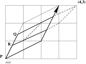
Figure 14: The area of the middle parallelogram is $1$

We can now calculate the first term (the positive reroutings shown for the example in Figure 12) in the sum on the r.h.s. of (67), using equation (58), and show that it is equal to the first term on the r.h.s. of (57). Consider first the case $\epsilon(p_{1},p_{2},Q)=-1$. The rerouting at the origin satisfies, using the triangle equation (34),

$$T(p_{1}\,(0,0)\,p_{2})=q^{A/2}T(m+s,n+t),$$

where the area of the parallelogram determined by $p_{1},\,p_{2}$ is $A=-(mt-ns)$. The next rerouted path adjacent to $p_{1}\,(0,0)\,p_{2}$, rerouted at $Q_{1}$ say (in the example $Q_{1}=R$) satisfies

$$T(p_{1}\,Q_{1}\,p_{2})=q^{-1}T(p_{1}\,(0,0)\,p_{2})$$

since we have shown that the signed area between the paths is $-1$. Similarly each successive adjacent path rerouted at $Q_{2},Q_{3},\dots$ satisfies

$$T(p_{1}\,Q_{i}\,p_{2})=q^{-1}T(p_{1}\,Q_{i-1}\,p_{2}).$$ (69)

with $Q_{0}$ the origin $(0,0)$. It follows that

$$\sum_{Q\in p_{1}\sharp p_{2}}(q^{-1}-1)T(p_{1}Qp_{2})$$ (70)

$$= (q^{-1}-1)q^{A/2}(1+q^{-1}+\dots+q^{-(A-1)})T(m+s,n+t)$$

$$= (q^{-1}-1)q^{A/2}\frac{1-q^{-A}}{1-q^{-1}}T(m+s,n+t)$$

$$= (q^{-A/2}-q^{A/2})T(m+s,n+t)$$

$$= (q^{(mt-ns)/2}-q^{-(mt-ns)/2})T(m+s,n+t).$$

When $\epsilon(p_{1},p_{2},Q)=+1$ the calculation is identical to (70) but with $q$ rather than $q^{-1}$, and with the area of the triangle now equal to $A/2$, where $A=mt-ns$, namely

$$\sum_{Q\in p_{1}\sharp p_{2}}(q-1)T(p_{1}\,Q\,p_{2})$$ (71)

$$= (q-1)q^{-A/2}(1+q^{1}+\dots+q^{A-1})T(m+s,n+t)$$

$$= (q^{A/2}-q^{-A/2})T(m+s,n+t)$$

$$= (q^{(mt-ns)/2}-q^{-(mt-ns)/2})T(m+s,n+t).$$

Diagrammatically this corresponds to dividing up the first parallelogram in Figure 12 by lines passing through the integer points in the interior, but parallel to $(1,2)$, as opposed to $(2,1)$.

In an entirely analogous way the second terms (the negative reroutings) on the r.h.s. of (57) and (67) can be shown to be equal - the second figure of Figure 12 can be used as a guide.

When $p_{1}$ is reducible, i.e. $p_{1}=c(m^{\prime},n^{\prime}),\,c\in\mathbb{N},m^{\prime},n^{\prime}\in\mathbb{Z}$, and $p_{2}$ is irreducible, formula (67) applies exactly as for the irreducible case, since there are $c$ times as many rerouted paths compared to the case when $p_{1}=(m^{\prime},n^{\prime})$. An example is $p_{1}=(2,0),\,p_{2}=(1,2)$, where the first term on the r.h.s. of (57) is equal to the first term on the r.h.s. of (67):

$$(q^{2}-q^{-2})T(3,2) = (q-1)q^{-2}(1+q+q^{2}+q^{3})T(3,2)$$ (72)

$$= \sum_{Q\in p_{1}\sharp p_{2}}(q-1)T(p_{1}Qp_{2}).$$

There are four rerouted paths in the final summation rerouting at $(0,0)$, $(1/2,0)$, $(1,0)$ and $(3/2,0)$ along $p_{1}$.

If $p_{2}$ is reducible we must use multiple intersection numbers in (67), i.e. not simply $\pm 1$. Suppose $p_{1}=(m,n)$ and $p_{2}=(s,t)=c(s^{\prime},t^{\prime})$, $c\in\mathbb{N},s^{\prime},t^{\prime}\in\mathbb{Z}$. Then for example the first term on the r.h.s. of (67) with $mt-ns>0$ is

$$(q^{(mt-ns)/2})-q^{-(mt-ns)/2})T(m+s,n+t)$$ (73)

$$= (q^{c(mt^{\prime}-ns^{\prime})}-1)q^{-(mt-ns)/2}T(m+s,n+t)$$

$$= (q^{c}-1)q^{-(mt-ns)/2}(1+q^{c}+\dots+q^{c(mt^{\prime}-ns^{\prime}-1)})T(m+s,n+t)$$

$$= \sum_{Q\in p_{1}\sharp p_{2}}(q^{c}-1)T(p_{1}Qp_{2}).$$

The factor $(q^{c}-1)$ is the quantum multiple intersection number at the $mt^{\prime}-ns^{\prime}$ intersection points. The calculation can be regarded as doing equation (71) backwards and substituting $q$ by $q^{c}$ and $mt-ns$ by $mt^{\prime}-ns^{\prime}$. An example is given by $p_{1}=(2,1),\,p_{2}=(0,2)$, for which double intersections occur along $p_{1}$ at the origin and at $(1,1/2)$. From (73) the first term on the r.h.s. of (67) is

$$(q^{2}-q^{-2})T(2,3) = (q^{2}-1)q^{-2}(1+q^{2})T(2,3)$$ (74)

$$= (q^{2}-1)(T(p_{1}\,(0,0)\,Qp_{2})+T(p_{1}\,(1,1/2)\,p_{2}).$$

6 Conclusions

The quantum geometry emerging from the use of a constant quantum connection exhibits some surprising features. The phase factor appearing in the fundamental relation (31) acquires a geometrical origin as the signed area phase relating two integer PL paths, corresponding to two different loops on the torus e.g. as in Figure 2. The signed area phases between PL paths have good properties, and lead to a natural concept of $q$-deformed surface group representations. The classical correspondence between flat connections (local geometry) and holonomies, i.e. group homomorphisms from $\pi_{1}$ to $G$ (non-local geometry) thus has a natural quantum counterpart. It is interesting to speculate that the signed area phases could be related to gerbe parallel transport [14].

The signed area phases also appear in a quantum version (67) of a classical bracket (51) due to Goldman [10], where classical intersection numbers $\pm\epsilon(p_{1},p_{2},Q)$ are replaced by quantum single and multiple intersection numbers $(q^{\pm\epsilon(p_{1},p_{2},Q)}-1)$.

The quantum bracket for homotopy classes represented by straight lines (57) is easily checked since all the reroutings are homotopic. However the r.h.s. of the bracket (67) is expressed in terms of rerouted paths using the signed area phases and a far subtler picture emerges.

The quantum bracket for straight lines (57) is manifestly antisymmetric. Although we have shown that (57) and (67) are equivalent the antisymmetry of (67) is not at all obvious. This antisymmetry can be checked however when both paths are irreducible e.g. the example in Section 5.4, even though the intersections in the two cases may occur in a different order. When one of the paths is reducible then the r.h.s. is expressed in terms of either multiple reroutings with single intersection numbers (for $p_{1}$ reducible) or single reroutings with multiple intersection numbers (for $p_{2}$ reducible). The case when both $p_{1}$ and $p_{2}$ are reducible is a combination of the above. There should be an interplay between the two scenarios.

It is not difficult to show that the Jacobi identity holds for the quantum bracket for straight paths (57) since the r.h.s. may also be expressed in terms of straight paths, with suitable phases. It must also hold for (67) since they are equivalent. To show this explicitly for arbitrary PL paths implies extending the bracket (67) to arbitrary PL paths, without identifying homotopic paths. It should also be possible to treat higher genus surfaces (of genus $g$) in a similar fashion by introducing the same constant quantum connection on a domain in the $xy$ plane bounded by a $4g$–gon with the edges suitably identified [15]. One could then define holonomies of PL loops on this domain and study their behaviour under intersections, in an analogous fashion to the genus $1$ case studied here. These, and related questions, will be studied elsewhere.

References

- [1] J.E. Nelson, T. Regge and F. Zertuche, Homotopy Groups and dimensional Quantum De Sitter Gravity, Nucl. Phys. B339 (1990) 516–532.
- [2] J.E. Nelson and T. Regge, Quantum Gravity, Phys. Lett. B272 (1991) 213–216.
- [3] J.E. Nelson and R.F. Picken, Quantum holonomies in - dimensional gravity, Phys. Lett. B471 (2000) 367–372.
- [4] J.E. Nelson and R.F. Picken, Quantum matrix pairs, Lett. Math. Phys. 52 (2000) 277–290.
- [5] S. Carlip, Quantum gravity in dimensions, Cambridge Monographs on Mathematical Physics, Cambridge University Press, Cambridge (1998).
- [6] S. Carlip S. and J.E. Nelson, Comparative Quantizations of 2+1 Gravity, Phys. Rev. D51, 10 (1995) 5643–5653. Equivalent Quantisations of 2+1 Gravity, Phys. Lett. B324 (1994) 299–302.
- [7] J.E. Nelson and R.F. Picken, Parametrization of the moduli space of flat connections on the torus, Lett. Math. Phys. 59 (2002) 215–226.
- [8] J.E. Nelson and V. Moncrief, Constants of the motion and the conformal anti-de Sitter algebra in (2+1)-Dimensional Gravity, Int. J. Mod. Phys. D6, 5 (1997) 545–562.
- [9] A. Mikovic and R.F. Picken, Super Chern-Simons theory and flat super connections on a torus, Adv. Theor. Math. Phys. 5 (2001) 243–263.
- [10] W.M. Goldman, Invariant functions on Lie groups and Hamiltonian flows of surface group representations, Invent. Math. 85 (1986) 263–302.
- [11] R. Attal, Combinatorics of non-Abelian Gerbes with Connection and Curvature, math-ph/0203056, to appear in Annales Fond. Louis Broglie.
- [12] B. Broda, Non-Abelian Stokes Theorem in Action, in “Modern Nonlinear Optics”, Part 2, ed. M. W. Evans, Wiley, pp. 429–468, (2001).
- [13] G. Pick, Geometrisches zur Zahlentheorie, Sitzenber. Lotos (Prague) 19 (1899) 311–319 and e.g. H.S.M. Coxeter, Introduction to Geometry, 2nd ed. New York: Wiley, p. 209 (1969).
- [14] M. Mackaay and R. Picken, Holonomy and Parallel Transport for Abelian Gerbes, Adv. Math. 170 (2002) 287–339, and R. Picken, TQFT and gerbes, Alg. Geom. Topology 4 (2004) 243-272.
- [15] D. Hilbert and S. Cohn-Vossen, Geometry and the Imagination, (transl. Nemenyi, P.) Chelsea Publishing Company, New York, (1990).