Linear stability analysis of hedgehogs in the Skyrme model on the three-sphere.
Critical phenomena and spontaneously broken reflection symmetry.

Abstract

This paper is devoted to the linear stability analysis of the whole spectrum of static hedgehog solutions of the Skyrme model on the three-sphere of radius $L$. These solutions are described by profiles $F(\psi)$ that satisfy the equation

$$\left(L+\frac{2}{L}\frac{\sin^{2}{F(\psi)}}{\sin^{2}{\psi}}\right)\sin^{2}{\psi}F^{\prime\prime}(\psi)+\left(L+\frac{1}{L}\frac{\sin{2F(\psi)}}{\sin{2\psi}}F^{\prime}(\psi)\right)\sin{2\psi}F^{\prime}(\psi)$$

$$-\left(L+\frac{1}{L}\frac{\sin^{2}{F(\psi)}}{\sin^{2}{\psi}}\right)\sin{2F(\psi)}=0,$$

where $\psi\in[0,\pi]$, $F(0)=0$, $F(\pi)=\mathcal{Q}\pi$ and $\mathcal{Q}$ is an integer which has the interpretation of topological charge. This work is the continuation of the paper [3] where these solutions were classified. It turns out that only solutions that in the limit $L\to\infty$ tend to skyrmions (localized at the poles) are linearly stable. The other solutions are unstable and, for a given solution, the number of instabilities, for $L$ sufficiently large, is equal to the index of a harmonic map to which this solution tends pointwise in the limit $L\to\infty$. Such solutions, which in addition have a definite parity, undergo a transition by $+1$ in the number of instabilities as $L$ grows. Due to the instability, new solutions, with spontaneously broken reflection symmetry, are born by bifurcations. In the case of the $1$-skyrmion this critical phenomenon can be fully described analytically. This allows of prediction the unique series expansions for the profile of the $1$-skyrmion and for its energy, though their expansion coefficients are not given in a general form, and read respectively

$$F(\psi) = \psi+x\sin{\psi}+x^{2}\frac{3}{20}\sin{2\psi}-x^{3}\left(\frac{29369}{316800}\sin{\psi}-\frac{11}{480}\sin{3\psi}\right)+\mathcal{O}{(x^{4})}$$

$$\frac{E[F]}{12\pi^{2}} = \frac{3\sqrt{2}}{4}\left(1+\frac{11}{180}x^{2}-\frac{209}{10800}x^{4}+\frac{5209}{864000}x^{6}+\mathcal{O}{(x^{6})}\right),\qquad x=\pm\sqrt{\frac{60}{11}\left(\frac{L}{\sqrt{2}}-1\right)}.$$

The above expansions are valid in some right neighbourhood of the critical radius $L=\sqrt{2}$ at which the $1$-skyrmion (with broken reflection symmetry) is born by a ’costing no energy’ excitation of the marginal stability mode of parity $+1$ on the identity solution, which has parity $-1$. To the author’s best knowledge the series were not given in literature so far. A similar mechanism of spontaneous breaking of parity is also observed when other solutions appear by bifurcations from symmetric solutions.

1 The Skyrme model on $\mathcal{S}^{3}$

The Skyrme model is defined by the action which written in generally covariant form reads

$$\mathcal{S}[U]=\int\sqrt{-g}\mathrm{d}^{4}x\left(\frac{1}{4}\mathbf{f}_{\pi}^{2}\mathrm{Tr}\left(K_{\mu}K^{\mu}\right)+\frac{1}{32\mathbf{e}^{2}}\mathrm{Tr}\left([K_{\mu},K_{\nu}][K^{\mu},K^{\nu}]\right)\right),$$ (1.1)

where $U$ is the basic chiral $SU(2)$-valued scalar field and $K_{\mu}=\mathrm{i}U^{+}\partial_{\mu}U$ is a Lie algebra valued four-current. We use the convention $(+,-,-,-)$ for the signature of the canonical quadratic form associated with a metric tensor. The first integrand is the $\sigma$-term, the second one was introduced by Skyrme in [9] to ensure the existence of solitons, but its shape may be also determined by using geometrical arguments [7],[5]. Both these terms have mutually inverse scale dependence, thus compete against each other. Unlike in the Skyrme model on flat space, in addition to the natural size of a soliton $(\mathbf{e}\mathbf{f}_{\pi})^{-1}$, we have another natural size at our disposal which is introduced by the radius $R$ of the base three-sphere. Their quotient $L=\mathbf{e}\mathbf{f}_{\pi}R$ (which is a dimensionless number as the $\pi$) must have nontrivial consequences to our model since the parameter $L$, as a remnant of the mentioned competition, enters the equations of motion.

In [3] we found and classified all static, finite energy, spherically symmetric and equivariant mappings $F$ from the base space – the three-sphere of radius $R$, to the target space – the group $SU(2)$. These mappings are regular solutions of the equation

$$\left(L+\frac{2}{L}\frac{\sin^{2}{F(\psi)}}{\sin^{2}{\psi}}\right)\sin^{2}{\psi}F^{\prime\prime}(\psi)+$$

$$\left(L+\frac{1}{L}\frac{\sin{2F(\psi)}}{\sin{2\psi}}F^{\prime}(\psi)\right)\sin{2\psi}F^{\prime}(\psi)-$$

$$\left(L+\frac{1}{L}\frac{\sin^{2}{F(\psi)}}{\sin^{2}{\psi}}\right)\sin{2F(\psi)}=0,$$ (1.2)

which is singular on boundaries. We utilized the canonical correspondence between points $(\Psi,\Theta,\Phi)$ on $\mathcal{S}^{3}$ and elements of $SU(2)$ (the last is metrically equivalent to $\mathcal{S}^{3}$), that is if $U\in SU(2)$ then

$$U(\Psi,\Theta,\Phi)=\left(\begin{array}[]{cc}\cos{\Psi}+\mathrm{i}\sin{\Psi}\cos{\Theta}&\mathrm{i}\sin{\Psi}\sin{\Theta}e^{-\mathrm{i}\Phi}\\ \mathrm{i}\sin{\Psi}\sin{\Theta}e^{\mathrm{i}\Phi}&\cos{\Psi}-\mathrm{i}\sin{\Psi}\cos{\Theta}\end{array}\right).$$

The base three sphere is endowed with the standard spherical coordinates $(\psi,\vartheta,\varphi)$ in which the line element reads

$$\mathrm{d}{s}^{2}=R^{2}\left({\mathrm{d}{\psi}^{2}+\sin^{2}{\psi}\left({\mathrm{d}{\vartheta}^{2}+\sin^{2}{\vartheta}\mathrm{d}{\varphi}^{2}}\right)}\right),\quad\{\psi,\vartheta,\varphi\}\in[0,\pi]\times[0,\pi]\times[0,2\pi].$$

The equivariance of the mapping $\mathcal{S}^{3}\to\mathcal{S}^{3}$ means that

$$F:\quad\mathcal{S}^{3}\ni(\psi,\vartheta,\varphi)\rightarrow(\Psi=F(\psi),\Theta=\vartheta,\Phi=\varphi)\in\mathcal{S}^{3},$$ (1.3)

thus is related to the Skyrme’s ansatz, which is popularly called the ’hedgehog’ ansatz.

The number of solutions of equation (1.2) increases as L grows. In the limit $L\to\infty$, a given solution tends to a configuration which is composed of two multi-skyrmions $\mathrm{S}_{\scriptscriptstyle{{n}}}$ and $\mathrm{S}_{\scriptscriptstyle{{m}}}$, respectively, localized at the north and at the south pole of the base three-sphere, and a ’harmonic map’ $\mathrm{H}_{\scriptscriptstyle{{p}}}$ in between. These solutions are denoted symbolically by $\mathrm{S}_{\scriptscriptstyle{{n}}}\mathrm{H}_{\scriptscriptstyle{{p}}}\mathrm{S}_{\scriptscriptstyle{{m}}}$. This means that each solution tends pointwise to a harmonic map $\mathrm{h}_{\scriptscriptstyle{{p}}}$ of Bizoń [1] in some interval $\varepsilon<\psi<\pi-\varepsilon$, and $\varepsilon\to 0$ as $L\to\infty$. If, in the vicinity of the north pole, one introduces the radial variable $r$ defined by $1\gg\psi\propto rL^{-1}$, then $F(r)$ approximately satisfies the equation of the Skyrme model on flat space [8]. In the vicinity of the south pole one can proceed in an analogous way.

In what follows, for convenience, we will often refer to $F^{\prime}(0)$ and $F^{\prime}(\pi)$ as shooting parameters and also to be in connection with [3] where this nomenclature was introduced due to the specific method used for finding solutions.

The solutions were examined to see which static configurations of the field $F$ are possible at a given size of the base three-sphere. Energies of these configurations are given by the functional

$$\mathcal{U}[F]=\int\limits_{0}^{\pi}w(\psi)U(\psi,F(\psi),F^{\prime}(\psi))\mathrm{d}{\psi},\qquad w(\psi)=4\pi\sin^{2}{\psi}$$ (1.4)

$$U(\psi,F(\psi),F^{\prime}(\psi))=\bigg{\{}L\bigg{[}F^{\prime}(\psi)^{2}+2\frac{\sin^{2}{F(\psi)}}{\sin^{2}{\psi}}\bigg{]}$$

$$\qquad\qquad\qquad+\frac{2}{L}\bigg{[}F^{\prime}(\psi)^{2}+\frac{1}{2}\frac{\sin^{2}{F(\psi)}}{\sin^{2}{\psi}}\bigg{]}\frac{\sin^{2}{F(\psi)}}{\sin^{2}{\psi}}\bigg{\}}.$$

As the unit of energy we chose $\mathbf{e}\mathbf{f}_{\pi}^{-1}/2$. Due to the spherical symmetry imposed on solutions, the volume element on $\mathcal{S}^{3}$ was integrated over $\mathcal{S}^{2}$ giving rise to the weight function $w(\psi)=4\pi\sin^{2}{\psi}$. This function is important for further considerations since it is natural to use it as the weight function in the vector space of spherically symmetric functions defined on $\mathcal{S}^{3}$.

2 Linear stability analysis. Some general introductory remarks

Spherically symmetric, equivariant equilibria of the functional (1.1), that is (time independent) critical points of energy functional (1.4), may be stable or not in dependence on whether they minimize the functional $\mathcal{U}[F]$, which can be interpreted as potential energy. To check stability of a map $F$ which is a solution of equation $\delta\mathcal{U}[F]=0$ we compare its energy $\mathcal{U}[F]$ with energy of its deformation $\mathcal{U}[F+\varepsilon\xi]$, where $\xi$ is a trial function satisfying some conditions (to be stipulated later) and $\varepsilon$ is a small real number, which is used as the parameter of the formal Taylor series expansion of the functional $\mathcal{U}[F+\varepsilon\xi]$. In this paper we are restricting ourselves to examining only the behaviour of the term $\mathcal{O}{(\varepsilon^{2})}$ of the expansion, by which it is tantamount to the linear stability analysis of solutions $F$ (this procedure is analogous to examining local extrema of ordinary functions for which $f^{\prime\prime}\neq 0$ at extremum). Our aim is to explain bifurcations of solutions in our model and it suffices to examine linear stability alone. This is also the reason we ignore in this paper the cumbersome problem of marginal stability when a perturbation does not change the term $\mathcal{O}{(\varepsilon^{2})}$. In what follows we will often skip the adjective ’linear’ for brevity. For an equilibrium solution to be stable we thus require that in its vicinity the second variation of $\mathcal{U}[F]$ be positive definite. The positive definiteness of $\delta^{2}{\mathcal{U}[F]}$ is necessary and sufficient condition that a critical solution was stable in the domain of spherically symmetric perturbations. Nevertheless, it should be kept in mind that a solution may turn out to be unstable if the constraining conditions imposed on symmetries of perturbations are weakened.

Below a system will be said to be energetically stable if it satisfies the above mentioned ’abstract’ criterion of stability. This is to distinguish it from the intuitively well understood notion of dynamical stability. The last is being associated with the evolution of a system in time. This evolution is determined by a kinetic term of the total energy functional of the system. Dynamical stability of a system in equilibrium is understood as remaining arbitrary close to the equilibrium state if only the perturbation is sufficiently small. The measure of the perturbation may be determined by the amount of energy the perturbation introduces into the system.

In appendix B both these notions of stability are compared one with another. This comparison was undertaken to see the differences and whether they can affect the general statement that a solution is linearly stable or not. To some extent these notions turn out to be equivalent but some theorems on spectral analysis are required when more than one mode of instability appears, since the two approaches result in different Hilbert spaces of perturbations (the difference comes from weight functions). This will be elucidated in the following paragraphs.

2.1 Formulation of the problem

From now on one can forget about the genesis of energy functional (1.4) and consider it as defining an elliptic problem for a spherically symmetric scalar field $F$ ’living’ on the unit three-sphere $\mathcal{S}^{3}$. Then $L$ plays the role of a dimensionless free parameter. Classical solutions of the model, that is the critical points of functional (1.4), satisfy equation (1.2). This equation is necessary but not sufficient condition for a solution $F$ to be a local minimum of the functional. To see whether it is a minimum it suffices to check if for a class of perturbations $\varepsilon\xi$ the energy $\mathcal{U}[F+\varepsilon\xi]$ is greater than $\mathcal{U}[F]$. The perturbation $\xi$ can be normalized and $\varepsilon$ denotes its (small in the sense of some scalar product) amplitude. If the energy is increased for all perturbations within some given class we say that solution $F$ is energetically stable with respect to this class. For our purpose, among other things, we have to assume this class to be composed of all perturbations which do not move the considered fields $F$ away from the topological sector and do not affect their spherical symmetry. The condition of symmetry for perturbations allows us to reduce our problem and to treat it as a one dimensional since one can consider the differential equation (1.2) as such, regardless of its origin. Thus, one can reformulate this problem as follows: in the domain $\psi\in[0,\pi]$ find all regular solutions of (1.2) and check their stability. To do this one may look for some variational principle which reproduces the equation. But this may be done in many ways, e.g. by inclusion of more spatial dimensions and time.

To give an example we can treat the integral (1.4) as a generalization of the energy functional of harmonic mappings between three-spheres. Then to check energetical stability of these generalized mappings we would follow [1] by choosing simply $4\pi\sin^{2}{\psi}$ as the natural choice of the weight function in space of spherically symmetric perturbations on $\mathcal{S}^{3}$. On the other hand, since originally we obtained (1.2) from the Skyrme model on $\mathcal{S}^{3}$, we would write down the wave equation for spherically symmetric, time dependent and equivariant solutions $F(\psi,t)$. Static solutions of this wave equation, the equilibria, would also be solutions of (1.2). We would then follow the stability analysis made for spherically symmetric static solutions of the Einstein-Skyrme model (of self-gravitating skyrmions) [2]. This would correspond to the stability analysis in dynamical sense. Both the approaches would lead to the same Sturm-Liouville operator acting in the same space of admissible functions of perturbations but endowed with different scalar products – thus we would obtain different Hilbert spaces. The difference would come from the weight functions – the first method would give simply $w(\psi)$ while the second would give a complicated solution-dependent weight function. To make things worse, even in the case of one space dimension one can relate solutions of (1.2) to equilibria of many $1+1$ dimensional field theories that differ one from another in kinetic terms. In fact, to examine energetical stability of a field $F(\psi)$ in one space dimension one has to introduce some weight function for which, among other things, the most natural choice is the standard volume element on the interval $[0,\pi]$. To this weight function there corresponds some 1+1 field theory for which $F(\psi)$ is an equilibrium solution, and whose kinetic term is such, that the equation for eigenvibrations around equilibria is the same as the Sturm-Liouville equation which originates from the energetical stability analysis. In this case both the dynamical and energetical stability analysis lead to the same results (to see the correspondence between the weight function and the kinetic term the interested reader is referred to appendix B).

Consequently, it arises the problem of a definition of an appropriate unitary space of admissible perturbations, that is the class of functions which should be used to vary the functional $\mathcal{U}$, and of the choice of a weight function used to define scalar product in this space. From the above analysis it follows the arbitrariness in the choice of weight functions. The consequence is the question how this arbitrariness affects the spectrum and qualitative results of stability analysis. Can we simplify the analysis of energetical stability of hedgehogs by choosing simply $g=w$? (This choice of the weight function is due to the ’simplicity and naturalness’). Put differently, we would like to know whether the qualitative predictions of this analysis are norm-invariant and, in particular, if the dynamical stability analysis of time-dependent hedgehogs (which produces more complicated Sturm-Liouville equation) would give the same qualitative results?

As an aside, we remark also that from the point of view of the functional (1.1) the condition of spherical symmetry for perturbations may turn out to be too stringent. In fact, a solution which is stable under the stability criterion we assumed, might turn out to be unstable in wider sense since, due to some infinitesimally small nonspherical perturbation, it would evolve to another configuration. With this reservation in mind we assume the constraints of spherical symmetry on admissible perturbations and, in addition to vanishing on the poles of the base $\mathcal{S}^{3}$, we assume them all to be pointwise continuously differentiable. The last condition follows from the requirement of continuity of the energy functional (1.4).

2.2 The Hessian and its weight function dependent spectrum

The Hessian measures energies of excitations $\xi$ around a classical solution $F$ and is quadratic with respect to perturbations $\xi$. To avoid confusion between different conventions, we define the Hessian as the coefficient $\delta^{2}\mathcal{U}[F](\xi,\xi)$ in the series $\mathcal{U}[F]+\delta\mathcal{U}[F](\xi)\varepsilon+\delta^{2}\mathcal{U}[F](\xi,\xi)\varepsilon^{2}+\dots$ which is the formal series expansion of the functional $\mathcal{U}[F+\varepsilon\xi]$ with respect to the variable $\varepsilon$, hence

$$\delta^{2}\mathcal{U}[F](\xi,\xi)=\int\limits_{0}^{\pi}w(\psi)\mathcal{F}(\psi,\xi(\psi),\xi^{\prime}(\psi))\mathrm{d}{\psi}$$ (2.1)

where

$$\mathcal{F}(\psi,\xi,\xi^{\prime})=\left(L+\frac{2}{L}\frac{\sin^{2}{F}}{\sin^{2}{\psi}}\right)\xi^{\prime 2}+\frac{4}{L}\frac{\sin{2F}}{\sin^{2}{\psi}}F^{\prime}\xi\xi^{\prime}$$

$$\qquad\qquad\qquad+\left[\frac{2}{L}\left(1+2\cos{2F}\right)\frac{\sin^{2}{F}}{\sin^{4}{\psi}}+\frac{2\cos{2F}}{\sin^{2}{\psi}}\left(L+\frac{F^{\prime 2}}{L}\right)\right]\xi^{2}.$$

This is tantamount to defining an operator $\mathcal{H}$ which acts in a linear space of admissible functions $\mathcal{A}$ whose elements are used as perturbations. If $|{\xi}\rangle\in\mathcal{A}$ then $\mathcal{H}$ is defined according to the formula $\langle{\xi}|{\mathcal{H}}|{\xi}\rangle:=\delta^{2}\mathcal{U}[F](\xi,\xi)$. For the form $\delta^{2}\mathcal{U}[F](\xi,\xi)$ to be continuous we require $\mathcal{A}$ to be composed of piecewise continuously differentiable functions. Suppose that we have succeeded in finding some countable and complete set of eigenvectors $|{\xi_{i}}\rangle\in\mathcal{A}$ to the corresponding eigenvalues $\lambda_{i}$ of the operator $\mathcal{H}$. To ensure this we require the form $\langle{\eta}|{\mathcal{H}}|{\xi}\rangle$ to be symmetric and the function space $\mathcal{A}$ to be endowed with some scalar product $\langle{\cdot}|{g}|{\cdot}\rangle$ which, for any two vectors $|{\xi}\rangle$ and $|{\eta}\rangle$ from $\mathcal{A}$, is defined by the integral

$$\langle{\eta}|{g}|{\xi}\rangle:=\int\limits_{0}^{\pi}g\eta\xi\mathrm{d}{\psi}.$$

The weight function $g$ has to be positive for $\psi\in(0,\pi)$ and fulfill some other conditions to ensure the existence of the above integral for all elements of $\mathcal{A}$. Now each perturbation $\xi\in\mathcal{A}$ can be uniquely decomposed in $\mathcal{A}$ and thus written equivalently in the form af an infinite series $|{\xi}\rangle=\sum_{i}c_{i}|{\xi_{i}}\rangle$. To excite the perturbation the amount of energy $\langle{\xi}|{\mathcal{H}}|{\xi}\rangle=\sum_{i}\lambda_{i}c_{i}^{2}\|{\xi_{i}}\|_{g}^{2}$ is required. The representation of the function $\xi$ in the space $\mathcal{A}$ is unique and given by $c_{i}=\langle{\xi_{i}}|{g}|{\xi}\rangle\|{\xi_{i}}\|_{g}^{-2}$. Thus, to decide if a solution $F$ is stable it suffices to check the positive definiteness of the quadratic form $\langle{\xi}|{\mathcal{H}}|{\xi}\rangle$, i.e. to check if all eigenvalues are positive. From this it results the following criterion of linear (energetical) stability:

Criterion of stability 2.2.1

For a solution of (1.2) to be linearly stable in the domain of spherically symmetric, pointwise continuously differentiable and vanishing on boundaries perturbations, it is necessary and sufficient that the resulting spectrum of eigenvalues of Hessian (2.1), that is of the second variation of functional (1.4), evaluated at this solution, was positive.

Now the problem of a choice of the appropriate scalar product arises. Anyway, before deciding this, we will find the operator $\mathcal{H}$ and carry out its spectral decomposition assuming, temporarily, an arbitrary scalar product. We assume that all eigenvalues are enumerated in such a way they form a nondecreasing sequence $\{\lambda_{i}\}$. Then it follows, analogously as in the case of finite dimensional quadratic forms, that each element $\lambda_{i}$ may be characterized by a process of consecutive minimizations [4]. The lowest eigenvalue $\lambda_{0}$ is defined as the global minimum of the functional $\delta^{2}\mathcal{U}[F][\xi]\cdot\|{\xi}\|_{g}^{-2}$ in the domain $\mathcal{A}$. By $\xi_{0}$ we denote the minimizing $\xi$. The $n$’th eigenvalue is a minimum of the functional $\delta^{2}\mathcal{U}[F][\xi]\cdot\|{\xi}\|_{g}^{-2}$ under the assumption that $\langle{\xi}|{g}|{\xi_{k}}\rangle=0$, $k<n$ and the minimum is attained by $\xi=\xi_{n}$. Applying this to the functional

$$\Lambda[\xi]:=\frac{\langle{\xi}|{\mathcal{H}}|{\xi}\rangle}{\|{\xi}\|_{g}^{2}},\quad\xi\in\mathcal{A}$$

it is straightforward that, at least for the global minimum $\xi=\xi_{0}$, the equation

$$0=\delta\Lambda[\xi]=2\frac{\langle{\delta\xi}|{\mathcal{H}}|{\xi}\rangle-\lambda\langle{\delta\xi}|{g}|{\xi}\rangle}{\|{\xi}\|_{g}^{2}},\quad\mathrm{where}\quad\lambda:=\Lambda[\xi]$$ (2.2)

and consequently the equation

$$\frac{1}{2}\frac{\delta\left(\delta^{2}\mathcal{U}[F][\xi]\right)}{\delta\xi(\psi)}=\lambda g\xi$$ (2.3)

or equivalently the equation

$$\frac{1}{2}\frac{\delta(w\mathcal{F})}{\delta\xi(\psi)}=\lambda g(\psi)\xi(\psi),$$

must necessarily hold since $\|{\xi}\|_{g}>0$. The foregoing functional derivative involves $F^{\prime\prime}(\psi)$ which, for solutions, can be expressed by $F$ and $F^{\prime}$ using (1.2), hence

$$-\frac{\mathrm{d}}{\mathrm{d}{\psi}}\left(4\pi\left(L\sin^{2}{\psi}+\frac{2}{L}\sin^{2}{F(\psi)}\right)\frac{\mathrm{d}{\xi(\psi)}}{\mathrm{d}{\psi}}\right)$$ (2.4)

$$\qquad\qquad\qquad+\frac{8\pi A(\psi)}{L\sin^{2}{\psi}+\frac{2}{L}\sin^{2}{F(\psi)}}\xi(\psi)=\lambda g(\psi)\xi(\psi),$$

where

$$A(\psi)=\left(2\cos{2F(\psi)}-1\right)\sin^{2}{F(\psi)}$$

$$\qquad+L^{2}\left(1+\frac{2}{L^{4}}\frac{\sin^{4}{F(\psi)}}{\sin^{4}{\psi}}\right)\cos{2F(\psi)}\sin^{2}{\psi}$$

$$\qquad+F^{\prime}(\psi)\sin{2\psi}\sin{2F(\psi)}+\frac{(F^{\prime}(\psi))^{2}}{L^{2}}\left(1-\cos{2F(\psi)}\left(1+L^{2}\sin^{2}{\psi}\right)\right).$$

Equation (2.4) together with the class of admissible functions $\mathcal{A}$ satisfy the general requirements for the Sturm-Liouville problem that the theorems proven in [4] would be successfully utilized. It follows that the condition $\langle{\xi}|{g}|{\xi_{k}}\rangle=0$, $k<n$ in finding the other consecutive minima $\lambda_{n}$ is sufficient that equation (2.2) would hold in general. It also follows from [4] that the respective minimizing $\xi_{n}$ exist and are the same as solutions of equation (2.4) which is the necessary condition that the first variation of (2.1) vanished. It also follows that the corresponding eigenvalues $\lambda$ of (2.4) are the same as the minima $\lambda_{n}$. Moreover $\langle{\xi_{i}}|{\mathcal{H}}|{\xi_{j}}\rangle=\lambda_{i}\|{\xi_{i}}\|_{g}\delta_{ij}$ and the denumerably infinite and, by construction, mutually orthogonal set of eigenfunctions $\xi_{i}$ is complete in $\mathcal{A}$. Using the metric form $\langle{\cdot}|{g}|{\cdot}\rangle$ we normalize these functions to the unity. Thus, we have managed to construct the Hilbert space $(\mathcal{A},\|{\cdot}\|_{g})$ in which $|{\xi_{i}}\rangle$ form an orthonormal and complete base and in which the operator $\mathcal{H}$ is consequently represented by the formula

$$\sum\limits_{k=0}^{\infty}{g}|{\xi_{k}}\rangle\lambda_{k}\langle{\xi_{k}}|{g}.$$

The second order linear self-adjoint expression on the left in (2.4) is just the element $\langle{\psi}|{\mathcal{H}}|{\xi}\rangle$. As an aside, we remark that in this way we were led straightforwardly to the differential operator $\mathcal{H}$ which is naturally born as self-adjoint. Due to the boundary conditions imposed on elements of $\mathcal{A}$ this operator is also hermitian.

Before we utilize the foregoing formalism to carry out the stability analysis of solutions of equation (1.2), we examine the problem of deciding which weight function should be substituted in place of $g$. It is straightforward for spherically symmetric functions defined on the unit three-sphere to normalize them using the natural volume element $w(\psi)$, i.e. to substitute $g=w$ into (2.4). In this paper we follow this natural choice, especially, as then the comparison with the results of harmonic maps between the three-spheres [1] may be done. On the other hand, one would equally well argue for another choice. In fact, the functional (1.4) defines a problem of finding extrema in the function space composed of functions of one variable $\psi\in[0,\pi]$, therefore the natural choice of the weight function would be simply $g(\psi)=1$. Another possibility is given by the following physical argumentation. The weight function should be chosen in such a way that the resulting spectrum of the Hessian could be directly interpreted in terms of frequencies of eigenvibrations of our system and, as such, should be determined by the kinetic term alone. The appropriate $g$ was constructed in appendix B.

It seems there is no sufficiently strong criterion which would determine the appropriate weight function. This signalizes that it is rather quite arbitrary which weight function should be chosen to normalize the function space of admissible perturbations, as long as the axioms of scalar product are satisfied. The situation with the arbitrariness of the choice of ’g’ resembles a sort of gauge freedom. However a nontrivial change in the scalar product inevitably affects the spectrum and the respective eigenfunctions. Consequently, this changes the Hilbert space, so that ’observables’ can not be unitary transformed one to another. Nonetheless, it is very plausible this is not a real obstacle and may be successfully cured. Some arguments it is really the case are given below.

From the minimizing properties of eigenvalues it trivially follows the observation that the positive definiteness of the Hessian is universal, i.e does not depend on the specific weight function assumed. It is also clear that the sign of the lowest eigenvalue is universal as well. Thus, to answer the general question if a solution is stable, it is quite arbitrary in which scalar product the function space $\mathcal{A}$ is endowed. This is in agreement with the intuition that stability is not of dynamical origin. The problem arises when one wants to know how many instabilities a particular solution possesses. The question is whether the number of instabilities, i.e. if the number of negative eigenvalues (which is always finite) is norm invariant? Actually, a simple argument that the number of instability modes is norm-invariant can be constructed.

It turns out that at a critical $L_{c}$, at which a new solution of equation (1.2) appears or bifurcates from an already existing one, the solution has an eigenvalue which vanishes. Let denote it by $\lambda_{n}$ where $n$ is the number of nodes of the corresponding eigenfunction $\xi_{n}$. Since $\lambda_{n}=0$ it is clear that this eigenfunction is universal at $L=L_{c}$, i.e. does not depend on a specific weight function $g$ (to preserve the asymptotics of solutions of (2.4) we may assume that weight functions vanish on boundaries). Moreover, the number of nodes of $\xi_{n}$, which is also the number of negative eigenvalues, can not be affected by a continuous change of any coefficient of the Sturm-Liouville equation (2.4). Due to continuous dependence of eigenvalues on the coefficients a negative eigenvalue must remain negative for all $L$ such that $L_{c}<L<L_{c}+\varepsilon$ where $\varepsilon$ is positive and sufficiently small. From the continuity and universality of $\lambda_{n}(L_{c})$ it also follows that the sign of $\lambda_{n}(L)$ must be universal for $0<L-L_{c}<\varepsilon$. Otherwise there would exist such two weight functions $g(0)$ and $g(1)$ for which, respectively, $\lambda_{n}(0,L)<0$ and $\lambda_{n}(1,L)>0$. Then for some $\alpha\in(0,1)$ the equation (2.4) with $g=\alpha g(1)+(1-\alpha)g(0)$ would have vanishing eigenvalue $\lambda_{n}(\alpha,L)=0$ which, in turn, would not be universal, a contradiction.

3 Linear stability analysis of solutions $\mathrm{S}_{\scriptscriptstyle{{n}}}\mathrm{H}_{\scriptscriptstyle{{k}}}\mathrm{S}_{\scriptscriptstyle{{m}}}$. Critical phenomena and spontaneously broken reflection symmetry

To summarize, we have reduced the problem of examining the linear stability of solutions of equation (1.2) to the Sturm-Liouville problem for the differential operator (2.4) with the condition that its eigenfunctions $\xi(\psi)$ must vanish on boundaries $\xi(0)=0=\xi(\pi)$. As thea weight function we chose simply the volume element on $\mathcal{S}^{3}$ – $g(\psi)=4\pi\sin^{2}{\psi}$ – as we gave some arguments that qualitative results of our analysis can not be affected by this special choice. In this way we also avoid the unnecessary complications introduced by the weight function implied by the kinetic term of the Skyrme model on $\mathcal{S}^{3}$. Due to global regularity of solutions of equation (1.2) the boundary points are regular singular points of equation (2.4). Thus solutions of (2.4) in the vicinity of boundaries can be written as generalized series. From the secular equation of (2.4) it follows that the first independent solution is a Taylor series for which $\xi$ vanishes at a boundary point and thus can be made vanishing on the second boundary point to satisfy the requirements of admissibility. We also note the very useful for numerical integrations fact, that (if not degenerate) the eigenfunction $\xi_{k}$ corresponding to the eigenvalue $\lambda_{k}$ has exactly $k$ nodes within the interval $(0,\pi)$ ($\xi_{0}$ has no nodes inside) and the sequence $\{\lambda_{k}\}$ is nondecreasing and divergent.

3.1 $\mathrm{H}_{\scriptscriptstyle{{k}}}$ in the limit $L\to\infty$, harmonic maps

Let $F$ be the solution $\mathrm{H}_{\scriptscriptstyle{{k}}}$ (then $F^{\prime}$ is finite for all $\psi\in[0,\pi]$) and take the limit $L\rightarrow\infty$ in (2.4). In this way we reproduce the differential equation for linear perturbations of harmonic maps $\mathrm{h}_{\scriptscriptstyle{{k}}}$ of Bizoń which was analyzed in [1] (the author used the conformal variable $x=\ln{(\tan{(\psi/2)})}$)

$$-(\xi^{\prime}\sin^{2}{\psi})^{\prime}+2\cos{(2F)}\xi=\tilde{\lambda}\xi\sin^{2}{\psi},\quad\tilde{\lambda}=\lim_{L\rightarrow\infty}\frac{\lambda(L)}{L}.$$

The equation can be solved analytically for the identity solution, the harmonic map $\mathrm{h}_{\scriptscriptstyle{{1}}}$ (the case of the vacuum $\mathrm{H}_{\scriptscriptstyle{{0}}}$ is trivial) then

$$\xi^{1}_{l}=\sin{\psi}C^{2}_{l}(\cos{\psi}),\quad\omega^{1}_{l}=l^{2}+4l-1,$$

where $\xi^{1}_{l}$ (and respectively $\omega^{1}_{l}$) denote the $l$’th (where $l=0,1,2,\dots$) eigenfunction (eigenvalue) around the regular solution $\mathrm{h}_{\scriptscriptstyle{{1}}}$ and $C^{2}_{l}$ are the Gegenbauer polynomials. The map $\mathrm{h}_{\scriptscriptstyle{{k}}}$ has exactly $k$ unstable ($SO(3)$-symmetric) modes (for detailed information see [1]).

3.2 Stability of the vacuum solution $\mathrm{H}_{\scriptscriptstyle{{0}}}$

It is clear that the solution $\mathrm{H}_{\scriptscriptstyle{{0}}}$ ($\mathrm{H}_{\scriptscriptstyle{{0}}}=k\pi$, $k$ an integer) whose energy is zero must be stable, since energy integral (1.4) is bounded from below by zero. Hence any perturbation can only increase energy, therefore the vacua are stable. Nonetheless, we carry out the calculations since the spectrum will be used to interpret spectra of perturbations around $\mathrm{S}_{\scriptscriptstyle{{n}}}$ or $\mathrm{S}_{\scriptscriptstyle{{n}}}\mathrm{S}_{\scriptscriptstyle{{m}}}$. This is because skyrmionic solutions tend pointwise (but not uniformly) to $\mathrm{H}_{\scriptscriptstyle{{0}}}$ in the limit $L\to\infty$.

The substitutions $F(\psi)=k\pi$ and $\xi(\psi)\rightarrow\sqrt{1-x^{2}}u(x)$, where $\psi=\arccos{(-x)}$, reduce equation (2.4) to the eigenvalue problem

$$(1-x^{2})u^{\prime\prime}(x)-5xu^{\prime}(x)+\left(\frac{\lambda}{L}-3\right)u(x)=0,$$

which is the Gegenbauer equation for $u$. Due to the boundary conditions imposed on $\xi$ the function $u$ must be bounded everywhere in the closed interval [-1,1]. This is possible if $\lambda=\lambda_{l}=L(l^{2}+4l+3)$, $l=0,1,\dots$. Thus the eigenvalue problem for $\mathrm{H}_{\scriptscriptstyle{{0}}}$ is solved and given by

$$\xi_{l}(\psi)=\frac{1}{\pi}\sqrt{\frac{2}{l^{2}+4l+3}}\sin{\psi}C^{2}_{l}(\cos{\psi}),\quad\lambda_{l}=\lambda_{l}=L(l^{2}+4l+3),\quad l=0,1,\dots,$$

where $C^{2}_{l}$ are the Gegenbauer polynomials. Written explicitly, the few first normalized modes of the vacuum reads respectively

$$\frac{1}{\pi}\sqrt{\frac{2}{3}}\sin{\psi},\quad-\frac{1}{\pi}\sin{2\psi},\quad\frac{2\sqrt{30}}{15\pi}\sin{\psi}\left(2+3\cos{2\psi}\right),$$

$$\qquad\qquad\qquad\qquad\qquad\qquad\qquad\qquad\qquad-\frac{\sqrt{3}}{3\pi}\sin{2\psi}\left(1+4\cos{2\psi}\right).$$

Since all $\lambda_{k}>0$ the vacuum solution is stable as expected.

3.3 On the instability of $\mathrm{H}_{\scriptscriptstyle{{1}}}$ which gives rise to the appearance of $\mathrm{S}_{\scriptscriptstyle{{1}}}$ by a critical phenomenon at the critical radius $L=\sqrt{2}$

Substituting into (2.4) $F(\psi)=\psi$ we obtain the eigenvalue problem

$$-(\sin^{2}{\psi}\xi^{\prime}(\psi))^{\prime}+2\left(1-2\frac{L^{2}+1}{L^{2}+2}\sin^{2}{\psi}\right)\xi(\psi)=\frac{L}{2+L^{2}}\sin^{2}{\psi}\lambda\xi(\psi)$$ (3.1)

which is solved analogously as before resulting with the Gegenbauer equation

$$(1-x^{2})u^{\prime\prime}(x)-5xu^{\prime}(x)+\left(\frac{L^{2}-2}{L^{2}+2}+\frac{L}{L^{2}+2}\lambda\right)u(x)=0$$

whose solutions are bounded everywhere in the closed interval [-1,1] only if $\lambda=\lambda_{l}$ where

$$\lambda_{l}=\frac{2}{L}(l^{2}+4l+1)+L(l^{2}+4l-1).$$

The respective eigenfunctions of (3.1) are the same as for $\mathrm{H}_{\scriptscriptstyle{{0}}}$. (If we had used the weight function resulting from the kinetic term of the Skyrme model we would have got $\omega^{2}_{k}=L\lambda_{l}/(L^{2}+2)$ with $\lambda_{l}$ as above, see appendix B). In the exceptional cases of $\mathrm{H}_{\scriptscriptstyle{{0}}}$ and $\mathrm{H}_{\scriptscriptstyle{{1}}}$ the respective eigenvectors do not change with $L$ for the weight function assumed. It is no longer true in generic case of weight function. (The other solutions of (1.2), known only numerically, change continuously as $L$ increases, thus so do the eigenfunctions).

All $\lambda_{l}$ with $l\geq 1$ are positive for every $L$. The map $\mathrm{H}_{\scriptscriptstyle{{1}}}$ is stable for $L<\sqrt{2}$ and consequently a minimum of the functional (1.4). For $L=1$ it also saturates the Bogomolnyi bound $E=12\pi^{2}$. For $L>\sqrt{2}$ the map $\mathrm{H}_{\scriptscriptstyle{{1}}}$ is no longer stable and by this the critical value $L=\sqrt{2}$ is distinguished. When the threshold of stability is passed, the new solution $\mathrm{S}_{\scriptscriptstyle{{1}}}$ appears. Due to the reflection symmetry of equation (1.2): $F(\psi)\to\pi-F(\pi-\psi)$ it also appears the $1$-skyrmion $\mathrm{S}^{S}_{\scriptscriptstyle{{1}}}$ which is localized at the south pole for large $L$ (in what follows we will be using this notation for that $1$-skyrmion). Note that $\mathrm{S}_{\scriptscriptstyle{{1}}}$ is not reflection symmetric unlike $\mathrm{H}_{\scriptscriptstyle{{1}}}$. Both $\mathrm{S}_{\scriptscriptstyle{{1}}}$ and $\mathrm{S}^{S}_{\scriptscriptstyle{{1}}}$ bifurcate smoothly from $\mathrm{H}_{\scriptscriptstyle{{1}}}$ and exist for $L>\sqrt{2}$ tending continuously to skyrmions localized at the poles of the base three-sphere in the limit $L\to\infty$. In figure 1 the evolution of spectra of eigenvalues of (2.4) for $\mathrm{S}_{\scriptscriptstyle{{1}}}$ and $\mathrm{H}_{\scriptscriptstyle{{1}}}$ are shown.

Figure 1: Evolution of eigenvalues for $\mathrm{H}_{\scriptscriptstyle{{1}}}$ (——-) and $\mathrm{S}_{\scriptscriptstyle{{1}}}$ ($\cdots\cdots$). We use the definition $\kappa^{2}:=2L^{-2}$ where $L$ is the radius of the base three-sphere, and instead of eigenvalues $\lambda$ we show the rescaled values $\lambda/L$ that are finite in the limit $\kappa^{2}\to 0$. At the critical $\kappa^{2}=1$ ($L=\sqrt{2}$) the lowest eigenvalue of $\mathrm{H}_{\scriptscriptstyle{{1}}}$ becomes positive, thus $\mathrm{H}_{\scriptscriptstyle{{1}}}$ is stable for $\kappa^{2}>1$ and unstable for $\kappa^{2}<1$. Due to marginal stability of $\mathrm{H}_{\scriptscriptstyle{{1}}}$ at the critical $\kappa^{2}=1$ the skyrmionic solutions $\mathrm{S}_{\scriptscriptstyle{{1}}}$ and $\mathrm{S}^{S}_{\scriptscriptstyle{{1}}}$ appear bifurcating from $\mathrm{H}_{\scriptscriptstyle{{1}}}$. The skyrmionic solutions are stable for $\kappa^{2}<1$ and do not exist for $\kappa^{2}>1$.

Due to positive definiteness of the Hessian at $F=\mathrm{S}_{\scriptscriptstyle{{1}}}$ it follows that the skyrmionic solution is stable (it possesses also the lowest energy).

In what follows, we explain the numerical observations. In a sufficiently small right neighbourhood of the critical $L$ it is energetically preferable to excite the mode $\xi_{0}$ on $\mathrm{H}_{\scriptscriptstyle{{1}}}$ since then the energy is diminished. It is also the only mode with negative energy at our disposal. The exceptional role of the mode $\xi_{0}$ is also reflected in the fact that it is the invariant solution of the eigenvalue problem (2.4) at $L=\sqrt{2}$ with respect to a change of the weight function. Thus the solution has to play a nontrivial role in the vicinity of the critical $L$.

Figure 2: Shooting parameters – $a$ – (on the left) and energies – $E=\mathcal{U}[F]$ – (on the right) for $\mathrm{H}_{\scriptscriptstyle{{1}}}$ ($\cdots\cdots$) and $\mathrm{S}_{\scriptscriptstyle{{1}}}$ (——-) as functions of $\kappa^{2}$ and $L$, respectively. We use the definition $\kappa^{2}:=2L^{-2}$ where $L$ is the radius of the base three-sphere. At $\kappa^{2}=1$ ($L=\sqrt{2}$) the skyrmionic solution $\mathrm{S}_{\scriptscriptstyle{{1}}}$ bifurcates from $\mathrm{H}_{\scriptscriptstyle{{1}}}$ and exist for $\kappa^{2}<1$. The curves of shooting parameters of $\mathrm{S}_{\scriptscriptstyle{{1}}}$ and of $\mathrm{H}_{\scriptscriptstyle{{1}}}$ (for $\mathrm{H}_{\scriptscriptstyle{{1}}}$ $a(L)\equiv 1$) cross vertically each other at the bifurcation point $\kappa^{2}=1$ while the curves of energies (on the right) smoothly approach one to another. This characteristic singular ’fork-like’ structure in both diagrams signalizes a critical phenomenon.

Close to the critical value $L=\sqrt{2}$ the plot of shooting parameters of the map $\mathrm{S}_{\scriptscriptstyle{{1}}}$ (figure 2) is (at confidence of 0.95) perfectly described by the fitting curve

$$L-\sqrt{2}=\delta+c(a-a_{o})^{b}(1-c_{1}(a-a_{o})+c_{2}(a-1)^{2}+\dots),$$ (3.2)

$$\qquad a_{o}=0.9999997\pm 4\times 10^{-6},\quad b=2,0000007\pm 0.0005,$$

$$\qquad c=0.2592695\pm 5\times 10^{-4},\quad\delta=-1.54\times 10^{-9}\pm 10^{-9}$$

$$\qquad c_{1}=0.6001\pm 0.02,\quad c_{2}=0.50175\pm 0.1.$$

This is the numerical confirmation of the hypothesis that in the vicinity of the critical $L$ the shooting parameter $a$ of the map $\mathrm{S}_{\scriptscriptstyle{{1}}}$ possesses the fractional exponent behaviour

$$|a-1|\propto(L-\sqrt{2})^{1/2}$$ (3.3)

characteristic for critical phenomena. This behaviour is remarkable and it is desirable that its analytical explanation was given. In what follows we will show that this result may be reproduced analytically together with the calculation of the proportionality factor in (3.3).

In the vicinity of critical $L=\sqrt{2}$ we can find three distinct formal Fourier series expansions of the function $F(\psi)-\psi$ which depend on some small real parameter $\alpha$

$$F(\psi)-\psi\sim\sum\limits_{m=1}^{\infty}\alpha^{m}a_{m}(\alpha)\sin{(m\psi)},$$

where $a_{m}{\alpha}$ are functions to be determined and $\alpha\to 0$ as $L\to\sqrt{2}^{+}$. Its shape guarantees that as $\alpha\to 0$ then $F(\psi)\to\mathrm{H}_{\scriptscriptstyle{{1}}}$. The other solutions $\mathrm{S}_{\scriptscriptstyle{{n}}}\mathrm{S}_{\scriptscriptstyle{{n}}}$ or $\mathrm{S}_{\scriptscriptstyle{{n}}}\mathrm{H}_{\scriptscriptstyle{{1}}}\mathrm{S}_{\scriptscriptstyle{{n}}}$, which exist at $L<\sqrt{2}$, are unfortunately too remote from the analytically known $\mathrm{H}_{\scriptscriptstyle{{1}}}$ to be examined in this way. The coefficients $a_{m}(\alpha)$ are defined by the requirement that $F(\psi)$ should satisfy equation (1.2) expanded in $\alpha$. These coefficients may be found by a recurrence process if we assume that they may be approximated by partial sums of the form

$$a_{m}^{(N)}(\alpha)=\sum\limits_{k=0}^{N}a_{m,k}\alpha^{2k},\qquad\mathrm{with}\qquad\alpha^{2}:=L-\sqrt{2}>0.$$

Since the eigenvalues of Hessian at $\mathrm{H}_{\scriptscriptstyle{{1}}}$ read $\xi_{2n}(\psi)\propto\sum_{k=0}^{n}(2k+1)\sin{((2k+1)\psi)}$ and $\xi_{2n+1}(\psi)\propto\sum_{k=1}^{n+1}2k\sin{(2k\psi)}$ it is clear that there exist formal (infinite) polynomials $b_{m}(\alpha)$ of the variable $\alpha^{2}$ with $b_{m}(0)\neq 0$ such that the above Fourier series may be recast into the form

$$F(\psi)\sim\psi+\sum\limits_{m=1}^{\infty}\alpha^{m}b_{m}(\alpha)\xi_{m-1}(\psi)$$

Before we proceed further, it should be stressed the fact that this procedure is complitely formal, since it presupposes a line of analytical properties that do not have to be valid. Therefore the procedure may lead to false conclusions, unless one proves its correctness. The first of the three series is simply zero and corresponds to the solution $\mathrm{H}_{\scriptscriptstyle{{1}}}$. To the order of $\alpha^{3}$, to write only a few, the second is given by

$$F(\psi)\sim\psi+\left(\sqrt{\frac{30\sqrt{2}}{11}}-\alpha^{2}\frac{29369}{638880}\sqrt{165\sqrt{2}}\right)\alpha\sin{\psi}$$

$$\qquad\qquad+\alpha^{2}\frac{9\sqrt{2}}{22}\sin{2\psi}+\alpha^{3}\frac{15\sqrt[4]{2}}{88}\sin{3\psi}+o(\alpha^{3})$$ (3.4)

and the third formal series may be derived from the last by the reflection $F(\psi)\to\pi-F(\pi-\psi)$. The reader is referred to appendix A to see the expansion up to a higher order. For $L<\sqrt{2}$ with $\alpha^{2}=\sqrt{2}-L$, a similar procedure does not give any real series apart from the one which is identically zero and corresponds to $\mathrm{H}_{\scriptscriptstyle{{1}}}$. Expressed in the base of the eigenvectors of the Hessian (2.4) evaluated at $\mathrm{H}_{\scriptscriptstyle{{1}}}$ the foregoing series reads

$$F(\psi)\sim\psi+3\pi\sqrt{\frac{5\sqrt{2}}{11}}\cdot\alpha\xi_{0}(\psi)-\frac{9\sqrt{2}}{22}\pi\alpha^{2}\xi_{1}(\psi)+o({\alpha^{2}}).$$

The question arises whether the formal series (3.4) has a nonzero radius of convergence in the variable $\alpha$. It requires a rigourous proof. Here we give only a naive argument which makes it plausible that (3.4) is really the solution of (1.2) (the reader is also referred to appendix A to see how these coefficients behave). It was proved in [3] that finite energy solutions of equation (1.2), in the vicinity of the singular point $\psi=0$, are analytic functions of $\psi$. Thus, every such solution can be written as an infinite power series whose general form reads

$$F(\psi)=a\psi-\frac{a(a^{2}-1)(2L^{2}+a^{2})}{15(L^{2}+2a^{2})}\psi^{3}+\mathcal{O}{(\psi^{5})},\qquad a=F^{\prime}(0).$$

The series contains only odd powers of $\psi$ (the series (3.4) as well) and the coefficients are rational (thus also analytic) functions of $a$ and $L$. Substituting into the series $L=\sqrt{2}+\alpha^{2}$ and $a=F^{\prime}(0)=1+c\alpha+\dots$ calculated from (3.4) and next expanding in $\alpha$ we compare the result with (3.4) expanded in $\psi$ (the comparison was carried out up to $\psi^{16}$ and $\alpha^{20}$ with positive result). Now we can compare the ’solution’ (3.4) with the numerical results for $\mathrm{S}_{\scriptscriptstyle{{1}}}$.

As one would expect this approach explains our numerical results. The formal series predicts in the vicinity of $L>\sqrt{2}$ the singular behaviour of shooting parameters of the map $\mathrm{S}_{\scriptscriptstyle{{1}}}$

$$|a-1|=\sqrt{\frac{30\sqrt{2}}{11}}\cdot(L-\sqrt{2})^{1/2}+o((L-\sqrt{2})^{1/2}.$$

To compare with the numerically derived curve (3.2) we rewrite the above formula into the form $L-\sqrt{2}=0.2592725\dots\cdot(a-1)^{2}+o((a-1)^{2}))$. The comparison is also a sort of accuracy test of the numerical integrator used to solve equation (1.2). In spite of the fact that close to the bifurcation points the numerics can not be very precise, this test gives quite good results.

From the foregoing analysis it also follows that, to first order in the critical parameter $\alpha$, the instability which causes $\mathrm{S}_{\scriptscriptstyle{{1}}}$ (and $\mathrm{S}^{S}_{\scriptscriptstyle{{1}}}$) to appear by bifurcation from $\mathrm{H}_{\scriptscriptstyle{{1}}}$ at $L=\sqrt{2}$, is due to the mode $\xi_{0}$ whose eigenvalue becomes negative at $L=\sqrt{2}$. Thus the mode $\xi_{0}$ is in fact distinguished and this is due to the nonanalyticity of the function $a(L)$ at the critical $L=\sqrt{2}$. The function $\sin{\psi}$ was used as a trial function to verify the instability of the identity map in [6] where the Skyrme model on $\mathcal{S}^{3}$ was proposed. Simultaneously, the authors expressed the belief that with a better trial function it should be possible to establish the instability of the identity map at $L<\sqrt{2}$. It is clear that this must be performed by using trial functions which are not spherically symmetric since, at is was shown before, $\mathrm{H}_{\scriptscriptstyle{{1}}}$ is a local minimum of (1.4) for $L<\sqrt{2}$ in the domain of spherically symmetric functions.

The formal solution $\mathrm{S}_{\scriptscriptstyle{{1}}}$ in the vicinity of critical $L$ (3.4) can be utilized to find a similar series expansion of energy of $\mathrm{S}_{\scriptscriptstyle{{1}}}$. To carry this out up to $\alpha^{6}$ we need to take into account contributions from the three first modes what gives (to see the expansion up to a higher order see appendix A)

$$\mathcal{U}[\mathrm{S}_{\scriptscriptstyle{{1}}}(\alpha)]=12\pi^{2}\left(\frac{3\sqrt{2}}{4}+\frac{1}{4}\alpha^{2}-\frac{19\sqrt{2}}{88}\alpha^{4}+\frac{15627}{42592}\alpha^{6}+\mathcal{O}{(\alpha^{8})}\right).$$

To compare with, we also expand $\mathcal{U}[\mathrm{H}_{\scriptscriptstyle{{1}}}]$

$$\mathcal{U}[\mathrm{H}_{\scriptscriptstyle{{1}}}]=12\pi^{2}\left(\frac{3\sqrt{2}}{4}+\frac{1}{4}\alpha^{2}+\frac{\sqrt{2}}{8}\alpha^{4}-\frac{1}{8}\alpha^{6}+\mathcal{O}(\alpha^{8})\right).$$

Subtracting we get $(\mathcal{U}[\mathrm{S}_{\scriptscriptstyle{{1}}}(\alpha)]-\mathcal{U}[\mathrm{H}_{\scriptscriptstyle{{1}}}(\alpha)])/(12\pi^{2})\approx-0.482118\alpha^{4}+0.491900\alpha^{6}+\mathcal{O}(\alpha^{8})$ which is in agreement with the numerical result $-0.482(1)\alpha^{4}+0.49(12)\alpha^{6}$. Thus, the energy of $\mathrm{S}_{\scriptscriptstyle{{1}}}$ behaves smoothly and its plot coalesce with this of $\mathrm{H}_{\scriptscriptstyle{{1}}}$ in a characteristic cusp at the critical point $L=\sqrt{2}$ where both curves are tangent one to another (figure 2).

The approach presented here has the disadvantage that one can not be sure that the series (3.4) is really a solution of (1.2) unless the appropriate proof is known (nevertheless the numerics was quantitatively and qualitatively explained). Therefore we give qualitative and mathematically correct explanation (nonetheless quantitatively inaccurate). The evolution of the profile $\mathrm{S}_{\scriptscriptstyle{{1}}}$ as $L$ grows resembles very much the conformal deformation of the map $\mathrm{H}_{\scriptscriptstyle{{1}}}$ and it is well seen if instead of $\psi$ one uses the conformal variable $x=\ln{\tan{(\psi/2)}}$ [3]. It should be noted that the first time the conformal deformation of the identity solution was examined was by Manton in [7] and it was in connection with the stability analysis of the identity solution. (our approach and motivation here is quite different). Here we compare the instability result with the conformal deformation of the identity to construct a function which would have a similar singular behaviour at the critical $L$. The conformally deformed $\mathrm{H}_{\scriptscriptstyle{{1}}}$ (denoted by $\mathrm{H}_{\scriptscriptstyle{{1}}}^{\beta}$) can also be decomposed in the base of eigenfunctions $\xi_{k}$ of the Hessian at $F=\mathrm{H}_{\scriptscriptstyle{{1}}}$

$$2\arctan{\left(e^{\beta}\tan{\frac{\psi}{2}}\right)}=\psi+\frac{\pi\sqrt{6}}{2}\left(1-\frac{1}{9}\beta^{2}+o(\beta^{2})\right)\beta\xi_{0}$$

$$-\frac{\pi}{4}\left(1-\frac{11}{48}\beta^{2}+o(\beta^{2})\right)\beta^{2}\xi_{1}+\dots$$

The energy of $\mathrm{H}_{\scriptscriptstyle{{1}}}^{\beta}$ can be found exactly and is given by

$$\mathcal{U}[\mathrm{H}_{\scriptscriptstyle{{1}}}^{\beta}]=6\pi^{2}\left(\frac{\cosh{\beta}}{L}+\frac{L}{\cosh^{2}{(\beta/2)}}\right).$$

To chose the conformal parameter as good as possible we can define it by the requirement that this energy, i.e. the function $f(\beta)=\mathcal{U}[\mathrm{H}_{\scriptscriptstyle{{1}}}^{\beta}]$, was at minimum. For $L<\sqrt{2}$ $f^{\prime}(\beta)>0$ thus $f(\beta)$ attains its minimal value at $\beta=0$ which is the energy of the map $\mathrm{H}_{\scriptscriptstyle{{1}}}$. For $L>\sqrt{2}$ the equation $f^{\prime}(\beta)=0$ is solved also for some $\beta(L)\neq 0$ which corresponds to the energy

$$\mathcal{U}[\mathrm{H}_{\scriptscriptstyle{{1}}}^{\beta(L)}]=12\pi^{2}\left(\sqrt{2}-\frac{1}{2L}\right)<\mathcal{U}[\mathrm{H}_{\scriptscriptstyle{{1}}}],\qquad L>\sqrt{2}.$$

The function $\beta(L)$ has the analogous interpretation as $a(L)-1$ for $\mathrm{S}_{\scriptscriptstyle{{1}}}$ and also possesses the characteristic critical behaviour $\beta(L)\approx\sqrt{(}L-\sqrt{2})$ in the vicinity of critical $L=\sqrt{2}$. Thus again we have constructed a function which is singular at $L=\sqrt{2}$ and the corresponding profile $F(\psi)$ (which is not solution of (1.2)) has perfectly smooth energy. In the limit $L\to\infty$ this energy is finite and close to the energy of $\mathrm{S}_{\scriptscriptstyle{{1}}}$ for which, in this limit, we have $12\pi^{2}\cdot 1.23145$. Moreover. in this limit $F^{\prime}(0)$ of $\mathrm{H}_{\scriptscriptstyle{{1}}}^{\beta(L)}$ has the analogous behaviour as the shooting parameter $a_{0}$ of $\mathrm{S}_{\scriptscriptstyle{{1}}}$, that is $F^{\prime}(0)\sim L$. The shooting parameter $a_{\pi}$ of $\mathrm{S}_{\scriptscriptstyle{{1}}}$ at the south pole behaves like $L^{-2}$ for large $L$ while for $\mathrm{H}_{\scriptscriptstyle{{1}}}^{\beta(L)}$ it behaves like $L^{-1}$. Anyway, in this limit, the solution $\mathrm{S}_{\scriptscriptstyle{{1}}}$ is localized at the pole $\psi=0$ thus $\mathrm{H}_{\scriptscriptstyle{{1}}}^{\beta(L)}$, in a sense, well shows qualitative properties of $\mathrm{S}_{\scriptscriptstyle{{1}}}$ and possesses the analogous behaviour at the critical point. This enables us to qualitatively understand the critical phenomenon.

As an aside, we remark the fact, that the critical behaviour is observed neither in the Skyrme model on flat space nor in the model of harmonic maps between three-spheres when free parameters of these models – the characteristic size of a soliton in the first case, or the radius of the base three-sphere in the second case – are changed. This shows that by coupling together two field theories we may produce new phenomena that are absent in the decoupled case. Dimensional parameters introduced by different models determine then some numbers whose value is usually crucial to the existence of different types of solutions. This fact is known when nonlinear fields are coupled to gravity [2].

In what follows, we shall say that $F(\psi)$ has parity $+1$ or $-1$ if, respectively,

$$f(\phi)=f(-\phi)\quad\mathrm{or}\quad f(\phi)=-f(-\phi),$$

where

$$f(\phi):=F(\pi/2+\phi)-\frac{F(0)+F(\pi)}{2},\quad\phi\in[-\pi/2,+\pi/2].$$

The solution $\mathrm{S}_{\scriptscriptstyle{{1}}}$ has indefinite parity, unlike $\mathrm{H}_{\scriptscriptstyle{{1}}}$, from which it bifurcates. This phenomenon can be easily explained by analyzing, in the vicinity of $L=\sqrt{2}$, the decomposition of $\mathrm{S}_{\scriptscriptstyle{{1}}}$ in the base of eigenfunctions of the Hessian evaluated at $\mathrm{H}_{\scriptscriptstyle{{1}}}$. This is another remarkable feature of the critical phenomenon in the Skyrme model on $\mathcal{S}^{3}$. We postpone this explanation until the last paragraph where quite analogous behaviour is observed when other solutions appear by bifurcations.

4 Linear stability analysis of solutions found numerically

To classify solutions of equation (1.2) the notation $\mathrm{S}_{\scriptscriptstyle{{n}}}\mathrm{H}_{\scriptscriptstyle{{p}}}\mathrm{S}_{\scriptscriptstyle{{m}}}$ was introduced [3] to stress the fact that in the limit $L\to\infty$ a given solution tends to a limiting configuration composed of a harmonic map $\mathrm{h}_{\scriptscriptstyle{{p}}}$ of Bizoń [1] localized in between the poles of the base three-sphere, to which the flat space skyrmions are attached at the poles, respectively, the $n$-skyrmion is localized at the north pole $(\psi=0)$ and the $m$-skyrmion is localized at the south pole. This configuration is characterized by a total topological charge $\mathcal{Q}$ which is equal to $n+m$ or to $n+m\pm 1$, respectively, if the solution contains an even or an odd harmonic map. The symbol $\mathrm{S}_{\scriptscriptstyle{{n}}}\mathrm{H}_{\scriptscriptstyle{{p}}}\mathrm{S}_{\scriptscriptstyle{{m}}}$ is used also to denote a class of solutions that can be transformed one to another by reflections which are the symmetries of equation (1.2). We assumed also the conventions $\mathrm{S}_{\scriptscriptstyle{{m}}}\equiv\overline{\mathrm{S}}_{\scriptscriptstyle{{-m}}}$, $\mathcal{Q}(\mathrm{H}_{\scriptscriptstyle{{2k-1}}})=-\mathcal{Q}(\overline{\mathrm{H}}_{\scriptscriptstyle{{2k-1}}})$, $n\geq 0$, where $m$ is such, that $0\leq\mathcal{Q}\leq 2n$ ($0\leq\mathcal{Q}\leq 2n+1$) for $p$ even (odd). To solutions that between the poles tend in the limit $L\to\infty$ to the vacua we will refer as pure skyrmionic solutions. To number eigenvalues of equation (2.4) we use the convention that they are labelled by the number of nodes of the respective eigenfunctions to which they corresponds, in particular the lowest eigenvalue is denoted by $\lambda_{0}$.

4.1 Nonsymmetric solutions possess constant number of modes of instability. Pure skyrmionic solutions are stable

Regardless of whether a solution of (1.2) appears together with its companion (as in the special case where $\mathrm{S}_{\scriptscriptstyle{{3}}}$ appears together with $\mathrm{S}_{\scriptscriptstyle{{2}}}\mathrm{H}_{\scriptscriptstyle{{1}}}$, figure 3) or bifurcates from an already existing one (e.g $\mathrm{S}_{\scriptscriptstyle{{1}}}$ bifurcates from $\mathrm{H}_{\scriptscriptstyle{{1}}}$), this is the rule, that this occurs always in conjunction with vanishing of some eigenvalue of the Hessian. This paragraph summarizes the observations made for nonsymmetric solutions, i.e. for solutions which have indefinite parity.

Figure 3: Evolution of eigenvalues (instead of eigenvalues $\lambda$ here are shown the values $\lambda/L$ as functions of $\kappa^{2}:=2/L^{2}$) for nonsymmetric solutions $\mathrm{S}_{\scriptscriptstyle{{3}}}$ (——-) and $\mathrm{S}_{\scriptscriptstyle{{2}}}\mathrm{H}_{\scriptscriptstyle{{1}}}$ ($\cdots\cdots$), on the left and for $\mathrm{S}_{\scriptscriptstyle{{1}}}\mathrm{H}_{\scriptscriptstyle{{3}}}$ (——-), $\mathrm{S}_{\scriptscriptstyle{{2}}}\overline{\mathrm{H}}_{\scriptscriptstyle{{2}}}$ ($\cdots\cdots$) on the right.

There exist two cases.

1. For a fixed triad of integers $(n,k,m)$ a solution $\mathrm{S}_{\scriptscriptstyle{{n}}}\overline{\mathrm{H}}_{\scriptscriptstyle{{2k-2}}}\overline{\mathrm{S}}_{\scriptscriptstyle{{n-m}}}$ appears together with $\mathrm{S}_{\scriptscriptstyle{{n-1}}}\mathrm{H}_{\scriptscriptstyle{{2k-1}}}\overline{\mathrm{S}}_{\scriptscriptstyle{{n-m}}}$. The indices are such that $k\geq 1$, $n\geq 1$ and $m$ is arbitrary as far as the inequality $1\leq\mathcal{Q}\leq 2n-2$ is satisfied. Then the eigenvalue $\lambda_{2k-2}^{nkm}$ vanishes at a characteristic for each triad $(n,k,m)$ critical value $L=L^{*}_{nkm}$ (both the solutions have the same spectrum only at $L^{*}_{nkm}$). The $L^{*}_{nkm}$ is the same value of $L$ at which this pair appears, and respectively, for $\mathrm{S}_{\scriptscriptstyle{{n}}}\overline{\mathrm{H}}_{\scriptscriptstyle{{2k-2}}}\overline{\mathrm{S}}_{\scriptscriptstyle{{n-m}}}$ or $\mathrm{S}_{\scriptscriptstyle{{n-1}}}\mathrm{H}_{\scriptscriptstyle{{2k-1}}}\overline{\mathrm{S}}_{\scriptscriptstyle{{n-m}}}$ the eigenvalue $\lambda_{2k-2}^{nkm}$ is positive or negative as $L>L^{*}_{nkm}$. For $L>L^{*}_{nkm}$ the map $\mathrm{S}_{\scriptscriptstyle{{n}}}\overline{\mathrm{H}}_{\scriptscriptstyle{{2k-2}}}\overline{\mathrm{S}}_{\scriptscriptstyle{{n-m}}}$ has $2k-2$ and $\mathrm{S}_{\scriptscriptstyle{{n-1}}}\mathrm{H}_{\scriptscriptstyle{{2k-1}}}\overline{\mathrm{S}}_{\scriptscriptstyle{{n-m}}}$ has $2k-1$ modes of instability. The number of instabilities is the same as the number of instabilities of the respective harmonic maps $\mathrm{h}_{\scriptscriptstyle{{2k-2}}}$ or $\mathrm{h}_{\scriptscriptstyle{{2k-1}}}$ to which these solutions tend pointwise in between the poles as $L\to\infty$. In figure 3 are shown spectra of the pair $\mathrm{S}_{\scriptscriptstyle{{2}}}\overline{\mathrm{H}}_{\scriptscriptstyle{{2}}}$ and $\mathrm{S}_{\scriptscriptstyle{{1}}}\mathrm{H}_{\scriptscriptstyle{{3}}}$ corresponding to the triad $(2,2,2)$, and of the pair $\mathrm{S}_{\scriptscriptstyle{{3}}}$ and $\mathrm{S}_{\scriptscriptstyle{{2}}}\mathrm{H}_{\scriptscriptstyle{{1}}}$ corresponding to $(3,1,3)$.

2. For a fixed triad of integers $(n,k,m)$ the solution $\mathrm{S}_{\scriptscriptstyle{{n}}}\overline{\mathrm{H}}_{\scriptscriptstyle{{2k-1}}}\overline{\mathrm{S}}_{\scriptscriptstyle{{n-m}}}$ appears together with $\mathrm{S}_{\scriptscriptstyle{{n-1}}}\mathrm{H}_{\scriptscriptstyle{{2k}}}\overline{\mathrm{S}}_{\scriptscriptstyle{{n-m}}}$. The indices are such that $k\geq 1$, $n\geq 1$ and $m$ is such that the condition $1\leq\mathcal{Q}\leq 2n-2$ holds. Then $\lambda_{2k-1}=0$ at a characteristic for each pair its own critical value of $L$ at which this pair appears. Similarly, as before, these solutions possess constant number of instabilities and inherit them from the respective harmonic maps.

Summing up, each nonsymmetric solution possesses a constant number of instabilities. This number is equal to the index of a harmonic map to which the solution tend pointwise in the limit $L\to\infty$. Note also that within a given pair its members differ by one in the number of instabilities. There also exist a subclass of (1) which is composed of pairs containing pure skyrmionic solutions. The last are characterized by the property that they are stable, i.e. pure skyrmionic solutions are always stable.

Numerics also show (and this is true for all solutions, and can be easily proved by examining equation (2.4)) that the spectra of eigenvalues of equation (2.4) with the weight function $g(\psi)=4\pi\sin^{2}{\psi}$, in the limit $L\to\infty$, tend (if divided by $L$) to the spectra of eigenvalues of the harmonic maps between three-spheres [1]. This correspondence was the main motivation for the choice of this special $g$. Of course, there exist a more general class of weight functions for which such limiting behaviour would be observed (it should be clear that, due to the properties of our solutions, it would happen e.g. for the $g$ which originates from the kinetic term (B.2) and from definition (B.4)). The same rescaling of energies (1.4) reproduces in this limit energies of harmonic maps [3].

4.2 Symmetric solutions $\mathrm{S}_{\scriptscriptstyle{{n}}}\mathrm{S}_{\scriptscriptstyle{{n}}}$, $n\geq 1$ (of parity $(-1)$)

This subclass of pure skyrmionic solutions is distinguished by the fact, that all the solutions exist for all values of $L$. These solutions have parity $(-1)$ and positive definite spectra (figure 4). Due to the positive definiteness we conclude that the solutions $\mathrm{S}_{\scriptscriptstyle{{n}}}\mathrm{S}_{\scriptscriptstyle{{n}}}$ are stable for all $L$.

Figure 4: Evolution of shooting parameters (on the left) and of eigenvalues (on the right) for the stable solution $\mathrm{S}_{\scriptscriptstyle{{1}}}\mathrm{S}_{\scriptscriptstyle{{1}}}$. Instead of eigenvalues here are given the rescaled values $\lambda/L$, also here is introduced the variable $\kappa^{2}=2/L^{2}$. Solutions $\mathrm{S}_{\scriptscriptstyle{{n}}}\mathrm{S}_{\scriptscriptstyle{{n}}}$ with $n\geq 2$ poses qualitatively similar and positive spectrum of eigenvalues, thus are also stable for all $L$

Apart from the poles of the base three-sphere these solutions tend pointwise to the vacua. Also for all $n$ the spectra of eigenvalues tend to the universal spectrum of $\mathrm{H}_{\scriptscriptstyle{{0}}}$ which was calculated in §3.2.

4.3 Symmetric solutions $\mathrm{S}_{\scriptscriptstyle{{n}}}\mathrm{H}_{\scriptscriptstyle{{1}}}\mathrm{S}_{\scriptscriptstyle{{n}}}$, $n\geq 1$ (of parity $(-1)$)

These solutions exist for all $L$ and are stable for sufficiently small $L<L^{*}_{n}$ where $\{L^{*}_{n}\}$ is a monotonically increasing sequence of critical values of $L$.

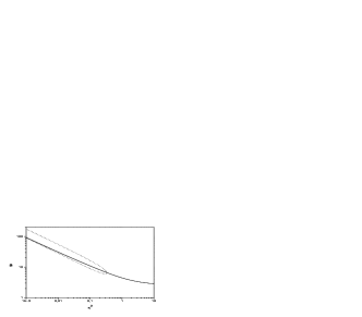
Figure 5: Evolution of shooting parameters (on the left) and of eigenvalues (on the right) for solutions $\mathrm{S}_{\scriptscriptstyle{{1}}}\mathrm{H}_{\scriptscriptstyle{{1}}}\mathrm{S}_{\scriptscriptstyle{{1}}}$ (——-) and $\mathrm{S}_{\scriptscriptstyle{{2}}}\mathrm{S}_{\scriptscriptstyle{{1}}}$ $(\cdots\cdots)$. Instead of eigenvalues here are given the values $\lambda/L$. Here is also introduced the variable $\kappa^{2}:=2/L^{2}$. Solutions $\mathrm{S}_{\scriptscriptstyle{{n}}}\mathrm{H}_{\scriptscriptstyle{{1}}}\mathrm{S}_{\scriptscriptstyle{{n}}}$ with $n\geq 2$ possess qualitatively similar in behaviour spectrum, that is for some critical $L$ the lowest eigenvalue of $\mathrm{S}_{\scriptscriptstyle{{n}}}\mathrm{H}_{\scriptscriptstyle{{1}}}\mathrm{S}_{\scriptscriptstyle{{n}}}$ becomes negative and this is associated with the bifurcation of the new stable solution $\mathrm{S}_{\scriptscriptstyle{{n+1}}}\mathrm{S}_{\scriptscriptstyle{{n}}}$.

For a fixed $n\geq 1$ (this is also true for $n=0$, i.e. $\mathrm{H}_{\scriptscriptstyle{{1}}}$ & $\mathrm{S}_{\scriptscriptstyle{{1}}}$ – the case which was already analysed) the transition between the stable and the unstable stage of the solution $\mathrm{S}_{\scriptscriptstyle{{n}}}\mathrm{H}_{\scriptscriptstyle{{1}}}\mathrm{S}_{\scriptscriptstyle{{n}}}$ is accompanied by the appearance of the pure skyrmionic solution $\mathrm{S}_{\scriptscriptstyle{{n+1}}}\mathrm{S}_{\scriptscriptstyle{{n}}}$, together with $\mathrm{S}_{\scriptscriptstyle{{n}}}\mathrm{S}_{\scriptscriptstyle{{n+1}}}$, which are not reflection symmetric solutions and have positive definite Hessian – thus are stable. As an example in figure 5 are shown characteristics of the solution $\mathrm{S}_{\scriptscriptstyle{{1}}}\mathrm{H}_{\scriptscriptstyle{{1}}}\mathrm{S}_{\scriptscriptstyle{{1}}}$. For $L>L^{*}_{n}$ the solution $\mathrm{S}_{\scriptscriptstyle{{n}}}\mathrm{H}_{\scriptscriptstyle{{1}}}\mathrm{S}_{\scriptscriptstyle{{n}}}$ inherits its single instability from the harmonic map $\mathrm{h}_{\scriptscriptstyle{{1}}}$ to which, between the poles, it pointwise tends as $L\to\infty$. For all $n$ the limiting spectrum is reproduced by eigenvalues of $\mathrm{H}_{\scriptscriptstyle{{1}}}$.

The critical behaviour of solutions $\mathrm{S}_{\scriptscriptstyle{{n}}}\mathrm{H}_{\scriptscriptstyle{{1}}}\mathrm{S}_{\scriptscriptstyle{{n}}}$ is quite analogous to the behaviour of the identity $\mathrm{H}_{\scriptscriptstyle{{1}}}$. In particular, due to the transition in instability at the critical $L^{*}_{n}$ new solutions $\mathrm{S}_{\scriptscriptstyle{{n+1}}}\mathrm{S}_{\scriptscriptstyle{{n}}}$ and its reflection $\mathrm{S}_{\scriptscriptstyle{{n}}}\mathrm{S}_{\scriptscriptstyle{{n+1}}}$, both with spontaneously broken reflection symmetry, appear by bifurcation from $\mathrm{S}_{\scriptscriptstyle{{n}}}\mathrm{H}_{\scriptscriptstyle{{1}}}\mathrm{S}_{\scriptscriptstyle{{n}}}$. In more detail it is described in the next paragraph.

4.4 Symmetric solutions $\mathrm{S}_{\scriptscriptstyle{{n}}}\mathrm{H}_{\scriptscriptstyle{{2k+1}}}\mathrm{S}_{\scriptscriptstyle{{n}}}$ of parity $(-1)$, $\mathrm{S}_{\scriptscriptstyle{{n}}}\mathrm{H}_{\scriptscriptstyle{{2k}}}\overline{\mathrm{S}}_{\scriptscriptstyle{{n}}}$ of parity $(+1)$, and accompanying solutions, $n\geq 0$, $k\geq 1$, (thus also stable pure skyrmionic solutions $\mathrm{S}_{\scriptscriptstyle{{n}}}\overline{\mathrm{S}}_{\scriptscriptstyle{{n}}}$ of parity $(+1)$ and unstable pure harmonic solutions of parity $(\pm 1)$)

The analogous critical phenomenon, by which the solution $\mathrm{S}_{\scriptscriptstyle{{1}}}$ was born by instability of $\mathrm{H}_{\scriptscriptstyle{{1}}}$, we come across by observing the evolution of the reflection symmetric solutions $\mathrm{S}_{\scriptscriptstyle{{n}}}\mathrm{H}_{\scriptscriptstyle{{2k-1}}}\mathrm{S}_{\scriptscriptstyle{{n}}}$ and $\mathrm{S}_{\scriptscriptstyle{{n}}}\mathrm{H}_{\scriptscriptstyle{{2k}}}\overline{\mathrm{S}}_{\scriptscriptstyle{{n}}}$. This instability is responsible for the appearance of new solutions by bifurcations. Unfortunately, unlike in the case of $\mathrm{S}_{\scriptscriptstyle{{1}}}$, these instabilities can not be analyzed here analytically since all solutions but $\mathrm{H}_{\scriptscriptstyle{{1}}}(=\mathrm{S}_{\scriptscriptstyle{{0}}}\mathrm{H}_{\scriptscriptstyle{{1}}}\mathrm{S}_{\scriptscriptstyle{{0}}})$ are known only numerically.

A solution $\mathrm{S}_{\scriptscriptstyle{{n}}}\mathrm{H}_{\scriptscriptstyle{{2k}}}\overline{\mathrm{S}}_{\scriptscriptstyle{{n}}}$, $n\geq 0$, $k\geq 1$ (with eigenvalues $\lambda_{l}=:\alpha_{n,l}$) appears together with $\mathrm{S}_{\scriptscriptstyle{{n+1}}}\overline{\mathrm{H}}_{\scriptscriptstyle{{2k-2}}}\overline{\mathrm{S}}_{\scriptscriptstyle{{n+1}}}$ ($\lambda_{l}=:\beta_{n,l}$) at some characteristic $L:=L_{n,2k}$ when $\alpha_{n,2k-2}=0=\beta_{2k-2}$. Both solutions are of parity $+1$. (If $k=1$ the last solution is simply $\mathrm{S}_{\scriptscriptstyle{{n+1}}}\overline{\mathrm{S}}_{\scriptscriptstyle{{n+1}}}$ thus is pure skyrmionic solution). For $L>L_{n,2k}$ the solution $\mathrm{S}_{\scriptscriptstyle{{n+1}}}\overline{\mathrm{H}}_{\scriptscriptstyle{{2k-2}}}\overline{\mathrm{S}}_{\scriptscriptstyle{{n+1}}}$ has $2k-2$ modes of instability, which is the same as the number of instabilities of the harmonic map $\mathrm{h}_{\scriptscriptstyle{{2k-2}}}$. Moreover, $\alpha_{n,l}<\beta_{n,l}$ for $L>L_{n,2k}$. For $L_{n,2k}<L<L^{*}_{n,2k}$ the eigenvalue $\alpha_{n,2k-1}$ is positive, tends to $0$ as $L\to L^{*}_{n,2k}$ and is negative for $L>L^{*}_{n,2k}$. Thus, for $L>L^{*}_{n,2k}$ $\mathrm{S}_{\scriptscriptstyle{{n}}}\mathrm{H}_{\scriptscriptstyle{{2k}}}\overline{\mathrm{S}}_{\scriptscriptstyle{{n}}}$ has $2k$ modes of instability – the same as the number of modes of the harmonic map $\mathrm{h}_{\scriptscriptstyle{{2k}}}$. At the critical $L^{*}_{n,2k}$ the solution $\mathrm{S}_{\scriptscriptstyle{{n+1}}}\overline{\mathrm{H}}_{\scriptscriptstyle{{2k-1}}}\overline{\mathrm{S}}_{\scriptscriptstyle{{n}}}$ and, due to reflection symmetry, the solution $\mathrm{S}_{\scriptscriptstyle{{n}}}\mathrm{H}_{\scriptscriptstyle{{2k-1}}}\overline{\mathrm{S}}_{\scriptscriptstyle{{n+1}}}$ appear by bifurcation from the solution $\mathrm{S}_{\scriptscriptstyle{{n}}}\mathrm{H}_{\scriptscriptstyle{{2k}}}\overline{\mathrm{S}}_{\scriptscriptstyle{{n}}}$. As an example in figure 6 are presented parameters of the solutions $\mathrm{H}_{\scriptscriptstyle{{2}}}$, $\mathrm{S}_{\scriptscriptstyle{{1}}}\mathrm{S}_{\scriptscriptstyle{{1}}}$ and $\mathrm{S}_{\scriptscriptstyle{{1}}}\overline{\mathrm{H}}_{\scriptscriptstyle{{1}}}$.

Figure 6: The evolution of shooting parameters and eigenvalues for solutions $\mathrm{H}_{\scriptscriptstyle{{2}}}$ (——-), $\mathrm{S}_{\scriptscriptstyle{{1}}}\mathrm{S}_{\scriptscriptstyle{{1}}}$ ($\cdots\cdots$), and $\mathrm{S}_{\scriptscriptstyle{{1}}}\overline{\mathrm{H}}_{\scriptscriptstyle{{1}}}$ (with its partner $\mathrm{H}_{\scriptscriptstyle{{1}}}\overline{\mathrm{S}}_{\scriptscriptstyle{{1}}}$ ) (——-). This is a particular case of more general situation when $\mathrm{S}_{\scriptscriptstyle{{n}}}\mathrm{H}_{\scriptscriptstyle{{2k}}}\overline{\mathrm{S}}_{\scriptscriptstyle{{n}}}$ ($n\geq 0$, $k\geq 1$), together with $\mathrm{S}_{\scriptscriptstyle{{n+1}}}\overline{\mathrm{H}}_{\scriptscriptstyle{{2k-2}}}\overline{\mathrm{S}}_{\scriptscriptstyle{{n+1}}}$ appear and, due to the transition in the number of instabilities of $\mathrm{S}_{\scriptscriptstyle{{n}}}\mathrm{H}_{\scriptscriptstyle{{2k}}}\overline{\mathrm{S}}_{\scriptscriptstyle{{n}}}$, the solution $\mathrm{S}_{\scriptscriptstyle{{n+1}}}\overline{\mathrm{H}}_{\scriptscriptstyle{{2k-1}}}\overline{\mathrm{S}}_{\scriptscriptstyle{{n}}}$ appears by the process of bifurcation. All the solutions have vanishing topological charge.

The solutions $\mathrm{S}_{\scriptscriptstyle{{n}}}\mathrm{H}_{\scriptscriptstyle{{2k}}}\overline{\mathrm{S}}_{\scriptscriptstyle{{n}}}$, $n\geq 0$, $k\geq 1$ and $\mathrm{S}_{\scriptscriptstyle{{n+1}}}\overline{\mathrm{H}}_{\scriptscriptstyle{{2k-2}}}\overline{\mathrm{S}}_{\scriptscriptstyle{{n+1}}}$ differ by $2$ in the number of negative eigenvalues if $L$ is sufficiently large. This is the first solution which possesses $2$ modes of instabilities more than the second solution, and which ’bears’ the new solution. The new solution has $2k-1$ modes of instability (the same as the map $\mathrm{h}_{\scriptscriptstyle{{2k-1}}}$) and is nonsymmetric, unlike the one from which it bifurcates.

The solution $\mathrm{S}_{\scriptscriptstyle{{n}}}\mathrm{H}_{\scriptscriptstyle{{2k+1}}}\mathrm{S}_{\scriptscriptstyle{{n}}}$, with eigenvalues $\lambda_{l}=:\alpha^{\prime}_{n,l}$, appears together with $\mathrm{S}_{\scriptscriptstyle{{n+1}}}\overline{\mathrm{H}}_{\scriptscriptstyle{{2k-1}}}\mathrm{S}_{\scriptscriptstyle{{n+1}}}$, whose eigenvalues are $\lambda_{l}:=\beta^{\prime}_{n,l}$, at some characteristic $L=L_{n,2k+1}$ at which $\alpha^{\prime}_{n,2k-1}=0=\beta^{\prime}_{n,2k-1}$ (figure 7).

Figure 7: Evolution of eigenvalues for solutions $\mathrm{H}_{\scriptscriptstyle{{3}}}$ (——-), $\mathrm{S}_{\scriptscriptstyle{{1}}}\overline{\mathrm{H}}_{\scriptscriptstyle{{1}}}\mathrm{S}_{\scriptscriptstyle{{1}}}$ ($\cdots\cdots$), and $\mathrm{S}_{\scriptscriptstyle{{1}}}\overline{\mathrm{H}}_{\scriptscriptstyle{{2}}}$ ($\mathrm{H}_{\scriptscriptstyle{{2}}}\overline{\mathrm{S}}_{\scriptscriptstyle{{1}}}$) (——-) on the left, and to compare with, the same characteristics for $\mathrm{S}_{\scriptscriptstyle{{1}}}\mathrm{H}_{\scriptscriptstyle{{3}}}\mathrm{S}_{\scriptscriptstyle{{1}}}$ (——-), $\mathrm{S}_{\scriptscriptstyle{{2}}}\overline{\mathrm{H}}_{\scriptscriptstyle{{1}}}\mathrm{S}_{\scriptscriptstyle{{2}}}$ ($\cdots\cdots$), and $\mathrm{S}_{\scriptscriptstyle{{2}}}\overline{\mathrm{H}}_{\scriptscriptstyle{{2}}}\mathrm{S}_{\scriptscriptstyle{{1}}}$. Instead of eigenvalues $\lambda$, are shown $\lambda/L$, here is used also the variable $\kappa^{2}=2/L^{2}$. Both figures are misleadingly similar, note the difference between the critical values of $\kappa^{2}$ and tiny differences between the critical values of eigenvalues in both figures. Because of this one would have the impression that the presence of skyrmions has not very crucial influence on the stability, but it suffices to compare this with the spectrum of $\mathrm{S}_{\scriptscriptstyle{{1}}}\mathrm{H}_{\scriptscriptstyle{{3}}}$ (figure 3) – which is not a symmetric solution – to see this is not the case. These solutions are the particular case of the more general situation when $\mathrm{S}_{\scriptscriptstyle{{n}}}\mathrm{H}_{\scriptscriptstyle{{2k+1}}}\mathrm{S}_{\scriptscriptstyle{{n}}}$ ($n\geq 0$, $k\geq 1$) together with $\mathrm{S}_{\scriptscriptstyle{{n+1}}}\overline{\mathrm{H}}_{\scriptscriptstyle{{2k-1}}}\mathrm{S}_{\scriptscriptstyle{{n+1}}}$ appear and, due to the transition in the number of instabilities of $\mathrm{S}_{\scriptscriptstyle{{n}}}\mathrm{H}_{\scriptscriptstyle{{2k+1}}}\mathrm{S}_{\scriptscriptstyle{{n}}}$ the solutions $\mathrm{S}_{\scriptscriptstyle{{n+1}}}\overline{\mathrm{H}}_{\scriptscriptstyle{{2k}}}\mathrm{S}_{\scriptscriptstyle{{n}}}$ (and $\mathrm{S}_{\scriptscriptstyle{{n}}}\mathrm{H}_{\scriptscriptstyle{{2k}}}\mathrm{S}_{\scriptscriptstyle{{n+1}}}$) appear by the process of bifurcation. These solutions are topologically nontrivial $\mathcal{Q}=2n+1$.

These solutions have also definite parity, i.e. $(-1)$. For $L>L_{n,2k+1}$ the solution $\mathrm{S}_{\scriptscriptstyle{{n+1}}}\overline{\mathrm{H}}_{\scriptscriptstyle{{2k-1}}}\mathrm{S}_{\scriptscriptstyle{{n+1}}}$ has $2k-1$ modes of instability, which is the same as the number of instabilities of the harmonic map $\mathrm{h}_{\scriptscriptstyle{{2k-1}}}$. Moreover $\alpha^{\prime}_{n,l}<\beta^{\prime}_{n,l}$ for $L>L_{n,2k+1}$. For $L_{n,2k+1}<L<L^{*}_{n,2k+1}$ the eigenvalue $\alpha^{\prime}_{n,2k}$ is positive, tends to $0$ as $L\to L^{*}_{n,2k+1}$ and is negative for $L>L^{*}_{n,2k+1}$. Thus, for $L>L^{*}_{n,2k+1}$ the solution $\mathrm{S}_{\scriptscriptstyle{{n}}}\mathrm{H}_{\scriptscriptstyle{{2k+1}}}\mathrm{S}_{\scriptscriptstyle{{n}}}$ has $2k+1$ modes of instability – the same as the number of instabilities of the harmonic map $\mathrm{h}_{\scriptscriptstyle{{2k+1}}}$. This is the critical value $L^{*}_{n,2k+1}$ at which the solution $\mathrm{S}_{\scriptscriptstyle{{n+1}}}\overline{\mathrm{H}}_{\scriptscriptstyle{{2k}}}\mathrm{S}_{\scriptscriptstyle{{n}}}$ (and $\mathrm{S}_{\scriptscriptstyle{{n}}}\mathrm{H}_{\scriptscriptstyle{{2k}}}\mathrm{S}_{\scriptscriptstyle{{n+1}}}$) appear by bifurcation from $\mathrm{S}_{\scriptscriptstyle{{n}}}\mathrm{H}_{\scriptscriptstyle{{2k+1}}}\mathrm{S}_{\scriptscriptstyle{{n}}}$, i.e. from this one of the original pair, which has $2$ more, than the second, modes of instability. The new solutions have constant number of $2k$ modes of instability (the same as $\mathrm{h}_{\scriptscriptstyle{{2k}}}$) and have spontaneously broken parity.

5 The mechanism of the spontaneous breaking of the reflection symmetry

The instabilities described above are closely related to the breaking of reflection symmetry. As the rule we state that solutions which bifurcate from symmetric solutions are not symmetric and that only the solutions which are symmetric turn out ’to be able to give birth’ to new solutions. The special class of hedgehog solutions is described by the reflection symmetric equation (1.2), but some solutions possess no definite parity. This phenomenon is known as the spontaneous breaking of reflection symmetry or of parity. In the case of the Skyrme model on $\mathcal{S}^{3}$ the following reflection symmetries of equation (1.2) are being spontaneously broken: $F(x)\to F(-x)$ and $F(x)\to\mathcal{Q}\pi-F(-x)$ (we assume $\lim_{x\to-\infty}F(x)=0$). We used here the variable $x=\ln{\tan{(\psi/2)}}$. The second symmetry is a composition of several primitive symmetries. Because of this we ascribe a definite parity $+1$ or $-1$ to a solution which is invariant with respect to the first or with respect to the second transformation. By examining the process of the appearance of $\mathrm{S}_{\scriptscriptstyle{{1}}}$ by bifurcation from $\mathrm{H}_{\scriptscriptstyle{{1}}}$, which was performed analytically, the phenomenon of spontaneous breaking of the reflection symmetry can be understood. By comparison with numerical data of other solutions we can generalize our observations. As it will be shown, the explanation of the symmetry breaking can be successfully carried out with the use of the modes whose eigenvalues vanish at some critical radii. This construction follows straightforwardly from the analytical approach of §3.3. Here it should be noted that the first time the wording ’spontaneous breaking of full rotational symmetry’ in the case of Skyrme model on $\mathcal{S}^{3}$ was used, was in the paper [6].

By a critical mode we will call the mode to which it correspond the eigenvalue which vanishes at some critical $L=L^{*}$. We observed that for $L<L^{*}$ this eigenvalue is positive and negative for $L>L^{*}$ in all cases. It is worth to note the fact that a critical mode has always definite parity at least for $L=L^{*}$. This is because the solutions that ’give birth’ to other solutions by bifurcations have definite parity, and we observed that only such solutions possess critical modes. The symmetry of the Sturm-Liouville equation (2.4), which determines these modes for such solutions, can be broken only by the weight function which can be arbitrary. In fact, the vanishing of an eigenvalue means that the corresponding eigenfunction is not affected by the weight function, and by this is intimately connected with the Hessian alone and consequently with the equation (1.2). Thus, by analogy with §3.3 and by the observation of similar behaviour of shooting parameters in the vicinity of critical points $L^{*}_{n,p}$, at which new solutions appear by bifurcations, we can write down the formulas that describe, in the first approximation, the shooting parameters of solutions $\mathrm{S}_{\scriptscriptstyle{{n+1}}}\overline{\mathrm{H}}_{\scriptscriptstyle{{2k-1}}}\overline{\mathrm{S}}_{\scriptscriptstyle{{n}}}$ and $\mathrm{S}_{\scriptscriptstyle{{n}}}\mathrm{H}_{\scriptscriptstyle{{2k-1}}}\overline{\mathrm{S}}_{\scriptscriptstyle{{n+1}}}$ (which bifurcate from $\mathrm{S}_{\scriptscriptstyle{{n}}}\mathrm{H}_{\scriptscriptstyle{{2k}}}\overline{\mathrm{S}}_{\scriptscriptstyle{{n}}}$) or $\mathrm{S}_{\scriptscriptstyle{{n+1}}}\overline{\mathrm{H}}_{\scriptscriptstyle{{2k}}}\mathrm{S}_{\scriptscriptstyle{{n}}}$ and $\mathrm{S}_{\scriptscriptstyle{{n}}}\mathrm{H}_{\scriptscriptstyle{{2k}}}\mathrm{S}_{\scriptscriptstyle{{n+1}}}$ (which bifurcate from $\mathrm{S}_{\scriptscriptstyle{{n}}}\mathrm{H}_{\scriptscriptstyle{{2k+1}}}\mathrm{S}_{\scriptscriptstyle{{n}}}$). For sufficiently small $L>L^{*}_{n,p}$ these formulas read respectively $\mathrm{S}_{\scriptscriptstyle{{n}}}\mathrm{H}_{\scriptscriptstyle{{2k}}}\overline{\mathrm{S}}_{\scriptscriptstyle{{n}}}\pm\gamma_{n,2k}\xi_{n,2k-1}$ or $\mathrm{S}_{\scriptscriptstyle{{n}}}\mathrm{H}_{\scriptscriptstyle{{2k+1}}}\mathrm{S}_{\scriptscriptstyle{{n}}}\pm\gamma_{n,2k+1}\xi_{n,2k}$ where $\xi_{n,p}$ is the critical mode and the coefficient $\gamma_{n,p}$ shows the characteristic for critical phenomena rational power dependence on $(L-L^{*}_{n,p})$ (the exponent was calculated in §(3.3) to be exactly $1/2$ and with very good accuracy this value was also derived by fitting curves to numerical data for several solutions). Note also, that the mode $\xi_{n,2k-1}$ has an odd number of nodal points (hence the parity $-1$) while the solution $\mathrm{S}_{\scriptscriptstyle{{n}}}\mathrm{H}_{\scriptscriptstyle{{2k}}}\overline{\mathrm{S}}_{\scriptscriptstyle{{n}}}$ has parity $+1$. Analogously $\xi_{n,2k}$ has parity $+1$ which is opposite to the parity of $\mathrm{S}_{\scriptscriptstyle{{n}}}\mathrm{H}_{\scriptscriptstyle{{2k+1}}}\mathrm{S}_{\scriptscriptstyle{{n}}}$. Thus, the solutions which appear by bifurcation process have indefinite parity, i.e. have spontaneously broken reflection symmetry. In the first approximation, it is due to the excitation of the critical mode which has the opposite parity with respect to the parity of the excited reflection symmetric solution. This occurs while the qualitative transition takes place, when the reflection symmetric solution undergoes increase by $1$ in its number of instabilities. In other words, one can say that at the critical point, in a sense, it costs no energy of the excitation of the critical mode. This is always inevitably connected with the process of spontaneous breaking of reflection symmetry.

6 Conclusions

In this paper the linear stability analysis of the whole spectrum of the Skyrme’s hedgehogs on the three-sphere was carried out.We considered only spherically symmetric perturbations. The most remarkable it proved the influence of instability modes on the existence of a class of solutions with spontaneously broken parity and which appeared by a critical phenomenon. Also some general remarks on the construction of the Hilbert space of admissible perturbations were presented together with the resulting problem of a choice of a norm and its influence on the resulting spectrum of perturbations.

The main lesson of this paper is that for $L$ sufficiently large ($L$ is interpreted as the radius of the base three-sphere) the number of instabilities of solutions $\mathrm{S}_{\scriptscriptstyle{{n}}}\mathrm{H}_{\scriptscriptstyle{{k}}}\overline{\mathrm{S}}_{\scriptscriptstyle{{m}}}$ is the same as the index of the harmonic map $\mathrm{h}_{\scriptscriptstyle{{k}}}$ to which (apart from the poles) the solutions tend pointwise as the radius grows. The appearance of new solutions is always accompanied by the vanishing of some eigenvalue of the spectrum of the Hessian. In particular, pure skyrmionic solutions $\mathrm{S}_{\scriptscriptstyle{{n}}}\mathrm{S}_{\scriptscriptstyle{{m}}}$ localized at the poles are always linearly stable. The number of instabilities of nonsymmetric solutions is independent on $L$. There also exist a class of reflection symmetric solutions whose number of negative modes increase by one as $L$ grows. Due to the qualitative transition new solutions with broken reflection symmetry appear by bifurcations and this process possesses many characteristics of a critical phenomenon. In particular, the identity solution $\mathrm{H}_{\scriptscriptstyle{{1}}}$, which is stable for small $L$, becomes unstable at $L=\sqrt{2}$. Then the $1$-skyrmion $\mathrm{S}_{\scriptscriptstyle{{1}}}$ (together with its reflections) is born by biffurcation from the $\mathrm{H}_{\scriptscriptstyle{{1}}}$ and exists as a stable solution for $L>\sqrt{2}$. In this unique case the critical phenomenon may be astonishingly simply described analytically and therefore completely understood. This gives rise to a general picture of the process of the spontaneous breaking of the reflection symmetry which may be intuitively presented as a costing no energy inflation of the critical mode on the unstable symmetric solution. The unstable solution and the critical mode have mutually opposite parity, thus the newly born solution has spontaneously broken parity. Finnaly, we also found two unique series expansions for the profile and for the energy of the $1$-skyrmion (although the respective expansion coefficients are not known in general forms) which read respectively

$$F(\psi)=\psi+x\sin{\psi}+x^{2}\frac{3}{20}\sin{2\psi}-x^{3}\left(\frac{29369}{316800}\sin{\psi}-\frac{11}{480}\sin{3\psi}\right)$$

$$\qquad\qquad\qquad-x^{4}\left(\frac{4217}{887040}\sin{2\psi}-\frac{109}{20160}\sin{4\psi}\right)+\dots$$

and

$$\frac{E[F]}{12\pi^{2}}=\frac{3\sqrt{2}}{4}\left(1+\frac{11}{180}x^{2}-\frac{209}{10800}x^{4}+\frac{5209}{864000}x^{6}-\frac{2126641283}{1149603840000}x^{8}+\mathcal{O}{(x^{10})}\right),$$

where

$$x=\pm\sqrt{\frac{60}{11}\left(\frac{L}{\sqrt{2}}-1\right)}.$$

These series expansions are valid in some right neighbourhood of the critical radius $L=\sqrt{2}$ and numerical assessment of their behaviour makes them plausible to possesss nonzero radii of convergence.

This critical behaviour which we observed in our model exist neither in the Skyrme model on the flat space nor in the model of harmonic maps between three-spheres when free parameters of these models – the characteristic size of a soliton in the first case, or the radius of the base three-sphere in the second case – are being changed. It shows that by coupling together two field theories we may produce another theory in which new phenomena may appear that are absent in the decoupled case. Dimensional parameters introduced by different models determine then some dimensionless numbers whose values are usually crucial to the existence of different types of solutions. This fact is known when nonlinear fields are coupled to gravity [2]. The main motivation of our work was to understand such model-independent phenomena in possibly the simplest case which is a nonlinear scalar field theory on a fixed space-time background.

Appendix A Formal series expansion for the profile and energy of the skyrmion $\mathrm{S}_{\scriptscriptstyle{{1}}}$ on $\mathcal{S}^{3}$

In order to find a formal series expansion for the profile $F(\psi)$ of $\mathrm{S}_{\scriptscriptstyle{{1}}}$ in the vicinity of $L=\sqrt{2}$ we assume that this solution can be written using the following ansatz:

$$F(\psi,x)=\psi$$ (A.1)

$$+\left\{a_{1}+x^{2}a_{3}\left(1+a_{3,3}\frac{\sin{3\psi}}{\sin{\psi}}\right)+x^{4}a_{5}\left(1+a_{5,3}\frac{\sin{3\psi}}{\sin{\psi}}+a_{5,5}\frac{\sin{5\psi}}{\sin{\psi}}\right)+\dots\ \right\}$$

$$\qquad\cdot x\sin{\psi}$$

$$+\left\{a_{2}+x^{2}a_{4}\left(1+a_{4,4}\frac{\sin{4\psi}}{\sin{2\psi}}\right)+x^{4}a_{6}\left(1+a_{6,4}\frac{\sin{4\psi}}{\sin{2\psi}}+a_{6,6}\frac{\sin{6\psi}}{\sin{2\psi}}\right)+\dots\ \right\}$$

$$\qquad\cdot x^{2}\sin{2\psi}$$

where

$$x=\sqrt{\frac{60}{11}\left(\frac{L}{\sqrt{2}}-1\right)},\qquad L>\sqrt{2},\quad\mathrm{and}\quad a_{1}:=1.$$

This ansatz follows from the idea that the solution $F(\psi,x)$ should be linearly decomposed in the base of eigenfunctions of the Hessian (2.1) evaluated at $\mathrm{H}_{\scriptscriptstyle{{1}}}$. This is implied by the appearance of $\mathrm{S}_{\scriptscriptstyle{{1}}}$ at the critical radius $L=\sqrt{2}$ by the excitation of the lowest energy mode (i.e. $\sin{\psi}$) on $\mathrm{H}_{\scriptscriptstyle{{1}}}$, which was perfectly confirmed when we reproduced analytically the numerical observation that

$$|a-1|=\sqrt{\frac{30\sqrt{2}}{11}\left(L-\sqrt{2}\right)}:=x,$$

which implies that

$$\frac{\partial F(\psi,x)}{\partial{x}}\bigg{|}_{x=0}=\sin{\psi},$$

and the vague idea that this behaviour should be somehow analytically continued in the variable $x$. From the symmetry of equation (1.2) we impose on the series also the requirement that, since $L\propto x^{2}$, the second solution $\pi-F(\pi-\psi,x)$ should be simply $F(\psi,-x)$ (both skyrmions bifurcate from $\mathrm{H}_{\scriptscriptstyle{{1}}}$ at $x=0$ and can be transformed one to another by the reflection with respect to the point $(\pi/2,\pi/2)$).

The coefficients $a_{k}$ and $a_{k,l}$ (at least the one we had found) are rational numbers and relations between them become more and more complicated as $k$ increases. Due to nonlinearity of equation (1.2) it seems there is no general recurrence which would determine these coefficients. Anyway, the above ansatz enables us to find them all successively step by step. In table 1 we give all the coefficients which are required to determine the profile of $\mathrm{S}_{\scriptscriptstyle{{1}}}$ with the accuracy up to $\mathcal{O}{(x^{14})}$. The question arises if the formal series possesses nonzero radius of convergence. We gave in the main text some arguments that this series is really a solution. In order to enhance our argumentation we may try to estimate this radius. We can treat the maximal absolute values of the functional coefficients standing in braces at $x^{2k}$ in equation (A.1) to built a majorizing power series in the variable $x$. Let denote the respective values by $\{c_{1},c_{3},\dots\}$ and $\{c_{2},c_{4},\dots\}$ respectively for the first and the second brace. Thus the partial sums of the above series are majorized by $\sum c_{n}|x|^{n}$. In figure 8

Figure 8:
left: Initial elements of the sequence $\{1/\sqrt[n]{c_{n}}\}$, where $\sum_{n}c_{n}x^{n}$ is a majorizing series for the profile of $\mathrm{S}_{\scriptscriptstyle{{1}}}$. This strongly suggest that the Taylor-Fourier series expansion (A.1) has a nonzero radius of convergence and even that, it is absolutely convergent.
right: Initial elements of the sequence $\{1/\sqrt[2n]{d_{2n}}\}$ where $d_{2n}$ are defined in (A.2). This suggest that the Taylor series expansion of energy of $\mathrm{S}_{\scriptscriptstyle{{1}}}$ may have a nonzero radius of convergence.

are shown $20$ initial elements of the sequence $(1/\sqrt[n]{c_{n}})$. Their behaviour strongly suggest the hypothesis that the Taylor-Fourier series expansion (A.1) has a nonzero radius of convergence and even that, it is absolutely convergent.

$a_{1}=1$	$a_{2}=+\frac{3}{20}$
$a_{3}=-\frac{29369}{316800}$	$a_{4}=-\frac{4217}{887040}$
$a_{3,3}=-\frac{7260}{29369}$	$a_{4,4}=-\frac{4796}{4217}$
$a_{5}=+\frac{12335768813}{1405071360000}$	$a_{6}=+\frac{5010043861}{7376624640000}$
$a_{5,3}=-\frac{4404867060}{12335768813}$	$a_{6,4}=-\frac{33475541308}{5010043861}$
$a_{5,5}=+\frac{3226815900}{12335768813}$	$a_{6,6}=+\frac{13362918261}{10020087722}$
$a_{7}=+\frac{7986485836639}{25751126016000000}$	$a_{8}=-\frac{473077794653026103}{98150416809984000000}$
$a_{7,3}=+\frac{158986289932080}{7986485836639}$	$a_{8,4}=-\frac{361662885996135944}{473077794653026103}$
$a_{7,5}=-\frac{57715917199500}{7986485836639}$	$a_{8,6}=+\frac{51442637682491484}{473077794653026103}$
$a_{7,7}=+\frac{6755487649680}{7986485836639}$	$a_{8,8}=-\frac{5773312055063520}{473077794653026103}$
$a_{9}=-\frac{127577656118454895711}{167510044689039360000000}$	$a_{10}=+\frac{4211381544228526601549071}{1061084526049375027200000000}$
$a_{9,3}=+\frac{790229840916734772664}{127577656118454895711}$	$a_{10,4}=-\frac{822641146563016022074558}{4211381544228526601549071}$
$a_{9,5}=-\frac{309555559736002696600}{382732968355364687133}$	$a_{10,6}=-\frac{1447811040980803898316621}{33691052353828212812392568}$
$a_{9,7}=+\frac{20023176097891467424}{382732968355364687133}$	$a_{10,8}=-\frac{13895432790539792801760}{4211381544228526601549071}$
$a_{9,9}=-\frac{2544822818150368800}{127577656118454895711}$	$a_{10,10}=+\frac{55236971873923883695575}{33691052353828212812392568}$
$a_{11}=+\frac{982955548821103176200169976183}{2390411220284032061276160000000000}$	$a_{12}=-\frac{107845172239555936226487785603477}{73415504602973334681944064000000000}$
$a_{11,3}=+\frac{3024748425995528913667880277780}{982955548821103176200169976183}$	$a_{12,4}=+\frac{60201002753190711583565881906936}{107845172239555936226487785603477}$
$a_{11,5}=+\frac{1248755928443601042244324285400}{982955548821103176200169976183}$	$a_{12,6}=-\frac{8388700062249632787593687120376}{107845172239555936226487785603477}$
$a_{11,7}=-\frac{58074313732006509362657835680}{982955548821103176200169976183}$	$a_{12,8}=-\frac{5165826035166448141662612158400}{107845172239555936226487785603477}$
$a_{11,9}=-\frac{56310543306011901706414401600}{982955548821103176200169976183}$	$a_{12,10}=+\frac{975465355644891981999033888060}{107845172239555936226487785603477}$
$a_{11,11}=+\frac{6823246116254206530384345600}{982955548821103176200169976183}$	$a_{12,12}=-\frac{68171833635114106739516947272}{107845172239555936226487785603477}$
$a_{13}=-\frac{43153404274707851225466988047569832167}{413476121923945820928708968448000000000000}$	$a_{14}=-\frac{1766865169954398109033856353883942537617}{6132984423523186432660243218432000000000000}$
$a_{13,3}=-\frac{313572180766907863870688164387239391620}{43153404274707851225466988047569832167}$	$a_{14,4}=-\frac{4349592583735535844513687814933733037976}{1766865169954398109033856353883942537617}$
$a_{13,5}=+\frac{137371166634494138333962660336190541100}{43153404274707851225466988047569832167}$	$a_{14,6}=-\frac{1508853846688227478046216373401843325339}{1766865169954398109033856353883942537617}$
$a_{13,7}=+\frac{65940526790056736560082171865362030240}{43153404274707851225466988047569832167}$	$a_{14,8}=+\frac{585277715345242542258046459394514314520}{1766865169954398109033856353883942537617}$
$a_{13,9}=-\frac{16887408629502465138357459627899436000}{43153404274707851225466988047569832167}$	$a_{14,10}=-\frac{78074347310444368596245949472056202125}{3533730339908796218067712707767885075234}$
$a_{13,11}=+\frac{1437225091006557895313712800717160000}{43153404274707851225466988047569832167}$	$a_{14,12}=+\frac{1726765295922525300215513807655077490}{1766865169954398109033856353883942537617}$
$a_{13,13}=-\frac{92252259291662946944254093579272000}{43153404274707851225466988047569832167}$	$a_{14,14}=-\frac{38714472844152751765544208844685625}{199083399431481477074237335648894933816}$

Table 1: Initial coefficients of the Taylor-Fourier series expansion (A.1) of the solution $\mathrm{S}_{\scriptscriptstyle{{1}}}$ in the vicinity of the critical radius $L=\sqrt{2}$.

The Taylor series expansion of the energy of $\mathrm{S}_{\scriptscriptstyle{{1}}}$ around $x=0$ must contain only even powers of $x$ since $F(\psi,x)$ and $F(\psi,-x)$ must have equal energies. Therefore the energy of $\mathrm{S}_{\scriptscriptstyle{{1}}}$ is a smooth function of $L-\sqrt{2}$, unlike the $F^{\prime}(0,x(L))-1$, which has a branch singularity at $L=\sqrt{2}$. This series reads

$$\frac{E(x)}{12\pi^{2}}=\frac{3}{4}\sqrt{2}\left(1+d_{2}x^{2}+d_{4}x^{4}+\dots\right)$$ (A.2)

and the respective coefficients are given in table 2.

$d_{2\ }=+\frac{11}{180}$

$d_{4\ }=-\frac{209}{10800}$

$d_{6\ }=+\frac{5209}{864000}$

$d_{8\ }=-\frac{2126641283}{1149603840000}$

$d_{10}=+\frac{8434513426021}{16995743170560000}$

$d_{12}=-\frac{464402526814953371}{6730314295541760000000}$

$d_{14}=-\frac{23242947675020983465203089}{626856089235323092992000000000}$

$d_{16}=+\frac{14367315331877365555523427348253}{379122562769523406641561600000000000}$

$d_{18}=-\frac{31939951417910304147919969132085999}{2017781268474468255763984809984000000000}$

$d_{20}=-\frac{74250563114418365106618380718783299763796141}{109069148686118907097066434918875136000000000000000}$

Table 2: Initial coefficients of the Taylor series expansion of energy of $\mathrm{S}_{\scriptscriptstyle{{1}}}$ at the critical radius $L=\sqrt{2}$. In order to calculate $d_{2n}$ we need the profile of $\mathrm{S}_{\scriptscriptstyle{{1}}}$ to be determined with the accuracy up to $x^{2n}$.

For $x=0$ we get the energy of $\mathrm{H}_{\scriptscriptstyle{{1}}}$ at $L=\sqrt{2}$. Here we also construct the sequence $\{1/\sqrt[2n]{d_{2n}}\}$ to make it plausible that the series (A.2) and, indirectly, the series (A.1), have nonzero radius of convergence. In figure 8 are shown initial elements of the sequence $(1/\sqrt[2n]{d_{2n}})$. Their behaviour suggest the hypothesis that the Taylor series expansion (A.2) may have a nonzero radius of convergence.

Appendix B On the weight function originating from a kinetic term

In this appendix we derive the formula for the weight function, which naturally follows from the calculus of small oscillations about equilibrium. We obtain this by the comparison of two conceptually different approaches to linear stability analysis. Suppose, for example, that we have a differential equation for a function of one space variable and that the equation is a condition for extrema of some functional. If the function is a solution and, moreover, a local minimum of the functional then it is also a stable equilibrium of some $1+1$ dimensional field theory. Stability is required for physical reasons. In order to check that the function is a minimum it suffices to prove positive definiteness of the second variation of the functional. This in turn requires the existence of a scalar product (which should be defined by additional argumentation) and defines a Sturm-Liouville problem. On the other hand, in linear approximation, the calculus of small oscillations about the equilibrium produces another Sturm-Liouville problem with a definite weight function determined by the kinetic term of the field theory. It turns out that both the problems comprise identical self-adjoint differential operators (the function spaces of admissible perturbations are the same by construction). Thus, to specify the weight function in the first case, it is natural the requirement that both methods should give the same results. Of course, to check positive definiteness of the second variation of the functional we can assume an arbitrary weight function. If the function is not a minimum we are not guaranteed that the different field theories have qualitatively the same dynamics in the vicinity of the common equilibrium. It would be so, under the condition that the number of instable modes were independent of the weight functions, which is not obvious. In what follows we determine the weight function.

We can supplement functional (1.4) with an arbitrary kinetic term not depending explicitly on time (to have the total energy $\mathcal{E}[F(\tau)]$ conserved)

$$\mathcal{E}[F(\tau)]=\int\limits_{0}^{\pi}w(\psi)\left(K(\psi,F(\psi,\tau),\dot{F}(\psi,\tau))+V(\psi,F(\psi,\tau),F^{\prime}(\psi,\tau))\right)\mathrm{d}{\psi},$$

and observe the resulting time-evolution of some initial data in time $\tau$. Conventionally we measure duration using natural units of length $\mathbf{e}^{-1}\mathbf{f}_{\pi}^{-1}$ then $\tau$ is dimensionless. The quantities $K$ and $V$ are interpreted as densities of kinetic and potential energy respectively. We assume that $K=\tilde{K}\dot{F}^{2}$ where $\tilde{K}$ is positive function of $\psi,F,F^{\prime},\dot{F}$. A perturbation can be imagined as a time dependent excess from the equilibrium. An equilibrium solution $F$ is said to be dynamically stable if it remains within some finite bounds $\|{\delta F(\tau)}\|<\varepsilon(\Delta)$ for every $\tau$ if only the initial perturbation is sufficiently small such that $\delta E<\Delta$. Thus, to check stability an initial solution is required to be not arbitrary but such, as its total energy was slightly above the energy of the equilibrium solution and in its pointwise vicinity. It is clear that different kinetic terms give rise to different time evolution and the equilibria are common and the same as solutions of equation (1.2), since the condition that $\delta{\mathcal{U}[F]}/\delta{F(\psi)}=0$ for static solutions is the straightforward consequence of equation of motion

$$\frac{\partial{K}}{\partial{F}}-\frac{\mathrm{d}}{\mathrm{d}{t}}\frac{\partial{K}}{\partial{\dot{F}}}-\frac{\delta{\mathcal{U}[F]}}{\delta{F}}=0$$ (B.1)

and of the requirement that the solutions were in equilibrium. If we had decided to assume the kinetic energy density as in the original Skyrme model on $\mathcal{S}^{3}$, i.e.

$$K(\psi,F,\dot{F})=\left(L+\frac{2}{L}\frac{\sin^{2}{F}}{\sin^{2}{\psi}}\right)L^{2}\dot{F}^{2},$$ (B.2)

then the evolution of the system would have been governed by the equation

$$\left(L\sin^{2}{\psi}+\frac{2}{L}\sin^{2}{F}\right)\left(F^{\prime\prime}-L^{2}\ddot{F}\right)+\frac{1}{L}\sin{2F}\left(F^{\prime 2}-L^{2}\dot{F}^{2}\right)+L\sin{2\psi}F^{\prime}$$

$$-\left(L+\frac{1}{L}\frac{\sin^{2}{F}}{\sin^{2}{\psi}}\right)\sin{2F}=0,$$

while assuming $K(\psi,F,\dot{F})=L^{3}\dot{F}^{2}$ we would have been led to the equation

$$\left(L\sin^{2}{\psi}+\frac{2}{L}\sin^{2}{F}\right)F^{\prime\prime}-\sin^{2}{\psi}L^{3}\ddot{F}+\left(L+\frac{1}{L}\frac{\sin{2F}}{\sin{2\psi}}F^{\prime}\right)\sin{2\psi}F^{\prime}$$

$$-\left(L+\frac{1}{L}\frac{\sin^{2}{F}}{\sin^{2}{\psi}}\right)\sin{2F}=0.$$

As it will turn out the last choice for $K$ gives, up to a constant factor $L^{3}$, the natural on $\mathcal{S}^{3}$ weight function $4\pi\sin^{2}{\psi}$. We can always look for solutions in the form of $F(\psi,\tau)=F(\psi)+\varepsilon\eta(\psi,\tau)$ where $\varepsilon$ measures the scale of perturbation, i.e. its energy, which is proportional to $\varepsilon^{2}$. Next, for small $\varepsilon$ by analogy with the calculus of small oscillations, solutions (if exist) for which $\eta$ is bounded for all $\tau$, may be arbitrarily well approximated by the following linear equation, which is derived by equating with zero the term of the order $\mathcal{O}{(\varepsilon)}$ in the Taylor series expansion of equation (B.1) in the variable $\varepsilon$, i.e.

$$-\left(w\frac{\partial^{2}U}{\partial F^{\prime 2}}\frac{\partial{\eta}}{\partial{\psi}}\right)^{\prime}+\left(w\frac{\partial^{2}U}{\partial F^{2}}-\left(w\frac{\partial^{2}U}{\partial FF^{\prime}}\right)^{\prime}\right)\eta=-w\frac{\partial^{2}K}{\partial\dot{F}^{2}}\frac{\partial^{2}\eta}{\partial\eta^{2}}.$$ (B.3)

Other terms (not shown) which enter above equation vanish since we perturb a static solution for which $\dot{F}=0$. If the equilibrium was not stable the approximation would still have been useful to predict the existence of instabilities. It follows, that for the class of kinetic terms assumed it is always possible to find $\eta$ by the method of separation of variables $\eta(\psi,\tau)=\xi(\psi)\alpha(\tau)$, where $\alpha$ is of the form $\alpha(\tau)=e^{i\omega\tau}$ and $\omega^{2}<0$ for unstable modes. Thus the dynamics impose the natural choice that weight function $g(\psi)$ should be defined according to the formula

$$g(\psi)=w(\psi)\frac{1}{2}\frac{\partial^{2}K}{\partial\dot{F}\partial\dot{F}}\bigg{|}_{F_{equil}},$$ (B.4)

since equation (B.4) reduces to equation (2.3) after the substitution $\eta(\psi,\tau)=\xi(\psi)\sin{(\omega\tau+\phi)}$ with $\lambda=\omega^{2}$ or, if the mode is unstable, $\eta(\psi,\tau)=\xi(\psi)\exp{(\pm\omega\tau)}$ with $\lambda=-\omega^{2}$. Put differently, multiplying (B.3) by $\eta/2$ and integrating, yields

$$\frac{1}{2}\delta^{2}\mathcal{U}[F][\xi]=\lambda\int\limits_{0}^{\pi}w\frac{1}{2}\frac{\partial^{2}K}{\partial\dot{F}\partial\dot{F}}\xi^{2}$$

since $\ddot{\alpha}+\lambda\alpha=0$ which reproduces (2.3) for the special choice of $g$. In this sense, the spectrum of (2.4) with $g=w$ may be interpreted as $\omega^{2}$ for a spherically symmetric scalar field on $\mathcal{S}^{3}$ in an equilibrium if $K=\dot{F}^{2}$. Thus, the Hilbert space spanned on vanishing on boundaries and mutually orthogonal (with respect to the special $g$) eigenfunctions $\xi_{i}$ of the self-adjoint equation (B.3) is constructed and each perturbation $\eta$ is a superposition $\eta(\psi,\tau)=\sum_{k}\xi_{k}(\psi)(a_{k}\alpha_{k}(\tau)+b_{k}\beta_{k}(\tau))$ where $\alpha_{k}$ denotes $\sin{\omega_{k}\tau}$ or $\sinh{\omega_{k}\tau}$ and $\beta_{k}$ denotes $\cos{\omega_{k}\tau}$ or $\cosh{\omega_{k}\tau}$, respectively, if $\lambda_{k}$ is positive or negative. Only a finite number of modes can be unstable. The total energy of the perturbation is finite and quadratic in amplitudes (proportional to $\varepsilon^{2}$) and, of course, only if all $\lambda_{k}$ are positive the function $F(\psi)+\varepsilon\eta(\psi,\tau)$ well approximates the particular solution of equation (B.1) for all $\tau$.

It is thus seen that the linear dynamical stability is closely related to the (abstract) notion of linear energetical stability defined in 2.2.1 and, if the weight function $g$ is appropriately chosen, all eigenvalues of the Hessian $\delta^{2}\mathcal{U}[F][\xi]$ may be directly interpreted as squared eigenfrequencies $\omega_{k}^{2}$ of a system whose dynamics is related to some kinetic term.

References

- [1] Bizoń P 1995 Harmonic maps between three-spheres Proc. R. Soc. A 451 779-93
- [2] Bizoń P and Chmaj T 1992 Gravitating skyrmions Phys. Lett. B 297 55-62
- [3] Bratek Ł 2003 Structure of solutions of the Skyrme model on a three-sphere: numerical results Nonlinearity16 1539-64
- [4] Courant R, Hilbert D 1953 Methods of mathematical physics Vol.I,II
- [5] Lukierski J 1980 Fourdimensional Quaterionic -Models in Field Theoretical Methods in Particle Physics, Ed. by Rühl W (Plenum Press NY) NATO Advanced Study Institutes Series B 55 361
- [6] Manton N S and Ruback P J 1986 Skyrmions in flat space and curved space Phys. Lett. B 181 137-40
- [7] Manton N S 1987 Geometry of Skyrmions Commun. Math. Phys. 111 469-78
- [8] McLeod J B and Troy W C 1991 The Skyrme model for nucleons under spherical symmetry Proc. R. Soc.Edinburgh A 118 271-88
- [9] Skyrme T H R 1961 A non-linear field theory Proc. R. Soc.London A 260 127-38