Mystery of point charges

Abstract.

We discuss the problem of finding an upper bound for the number of equilibrium points of a potential of several fixed point charges in $\mathbb{R}^{n}$. This question goes back to J. C. Maxwell [11] and M. Morse [13]. Using fewnomial theory we show that for a given number of charges there exists an upper bound independent of the dimension, and show it to be at most 12 for three charges. We conjecture an exact upper bound for a given configuration of nonnegative charges in terms of its Voronoi diagram, and prove it asymptotically.

1. Introduction

Consider a configuration of $l=\mu+\nu$ fixed point charges in $\mathbb{R}^{n},\;n\geq 3$ consisting of $\mu$ positive charges with the values $\zeta_{1},\ldots,\zeta_{\mu}$, and $\nu$ negative charges with the values $\zeta_{\mu+1},\ldots,\zeta_{l}$. They create an electrostatic field whose potential equals

(1.1) $$V(\bar{x})=\left(\frac{\zeta_{1}}{r_{1}^{n-2}}+\ldots+\frac{\zeta_{\mu}}{r_{\mu}^{n-2}}\right)+\left(\frac{\zeta_{\mu+1}}{r_{\mu+1}^{n-2}}+\ldots+\frac{\zeta_{l}}{r_{l}^{n-2}}\right),$$

where $r_{i}$ is the distance between the $i$-th charge and the point $\bar{x}=(x_{1},\ldots,x_{n})\in\mathbb{R}^{n}$ which we assume different from the locations of the charges. Below we consider the problem of finding effective upper bounds on the number of critical points of $V(\bar{x})$, i.e. the number of points of equilibrium of the electrostatic force. In what follows we mostly assume that considered configurations of charges have only nondegenerate critical points. This guarantees that the number of critical points is finite. Such configurations of charges and potentials will be called nondegenerate. Surprisingly little is known about this whole topic and the references are very scarce.

In the case of $\mathbb{R}^{3}$ one of the few known results obtained by direct application of Morse theory to $V(\bar{x})$ is as follows, see [13], Theorem 32.1 and [7], Theorem 6.

Theorem 1.1 (Morse-Kiang).

Assume that the total charge $\sum_{i=1}^{l}\zeta_{j}$ in (1.1) is negative (resp. positive). Let $m_{1}$ be the number of the critical points of index $1$ of $V$, and $m_{2}$ be the number of the critical points of index $2$ of $V$. Then $m_{2}\geq\mu$ (resp. $m_{2}\geq\mu-1)$ and $m_{1}\geq\nu-1$ (resp. $m_{1}\geq\nu$). Additionally, $m_{1}-m_{2}=\nu-\mu-1$.

Note that the potential $V(\bar{x})$ has no (local) maxima or minima due to its harmonicity.

Remark. The remaining (more difficult) case $\sum_{i=1}^{\mu}\zeta_{i}+\sum_{j=\mu+1}^{l}\zeta_{j}=0$ is treated in [7].

Remark. The above theorem has a generalization to any $\mathbb{R}^{n},\;$ $n\geq 3$ with $m_{1}$ being the number of the critical points of index $1$ and $m_{2}$ being the number of the critical points of index $n-1$.

Definition 1.2.

Configurations of charges with all nondegenerate critical points and $m_{1}+m_{2}=\mu+\nu+1$ are called minimal, see [13], p. 292.

Remark. Minimal configurations occur if one, for example, places all charges of the same sign on a straight line. On the other hand, it is easy to construct generic nonminimal configurations of charges, see [13].

Remark. The major difficulty of this problem is that the lower bound on the number of critical points of $V_{n}$ given by Morse theory is known to be not exact. Therefore, since we are interested in an effective upper bound, the Morse theory arguments do not provide an answer.

The question about the maximum (if it exists) of the number of points of equilibrium of a nondegenerate configuration of charges in $\mathbb{R}^{3}$ was posed in [13], p. 293. In fact, J. C. Maxwell in [11], section 113 made an explicit claim answering exactly this question.

Conjecture 1.3 ([11], see also §4 below).

The total number of points of equilibrium (all assumed nondegenerate) of any configuration with $l$ charges in $\mathbb{R}^{3}$ never exceeds $(l-1)^{2}$.

Remark. In particular, there are at most $4$ points of equilibrium for any configuration of $3$ point charges according to Maxwell, see Figure 1.

Before formulating our results and conjectures let us first generalize the set-up. In the notation of Theorem 1.1 consider the family of potentials depending on a parameter $\alpha\geq 0$ and given by

(1.2) $$V_{\alpha}(\bar{x})=\left(\frac{\zeta_{1}}{\rho_{1}^{\alpha}}+\ldots+\frac{\zeta_{\mu}}{\rho_{\mu}^{\alpha}}\right)+\left(\frac{\zeta_{\mu+1}}{\rho_{\mu+1}^{\alpha}}+\ldots+\frac{\zeta_{l}}{\rho_{l}^{\alpha}}\right),$$

where $\rho_{i}=r_{i}^{2},\;i=1,\ldots,l$. (The choice of $\rho_{i}$’s instead of $r_{i}$’s is motivated by convenience of algebraic manipulations.)

Notation 1.4.

Denote by $N_{l}(n,\alpha)$ the maximal number of the critical points of the potential (1.2) where the maximum is taken over all nondegenerate configurations with $l$ variable point charges, i.e. over all possible values and locations of $l$ point charges forming a nondegenerate configuration.

Our first result is the following uniform (i.e. independent on $n$ and $\alpha$) upper bound.

Theorem 1.5.

a) For any $\alpha\geq 0$ and any positive integer $n$ one has

(1.3) $$N_{l}(n,\alpha)\leq 4^{l^{2}}(3l)^{2l}.$$

b) For $l=3$ one has a significantly improved upper bound

$$N_{3}(n,\alpha)\leq 12.$$

Remark. Note that the right-hand side of the formula (1.3) gives even for $l=3\;$ the horrible upper bound $139,314,069,504$. On the other hand, computer experiments suggest that Maxwell was right and that for any three charges there are at most 4 (and not $12$) critical points of the potential (1.2), see Figure 1.

         

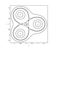
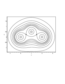
Figure 1. Configurations with two and with four critical points.

Remark. Figure 1 shows the level curves of the restrictions of the potential of three positive charges to the plane they span in two essentially different cases (conjecturally, the only ones). The graph on the left has 3 saddles and 1 local minimum and the graph on the right has just 2 saddle points.

1.1. Voronoi diagrams and the main conjecture

Theorem 1.6 below determines the number of critical points of the function $V_{\alpha}$ for large $\alpha$ in terms of the combinatorial properties of the configuration of the charges. To describe it we need to introduce several notions.

Notation. By a (classical) Voronoi diagram of a configuration of pairwise distinct points (called sites) in the Euclidean space $\mathbb{R}^{n}$ we understand the partition of $\mathbb{R}^{n}$ into convex cells according to the distance to the nearest site, see e.g. [3] and [15].

A Voronoi cell $S$ of the Voronoi diagram consists of all points having exactly the same set of nearest sites. The set of all nearest sites of a given Voronoi cell $S$ is denoted by $\mathcal{NS}(S)$. One can see that each Voronoi cell is a interior of a convex polyhedron, probably of positive codimension. This is a slight generalization of traditional terminology, which considers the Voronoi cells of the highest dimension only.

A Voronoi cell of the Voronoi diagram of a configuration of sites is called effective if it intersects the convex hull of $\mathcal{NS}(S)$.

If we have an additional affine subspace $L\subset\mathbb{R}^{n}$ we call a Voronoi cell $S$ of the Voronoi diagram of a configuration of charges in $\mathbb{R}^{n}$ effective with respect to $L$ if $S$ intersects the convex hull of the orthogonal projection of $\mathcal{NS}(S)$ onto $L$.

A configuration of points is called generic if any Voronoi cell $S$ of its Voronoi diagram of any codimension $k$ has exactly $k+1$ nearest cites and does not intersect the boundary of the convex hull of $\mathcal{NS}(S)$.

A subspace $L$ intersects a Voronoi diagram generically if it intersects all its Voronoi cells transversally, any Voronoi cell $S$ of codimension $k$ intersecting $L$ has exactly $k+1$ nearest sites, and $S$ does not intersect the boundary of the convex hull of the orthogonal projection of $\mathcal{NS}(S)$ onto $L$.

The combinatorial complexity (resp. effective combinatorial complexity) of a given configuration of points is the total number of cells (resp. effective cells) of all dimensions in its Voronoi diagram.

Example. Voronoi diagram of three non-collinear points $A,B,C$ on the plane consists of seven Voronoi cells:

1. three two-dimensional cells $S_{A},S_{B},S_{C}$ with $\mathcal{NS}(S)$ consisting of one point,

2. three one-dimensional cells $S_{AB},S_{AC},S_{BC}$ with $\mathcal{NS}(S)$ consisting of two points. For example, $S_{AB}$ is a part of a perpendicular bisector of the segment $[A,B]$.

3. one zero-dimensional cell $S_{ABC}$ with $\mathcal{NS}(S)$ consisting of all three points. This is a point equidistant from all three points.

There are two types of generic configurations, see Figure 3. First type is of an acute triangle $\Delta ABC$ and then all Voronoi cells are effective. Second type is of an obtuse triangle $\Delta ABC$, and then (for the obtuse angle $A$) the Voronoi cells $S_{BC}$ and $S_{ABC}$ are not effective.

The case of the equilateral triangle $\Delta ABC$ is non-generic: the cell $S_{ABC}$, though effective, lies on the boundary of the triangle.

The following result motivates our main conjecture 1.7 below.

Theorem 1.6.

• For any generic configuration of point charges of the same sign there exists $\alpha_{0}>0$ such that for any $\alpha\geq\alpha_{0}$ the critical points of the potential $V_{\alpha}(\bar{x})$ are in one-to-one correspondence with effective cells of positive codimension in the Voronoi diagram of the considered configuration. The Morse index of each critical point coincides with the dimension of the corresponding Voronoi cell.

• Suppose that an affine subspace $L$ intersects generically the Voronoi diagram of a given configuration of point charges of the same sign.

  Then there exists $\alpha_{0}>0$ (depending on the configuration and $L$) such that for any $\alpha\geq\alpha_{0}$ the critical points of the restriction of the potential $V_{\alpha}(\bar{x})$ to $L$ are in one-to-one correspondence with effective w.r.t. $L$ cells of positive codimension in the Voronoi diagram of the considered configuration. The Morse index of each critical point coincides with the dimension of the intersection of the corresponding Voronoi cell with $L$.

Finally, our computer experiments in one- and two-dimensional cases led us to the following optimistic

Conjecture 1.7.

• For any generic configuration of point charges of the same sign and any $\alpha\geq\frac{1}{2}$ one has

  (1.4) $$a_{\alpha}^{j}\leq\sharp^{j},$$

  where $a_{\alpha}^{j}$ is the number of the critical points of index $j$ of the potential $V_{\alpha}(\bar{x})$ and $\sharp^{j}$ is the number of all effective Voronoi cells of dimension $j$ in the Voronoi diagram of the considered configuration.

• For any affine subspace $L$ generically intersecting the Voronoi diagram of a given configuration of point charges of the same sign one has

  (1.5) $$a_{\alpha,L}^{j}\leq\sharp^{j}_{L},$$

  where $a_{\alpha,L}^{j}$ is the number of the critical points of index $j$ of the potential $V_{\alpha}(\bar{x})$ restricted to $L$ and $\sharp^{j}_{L}$ is the number of all Voronoi cells with $\dim(S\cap L)=j$ effective w.r.t $L$ in the Voronoi diagram of the considered configuration.

We will refer to the inequality (1.4) resp. (1.5) as Maxwell resp. relative Maxwell inequality.

Remark. Theorem 1.6 and Conjecture 1.7 were inspired by two observations. On one hand, one can compute the limit of a properly normalized potential $V_{\alpha}(\bar{x})$ when $\alpha\to\infty$. Namely, one can easily show that

$$\lim_{\alpha\to\infty}{V_{\alpha}}^{-\frac{1}{\alpha}}(\bar{x})=V_{\infty}(\bar{x})=\min_{i=1,\ldots,l}{\rho_{i}}(\bar{x}).$$

This limiting function is only piecewise smooth. However, one can still define critical points of $V_{\infty}(\bar{x})$ and their Morse indices. Moreover, it turns out that for generic configurations every critical point of $V_{\infty}(\bar{x})$ lies on a separate effective cell of the Voronoi diagram whose dimension equals the Morse index of that critical point, see 2.4.3. Theorem 1.6 above claims that for sufficiently large $\alpha$ the situation is the same, except that the critical point does not lie exactly on the corresponding Voronoi cell (in fact, it lies on $O(\alpha^{-1})$ distance from this Voronoi cell, see Lemma 2.29 and 2.34). On the other hand, computer experiments show that the largest number of critical points (if one fixes the positions and values of charges) occurs when $\alpha\to\infty$.

Even the special case of the conjecture 1.7 when $L$ is one-dimensional is of interest and still open. Its slightly stronger version supported by extensive numerical evidence can be reformulated as follows.

Conjecture 1.8.

Consider an $l$-tuple of points $(x_{1},y_{1}),\ldots,(x_{l},y_{l})$ in $\mathbb{R}^{2}$. Then for any values of charges $(\zeta_{1},\ldots,\zeta_{l})$ the function $V_{\alpha}^{*}(x)$ in (one real) variable $x$ given by

(1.6) $$V_{\alpha}^{*}(x)=\sum_{i=1}^{l}\frac{\zeta_{i}}{((x-x_{i})^{2}+y_{i}^{2})^{\alpha}}$$

has at most $(2l-1)$ real critical points, assuming $\alpha\geq\frac{1}{2}$.

Remark. In the simplest possible case $\alpha=1$ conjecture 1.8 is equivalent to showing that real polynomials of degree $(4l-3)$ of a certain form have at most $(2l-1)$ real zeros.

1.1.1. Complexity of Voronoi diagram and Maxwell’s conjecture

In the classical planar case one can show that the total number of cells of positive codimension of the Voronoi diagram of any $l$ sites on the plane is at most $5l-11$ and this bound is exact.

Since $(l-1)^{2}$ is larger than the conjectural exact upper bound $5l-11$ for all $l>5$ and coincides with $5l-11$ for $l=3,4$, we conclude that Conjecture 1.7 implies a stronger form of Maxwell’s conjecture for any $l$ positive charges on the plane and any $\alpha\geq\frac{1}{2}$.

For $n>2$ the worst-case complexity $\Gamma(l,n)$ of the classical Voronoi diagram of an $l$-tuple of points in $\mathbb{R}^{n}$ is $\Theta(l^{[n/2+1]})$, see [3]. Namely, there exist positive constants $A<B$ such that $Al^{[n/2+1]}<\Gamma(l,n)<Bl^{[n/2+1]}$. Moreover, the Upper Bound Conjecture of the convex polytopes theory proved by McMullen implies that the number of Voronoi cells of dimension $k$ of a Voronoi diagram of $l$ charges in $\mathbb{R}^{n}$ does not exceed the number of $(n-k)$-dimensional faces in the $(n+1)$-dimensional cyclic polytope with $l$ vertices, see [4, 12]. This bound is exact, i.e. is achieved for some configurations, see [16].

In $\mathbb{R}^{3}$ this means that the number of $0$-dimensional Voronoi cells of the Voronoi diagram of $l$ points is at most $\frac{l(l-3)}{2}$, the number of $1$-dimensional Voronoi cells is at most $l(l-3)$, and the number of $2$-dimensional Voronoi cells is at most $\frac{l(l-1)}{2}$.

We were unable to find a similar result about the number of effective cells of Voronoi diagram. However, already for a regular tetrahedron the number of effective cells is 11, which is greater than the Maxwell’s bound 9. Thus a stronger version of Maxwell’s conjecture in $\mathbb{R}^{3}$ fails: the number of critical points of $V_{\alpha}$ could be bigger than $(l-1)^{2}$ for $\alpha$ sufficiently large.

However Maxwell’s original conjecture miraculously agrees with the Maxwell inequalities (1.4) and we obtain the following conditional statement.

Theorem 1.9.

Conjecture 1.7 implies the validity of the original Maxwell’s conjecture for any configuration of positive charges in $\mathbb{R}^{3}$ in the standard $3$-dimensional Newton potential, i.e. $\alpha=\frac{1}{2}$.

Existing literature and acknowledgements.

Logarithmic potentials in $\mathbb{R}^{3}$ similar to (1.2) (i.e. the case of the electrostatic force proportional to the inverse of the distance) were studied in a number of papers of J. L. Walsh, see [14] and references therein. In this case it is possible to generalize the classical Gauss-Lucas theorem and some results on Jensen’s circles for polynomials in one complex variable to real vector spaces of higher dimension.

Critical points of a logarithmic potentials in $R^{2}=C$ are zeros of some univariate polynomial of degree $\leq l-1$, so the upper bound for the number of critical points is $l-1$, see [10].

Some interesting examples of electrostatic potentials whose critical points form curves were considered in [5]. The question whether degenerate electrostatic potential defined by a finite number of charges can have an analytic arc of critical points was stated in [13], p.294. Finally, the results about instability of critical points for more general potentials and dynamical systems are obtained in [8]. Instability in our context follows from subharmonicity of the considered potential and was already mentioned in [11], section 116 under the name Earnshaw’s theorem.

The structure of the paper is as follows. In §2 we prove the above results and present the computer evidence for our main conjecture. §3 contains further remarks and open problems related to the topic. Finally, in §4 we reproduce the original section 113 of [11] where Maxwell presents the arguments of Morse theory (developed at least 50 years later), and names the ranks of the 1st and the 2nd homology groups of domains in $\mathbb{R}^{3}$ in the language of (apparently existing) topology of 1870’s to formulate his claim.

The authors are sincerely grateful to A. Eremenko, A. Fryntov, D. Khavinson, H. Shapiro, M. Shapiro and A. Vainshtein for valuable discussions and references.

2. Proofs

We start this section with a discussion of the nondegeneracy requirement and the (co)dimension of the affine span of a configuration of point charges.

2.1. Relation between number of charges and dimension

Consider a nondegenerate configuration of $l=\mu+\nu$ point charges in $\mathbb{R}^{n}$, and let $L\subseteq\mathbb{R}^{n}$ be the affine subspace spanned by the points where the charges are located. Evidently, $\dim L\leq l-1$.

Theorem 2.1.

If all critical points of the potential $V_{\alpha}$ are isolated, then either all critical points belong to $L$ or $n\leq l-1$.

Let us first show that it is enough to consider the cases $n\leq l$ only.

Lemma 2.2.

If a configuration of charges in $\mathbb{R}^{n}$ has only isolated critical points then either all its critical points belong to $L$ or $L$ is a (real) hyperplane in $\mathbb{R}^{n}$.

Proof.

Indeed, assume that there is a critical point outside $L$ and $\operatorname{codim}L>1$. Then the whole orbit of this point under the action of the group of rotations of $\mathbb{R}^{n}$ preserving $L$ consists of critical points (since this action preserves the potential). ∎

To complete the proof one has to exclude the case $n=l$. We show that if $\dim L=l-1$ then all critical points of the potential are in $L$.

Lemma 2.3.

If one can find a hyperplane $H$ in $L$ separating positive charges from the negative ones, then the potential of the configuration has no critical points outside $L$.

Proof.

Indeed, let $x\not\in L$ be any point outside $L$, and let $H_{x}$ be any hyperplane containing both $x$ and $H$ and transversal to $L$. Let $n$ be a vector normal to $H_{x}$ at $x$. The the signs of scalar products of the gradients of the potentials of each charge with $n$ are the same, so $x$ cannot be an equilibrium point. ∎

Corollary 2.4.

Potential of any configuration of positive charges has no critical points outside $L$.

Corollary 2.5.

Any configuration with $l$ point charges such that $\dim L=l-1$ has no critical points of potential outside $L$.

Proof.

These points should form a non-degenerate simplex, and any subset of vertices of a simplex can be separated from the rest of the vertices by a hyperplane, so the claim follow from the previous Lemma. ∎

Remark. As one can see from the proof, the set of critical points of a configuration is a union of spheres with centers in $L$ and of dimension equal to $\operatorname{codim}L$. As $n$ grows, the change of the dimension of spheres is the only parameter that changes, so the case $\operatorname{codim}L=1$ is the most general one.

We conclude that in any case it is enough to consider the case $n\leq l-1$.

2.2. Proof of Theorem 1.5.a

The proof is an application of the theory of fewnomials developed by A. G. Khovanskii in [6]. A serious drawback of this theory is that the obtained estimates, though effective, are usually highly excessive. Applying the methods, rather than the results of this theory one might get a much better estimate which we illustrate while proving Part b) of Theorem 1.5.

We start with the following result from [6, §1.2].

Theorem 2.6 (Khovanskii).

Consider a system of $m$ quasipolynomial equations

$$P_{1}(\bar{u},\bar{w}(\bar{u}))=...=P_{m}(u,\bar{w}(\bar{u}))=0,\quad\bar{u}=(u_{1},...,u_{m}),$$

where each $P_{i}$ is a real polynomial of degree $d_{i}$ in $(m+k)$ variables $(u_{1},...,u_{m},w_{1},...,w_{k})$ and

$$w_{j}=\exp\langle\bar{a}_{j},\bar{u}\rangle,\qquad\bar{a}_{j}=(a_{j}^{1},...,a_{j}^{m})\in\mathbb{R}^{m},\quad j=1,...,k.$$

Then the number of real isolated solutions of this system does not exceed

$$d_{1}\cdots d_{m}\left(d_{1}+\dots+d_{m}+1\right)^{k}2^{k(k-1)/2}.$$

The estimate of Theorem 1.5.a will follow from a presentation of the critical points of a configuration of point charges as solutions of an appropriate system of quasipolynomial equations, see below.

2.2.1. Constructing a quasipolynomial system.

Consider a configuration with $l$ point charges in $\mathbb{R}^{n}$. Denote by $\bar{x}=(x_{1},...,x_{n})$ the coordinates of a critical point and denote by $(c_{1}^{i},...,c_{n}^{i}),\;i=1,\ldots,l$ the coordinates of the $i$-th charge. We assume that the $1$-st charge is placed at the origin, i.e. that $c_{1}^{1}=\dots=c_{n}^{1}=0$.

The first $l$ equations of our system define the indeterminates $\bar{\rho}=(\rho_{1},\ldots,\rho_{l})$ as the squares of distances between the variable point $\bar{x}$ and the charges. They can be rewritten as

(2.1) $$P_{1}(\bar{x},\bar{\rho})=...=P_{l}(\bar{x},\bar{\rho})=0,$$

where

(2.2) $$P_{1}(\bar{x},\bar{\rho})=\sum_{j=1}^{n}x_{j}^{2}-\rho_{1},\quad P_{i}(\bar{x},\bar{\rho})=\rho_{1}-\rho_{i}+\sum_{j=1}^{n}c_{j}^{i}(2x_{j}+c_{j}^{i}),\quad i=2,...,l.$$

The second group of equations expresses the fact that the point $\bar{x}=(x_{1},...,x_{n})$ is the critical point of the potential $V_{\alpha}(\bar{x})=\sum\zeta_{i}\rho_{i}^{-\alpha}$. Namely,

$$\frac{\partial}{\partial x_{j}}V_{\alpha}(\bar{x})=\sum_{i=1}^{l}\zeta_{i}\frac{\partial}{\partial x_{j}}\rho_{i}^{-\alpha}=-2\alpha\sum_{i=1}^{l}\zeta_{i}v_{i}(x_{j}-c_{j}^{i})=P_{l+j}(\bar{x},\bar{v}),\quad j=1,...,n$$

where we denote

(2.3) $$v_{i}=\rho_{i}^{-\alpha-1},\quad i=1,...,l\quad\text{and \quad}\bar{v}=(v_{1},\ldots,v_{l}).$$

Introducing variables $s_{i}=\log\rho_{i}$ we get the system:

$$P_{1}(\bar{x},\bar{s},\bar{\rho},\bar{v})=...=P_{n+l}(\bar{x},\bar{s},\bar{\rho},\bar{v})=0,$$

of $(l+n)$ quasipolynomial equations in $(l+n)$ variables $(\bar{x},\bar{s},\bar{\rho},\bar{v})$ with

$$\rho_{i}=\exp(s_{i}),\qquad v_{i}=\exp(-(\alpha+1)s_{i}/2),\qquad i=1,...,l.$$

This system has the type described in Theorem 2.6, with $m=n+l,$  $k=2l,$  $\deg P_{1}=\deg P_{l+1}=...=\deg P_{n+k}=2,$ and $\deg P_{2}=...=\deg P_{l}=1$. By Proposition 2.1 one has $n\leq l-1$ which implies the required estimate:

$$N_{l}(n,\alpha)\leq N_{l}(l-1,\alpha)\leq 4^{l^{2}}9^{l}l^{2l}=4^{l^{2}}(3l)^{2l}.$$

For example, for $l=3$ one gets $N_{3}(n,\alpha)\leq 139,314,069,504.$

2.3. Proof of Theorem 1.5.b

As we mentioned above, one can do much better by applying the fewnomials method rather than results, and here we demonstrate this in the case of three charges. By Proposition 2.1 we can restrict our consideration to the case of $\mathbb{R}^{l-1}=\mathbb{R}^{2}$. We also use coordinates $(x,y)$ instead of $(x_{1},x_{2})$.

The scheme of this rather long proof is as follows. We make a change of variables, passing from $(x,y)$ to new variables $(f,g)$. In the new coordinates the equilibrium points coincide with the intersection points of two explicitly written planar curves $\gamma_{1}$ and $\gamma_{2}$ in the positive quadrant $\mathbb{R}_{+}^{2}$ of the real plane. Both curves are separating solutions of Pfaffian forms. The Rolle-Khovanskii theorem applied twice produces two real polynomials $R$ and $Q$ such that the required upper bound can be given in terms of the number of their common zeros in $\mathbb{R}_{+}^{2}$. The latter is bounded from above by the Bernstein-Kushnirenko bound minus the number of common roots of $R$ and $Q$ lying outside $\mathbb{R}^{2}_{+}$.

2.3.1. Changing variables and getting system of equations

To emphasize that the methods given below can be generalized we make the change of variables in the situation of $l$ charges in $\mathbb{R}^{n}$ (we assume, as before, that $n\leq l-1$). This, as a byproduct, produces another proof of Theorem 1.5 with a somewhat better upper bound.

As above, we assume that the charges $\zeta_{i}$ are located at $(c^{i}_{1},...c^{i}_{n})$, $i=1,...,l$, and consider the potential

$$V_{\alpha}(x_{1},...,x_{n})=\sum_{i=1}^{l}\zeta_{i}\rho_{i}^{-\alpha},\qquad\text{where}\quad\rho_{i}=\sum_{j=1}^{n}(x_{j}-c^{i}_{j})^{2},\quad i=1,\dots,l.$$

The system of equations defining the critical points of $V_{\alpha}(\bar{x})$ is

$$\frac{\partial V_{\alpha}(\bar{x})}{\partial x_{j}}=0,\quad j=1,...,n,\qquad\text{where}\quad\frac{\partial V_{\alpha}(\bar{x})}{\partial x_{j}}=-2\alpha\sum_{i=1}^{l}\zeta_{i}\rho_{i}^{-\alpha-1}(x_{j}-c^{i}_{j}).$$

Introducing $h_{i}=\rho_{i}^{-\alpha-1}$ one can solve each equation of this system and express $x_{j}$ in terms of $h_{i}$:

(2.4) $$x_{j}=\frac{\sigma_{j}}{\sigma},\qquad\text{where}\quad\sigma=\sum_{i=1}^{l}\zeta_{i}h_{i},\quad\sigma_{j}=\sum_{i=1}^{l}\zeta_{i}h_{i}c^{i}_{j}$$

are homogeneous linear functions of $h_{i}$. The equilibrium points correspond to the solutions of the following system of equations obtained from the definition of $h_{i}$ by substitution of $\sigma_{j}/\sigma$ instead of $x_{j}$:

(2.5) $$h_{i}^{-\frac{1}{\alpha+1}}=\frac{\xi_{i}}{\sigma^{2}},\qquad\text{where}\quad\xi_{i}=\sum_{j=1}^{n}(\sigma_{j}-c_{j}^{i}\sigma)^{2},\quad i=1,...,l.$$

This system has following remarkable properties:

Proposition 2.7.

a) Any solution of $\sigma=\xi_{1}=0$ is also a zero of all $\xi_{i}$’s;
b) each $\xi_{i}$ is a strictly positive real quadratic polynomial independent of $h_{i}$.

Proof.

Indeed, $\xi_{i}-\xi_{1}=\sigma\sum_{j=1}^{n}(c_{j}^{1}-c_{j}^{i})(2\sigma_{j}-\sigma(c_{j}^{i}+c_{j}^{1}))$.

The second statement is evident except the independence on $h_{i}$, which is proved by direct computation.∎

Remark. Note that the above system can be represented as a system of quasipolynomials as in Theorem 2.6. Namely, the equations in (2.5) are polynomials in $h_{i},h_{i}^{1/(\alpha+1)}$. Introducing $s_{i}=\log f_{i}$ one can apply Theorem 2.6. After several small tricks – dehomogenization of the system, introduction of a new variable $z=\xi_{1}$ and noting that the expression for $\xi_{1}-\xi_{i}$ becomes then linear – we obtain an upper bound $2\cdot 4^{l^{2}}(2l+3)^{2l}$ on the number of equilibrium points of a system of $l$ charges. For $l>3$ this bound is somewhat better than the bound 1.3.

Now, let us use the previous construction for $l=3$ and $n=2$. Without loss of generality we can assume that the three charges with the values $\zeta_{1},\zeta_{2},1$ are located at $(0,0)$, $(1,0)$ and $(a,b)$ respectively.

Expressions (2.4) are homogeneous in $h_{j}$, so we introduce the nonhomogeneous variables $f$ and $g$ as follows

(2.6) $$f=\frac{h_{2}}{h_{1}}=\left(\frac{\rho_{1}}{\rho_{2}}\right)^{\alpha+1}\quad\text{and}\quad g=\frac{h_{3}}{h_{1}}=\left(\frac{\rho_{1}}{\rho_{3}}\right)^{\alpha+1}.$$

Then equations (2.4) become:

(2.7) $$x=\frac{ag+\zeta_{2}f}{\zeta_{1}+\zeta_{2}f+g},\qquad y=\frac{bg}{\zeta_{1}+\zeta_{2}f+g},$$

The system (2.5) reduces to the following two equations describing two curves $\gamma_{1}$ and $\gamma_{2}$ in the positive quadrant $\mathbb{R}^{2}_{+}$ of the $(f,g)$-plane:

(2.8) $$\quad\gamma_{1}=\left\{f^{1/(\alpha+1)}\xi_{2}\xi_{1}^{-1}=1\right\},\quad\gamma_{2}=\left\{g^{-1/(\alpha+1)}\xi_{2}=f^{-1/(\alpha+1)}\xi_{3}\right\}.$$

Here

$$\xi_{1} = (ag+\zeta_{2}f)^{2}+b^{2}g^{2},$$

$$\xi_{2} = ((a-1)g-\zeta_{1})^{2}+b^{2}g^{2},$$

$$\xi_{3} = ((a-1)\zeta_{2}f+a\zeta_{1})^{2}+b^{2}(\zeta_{2}f+\zeta_{1})^{2}.$$

The following facts about $\xi_{i}$ follow from the Proposition 2.7:

Proposition 2.8.

1. $\xi_{2}$ depends only on $g$, and $\xi_{3}$ depends only on $f$;

2. $\xi_{2},\xi_{3}$ are strictly positive quadratic polynomials;

3. $\xi_{1}$ is a positive definite homogeneous quadratic form;

4. $\xi_{1}=\xi_{2}=\xi_{3}=0$ have two complex solutions.

The goal of all subsequent computations is to give an upper bound on the number $N$ of the points of intersection of $\gamma_{1}$ and $\gamma_{2}$ in $\mathbb{R}_{+}^{2}$. We are able to obtain the following estimate proved below.

Proposition 2.9.

The number of intersection points of $\gamma_{1}$ and $\gamma_{2}$ lying in $\mathbb{R}_{+}^{2}$ is at most 12.

Note, that any intersection point of $\gamma_{1}$ and $\gamma_{2}$ lying in the positive quadrant $\mathbb{R}_{+}^{2}=\{f>0,g>0\}$ corresponds, via (2.7), to a unique critical point of $V_{\alpha}(x,y)$, so the estimate of 1.5.b immediately follows.

2.3.2. Rolle-Khovanskii theorem

Before we move further let us recall the $\mathbb{R}^{2}$-version of a generalization of Rolle’s theorem due to Khovanskii.

Suppose that we are given a smooth differential 1-form $\omega$ defined in a domain $D\subset{\mathbb{R}}^{2}$. Let $\gamma\subset D$ be a (not necessarily connected) one-dimensional integral submanifold of $\omega$.

Definition 2.10.

We say that $\gamma$ is a separating solution of $\omega$ if

• $\gamma$ is the boundary of some (not necessarily connected) domain $U$;

• the coorientations of $\gamma$ defined by $\omega$ and by $U$ coincide (i.e. $\omega$ is positive on the outer normal to the boundary of $U$).

Let $\gamma_{1}$, $\gamma_{2}$ be two separating solutions of two $1$-forms $\omega_{1}$ and $\omega_{2}$ resp.

Theorem 2.11 (see [6]).

$$\sharp(\gamma_{1},\gamma_{2})\leq\sharp(\gamma_{1})+\flat(\gamma_{1},\gamma_{2}),$$

where $\sharp(\gamma_{1},\gamma_{2})$ is the number of intersection points of $\gamma_{1}$ and $\gamma_{2}$, $\sharp(\gamma_{1})$ is the number of non-compact components of $\gamma_{1}$ and $\flat(\gamma_{1},\gamma_{2})$ is the number of the points of contact of $\gamma_{1}$ and $\omega_{2}$, i.e. the number of points of $\gamma_{1}$ such that $\omega_{2}(\dot{\gamma_{1}})=0$. (One can also characterize the latter points as the intersection points of $\gamma_{1}$ with an algebraic set $\{\omega_{1}\wedge\omega_{2}=0\}$.)

2.3.3. First application of Rolle-Khovanskii theorem

We apply Theorem 2.11 to the curves $\gamma_{1},\gamma_{2}$ defined in (2.8). These curves are integral curves in $\mathbb{R}_{+}^{2}$ of the one-forms $\eta_{1}$ and $\eta_{2}$ respectively, where

(2.9) $$\eta_{1} = \frac{df}{(\alpha+1)f}+\frac{\xi_{2}^{\prime}dg}{\xi_{2}}-\frac{d\xi_{1}}{\xi_{1}},$$

(2.10) $$\eta_{2} = \left(-\frac{1}{(\alpha+1)f}+\frac{\xi_{3}^{\prime}}{\xi_{3}}\right)df+\left(\frac{1}{(\alpha+1)g}-\frac{\xi_{2}^{\prime}}{\xi_{2}}\right)dg.$$

These forms are logarithmic differentials of the functions defining the curves: if we denote $F=(f/g)^{-1/(\alpha+1)}\xi_{3}\xi_{2}^{-1}$, then $\gamma_{2}=\{F=1\}$ and $\eta_{2}={d\log F}$. Similarly, $\eta_{1}={d\log G}$, where $G=f^{1/(\alpha+1)}\xi_{2}\xi_{1}^{-1}$.

In what follows, we assume that 1 is a regular value of $F$ and $G$. This can be always achieved by a small perturbation of parameters and is enough for the proof of Theorem 1.5.b by upper-continuity of the number of the non-degenerate critical points.

Lemma 2.12.

The curves $\gamma_{1}$ and $\gamma_{2}$ are separating leaves of the polynomial forms $\eta_{1}$ and $\eta_{2}$.

Proof.

Indeed, $\gamma_{2}$ is a level curve of the function $F=(f/g)^{-1/(\alpha+1)}\xi_{3}\xi_{2}^{-1},$ which is a smooth function on $\mathbb{R}^{2}_{+}$. Thus, $\gamma_{2}$ coincides with the boundary of the domain $\partial\{F<1\}$. Therefore the value of $\eta_{2}={d(\log F)}$ on the outer normal to $\{F<1\}$ is non-negative, and is everywhere positive since 1 is not a critical value of $F$. This means that the coorientations of $\gamma_{2}$ as the boundary of $\{F<1\}$ and as defined by the polynomial form $\eta_{2}$ coincide.

Similar arguments hold for $\gamma_{1}$, and we conclude that $\gamma_{1}$ and $\gamma_{2}$ are separating leaves of the forms $\eta_{1}$ and $\eta_{2}$. ∎

This enables application of Theorem 2.11 to the pair $(\gamma_{1},\gamma_{2})$ and we obtain the following estimate:

Proposition 2.13.

$$N\leq N_{1}+N_{2},$$

where $N$ is the number of points in the intersection $\gamma_{1}\cap\gamma_{2}\cap\mathbb{R}_{+}^{2}$, $N_{1}$ is the number of the noncompact components of $\gamma_{2}$ in $\mathbb{R}_{+}^{2}$ and $N_{2}$ is the number of points of intersection of $\gamma_{2}$ with the set $\Gamma=\{\eta_{1}\wedge\eta_{2}=0\}$ in $\mathbb{R}_{+}^{2}$.

Lemma 2.14.

$N_{1}=2$.

Proof.

Asymptotically the equation $f^{-1/(\alpha+1)}\xi_{3}=g^{-1/(\alpha+1)}\xi_{2}$ has four solutions: $g\sim\operatorname{const}\cdot f$ as $f\to 0$ or $\infty$, $g\sim\operatorname{const}\cdot f^{-1-2\alpha}$ as $f\to\infty$, and $f\sim\operatorname{const}\cdot g^{-1-2\alpha}$ as $g\to\infty$.

The number of noncompact components of $\gamma_{2}$ in $\mathbb{R}_{+}^{2}$ equals to the half of the number of its intersection points with boundary of a large rectangle $\{\epsilon_{1}\leq f\leq\epsilon_{1}^{-1},\epsilon_{2}\leq g\leq\epsilon_{2}^{-1},0<\epsilon_{2}\ll\epsilon_{1}\ll 1\}$. These intersection points correspond to the above asymptotic solutions and, therefore, their number equals to $4$. Thus, the number $N_{1}$ of unbounded components of $\gamma_{2}$ in $\mathbb{R}_{+}^{2}$ is $2$. ∎

2.3.4. Second application of Rolle-Khovanskii theorem

In order to estimate $N_{2}$ we apply Theorem 2.11 again. The set $\Gamma=\{\eta_{1}\wedge\eta_{2}=0\}$ is a real algebraic curve given by the equation $Q=0$, where

(2.11) $$Q\,df\wedge dg=fg\xi_{1}\xi_{2}\xi_{3}\cdot\eta_{1}\wedge\eta_{2}$$

is a polynomial in $(f,g)$. Applying Theorem 2.11 again we get the following estimate.

Proposition 2.15.

$$N_{2}\leq N_{3}+N_{4},$$

where (as above) $N_{2}$ is the number of points in $\{\gamma_{2}\cap\Gamma\cap\mathbb{R}_{+}^{2}\}$, $N_{3}$ is the number of noncompact components of $\Gamma$ in $\mathbb{R}_{+}^{2}$ and $N_{4}$ is the number of points in $\Gamma\cap\{d{Q}\wedge{\eta}=0\}\cap\mathbb{R}_{+}^{2}$.

Notation 2.16.

For any polynomial $S$ in two variables let $\mathcal{NP}(S)$ denote the Newton polygon of $S$. By ${}^{\prime}\prec^{\prime}$ we denote the partial order by inclusion on plane polygons, namely, ${}^{\prime}A\prec B^{\prime}$ means that a polygon $A$ lies strictly inside a polygon $B$.

Lemma 2.17.

The set $\Gamma$ has no unbounded components in $\mathbb{R}^{2}$. Moreover, $\Gamma$ does not intersect the coordinate axes except at the origin, which is an isolated point of $\Gamma$.

Proof.

Explicit computation shows that

(2.12) $$Q=\frac{-1-2\alpha}{(\alpha+1)^{2}}\xi_{1}\xi_{2}\xi_{3}-fgQ_{1},\quad\text{where}\quad Q_{1}=\xi_{2}^{\prime}\xi_{3}\frac{\partial\xi_{1}}{\partial f}+\xi_{2}\xi_{3}^{\prime}\frac{\partial\xi_{1}}{\partial g}-\xi_{2}^{\prime}\xi_{3}^{\prime}\xi_{1}.$$

One can easily check that $\frac{\partial^{3}Q_{1}}{\partial f^{3}}=\frac{\partial^{3}Q_{1}}{\partial g^{3}}=\frac{\partial^{4}Q_{1}}{\partial f^{2}\partial g^{2}}\equiv 0$ and $Q_{1}(0,0)=0$. This implies that the Newton polygon of the polynomial $fgQ_{1}$ lies strictly inside the Newton polygon of $\xi_{1}\xi_{2}\xi_{3}$:

$$\mathcal{NP}(fgQ_{1})=\{3\leq p+q\leq 5,1\leq p,q\leq 3\}\prec\mathcal{NP}(Q)=\{2\leq p+q\leq 6,0\leq p,q\leq 4\}.$$

Therefore the number of unbounded components of $\Gamma$ in $\mathbb{R}_{+}^{2}$ coincides with the number of unbounded components of the zero locus of $\xi_{1}\xi_{2}\xi_{3}$ in $\mathbb{R}_{+}^{2}$, the latter being equal to zero.

Another proof can be obtained by parameterizing the unbounded components of $\Gamma$ near infinity and near the axes as $(f=Bt^{\epsilon_{1}}+...;\;g=At^{\epsilon_{2}}+...)$. From the shape of the Newton polygon of $Q$ one can show that $\epsilon_{1}/\epsilon_{2}$ is either $0,1$ or $\infty$. Therefore, $B$ should be a root of $\xi_{3}$, $A/B$ should be a root of $\xi_{1}$ or $A$ should be a root of $\xi_{2}$, respectively. Since neither of them has real roots, we conclude that $\Gamma$ has no real unbounded components.

On the coordinate axes the polynomial $Q$ equals $\xi_{1}\xi_{2}\xi_{3}$ and is therefore positive with the exception of the origin. The quadratic form of $Q$ at the origin, being proportional to $\xi_{1}$, is definite. Therefore the origin is an isolated zero of $Q$ and, therefore, an isolated point of $\Gamma$. ∎

Corollary 2.18.

$N_{3}=0$.

2.3.5. Estimating the number $N_{4}$ of points of contact between $\Gamma$ and $\eta_{2}$

These points are zeros of the polynomial form

$$Rdf\wedge dg=fg\xi_{2}\xi_{3}\cdot dQ\wedge\eta_{2}.$$

Thus we have to estimate the number of solutions of the system $Q=R=0$ in $\mathbb{R}_{+}^{2}$.

We proceed as follows. Using the Bernstein-Kushnirenko theorem we find an upper bound on the number of solutions of $Q=R=0$ in $(\mathbb{C}^{*})^{2}$, and then reduce it by the number of solutions known to be outside $\mathbb{R}_{+}^{2}$.

The Bernstein-Kushnirenko upper bound for the number of common zeros of polynomials $Q$ and $R$ is expressed in terms of the mixed volume of their Newton polygons. In fact, in computation of this mixed volume we replace $R$ by its difference with a suitable multiple of $Q$: this operation does not change common zeros of $Q$ and $R$, but significantly decreases the mixed volume of their Newton polygons.

Simple degree count shows that the Newton polygon of $R$ is given by

$$\mathcal{NP}(R)=\{2\leq p+q\leq 10,0\leq p,q\leq 6\}.$$

Lemma 2.19.

There exists a polynomial $q=q(f,g)$ such that the Newton polygon of $\widetilde{R}=R-qQ$ lies strictly inside the Newton polygon of $R$. In other words,

$$\mathcal{NP}(\widetilde{R})\subseteq\{3\leq p+q\leq 9,1\leq p,q\leq 5\}.$$

Proof.

Our goal is to prove that all monomials lying on the boundary of $\mathcal{NP}(R)$ (further called boundary monomials) are equal to monomials lying on the boundary of a Newton polygon of some multiple of $Q$. We constantly use the fact that the boundary monomials of a product are equal to the boundary monomials of the product of boundary monomials of the factors.

First, let us replace $R$ by a polynomial $R_{2}$ with the same Newton polygon and the same monomials on its boundary, but with simpler definition. We have seen above that $\mathcal{NP}(fgQ_{1})\prec\mathcal{NP}(Q)=\mathcal{NP}(\xi_{1}\xi_{2}\xi_{3})$. Denote $R_{1}df\wedge dg=fg\xi_{2}\xi_{3}\cdot d(fgQ_{1})\wedge\eta_{2}$. Computation of degrees shows that

$$\mathcal{NP}(R_{1})\subseteq\{3\leq p+q\leq 9,1\leq p,q\leq 5\}\prec\mathcal{NP}(R)=\{2\leq p+q\leq 10,0\leq p,q\leq 6\}.$$

Therefore one can disregard $R_{1}$ and consider only $R_{2}=R-R_{1}$, where

$$R_{2}df\wedge dg=fg\xi_{2}\xi_{3}\cdot d(Q-fgQ_{1})\wedge d\eta_{2}=\operatorname{const}fg\xi_{2}\xi_{3}\cdot d(\xi_{1}\xi_{2}\xi_{3})\wedge\eta_{2}.$$

Computing the product we see that:

$$R_{2} = \operatorname{const}\cdot d(\xi_{1}\xi_{2}\xi_{3})\wedge\left[g\xi_{2}\left(-\frac{\xi_{3}}{1+\alpha}+f\xi_{3}^{\prime}\right)df+f\xi_{3}\left(\frac{\xi_{2}}{1+\alpha}-g\xi_{2}^{\prime}\right)dg\right]=$$

$$= \operatorname{const}\cdot\xi_{2}\xi_{3}\left\{\vphantom{\frac{1}{2}}\xi_{1}\left[\vphantom{\mathbb{R}^{\mathbb{R}^{\mathbb{R}}}_{\mathbb{R}_{\mathbb{R}}}}2\xi_{2}\xi_{3}+f\xi_{2}\xi_{3}^{\prime}+g\xi_{3}\xi_{2}^{\prime}-3(1+\alpha)fg\xi_{2}^{\prime}\xi_{3}^{\prime}\right]-(1+\alpha)fgQ_{1}\right\}.$$

A simple computation using 2.8 shows that the Newton polygon of the first product in the figure brackets coincides with $\mathcal{NP}(Q)=\mathcal{NP}(\xi_{1}\xi_{2}\xi_{3})$. The Newton polygon of the second product lies strictly inside of $\mathcal{NP}(Q)$, as was shown in (2.12). Therefore it does not affect boundary monomials and can be disregarded.

The remaining terms sum to $q\xi_{1}\xi_{2}\xi_{3}$, where we denote $f\xi_{2}\xi_{3}^{\prime}+g\xi_{3}\xi_{2}^{\prime}+2\xi_{2}\xi_{3}-3(1+\alpha)fg\xi_{2}^{\prime}\xi_{3}^{\prime}$ by $q$. Up to a non-zero constant factor, its boundary monomials are the same as the boundary monomials of $qQ$: the polynomials $Q$ and $\xi_{1}\xi_{2}\xi_{3}$ have proportional boundary monomials by (2.12).

Using these facts we conclude that for $\widetilde{R}=R-\operatorname{const}qQ$ one gets $\mathcal{NP}(\widetilde{R})\prec\mathcal{NP}(R)$. ∎

2.3.6. Bernstein-Kushnirenko theorem

Applying the well-known result of [2, 9] we know that the number of common zeros of $Q$ and $\tilde{R}$ in $(\mathbb{C}^{*})^{2}$ does not exceed twice the mixed volume of $\mathcal{NP}(Q)$ and $\mathcal{NP}(\widetilde{R})$.

Recall the definition of the mixed volume of two polygons. Let $A$ and $B$ be two planar convex polygons. It is a common knowledge that the volume of their Minkowsky sum $\lambda A+\mu B$ is a homogeneous quadratic polynomial in (positive) $\lambda$ and $\mu$:

$$Vol(\lambda A+\mu B)=Vol(A)\lambda^{2}+2Vol(A,B)\lambda\mu+Vol(B)\mu^{2}.$$

By definition the mixed volume of two polygons $A$ and $B$ is the coefficient $Vol(A,B)$.

Setting $\lambda=\mu=1$, one gets

$$2Vol(A,B)=Vol(A+B)-Vol(A)-Vol(B).$$

Lemma 2.20.

There are at most 28 common zeros of $Q=R=0$ in $(\mathbb{C}^{*})^{2}$.

Proof.

Simple count gives that $2Vol(\mathcal{NP}(Q),\mathcal{NP}(\widetilde{R}))=28$. ∎

         

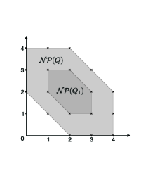
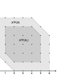
Figure 2. Relevant Newton polygons.

2.3.7. Common zeros of $Q$ and $R$ outside $\mathbb{R}_{+}^{2}$

By Lemma 2.8 the quadratic polynomials $\xi_{1},\xi_{2}$ and $\xi_{3}$ have two common zeros. Denote them by $(f_{1},g_{1})$ and $(f_{2},g_{2})$. Evidently, they are not real (e.g. since $\xi_{3}$ is strictly positive on $\mathbb{R}^{2}$).

Lemma 2.21.

$(f_{1},g_{1})$ and $(f_{2},g_{2})$ are solutions of the system $Q=R=0$ of multiplicity at least 6 each.

Proof.

Since $(f_{1},g_{1})$ and $(f_{2},g_{2})$ are conjugate and the system $Q=R=0$ is real, it suffices to consider one of these points, say $(f_{1},g_{1})$.

From (2.12) one can immediately see that $Q(f_{1},g_{1})=0$. Moreover, differentiating $Q_{1}$, one can see that $\frac{\partial Q_{1}}{\partial f}(f_{1},g_{1})=\frac{\partial Q_{1}}{\partial g}(f_{1},g_{1})=0$, so $(f_{1},g_{1})$ a critical point of $Q$.

Recall that $R=dQ\wedge\left(g\xi_{2}(-\frac{\xi_{3}}{1+\alpha}+f\xi_{3}^{\prime})df+f\xi_{3}(\frac{\xi_{2}}{1+\alpha}-g\xi_{2}^{\prime})dg\right)$, i.e. $R$ is the product of two polynomial forms each having a simple zero at $(f_{1},g_{1})$. Therefore this point is necessarily a critical point of $R$ as well.

Moreover, the 1-jet of $\eta_{2}$ at $(f_{1},g_{1})$ equals

$$j^{1}\eta_{2}=f_{1}g_{1}\xi_{2}^{\prime}(g_{1})\xi_{3}^{\prime}(f_{1})\left[\vphantom{\|\bigotimes}(g-g_{1})df-(f-f_{1})dg\right],$$

i.e. is proportional to the Euler form. Therefore, the quadratic part of $R$ at $(f_{1},g_{1})$ is proportional to the exterior product of the differential of the quadratic part of $Q$ at $(f_{1},g_{1})$ and the Euler form, so is proportional to the quadratic form of $Q$ at $(f_{1},g_{1})$. Thus a suitable linear combination of $R$ and $Q$ has both linear and quadratic part zero at $(f_{1},g_{1})$, which implies that the multiplicity of $(f_{1},g_{1})$ as a solution of the system $Q=R=0$ is at least 6. ∎

Lemma 2.22.

At least six real solutions of $Q=R=0$ lie outside $\mathbb{R}_{+}^{2}$.

Proof.

There are exactly four points where the form $\eta_{2}$ vanishes, exactly one in each real quadrant. These points are evidently solutions of the system $Q=R=0$. Consider a connected component of the curve $\{Q=0\}$ containing such a point. It is a compact oval not intersecting the coordinate axes. The polynomial $R$ vanishes at least once on this component, namely at this point. Therefore, $R$ should have at least one another zero on this oval (counting with multiplicities), also necessarily lying in the same quadrant. ∎

2.3.8. Final count

The number $N$ of points in the intersection $\gamma_{1}\cap\gamma_{2}\cap\mathbb{R}_{+}^{2}$ is less or equal $2+0+28-18=12$, where $2$ is the number of unbounded components of $\gamma_{1}$ in $\mathbb{R}_{+}^{2}$; $0$ is the number of unbounded components of $\{Q=0\}$; $28$ is the Kushnirenko-Bernstein upper bound for the number of complex solution of $R=Q=0$ in $(\mathbb{C}^{*})^{2}$ and $18$ is the number of solutions of $R=Q=0$ outside $\mathbb{R}_{+}^{2}$ counted with multiplicities. Therefore, Proposition 2.9 and Theorem 1.5.b are finally proved. ∎

2.3.9. Comments on Theorem 1.5

1. Computer experiments indicate that, except for the two solutions of the system $\xi_{1}=\xi_{2}=\xi_{3}=0$, all the remaining 16 solutions of the system $R=Q=0$ can be real. However, not all of them lie in the positive quadrant: typically the system $R=Q=0$ has 4 solutions in each real open quadrant. This implies that, provided that this statement about the root configuration could be rigorously proved, the best estimate obtainable by the above method would be $6$, very close to Maxwell’s conjectural bound $4$.

2. An even more important observation is that there are typically only two points of intersection of $\gamma_{2}$ and $\Gamma=\{Q=0\}$ lying in $\mathbb{R}_{+}^{2}$. In other words, the first application of the Rolle-Khovanskii lemma numerically seems to be exact: a rigorous proof that there are just two points in $\gamma_{1}\cap\Gamma\cap\mathbb{R}_{+}^{2}$ would imply the original Maxwell conjecture.

In fact, it is enough to prove a seemingly simpler statement that the number of intersections of $\Gamma$ and $\gamma_{1}=\{f^{1/(\alpha+1)}\rho_{1}-\rho=0\}$ lying in $\mathbb{R}_{+}^{2}$ is at most two. This seems to be easier since the equation defining $\gamma_{1}$, being quadratic polynomial in $g$, can be solved explicitly. The resulting two solutions $g=g_{1,2}(f)$ parameterize $\gamma_{1}$, and the problem reduces to the question about the number of positive zeros of a univariate algebraic function $Q(f,g_{1}(f))$.

3. The fact that the polynomial $R$ can be reduced to a smaller polynomial $\tilde{R}$ by subtraction of a multiple of $Q$ is a manifestation of a general yet unexplained phenomenon: tuples of polynomials resulting from several consecutive applications of the Rolle-Khovanskii theorem are very far from generic, and in every specific case one can usually make a reduction similar to the reduction of $R$ to $\tilde{R}$ above.

2.4. Proof of Theorem 1.6.a

From now on we will always assume that all our charges are positive (the case of all negative charges follows by a global sign change).

2.4.1. $1$-dimensional case

As a warm-up exercise we will prove Theorem 1.6.b in the simplest case of $x$-axis.

The idea of the proof is to use the limit function

(2.13) $$V_{\infty}(x)=\min_{i=1,\ldots,l}((x-x_{i})^{2}+y_{i}^{2})=\lim_{\alpha\to\infty}V_{\alpha}^{-1/\alpha}(x),$$

where $(x_{i},y_{i}),\;i=1,\ldots,l$ are the coordinates of the $i$-th charge. (We assume for simplicity that all $y_{i}\neq 0$. The general case follows by taking the limit.) The function $V_{\infty}(x)$ has at most $l-1$ points of non-smoothness. Denote these points by $\gamma_{j}$’s.

Lemma 2.23.

Convergence $V_{\infty}(x)=\lim_{\alpha\to\infty}V_{\alpha}^{-1/\alpha}(x)$ is valid in the $C^{2}$-class on any closed interval free from $\gamma_{j}$’s.

Proof.

We assume that on such an interval $\rho_{1}<(1-\eta)\rho_{i}$, $i\geq 2$, $\eta>0$. (Here $\rho_{i}=(x-x_{i})^{2}+y_{i}^{2}$.) Therefore, $V_{\infty}(x)=\rho_{1}$ on this interval. The first derivative of $V_{\infty}(x)$ equals

$$(V_{\alpha}^{-1/\alpha}(x))^{\prime}=-\frac{1}{\alpha}V_{\alpha}^{-1/\alpha-1}(x)\left(-\alpha\sum_{i=1}^{l}2\zeta_{i}\rho_{i}^{-\alpha-1}(x-x_{i})\right)=$$

$$=2\left[\zeta_{1}(x-x_{1})+\sum_{i=2}^{l}\zeta_{i}(\rho_{i}/\rho_{1})^{-\alpha-1}(x-x_{i})\right]\left(\rho_{1}^{\alpha}V_{\alpha}(x)\right)^{-2/\alpha-1}=$$

$$=2[\zeta_{1}(x-x_{1})+o(1)](\zeta_{1}+o(1))^{-2/\alpha-1}=2(x-x_{1})+o(1)=V_{\infty}^{\prime}(x)+o(1),$$

where $\lim_{\alpha\to\infty}o(1)=0$.

Computations with the second derivative are similar, but more cumbersome. ∎

Corollary 2.24.

For $\alpha$ sufficiently large any closed interval free from $\gamma_{j}$’s contains at most one critical point of $V_{\alpha}(x)$.

Proof.

Indeed, for any sufficiently large $\alpha$ the second derivative $(V_{\alpha}^{-1/\alpha}(x))^{\prime\prime}$, being close to $V_{\infty}^{\prime\prime}=2$, is positive on this interval. Therefore, $V_{\alpha}^{-1/\alpha}(x)$ is convex and can have at most one critical point on this interval. But the critical points of $V_{\alpha}^{-1/\alpha}(x)$ are the same as the critical points of $V_{\alpha}(x)$. ∎

Lemma 2.25.

For any sufficiently large $\alpha$ a closed interval containing some $\gamma_{j}$ and free from $x_{i}$’s contains at most one critical point of $V_{\alpha}(x)$.

Proof.

Note that such an interval contains exactly one $\gamma_{j}$ since $\gamma_{j}$’s are separated by $x_{i}$’s. The required result follows from the fact that $V_{\alpha}(x)$ is necessarily convex on any such interval. Indeed,

$$(V_{\alpha}(x))^{\prime\prime}=\alpha(\alpha+1)\sum_{i=1}^{l}\zeta_{i}\rho_{i}^{-\alpha-2}\left(4(x-x_{i})^{2}-\frac{2\rho_{i}}{\alpha+1}\right).$$

Since $x-x_{i}\not=0$ on the interval under consideration, then $\frac{2\rho_{i}}{\alpha+1}$ is necessarily smaller than $4(x-x_{i})^{2}$ for $\alpha$ large enough. Thus, $(V_{\alpha}(x))^{\prime\prime}$ is positive (recall that $\zeta_{i}>0$) and $V_{\alpha}(x)$ itself is convex. ∎

2.4.2. Multidimensional case

We start with the discussion of the critical points of the limiting function $V_{\infty}(\bar{x})$.

2.4.3. Critical points of $V_{\infty}(\bar{x})$

The function $V_{\infty}(\bar{x})$ is a piecewise smooth continuous semialgebraic function. Here are the definitions of critical points of such functions and their Morse indices adapted to our situation.

Definition 2.26.

A point $\bar{x}_{0}$ is a critical point of $V_{\infty}(\bar{x})$ if for any sufficiently small ball $B$ centered at $\bar{x}_{0}$ its subset $B_{-}=\{V_{\infty}(\bar{x})<V_{\infty}(\bar{x}_{0})\}\subseteq B$ is either empty or noncontractible.

The critical point $\bar{x}_{0}$ is called nondegenerate if $B_{-}$ is either empty or homologically equivalent to a sphere. In this case the Morse index of $\bar{x}_{0}$ is defined as the dimension of this sphere plus $1$. (By default, $\dim(\emptyset)=-1$.)

Lemma 2.27.

Every effective Voronoi cell of the Voronoi diagram of a generic configuration of positive charges contains a unique critical point of $V_{\infty}(\bar{x})$. Its index equals the dimension of the Voronoi cell.

Proof.

Indeed, take any effective Voronoi cell $S$. As above let $\mathcal{NS}(S)$ denote the set of all nearest sites of $S$. By definition, $S$ intersects the convex hull of $\mathcal{NS}(S)$. Denote this (unique) intersection point by $p(S)$. We claim that $p(S)$ is the unique critical point of $V_{\infty}(\bar{x})$ located on $S$. Indeed, the function $V_{\infty}(\bar{x})$ restricted to $\mathcal{NS}(S)$ has a local maximum at $p(S)$ since any sufficiently small move within $\mathcal{NS}(S)$ brings us closer to one of the nearest sites. (Here we implicitly use the genericity assumptions on the configuration, i.e. that there are exactly $k+1$ nearest sites for any Voronoi cell of codimension $k$ and that $S$ intersects the interior of the closure of $\mathcal{NS}(S)$.) On the other hand, the restriction of $V_{\infty}(\bar{x})$ to $S$ itself has the global minimum on $S$ for similar reasons. ∎

         

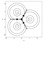
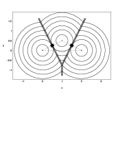
Figure 3. Effective and ineffective $0$-dimensional Voronoi cell of $V_{\infty}(\bar{x})$.

Remark. Figure 3 illustrates the above Lemma 2.27. The left picture shows the function $V_{\infty}(\bar{x})=\min(\rho_{1},\rho_{2},\rho_{3})$ where the three points are located at $(1,0),\;$ $(\pm\frac{\sqrt{3}}{2},-\frac{1}{2}),\;$. It is related to the left picture on Figure 1 showing the corresponding potential $V_{\alpha}(\bar{x})$ for $\alpha=1$. In this case all the Voronoi cells of the Voronoi diagram are effective and one sees the local maximum inside the convex hull of these points. On the right picture the three points are located at $(0,0),\;(2,0),\;(1,\frac{1}{2})$. In this case the $0$-dimensional Voronoi cell and one of $1$-dimensional Voronoi cells are ineffective and there is no critical point at the $0$-dimensional Voronoi cell. This picture is similarly related to the right picture on Figure 1.

2.4.4. Proof continued

In order to settle the multidimensional case we generalize the previous proof using the following idea.

Main idea for zero-dimensional Voronoi cells: Near an effective zero-dimensional Voronoi cell of the Voronoi diagram the union of the region where $V_{\alpha}(\bar{x})$ is convex (and therefore has at most one critical point) and the region where $V_{\alpha}(\bar{x})$ is too $\mathcal{C}^{1}$-close to $V_{\infty}^{-\alpha}(\bar{x})$ to have any critical points asymptotically covers a complete neighborhood of the Voronoi cell. More exact, we compute asymptotics of the sizes of the above regions, and show that the first region shrinks slower than the second region grows.

The following expressions for the gradient and the Hessian form (i.e., the quadratic form defined by the matrix of the $2$-nd partial derivatives) of $V_{\alpha}(\bar{x})$ are crucial for further computations:

$$\nabla V_{\alpha}({\bar{x}}) = -\alpha\sum_{i=1}^{l}\zeta_{i}\rho_{i}^{-\alpha-1}(\bar{x})\nabla\rho_{i}(\bar{x}),$$

$$\operatorname{Hess}V_{\alpha}(\bar{x})\cdot\xi = \alpha(\alpha+1)\sum_{i=1}^{l}\zeta_{i}\rho_{i}^{-\alpha-2}(\bar{x})\left((\nabla\rho_{i}(\bar{x}),\xi)^{2}-\frac{2}{\alpha+1}\rho_{i}(\bar{x})\|\xi\|^{2})\right).$$

Here ${}^{\prime}\,\cdot\,^{\prime}$ denotes the evaluation of the quadratic form $\operatorname{Hess}V_{\alpha}(\bar{x})$ at $\xi$.

We start with the case of zero-dimensional Voronoi cells. The general case will be a treated as a direct product of the zero-dimensional case in the direction transversal to the Voronoi cell and the full-dimensional case along the Voronoi cell.

2.4.5. Zero-dimensional Voronoi cells of Voronoi diagram.

Let $S$ be a zero-dimensional Voronoi cell of a Voronoi diagram of a generic configuration. We can assume that $\rho_{1}(S)=...=\rho_{n+1}(S)<\rho_{i}(S)$ for $i>n+1$. Set

$$\phi(\bar{x})=\log\left(\frac{\max_{i=1,...,n+1}\rho_{i}(\bar{x})}{\min_{i=1,...,n+1}\rho_{i}(\bar{x})}\right).$$

Note that $\phi(\bar{x})$ is everywhere positive except at the origin, and is equivalent to the Euclidean distance to $S$ in a sufficiently small neighborhood of $S$.

Lemma 2.28.

There exists $\delta>0$ so small that in the $\delta$-neighborhood $\mathcal{U}$ of $S$ the following conditions hold:

1. There exists a number $\epsilon>0$ such that for any $\bar{x}\in\mathcal{U}$

   $$\min_{i=n+1,n+2,\ldots,l}\rho_{i}(\bar{x})>e^{2\epsilon}\min_{i=1,2,\ldots,n+1}\rho_{i}(\bar{x})>e^{\epsilon}\max_{i=1,\ldots,n+1}\rho_{i}(\bar{x}).$$

   In particular, $\phi(\bar{x})<\epsilon$ in $\mathcal{U}$.

2. The absolute value of all ratios $c_{k}(\bar{x})/c_{l}(\bar{x})$ in the unique linear dependence $\sum_{i=1}^{n+1}c_{i}(\bar{x})\nabla\rho_{i}(\bar{x})=0$ is bounded by some constant $\Upsilon>0$ (by the genericity of configuration none of $c_{k}(S)$’s vanishes on $S$ and, therefore, in some neighborhood of $S$ as well).

3. If the cell $S$ is not effective, then the closure of $\mathcal{U}$ can be separated from the convex hull of $\mathcal{NS}(S)$ by a hyperplane.

We prove that for $\alpha$ sufficiently large the domain $\mathcal{U}$ is the union of two subdomains $\mathcal{U}=U_{1}\cup U_{2}$ such that $V_{\alpha}(\bar{x})$ is convex in $U_{1}$, and $\nabla V_{\alpha}(\bar{x})\not=0$ in $U_{2}$.

In what follows we denote by $C_{k}$ and $\kappa_{k}$ positive constants independent of $\alpha$ but dependent on the configuration and the choice of $\mathcal{U}$.

Lemma 2.29.

There exists a constant $\kappa_{1}$ independent of $\alpha$ such that for $\alpha$ sufficiently large the function $V_{\alpha}(\bar{x})$ has no critical points in the domain defined by $\{\phi(\bar{x})>\frac{\kappa_{1}}{\alpha+1}\}\cap\mathcal{U}.$

Proof.

First, consider the case $l=n+1$.

The condition $\nabla V_{\alpha}(\bar{x})=0$ implies that

$$\frac{\zeta_{i}}{\zeta_{j}}\left(\frac{\rho_{i}}{\rho_{j}}\right)^{-\alpha-1}=\frac{c_{j}}{c_{j}}\leq\Upsilon,$$

and, taking the logarithm of the both sides, we arrive at $\phi(\bar{x})<\frac{\log\Upsilon+\log\max_{i,j}(c_{i}/c_{j})}{\alpha+1}$. Thus one can take $\kappa_{1}={\log\Upsilon+\log\max_{i,j}(c_{i}/c_{j})}$ in this case.

The case $l>n+1$ differs by exponentially small terms. Namely, suppose that $\rho_{1}(\bar{x})=\max\rho_{i}(\bar{x})$. Then

$$0=\rho_{1}^{\alpha+1}\nabla V_{\alpha}(\bar{x})=(\zeta_{1}\nabla\rho_{1}-\xi)+\sum_{i=2}^{n+1}\zeta_{i}\left(\frac{\rho_{i}}{\rho_{1}}\right)^{-\alpha-1}\nabla\rho_{i},$$

where $\xi=\sum_{i=n+2}^{l}\zeta_{i}(\rho_{i}/\rho_{1})^{-\alpha-1}\nabla\rho_{i}$. One can easily see that $\|\xi\|\leq C_{1}e^{-\epsilon(\alpha+1)}$. Therefore, since $\nabla\rho_{2}(x),...,\nabla\rho_{n+1}(x)$ are linearly independent in $\mathcal{U}$,

$$|\zeta_{i}(\rho_{i}/\rho_{1})^{-\alpha-1}-\zeta_{1}c_{i}/c_{1}|\leq C_{2}e^{-\epsilon(\alpha+1)}=o(1),$$

and we get the required estimate. ∎

Lemma 2.30.

There exists a constant $\kappa_{2}$ independent of $\alpha$ such that for all sufficiently large $\alpha$ the function $V_{\alpha}(\bar{x})$ is convex in the domain $\{\phi(\bar{x})<\frac{\log(\alpha+1)-\kappa_{2}}{\alpha+2}\}$.

Proof.

Again, start with the case $l=n+1$. The gradients $\nabla\rho_{i},i=1,...,n+1,$ span the whole $\mathbb{R}^{n}$. Thus, the quadratic form $\sum_{i=1}^{n+1}\zeta_{i}(\nabla\rho_{i}\cdot\xi)^{2}\geq C_{3}\|\xi\|^{2}>0$ is positive definite. Therefore, one gets

$$\frac{1}{\alpha(\alpha+1)}{\operatorname{Hess}V_{\alpha}(\bar{x})}\cdot\xi=\sum_{i=1}^{n+1}\zeta_{i}\rho_{i}^{-\alpha-2}(\nabla\rho_{i},\xi)^{2}-\frac{2}{\alpha+1}\sum_{i=1}^{n+1}\zeta_{i}\rho_{i}^{-\alpha-1}\|\xi\|^{2}\geq$$

$$\geq(\max_{i=1,...,n+1}\rho_{i})^{-\alpha-2}\left(\sum_{i=1}^{n+1}\zeta_{i}(\nabla\rho_{i},\xi)^{2}\right)-\frac{2(n+1)(\min_{i=1,...,n+1}\rho_{i})^{-\alpha-1}\max_{i=1,...,n+1}\zeta_{i}}{\alpha+1}\|\xi\|^{2}\geq$$

$$\geq(\min_{i=1,...,n+1}\rho_{i})^{-\alpha-2}\left(C_{3}\cdot(e^{\phi(\bar{x})})^{-\alpha-2}-\frac{C_{4}}{\alpha+1}\right)\|\xi\|^{2}.$$

The last form is positive definite if

(2.14) $$e^{-(\alpha+2)\phi(\bar{x})}>\frac{C_{5}}{\alpha+1}\text{ or, equivalently, }\phi(\bar{x})<\frac{\log(\alpha+1)-\kappa_{2}}{\alpha+2}.$$

The case $l>n+1$ differs by an exponentially small term, namely by the term

$$\left|\sum_{i=n+2}^{l}\zeta_{i}\rho_{i}^{-\alpha-2}\left[(\nabla\rho_{i},\xi)^{2}-\frac{2\rho_{i}}{\alpha+1}\|\xi\|^{2}\right]\right|\leq C_{6}(\min_{i=1,...,n+1}\rho_{i})^{-\alpha-2}e^{-\epsilon(\alpha+2)}\|\xi\|^{.}$$

Therefore, instead of (2.14) we get that $\operatorname{Hess}V$ is positive definite provided

$$e^{-(\alpha+2)\phi(\bar{x})}>\frac{C_{5}}{\alpha+1}+C_{6}e^{-\epsilon(\alpha+2)},$$

which gives the same estimate with a different constant. ∎

Lemma 2.31.

$V_{\alpha}(\bar{x})$ has at most one critical point in $\mathcal{U}$. If the cell under consideration is effective then the critical point exists and is a local minimum. If the cell under consideration is not effective then there is no critical point in $\mathcal{U}$.

Proof.

Indeed, in the above notation for sufficiently large $\alpha$ one has

$$\frac{\log(\alpha+1)-\kappa_{2}}{\alpha+2}>\frac{\kappa_{1}}{\alpha+1}.$$

Thus $\mathcal{U}$ is covered by two domains, $\{\phi(\bar{x})>\frac{\kappa_{1}}{\alpha+1}\}$ and $\{\phi(\bar{x})\leq\frac{\log(\alpha+1)-\kappa_{2}}{\alpha+2}\}$. By Lemma 2.29 $V_{\alpha}(\bar{x})$ has no critical points in the first domain. By Lemma 2.30 $V_{\alpha}(\bar{x})$ is convex and has at most one critical point in the second domain.

In the case when the considered $0$-dimensional Voronoi cell is effective $V_{\alpha}(\bar{x})$ actually has a local minimum located close to that Voronoi cell: the function $V_{\alpha}^{-1/\alpha}(\bar{x})$, being $\mathcal{C}^{0}$-close to $V_{\infty}$, has a local minimum inside $\mathcal{U}$.

The last statement is a particular case of the Lemma 2.35 below. ∎

Taken together, this proves that for $\alpha$ sufficiently large to each effective zero-dimensional Voronoi cells of a generic configuration of points corresponds exactly one minimum of $V_{\alpha}$.

2.4.6. Case of arbitrary codimension

Let $S$ be any Voronoi cell of codimension $k$ of the Voronoi diagram. We prove that for a generic configuration of positive charges and any compact $K\subset S$ lying inside $S$ there exists a sufficiently small neighborhood $\mathcal{U}_{K}$ independent of $\alpha$ containing at most one critical point of $V_{\alpha}(\bar{x})$. Moreover, this critical point exists if and only if the cell is effective, and its Morse index is equal to $n-k$.

Denote by $L$ the affine subspace spanned by $S$. Recall that the first genericity assumption means that there exist exactly $k+1$ charges $\zeta_{1},...,\zeta_{k+1}$ closest to $S$. Denote the affine subspace orthogonal to $L$ spanned by these charges by $M$.

Lemma 2.32.

$\dim M=k$.

Proof.

Indeed, a small shift of any point of $S$ in any direction orthogonal to $M$ produces a point with the same set of closest charges: distances to charges not in $\mathcal{NS}(S)$ will still remain bigger than the distances to the charges in $\mathcal{NS}(S)$, and the latter distances will remain equal. Therefore the shifted point still lies in $S$, so the dimension of $S$ is at least $\operatorname{codim}M$, i.e., $\dim M\geq k$. The opposite inequality is evident since $\mathcal{NS}(S)$ contains $k+1$ points. ∎

If the Voronoi cell $S$ intersects the convex hull of $\mathcal{NS}(S)$ then the second genericity assumption means that any $k$ of charges in $\mathcal{NS}(S)$ do not lie on a hyperplane in $M$ passing through the point $L\cap M$.

Choosing an appropriate coordinate system we may assume that $L$ and $M$ intersect at the origin, i.e. are orthogonal complements of each other. Denote by $\bar{x}_{L}$ and $\bar{x}_{M}$ orthogonal projections of a vector $\bar{x}$ to linear subspaces $L$ and $M$ resp. i.e. $\bar{x}=\bar{x}_{M}+\bar{x}_{L}$. Finally, denote the distances from $\bar{x}$ to the charges $\zeta_{1},...,\zeta_{k+1}$ in $\mathcal{NS}(S)$ by $\rho_{1},...,\rho_{k+1}$ resp.

Let $K$ be a compact subset of $S$.

Lemma 2.33.

There exists $\delta>0$ so small that in the $\delta$-neighborhood $\mathcal{U}_{K}\subset\mathbb{R}^{n}$ of $K$ the following conditions hold:

1. $\exists\,0<\epsilon\ll 1$ such that for any $\bar{x}\in\mathcal{U}_{K}$ one has

   $$\min_{i=k+2,\ldots,l}\rho_{i}>e^{2\epsilon}\min_{i=1,\ldots,k+1}\rho_{i}>e^{\epsilon}\max_{i=1,\ldots,k+1}\rho_{i}.$$

   This is possible since $K$ is a compact subset of an open Voronoi cell $S$, and is therefore located on some positive distance from other Voronoi cells.

2. The absolute value of all ratios $c_{k}(\bar{x})/c_{l}(\bar{x})$ in the unique linear dependence $\sum_{j=1}^{k+1}c_{k}(\bar{x})\nabla_{M}\rho_{j}=0$ is bounded from above by some constant $\Upsilon$, where $\nabla_{M}\rho_{j}$ denotes the orthogonal projection of the gradient $\nabla\rho_{j}$ to $M$. Note that the tuple of $c_{k}(\bar{x})$ is, up to proportionality, constant on $S$, and none of $c_{k}$ vanishes due to the second genericity assumption.

3. If the cell $S$ is not effective, then the closure of $\mathcal{U}$ can be separated from the convex hull of $\mathcal{NS}(S)$ by a hyperplane.

As before, introduce the function

$$\phi_{M}(\bar{x})=\log\left(\frac{\max_{i=1,\ldots,k+1}\rho_{i}}{\min_{i=1,\ldots,k+1}\rho_{i}}\right).$$

This function is equivalent to $\|\bar{x}_{M}\|$ near the origin:

(2.15) $$C_{M}^{-1}\phi_{m}(\bar{x})\leq\|\bar{x}_{M}\|\leq C_{M}\phi_{M}(\bar{x})$$

for some $C_{M}>0$ and all $x\in\mathcal{U}$.

Lemma 2.34.

a) For a certain positive $\kappa_{3}$ the function $V_{\alpha}(\bar{x})$ has no critical points in the domain given by $\mathcal{U}_{K}\cap\{\|\bar{x}_{L}\|>\kappa_{3}\cdot e^{-\epsilon(\alpha+1)}\}$.

b) For a certain positive $\kappa_{4}$ the function $V_{\alpha}(\bar{x})$ has no critical points in the domain given by $\mathcal{U}_{K}\cap\{\phi_{M}(\bar{x})>\frac{\kappa_{4}}{\alpha+1}\}$.

Proof.

a) The idea is that outside $L$ the gradients of $\rho_{i}$’s, $i=1,...,k+1$, are all directed away from $L$. The contribution of the remaining $\rho_{i}$’s, being exponentially small, is negligible outside an exponentially small neighborhood.

We calculate the directional derivative of $V_{\alpha}(\bar{x})$ in the direction $\bar{x}_{L}$ at a point $\bar{x}\in\mathcal{U}_{K}$.

$$-\frac{1}{\alpha}\frac{\partial V_{\alpha}(\bar{x})}{\partial\bar{x}_{L}}(\bar{x})=\sum_{i=1}^{k+1}\zeta_{i}\rho_{i}^{-\alpha-1}\frac{\partial\rho_{i}}{\partial\bar{x}_{L}}(\bar{x})+\sum_{i=k+2}^{l}\zeta_{i}\rho_{i}^{-\alpha-1}\frac{\partial\rho_{i}}{\partial\bar{x}_{L}}(\bar{x}).$$

Since $\frac{\partial\rho_{i}}{\partial\bar{x}_{L}}(\bar{x})=2\|\bar{x}_{L}\|^{2}$ for $i=1,...,k+1$, we conclude that the absolute value of the first term is at least $C_{9}(\max_{i=1,\ldots,k+1}\rho_{i})^{-\alpha-1}\|\bar{x}_{L}\|^{2}$. The absolute value of the second term is at most

$$C_{10}(\min_{i=k+2,\ldots,l}\rho_{i})^{-\alpha-1}\|\bar{x}_{L}\|<C_{10}(\max_{i=1,\ldots,k+1}\rho_{i})^{-\alpha-1}e^{-\epsilon(\alpha+1)}\|\bar{x}_{L}\|,$$

and the estimate follows.

b) We essentially repeat the computations of Lemma 2.29.

$$-\frac{1}{\alpha}\nabla_{M}V_{\alpha}(\bar{x})=\sum_{i=1}^{k+1}\zeta_{i}\rho_{i}^{-\alpha-1}\nabla_{M}\rho_{i}(\bar{x})+\sum_{j=k+2}^{l}\zeta_{i}\rho_{j}^{-\alpha-1}\nabla_{M}\rho_{j}(\bar{x})=$$

$$=(\max_{j=1,\ldots,k+1}\rho_{j})^{-\alpha-1}\left[\sum_{i=1}^{k+1}\zeta_{i}\left(\frac{\rho_{i}}{\max_{j=1,\ldots,k+1}\rho_{j}}\right)^{-\alpha-1}\nabla_{M}\rho_{i}(\bar{x})+O(e^{-\epsilon(\alpha+1)})\right].$$

So $\nabla_{M}V_{\alpha}(\bar{x})=0$ implies, as in Lemma 2.29, that the functions $\left(\frac{\rho_{i}}{\max_{j=1,\ldots,k+1}\rho_{j}}\right)^{-\alpha-1}$ are bounded, which gives:  $\phi_{M}(\bar{x})<\frac{\kappa_{4}}{\alpha+1}$.

∎

Lemma 2.35.

If the cell $S$ is not effective then for $\alpha$ large enough the function $V_{\alpha}(\bar{x})$ has no critical points in $\mathcal{U}_{K}$.

Proof.

Let $\mathfrak{n}$ be a direction normal to the hyperplane separating $\mathcal{U}_{K}$ from the convex hull of $\mathcal{NS}(S)$. Then $\zeta_{i}(\nabla\rho_{i},\mathfrak{n})$ are all of the same sign in $\mathcal{U}$ (say, negative), and of absolute value greater than some positive constant $C_{7}$. Therefore

$$|(\nabla V_{\alpha},\mathfrak{n})| = \alpha|\sum_{i=1}^{l}\zeta_{i}\rho_{i}^{-\alpha-1}(\nabla\rho_{i},\mathfrak{n})|\geq$$

$$\geq \alpha\left[C_{7}(k+1)(\max_{i\leq k+1}\rho_{i})^{-\alpha-1}-C_{8}(\min_{i>k+1}\rho_{i})^{-\alpha-1}\right]\geq$$

$$\geq \alpha(\max_{i=1,...,k+1}\rho_{i})^{-\alpha-1}\left((k+1)C_{7}-C_{8}e^{-\epsilon(\alpha+1)}\right)>0$$

for $\alpha$ large enough. ∎

From now on we suppose that $K$ and the convex hull of $\mathcal{NS}(S)$ intersect at the origin, and consider the domain

(2.16) $$\mathcal{U}_{\alpha}=\left\{\bar{x}_{L}<\kappa_{3}\cdot e^{-\epsilon(\alpha+1)},\|\bar{x}_{M}\|<\frac{C_{M}\kappa_{4}}{\alpha+1}\right\}\subset\mathcal{U}_{K}.$$

Union of this domain and the domain described in Lemma 2.34 covers $\mathcal{U}$ by (2.15). Moreover, $\phi_{M}(\bar{x})\leq\frac{C_{M}^{2}\kappa_{4}}{\alpha+1}$ in $\mathcal{U}$.

Our next goal is to study the quadratic form $\operatorname{Hess}V_{\alpha}(\bar{x})$ in the domain $\mathcal{U}_{\alpha}$.

Lemma 2.36.

Let $V_{k,\alpha}(\bar{x})=\sum_{i=1}^{k+1}\zeta_{i}\rho_{i}^{-\alpha}$. The following holds

a)$\operatorname{Hess}V_{\alpha}(\bar{x})-\operatorname{Hess}V_{k,\alpha}(\bar{x})=(\max_{i=1,\ldots,k+1}\rho_{i})^{-\alpha-2}O(e^{-\epsilon\alpha})$ for $\bar{x}\in\mathcal{U}_{\alpha}$ and $\alpha\to\infty$.

b) There exist two quadratic forms $A(x)$ and $B(x)$ on $M$ and $L$ resp. such that $\operatorname{Hess}V_{k,\alpha}(\bar{x})-A(\bar{x})\oplus B(\bar{x})=(\max_{i=1,\ldots,k+1}\rho_{j})^{-\alpha-2}O(e^{-\epsilon\alpha})$.

There exist some positive constants $\kappa_{5},\kappa_{6}$ such that the form $A$ is positive definite and bounded from below by a $\kappa_{5}\cdot\alpha^{2}(\max_{i=1,\ldots,k+1}\rho_{i})^{-\alpha-2}$, and the form $B$ is negative definite and bounded from above by $-\kappa_{6}\cdot\alpha(\max_{i=1,\ldots,k+1}\rho_{i})^{-\alpha-2}$.

Proof.

a) We have to estimate from above the contribution of the distant charges.

$$|\operatorname{Hess}V_{\alpha}(\bar{x})\cdot\xi-\operatorname{Hess}V_{k,\alpha}(\bar{x})\cdot\xi|\leq\alpha(\alpha+1)\sum_{i=k+2}^{l}\zeta_{i}\rho_{i}^{-\alpha-2}((\nabla\rho_{i},\xi)^{2}-\frac{2}{\alpha+1}\rho_{i}\|\xi\|^{2})\leq$$

$$\leq C\dot{(}\max_{i=1,\ldots,k+1}\rho_{i})^{-\alpha-2}e^{-\epsilon(\alpha+2)}\|\xi\|^{2}.$$

b) For $i=1,...,k+1$ the charges $\zeta_{i}$ are in $M$. Therefore we have

$$(\nabla\rho_{i}(\bar{x}),\xi)^{2}=(\nabla_{M}\rho_{i}(\bar{x}),\xi_{M})^{2}+2(\nabla_{M}\rho_{i}(\bar{x}),\xi_{M})(\nabla_{L}\rho_{i}(\bar{x}),\xi_{L})+(\nabla_{L}\rho_{i}(\bar{x}),\xi_{L})^{2}=$$

$$=(\nabla_{M}\rho_{i}(\bar{x}),\xi_{M})^{2}+O(e^{-\epsilon\alpha})\|\xi\|^{2}.$$

Here we used $\nabla_{L}\rho_{j}(\bar{x})=2\bar{x}_{L}$, and $\|\bar{x}_{L}\|\leq\kappa_{3}e^{-\epsilon\alpha}$ in $\mathcal{U}_{\alpha}$.

Therefore,

$$\operatorname{Hess}V_{k,\alpha}(\bar{x})\cdot\xi=\alpha(\alpha+1)\sum_{i=1}^{k+1}\zeta_{i}\rho_{i}^{-\alpha-2}\left[(\nabla\rho_{i},\xi)^{2}-\frac{2}{\alpha+1}\rho_{i}\|\xi\|^{2}\right]=$$

$$=\alpha(\alpha+1)\sum_{i=1}^{k+1}\zeta_{i}\rho_{i}^{-\alpha-2}(\nabla_{M}\rho_{i},\xi_{M})^{2}-2\alpha\sum_{i=1}^{k+1}\zeta_{i}\rho_{i}^{-\alpha-1}\|\xi\|^{2}+O(e^{-\epsilon\alpha})\sum_{i=1}^{k+1}\rho_{i}^{-\alpha-2}\|\xi\|^{2}.$$

Due to linear independence of $\nabla_{M}\rho_{j}$’s in $\mathcal{U}_{\alpha}$ we get, exactly as in Lemma 2.30,

$$\sum_{i=1}^{l}\zeta_{i}(\nabla_{M}\rho_{i},\xi_{M})^{2}>C_{9}\|\xi_{M}\|^{2}$$

for some $C_{9}>0$. Therefore, one can estimate the first term from below as

$$\alpha(\alpha+1)\sum_{i=1}^{k+1}\zeta_{i}\rho_{i}^{-\alpha-2}(\nabla\rho_{j},\xi_{M})^{2}\geq\alpha(\alpha+1)C_{9}(\max_{i=1,\ldots,k+1}\rho_{i})^{-\alpha-2}\|\xi_{M}\|^{2}.$$

The second term can be estimated using

$$(\min\zeta_{i})(\max_{j=1,\ldots,k+1}\rho_{j})^{-\alpha-1}\leq\frac{1}{k+1}\sum_{j=1,\ldots,k+1}\zeta_{i}\rho_{j}^{-\alpha-1}\leq(\max\zeta_{i})(\max_{j=1,\ldots,k+1}\rho_{j})^{-\alpha-1}e^{(\alpha+1)\phi_{M}(\bar{x})}.$$

The expression $e^{(\alpha+1)\phi_{M}(\bar{x})}$ is bounded in $\mathcal{U}_{\alpha}$ by a constant $e^{C_{M}^{2}\kappa_{4}}$ independent of $\alpha$. Therefore the restriction of $\operatorname{Hess}V_{k,\alpha}(\bar{x})\cdot\xi$ to $M$ has the lower bound:

$$\alpha(\alpha+1)(\max_{i=1,\ldots,k+1}\rho_{i})^{-\alpha-2}\left(C_{9}-\frac{2(k+1)e^{C_{M}^{2}\kappa_{4}}\max_{i,\mathcal{U}}\zeta_{i}\rho_{i}}{\alpha+1}-O(e^{-\epsilon\alpha})\right)\|\xi_{M}\|^{2}.$$

On the other hand, the restriction of $\operatorname{Hess}V_{k,\alpha}(\bar{x})\cdot\xi$ to $L$ is negative definite and has the upper bound:

$$-2\alpha(k+1)\min\zeta_{i}(\max_{i=1,\ldots,k+1}\rho_{i})^{-\alpha-1}\|\xi_{L}\|^{2}\left(1-O(e^{-\epsilon\alpha})\right).$$

∎

Corollary 2.37.

For large enough $\alpha$ and any $\bar{x}\in\mathcal{U}_{\alpha}$ the signature of the quadratic form $\operatorname{Hess}V_{\alpha}(\bar{x})$ is $(k,n-k)$.

Lemma 2.38.

For sufficiently large $\alpha$ there is at most one critical point of $V_{\alpha}(\bar{x})$ in $\mathcal{U}_{K}$, and its Morse index is equal to $n-k$.

Proof.

As was proved in Lemma 2.34, there are no critical points of $V_{\alpha}$ in $\mathcal{U}_{K}\setminus\mathcal{U}_{\alpha}$ for $\alpha$ large enough. So it is enough to prove that the mapping $dV_{\alpha}$ is one-to-one in $\mathcal{U}_{\alpha}$.

Take any segment $I=\{a_{t}=a+t\xi,0\leq t\leq 1\}\subset\mathcal{U}_{\alpha}$. Let $\pi(t)$ be the projection of the point $dV_{\alpha}(a_{t})$ on the direction $\bar{\xi}=\xi_{M}-\xi_{L}$ (where $\xi=\xi_{m}+\xi_{L}$). We claim that $\pi(t)$ is a monotonous function of $t$, and, therefore, its values at $a_{0}$ and $a_{1}$ cannot coincide. Indeed, using Lemma 2.36 one can estimate $\pi^{\prime}(t)$ from below as

$$\pi^{\prime}(t)=\left(\bar{\xi},\frac{\partial}{\partial t}dV_{\alpha}(a_{t})\right)=\operatorname{Hess}V_{\alpha}(\bar{\xi},\xi)\geq$$

$$\geq(\max_{i=1,\ldots,k+1}\rho_{i})^{-\alpha-2}\left[\kappa_{5}\cdot\alpha^{2}\|\xi_{M}\|^{2}+\kappa_{6}\cdot\alpha\|\xi_{L}\|^{2}+O(e^{-\epsilon\alpha})\|\xi\|^{2}\vphantom{\frac{\mathbb{R}^{\mathbb{R}}_{\mathbb{R}}}{2}}\right]>0$$

for $\alpha$ sufficiently large.

This, by convexity of $\mathcal{U}_{\alpha}$, immediately implies the claim of the Lemma: assuming that there are two critical points and joining them by a segment we get a contradiction.∎

We proved in Lemma 2.35 that non-effective cells do not create critical points of $V_{\alpha}$ for $\alpha$ large enough. To finish the proof of the one-to-one correspondence between effective cells and critical points of $V_{\alpha}$ we have to show that if $K$ contains a critical point of the function $V_{\infty}$ then $\mathcal{U}_{K}$ does contain a critical point of $V_{\alpha}$.

Lemma 2.39.

Assume that $K$ contains a critical point of $V_{\infty}$. Then $\mathcal{U}_{K}$ contains a critical point of $V_{\alpha}$ for $\alpha$ sufficiently large.

The idea of the proof is that the smooth function $V_{\alpha}^{-\frac{1}{\alpha}}$ is arbitrarily $\mathcal{C}^{0}$-close to $V_{\infty}$ for large $\alpha$. The topology of the sets $X_{c}=\{V_{\infty}\leq c\}\cap{\mathcal{U}_{K}}$ changes as $c$ passes the critical value implying the change of the topology of the sets $Y_{c}=\{V_{\alpha}^{-\frac{1}{\alpha}}\leq c\}\cap{\mathcal{U}_{K}}$ for sufficiently large $\alpha$ which in its turn implies presence of the critical points of $V_{\alpha}^{-\frac{1}{\alpha}}$, the latter coinciding with the critical points of $V_{\alpha}$.

Let $c_{0}$ be the critical value of $V_{\infty}$ at the point $c\in K$, and let $c_{1}$, $c_{2}$ be some regular values, $\min_{\mathcal{U}_{K}}V_{\infty}<c_{1}<c_{0}<c_{2}<\max_{\mathcal{U}_{K}}V_{\infty}$. We assume that $c_{1},c_{2}$ are so close to $c_{0}$ that the interval $[c_{1},c_{2}]$ contains no critical values of $V_{\infty}$ restricted to the boundary of $\mathcal{U}_{K}$.

Let $\delta\ll(c_{0}-c_{1})/2$. For $\alpha$ large enough the function $V_{\alpha}^{-\frac{1}{\alpha}}$ is at least $\delta/2$-close to $V_{\infty}$. Thus, we have

$$X_{c_{1}}\subset Y_{c_{1}+\delta/2}\subset X_{c_{1}+\delta}\subset Y_{c_{1}+\frac{3}{2}\delta}.$$

These inclusions induce homomorphisms in homology groups:

(2.17) $$H_{*}(X_{c_{1}})\to H_{*}(Y_{c_{1}+\delta/2})\to H_{*}(X_{c_{1}+\delta})\to H_{*}(Y_{c_{1}+\frac{3}{2}\delta}).$$

The composition of the first two homomorphisms is a homomorphism induced by the inclusion $X_{c_{1}}\subset X_{c_{1}+\delta}$, which is an isomorphism. Therefore the middle homomorphism in (2.17) is surjective.

Similarly, the composition of the last two homomorphisms is a homomorphism induced by the inclusion $Y_{c_{1}+\delta/2}\subset Y_{c_{1}+\frac{3}{2}\delta}$, which, assuming that $V_{\alpha}^{-\frac{1}{\alpha}}$ has no critical points, is an isomorphism as well. Therefore the middle homomorphism in (2.17) is injective.

Summing up, we conclude that the middle homomorphism is an isomorphism, and $Y_{c_{1}}$ is homologically equivalent to $X_{c_{1}}$.

Similarly, $Y_{c_{2}}$ is homologically equivalent to $X_{c_{2}}$. But the sets $X_{c_{1}}$ and $X_{c_{2}}$ are not homologically equivalent: the first is homologically equivalent to a sphere, and the second is contractible. Therefore $Y_{c_{1}}$ and $Y_{c_{2}}$ are also homologically different implying that $V_{\alpha}^{-\frac{1}{\alpha}}$ should have a critical point in $\mathcal{U}_{K}$.

2.4.7. Completing the proof of Theorem 1.6.a

Since $V_{\alpha}$ has no critical points outside the convex hull of the charges, it is enough to consider instead of $\mathbb{R}^{n}$ an open ball $B$ containing all charges.

It is easy to see that one can cover $B$ by neighborhoods $\mathcal{U}_{k}$ as in Lemma 2.28 and 2.33. Indeed, start from zero-dimensional Voronoi cells $S_{i}$, and choose their neighborhoods $\mathcal{U}_{i}$ according to Lemma 2.28. Then choose compacts $K^{1}_{i}$ in one dimensional Voronoi cells in such a way that their union with these neighborhoods covers the intersection of the union of all one-dimensional Voronoi cells with $B$. Choose neighborhoods $\mathcal{U}_{K^{1}_{i}}$ of these compacts according to Lemma 2.33. Then choose compact subsets $K^{2}_{i}$ of two-dimensional Voronoi cells in such a way that $(\cup K^{2}_{i})\cup(\cup\mathcal{U}_{K^{1}_{i}})$ covers the intersection of the union of all two-dimensional Voronoi cells with $B$, and so on. At the end the union of all selected neighborhoods will cover $B$.

Each of the neighborhoods corresponding to effective Voronoi cells will contain one critical point of $V_{\alpha}$, and its Morse index will be equal to the dimension of the Voronoi cell. The neighborhoods of non-effective Voronoi cells will not contain critical points of $V_{\alpha}$.

2.5. Proof of Theorem 1.6.b

We are looking for the critical points of the function $\tilde{V}_{\alpha}$ defined in a linear space $N$

$$\tilde{V}_{\alpha}=\sum\zeta_{i}\tilde{\rho}_{i}^{-\alpha},\qquad\text{where}\quad\tilde{\rho}_{i}=\text{dist}^{2}(\bar{x},\tilde{c}_{i})+y_{i}^{2},$$

where $\tilde{c}_{i}$ are now orthogonal projections on $N$ of the positions $c_{i}$ of the charges $\zeta_{j}$. The claim is that the critical points of $\tilde{V}_{\alpha}$ are in one-to-one correspondence with the effective with respect to $N$ cells of the Voronoi diagram of $\{\zeta_{j}\}$.

We can characterize the partition of $N$ by intersections with the cells of the Voronoi diagram only in terms of $\tilde{\rho}_{i}$. Namely, a generalized Voronoi diagram in $N$ is defined as the classical Voronoi diagram in $1.1, with $\rho_{i}$ replaced by $\tilde{\rho}_{i}$: a cell $S$ of a generalized Voronoi diagram is the set of all points $\bar{x}\in N$ with the same set $\mathcal{NS}(S)=\{i|\forall k\quad\tilde{\rho}_{i}(\bar{x})\leq\tilde{\rho}_{k}(\bar{x})\}$. One can immediately see that thus defined generalized Voronoi diagram coincides with the intersection of the original Voronoi diagram with $N$.

It turns out that using this notation one can get the proof of Theorem 1.6.b from that of Theorem 1.6.a by a simple replacement of $\mathbb{R}^{n}$ by $N$, $\rho_{j}$ by $\tilde{\rho}_{j}$, the charges $\zeta_{j}$ by their projections on $N$, $\nabla{V}_{\alpha}$ by $\nabla\tilde{V}_{\alpha}$, and cells of the Voronoi diagram by cells of the generalized Voronoi diagram. Namely, since $\tilde{\rho}_{j}$ is just the square of the distance to $\tilde{c}_{j}$ (up to a constant), exactly the same formulae for $\nabla\tilde{V}_{\alpha}$ and $\operatorname{Hess}\tilde{V}_{\alpha}$ hold. Since $\tilde{\rho}_{j}$’s are radially symmetric, the condition that $N$ intersects the Voronoi diagram generically implies the linear independence of $\nabla\tilde{\rho}_{j}$, which guarantees the second property of $\mathcal{U}$ and $\mathcal{U}_{K}$, etc.

The only difference appears for the full-dimensional strata, i.e. the case of $k=0$ in Lemma 2.34 and Lemma 2.36: while in Theorem 1.6.a these strata do not contain critical points, in Theorem 1.6.b the full-dimensional strata corresponding to strictly positive $\tilde{\rho}_{j}$ will have a critical point. This point will be necessarily unique and is a local maximum by Lemma 2.34 and Lemma 2.36 (modified as mentioned above).

We leave it as an exercise to check that the aforementioned modifications of the proof of Theorem 1.6.a produce a correct proof of Theorem 1.6.b.

2.6. Proof of Theorem 1.9

Denote by $a^{j}_{\alpha}$ the number of critical points of Morse index $j$ of $V_{\alpha}(\bar{x})$. The standard potential $V_{1}(\bar{x})$ is harmonic in $\mathbb{R}^{3}$, and, therefore, has no local maxima/minima, i.e. $a^{0}_{1}=0$. Using the Euler characteristics one can easily check that $a^{2}_{\alpha}-l+1=a^{1}_{\alpha}-a^{0}_{\alpha}$ for any $\alpha$. Therefore, for $\alpha=1$ the total number of critical points $a^{2}_{1}+a^{1}_{1}+a_{0}^{1}$ equals $2a_{1}^{2}-l+1$. By Maxwell inequalities (1.4) one gets $a_{1}^{2}\leq a_{\infty}^{2}\leq\frac{l(l-1)}{2}$, see §1. Thus, $a^{2}_{1}+a^{1}_{1}+a_{0}^{1}=2a_{1}^{2}-l+1\leq l(l-1)-l+1=(l-1)^{2}$, exactly Maxwell’s estimate.

3. Remarks and problems

Remark 1. Main objects of consideration in this paper have a strong resemblance with the main objects in tropical algebraic geometry. Namely, the potential $V_{\alpha}(\bar{x})$ resembles an actual algebraic hypersurface while $V_{\infty}(\bar{x})$ resembles its tropical limit. Also, Voronoi diagrams are piecewise linear objects as well as tropical curves. It is a pure coincidence?

Remark 2. What happens in the case of charges of different signs? Note that in a Voronoi cell of highest dimension corresponding to a negative charge the potential of this charge outweighs potentials of all other charges for large $\alpha$, and $|V_{\alpha}|^{-1/\alpha}$ converges uniformly on compact subsets of this cell to $V_{\infty}(\bar{x})$. Therefore it seems that the function defined on the union of Voronoi cells of highest dimension as

$$\tilde{V}_{\infty}(\bar{x})=\operatorname{sign}\zeta_{i}\cdot\rho_{i}(x),\quad\text{if}\quad\rho_{i}(x)=\min_{j}\rho_{j}(x)$$

is responsible for the critical points of $V_{\alpha}$ as $\alpha\to\infty$.

Remark 3. Theorem 1.6 is similar to the results of Varchenko and Orlik-Terao on the number of critical points for the product of powers of real linear forms and the number of open components in the complement to the corresponding arrangement of affine hyperplanes. Is there an appropriate result?

Remark 4. Conjecturally the number of critical points of $V_{\alpha}(\bar{x})$ is bounded from above by the number of effective Voronoi cells in the corresponding Voronoi diagram. The number of all Voronoi cells in Voronoi diagrams in $\mathbb{R}^{n}$ with $l$ sites has a nice upper bound. What is the upper bound for the number of effective Voronoi cells? Is it the same as for all Voronoi cells?

Remark 5. Many statements in the paper are valid if one substitutes the potential $r^{-\alpha}$ of a unit charge located at the origin by more or less any concave function $\psi(r)$ of the radius in $\mathbb{R}^{n}$. To what extent the above results and conjecture can be generalized for $\psi(r)$-potentials?

Remark 6. The initial hope in settling Conjecture 1.7 was related to the fact that in our numerical experiments for a fixed configuration of charges the number of critical points of $V_{\alpha}(\bar{x})$ was a nondecreasing function of $\alpha$. Unfortunately this monotonicity turned out to be wrong in the most general formulation: the number of critical points of a restriction of a potential to a line is not a monotonic function of $\alpha$.

Example 3.1.

The potential  $V_{\alpha}(x)=[(x+30)^{2}+25]^{-\alpha}+[(x+20)^{2}+49]^{-\alpha}+$ $[(x+2)^{2}+144]^{-\alpha}+[(x-20)^{2}+49]^{-\alpha}+[(x-30)^{2}+25]^{-\alpha}$ has three critical points for $\alpha=0.1$, seven critical points for $\alpha=0.2$, again three critical points for $\alpha=0.3$, and again seven critical points as $\alpha=1.64$, and nine critical points for $\alpha\geq 1.7$.

Existence of such an example for the potential itself (and not of its restriction) is unknown.

4. Appendix: James C. Maxwell on points of equilibrium

In his monumental Treatise [11] Maxwell has foreseen the development of several mathematical disciplines. In the passage which we have the pleasure to present to the readers his arguments are that of Morse theory developed at least 50 years later. He uses the notions of periphractic number, or, degree of periphraxy which is the rank of $H_{2}$ of a domain in $\mathbb{R}^{3}$ defined as the number of interior surfaces bounding the domain and the notion of cyclomatic number, or, degree of cyclosis which is the rank $H_{1}$ of a domain in $\mathbb{R}^{3}$ defined as the number of cycles in a curve obtained by a homotopy retraction of the domain (none of these notions rigorously existed then). (For definitions of these notions see [11], section 18.) Then he actually proves Theorem 1.1 of §1.1 usually attributed to M. Morse. Finally in Section [113] he makes the following claim.

” To determine the number of the points and lines of equilibrium, let us consider the surface or surfaces for which the potential is equal to $C$, a given quantity. Let us call the regions in which the potential is less than $C$ the negative regions, and those in which it is greater than $C$ the positive regions. Let $V_{0}$ be the lowest and $V_{1}$ the highest potential existing in the electric field. If we make $C=V_{0}$ the negative region will include only one point or conductor of the lowest potential, and this is necessarily charged negatively. The positive region consists of the rest of the space, and since it surrounds the negative region it is periphractic.

If we now increase the value of $C$, the negative region will expand, and new negative regions will be formed round negatively charged bodies. For every negative region thus formed the surrounding positive region acquires one degree of periphraxy.

As the different negative regions expand, two or more of them may meet at a point or a line. If $n+1$ negative regions meet, the positive region loses $n$ degrees of periphraxy, and the point or the line in which they meet is a point or line of equilibrium of the $n$th degree.

When $C$ becomes equal to $V_{1}$ the positive region is reduced to the point or the conductor of highest potential, and has therefore lost all its periphraxy. Hence, if each point or line of equilibrium counts for one, two, or $n$, according to its degree, the number so made up by the points or lines now considered will be less by one than the number of negatively charged bodies.

There are other points or lines of equilibrium which occur where the positive regions become separated from each other, and the negative region acquires periphraxy. The number of these, reckoned according to their degrees, is less by one than the number of positively charged bodies.

If we call a point or line of equilibrium positive when it is the meeting place of two or more positive regions, and negative when the regions which unite there are negative, then, if there are $p$ bodies positively and $n$ bodies negatively charged, the sum of the degrees of the positive points and lines of equilibrium will be $p-1$, and that of the negative ones $n-1$. The surface which surrounds the electrical system at an infinite distance from it is to be reckoned as a body whose charge is equal and opposite to the sum of the charges of the system.

But, besides this definite number of points and lines of equilibrium arising from the junction of different regions, there may be others, of which we can only affirm that their number must be even. For if, as any one of the negative regions expands, it becomes a cyclic region, and it may acquire, by repeatedly meeting itself, any number of degrees of cyclosis, each of which corresponds to the point or line of equilibrium at which the cyclosis was established. As the negative region continues to expand till it fills all space, it loses every degree of cyclosis it has acquired, a becomes at last acyclic. Hence there is a set of points or lines of equilibrium at which cyclosis is lost, and these are equal in number of degrees to those at which it is acquired.

If the form of the charged bodies or conductors is arbitrary, we can only assert that the number of these additional points or lines is even, but if they are charged points or spherical conductors, the number arising in this way cannot exceed $(n-1)(n-2)$ where $n$ is the number of bodies*.

*{I have not been able to find any place where this result is proved.}.

We finish the paper by mentioning that the last remark was added by J. J. Thomson in 1891 while proofreading the third (and the last) edition of Maxwell’s book. Adding the above numbers of obligatory and additional critical points one arrives at the conjecture 1.3 which was the starting point of our paper.

References

- [1]
- [2] D. N. Bernstein, The number of roots of a system of equations, Funkcional. Anal. i Priložen. 9 (1975), no. 3, 1–4.
- [3] H. Edelsbrunner, Algorithms in Combinatorial Geometry, Springer-Verlag, 1987.
- [4] J.E.Goodman and J. O’Rourke eds.,Handbook of discrete and computational geometry, CRC, Boca Raton, FL, 1997.
- [5] A. A. Janušauskas, Critical points of electrostatic potentials, Diff. Uravneniya i Primenen — Trudy Sem. Processov Optimal. Upravleniya. I Sekciya 1 (1971), 84–90.
- [6] A. G. Khovanskii, Fewnomials, Translations of Mathematical Monographs, vol. 88, AMS, Providence, RI, 1991, 139 pp.
- [7] T. Kiang, On the critical points of non-degenerate Newtonian potentials, Amer. J. Math. 54 (1932), 92–109.
- [8] V. V. Kozlov, A problem of Kelvin, J. Appl. Math. Mech. 81?? (1990), 133–135.
- [9] A. G. Kušnirenko, Newton polyhedra and Bezout’s theorem, Funkcional. Anal. i Priložen. 10 (1976), no. 3, 82–83.
- [10] M. Marden, Geometry of Polynomials,AMS, 1949.
- [11] J. C. Maxwell, A Treatise on Electricity and Magnetism, vol. 1, Republication of the 3rd revised edition, Dover Publ. Inc., 1954.
- [12] P. McMullen and G. C. Shephard, Convex polytopes and the upper bound conjecture, Cambridge Univ. Press, London, 1971.
- [13] M. Morse and S. Cairns, Critical Point Theory in Global Analysis and Differential Topology, Acad. Press, 1969.
- [14] T. S. Motzkin and J. L. Walsh, Equilibrium of inverse-distance forces in 3 dimensions, Pacific J. Math. 44 (1973), 241–250.
- [15] F. Preparata and M. Shamos, Computational Geometry: An Introduction, Springer-Verlag, 1985.
- [16] R. Seidel, The complexity of Voronoi diagrams in higher dimensions, Allerton Conference on Communication, Control, and Computing. Proceedings. 20, 1982, p. 94-95. Published by UIUC.